1
PISA-m
Map-Based Probabilistic Infinite Slope Analysis
Version 1.0.1 User Manual
Updated March 2007
PISA-m was developed by
Haneberg Geoscience
th
10208 39 Avenue SW
Seattle WA 98146 USA
www.haneberg.com
[email protected]
Copyright ©2006-2007 William C. Haneberg. All rights reserved.
Licensees are given permission to make paper copies of this manual for their own use but may
not distribute copies of the manual to others without permission. Licensees may also make a
backup copy of the software or install it on more than one computer as long as no more than one
person is using the program at any time. Any other duplication of this manual or the
accompanying computer program is prohibited.
Waiver of Liability
Haneberg Geoscience does not warrant that this software is free from bugs, errors, or omissions;
the product is sold as-is. Haneberg Geoscience shall not under any circumstances be responsible
for any bugs, errors, or omissions; for corrections of any bugs, errors, or omissions discovered at
any time; or for providing information about any bugs, errors, or omissions. Haneberg Geoscience
does not recommend the use of PISA-m for applications in which bugs, errors, or omissions could
threaten life, injury, or other significant loss. Moreover, Haneberg Geoscience does not warrant
the suitability of this software or its results for any particular application.
Considerable professional judgement is required of users when selecting input and interpreting
results. Some applications of this program may constitute the practice of geology or engineering
subject to local licensing laws.
Under no circumstances shall Haneberg Geoscience be liable for any lost profits, lost benefits, or
any other kind of damages. Liability shall be limited to the purchase price of the software license.
Execution of the PISA-m computer program implies your acceptance of these conditions.
What is PISA-m?
PISA-m is a computer program that performs probabilistic static and seismic
slope stability calculations for topography obtained from digital elevation models
(DEMs). It is based on a first-order, second-moment (FOSM) formulation of the infinite
slope equation used by the U.S. Forest Service slope stability program LISA and DLISA,
and therefore can include the effects of tree root strength and tree surcharge. Although
PISA-m does not perform a complete rigorous or simplified Newmark analysis, it
calculates probabilistic Newmark acceleration values and compares them to a userspecified critical value to help identify locations where a more rigorous analysis may be
insightful.
The FOSM method used by PISA-m employs a non-iterative solution ideal for
GIS-based analyses of watersheds or similarly sized areas covered by conventional or
high-resolution LiDAR digital elevation models. The non-iterative nature is important
because it means that reasonably accurate results can be obtained in a fraction of the time
it would take to perform hundreds of iterations in a Monte Carlo simulation. PISA-m is
an excellent complement to qualitative air photo or field-based landslide inventories, and
can be used to evaluate the potential effects of logging or other activities on watershedscale slope stability, to assess the potential for landslide problems along transportation or
utility corridors, to identify critical areas in land use planning and zoning projects, and to
support EA/EIS analyses.
PISA-m is a small program with a very specific job: to read in lots of numbers,
perform some fairly complicated slope stability calculations, and save the results in a
form that can be used in other programs. To that end, it has a bare bones command line
interface in order to decrease development overhead and allow the same source code to
be compiled for both Macintosh and Windows (and, in theory, any version of Unix or
Linux for which a Fortran 95 compiler is available). In keeping with this bare-bones
philosophy, PISA-m produces only numerical output and third-party GIS or graphics
software is needed to display the results. The ASCII grid output produced by PISA-m is
readable by many popular GIS and graphics programs (including the landscape analysis
program Landserf, which is available for free from www.landserf.org, and the
visualization software OpenDX, www.opendx.org).
Installing and Running PISA-m
PISA-m has been tested using Macintosh OS X 10.4 and Windows XP. Both
versions are compiled from the same Fortran 95 source code and their usage is almost
identical.
Macintosh
The Macintosh version of PISA-m runs in a Unix command line environment and
is controlled using the Terminal application (located in the Utilities folder of the
Applications folder). It will be easiest to use PISA-m if it is located in a directory along
your specified file path, for example the usr/local/bin directory. So, place the
pisam file there. To see what other locations are on your file path, type $PATH in the
Terminal window and press return. You can modify your path, but should not try to do so
unless you are an experienced Unix user, consult with your computer support staff, or
read a Unix reference book. You may want to consult a Macintosh specific reference
such as Unix for Mac by Sandra Henry-Stocker and Kynn Bartlett (ISBN 0-7645-3730X), which will also give a good introduction to Unix file manipulation commands that
you may find useful.
Once the pisam file is placed in a directory on your path, type pisam press the
return key. You will see a screen that looks like Figure 1.
Figure 1
As shown above, you’ll be prompted to enter the first of two file names, one for the input
parameter file and the other for the output log file. The input parameter file will contain
the names of other necessary input and output files. The log file will contain a summary
of the data and parameters used in the model run.
The next section describes the input file formats in detail, so please read it
carefully. Input files that depart from the specifications will either cause a run-time error
or, even worse, be used in calculations but produce incorrect results (especially if
inconsistent units are used for the geotechnical variables). To make things easier, you
can change the working directory to the directory containing the input files for your
project using the Unix cd command. For example, if your input files are in the directory
my_project/simulations then you would type my_project/simulations.
You can verify that you’ve changed to the correct directory using the command pwd,
which should return something like /Users/yourname/my_project/
simulations. Whether you type in the complete file path or cd to the directory
containing the files, type in the file name and press return. It’s best not to use file or
directory names with spaces when using Unix commands. Another way to specify the file
is to find it in the Finder, copy its name, and paste it into the Terminal application before
pressing return.
Once you’ve entered the two file names, PISA-m will give you updates as it reads
the files, performs calculations, and writes the output files. For very large DEMs
containing millions of points, writing the output file is usually the most time consuming
portion of the program. You can now examine the output files using the Unix cat (or,
for large files, cat | more) command in the Terminal window, by opening them in a
text editor, or importing them into a graphics or GIS program.
Windows
Using PISA-m in Windows is similar to using it in the Unix terminal window on
a Macintosh, although the DOS command line interface is not as useful as the Unix
command line. You can either double-click on the pisam.exe icon or use the Run…
item under the main Windows menu. If you choose the second option, use Browse to
select pisam.exe and click to OK button or place pisam.exe in the Program
Files\bin directory. You will see a terminal window very similar to the Macintosh
window illustrated above, prompting you to enter the first of four file names.
Because pisam runs under DOS on Windows systems, it is limited to file names
consisting of eight characters or less plus a period followed by a three character suffix.
The next section describes the input file formats in detail, so please read it
carefully. Input files that depart from the specifications will either cause a run-time error
or, even worse, be used in calculations but produce incorrect results (especially if
inconsistent units are used for the geotechnical variables). Rather than typing long file
paths, you can drag files from the Desktop to the command line window and then press
return.
Once you’ve entered the two file names, PISA-m will give you updates as it reads
the files, performs calculations, and writes the output files. For very large DEMs
containing millions of points, writing the output file is usually the most time consuming
portion of the program. You can now examine the output files using a text editor or
importing them into a graphics or GIS program.
Input and Output File Formats
PISA-m requires four input files, three of which are in map form: a DEM, a soil
unit map, and a forest cover unit map. The DEM consists of a grid of elevation values,
whereas the soil and forest cover unit maps consist of grids of integer values
corresponding to the entries in the parameter file discussed further on in this manual.
Note that the PISA-m file format is different from the original PISA format and
input files for the two programs are not interchangeable!
PISA-m accepts maps (including DEMs) in either Arc ASCII grid format or
Surfer ASCII grid format. In each case the file consists of a header followed by a grid of
values representing elevations, soil unit types, or forest cover types. Although the grids
are identical between the two formats, the headers are not. Therefore, users must specify
which format is to be read. Specifying the wrong format will produce a run-time error
and the program will stop.
If you have a map file that is not in one of the two ASCII grid formats, you can
convert it using many different GIS programs. The Arc ASCII grid format, in particular,
in an almost universal file format. The free program Landserf (www.landserf.org) reads
many common DEM formats and will export Arc ASCII grid files.
Arc ASCII Grid Input and Output
Here is an example of the 6 line header for an Arc ASCII grid file:
ncols 450
nrows 300
xllcorner 1402500.0
yllcorner 150050.0
cellsize 50.0
nodata_value -32766.0
The ncols and nrows values are the numbers of columns and rows in the DEM. The
next two variables, xllcorner and yllcorner, are the geographic coordinates of the
lower left hand corner of the DEM. They are typically given as UTM coordinates or some
kind of local coordinates (for example, state plane coordinates in the United States). The
fifth variable, cellsize, is the DEM grid spacing, and must be in the same units as
xllcorner and yllcorner. Finally, nodata_value is a number assigned to DEM
grid points that have no elevation values. These might arise in a DEM that does not have
a rectangular shape (for example, a DEM of an irregularly shaped watershed). PISA-m
also uses nodata_value when it writes its results. This occurs for DEM grid points at
which the slope angle is less than a user specified threshold and no calculations are
performed, and for the grid points around the edge of the DEM. Slope angles are not
calculated for points along the edge, so nodata_value is used to fill space and create
an output file with the same number of rows and columns as the input file. The header is
followed by 300 rows, each consisting of 450 columns, of elevation values separated by
tabs or white spaces.
Surfer ASCII Grid Input and Output
The header for a Surfer ASCII grid version of the same DEM is:
DSAA
450 300
1402500.
150050.0
-32766.0
1424950.
165000.
4218.1196
The first line of a Surfer ASCII grid file always consists of the identifier DSAA, which
simply denotes that the file is in Surfer ASCII grid format. It does not identify the
location or name of the DEM, just its format. The second line contains the numbers of
rows and columns, but without any identifiers such as those used in the Arc ASCII grid
format. The next three lines consist of the minimum and maximum x, y, and z values (in
DEMs, these typically correspond to the East-West, North-South, and elevation values).
PISA-m calculates a cell size value from the x and y data ranges, and will return an error
message and quit if the cell size calculated from the x information does not equal that
calculated from the y information. If that happens, check your input file for mistakes in
the x and y value ranges. Surfer ASCII grid files do not contain a no data value, but
PISA-m requires one and will prompt the user to enter a no data value from the
keyboard.
In the example used here, the DEM being read has a no data value of –32766 (the
default value for some GIS programs). Because the Surfer format does not recognize the
existence of no data values and the no data value is much smaller than any of the real
elevation values, it appears as the lowest elevation value. Users should be aware that no
data values far outside the range of the elevation data can complicate plotting in Surfer
(and perhaps other programs), because the vertical axis will be automatically scaled to
range from the no data value (in this case an elevation of –32766) to the maximum
elevation value. It may help to specify the no data value as the smallest of the elevation
values or zero. Programs specifically designed to deal with raster GIS data generally deal
with no data values much better than does Surfer.
Input File Consistency
Regardless of which map format is used (Arc or Surfer), all three of the input
map files must be of the same format and size. That means all of the information in the
header lines must be identical among the three input maps, and maps of different sizes or
geographic extent cannot be combined in a PISA-m run. Each value or raster in the soil
and forest cover map files must correspond to an elevation value in the DEM input file.
Parameter File Input
The fourth input file required by PISA-m is a parameter file that contains
information about the DEM, soil unit map, and forest cover unit map being used for the
calculations; the statistical distributions of geotechnical parameters for each soil and
forest cover unit; and geotechnical constants such as the unit weight of water consistent
with the units being used for the geotechnical variables. The illustration below is a
ascreen shot of a typical PISA-m parameter file opened by a text editor (for example,
TextEdit on a Macintosh or Notepad on a Windows computer). Although it makes sense
to give the parameter file a .par extension, for example project_name.par, this can
cause confusion when using the Windows version because Windows will hide the
extension. This problem does not occur on Macintosh computers.
Here is a parameter file for the example data set included with your copy of
PISA-m:
seismic_d probability
in_format arc
out_format arc
dem.asc
soils.asc
trees.asc
results.asc
gw 9810.
an 0.39
dn 5
IA 2.0
minslope 5
z_err 0.05
soils 2
phi normal 33 0.81 0
cs normal 5500 42 0
d uniform 0.1 4 0
h extreme 0.5 0.1 0
gs normal 21500 22 0
gm normal 18000 25 0
phi uniform 32 0.81 0
cs none 10000. 39. 0
d uniform 0.1 4 0
h extreme 0.5 0.1 0
gs uniform 20000 26 0
gm normal 16500 32 0
trees 2
cr normal 2300 26 0
q normal 240 4 0
cr none 5000. 0 0
q normal 1100 17 0
Line 1 of the parameter file contains information about the mode of the model. It
consists of two words. The first is static, seismic_a, or seismic_d for static
conditions, seismic conditions in terms of the Newmark critical acceleration, or seismic
conditions in terms of the Newmark displacement (using the simplified method of Jibson
et al., 1998, US Geological Survey Open-File Report 98-113). The second entry on the
first line is one of the following words:
mean
sd
probability
reliability
This input tells PISA-m whether the output file should contain mean values, standard
deviations, probabilities, or reliability indices. The meanings of each of these with respect
to static and seismic slope stability calculations performed by PISA-m are listed in Table
1 and described in more detail in the Theoretical Background section.
Lines 2 and 3 begin with in_format and out_format, respectively, and tell
PISA-m what map formats to read and write. The choices for each line are arc and
surfer. In the example shown above, the input and output maps are all in Arc ASCII
grid format.
Lines 4-7 contain four file names corresponding to the input DEM, the soil unit
map, the forest cover unit map, and the output map. The four files must be listed in this
order in order for the calculations to be performed correctly! Be sure to specify a
complete and valid file path if any of the files do not reside in the current working
directory.
Value 1
static
Value 2
Result Calculated
mean
Static factor of safety mean, FS
sd
Static factor of safety standard deviation, sFS
probability
reliability
(
)
Newmark acceleration mean, aN
seismic_a mean
sd
probability
reliability
seismic_d mean
sd
Static probability of sliding (lognormal), Prob [FS <
!
1]
Non-parametric slope reliability,! FS "1 /sFS
!
probability
reliability
Newmark acceleration standard deviation, sa N
!
Probability that Newmark acceleration exceeds a user!
specified threshold Prob[a
N < acrit ]
Non-parametric Newmark acceleration
reliability,
!
(aN " acrit ) /sa N
Mean Newmark
displacement, DN , in cm calculated
!
using Jibson’s simplified method
Option not available (s D N = ± 0.375 log cm )
Probability that the Newmark
displacement exceeds a
!
user-specified threshold Prob[DN > Dcrit]
Non-parametric Newmark displacement reliability
!
(DN " Dcrit ) / s DN
Table 1
!
Lines 8-13 contain six geotechnical constants used in the calculations: the unit
weight of water (gw), the user-specified Newmark acceleration threshold (an in g), the
user-specifed Newmark displacement (dn in centimeters), the Arias intensity of the
earthquake for Newmark displacement calculations (IA in m/s), the minimum slope
angle (minslope), and the DEM elevation error standard deviation1 (z_err in units
consistent with the DEM). The minimum slope value is used to prevent the calculation of
extremely high factors of safety for low slopes. The equation to calculate the static factor
of safety against sliding (which is also used by the seismic calculations) goes to infinity
as the slope angle approaches zero, and Fortran will return a not-a-number (NaN) result if
the slope is zero. In order to prevent that potential problem, PISA-m does not calculate
factors of safety for grid points at which the average slope is less than minslope. The
six values on lines 8-13 may be given in any order and may be set to zero if
appropriate (for example, an and IA may be set to zero for static calculations).
Although the geotechnical variables will be familiar to most geologists and
engineers using PISA-m, the concept of elevation error standard deviation (z_err) may
not. It is a measure of the uncertainty of elevations in the DEM from which slope angles
are calculated. Field studies have shown that the elevation error variance varies in space
and is spatially correlated, meaning that the value applicable to slope angle calculations
will be less than DEM-wide RMS errors that are sometimes supplied as GIS metadata. It
can be treated as a constant with a value of zero, implying that the DEM elevations are
error-free, if this assumption is justified. GPS field studies have shown that in several
cases the elevation error standard deviation of conventional DEMs with grid spacing on
the order of 101 m (for example, off-the-shelf USGS 10 m and 30 m DEMs) can have
quadrangle-wide elevation error variances on the order of ±2 to ±3 m. Because the errors
are spatially correlated, though, the more relevant value is the standard deviation among
points spaced 2 Δs apart, where Δ is the DEM grid spacing, which is likely to be on the
order of 1 m. High-resolution LiDAR (airborne laser scanner) DEMs typically have much
lower elevation error standard deviations, typically on the order of centimeters. Users
should consult the following references for more information:
Fisher, P., 1998, Improved modeling of elevation error with geostatistics:
GeoInformatica, v. 2, p. 215-233.
Haneberg, W.C., in press, Effects of digital elevation model errors on spatially distributed
seismic slope stability calculations: An example from Seattle, Washington:
Environmental & Engineering Geosciences.
Holmes, K.W., Chadwick, O.A., and Kyriakidis, P.C., 2000, Error in a USGS 30-meter
digital elevation model and its impact on terrain modeling: Journal of Hydrology, v.
233, p. 154-173.
1
This is a change from version 1.0, which used the variance of the elevation error.
Line 14 contains the word soil and an integer indicating the number of units in
the soil map. The example soil map provided with PISA-m has two soil units.
Each of the soil units is described using six variables (phi, cs, d, h, gs, and gm)
listed in any order. The first group of six lines corresponds to soil map unit 1, the second
group to soil map unit 2, and so forth. See Table 2 for an explanation of the geotechnical
variables. Each line consists of a variable name typed exactly as shown in the example
parameter file above and Table 2, followed by a distribution type (none, normal,
empirical, uniform, triangular, extreme, or beta_pert) and three
numbers. The word none is used for variables that are to be treated as constants rather
than random variables described by a probability distribution. It is to be followed by a
value for that variable and then two dummy values. The dummy arguments can have any
value, but they must be present because PISA-m expects to find three numbers and will
produce an error if they are not. If the distribution type is normal, uniform, or
extreme then two numbers— representing either a mean and standard deviation2
(normal or empirical), a location and scale parameter (extreme value type I distribution),
or minimum and maximum (uniform distribution)— are followed by one dummy value.
If the distribution type is triangular or beta_pert, the three numbers are the
minimum, peak, and maximum values (triangular) or pessimistic, most likely, and
optimistic values (β-PERT).
Variable
phi
Explanation
Angle of internal friction (degrees)
cs
Soil cohesive strength (pressure)
cr
Root cohesive strength (pressure)
q
Tree surcharge (pressure)
d
Soil thickness (length)
h
Pore pressure coefficient (0 ≤ h ≤ 1)
gs
Saturated unit weight (force/volume)
gm
Moist unit weight (force/volume)
Table 2
2
This is a change from version 1.0, which used the variance instead of the standard
deviation.
After all of the soil units are described, the next line contains the word trees
and another integer representing the number of forest cover units in the model. The
example above contains two forest cover units, but they occupy different areas than the
soil units (see Figure 2, which was produced by importing PISA-m input and output files
into OpenDX). Each forest cover unit is described in terms of its root strength (cr) and
surchage (q) in the same way as the soil unit map variables.
Note that PISA-m assumes that the input variables have consistent units, and
will perform calculations but return incorrect results if units are mixed! If soil
thickness is specified using meters, then the pressure variables must be specified in units
of Pa (not kPa). Also, remember that metric unit weights are given in terms of N/m3 and
not kg/m3. The only exception is that the DEM and geotechnical units may be specified
using different units because the only connection between them is the slope angle, which
is always specified in degrees.
Log File Output
PISA-m produces a log file that echoes input information, the equivalent means
and variances used in calculations, and other information for future reference. PISA-m
will prompt the user for a file name, but no other action is required. If the file name is the
same as an existing file name, PISA-m will overwrite the old file.
Sample Data Set
Your copy of PISA-m comes with a sample data set that you can use to examine
the input file structure (especially the parameter file) and perform trial simulations. It is
based on a 501 by 501 lidar DEM of a forested watershed.
Figure 2
Theoretical Background
Almost all existing spatially distributed rational slope stability models are based
on variations of the infinite slope idealization. Although no slope perfectly satisfies the
assumptions of the infinite slope model, many, if not most, natural landslides have
relatively low thickness to length ratios and are predominantly translational. Therefore,
although it is not suited for detailed design-level investigations, the infinite slope
idealization provides a useful reconnaissance level approximation that can help to
identify areas in which more detailed field investigations and office calculations are
warranted. It is, in essence, a reconnaissance scale tool in much the same sense as a
quadrangle or watershed scale geologic map.
See Haneberg (2004, A rational probabilistic method for spatially distributed
landslide hazard assessment: Environmental & Engineering Geosciences, v. 10, p. 27-43)
for a more complete discussion of the methods used by PISA-m and a complete list of
references. Haneberg (2000, Deterministic and probabilistic approaches to geologic
hazard assessment: Environmental & Engineering Geosciences, v. 6, no. 1, p. 209-226)
provides an overview of probabilistic methods, including a discussion of probabilistic
slope stability analyses.
Static Slope Stability
PISA-m is based on the factor of safety against sliding for a forested infinite
slope:
FS =
c r + c s + [qt + " m D + (" sat # " w # " m ) H w D] cos 2 $ tan %
[qt + " m D + (" sat # " m )H w D] sin $ cos $
(1)
in which
!
cr
cs
qt
!m
! sat
!w
D
Hw
!
!
=
=
=
=
=
=
=
=
cohesive strength contributed by tree roots (force/area)
cohesive strength of soil (force/area)
uniform surcharge due to weight of vegetation (force/area)
unit weight of moist soil above phreatic surface (weight/volume)
unit weight of saturated soil below phreatic surface (weight/volume)
unit weight of water (9810 N/m3 of 62.4 lb/ft3)
thickness of soil above slip surface (length)
height of phreatic surface above slip surface, normalized relative to soil
thickness (dimensionless)
= slope angle (degrees)
= angle of internal friction (degrees)
The influence of groundwater is incorporated using a slope-parallel phreatic
surface, so that the pore water pressure is the pressure exerted by a column of water equal
in height to that of the phreatic surface above a potential slip surface. This is a common
but not necessary assumption for infinite slope analyses. It is, however, reasonable in
cases where a relatively permeable surficial deposit is underlain by less permeable
bedrock. The variable Hw represents a normalized phreatic surface height that has a range
of 0 to 1 for non-artesian conditions.
PISA-m incorporates the effects of parameter uncertainty and variability using
first-order, second-moment (FOSM) approximations, an approach that is firmly
established in the geotechnical, hydrological, and geographical information system
literature. A mean value of FS is first calculated using the mean values of each of the
independent variables, or
FS = FS ( x )
!
(2)
For uncorrelated independent variables, the variance (or second moment about the mean)
of FS can then be estimated by the first-order truncated Taylor series
# "FS & 2 2
s = )%
( sx i
i $ "x i ' x
2
F
(3)
2
in which sx i is the variance3 of the ith independent variable. The terms in parentheses are
! evaluated using mean values for each of the independent variables (implying that each of
the derivatives is a constant), and their squares are lengthy equations when all of the
variables in equation (1) are included. The expressions used in PISA-m were derived
using the symbolic manipulation capabilities of the computer program Mathematica, and
the resulting expanded version of equation (3) occupies 26 lines in the Fortran source
code.
Input Probability Distributions
Although FOSM approximations are often associated with normal distributions,
this is not a necessary restriction. Any distribution for which a mean and variance can be
derived can be used, although significant errors can arise if the distribution is not
symmetric or nearly so. Therefore, PISA-m may not be appropriate if there is evidence
that one or more of the input variables follows a strongly asymmetric distribution.
PISA-m takes the customary parameters for each distribution as input and
converts them to an equivalent mean and variance if the distribution is not normal. Four
kinds of non-normal distributions are allowed: uniform, triangular, extreme value type I
and β-PERT.
Variables following uniform distributions have an equal probability of occurrence
between a minimum and a maximum value. Extreme value type I distributions, which are
sometimes referred to as Gumbel distributions, are characterized by a location parameter
α and a shape parameter β. Triangular distributions are characterized by a minimum
value, a peak value, and a maximum value. PERT is an acronym for Program Evaluation
and Review Technique, and the β-PERT distribution is a variation of the β distribution
developed to estimate the duration of complicated engineering projects such as ballistic
missile development. β-PERT are also characterized by three variables— known as the
minimum (or optimistic estimate), best estimate, and maximum (or pessimistic
estimate)—but the distribution follows a smooth curve rather than a triangle and more
emphasis is placed on the best estimate. Lognormal distributions are not included in
PISA-m because in a FOSM approximation they are indistinguishable from normal
distributions (their skewness and kurtosis are described by the third and fourth moments
about the mean). PISA-m uses the following conversions for non-normal distributions:
3
Variance is the square of the standard deviation of a random variable.
Uniform Distribution
x=
2
x
s
x max + x min
2
( x " x min )
= max
(4 a,b)
2
12
Extreme Value Type I Distribution
!
x = " + 0.577216 #
s x2 =
!
Triangular Distribution
x=
2
x
s =
!
(5 a,b)
$ 2# 2
6
x max + x apex + x min
2
x min ( x min " x apex ) + x peak ( x peak " x max ) + x max ( x max " x min )
(6 a,b)
18
β-PERT Distribution
x=
2
x
s
x max + 4 x best + x min
6
( x " x min )
= max
2
(7 a,b)
36
Slope Angle Means and Variances
!
Slope angle variances are treated differently than geotechnical variables. The
mean value for slope at DEM grid point (r, c) is estimated using a standard second-order
accurate finite difference approximation
% (z
# z ) 2 + (zr +1,c # zr#1,c ) 2 (
*
" r,c = arctan ' r,c +1 r,c#1
2$s
'&
*)
!
(8)
where β is in radians. PISA-m assumes that the elevation error in the input DEM is
constant throughout the map area. In such a case, a FOSM expression for the slope angle
variance at point (r, c) is
2
2
2
2.
+$
#" r,c ' $ #" r,c ' $ #" r,c ' $ #" r,c ' 0 2
s = &
) +&
) +&
) +&
) sz
-,% #zr +1,c ( % #zr*1,c ( % #zr,c +1 ( % #zr,c*1 ( 0/
2
"
(9)
Evaluation of the derivatives yields
!
2
s"2 =
8(#s) sz2
[4(#s)
2
2
+ ( zr +1,c $ zr$1,c ) + ( zr,c +1 $ zr,c$1 )
2 2
]
(10)
in which the variance has units of rad2. Examination of equation (10) shows that the slope
angle variance will be inversely proportional to slope angle. In other words, a given
! elevation error will have a larger influence on slope angle uncertainty when the points
being used to calculate the slope angle are similar in value than when they are different.
Probability of Sliding
Once the mean and variance of the factor of safety have been calculated, results
can be expressed in terms of the probability of sliding or a slope reliability index. The
former requires an assumption about the underlying probability distribution of the factor
of safety whereas the latter does not. Numerical experiments using Monte Carlo
simulations have suggest that the factor of safety distribution is generally described more
faithfully by a lognormal distribution than the normal distribution. The probability of
sliding is obtained from the cumulative distribution function for a specified probability
distribution having the calculated mean and variance and evaluated at the critical value of
FS = 1, or
Prob{FS " 1} = CDF(FS(1))
(11)
in which CDF(FS(1)) is the cumulative distribution function of FS evaluated at the
limiting value of FS = 1. Equation (10) can be evaluated for any cumulative distribution
! function defined by a mean and variance, so it is not necessary to assume that the results
are normally distributed. PISA-m assumes that FS follows a lognormal distribution. The
probability of stability is the complement of the probability of sliding, or 1-Prob{FS ≤ 1}.
The meaning of the probability given by equation (11) depends on the input
variables. If one or more of the variables is specified as a constant, then it can be
interpreted as a conditional probability for that value. For example, if h = 1 is specified
for the pore water pressure, then the result is calculated probability is conditional upon
the existence of complete saturation. If h is specified using an extreme value distribution
derived from annual piezometric maxima, then the result is an annual probability of
occurrence. Therefore, particular attention should be paid to the nature of the input
distributions. See the following reference for a discussion of the physical meaning of the
probabilities calculated by programs such as PISA-m and LISA:
Hammond, C., Hall, D., Miller, S., and Swetik, P., 1992, Level I Stability Analysis
(LISA) Documentation for Version 2.0: Ogden, UT, U.S. Department of Agriculture,
Forest Service, Intermountain Research Station, Gen. Tech. Rep. INT-285, 190 p.
Non-Parametric Reliability Index
An alternative to the probability of sliding, and one which does not require an a
priori assumption about the form of the output probability density function, is the
reliability index
RI =
FS "1
sF
(12)
in which sF is the standard deviation of the factor of safety and unity is the limiting state
value of the factor of safety (FS = 1). A value of RI = –2, for example, would indicate
! that the calculated mean factor of safety lies two standard deviations below the critical
value of FS = 1. Values near zero indicate that stability or instability is inferred only with
little confidence.
Seismic Slope Stability
PISA-m performs rudimentary seismic slope stability calculations but does not
perform a rigorous or Newmark analysis. The seismic_a option performs calculations
related to the Newmark critical acceleration, with the mean and variance given by
aN = (FS "1)sin #
(13)
and
!
2
aN
s
2
# "aN & 2 2 # "aN & 2
=%
( s +%
( s
$ "FS ' FS $ ") ' )
(
)
2
2
= FS *1 cos 2 ) s)2 + sin 2 ) sFS
!
(14)
where aN has units of g (gravitational acceleration) and sa2N has units of g2. As with the
static factor of safety, the probability that aN is less than a user-specified acrit is found by
from the cumulative distribution function.
!
Prob{an " acrit } = CDF(aN (acrit ))
!
(15)
In this case, however, Monte Carlo simulations conducted during the development of
PISA-m suggest that aN typically follows a normal, not log-normal, distribution
! (Haneberg, 2004, Computational Geosciences with Mathematica: Springer-Verlag).
The Newmark critical acceleration reliability index is calculated using acrit as the limiting
state value:
RI =
aN " acrit
sa N
(16)
The Newmark acceleration aN is the acceleration that must be exceeded in order for slope
movement to begin. Movement will not occur if the acceleration as a result of seismic
! shaking is less than that. Therefore, if a > a it is unlikely that seismic shaking will
N
crit
trigger a landslide. The degree to which landsliding is unlikely is quantified by the
probability and reliability index results. In contrast, if aN < acrit then seismic shaking may
trigger a landslide if the shaking is prolonged and severe enough, and a more thorough
rigorous Newmark analysis should be conducted.
The second seismic option, seismic_d, estimates the mean Newmark
displacement using Jibson’s simplified method:
log10 DN = 1.521log10 I A "1.993 log10 aN "1.546
(17)
where DN is the Newmark displacement in centimeters, IA is the Arias intensity in meters
per second, and aN is the calculated mean Newmark critical acceleration for each grid
! point in the model. Equation (17) is based on a regression analysis of more than 500
strong motion records for 13 different earthquakes. It is statistically significant, and has a
goodness-of-fit of r2 = 0.83 and model standard deviation of ±0.375. See Jibson et al
(1998, US Geological Survey Open-File Report 98-113) for details. The mean value
given by equation (17) and the model standard deviation are used to calculate the
probability of that DN exceeds a user specified critical or a reliability index relative to that
critical value. Selection of an appropriate critical DN value requires professional
judgement and knowledge of soil types. Values typically range from about 5 cm in sands
to 15 or 20 cm in clays, and sliding is predicted if the calculated DN exceeds the
threshold. Please consult an appropriate engineering geology or geotechnical engineering
reference for more details.