1
Draft version October 7, 2011
Preprint typeset using LATEX style emulateapj v. 5/25/10
iGalFit: AN INTERACTIVE TOOL FOR GALFIT
R. E. Ryan Jr.*,**
arXiv:1110.1090v1 [astro-ph.IM] 5 Oct 2011
Draft version October 7, 2011
ABSTRACT
We present a suite of IDL routines to interactively run GalFit whereby the various surface brightness
profiles (and their associated parameters) are represented by regions, which the User is expected to
place. The regions may be saved and/or loaded from the ASCII format used by ds9 or in the
Hierarchical Data Format (version 5). The software has been tested to run stably on Mac OS X and
Linux with IDL 7.0.4. In addition to its primary purpose of modeling galaxy images with GalFit, this
package has several ancillary uses, including a flexible image display routines, several basic photometry
functions, and qualitatively assessing SExtractor. We distribute the package freely and without any
implicit or explicit warranties, guarantees, or assurance of any kind. We kindly ask users to report
any bugs, errors, or suggestions to us directly (as opposed to fixing them themselves) to ensure version
control and uniformity.
Subject headings: methods: data analysis — techniques: image processing — galaxies: structure —
galaxies: fundamental parameters
1. INTRODUCTION
The shape, size, and structure of distant galaxies can
provide invaluable insight to their formation history.
Consequently, many there have been many techniques
and codes developed to make these measurements: GIM2D
(Marleau & Simard 1998), GalFit (Peng et al. 2002,
2010), GASPHOT (Pignatelli, Fasano, & Cassata 2006),
and GALPHAT (Yoon, Weinberg, & Katz 2011). While
this is in no way meant to be an exhaustive list, it merely
highlights the interest in, and emphasis placed on, robustly measuring the properties of the two-dimensional
light distributions of galaxies.
As astronomical surveys have grown ever wider, samples of galaxies have become larger, and accordingly these
detailed modeling techniques have also evolved. Turning toward a “pipeline approach,” whereby many sophisticated programs are called in concert to streamline the measurements on large samples (e.g. GALAPAGOS,
Häußler, et al. 2011), many authors sacrifice detailed fitting for bulk properties. Naturally, such a paradigm will
invariably generate a series of tunable parameters to be
set by the User, many of which, can significantly alter
the success or reliability of the pipeline. While appropriate settings are likely obvious or easily ascertained,
they are often tailored to a particular sample, and as
the sample changes so must the settings. For example,
Users often need to provide the shape modeling codes a
source list, since rarely do these codes also identify objects. Obviously, this places the utmost importance on
the identification scheme, for multiple reasons: First and
most obviously, if the object of interest is failed to be
cataloged, then clearly the power of the pipeline is for
not. Secondly, if the identification software fails to “deblend” a neighboring object, which presumably should
be either simultaneously modeled or masked from the
fitting, then the results are not to be trusted. Both
[email protected]
* Physics Department, University of California, Davis, CA
95616
** Space Telescope Science Institute, Baltimore, MD 21218
of these issues (and many others) can be mitigated by
human-intervention or supervision throughout the process, which is the primary motivation for this work.
In this article, we present our software, iGalFit, which
is a graphical user interface (GUI) for running GalFit.
The software is inspired by the successful image display tool, ds93 (and its predecessors), produced and
maintained by the Chandra X-ray Science Center. In
iGalFit, the Users is expected to place (circular, elliptical, and rectangular) regions on the image to indicate
the function to be fit and the initial guesses of the parameters. In this way, the User has complete control
over the critical identification step, while abdicating the
assembly-line power of a pipeline.
This article should be treated as somewhat of a “User’s
Manual” and a reference point for the package. The article is organized as follows: in Section 2 we describe
the basics of the code, in Section 3 we briefly describe a
second package to integrate SExtractor with GalFit, in
Section 4 we discuss potential ancillary uses, and in Section 5 we mention several upgrades for future versions.
2. INTERACTIVE GalFit: iGalFit
2.1. Installing iGalFit
The entire package is written in the Interactive Data
Language4 (hereafter IDL), therefore having IDL installed is an obvious prerequisite. With IDL installed,
the installation is relatively straightforward:
1. Obtain the IDL routines for iGalFit from
http://dls.physics.ucdavis.edu/∼rer/ or by emailing the author.
2. Create an environment variable in your start-up file
named igalfit, and set it equal to the full-path of
the IDL routines.
3
http://hea-www.harvard.edu/RD/ds9/
http://www.ittvis.com/language/enus/productsservices/idl.aspx
4
2
Ryan Jr.
TABLE 1
iGalFit Optional Inputs
IDL†
Perl
Function
LOADSETTINGS -load Load an iGalFit save file.
SCIFILE
-sci
Load the science image.
UNCFILE
-unc
Load the uncertainty image.
PSFFILE
-psf
Load the PSF image.
BPXFILE
-bpx Load the bad-pixel image.
IMGFILE
-img Load the output image.
MAGZERO
-zero Set the magnitude zeropoint.
† While IDL is not case-sensitive, we follow the convention that
optional keywords are in all-caps.
3. Amend the IDL PATH variable to include this newly
set variable. Obviously, the variable should be set
ABOVE the IDL PATH setting.
4. For the Mac OS X platform, configure the “Apple Key” for the keyboard accelerators used by
iGalFit:
(a) In the User’s home directory, there may be a
file called .Xdmodmap (if not, create one) and
add the following lines:
• clear mod1
• clear mod2
• add mod1 = Meta L
(b) Start the X11 server and open the Preferences
tab. Under the Input dialog, make the the
following items are UNCHECKED:
• Follow system keyboard layout
• Enable key equivalents under X11
5. To install the optional Perl script which can call
iGalFit from the command line, simply include
the path to the Perl executable in your start-up
file.
6. Restart the X11 server.
2.2. Starting iGalFit
Since the code is primarily written in IDL, the simplest
way to start iGalFitis to issue the command “igalfit” at
the IDL prompt:
IDL> igalfit, [OPTIONS=options]
This of course requires that IDL is running, which can
be a nuisance. Therefore we include a brief Perl script,
which will initialize IDL and run iGalFit and can be
run from the command-line in the usual way. There are
several optional keywords, which can be set in either the
IDL or Perl, to (pre-)set various items. A complete listing can be given by typing “igalfit,/help” in IDL, “igalfit
-help” at the command line, or are given in Table 1.
2.3. Controls
The controls to iGalFit are largely modeled after
those of ds9, and so users should be able to seamlessly
move between programs. However, we will describe the
control system for completeness:
TABLE 2
iGalFit Keyboard Commands
Key
+
−
q
Delete
r
m
l
c
h
e
Function
Zoom in on the center of the display.
Zoom out on the center of the display.
Close iGalFit.
Delete the selected region.
Display a radial profile of object closest to cursor position.
Display image statistics for a small area around the cursor
position.
Display a line plot for some region around the cursor position.
Display a column plot for some region around the cursor
position.
Display a pixel histogram for some region around the cursor
position.
Display a contour plot for some region around the cursor
position.
File Input/Output:: While many of the individual
files needed to run GalFit can be saved/loaded at
any time, users may find it convenient to save/load
a file which encodes the complete state of iGalFit.
This facilitates an easy recall or programmatically
assigning a state of iGalFit. These files are written in the Hierarchical Data Format version 5
(HDF5), though by default named igalfit save.h5.
These files can be saved/loaded by buttons on the
toolbar or the File pulldown menu, or with the
command line options (see Table 1).
Region Input/Output:: The regions for iGalFit indicate the positions, sizes, and morphologies of the
objects to be fit, regions to be masked, and allowable fitting regions (discussed in more detail in
§ 2.4. Users can save/load regions from the Regions pulldown menu, and are meant to be directly
compatible with ds9.
Mouse Functions:: The mouse controls many aspects
of iGalFit:
Left click and drag:: If on a blank region of the
image, then a new region based on the current
state of the morphology pulldown menu in the
primary toolbar (see Figure 1). If on a valid
region, then this will select the region allowing
the user to translate or delete the region and
initiate the region “handles.” The handles can
be selected to adjust the size (left click) and
rotate (left click while holding the shift key).
Middle click:: Recenter on the current mouse position.
Right click and drag:: Adjust the “stretch” of
the color map — vertical and horizontal movements adjust the bias and contrast, respectively.
Left double-click:: If on a region, then the Region Information sub-GUI will open.
Keyboard Commands:: When the cursor is in the
main display window there are several actions
which can be run by keyboard actions. We briefly
describe the valid functions in Table 2.
iGalFit User’s Manual
3
Fig. 1.— Screenshot of iGalFit. We show iGalFit in its initial state: no image, regions, or sub-GUIs present. As discussed in § 2.2,
many of the fields can be set programmatically from the IDL prompt or the command-line via our Perl script.
Toolbar Functions:: Immediately above the main display window is a row of buttons which control several commonly used functions (see Figure 1). We
briefly describe the function of each button in Table 3.
2.4. Modeling Galaxy Profiles
The primary motivation for developing iGalFit was to
interactively create the input files for GalFit (e.g. badpixel masks, constraint files, “galfit.feedme”, and uncertainty maps). In this section, we describe the typical
order-of-operations to interactively model galaxy profiles.
1. In principle, iGalFit is capable of displaying large
(roughly 10 k×10 k pixels). However, manipulating
a large number of pixels is computationally expensive and is generally unnecessary (or ill-advised)
for running GalFit. Therefore, we recommend operating on images sized for each object (roughly
1 k×1 k pixels).
While GalFit is capable of running without a PSF
and uncertainty map, these images are essential for
robust estimates of the galaxy profiles. Furthermore, GalFit is more reliable when operating on
images which are in the units of counts (cts; Peng
priv. comm.), despite the more common convention
to process images in count rate (cts/s). Therefore
the user should set the appropriate exposure time
and unit in the Image Properties tab. Finally, for
4
Ryan Jr.
TABLE 3
iGalFit Toolbar
Icon
Function
Load an iGalFit save file.
Save an iGalFit save file.
Inspect an iGalFit save file.
Zoom in on center of window.
Zoom out on center of window.
Delete currently selected region.
View pixel histogram and set pixel min/max for display.
View a pixel values under cursor (the size of the table can
be set in the Preferences menu.
Manually adjust the display settings (minimum, maximum,
bias, and contrast).
Manually edit the GalFit input file.
Inspect and modify the properties of the loaded regions.
Run GalFit with the current state.
Launch the SExtractor sub-GUI.
TABLE 4
iGalFit Regions
Shape
ellipse
circle
rectangle
Color
green
blue
red
skyblue
cyan
seagreen
orange
maroon
black
magenta
black
yellow
black
Rotate
Y
Y
Y
Y
Y
Y
Y
Y
Y
N
N
N
Y
Purpose
Fit Sérsic function
Fit ExpDisk function
Fit DeVauc function
Fit Nuker function
Fit Edge-on Disk function
Fit King function
Fit Gaussian function
Fit Moffat function
Mask section
Fit emprical PSF
Mask section
Define a fitting section
Mask section
a meaningful estimate of the χ2 and parameter uncertainties, the uncertainty image should represent
all sources of uncertainty. Often times, particularly
with data from MultiDrizzle (Koekemoer et al.
2002), the weight/uncertainty maps do not include
any shot noise from the objects. If this is the case,
then the user should set this flag and iGalFit will
modify the uncertainty image (Ui,j ) according to
q
2 + |S |,
Ui,j → Ui,j
(1)
i,j
where Si,j is the science image — both the science
and uncertainty images have units of counts.
2. After loading a science image (and PSF and uncertainty maps), the user is expected to indicate the
initial conditions for GalFit by drawing regions,
which represent the model that should be fit. In
Table 4, we list the currently supported regions and
their functions. There are three ways a user may
draw regions in iGalFit:
Manual:: The primary advantage of iGalFit is
the ability to interactively place the model
profiles. In this way, the fitting can be done
iteratively by modifying properties of the regions, such as the color (see Table 4), position,
adding/removing additional regions, or masking objects.
Automated:: Despite the obvious advantages
with interactively placing regions, this can be
very tedious and daunting for large images
with many objects. Therefore, we include a
second package which will call SExtractor to
identify objects and draw the appropriate regions (discussed in more detail in § 3). To determine which fitting function to assume (see
Table 4), we have a crude star/galaxy separation algorithm of:
ISOAREA IMAGE ≤ Acrit
PSF
(2)
R ≥ Rcrit
ISOAREA IMAGE ≤ Acrit
Mask
(3)
R ≤ Rcrit
√
where we define R = πab and (a, b) are
the semi-(major,minor) axes, respectively.
We consider objects which are considerably
smaller in area and extent than the PSF to
be likely image defects or unrejected cosmic
rays, and in which case, should be masked in
the GalFit calculations. All remaining objects are considered to be extended, and are
assigned a single fitting function. The tunable
parameters (Acrit , Rcrit ) and default extended
source function can be set in the Preferences
menu in iGalFit. We caution that these classifications are only meant to guide the user in
placing the regions, and should not be trusted
as a robust morphological indicator.
File:: Regions can be loaded from a standard ds9
regions file. In Appendix A, we give an example regions file to illustrate the format.
3. With the fitting regions indicating the initial conditions of GalFit set, the user should consider setting
two ancillary regions. First, any pixel which is seriously corrupted by non-object flux5 (such as cosmic
rays, image defects, diffraction spikes, bleeds, etc.)
should be masked. If bad pixels are left unmasked,
then they will bias the estimate of the sky brightness by GalFit, which will adversely affect other
parameters (notably the radius) and/or give incorrect results for the objects directly (such as position, total magnitude, or radius). Second, users
should consider setting a Fitting Section region,
which restricts the GalFit calculation to the interior pixels. If the fitting section is not set, then
iGalFit will fit the entire image.
4. Once the fitting regions have been placed, the user
should consider defining any possible constraints.
While the use of constraints are discouraged, they
do have some utility — particularly when fitting
5 The sky pixels will be modeled by the sky function, and therefore should not be masked.
iGalFit User’s Manual
5
composite functions (such as bulge and disk). Obviously, any parameter which is found by GalFit
to be fixed on a constraint border is dubious, and
the user should relax the constraint. In most cases,
if a constraint can be avoided, it is safest to do so.
5. At any point in the process, the user can inspect the
GalFit input file (e.g. galfit.feedme) and make any
manual modifications. We caution, there are no
safe-guards to verify that these files do not contain
any errors.
6. If GalFit successfully runs to completion, the default behavior is to load the output file (e.g. imgblock.fits) into a sub-GUI to display the results (see
Figure 3). This sub-GUI will display the science,
model, and residual images (on the same stretch),
the best-fit results, and global properties (e.g. degrees of freedom, χ2 , sky properties, etc.). The
various output images can also be displayed in the
main GUI.
3. SOURCE EXTRACTOR
Since GalFit does not identify objects, the user is required to indicate approximate positions of all sources,
whether to be fit or masked. In many deep galaxy images, the number of objects may be overwhelming to
mark every source. Therefore, we include a separate
GUI to run Source Extractor (hereafter SExtractor;
Bertin & Arnouts 1996). While this package can be run
independently of iGalFit, the main features are only
accessible through iGalFit. There are a multitude of
parameters which govern the operations, however we restrict control to only the few which are most commonly
modified.
The SExtractor GUI employs two sub-GUIs to set the
measurements (i.e. the *.param file) and build a convolution filter (i.e. the *.conv files). The parameters needed
for iGalFit are set by default. The convolution routine
allows for several common filters (Gaussian, Mexican hat,
top hat, delta-function) and a user-defined function of a
single parameter. As of the time preparing this document, SExtractor (version 2.5.0 2009-09-30) did not
permit any filters larger than 32 pixels, however iSEx
will not warn the use of this potential issue.
Fig. 2.— A screenshot of the SExtractor GUI. Each stanza of
the default configuration file is represented as a separate tab. Additional sub-GUIs are included to create convolution filters (i.e. the
*.conv files) and select parameters to be measured (i.e. the *.param
files). While this GUI can be run independently of iGalFit,
it is most useful when used in conjunction with iGalFit. The
SExtractor GUI initializes with the parameters necessary to interface with iGalFit, and the user is discouraged from changing the
CATALOG TYPE or removing any measurement parameters (though
adding parameters is acceptable).
E. Bertin), there can be a great deal of confusion on the
role of a given parameter and how it can be affected by
other parameters, particularly for novice users. Since
iGalFit can directly control SExtractor using a separate interface, users are able to experiment with any
combination of SExtractor settings and their effects.
4. ANCILLARY USES
While the primary purpose of iGalFit is to model the
two-dimensional light distributions of various objects, we
suggest other applications which users may find valuable.
4.1. Interactively Assessing SExtractor Settings
SExtractor has become the de facto standard for detecting and measuring a number of properties of faint
objects, particularly for deep-field surveys. Not surprisingly, there are a host of tunable parameters to be
set by the user which govern the detection, deblending,
measurement, memory usage, and outputting. Therefore a typical session involving SExtractor begins with
a trial-and-error period of tweaking various parameters
until the output catalog satisfies some qualitative property, often times the detection/deblending of the faintest
sources. Despite the various manuals (Source Extractor
for Dummies: B. Holwerda, SExtractor User’s Manual:
4.2. Inspect Images
Since the controls and image display aspects of
iGalFit was inspired by ds9, it has a many flexible
quick-look tools built-in. The images can be scaled
and stretched, zoomed, panned, and separate frames (although this would be implemented by loading additional
images into the PSF and Uncertainty fields) for easy display and comparisons. At present, rotations are not supported, but this will likely be included in subsequent versions. As mentioned in § 2.4, the display and processing
of large images ( 10k ×10k pixels) is ill-advised.
4.3. Quick-Look Photometry
One question that invariably arises in nearly all forms
of observational astronomy: What is the brightness
of that object? Therefore many astronomical display
routines give the user tools to answer this question
6
Ryan Jr.
Fig. 3.— Screenshot of the GUI to inspect the GalFit results. All of the information displayed here is taken from the GalFit output file
(i.e. the imgblock.fits). This GUI has many of the same controls and mouse functionality as iGalFit.
(e.g. ImExamine in IRAF, atv.pro6 , idp3.pro7 Stobie
2006), and iGalFit is no different. However a major
advantage to iGalFit is the photometry routines are integrated into an image display tool which combines the
flexibility of ds9 with the computational power of IDL
and the image processing of SExtractor.
GalFit, there are a bevy of asymmetry parameters
(e.g. boxiness, bending modes, fourier components,
truncation radii) to model azimuthally asymmetric
structures, like bars, spiral arms, or tidal tails. By
including these parameters, the user can create far
more complex and (perhaps) realistic models.
5. FUTURE IMPROVEMENTS
As with most software, iGalFit is a work-in-progress,
and there are several additions or improvements we
would like to include:
Asymmetry Parameters:: In the latest version of
6
7
http://www.physics.uci.edu/∼barth/atv/
http://mips.as.arizona.edu/MIPS/IDP3
Additional Morphological Programs:: While this
project was conceived to provide a user-friendly
interface to GalFit, there are additional modeling
programs which can be included as well, for
example GALPHAT (Yoon, Weinberg, & Katz 2011),
shapelet decompositions (e.g. Refregier 2003;
Massey & Refregier 2005), and model-independent
estimators (e.g. Conselice et al. 2003; Lotz et al.
iGalFit User’s Manual
2004; Law et al. 2007).
Improved Memory Efficiency and Image Display::
We mentioned in § 2.4, the rendering of large
images can be very computationally expensive and
dramatically slow down even the most powerful
workstations. In future versions, we plan to
employ additional advanced graphics capabilities
in IDL to improve the real-time image display.
7
Special thanks to J. Bosch and M. Mechtley for advice
and suggestions. We would also like to thank our “beta
testers,” M. Rutkowski, S. Cohen, P. Thorman, L. Alcorn, and M. Jee. Support for this work was provided
by NASA through grant numbers 11772 from the Space
Telescope Science Institute, which is operated by AURA,
Inc., under NASA contract NAS 5-26555.
REFERENCES
Berin, E. & Arnouts, S. 1996, A&AS, 117, 393
Conselice, C. J., Bershady, M. A., Dickinson, M., & Papovich, C.
2003, AJ, 126, 1183
Koekemoer, A, Fruchter, A. S., Hook, R. N., & Hack, W. 2002,
HST Calib. Workshop, 337
Häußler, B., Barden, M., Bamford, S. P., & Rojas, A. 2011,
ASPC, 442, 155
Law, D., Steidel, C. C., Erb, D. K., Pettini, M., Reddy, N. A.,
Shapley, A. E., Adelberger, K. L., & Simenc, D. J. 2007, ApJ,
656, 1
Lotz, J. M., Madau, P., Giavalisco, M., & Primack, J. 2004, ApJ,
613, 262
Marleau, F., R. & Simard, L. 1998, 507, 585
Massey, R. & Refregier, A. 2005, MNRAS, 3636, 197
Peng, C. Y., Ho, L. C., Impey, C. D., & Rix, H.-W. 2002, AJ,
124, 266
Peng, C. Y., Ho, L. C., Impey, C. D., & Rix, H.-W. 2010, AJ,
139, 2097
Pignatelli, E., Fasano, G., & Cassata, P. 2006, A&A, 446, 373
Refregier A. 2003, MNRAS, 338, 35
E. Stobie 2006, ASPC, 351, 540
Yoon, I., Weinberg, M. D., & Katz, N. 2011, MNRAS, 414, 1625
APPENDIX
A. EXAMPLE REGIONS FILE
iGalFit will read and write regions files in the same format as ds9, allowing users to employ existing tasks to define
regions. For completeness, we give an example regions file, as written by iGalFit.
# Region file made by iGalFit on Mon Aug 1 00:31:43 2011
# Filename: psf_f125w.fits
global color=green dashlist=8 3 width=1 font="helvetica 10 normal" select=1 highlite=1 dash=0
fixed=0 edit=1 move=1 delete=1 include=1 source=1
image
circle(593,586,44.019807) # color=magenta
ellipse(456,543,75,28,338.58853) # color=green
ellipse(679,458,40,20,35.134193) # color=red
ellipse(528,476,40,20,330.01836) # color=blue
box(587.5,547.5,369,313,0) # color=yellow
-box(537.5,605.5,37,59,0) # color=black
-box(713,607,80,40,0) # color=black
B. BASIC SExtractor CATALOG
As discussed in § 3, iGalFit can call SExtractor to identify objects for later use, but can also take a catalog derived
by other means. However to properly interpret the columns, the file should be in the ASCII HEAD format. here we give
an example of a catalog which contains the mandatory fields (additional columns may be present).
#
#
#
#
#
#
#
#
#
#
1
2
3
4
5
6
7
8
9
10
NUMBER
ISOAREA_IMAGE
X_IMAGE
Y_IMAGE
MAG_AUTO
MAGERR_AUTO
A_IMAGE
B_IMAGE
THETA_IMAGE
FLAGS
1
17
2
118
3
7
Running object number
Isophotal area above Analysis threshold
Object position along x
Object position along y
Kron-like elliptical aperture magnitude
RMS error for AUTO magnitude
Profile RMS along major axis
Profile RMS along minor axis
Position angle (CCW/x)
Extraction flags
55.004
12.177 -8.3319
0.0490
46.653
48.326 -10.8804
0.0100
22.492
47.101 -7.7120
0.0458
[pixel**2]
[pixel]
[pixel]
[mag]
[mag]
[pixel]
[pixel]
[deg]
1.120
2.262
0.594
0.930 -21.7
2.078 -17.9
0.569 35.4
0
0
0