1
The application of Laser Induced
Breakdown Spectroscopy (LIBS) to
the analysis of geological samples in
simulated extra-terrestrial
atmospheric environments
N. S. LUCAS
Ph.D. Thesis
2007
Contents
Contents ......................................................................................................................
List of Tables............................................................................................................ iv
List of Figures ........................................................................................................... v
7Acknowledgements ............................................................................................... xii
Acknowledgements ................................................................................................. xii
Declaration ............................................................................................................. xiii
Abbreviations ......................................................................................................... xiv
Abstract ................................................................................................................... xv
1. Introduction ............................................................................................................. 1
1.1 Background ......................................................................................................... 1
1.2 Planet and Moon Environments .......................................................................... 3
1.3 Rock Composition............................................................................................... 6
2. History and Uses...................................................................................................... 8
2.1 Scientific History of LIBS .................................................................................. 8
2.3 Uses, Types and Divisions ................................................................................ 10
3. Theory .................................................................................................................... 12
3.1 Laser .................................................................................................................. 12
3.2 Induced (Laser Ablation) .................................................................................. 14
3.3 Breakdown (Plasmas)........................................................................................ 21
3.3.1 Conditions Local to Emitting Particle ....................................................... 24
3.3.2 Conditions Along Entire Emission Path .................................................... 26
3.4 Spectroscopy ..................................................................................................... 30
3.5 Pressure Related Processes ............................................................................... 35
3.6 Power Related Processes ................................................................................... 39
3.7 Gas Related Processes ....................................................................................... 39
3.9 Optical Fibres .................................................................................................... 41
3.10 Spectral Resolution/Diffraction ...................................................................... 42
3.11 Detectors ......................................................................................................... 44
3.12 Timing ............................................................................................................. 44
3.13 Limit of Detection ........................................................................................... 45
4. Development of LIBS ............................................................................................ 51
4.1 Experimental Apparatus .................................................................................... 51
4.2 Laser Optimisation ............................................................................................ 52
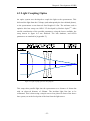
4.3 Light Coupling Optics ....................................................................................... 55
4.4 System Malfunction Evaluation ........................................................................ 56
4.4.1 EPROM: ..................................................................................................... 56
4.4.2 Stepper Motor: ........................................................................................... 56
4.4.3 Mirror: ....................................................................................................... 58
4.4.4 PTG Cable: ................................................................................................ 58
4.4.5 Software: .................................................................................................... 58
4.4.6 PTG Card/Timing: ..................................................................................... 59
4.5 Grating Efficiencies .......................................................................................... 65
4.6 Dummy’s Guides .............................................................................................. 66
5. Development of Pressure Apparatus ................................................................... 69
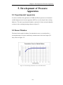
5.1 Experimental Apparatus .................................................................................... 69
5.2 Dome Window .................................................................................................. 69
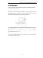
5.3 Sample Stage ..................................................................................................... 71
-i-
5.5 Optical Fibre...................................................................................................... 72
5.4 Vacuum Apparatus ............................................................................................ 74
5.5 General High Pressure/Vacuum Apparatus ...................................................... 75
5.6 Leak Detection and Calibration ........................................................................ 76
5.7 Optical Bench Layout Incorporating Vacuum Chamber .................................. 77
6. Experimental Results ............................................................................................ 78
6.1 Development of Experimentation Techniques .................................................. 78
6.1.1 General Experimental Parameters ............................................................ 78
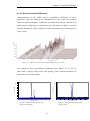
6.1.2 Characterisation/Calibration..................................................................... 79
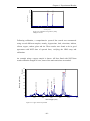
6.1.3 Optimum Fluence ....................................................................................... 81
6.1.4 Imaging ...................................................................................................... 84
6.1.5 Matrix Identification .................................................................................. 85
6.2 Depth Profiling .................................................................................................. 88
6.3 Samples ............................................................................................................. 94
6.3.1 Silicon......................................................................................................... 94
6.3.2 Sandstone ................................................................................................... 95
6.3.3 Slate ............................................................................................................ 96
6.3.4 Marble ........................................................................................................ 97
6.4 Energy-dispersive X-ray spectroscopy (EDX).................................................. 99
6.5 Temporal Delay............................................................................................... 102
6.6 Gate Width Variations..................................................................................... 109
6.7 Power Variations ............................................................................................. 111
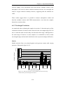
6.8 Surface Weathering ......................................................................................... 116
6.9 Pressure and Gaseous Content Variations....................................................... 125
6.9.1 Pressure Variations.................................................................................. 125
6.9.2 Ambient Gas Interference ........................................................................ 136
6.9.3 Wavelength Variations ............................................................................. 139
7. Errors, Conclusions and Further Work ........................................................... 145
7.1 Errors ............................................................................................................... 145
7.2 Conclusions ..................................................................................................... 147
7.3. Further Work .................................................................................................. 152
References ................................................................................................................ 153
Appendices ............................................................................................................... 161
Appendix A: .......................................................................................................... 161
Comparative study of laser induced breakdown spectroscopy and secondary
ion mass spectrometry applied to dc magnetron sputtered as-grown copper
indium diselenide (CIS) ..................................................................................... 161
Appendix B: .......................................................................................................... 168
LIBS and Remote Raman Spectroscopy References By Los Alamos National
Laboratory (LANL) and Collaborators............................................................. 168
Appendix C: .......................................................................................................... 169
Theoretical Models of the Laser-Solid Interaction49 ........................................ 169
Appendix D: .......................................................................................................... 170
Acton Research Corporation, SpectraPro 500i Specifications: ....................... 170
Appendix E: .......................................................................................................... 172
Grating Efficiency Curves ................................................................................. 172
Appendix F:........................................................................................................... 173
Lens Database, compiled by N. Lucas: ............................................................. 173
Lens Data: ......................................................................................................... 176
Paraxial Constants: .......................................................................................... 176
-ii-
Appendix G: .......................................................................................................... 177
Controller/Software Sweeps, Author N. Lucas ................................................. 177
Appendix H: .......................................................................................................... 185
Dummys Guide to:............................................................................................. 185
Acton Spectrometer with WinSpec and Grams software. ................................. 185
Author N. Lucas ................................................................................................ 185
Appendix I: ........................................................................................................... 196
Dummys Guide to:............................................................................................. 196
Spectrophotometer plotting operation .............................................................. 196
Author N. Lucas ................................................................................................ 196
Appendix J: ........................................................................................................... 197
Dummys Guide to:............................................................................................. 197
Conversion from WinSpec to Grams & Multifile Building ............................... 197
Author N. Lucas ................................................................................................ 197
Appendix K: .......................................................................................................... 200
Notes pertaining to catalogue data of elemental line spectra........................... 200
Appendix L: .......................................................................................................... 203
Pascal program for spectral line search, Author N. Lucas .............................. 203
Appendix M: ......................................................................................................... 207
Access queries to interrogate spectral data, Author N. Lucas.......................... 207
Appendix N: .......................................................................................................... 209
VBA program for spectral line search, Author N. Lucas .................................. 209
Appendix O: .......................................................................................................... 212
VBA programmes for data analysis, correlation and formatting. Author N.
Lucas ................................................................................................................. 212
Appendix P:........................................................................................................... 217
Pascal program to analyse the intensity of selected emission peaks, Author
N. Lucas ............................................................................................................ 217
Appendix Q: .......................................................................................................... 219
Pascal program to calculate the relative standard deviation of a dataset,
Author N. Lucas ................................................................................................ 219
Appendix R: .......................................................................................................... 220
Dummys Guide to:............................................................................................. 220
Acquire a Depth Profile .................................................................................... 220
Author N. Lucas ................................................................................................ 220
-iii-
List of Tables
Table 1.1:
Table 3.1:
Table 3.2:
Table 3.3:
Table 3.4:
Table 4.1:
Table 4.2:
Table 4.3:
Table 6.1:
Table 6.2:
Table 6.3:
Table 6.3:
Pressure and Gaseous environments within the chosen
experimental range1-3.
Doppler and Stark widths from literature34, with electron densities
of 1017.cm-3.
Energy ordering of subshells
Spectroscopic notation with respect to azimuthal quantum
number.
Pressure values and corresponding mean free paths. (calculated
from equation 3.20)
Table showing wavelength reproducibility errors, Grating
2400g/mm
Table showing wavelength reproducibility errors, Grating
600g/mm
Table showing wavelength reproducibility errors, Grating
150g/mm.
Elemental ratios of constituents in sandstone
Elemental ratios of constituents in weathered sandstone
Elemental ratios of constituents in pale slate
Elemental ratios of constituents in dark slate
-iv-
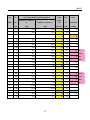
List of Figures
Figure 1.1:
Figure 1.2:
Figure 1.3:
Figure 1.4:
Figure 2.1:
Figure 3.1:
Figure 3.2:
Figure 3.3:
Figure 3.4:
Figure 3.5:
Figure 3.6:
Figure 3.7:
Figure 3.8:
Figure 3.9:
Figure 3.10:
Figure 3.11:
Figure 3.12:
Figure 3.13:
Figure 3.14:
Figure 4.1:
Figure 4.2:
Figure 4.3:
Figure 4.4:
Figure 4.5:
Figure 4.6:
Figure 4.7:
Figure 4.8:
Figure 4.9:
Figure 4.10:
Figure 4.11:
Figure 4.12:
Figure 4.13:
Figure 4.14:
Illustrative study of LIBS timeline. (Composite drawn from many
sources)
Image of the atmospheric regions of Titan in comparison to
Earth5.
Possible present-day structure of Titan’s interior12.
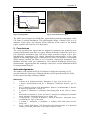
Image of Titan’s surface taken by the Huygens lander on January
14th, 200514.
LIBS publications by year groupings30
Illustration of the pumping arrangement of a Nd:YAG laser.
Surelite laser optical layout
Illustration of possible transitions of electrons. (Composite drawn
from many sources)
Schematic diagram of plasma propagation34
Graph showing matrix effect evident in samples containing both
sand and lead80.
Saha factors applied to nitrogen99 (pressure=0.1Pa)
Energy level diagram for one electron atom. (composite drawn
from many sources)
Influences on atomic energy levels103.
Absorption bands of methane from 750-940nm114
Image of total internal reflection inside a optical fibre.
Illustration of diffraction parameters for a grating.
Illustration of diffraction parameters for a blazed grating.
An image intensifier tube
Illustration of timing requirements for LIBS experiments.
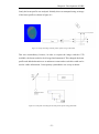
Setup and image of beam profile capture using CCD camera
Setup and circuit diagram of beam profile capture using
photodiode
Charts showing beam profile from photodiode capture, the
different colours represent the beam intensity
Light coupling optics lens setup diagram
Transmission response of orange perspex.
Schematic of the system timing using pulse generator
Circuit diagram of impedance matching circuit
Circuit diagram of delay circuit
Schematic of the system timing using delay and impedance
circuit.
Schematic of the system timing, showing redundant parts of
system to be removed for calibration.
Schematic of the system timing, showing setup with external
timing box.
Schematic of the final arrangement for the timing setup of the
LIBS system
Schematic of the final arrangement for the timing setup of the
LIBS system, with inherent delays shown.
Intensity versus wavelength chart for mercury lamp emissions
obtained from spectrometer captures and NIST values.
-v-
Figure 4.15:
Figure 4.16:
Figure 5.1
Figure 5.2:
Figure 5.3:
Figure 5.4:
Figure 5.5:
Figure 5.6:
Figure 5.7:
Figure 5.8:
Figure 5.9:
Figure 5.10:
Figure 5.11:
Figure 5.12:
Figure 5.13:
Figure 5.14:
Figure 5.15:
Figure 5.16:
Figure 5.17:
Figure 6.1:
Figure 6.2:
Figure 6.3:
Figure 6.4:
Figure 6.5:
Figure 6.6:
Figure 6.7:
Figure 6.8:
Figure 6.9:
Figure 6.10:
Figure 6.11:
Figure 6.12:
Figure 6.13:
Figure6.14:
Figure 6.15:
Figure 6.16:
Figure 6.17:
Figure 6.18:
Grating efficiencies versus wavelength
Intensity versus wavelength for gratings corrected for their
efficiency wavelength response
Working drawings of HPVA chamber
Chart showing transmission curve for the HPVA dome.
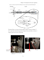
Image to show micrometer feedthroughs of sample stage on the
HPVA
Image to show sample stage and coupling bracket
Image of configuration of fibre bundle at the spectrometer end
Drawing of optical fibre feedthrough, courtesy of John Cowpe and
Richard Pilkington
Image showing alignment of fibre end
Image showing optical fibre feedthrough
Schematic of vacuum apparatus setup
Schematic of high pressure/vacuum apparatus setup
Calibration of 100sccm MFC
Calibration of 20sccm MFC
Rate of fill of HPVA
Leak rate of vacuum apparatus
Image of Praxair Bourdon gauge
Average of three sets of measurements for calibration of the
Bourdon gauge when used at pressures below atmospheric
Schematic of optical bench setup
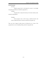
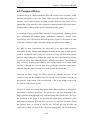
Graph showing fluctuations in cadmium lamp intensity over time
Calibration using mercury lamp, 150grooves/mm grating
Calibration using mercury lamp, 600grooves/mm
Calibration using mercury lamp, 2400grooves/mm
Copper emission spectrum
Chart showing fluence at varying distances from the focal point of
the final lens
Emission intensity versus distance from focal point for CIS and its
constituents
Spectrometer image of cadmium emission lines
Imaged size of spectrometer entrance slit versus actual vernier
reading
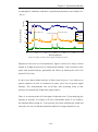
Spectral responses of solder matrix and its constituent parts
Solder emission spectrum
Addition of constituent species emission spectra. (Sn, Pb, Cu,
rosin flux)
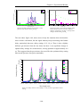
Solder emission spectrum minus lead emission spectrum
Solder emission spectra minus lead and tin emission spectra
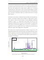
Solder emission spectrum minus lead, tin and copper emission
spectra
Solder emission spectrum minus lead, tin and copper emission
spectra
Shot versus intensity plot to illustrate removal of CIS on silicon
substrate, 1.33x10⁸Wcm-2
Shot versus intensity plot to illustrate removal of CIS on glass
substrate, 1.33x10⁸Wcm-2
-vi-
Figure 6.19:
Figure 6.20:
Figure 6.21:
Figure 6.22:
Figure 6.23:
Figure 6.24:
Figure 6.25:
Figure 6.26:
Figure 6.27:
Figure 6.28:
Figure 6.29:
Figure 6.30:
Figure 6.31:
Figure 6.32:
Figure 6.33:
Figure 6.34:
Figure 6.35:
Figure 6.36:
Figure 6.37:
Figure 6.38:
Figure 6.39:
Figure 6.40:
Figure 6.41:
Figure 6.42:
Figure 6.43:
Figure 6.44:
Figure 6.45:
Figure 6.46:
Figure 6.47:
SIMS comparison of copper, indium and selenium depth
distributions
RBS plot showing experimental results cross referenced with
simulated results
Images of ablation crater’s on thin film CIS sample deposited on
silicon.
SEM image showing an ablation crater
Image of silicon sample after laser ablation, the circles are
ablation craters.
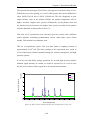
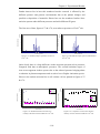
Silicon sample in atmospheric conditions, 150g/mm grating
Silicon Sample in atmospheric conditions, 2400g/mm grating
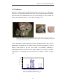
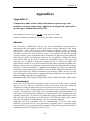
Images of sandstone samples, with ablation craters clearly visible.
Both were taken from a larger block shown on the left, where
organic residues can be seen building up on the surface, the clean
stone visible underneath.
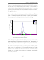
Sandstone sample emission spectrum in atmospheric conditions,
2400g/mm
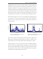
Slate sample showing ablation craters and re-deposition of
material around the crater.
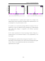
Pale slate sample in atmospheric conditions, 2400g/mm grating
Dark slate sample in atmospheric conditions, 2400g/mm grating
Pale slate sample in 1 bar nitrogen fill, 2400g/mm grating
Dark slate sample in 1 bar nitrogen fill, 2400g/mm grating
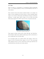
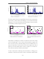
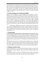
Images of marble samples, the one on the left showing the
crystalline structure, the one on the right showing the ablation
craters and in some cases the re-deposition from a partial or full
methane content atmosphere.
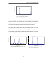
Marble sample in atmospheric conditions, 2400g/mm grating
Marble sample emission spectrum, 1 bar nitrogen fill, 2400g/mm
grating
Marble sample emission spectrum, in vacuum as emission lines
exhibit self-reversal at other pressures, 2400g/mm grating
Sandstone EDX image
Sandstone EDX image, 4* original magnification to resolve iron
and copper peaks.
Weathered sandstone EDX image
EDX Image of marble sample
Pale slate EDX image
Dark slate EDX image
Delay variation, silicon sample, atmospheric pressure
Delay variation, silicon sample, 1.5 bar pressure of gas mixture
94%N2 6%CH4
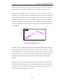
Delay versus emission intensity of the silicon emission line at
251.61 nm in different samples. Averaged over 15 shots, 1.5 bar
pressure with gas mixture 94%N2 6%CH4
Delay variation, silicon sample, 1.5 bar pressure of gas mixture
93%N2 7%CH4.
Delay variation, silicon sample, under vacuum pressure of 3x10⁻⁴
mb.
-vii-
Figure 6.48:
Figure 6.49:
Figure 6.50:
Figure 6.51:
Figure 6.52:
Figure 6.53:
Figure 6.54:
Figure 6.55:
Figure 6.56:
Figure 6.57:
Figure 6.58:
Figure 6.59:
Figure 6.60:
Figure 6.61:
Figure 6.62:
Figure 6.63:
Figure 6.64:
Figure 6.65:
Figure 6.66:
Figure 6.67:
Figure 6.68:
Figure 6.69:
Figure 6.70:
Figure 6.71:
Figure 6.72:
Figure 6.73:
Figure 6.74:
Figure 6.75:
Figure 6.76:
Figure 6.77:
Delay variation, sandstone sample, under vacuum pressure of
5x10⁻² mb.
Silicon pressure variations, delay 600 ns
Silicon delay variations, pressure 3x10⁻⁴mb
Silicon delay variations, pressure 4x10⁻⁶mb
Width variation in microseconds at 1.5 bar with 6% CH4 94% N2
gaseous mixture, silicon sample
Width variation in microseconds at 1.5 bar with 6% CH4 94% N2
gaseous mixture, silicon sample
Width variation in microseconds at 1.5 bar with 5% CH4 95% N2
gaseous mixture, silicon sample
Width variation in microseconds at 1.5 bar with 7% CH4 93% N2
gaseous mixture, silicon sample
Width variation in microseconds at 1.5 bar with 6% CH4 94% N2
gaseous mixture, sandstone sample
Schematic diagram of optical bench setup for power variations
Power output with relation to iris size
Power variation (mJ/pulse) on silicon sample, gas composition:
5%CH4 95%N2
Power variation (mJ/pulse) on sandstone sample, gas composition:
5%CH4 95%N2
Power variation (mJ/pulse) on silicon sample, gas composition:
7%CH4 93%N2
Power Variation on Sandstone Sample, gas composition: 6%CH4
94%N2
Averaged over 15shots, Power Variation on Sandstone Sample,
gas composition: 6%CH4 94%N2
Logarithmic plot of power variation, sandstone sample, gas
composition: 6%CH4 94%N2
Power variation on silicon sample, gas composition: 6%CH4
94%N2
Power variation on weathered sandstone sample, gas composition:
6%CH4 94%N2
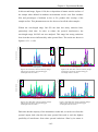
Weathered sample 3D emission spectra, 15 shots
Weathered sample spectrum, first shot
Weathered sample spectrum, fifteenth shot
Image of weathered sandstone sample, showing green algae buildup.
Weathered surface emission intensity reduction with shot number
in atmospheric conditions
Comparison of silicon line emission intensity increase with shot
number in atmospheric conditions
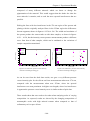
Weathered sample spectrum, first shot at 5x10⁻² mb
Weathered sample spectrum, fifteenth shot at 5x10⁻² mb
Weathered surface lines emission intensity reduction with shot
number at 5x10⁻² mb
Comparison of silicon line emission intensity increase with shot
number at 5x10⁻² mb
Weathered sample emission spectrum, first shot at 1.5 bar
nitrogen fill
-viii-
Figure 6.78:
Weathered sample emission spectrum, fifteenth shot at 1.5 bar
nitrogen fill
Figure 6.79: Weathered surface lines emission intensity reduction with 1.5 bar
nitrogen fill
Figure 6.80: Comparison of silicon line emission intensity increase with shot
number at 1.5 bar nitrogen fill
Figure 6.81: Weathered sample emission spectrum, first shot at 1.5 bar
methane fill
Figure 6.82: Weathered sample emission spectrum, fifteenth shot at 1.5 bar
methane fill
Figure 6.83: Weathered surface lines emission intensity reduction with a 1.5
bar methane fill
Figure 6.84: Comparison of silicon line emission intensity increase with shot
number with a 1.5 bar methane fill
Figure 6.85: Silicon and iron emission line intensity increase with shot number
Figure 6.86: Weathered sample emission spectrum, first shot at 1.5 bar,
6%CH4 94%N2 fill
Figure 6.87: Weathered sample emission spectrum, fifteenth shot at 1.5 bar,
6%CH4 94%N2 fill
Figure 6.88: Weathered surface lines emission intensity reduction with shot
number, 1.5 bar 6%CH4 94%N2 fill
Figure 6.89: Comparison of silicon line emission intensity increase with shot
number, 1.5 bar 6%CH4 94%N2 fill
Figure 6.90: Single shot emission spectrum of silicon sample showing intensity
change with pressure, with N2 as filling gas
Figure 6.91: 15 shot average, silicon sample, intensity change with pressure,
with N2 as filling gas
Figure 6.92: Silicon sample emission intensity change with pressure, with
5%/95% mixture as filling gas, variation in millibar
Figure 6.93: Silicon sample emission intensity change with pressure, with
6%94% mix as filling gas, variation in millibar
Figure 6.94: Simplified silicon sample emission intensity change with pressure,
with 6%94% mix as filling gas, variation in millibar
Figure 6.95: Silicon sample emission intensity change with pressure, with
7%/93% mixture as filling gas, variation in millibar
Figure 6.96: Silicon sample emission intensity change with pressure, with CH4
as filling gas, variation in millibar
Figure 6.97: Sandstone sample emission intensity change with pressure, with
N2 as filling gas, variation in millibar
Figure 6.98: Sandstone sample emission intensity change with pressure, with
CH4 as filling gas, variation in millibar
Figure 6.99: Sandstone sample emission intensity change with pressure, with
6%/94% mix as filling gas, variation in millibar
Figure 6.100: Simplified sandstone samples emission intensity change with
pressure, with 6%94% mix as filling gas, variation in millibar
Figure 6.101: Chart showing emission intensity change with pressure, with N2
as filling gas, silicon sample.
Figure 6.102: Change in emission intensity with pressure variations, 5/95 mix as
filling gas, silicon sample
-ix-
Figure 6.103: Change in emission intensity with pressure variations , 6/94 mix
as filling gas, silicon sample
Figure 6.104: Change emission intensity with pressure variations, 7/93 mix as
filling gas, silicon sample
Figure 6.105: Change emission intensity with pressure variations, CH4 as filling
gas, silicon sample.
Figure 6.106: Plot of specific emission line intensity variations from each
sample with respect to pressure.
Figure 6.107: Silicon sample, emission signal with different gaseous content at
1.5 bar
Figure 6.108: Silicon sample, carbon line emission signal with different gaseous
content at 1.5 bar
Figure 6.109: Silicon sample, carbon emission intensity for various gas fills
Figure 6.110: Silicon sample, carbon and silicon emission intensities for various
gas fills
Figure 6.111: Plot of silicon and carbon emission intensities from silicon
sample, normalised to silicon.
Figure 6.112: Sandstone sample, carbon and silicon emission intensities for
various gas fills
Figure 6.113: Plot of silicon and carbon emission intensities from sandstone
sample, normalised to silicon
Figure 6.114: Marble sample, carbon, silicon and oxygen emission intensities
for various gas fills
Figure 6.114: Plot of silicon, carbon and oxygen emission intensities from
marble sample, normalised to silicon
Figure 6.115: Emission intensities of various marble emission lines showing
variations due to pressure and gaseous content
Figure 6.116: Pressure variation of Ca(II) 393.37nm and Ca (II) 396.85nm in
marble, with N2 fill. Showing self reversal due to pressure.
Figure 6.117: Simplified Pressure variation of Ca(II) 393.37nm and Ca (II)
396.85nm in marble, with N2 fill. Showing self reversal due to
pressure.
Figure 6.118: Pressure versus intensity variation of calcium emission lines from
marble sample, with nitrogen filling gas.
Figure 6.119: Image of dark slate sample showing ferrous reduction spheres.
Figure 6.120: Image of slate sample showing ‘sooting’ of the surface from redeposition at the ablation craters.
Figure 6.121: Pale slate, emission intensity change with pressure variations,
nitrogen filling gas, wavelength centre at 252nm.
Figure 6.122: Pale slate, emission intensity change with pressure variations,
nitrogen filling gas, wavelength centre at 276nm.
Figure 6.123: Dark slate, emission intensity change with pressure variations,
nitrogen filling gas, wavelength centre at 252nm.
Figure 6.124: Dark slate, emission intensity change with pressure variations,
nitrogen filling gas, wavelength centre at 276nm.
Figure 6.125: Pale slate, pressure versus intensity variations with nitrogen filling
gas
Figure 6.126: Dark slate, pressure versus intensity variations with nitrogen
filling gas
-x-
Figure 7.1:
Figure 7.2:
Figure 7.3:
Figure 7.4:
Figure 7.5:
One standard deviation of delay versus emission intensity of the
silicon emission line at 251.61 nm in different samples. Averaged
over 15 shots, 1.5 bar pressure with gas mixture 94%N2 6%CH4
One standard deviation of power versus intensity variations on
sandstone sample, gas composition: 6%CH4 94%N2
One standard deviation of change in intensity with pressure, with
N2 as filling gas, silicon sample.
One standard deviations of change in intensity with pressure, with
6/94 mix as filling gas, silicon sample
One standard deviation of change in intensity with pressure, with
CH4 as filling gas, silicon sample.
-xi-
Acknowledgements
I would initially like to thank all those I worked closely with in the Laser Group
at Salford University. To Richard Pilkington for his help and his enthusiasm with
P.L.O.P. and Christmas escapes to the country. Robin Hill, without his help to
pull it out of the bag I would never have submitted my thesis. Stuart Astin for his
kindness of heart and quiet unassuming knowledge and patience with lessons.
Helen Brown for mutual expulsion of stress and ‘ciggie break’ escapes. To John
Cowpe for his knowledge on vacuum apparatus and systems and to Garry
Rowsell for his ‘think tank’ help.
Thanks must go to other staff at Salford University. Jay Smith, for his ingenuity.
Steve Hurst and Mike Hulme for their workshop ‘wizardary’. To Bruce (and the
voices) and Paul Murphy for their PC know how. Graham Keeler and Brian
James for their computer programming and interfacing help. Allan Boardman for
his valuable support. Dave armour for his guidance on plasma processes and
Keren Maloney for her help and patience with administration support.
External to the university I would like to thank Nigel Murphy and John
Wilkinson at Universal Imaging Corporation for their continued support
throughout the project.
I give thanks to EPSRC for my funding. I also would like to thank the institutions
who made it possible for me to attend conferences with their generous financial
support, namely; The Rank Prize Funds; The European Space Agency, The
International Astronautics Federation and to Dave Wright of the British Rocketry
Oral History Programme.
Thank you to my friends, who I am very lucky to say are too numerous to name,
for their help in all things, especially the low times. I give special thanks to Liz
Forshaw for unwavering support in all things non-physicsy. To Chris Rollins and
Adam Theis for their invaluable CAD help. To my Physiotherapist Byron
Clithero, without his help I would still be in agony, unable to work.
-xii-
Not least I give thanks to my family, without their help, support and love I would
have never achieved such dizzy heights!
Declaration
The computer programs and dummy’s guides written in this work have been
developed by the thesis author.
-xiii-
Abbreviations
ADC
CCD
CF-LIBS
CIS
EDX
EPROM
ESA
FO
HPVA
IBM
ICCD
KTP
LANL
LASER
LED
LIBS
LOD
LSAW
LSCW
LSDW
LSRW
LTE
LTSD
MCP
MFC
MFP
MUT
NASA
Nd:YAG
NIST
PCB
PTG
RBS
SEM
SIMS
TEM00
UV-VIS
VBA
Astronomical Data Centre
charged-coupled device
calibration free laser induced breakdown spectroscopy
copper indium diselenide
X-Ray dispersive analysis
electronic prompt
European Space Agency
optical fibre
high pressure/vacuum apparatus
International Business Machines Corporation
intensified charged-coupled device
potassium titanyl phosphate
Los Alamos national laboratory
light amplification by stimulated emission of radiation
light emitting diode
laser induced breakdown spectroscopy
limit of detection
laser-supported absorption wave
laser-supported combustion wave
laser-supported detonation wave
laser-supported radiation wave
local thermodynamic equilibrium
lens to surface/sample distance
micro-channel plate
mass flow controller
mean free path
material under test
National Aeronautics Space Administration
neodymium: yttrium-aluminum-garnet
National Institute of Standards and Technology
printed circuit board
programmable timing generator
Rutherford Backscattering
scanning electron microscope
secondary ion mass spectrometry
fundamental transverse mode
ultraviolet-visible
visual basic for applications
-xiv-
Abstract
Laser induced breakdown spectroscopy (LIBS) is a technique that can determine
the elemental composition and quantities of a sample by the spectral analysis of a
laser induced plume.
This study was undertaken to develop, characterise and assess the use of the
LIBS technique on geological samples in different pressure and gaseous
environments. The experimental range chosen was dictated by the planetary
conditions on Titan and other extra-terrestrial bodies with the samples analysed
chosen to complement a range of rock types.
A LIBS system was developed, together with associated experimental apparatus
able to acquire results in varying pressure and gaseous environments. The
capability of LIBS to analyse weathered rock samples was investigated under
various ambient conditions; pressures of 160x103 Pa to 0.4x10⁻³ Pa and ambient
gaseous mixtures of air, nitrogen and methane.
Particular attention was paid to temporal and power considerations under such
regimes. As was expected, the chosen delay time to optimise the emission signals
needed to be increased with increasing ambient pressure. At power values as low
as 28.5 mJ/pulse (using a 6 ns pulse from a doubled Nd:YAG laser at 532 nm) a
valid emission signal could be obtained. Increasing the laser power resulted in a
reduction in the overall signal to noise ratio.
It was observed that ambient methane quenches the optical emission signal due
to non-radiative transitions. In spite of this, valid qualitative data are obtainable,
even when emissions due to carbon transitions from both the sample and the
gaseous environment, are present.
Results are presented which support the premise that the LIBS technique can be
used to investigate both the surface and depth compositions of geological
samples under extra-terrestrial conditions.
-xv-
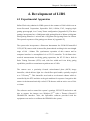
Chapter 1: Introduction
1. Introduction
1.1 Background
The main thrust of this research study was to fully commission a laser induced
breakdown spectroscopy (LIBS) system for use at Salford University. This
equipment was developed to incorporate apparatus able to analyse LIBS in
varying pressure environments.
Once commissioned a study was undertaken to examine the effects of pressure
and different gaseous environments on the LIBS technique, paying particular
attention to temporal affects and power considerations. The environments chosen
varied from pressures of 160x103 Pa to 0.4x10⁻³ Pa with different gaseous
mixtures of air, nitrogen and methane.
This work was personally carried out from conception to completion, with a view
to ascertaining the ability of the LIBS technique to acquire good analytical data
in the atmosphere of the moon Titan, a previously unexplored experimental
environment.
LIBS is a technique that can determine the elemental composition and quantities
of a sample by analysis of emission from a laser induced plume. A high power
laser is focused onto the material of interest creating a plume; this plume expands
over time and spectral emissions result from the relaxation of the constituent
excited species. The atomic spectral lines are then used to analyse the material.
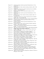
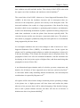
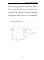
The timeline involved in LIBS analysis can be broken down and summarised,
illustrated in figure 1.1, each section being explained in greater detail in the
following theory chapter.
1) Incidence of the laser pulse upon the sample.
2) Absorption and heating of the sample via the incident laser energy
3) Priming electrons initiate the laser ablation process
4) The surface of the sample is broken down and ablated.
-1-
Chapter 1: Introduction
5) The plume itself acts to shield the sample surface from the remaining
incident laser light.
6) After the laser pulse finishes the plume expands away from the surface
7) Once the plume has dissipated some constituents may be re-deposited on
the sample surface.
Figure 1.1: Illustrative study of LIBS timeline.
(Composite drawn from many sources)
-2-
Chapter 1: Introduction
1.2 Planet and Moon Environments
The experimental range chosen accounted for the atmospheric conditions on
varying moons and planets in our solar system, paying particular attention to that
of Titan, one of the moons of Saturn.
LIBS is of particular interest for space applications due to its capability for use at
stand-off distances, thus eliminating the possibility of cross contamination of
samples. Titan is one of the moons of Saturn and of particular importance as it is
the only known moon with a fully developed thick atmosphere that is rich in
organic compounds. As such Titan may be a clue as to how life began on Earth.
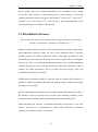
Planets and moons that lie within the experimental parameters used in this study
are shown in table 1.1. As can be seen, many atmospheric pressures fall within
the experimental range, as do some gaseous atmospheric contents. As such the
results obtained in this study could prove valuable for many extra-terrestrial
applications.
Table 1.1: Pressure and Gaseous environments within the chosen experimental range1-3.
Planet
Moon
Atmospheric
Gaseous atmospheric content
pressure
(millibar)
Titan
1500
98.4% nitrogen and 1.6% methane
Triton 0.01
99.9% nitrogen, 0.1% methane
carbon dioxide 95.32%, nitrogen 2.7%, argon
Mars
7.6
1.6%, oxygen 0.13%
hydrogen 83%, helium 15%, methane 1.99%,
Uranus
1200
ammonia 0.01% plus traces of other gases
hydrogen 84%, helium 12%, methane 2%,
Neptune
1000-3000
ammonia 0.01%, plus traces of other gases
trace amounts of methane, water vapour and
Jupiter
700
ammonia
Saturn
1400
molecular hydrogen
Pluto
0.0015-0.003 nitrogen & methane
Europa 1.00E-08
methane 10.5 ppb
Table 1.1: Pressure and gaseous environments within the chosen experimental range1-3.
-3-
Chapter 1: Introduction
Previous studies have been undertaken to ascertain the capability of the LIBS
technique in Martian, Venetian and the low pressure environments of moons and
asteroids. These are described in sections 2.3 and 3.7.
These reports have been so successful that missions have been plannedI1
incorporating a LIBS instrument for analysis of rocks and soils on the Martian
surface. The first mission is being planned for launch in 2009, on board the
NASA’s Mars Science Laboratory and the second, a LIBS-Raman combined
instrument, is being planned to launch in 2011 by the European Space Agency on
the ExoMars rover mission.
To complement these studies this research was aimed at Titan, to establish if this
technique can also be used in this distinct and currently un-explored
environment.
Since this study was undertaken, new data has been acquired from a mission to
Saturn and Titan. The spacecraft in this mission is called Cassini-Huygens, and it
reached Saturn on July 1, 2004, the first Huygens data being reported by ESA on
January 21st 2005.
Previously Titan had been examined by the space missions Voyager 1 and
Voyager 2. Voyager 1’s mission had been diverted specifically to make a closer
pass of Titan, but unfortunately this mission’s instrumentation range did not
include an instrument that could penetrate Titan’s haze.
Since the Cassini-Huygens probe much more information is known or has been
validated about the atmosphere, surface and composition of Titan. At Titan’s
surface the temperature mean is 94K, (-179oC). This low temperature is
significant as at these temperatures water ice does not sublimate, and as such the
atmosphere is nearly free of any water vapour4. Titans atmospheric pressures
were thought to be 1.5 bar (150 kPa), and have since been confirmed to be 1.467
bar, (146.7 kPa).
-4-
Chapter 1: Introduction
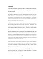
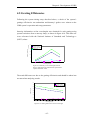
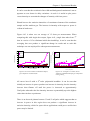
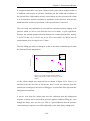
Figure 1.2: Image of the atmospheric regions of Titan in comparison to Earth5.
Figure 1.2: Image of the atmospheric regions of Titan in comparison to Earth5.
Titan’s atmosphere is now known to contain 98.4% nitrogen and 1.6% methane,
but this methane content is known to increase to 5% near the surface and there
has been indication that the surface landing site of the Huygens probe was
soaked in methane6.
The amount of methane abundant in Titan’s atmosphere is somewhat a mystery
as the solar winds in the early solar system should have cleared the atmosphere
of methane content. Leading theories believe that in early formation, methane
was frozen as water-ice or ‘clathrates’ which have since melted releasing
methane into the atmosphere.
At the time of implementation of experimentation, (before the Cassini-Huygens
mission data was obtained on atmospheric composition), the compositional
content of Titan was thought to be 94% nitrogen and 6% methane. A percent
variance of these compositions was covered in the experimental parameters.
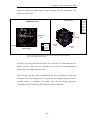
-5-
Chapter 1: Introduction
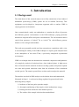
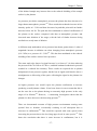
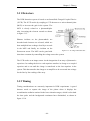
1.3 Rock Composition
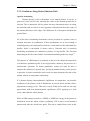
At the time of experimentation, the types of rock found
on Titan were virtually unknown. It was thought that
there were seas of liquid hydrocarbons7 and that Titan’s
bulk composition was water ice with approximately 65%
rock-metal material8. It was proposed that Titan was
dense due to its gravitational compression9 and its
structure was differentiated into several layers composed
of different crystal forms of ice10 and that its interior may
once have contained a hot liquid layer consisting of water
and ammonia between the ice crust and the rocky core11.
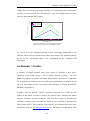
Figure 1.3: Possible present-day structure of Titan’s interior12.
Figure 1.3: Possible present-day
structure of Titan’s interior12.
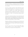
Taking into account these suppositions, rock
types
were
chosen
with
a
range
of
composition elements of metamorphic rock
types. Slate was chosen as a foliated
metamorphic rock type. Marble was also
chosen as a metamorphic calcite rock.
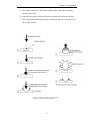
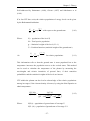
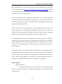
Subsequent to choosing the above rock types
further information was obtained via radar
from
the
information
Cassini
conflicted
spacecraft13.
with
This
information
previous thoughts that there were seas of
hydrocarbons at the equator. Radar images
revealed that these regions were in fact
extensive plains covered in longitudinal sand
dunes. As a result of this information
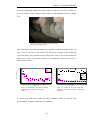
Figure 1.4: Image of Titan’s surface
taken by the Huygens lander on January
14th, 200514.
sedimentary sandstone was also chosen for
testing.
Figure 1.4: Image of Titan’s surface taken by the Huygens
lander on January 14th, 200514.
-6-
Chapter 1: Introduction
The rock types chosen had varying compositions, not only across the samples but
inherently within the samples themselves. The samples are inevitably complex
with non-uniformity in their composition, particularly so in the case of the slate
sample. The thrust of this work is the feasibility of the LIBS analytical technique
to analyse these samples in these environments. Consequently, account must be
taken of the ambiguous composition of the rock types.
-7-
Chapter 2: History and Uses
2. History and Uses
2.1 Scientific History of LIBS
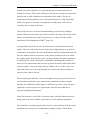
LIBS was first published in the report by Brech and Cross in 1962, which
observed emission spectra from a metal target using a ruby maser15. In 1963 the
paper published by Debras-Guédon and Liodec16 described first analytical use of
LIBS using a ruby laser to produce excited spectral emissions of the elements. In
1964 the first use of a Nd:YAG laser was reported by Geusic17 et al from Bell
Labs. In the same year Maker, Terhune and Savage18 reported the first
observation of optically-induced breakdown in a gas.
In the early 1970’s Moenke-Blankenburg19 wrote a review on LIBS with crossexcitation, and in the late 1980’s the same author produced the book ‘Laser
Microanalysis20’, which also provided another comprehensive review of the
analytical applications of laser-target interactions.
The first people to use LIBS to determine the chemical composition of a
substance were L. Radziemski and D. Cremers in the 1980’s. In this century
many papers were produced by this duo with collaboration from colleagues,
some such papers are stated in the references21-28. These papers varied from timeresolved techniques to chemical detection of gases, liquids, aerosols and solids.
This work culminated in the book, Laser-Induced Plasmas and Applications
written by L.J. Radziemski and D.A. Cremers in 198929.
-8-
Chapter 2: History and Uses
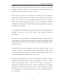
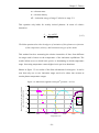
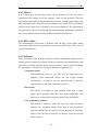
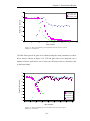
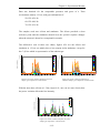
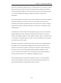
In the 1980’s only a handful of groups were working on LIBS; this number has
increased exceedingly since then, as shown in figure 2.1.
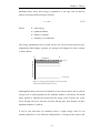
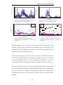
Figure 2.1: LIBS Publications by year groupings30
250
Number of Publications
203
200
150
100
50
36
8
15
0
81-85
86-90
91-95
96-2000
Years
Figure 2.1: LIBS publications by year groupings30
In the late 1990’s, with the advent of high resolution spectrometers, the LIBS
technique really took off. These detectors allowed multiple elements to be
detected at once, with increased sensitivity compared to that of previous
methods.
The first international conference on LIBS was held in 2000 in Pisa, Italy. Since
this date conferences have been held yearly, each alternate year being an
international meeting.
A comprehensive LIBS review paper was written by D. Cremers31 and L
Radziemski in 1987, and another was written in 2002 by L. Radziemski32, which
provides a sense of the technique’s development from inception to the year 2000.
Another thorough review focusing on the effects of experimental parameters on
LIBS analytical performance was provided by E. Tognoni33 et al, early in 2002.
This paper refers to literature of experimental studies from 1988 to 2001.
Lastly, a useful source for the all-inclusive history of LIBS is the Handbook of
Laser Induced Breakdown Spectroscopy34, which provides a broad review from
1960 – 2002.
-9-
Chapter 2: History and Uses
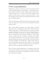
2.3 Uses, Types and Divisions
LIBS analysis is extremely versatile and can be used in many different fields of
research. The LIBS technique offers: rapid analysis - one measurement per laser
pulse; sampling of solids, gases or liquids; simultaneous multi-element detection;
a spatial resolving power of ~1-500 µm; remote analysis capabilities; depthprofiling of layered structures and surface coatings; detection limits of 1-100
ppm, depending on sample composition and instrumental characteristics; all with
little or no sample preparation.
Some of the disadvantages of LIBS range from poor shot-to-shot stability; matrix
effects; poor signal to noise ratio; loss of weaker lines and difficulty in obtaining
quantative analysis.
There are many different applications of the LIBS technique in numerous
different fields. These wide ranging applications include: archaeological analysis
of Minoan dagger history35, elemental composition of artworks to characterise
pigments in a Byzantine work layer by layer36, analysis of bobsleigh runners in
the 2002 winter Olympics to ensure they meet with the Olympic standards in
having a homogeneous metallic composition throughout37, various different
varieties of coating analysis such as Lademann’s investigation into the stability
of coated titanium microparticles used in sunscreens38, dentistry applications,
utilizing the high spatial resolutions possible with LIBS, to identify the transition
from carious (unhealthy) tissue to healthy tissue39, and in the nuclear industry for
remote chemical analysis, exploiting the ability of LIBS to work in submerged
remote environments40,41. These several uses mentioned are just a small selection
that have so far been explored using the LIBS analysis technique.
Most of the above mentioned applications are at atmospheric pressure with
terrestrial gaseous environments. Some research has been undertaken in different
pressure regimes and environments, such applications are useful to ascertain the
uses of LIBS in space exploration.
-10-
Chapter 2: History and Uses
A cross section of papers written by Los Alamos national laboratory (LANL) on
LIBS publications for planetary science are stated in Appendix [B] some
reference summaries are stated here:
LIBS Operation on Airless Bodies4,42, a study undertaken to characterise
the changes to the LIBS plasma spark in different pressure regimes.
LIBS Operation on Venus4,43, these studies concentrate on the hostile
environment of Venus with atmospheric pressures ~90Bars.
Investigation of LIBS feasibility for in situ planetary exploration: An
analysis on Martian rock analogues44
This latter study focuses on volcanic rock analysis in an environment similar to a
Martian one, using the calibration free LIBS (CF-LIBS) method at wavelengths
of 355 nm. It suggests that the technique can be used to allow elemental
qualitative and quantative identification on the silicate minerals studied in the
Martian environment. The CF-LIBS technique was shown to be accurate within
the range 1-30% for the major constituents, but this depended heavily on the
element and its concentration. The accuracy would be reasonable for first line
identification but could be questionable when used in precise analytical
measurements.
LIBS application for analyses of Martian crust analogues: Search for the
optimal experimental parameters in air and CO2 atmosphere45.
This study compares a Terrestrial environment to a Martian environment, with
particular attention paid to the optimal experimental parameters such as emission
intensity, temperature and electron density. It found that the acquisition window
where local thermodynamic equilibrium (LTE) holds is much shorter in Martian
environments due to low electron density and fast plasma cooling and decay, the
latter giving a short interval for maximizing signal to noise ratios.
Further analysis of studies relevant to the work in this thesis are described in the
theory, section’s 3.5, 3.6 & 3.7.
-11-
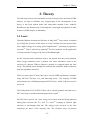
Chapter 3: Theory
3. Theory
The following section will concentrate on each of the processes involved in LIBS
analysis. In order to facilitate easy categorisation of the development of the
theory, it has been broken down into subsections entitled; Laser; Induced;
Breakdown; and Spectroscopy. Following this a thorough investigation of other
features in LIBS analysis is undertaken.
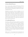
3.1 Laser
Theodore Maiman invented the first laser in May 196046. Laser action is initiated
by exciting the electrons of the atoms in a laser medium from the ground state
into a higher energy level using optical amplification47, producing a population
inversion46. This is achieved by pumping48 the laser medium via the application
of a large amount of energy in the form of broadband light.
As the electrons make transitions back to the ground state they emit radiation.
Most energy transitions emit a phonon, but some transitions result in the
emission of a photon. When a photon is emitted it is trapped within the laser
cavity. This photon passes through the medium and stimulates further emissions
from the population inversion.
There are many types of lasers that can be used in LIBS experiments, examples
being Nd:YAG, Excimer, CO2 and Microchip lasers. The majority of LIBS
measurements use a flashlamp pumped Nd:YAG laser, which is the laser used in
this work.
The Neodymium-YAG (Nd:YAG) laser rod is a doped insulator laser that uses a
Nd3+ion to dope a yttrium-aluminum-garnet host crystal47.
Nd:YAG lasers operate via a four energy level system with the lasing transition
taking place between the 4F3/2 and 4I11/2 states48 resulting in infrared light
emission of wavelength 1064 nm. The energy levels involved in the laser
transitions are those of the impurity ions. The electrons relax via phonon
- 12 -
Chapter 3: Theory
interactions from the third level into the second level of this system which is
known as a metastable state, meaning that it can return to a less excited state only
via a highly inhibited transition. As such, electrons remains in this state for an
appreciable fraction of a second rather than for the lifetime of a typical transition
rate of ~10-8s. It is this long lifetime that provides the mechanism by which a
population inversion can be achieved.
The Nd:YAG laser is a popular choice for laser ablation experiments as it
displays a high spatial coherence and has high output energies49.
Converting the 1064 nm laser output to shorter wavelengths is achieved by
passing the laser beam through a non-linear crystal. This produces harmonics
obtained from phase matching48. The conversion efficiency is approximately
50% and reduces with each harmonic. The crystal used to produce green light of
wavelength 532nm, used in this work, is KTP (potassium titanyl phosphate).
The light emitted by a laser will have different optical frequencies associated
with different modes of the optical resonator. These resonator modes are known
as longitudinal and transverse modes. The longitudinal modes of a laser govern
the spectral characteristics, such as line width and coherence length. The
transverse modes govern the beam divergence, beam diameter and energy
distribution.
A laser that operates in its fundamental transverse mode, or TEM00 mode, emits
light with a Gaussian intensity profile. This light will propagate as a directional
parallel beam for a distance given by πd2/λ, the Rayleigh range, (where d is the
laser output coupler diameter). Beyond this range the beam will expand with a
divergence of ∆θ = d/λ, known as the beam divergence.
- 13 -
Chapter 3: Theory
3.2 Induced (Laser Ablation)
R. Srinivasan and V. Mayne-Banton of IBM Research first reported the laser
ablation phenomenon to produce thin films in 198250. Laser ablation is a process
whereby the short, intense burst of energy delivered by a laser pulse is used to
vaporise a material that would often be impossible to vaporise by conventional
methods51,52. Lasers are advantageous in many ways. Because of their high
spatial coherence they may be focused onto a very small area and this can result
in intense local heating without neighbouring areas being affected. The majority
of the laser energy is deposited near the surface of the target, allowing surface
regions to be ablated without affecting the bulk. It is also relatively easy to
control a laser’s energy density or fluence53.
Fluence (Jcm-2) = laser pulse energy (J) / focal spot area (cm2)
(3.1)
Radiant Power or Flux (W) = pulse energy (J) / pulse duration (sec)
(3.2)
Intensity or Irradiance (Wcm-2) = peak power (W) / focal spot area (cm2)
(3.3)
It is almost impossibly complicated to carry out a detailed theoretical analysis of
the ablation process, especially when the substrate melts or vaporises54. However
it is possible, making simple assumptions, to adopt models that enable important
parameters to be identified and orders of magnitude estimated. Appendix [C] lists
some of the most representative theoretical models of the laser-solid interaction,
and a brief description of each.
Laser intensity thresholds necessary to produce ablation are sensitive to surface
parameters and the purity of the material. Typical reported34 threshold values for
LIBS type plasmas on solids are in the range of 108-1010Wcm-2 . A paper by
Semerok et al55 discusses the thresholds and ablation rates of copper in air for a
532nm, 6ns, Nd:YAG laser.
- 14 -
Chapter 3: Theory
Laser ablation results in heating and damage to the surrounding area, the degree
of which is determined by the rate of energy absorption and the rate of energy
loss through thermal conduction in the substrate. In general three types of
absorption must be taken into account, volume absorption by the electrons and
phonons in the lattice, free carrier absorption at the surface and absorption by the
plume.
For ablation to take place there needs to be sufficient heating of the substrate to
take it through to the vapour phase. The vaporised material will expand in the
form of a plume, the plume being plasma-like, consisting of molecular
fragments, neutral particles, free electrons and ions, and chemical reaction
products53. The laser energy will continue to heat this partially ionised
evaporated material while part of the energy continues to the substrate surface.
As the energy increases the plume can become opaque and shield the surface.
The ability of a material to absorb laser energy limits the depth to which that
energy can perform useful ablation. Generally, reflectance decreases with
decreasing wavelength48. This would tend to suggest that shorter wavelengths
would be optimum for ablation, but the reflectance of most surfaces reduces
during a laser pulse as the temperature rises. Therefore the initial advantage of a
shorter wavelength is not necessarily maintained. For a more detailed study refer
to Anisimov et al56 who have taken the reflection of light from substrates and the
temperature dependence of the reflectance into consideration.
It should also be noted that after the initial pulse, subsequent laser pulses are
incident upon a ‘new’ surface, which could have been melted, recondensed, have
suffered surface reflectivity changes or be covered with re-deposited material of
a composition that differs from that of the original substrate.
- 15 -
Chapter 3: Theory
In general one can estimate the minimum power density needed to produce
vaporisation using the Moenke-Blankenburg57 equation:
I min =
ρLv κ 1 / 2
(3.4)
∆t 1 / 2
Where:
Imin = minimum power density (W.cm-2)
ρ = density of substrate (kg.m-3)
Lv = latent heat of vaporisation (kJ.kg)
∆t = laser pulse length (s)
κ = thermal diffusivity of specimen (W.m-1.K-1)
The ablation depth per pulse can be calculated using equation34:
Ad =
f (1 − R )
C p (Tb − T0 ) + Lv ρ
[
]
(3.5)
Where:
Ad = ablation depth per pulse (m)
R = fractional surface reflectivity
Cp = specific heat (J.kg-1.K-1)
Tb = boiling point (K)
f = fluence (J/m-2)
T0 = room temperature (K)
There will be a significant change in ablation rate when working in different
pressure environments, a decrease in pressure producing an increase in ablation
rate, due to reduced shielding of the sample surface from the incident laser pulse.
Work by Multari et al58, Vadillo et al59 and Semerok et al60, studied factors
related to ablation rate, such as fluence, laser pulse length, pressure, lens to
surface distance (LTSD) and angle of incidence.
Ionisation of the plume emitted from the sample can occur by multiphoton
absorption or by avalanche (impact) ionisation. Breakdown thresholds for longer
(ns) pulses are usually determined by avalanche ionisation61.
- 16 -
Chapter 3: Theory
Multiphoton absorption62,63 is a process that was predicted theoretically by Maria
Göppert-Mayer in 1929, but was unable to be experimentally verified until the
advent of the laser in 1960. In this process an atom may absorb two or more
photons simultaneously, (or within less than a nanosecond), in some cases
allowing it to be ionized by photons with an energy less than that of the threshold
energy due to possible transitions to virtual states.
Avalanche breakdown is the process whereby an energetic carrier creates a
carrier pair after colliding with the lattice. These new carriers are then energised
by photon absorption and accelerated until the process repeats and an avalanche
develops. A study of avalanche breakdown in air has been completed by Kroll
and Watson64.
Avalanche breakdown requires the presence of some “priming” free electrons
which can be provided by dust particles, by multiphoton ionisation of a gas atom
in the beam path or by absorbed impurities in the substrate which are evaporated
and ionised below the bulk substrate threshold.
The vapour particles escaping the substrate surface have a Maxwell velocity
distribution with vectors pointing away from the surface65. These vectors are
changed by collisions with the vapour particles themselves producing a region
known as the Knudsen layer66. Within this layer the plume reaches internal
equilibrium and rapidly moves away from the sample surface. If the vapour
pressure of the plume within this layer exceeds the ambient pressure, the flow
velocity becomes supersonic and forms a shock front. Anisimov et al67 has
produced a detailed discussion of vapour expansion and condensation.
At low irradiance most of the pulse energy is spent in heating the substrate
surface. As the irradiance increases the energy and temperature of the plume
increases, thus reducing the efficiency with which energy is imparted to the
surface. This increase leads to more absorption creating a positive feedback loop;
much of this energy goes into dissociation and ionisation of the plume particles.
Thus the incident irradiance reflects the behaviour of the degree of absorption.
- 17 -
Chapter 3: Theory
When the plume is partially ionised laser light is absorbed via two methods; by
thermally excited atoms (bound-free absorption), and by ions (Bremsstrahlung
absorption)61. The Bremsstrahlung phenomenon was discovered by Nikola Tesla
in research between 1888 and 189768,69. Bremsstrahlung or ‘braking radiation’,
also known as free-free radiation, is the process whereby electromagnetic
radiation is produced by the deceleration of a charged particle, in this case an
electron, when it has collided with another charged particle, in this case an ion.
When this process is reversed, and produces an acceleration of the charged
particle, is known as inverse-Bremsstrahlung.
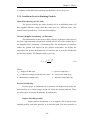
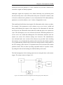
Transitions, (radiation or absorption) that an atom or ion can undergo can be
summarised using the following diagram:
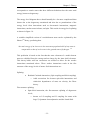
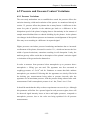
Figure 3.3: Illustration of possible transitions of electrons
(Composite drawn from many sources)
Where, from left to right we have:
•
bound-bound
•
free-bound (Avalanche)
•
free-free (Bremsstrahlung)
•
Ionisation from the ground state
•
Ionisation from an excited state
- 18 -
Chapter 3: Theory
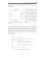
Once the plume is fully ionised light absorption is dominated by Bremsstrahlung
absorption. In this scenario the plume absorbs all or part of the incident radiation
and the energy provided is converted into internal energy of the plume. This
energy is consumed as hydrodynamic motion or radiated away as thermal
radiation. As mentioned, the plume rapidly expands away from the surface, but
this plume also remains confined to a channel formed by the incident light due to
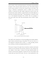
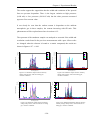
interaction of this light with the plume34. This phenomenon is commonly referred
to as a Laser-Supported Absorption Wave (LSAW). This wave propagates in
three zones, plume front, shock front and absorption front as shown in figure
3.334,70,71.
Figure 3.4: Schematic diagram of plasma propagation34
This LSAW can be divided into two classes depending on the incident irradiance,
optical density and internal energy of the plume. The first class, known as a
Laser-Supported Combustion Wave (LSCW), is a weakly absorbing subsonic
wave, the theory of which was formulated by Raizer in 197072.
The layers of cold gas in the plume front are heated by conduction and thermal
radiation from the absorption front until they themselves start producing their
own radiation. In this regime a fraction of the light absorbed produces the
chemical reaction and the propagation is limited to the laser beam channel, both
towards and away from the laser source. The wave is also optically thin so the
- 19 -
Chapter 3: Theory
laser radiation can still reach the surface. The velocity of the LSCW scales with
the square root of the irradiance and vanishes at critical irradiance61.
The second class of an LSAW is known as a Laser-Supported Detonation Wave
(LSDW). In this class the irradiance increases and in consequence there are
increases in the temperature, pressure and velocity of the absorption front. The
increased irradiance also results in a larger proportion of the beam flux being
absorbed, which in turn contributes to preheating and ionization, and ultimately
results in the dominating mechanism of plume expansion becoming compression
rather than conduction so that the plume front becomes optically thick. The
velocities increase and the wave becomes a supersonic shock wave. The plume is
also shown to propagate cylindrically along the beam path due to its mechanism
being supported by the laser beam.
At even higher irradiances the wave class changes to what is known as a LaserSupported Radiation Wave (LSRW), or breakdown wave. In this regime the
plasma itself is emitting enough radiation to enable the atmosphere in front of it
to become absorbing34. This couples the absorption zone to the plasma front. The
propagation of this wave relies on avalanche breakdown, with the avalanche first
developing at the focal point (region of highest flux) and then transferring that
propagation to areas of lower flux.
A one dimensional approximation study of velocities, pressure, temperature and
densities for all classes of laser supported waves has been carried out by Root73
in 1989 and a further study modelling ablation mechanisms, rates and analytical
considerations is reported by Bogaerts et al74.
All regimes will be altered with a change in ambient pressure producing a change
in the plume size. A higher pressure will slow down and confine the plume
whereas at low pressures there will be reduced trapping of the absorbed energy,
and as such a plasma lifetime decrease, but there will also be an increase in
ablation rate due to less plasma sheilding59.
- 20 -
Chapter 3: Theory
Review papers have been written by Bogaerts et al74 and Russo et al75, which
review the many models of the ablation process with varieties of laser and
sample parameters. Papers by Aguilera and Aragon76, Wood et al77, Iriarte et al78,
Capitelli et al79 and Gizzi et al80 also provide a good understanding of the
ablation/plume process within a LIBS plasma.
3.3 Breakdown (Plasmas)
‘After termination of laser pulse plasma loses energy and decays. Mechanisms
include recombination, radiation and conduction…’34
Plasmas produced by laser ablation will expand rapidly and show large density
and temperature gradients along the axis of the incoming beam. Typically,
plasmas produced in LIBS experiments initiate with high ionisation but after
recombination and relaxation the plasma becomes weakly ionised. Throughout
this process there is broadband background radiation due to Bremsstrahlung
radiation that decays early in the plasma lifetime. The plasma lifetime is only of
interest for LIBS experiments when it reaches the later stages, where the
recombination radiation is emitted.
LIBS plasmas should preferably be optically thin: an optically thin plasma is a
plasma in which the radiation that has been emitted escapes without noteworthy
absorption or scattering.
Ideally LIBS plasmas should have an elemental composition identical to that of
the substrate. This is not always the case due to the differing volatilities of the
constituent species of the substrate producing preferential ablation rates.
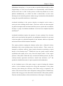
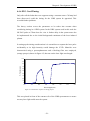
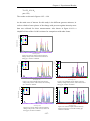
When analysing the intensity of different elemental spectral lines it has been
shown81 that there is a fractionation or matrix effect inherent in substrates
composed of a different matrix of elements.
- 21 -
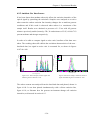
Chapter 3: Theory
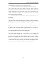
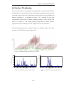
For example, figure 3.4 shows that, although the concentration of lead in the
sample is constant, its LIBS analysis shows an incongruent quantity, depending
on the matrix composition of lead and sand.
Figure 3.5: Graph showing matrix effect evident in samples
containing both sand and lead80.
Figure 3.5: Graph showing matrix effect samples containing both sand and lead81.
Many factors influence the degree of fractionation such as laser wavelength,
pulse duration and irradiance, fluence and atomic mass of the constituents, as
have been extensively studied by Russo et al75,82, Mao et al83, Figg and Kahr84,
Jeffries et al85, Eggins et al86, Gunther et al87,88 and Singh and Narayan89. It has
been indicated42 that matrix effects are less prominent at lower pressures, due to
the reduced proximity of the plasma species resulting in increased interaction
between the laser pulse and the sample.
In order to maximise stoichiometry all constituents should be completely
vaporised and removed. This can be done by ensuring the energy deposited into
the substrate is greater than the latent heat of vaporisation for all matrix
constituents. It has been noted by Ready90 that if the irradiance is <106Wcm-2
with microsecond pulse lengths then thermal effects will influence the process
allowing differential ablation, but for nanosecond laser irradiances >109Wcm-2
the ejected material should be close to the sample composition due to the thermal
properties no longer playing a major role. Bogaerts el al91 provide a review of the
laser ablation/plume process with varying models and sample parameters.
- 22 -
Chapter 3: Theory
When an electron undergoes a transition to a state of lesser energy it can emit a
photon. These photons produce spectral lines characteristic of the atom, ion or
molecule. Spectral lines emitted from a plasma have widths, shapes and
intensities that depend on the temperature, pressure and electron density of the
plasma. Therefore spectral lines can give information about the conditions in the
plasma itself. Lines that have been emitted from a ground level transition are in
most cases the strongest lines, known as resonance lines.
If a spectral line has changed from its expected value in some way this suggests a
perturbation in the medium. This could be a spectral line broadening or shifting
mechanism due to the plasma parameters. There are many broadening and shift
varieties, the most important in LIBS conditions being Doppler and Stark
broadening, described in section 3.3.1. The interference from these mechanisms
in LIBS plasmas will only be apparent if the spectrometer and detector system
has sufficient optical and spectral resolving power. Natural line widths can be
neglected in LIBS experiments as they are negligible when considering the
resolution of LIBS apparatus.
Table 3.1 illustrates Doppler and Stark widths for some lines of interest to LIBS
experiments: Table 3.1: Doppler and Stark widths from literature34, with electron densities of 1017.cm-3.
Element Wavelength
Atomic
Mass Temperature
(nm)
193.1
247.9
777.3
589.2
285.2
309.2
288.1
390.5
181.4
766.5
422.6
(K)
10000
10000
10000
10000
10000
10000
10000
10000
10000
10000
10000
C
C
O
Na
Mg
Al
Si
Si
Si
K
Ca
12
12
16
23
24
27
28
28
32.1
39.1
40
Doppler
FWHM
Stark width
FWHM
(nm)
(nm at 1017.cm-3)
0.004
0.0044
0.005
0.0072
0.014
0.0630
0.009
0.0314
0.004
0.0082
0.004
0.0520
0.004
0.0128
0.005
0.0234
0.002
0.0044
0.009
0.0830
0.005
0.0126
Table 3.1: Doppler and Stark widths from literature34, with electron densities of 1017.cm-3.
- 23 -
Chapter 3: Theory
A summary of the different broadening mechanisms will now be given:
3.3.1 Conditions Local to Emitting Particle
Natural Broadening, (no line shift)
The process whereby the same excited level in an individual atom will
have slightly different energy from that same level in a different atom. This
method can be described by a Lorentzian distribution.
Thermal (Doppler) broadening, (no line shift)
This phenomenon is due to the relative velocity of photons with respect to
the observing framework, the photons emitted will be red or blue shifted due to
the Doppler effect, producing a Gaussian profile. The distribution of velocities
within the plasma will depend on the plasma temperature, the higher the
temperature the greater the distribution of velocities and, as such, the broader the
spectral line emitted. The Doppler width is given by:
kT
λ D = λ0 2
mc
1
2
(3.6)
Where:
λD = Doppler width (nm)
c = speed of light (ms-1)
λ0 = Central wavelength of spectral line (nm)
m = mass of the atom (Kg)
k = Boltzmann constant (J/K)
T = absolute temperature (K)
Pressure broadening
Pressure plays an important role in plasmas, the higher the pressure the
more particles in a selected range which will affect the emitted radiation. There
are many types of pressure broadening, described here:
Impact (line shift possible)
Impact pressure broadening is, as it suggests, due to impact of the
emitting particle with other particles in its emission path. The more particles in
- 24 -
Chapter 3: Theory
its path the more impacts; thus this process is affected by the temperature and
density of the plasma. Broadened lines can be describes by a Lorentzian profile.
Quasistatic (line centre can be shifted)
This mechanism is due to nearby particles shifting the energy
levels and therefore the emission frequencies of the emitting particle, and thus is
dependent on plasma density. The line profile is affected by the distance between
the emitting particle and the perturbing particle92.
Linear Stark Broadening (can cause line shift)
This interaction is due to the interrelation of the emitting
radiation with an electric field. The shift in energy is linear with field strength
given by:
∆E ∝
1
r2
(3.7)
Resonance Broadening
This is the process whereby the emitting particle undergoes an
energy exchange with an identical particle. It can be described by a Lorentzian
profile and the relation:
∆E ∝
1
r3
(3.8)
Van der Waals Broadening
This process occurs when Van der Waals forces perturb an
emitting particle. This mechanism can be described in the centre of the plasma by
a Van der Waals profile and at the edges by the Lennard-Jones Potential93,94:
∆E ∝
1
r6
- 25 -
(3.9)
Chapter 3: Theory
3.3.2 Conditions Along Entire Emission Path
Opacity broadening
Plasma opacity is the re-absorption of an emitted photon. It can be so
great as to cause self reversal, whereby the centre of the emitted spectral line is
inverted. The re-absorption will be greater the more interactions there are along
the emission path. As such it is more apparent with emissions from the centre of
the plasma than those at the edges. This difference in re-absorption broadens the
spectral lines.
All of the above broadening mechanisms can be prevalent in a plasma, some in
isolation and some in combination. If these mechanisms are in fact working in
combination they can yield profiles which are a convolution of the individual line
profiles. Such a convolution is shown when a Gaussian and a Lorentzian
broadening mechanism are combined to produce a Voigt Profile. The Gaussian
dominating at the line centre and the Lorentzian dominating in the line wings95.
The purpose of LIBS analysis is primarily to discover the chemical composition
of a substrate. Qualitatively this is an easy procedure, shown by the presence of a
characteristic spectrum. To obtain quantitative results one must be able to
interpret the intensity of spectral lines, giving the number density of the species
in question. In order to undertake such a task one must determine the state of the
plasma, namely its temperature and density.
If a plasma displays thermodynamic equilibrium its temperature can describe
conditions of the plasma, such as distribution of particle speed and the relative
populations of energy levels. This state is rarely found and as such one can only
approximate with local thermodynamic equilibrium (LTE), applying to a local
sector rather than the whole plasma.
When a LIBS plasma extends to a LSDW or LSRW the energy in the plasma is
distributed across the whole volume, producing LTE at times several hundred
nanoseconds after the initial laser spark. This can be implied from work in this
- 26 -
Chapter 3: Theory
field addressed by Salzmann96 (1998), Griem97 (1997) and Sobelman98 et al
(1981).
If in fact LTE does exist, the relative populations of energy levels can be given
by the Boltzmann distribution.
Nj
N0
Where:
=
gj
U
exp
−E j
kT
with respect to the ground state.
(3.10)
Nj = population of the level Ej
N0 = Total species population
gj = Statistical weight of the level (2J + 1)
U = Partition function (statistical weight of the ground state)
Or:
Nj
Ni
=
gj
gi
(
exp
− E j − Ei
kT
)
for relative populations.
(3.11)
This information tells us that the ground state is most populated but as the
temperature increases the population moves to the excited states. This method
can be used to calculate the temperature of the plasma by measuring the
wavelengths and relative intensities of spectral lines, if their transition
probabilities and the statistical weights of the levels are known.
LTE within the plasma can also lead to a knowledge of the relative populations
among ion stages, if the electron density is known, by using the Saha Equation to
obtain temperature:
N (U ,0 )ne
=
N (U − 1,0 )
Where:
2 g (U ,0 )
3
− ∆E
mkT 2
g (U − 1,0 )
exp
2
2π
kT
N(U,0) = population of ground state of ion stage U
N(U-1,0) = population of ground state of ion stage U-1
- 27 -
(3.12)
Chapter 3: Theory
m = electron mass
ne = electron density
∆E = ionisation energy of stage U relative to stage U-1
This equation only holds for weakly ionised plasmas. In terms of relative
intensities:
I'
λg ' A' N (U )
= '
I λ gAN (U − 1)
(3.13)
The Saha equation describes the degree of ionization of this plasma as a function
of the temperature, density, and ionization energies of the atoms.
This method involves measuring the relative intensities of lines from different
ion stages and is known as the temperature of the ionisation equilibrium. The
results inform us as to which ionic species is dominating at which temperature
range. Increasing temperature causes higher ionic species to dominate.
Shown in figure 3.5 are results of the Saha calculation for nitrogen99. It can be
seen that only one or two ionisation stages need to be taken into account at
certain plasma temperature ranges.
Number of atoms in the r stage of ionization
and s state of excitation/Total
Figure 3.6:
Sahafactors
factorsapplied
appliedtotoNitrogen
nitrogen99
(pressure = 0.1 Pa)
Saha
(pressure=0.1Pa)
1.2
1.0
0.8
N(I)
N(II)
N(III)
N(IV)
0.6
0.4
0.2
0.0
0
5000
10000
15000
Temperature (K)
- 28 -
20000
25000
30000
Chapter 3: Theory
LIBS plasmas of irradiances of >108Wcm-2 have been shown34,100 to have
electron densities of N e ≥ 1016 cm −3 and temperature ranges of
kT ≥ 1eV at
several hundred ns after initiation, which classifies them as cold dense plasmas.
These electron densities will be highest at the initiation of plasma formation and
will decrease with plasma lifetime as shown in34.
Conversion of temperatures into electron volts is often undertaken in plasma
physics:
1eV
= T (kelvins )
kB
Where:
1.60 x10 −19
= 11604.50 K
1.38 x10 −23
(3.14)
kB = Boltzmann constant
If undertaking LIBS experiments at atmospheric pressure it is useful to note the
densities of molecular oxygen and nitrogen, the prevalent background species,
which are of the order of 2x1025 m-3. If LIBS is undertaken under different
pressure regimes it should be noted that plasma and background electron
densities will be orders of magnitude different.
Plasma properties such as line shape and width can provide us with much useful
information for LIBS analysis, such as quantative information on the electron
densities, electron temperature and relative concentrations of the elements
present.
- 29 -
Chapter 3: Theory
3.4 Spectroscopy
‘An optical spectrum consists of radiative transitions between stationary states
of an atom or molecule.’101
When an electron within an atom undergoes a transition to a state of lesser
energy it can emit a photon. These photons produce spectral lines of the atom,
ion or molecule, known as an emission spectrum.
Optical spectroscopy is the analysis of spectral lines emitted or absorbed from
atoms, ions or molecules and the use of this information to ascertain the identity,
structure and/or environment of such species. These lines represent the energy
levels of the emitting species.
Spectrochemical analysis is the search for characteristic emission line patterns
from an atom, molecule or ion. Analysis of their wavelengths, intensities, widths,
shifts and spectral distribution can provide further information. Analysis of the
emission spectra can be made quantative if one can determine the relative
intensities of such spectra to determine the abundance of that species in the
substrate.
Plasma spectroscopy can be used to analyse electron densities, temperatures,
pressures, velocities and relative abundances. A plasma’s physical properties can
be shown to affect the emission spectra in many ways. Studying these effects has
been covered in section 3.3, many of these effects are produced by line shifts and
broadening mechanisms as a result of plasma properties. A plasma’s properties,
such as temperature and electron density, can be determined from the emission
lines themselves.
The link between line wavelength and individual atom emissions/absorptions
was first discovered in 1860 by Kirchhoff and Bunsen. The foundations of
spectroscopy and atomic structure are covered in quantum mechanics.
- 30 -
Chapter 3: Theory
Quantum theory states that energy is quantised; it can only exist in discrete
packets of energy which satisfy the relation:
E = nhυ
Where
(3.15)
E = total energy
n = quantum number
h = Planck’s constant
υ = frequency of oscillations
The energy quantisation can be found for the one electron atom from the timeindependent Schroedinger equation. An energy level diagram for such a system
is shown below:
E
n
continuum
Energy above ground state
Ionisation
4
3
2
1
Ground state
Figure 3.7: Energy level diagram for one electron atom.
(composite drawn from many sources)
Although this theory has been developed for a one-electron atom, and as such an
energy level is only dependent on the quantum number n, the theory also holds
when applied to multielectron atoms but the energy of the system, due to the
levels having sub-levels and the electrons having spin, then depend on three
quantum numbers n, l and ml.
It can be seen that there are situations where a single energy value En can
actually depend on a few different configurations of energy in the system, this
- 31 -
Chapter 3: Theory
corresponds to atomic states that have different behaviour but the same total
energy, known as degeneracy.
The energy level diagram above should actually be a lot more complicated than
shown due to the degeneracy mentioned and also due to perturbations of the
energy levels from interactions such as electrostatic interactions, magnetic
interactions, nuclear mass/volume, and spin. This results in energy level splitting
as shown in figure 3.8.
A suitable simplified version of a multielectron atom can be explained by the
Hartree102 theory, predicting that:
‘the total energy of an electron in the outermost populated shell of any atom is
comparable to that of an electron in the ground state of hydrogen.’102
This prediction is based on the fact that the outer electrons of a multi-electron
atom are shielded from the strong nuclear charge by the inner shell electrons.
This theory holds well but corrections are needed to allow for the weaker
interactions mentioned above. These weaker interactions result in the fine
structure of the energy levels of atoms. Such interactions are:
Splitting:
•
Residual Coulomb interaction, (Spin coupling and Orbit coupling)
o Adds corrections for electron spin-orbit interactions and
relativistic dependences of mass on velocity, the Dirac
theory.
Fine-structure splitting:
•
Spin-Orbit interaction, the fine-structure splitting of degenerate
levels,
o known as LS coupling and JJ coupling for atoms with
large Z, Quantum electrodynamics and the Lamb Shift.
- 32 -
Chapter 3: Theory
Hyperfine splitting:
•
Interaction of the intrinsic magnetic dipole moment of the nucleus
and the magnetic field produced by atomic electrons.
o smaller than spin-orbit interactions by 3 orders of
magnitude
Figure 3.8: Influences on atomic energy levels103.
Figure 3.8: Influences on atomic energy levels103.
The Hartree theory yields information on ordering, according to energy, of the
outer filled subshells of multi-electron atoms.
Spectroscopic notation can be explained using standard notation, as shown:
For a boron atom:
5
B: 1s22s22p1
The principle quantum number n is represented by the integer before the letter;
the azimuthal quantum number, or subshell, is represented by the spectroscopic
notation in table 3.2; the superscript on the subshell designation specifies the
number of electrons which it contains; the superscript on the chemical symbol
specifies the number of electrons in the atom.
The filling of subshells is governed by the Pauli exclusion principle, whereby:
‘In a multielectron atom there can never be more than one electron in the same
quantum state’
- 33 -
Chapter 3: Theory
The first subshell may contain two electrons and not violate the exclusion
principle as one electron may have spin ‘up’ and one spin ‘down’.
Energy levels are often listed as wavenumbers (cm-1) where the ground state is
zero, allowing the wavenumber of a transition to be interpreted from the energy
level difference:
(
)
wavenumber , σ cm −1 =
∆E
hc
(3.16)
Derived from:
∆E = hυ
(3.17)
c = υλ
(3.18)
σ=
Where:
1
(3.19)
λ
E = Energy difference of two levels (J)
υ = frequency (Hz)
c = speed of light (ms-2)
λ = wavelength (nm)
The ionization energy, the energy required to remove an electron from the atom,
varies with the number electrons in the outer shells of each atom.
For example a noble gas, in which the p subshell is completed, is much harder to
ionize than an alkali which has a single weakly bound electron in an s subshell.
These alkali elements have correspondingly high chemical activity due to their
energetic favourability to interact with other elements to produce a more stable
arrangement.
An element’s chemical properties and its ability to interact with other atoms
depend on the number of electrons in the outer subshell of the atom, as these are
the electrons that govern the electric and magnetic fields of that element.
- 34 -
Chapter 3: Theory
Modern quantum theories are also able to give very satisfactory treatments of the
transition rates and selection rules observed in the measurements of the spectra
emitted by atoms.
3.5 Pressure Related Processes
LIBS measurements are influenced by the ambient conditions. Pressure alters the
plasma characteristics affecting the emission intensity, width and resolution of
spectral lines104-107.
In different pressure environments the temporal process of plume dynamics is
changed, because of a difference in the mean free path of particles in the
surrounding medium. There is also a discontinuity in the amount of mass ablated
from the sample due to these same changes in confinement of the plasma
volume.
Mean Free Path:
=
Where:
RT
2πd 2 N A P
(3.20)
ℓ = mean free path
R = universal gas constant = 8.31J/mol K
T = temperature
d = molecular diameter, nominal approximation value = 0.3nm
NA = Avogadro’s number = 6.0221x10²³mol-1
P = pressure
Leading to mean free path calculations of:
- 35 -
Chapter 3: Theory
160x103
Pressure
(mb)
1600
150x103
1500
68.1x10⁻⁹
101x103
1013
100.8x10⁻⁹
78x103
780
130.7x10⁻⁹
53x103
530
192.6x10⁻⁹
30x103
297
0.34x10⁻⁶
9900
99
1.03x10⁻⁶
5
5x10⁻²
2.04x10⁻³
0.03
3x10⁻⁴
0.34
1x10⁻⁵
10.21
Pressure
(Pa)
-3
1x10
400x10-6
Mean Free Path
(m)
63.8x10⁻⁹
-6
4x10
25.53
Table 3.4: Pressure values and corresponding mean free paths. (calculated
from equation 3.20)
This table shows pressure measurements in both the S.I. units of Pascal and
millibar, as millibar are the pressure units used in this work. From this table one
can see the huge difference in the mean free path of the particles that the plasma
volume is expanding into, from 64 nm to 26 m!
There may also be a change in the intensity of a spectrum due to the influence of
the surrounding medium. Such interference from the ambient gases may be due
to absorption or emission of spectral lines of interest. Much work has been done
in the area of low pressure LIBS systems104,105,107,108 but less has been covered on
high pressure systems106,109,110. However parallels can be drawn from papers on
Laser Emission Spectroscopy (LES) under high pressures in liquids. A paper in
this area reveals that “pressure has little effect on the early-stage plasma
evolution, but as the plasma cools, solution pressure begins to play a major
role”111
Low pressures result in reduced confinement of the plasma volume, allowing it
to dissipate more quickly and thus resulting in reduced excitation within the
plasma due to fewer collisions of the plasma species. In contrast to this, the mass
- 36 -
Chapter 3: Theory
of the ablated sample may increase due to the reduced shielding of the sample
surface by the plasma.
At pressures just below atmospheric pressure the plasma has been shown to be
larger than at atmospheric pressure108. These results show that the increase in line
intensity peaks at 1.3 kPa and then decreases beyond this point with no further
decrease below 0.4 Pa. The peak has been attributed to reduced confinement of
the plasma to the surface compared with that at atmospheric pressure and
increased mass ablation of the target, with the lack of further decrease being
ascribed to a steady state of ablation.
A different study undertaken at low pressures has shown greater than a 1 order of
magnitude increase in ablation rate when changing from atmospheric pressure
(101.3 kPa) to a pressure of 1.3 kPa105. This has been attributed to the reduced
shielding of the surface at these lower pressures.
The same study also showed a signal increase by a factor of 3-4 when reducing
the pressure from 78.6 kPa to 9.3 kPa105, and that continued reduction in pressure
resulted in a reduced line intensity. These results are expected due to plasma
dissipation in lower pressure regimes, but the loss in signal could also be due to a
misalignment or defocusing of the optics collecting the signal as the plasma size
changes.
At higher pressures one would expect the plasma confinement to increase
producing a small plasma volume. It has been shown in one account that this is
not the case due to the plasma having an extremely high pressure in the early
stages of its lifetime106. However, a contrasting investigation shows that the
plasma size does decrease with increasing pressure110.
There are documented accounts of high pressure environments causing some
spectral lines to broaden, occasionally resulting in self absorption due to
increases in confinement106. This would be expected with some spectra when
increasing the pressure due to the low lying upper levels in some species110. This
draws the conclusion that there is some increase in confinement, but it is
- 37 -
Chapter 3: Theory
minimised when the plasma is in initiation due to the plasmas internal pressures.
This argument is backed up by research undertaken by Arp et al106 (2004), stating
that “a steady state is reached at which increased pressure does not produce
decreased ablation.”
This study is also linked to discussions on plasma shielding under increased
pressures. It has been inferred that “above a certain pressure, once the plasma is
established, plasma shielding becomes so strong that further increases in the
pressure do not significantly increase shielding.” Having said that, these
measurements were done at very high pressures, 0.078 MPa – 9.1 MPa, and the
paper states that “The majority of change occurred as the pressure was increased
from atmospheric to 4.5 MPa”, so it is still of interest to study these affects in
our research.
In high pressure environments the ambient gas is also an important aspect. This
gas may absorb some of the emitted plasma species if the emission lies within the
absorption coefficient of the surrounding medium. The ambient gas may also
become excited itself, emitting at a possible wavelength of interest, (e.g. CH4
atmosphere interfering with possible C emissions from sample).
Data taken in a different piece of research done by Arp et al110(2004) shows that
in different pressure environments, when changing the delay time or laser power,
one observes a change in line intensity of these emissions but within the same
elemental spectra.
With all these factors to take into account when analysing LIBS in different
pressure environments one needs to consider the influences of; pressure;
temporal delays; power requirements and wavelength interferences.
- 38 -
Chapter 3: Theory
3.6 Power Related Processes
Power, or laser pulse energy, is important in LIBS research as it affects the
amount of ablated material and the plasma size in measurements. It is of
particular importance in this study as space driven applications often have power
limits, and a knowledge of the minimum power needed in order to produce a
reproducible plasma is crucial.
Measurements in lower pressures, carried out by Radziemski et al104, have
determined that the minimum energy at which a reproducible plasma can be
formed is 17mJ/pulse, and that there is a significant difference in results when
changing the pressure in the experiments. Another study, but for high pressure
systems, by Zane et al106 shows that increases in pulse energy from 30-50
mJ/pulse produce an increase in emission intensity. This research study will
examine those values and ascertain if this is also the case in the pressure and
gaseous environmental conditions of Titan, together with the changes that are
apparent in other pressure and gas regimes.
3.7 Gas Related Processes
The ambient gas in LIBS measurements plays an important role, as interference
from spectral lines and absorption of spectral emissions by the ambient gas can
occur. Titan has a methane nitrogen mix in its atmospheric composition.
Variations of these mixes were chosen for the study, together with pure gas fills
of nitrogen and methane. Nitrogen is known110 to be relatively inert and has few
atomic emission lines, minimizing interference. Methane is known to be
predominant on Titan in its atmospheric composition, precipitation and possibly
methane seas. It is of interest to study how much these gases and their absorption
at the higher pressures of Titan’s atmospheric conditions affect the LIBS plasma
and its emission properties.
Methane is known112,113 to have absorption bands in the infrared portion of the
electro-magnetic spectrum. These bands range from approximately 600+ nm.
- 39 -
Chapter 3: Theory
(619 nm, 727 nm, 890 nm being the lowest bands), the bands ranging from 750
nm can be seen in figure 3.8.
Figure 3.9: Absorption bands of methane from 750-940nm114
Figure 3.9: Absorption bands of methane from 750-940nm114
Methane is known115 to dissociate with the incidence of solar photons. Methane
plasmas contain many reactant products, species present incorporating115-119
many ions, radicals and molecules such as hydrocarbons, the most abundant
being: C2H6 (ethane) and C2H2 (acetylene), with others such as: C2H4 (ethylene),
C3H8 (propane), CH3 (methyl, free radical), CH2, CH, H, and H2.
Titan’s atmosphere contains predominantly nitrogen. The nitrogen radicals can
react with these methane radicals producing more complex materials such as
HCN (hydrogen cyanide), C2N2 (cyanogens), HC3N (cyano acetylene), C2H3CN
(ethyl cyanide) and HCN polymers. These products are known as tholins which
form the reddish-brown powder producing Titans haze.
- 40 -
Chapter 3: Theory
3.9 Optical Fibres
Many LIBS systems also make use of optical fibres (FO). A optical fibre utilises
the phenomenon of total internal reflection, whereby a ray hits the cladding at an
angle greater than the critical angle, θc, and as such is reflected back into the
core, as shown in figure 3.10:
ni sin θ c = nr sin 90
(3.24)
from Snell’s Law
Figure 3.10: Image of total internal reflection inside a optical fibre.
The acceptance cone angle for optical fibres of numerical aperture 0.22 is 25o26o.
Derived from:
Acceptance angle, a
Where:
sin a =
1
n0
n1 − n2
2
2
(3.25)
n2 = refractive index of cladding
n1 = refractive index of core
n0 = refractive index of external medium
if no = 1 then:
NA = sin a = n1 − n2
2
- 41 -
2
(3.26)
Chapter 3: Theory
3.10 Spectral Resolution/Diffraction
Spectrometers used in LIBS experiments utilize diffraction gratings to disperse
the light.
The grating equation for such a system is:
a sin θ = λm
(3.27)
Where:
θ = angle between normal to the
grating and the diffracted beam
a = ruled spacing
m = the integer of the order of the
Figure 3.11: Illustration of
diffraction parameters for a
grating.
maximum.
From this equation one can derive the angular dispersion, dθ/dλ:
dθ
m
=
dλ a cos θ
(3.28)
The ruled spacing is the reciprocal of the number of lines per unit length, so for a
150 grooves mm-1 grating, a is 6.7μm.
In most modern spectrometers ruled gratings are used, the angle of which is
adjusted to enhance a particular diffraction order120. These gratings are blazed
gratings as shown in figure 3.12:
- 42 -
Chapter 3: Theory
The angular positions of
the nonzero orders, θm ,
are determined by a, λ
and θi. The location of
the diffraction peaks is
governed by the blaze
angle, y.
The second illustration
shows the incident wave
normal to the plane of
the
blazed
grating:
reflection
θi = 0
Figure 3.12: Illustration of diffraction parameters
for a blazed grating.
For specular reflection:
θi – θr = 2y
Therefore the diffraction peak is at:
θr = -2y.
or:
θm = -2y,
in other words:
a sin (− 2 y ) = λm
- 43 -
(3.29)
Chapter 3: Theory
3.11 Detectors
The LIBS detection system is based on an Intensified Charged-Coupled Device
(ICCD). The ICCD works by coupling a CCD detector to a micro-channel plate
(MCP) to increase the gain in the system. The
MCP is closely related to a photomultiplier
tube, increasing the electron cascade as shown
in figure 3.13:
Photons incident on the photocathode are
absorbed and electrons are released, which are
then multiplied into a charge cloud by a cascade
in the MCP and finally are incident on the
fluorescent screen. The MCP can be gated with
Figure 3.13: An image intensifier tube
short time constants by controlling the voltage across the system.
The CCD works as an image sensor via the integration of an array of photoactive
capacitors. In reading the device each capacitor transfers its charge to a coupled
capacitor and so on until the charge is transferred to the last capacitor in the
system. This then transfers the charge to an amplifier to be converted into voltage
for the line by line reading of the array.
3.12 Timing
Timing considerations are extremely important in LIBS experiments. A gated
detector needs to capture the image of the plume when it displays the
recombination radiation emitted in the later relaxation stages; which is after both
the laser pulse and the background continuum have diminished, as shown in
figure 13.14.
- 44 -
Chapter 3: Theory
Figure 3.14: Illustration of timing requirements for LIBS experiments.
Typically the plume signal decays over an interval of one to several
microseconds, dependent on the energy deposited and the pressure regime, (with
reducing pressure the temporal process is shortened due to reduced confinement).
After approximately 1μs from the incident laser pulse the discrete spectral lines
begin to form from the recombination radiation emitted from the plume. This is
the spectral window of interest and as such the ICCD gate pulse needs to be
triggered within this period.
3.13 Limit of Detection
LIBS analysis brings with it many restrictions when undertaking qualitative and
quantative analysis. These limitations are commonly known as ‘Limits of
Detection’ (LOD) and can take many forms.
Apparent in every LIBS system are integral shot to shot variations, these can be
the result of many factors such as; laser intensity fluctuations, laser light
scattering due to surface effects and changes, geometrical and optical parameters,
ambient atmosphere attributes and dust particles. Also relevant are substrate
composition variations including, reflectivity changes, re-deposition from the
plume, integral composition incongruities and matrix effects.
These effects can be minimised but not eliminated. Known methods for reduction
of these influences are calibration, integration, analysis of ratios rather than true
intensities and background elimination.
- 45 -
Chapter 4: Development of LIBS
4. Development of LIBS
4.1 Experimental Apparatus
Salford University obtained a LIBS system in the summer of 2001 which was an
Acton Research Corporation, SpectraPro 500i, 0.500m, F/6.5, imaging triple
grating spectrograph , in a Czerny-Turner configuration [Appendix D]. The three
gratings incorporated are a 2400g/mm ruled grating blazed at 240nm a 600g/mm
ruled grating blazed at 1 micron and a 150g/mm ruled grating blazed at 300nm.
The spectral responses of the gratings are shown in [Appendix E].
The system also incorporates a Princeton Instruments Inc. PI-MAX Intensified
CCD (ICCD) camera with its intensifier photocathode working in the wavelength
range of 190 - 900nm. The synchronous operation of this camera and its
computer interface is accomplished via a ST-133 controller. To facilitate timeresolved measurements involving gating operations, the ST-133 has a built-in
Pulse Timing Generator (PTG) card, with 2ns width and 1.6ns delay gating
capabilities possible at a maximum repetition rate of 10Hz.
The camera uses a proximity focused microchannel plate (MCP) image
intensifier, which delivers light via a fused fibre-optic bundle, optically coupled
to a CCD array121. This intensifier acts both as an electronic shutter which is
controlled by the PTG and also as the gain medium for exposure. Integral to this
camera is the thermoelectrically cooled CCD detector with an active area of 26.6
x 6.6mm.
The software used to control the system’s gratings, PTG/ICCD and mirror and
also to capture the images was WinSpec/32122 with a Thermo Galactic™
GRAMS/32® interface. Also, the SpectraPro software provided with the
equipment was used to re-calibrate the EPROM in the system.
- 51 -
Chapter 4: Development of LIBS
The ablation source was a Continuum Surelite SLI – 10, Q-switched, Nd:YAG
laser, frequency doubled to run at 532nm, with a maximum power output at this
wavelength of 260mJ.
4.2 Laser Optimisation
The laser was not in operation when it was first commissioned, so a full
optimisation was undertaken.
Before the laser would operate a new flashlamp was purchased and installed, the
laser’s printed circuit board (PCB) was repaired. An assessment of any other
problems was then undertaken to optimise the laser output. This was done by
checking if the laser was free running, the power output was at full capacity with
optimum oscillator alignment, the beam shape was satisfactory and whether the
optics in the system were damaged.
The laser voltage was reset to read 1.06kV, (original 1.26kV). This enabled a
free running verification. This optimisation was done with an oscilloscope set up
to take readings from a photodiode circuit incorporating a silicon photo-detector
(bpx65) with a rise time of ~3.5ns.
Readings were taken by imaging a business card placed between the pockel cell
and the ¼ wave plate while the shutter was open. The curve on the oscilloscope
was analysed, free running being apparent when spikes showed in the output
curve.
Voltage readings were scanned, checking for free running spikes apparent in the
oscilloscope reading. After full characterisation had been fulfilled the laser
voltage was set to 1.38kV.
The beam shape was checked using photographic paper and the alignment
adjusted accordingly.
- 52 -
Chapter 4: Development of LIBS
Lastly the beam profile was analysed. Initially this was attempted using an image
of the beam profile as shown in figure 4.1:
Figure 4.1: Setup and image of beam profile capture using CCD camera
This was unsatisfactory because, in order to capture the image with the CCD
available, the beam needed to be diverged and attenuated. This changed the beam
profile and added aberrations to an unknown extent and as such this could not be
used as viable information. Consequently a photodiode was set up as shown:
Figure 4.2: Setup and circuit diagram of beam profile capture using photodiode
- 53 -
Chapter 4: Development of LIBS
The beam profile was taken using voltage readings from the photodiode. The
results are shown here:
YAG Beam Profile
YAG Beam Profile
16.00-18.00
14.00-16.00
12.00-14.00
10.00-12.00
5.00-10.00
6.00-8.00
4.00-6.00
2.00-4.00
18.00
16.00
14.00
12.00
10.00
8.00 Intensity
6.00
4.00
2.00
0.00
51
44
37
x-direction
(mm)
30
44
48
52
56
60
27
60
58
56
54
52 y-direction
50 (mm)
48
46
44
15.00-20.00
42
40
10.00-15.00
40
x-direction (mm)
30
33
36
39
42
45
48
Intensity
51
8.00-10.00
y-direction
(mm)
0.00-5.00
Figure 4.3: Charts showing beam profile from photodiode capture, the different
colours represent the beam intensity
As can be seen, the profile was far from ‘true’ Gaussian. To combat this, the less
intense section of the beam was masked out to produce a near homogeneous
beam output at the high intensity range.
Once the laser had been fully reconditioned the new spectrometer system was
evaluated. This was initially done using known wavelength emissions from a
constant source; a cadmium (Cd) lamp, with the wavelength emissions;
361.0508nm, 479.9912nm and 508.5822nm used for calibration.
- 54 -
0.00-2.00
Chapter 4: Development of LIBS
4.3 Light Coupling Optics
An optics system was developed to couple the light to the spectrometer. This
delivered the light from the Cd lamp, (and subsequently the laser ablated plume),
to the spectrometer at an observed focal length of 0.5m. The software used to
optimise this lens setup was OSLO LT developed by Sinclair Optics123. After
careful consideration of the possible parameters, using the lenses available, the
setup shown in figure 4.4 was finalised. The lens database, and OSLO
parameters are attached in [Appendix F].
Figure 4.4: Light coupling optics lens setup diagram
This setup takes parallel light into the spectrometer at a distance of 89mm but
with an observed distance of 500mm. The incident light first has to be
collimated. This is done using a simple convex lens placed in front of the above
lens system, set at the focal point of the lens from the light source.
- 55 -
Chapter 4: Development of LIBS
4.4 System Malfunction Evaluation
The LIBS suffered from a number of malfunctions that had to be addressed
before the experimental work could commence. This proved to be very time
consuming.
However, as each problem was successively removed, the evaluation of
subsequent problems became easier. Unfortunately, it was approximately 2 years
before all the problems had been resolved. While this evaluation and solution of
the problems was inevitably time consuming, a full appreciation of the
capabilities and limitations of the system was acquired over the period. The
problems, together with their solution, are detailed below.
4.4.1 EPROM:
The EPROM was programmed with an incorrect code which caused faulty return
settings of the grating turret and incorrect software readings indicating which
grating was currently active. For example, when the turret was on 2400g/mm the
software read that it was on 150g/mm, the actual grating that was active was
ascertained by the spectral window present in each capture.
This problem was solved by using SpectraPro software in Terminal Mode and
HyperTerminal, available from Windows98. The status of the EPROM was read
using the mono-eestatus dialogue box within HyperTerminal. These settings
were found to be faulty and so the EPROM was restored by ‘flashing’ it with
original factory settings.
4.4.2 Stepper Motor:
The stepper motor problems were highlighted when erroneous wavelength
readings were observed, as they were shifting beyond acceptable tolerances. The
accepted wavelength reproducibility of each grating is stated in the system
specification [Appendix D]. The wavelength reproducibility fell outside these
accepted values. For example, a shift of 12nm occurred on the 150g/mm grating
where the specification for this grating quotes a wavelength reproducibility of +/-
- 56 -
Chapter 4: Development of LIBS
0.4nm. These faults highlighted a problem and a new stepper motor was
installed. The data is shown in the tables below:
Table 4.1: Table showing wavelength reproducibility errors, Grating 2400g/mm.
Wavelength reproducibility = +/-0.025nm, resolution for ICCD based on 4 pixels = 0.085nm
Test
Peak
wavelength
value
576.9805
576.5762
576.9935
576.5762
576.5892
576.5761
576.7308
576.9935
576.9672
576.5975
576.9670
Number
2
3
12
15
18
28
31
60
64
67
68
Wavelength change
(with previous test
number)
-0.4043
0.4173
-0.4173
0.013
-0.0131
0.1547
0.2627
-0.0263
-0.3697
0.3695
Table 4.2: Table showing wavelength reproducibility errors, Grating 600g/mm.
Wavelength reproducibility = +/-0.1nm, resolution for ICCD based on 4 pixels = 0.34nm
Test
Number
0
4
13
16
23
33
39
51
Peak
wavelength
value
579.1869
576.4671
579.2855
576.4638
576.6306
576.6302
576.6302
579.5115
Wavelength change
(with previous test
number)
-2.7198
2.8184
-2.8217
0.1668
-0.0004
0
2.8813
Table 4.3: Table showing wavelength reproducibility errors, Grating 150g/mm.
Wavelength reproducibility = +/-0.40nm, resolution for ICCD based on 4 pixels = 1.36nm
Test
Number
1
5
14
17
24
34
40
52
Peak
wavelength
value
545.3674
534.6346
545.9348
533.613
533.9536
533.613
534.2941
546.6258
Wavelength change
(with previous test
number)
-10.7328
11.3002
-12.3218
0.3406
-0.3406
0.6811
12.3317
- 57 -
Chapter 4: Development of LIBS
4.4.3 Mirror:
It was found that the diverting mirror on the entrance slit was not always
returning to the settings set in the software, (front or side position). This was
ascertained when captures that should have produced a strong signal output were
only producing noise. After all other possibilities were ruled out it was deduced
that the mirror must not be returning to its correct alignment. The spectrometer
was opened up and it was found that the returning spring had become detached,
this was re-attached and no further problems manifested themselves.
4.4.4 PTG Cable:
The manufacturers discovered a problem with all their serial cables which
relayed the signal from the spectrometer camera to the PTG card. They were all
recalled and replaced.
4.4.5 Software:
There were many other WinSpec software problems that became apparent while
running tests to optimise the system. Each was reported to the manufacturers and
most were corrected with the advent of new software. Some of these problems
are listed below, a selection of sweeps are detailed in [Appendix G]:
Continuous cleans
With continuous cleans set ‘on’ there was no signal able to be
captured, (with continuous cleans ‘off’ the system worked
satisfactorily). A solution was not provided and as such the
system cannot be run with continuous cleans on.
Burst mode
This facility is available to take multiple shots from a single
trigger pulse, allowing analysis of the plume temporally. This
mode never worked and as such this facility was unavailable.
View width/delay sequence
This button is meant to show the user the width and delay
sequence for sequential timing. Each time it was pressed the
software crashed. This was also true if one attempted to save these
values to file. This was resolved by reverting to a previous version
of the software.
- 58 -
Chapter 4: Development of LIBS
4.4.6 PTG Card/Timing:
Only after all the faults that were apparent using a constant source Cd lamp had
been discovered, could the timing for the LIBS system be appraised. This
revealed further problems.
The theory section covers the parameters to be taken into account when
considering timing in a LIBS system. In the LIBS system used in this work the
Nd:YAG pulse at 532nm lasts for ~6ns. A further delay in the system must also
be implemented due to the initial background continuum of the laser induced
plasma.
In setting up the timing considerations it is essential not to capture the laser pulse
accidentally as its high intensity would damage the ICCD. Materials were
characterised using a spectrophotometer and a blocking filter was employed,
(orange perspex) shown in figure 4.5, that cut out the laser light wavelength:
100
90
% Transmission
80
70
60
50
40
30
20
10
0
200
300
400
500
600
700
800
900
Wavelength (nm)
Figure 4.5: Transmission response of orange perspex.
This was placed in front of the entrance slit of the LIBS spectrometer to ensure
no stray laser light could enter the system.
- 59 -
Chapter 4: Development of LIBS
The timing for the system was originally set using a Pulse Generator in the
following setup:
This setup however was found
not to work satisfactorily. The
laser
fired
correctly
when
receiving an input pulse, but the
ST-133 controller did not send
the signal to the camera. It was
found that the controller was not
in fact receiving the pulse as
there
Figure 4.6: Schematic of the system timing using pulse
generator
was
an
impedance
mismatch.
In order to match the output of the pulse generator, (15V), to the external sync
input, (5V), of the ST133 controller an in-house impedance matching circuit was
needed. This was developed using Electronics Workbench124 software as a guide.
The circuit below was devised utilizing a TL071CP fast Op-Amp. (Originally an
LM741 Op-Amp was used but this was found not to respond fast enough to the
10Hz input signal.)
Figure 4.7: Circuit diagram of impedance matching circuit
- 60 -
Chapter 4: Development of LIBS
With the new system the camera was now able to capture a signal, but this signal
was found to consist only of noise. This was thought to be a result of the timing
in the system. A delay could be introduced via the software for the PTG, but no
matter how much this delay was varied, no LIBS signal was captured.
After careful investigation it was found that the inherent delays in the system
itself, (such as device and wiring delays), were much larger on the controller side
of the system layout than on the laser side, causing the camera to capture the
event after the LIBS signal had completely died away. A timing circuit was
developed to produce a delay on the laser side of the system. It was hoped that
the PTG software should then be able to introduce a sufficient delay to match the
camera shot to the plume output. The following circuit, figure 4.8, was
formulated which produced a delay of 49.4ms
Figure 4.8: Circuit diagram of delay circuit
The system was setup accordingly, as shown in
figure 4.9:
Timing was calculated using:
Cable Delays = 1.5ns/ft = 4.92ns/m
Speed of light = 3x10⁸ ms-1
Figure 4.9: Schematic of the system timing
using delay and impedance circuit.
- 61 -
Chapter 4: Development of LIBS
After exhausting a wide range of PTG software delay possibilities and still
getting no LIBS signal the circuit was re-analysed and it was found that the
capacitor in the circuit did not respond quickly enough to the input signal. This
capacitor was replaced but unfortunately this still did not produce a LIBS
capture.
It was decided to remove all unknowns from the system
to ascertain if any of the faults were due to a
malfunction in the hardware or PTG software, as the
schematic shows in figure 4.10.
Figure 4.10: Schematic of the system timing,
showing redundant parts of system to be
removed for calibration.
Figure 4.11: Schematic of the system timing,
showing setup with external timing box.
The PTG settings were cross referenced
with an external timing box connected to
a light emitting diode (LED) emitting at
369 nm, the schematic is shown in figure
4.11.
This box was set to turn on the LED
after a 1s delay from its trigger-in and
keep it on for 0.5s, (timing latency =
±1μs).
The pulse generator sends a
trigger to the timing box and a
concurrent signal to the ‘external trigger
in’ on the back of the PTG card, via the
impedance circuit.
With the setup shown in figure 4.11 there was still no signal captured. The
manufacturers were informed and they took the PTG card and repaired it. This
- 62 -
Chapter 4: Development of LIBS
still did not solve the problem, so a new controller was provided. With the new
controller a signal was finally captured.
Although a signal was captured it was found, following cross referencing with
the known delay time on the LED and the delay time on the PTG software, that
in fact the software had a problem. It was evident that the PTG width and delay
parameters, set on the software, were 3 orders of magnitude in error.
This manifested itself when observing the file information after a shot was taken.
For example if the parameters on the software were set to 1msec, (width and
delay) and following the capture of the image the file information for that shot
was observed, the information showed that the width and delay were captured at
1μsec. This discrepancy was cross referenced with the LED timing known to be
correct and it was found that although the file information obtained after the
capture was correct. the software settings were incorrect. The manufacturers
were informed and a new version of the software was provided. After checking
this software it was found that the problem still existed, but after further analysis
it was found that the problem only existed when using repetitive timing mode on
the PTG settings of the software. If sequential mode was used instead no similar
problem existed. This was done by setting sequential mode in ‘repetitive’ mode,
by setting the start and end settings on width and delay as the same.
The final arrangement for the timing system was set using the laser as the master
trigger. The setup is shown in figure 4.12:
Figure 4.12: Schematic of the final arrangement for the timing setup of the LIBS system
- 63 -
Chapter 4: Development of LIBS
The laser sends a signal to the controller via its fixed sync out, the laser fires
108.4±1125 ns after the fixed sync out signal leaves. The laser light travels to the
material under test (MUT) in 13.2ns. The signal takes 22.63ns to travel from the
laser fixed sync ‘out’ to the external sync ‘in’ on the controller. There are
internal delays in the controller, PTG and camera system which take 62.26ns.
The software delays the ICCD camera shot until required. The light from the
plume takes 10.7ns through the optical fibre of refractive index 1.6 to the
spectrometer entrance slit, the light then takes 1.67ns to travel from the entrance
slit to the ICCD.
The delays are summarised here:
Light travel to Camera = 134ns
Signal travel to Camera Capture (plus variable delay) = 85ns
Figure 4.13: Schematic of the final arrangement for the timing setup of the LIBS system,
with inherent delays shown.
- 64 -
Chapter 4: Development of LIBS
4.5 Grating Efficiencies
Following the system timing setup described above, a check of the system’s
gratings efficiencies was undertaken and dummy’s guides were written on the
LIBS system’s operation and setup parameters.
Intensity information at four wavelengths was obtained for each grating using
spectral emissions from a mercury lamp, as shown in figure 4.14. This data was
cross referenced with the National Institute of Standards and Technology126
Intensity (arbitrary)
Thousands
(NIST) values.
26
21
2400g/mm, 240nm Blaze
600g/mm,1um Blaze
150g/mm, 300nm Blaze
NIST Intensity
16
11
6
1
365.015
404.656
435.833
546.074
Wavelength (nm)
Figure 4.14: Intensity versus wavelength chart for
mercury lamp emissions obtained from spectrometer
captures and NIST values.
The trend differences are due to the grating efficiencies and should be taken into
account when analysing results.
80
2400g/mm, 240nm Blaze
600g/mm,1um Blaze
150g/mm, 300nm Blaze
70
Efficiency (%)
60
50
40
30
20
10
0
360
380
400
420
440
460
480
500
520
540
Wavelength (nm)
Figure 4.15: Grating efficiencies versus wavelength
- 65 -
560
Chapter 4: Development of LIBS
Taking into account the percentage efficiency of each grating when plotting the
intensity of each spectral line, the intensity versus wavelength chart fits more
Intensity (arbitrary)
Thousands
closely with measured NIST values.
14
12
2400g/mm, 240nm Blaze
600g/mm,1um Blaze
150g/mm, 300nm Blaze
NIST Intensity
10
8
6
4
2
0
365.015
404.656
435.833
546.074
Wavelength (nm)
Figure 4.16: Intensity versus wavelength for gratings
corrected for their efficiency wavelength response.
As can be seen, the 600g/mm grating in this wavelength bandwidth is not
efficient, and as such was ruled out for future experiments. The optimum gratings
to use for the wavelength range to be investigated are the 150g/mm and
2400g/mm.
4.6 Dummy’s Guides
A number of simple manuals have been written to facilitate a new user’s
operation of the LIBS system – the so-called “dummy’s guides”. The first
dummy’s guide to be written was Basic Spectrometer System Use, [Appendix
H]. A manual was written for the use of the spectrophotometer, [Appendix I] and
one was also written for the Conversion from WinSpec to Grams & Multifile
Building, [Appendix J].
Together with the dummy’s guides, computer programs were written by the
author of this thesis in order to analyse the spectral lines obtained and match
them to elements’ spectral emissions. This was done using an astronomical
catalogue and data table provided by NASA’s now terminated Astronomical
Data Centre (ADC). This catalogue [Appendix K] was obtained from their now
discontinued ftp site: ftp://adc.gsfc.nasa.gov, in .dat format, last updated by Paul
- 66 -
Chapter 4: Development of LIBS
Kuin [NASA/ADC] 07-Oct-1996. It appears that this information can possibly
now be obtained from http://www.maa.agleia.de/Cat/sac_v_2.html#list quoting
that the original data was: 6016 Line Spectra of the Elements (Reader, Corliss
1980-1981), see also catalogue 6086.
The format of the data was changed and prepared for use. A software program
was then written in Pascal, (attached in [Appendix L]), to take spectral lines and
search the database for matches, dependent on the wavelength accuracy for the
grating which obtained the data.
After successive use of this program it became apparent that an update was
needed. The process of acquiring the information was too laborious: it involved
running the Pascal program, which then put the data into text files. Following
this the text files needed to be compiled into one file, usually in Excel.
To facilitate quicker analysis a new database was set up in Access, (attached in
[Appendix M]), which had queries to interrogate the data. This also output the
spectra data into text files, which would need to be compiled into one file for
viewing, but it did interrogate the data much more quickly than the previous
Pascal program.
Lastly this database was advanced with Visual Basic for Applications (VBA)
programming, (attached in [Appendix N]), to enter the data directly into Excel on
separate sheets in one workbook. This program saved much time with analysis
and so many other programs were written to assist the analysis process. All
programs are listed here, and the full code is added to the appendices.
VBA Programs:
VBExcel Modules
A single workbook was used to contain all relevant programs and
macros used for data analysis, correlation and formatting. A selection are added
to [Appendix O].
- 67 -
Chapter 4: Development of LIBS
Pascal Programs:
Wavefini
Original program built to interrogate the spectra at wavelength
and grating specifications, attached in [Appendix L]
Peakshot
Program built to analyse the intensity of selected emission peaks,
attached in [Appendix P]
Relstddev
Pascal program used to find average, standard deviation and
relative standard deviation of a dataset, attached in [Appendix Q]
There was also a dummy’s guide written to facilitate the use of some of the
programs that are used in depth profiling, attached in [Appendix R]
- 68 -
Chapter 5: Development of Pressure Apparatus
5. Development of Pressure
Apparatus
5.1 Experimental Apparatus
In order to facilitate the application of LIBS in different pressure environments
suitable high pressure/vacuum apparatus (HPVA) was developed from existing
hardware. The main experimental chamber consisted of a base unit and chamber,
as shown in the working drawings shown as figure 5.1.
5.2 Dome Window
The dome had an optical window. Its transmission curve was analysed in a
spectrophotometer to ensure satisfactory transmission for the laser input (532
nm), shown in figure 5.2:
Figure 5.2: Chart showing transmission curve for the HPVA dome.
- 69 -
Figure 5.1 Working drawings of HPVA chamber
- 70 -
Chapter 5: Development of Pressure Apparatus
5.3 Sample Stage
A sample stage was developed from an old Scanning Electron Microscope
(SEM) stage, which originally worked in a horizontal position. The capability to
run vertically was solved by changing the stage’s runners and adding a constant
force spring of force 2N, kindly donated by Kern-Liebers127.
A bracket was designed and developed128 to couple the adapted SEM stage to the
HPVA with feedthroughs for the micrometer movement rods of the stage, as
shown in figures 5.3 & 5.4.
Sample
Holder
Constant Force
Spring
Coupling
Bracket
Stage
Movement
Feedthroughs
Figure 5.3: Image to show
micrometer feedthroughs of
sample stage on the HPVA
Figure 5.4: Image to show sample stage and coupling
bracket
- 71 -
Chapter 5: Development of Pressure Apparatus
5.5 Optical Fibre
In order to couple the output from the laser plume to the external spectrometer
optical fibre coupling was used.
This consisted of a UV-VIS optical fibre bundle, 2 metres long with a quartz core
transmitting at 190nm to 1100nm. It contains a single row of 200 micron fibres
terminating in 10mm diameter ferrules, as shown in figure 5.5.
Figure 5.5: Image of configuration of
fibre bundle at the spectrometer end
An imaging fibre adapter was also included, designed specifically for imaging
spectrometers. “The all-reflective design eliminates chromatic aberrations and
the aspheric mirror cancels astigmatism, allowing precise imaging of fibres at
the spectrograph entrance slit”129.
To pass the optical fibre through the HPVA chamber wall, a unique feedthrough
was designed, as shown in fig 5.6:
- 72 -
Chapter 5: Development of Pressure Apparatus
Figure 5.6: Drawing of optical fibre feedthrough, courtesy of John Cowpe and Richard Pilkington
The optical fibre was set up to directly image the plume as shown in images 5.7
& 5.8, particular attention being paid to the angle of the optical fibre, to ensure it
imaged a good cross section of the plume
Figure 5.7: Image showing alignment of fibre end
Sample
Optical fibre
feedthrough
Fibre end
Figure 5.8: Image showing optical fibre
feedthrough
- 73 -
Chapter 5: Development of Pressure Apparatus
5.4 Vacuum Apparatus
The vacuum apparatus was used for measurements below roughing pressures of
5x10⁻² mb (the units of pressure given throughout this work are those taken from
the gauges used) was set up as shown in figure 5.9. All other pressure
measurements were taken using the setup shown in the next section.
Figure 5.9: Schematic of vacuum apparatus setup
- 74 -
Chapter 5: Development of Pressure Apparatus
5.5 General High Pressure/Vacuum Apparatus
The vacuum system for the majority of measurements was set up as shown in
figure 5.10, allowing capability to run the system at high pressure or vacuum.
Figure 5.10: Schematic of high pressure/vacuum apparatus setup
- 75 -
Chapter 5: Development of Pressure Apparatus
5.6 Leak Detection and Calibration
Both systems were leak checked before experimental work commenced. The
Mass Flow Controllers (MFC) were calibrated against accurate Transfer
Standards as shown in figures 5.11 & 5.12 Results are presented in figures 5.13
& 5.14:
Calculated Flow
Actual Flow
100
20
90
18
80
16
70
14
60
50
12
10
40
8
30
6
20
4
10
2
0
Actual Flow
Calculated Flow
22
Flow
Flow
110
0
15
25
35
45
55
65
75
85
95
105
2
4
6
8
Setpoint
10
12
14
16
18
20
Setpoint
Figure 5.11: Calibration of 100sccm MFC
Figure 5.12: Calibration of 20sccm MFC
Time (mins)
0
1.6
5
10
15
20
25
5.0E-03
4.5E-03
1.5
4.0E-03
3.5E-03
Pressure (mb)
Pressure (b)
1.4
1.3
1.2
3.0E-03
2.5E-03
2.0E-03
1.5E-03
1.1
1.0E-03
1
5.1E-04
5.0E-06
0.9
0
10
20
30
40
50
60
Time (mins)
70
Figure 5.14: Leak rate of vacuum apparatus
Figure 5.13: Rate of fill of HPVA
In high pressure experiments, rather than using and running the possibility of
damaging the vacuum gauges, the Bourdon high pressure gauge, as shown in
figure 5.15, was calibrated for its repeatability and usefulness at determining
pressures below atmospheric.
- 76 -
30
35
Chapter 5: Development of Pressure Apparatus
1600
Calibrated Pressure (Torr)
1400
1200
1000
800
600
400
200
0
-1.5
-1
-0.5
0
0.5
1
Gauge reading pressure (b)
Figure 5.15: Image of Praxair
Bourdon gauge
Figure 5.16: Average of three sets of measurements for
calibration of the Bourdon gauge when used at pressures
below atmospheric
It was found, as shown in figure 5.16, that the gauge showed good repeatability
in this range and was utilised in experiments where high pressure and vacuum
analysis was undertaken in one sweep.
5.7 Optical Bench Layout Incorporating Vacuum
Chamber
The optical bench was setup as shown in figure 5.17, As can be seen in this
setup, the optical coupling system, described in section 4.3, was replaced with
the optical fibre system outlined above.
Figure 5.17: Schematic of optical bench setup
- 77 -
1.5
Chapter 6: Experimental Results
6. Experimental Results
6.1 Development of Experimentation Techniques
6.1.1 General Experimental Parameters
All experiments unless otherwise stated were undertaken with a power 0.29 W
giving a laser pulse power of 57 mJ/Pulse. To compensate for the loss of signal
achieved with reducing power, the fluence in the pressure experiments was set
near to the maximum obtainable value of 14 mJ.cm-2. Although this does have
the drawback of poor shot to shot stability as discussed previously, it does
increase the signal which is a requirement when compensating for the reduced
intensity with reduced pressures.
All delays unless stated otherwise were set to 0.6 μs as this has been found, as
shown in chapter 10, to be a suitable delay to obtain a signal under all pressure
regimes investigated. It is important to bear in mind that a signal will show a loss
at higher or lower than atmospheric pressures due to the delay not being
optimised for these settings.
Widths were set at 0.8 µs after analysis of the optimum setting for the
experiments undertaken, described in section 6.6.
- 78 -
Chapter 6: Experimental Results
6.1.2 Characterisation/Calibration
Characterisation of the LIBS system’s capabilities, calibration of these
capabilities and error analysis was undertaken once the system was working
within acceptable tolerances. Calibration was undertaken using a cadmium (Cd)
and/or mercury (Hg) lamp as a reference source. Shown here in figure 6.1 are the
intensity fluctuations of the Cd lamp over time, the marker curves showing in red
every 5 shots.
Figure 6.1: Graph showing fluctuations in cadmium lamp intensity over time
Also shown are three representative calibration plots, figures 6.2, 6.3 & 6.4,
taken with a mercury lamp using each grating. Each spectrum obtained was
7
12
11
Hg (I) 576.959
5
4
3
2
Hg (I) 579.066
6
10
9
8
7
6
5
1
0
400
13
Hg (I) 579.066
8
Intensity (arbitrary)
9
Hg (I) 576.959
Hundreds
10
Hg (I) 546.073
Intensity (arbitrary)
Thousands
within the error for that grating.
450
500
550
600
650
700
Wavelength (nm)
750
4
540
550
560
570
580
590
600
Wavelength (nm)
Figure 6.2: Calibration using mercury lamp,
150grooves/mm grating
Figure 6.3: Calibration using mercury lamp,
600grooves/mm
- 79 -
610
16
14
Hg (I) 579.066
Hg (I) 576.959
Intensity (arbitrary)
Hundreds
Chapter 6: Experimental Results
12
10
8
6
4
571
573
575
577
579
581
583
Wavelength (nm)
Figure 6.4: Calibration using mercury lamp,
2400grooves/mm
Following calibration, a comprehensive spectral line search was commenced
using several different samples; namely, dysprosium, lead, zirconium, indium,
silicon, copper, carbon, glass and tin. These results were found to be in good
agreement with NIST data of spectral lines, verifying the LIBS setup and
calibration.
An example using a copper sample is shown. All lines fitted with NIST data
Cu (I) 515.324
35
15
10
Cu (I) 465.112
20
Cu (I) 427.511
25
Cu (II) 451.605
30
Cu (I) 521.820
40
Cu (I) 359.913
Intensity (arbitrary)
Thousands
results within the margin of error; some of the main emissions are marked.
5
0
300
350
400
450
Wavelength (nm)
Figure 6.5: Copper emission spectrum
- 80 -
500
550
600
Chapter 6: Experimental Results
6.1.3 Optimum Fluence
Analysis was undertaken to ascertain the optimum fluence value for
experimentation. This value is known to be critical34 in LIBS measurements and
is often quoted as lens to sample distance or LTSD.
High intensity output was considered in conjunction with shot to shot variation of
this intensity. Varying intensities of different elements’ and compounds’ spectral
emissions at set distances from the focal point of the lens were analysed. These
were cross referenced with their fluence values which show, in figure 6.6, an
asymptotic relation to a sample’s distance from focal point.
Figure 6.6: Chart showing fluence at varying distances from the focal point of the final lens
An optimum distance, (i.e. fluence), was then ascertained considering the signal
output against losses incurred in shot to shot stability. In order to test this
parameter fully, many samples were tested encompassing: silicon, dysprosium,
lead, copper, indium, selenium, and copper indium diselenide (CIS) (both thin
film and polycrystalline). Shown in figure 6.7 are the results obtained from the
constituents of CIS, and the compound CIS itself, both analysed to ensure that no
significant changes occur when an element is bound to a compound.
- 81 -
Figure 6.7: Emission intensity versus distance from focal point for CIS and its constituents
- 82 -
Chapter 6: Experimental Results
It was found generally that at higher fluence values a higher intensity of signal is
obtained, but this comes with the drawback that the standard deviation of this
intensity is large. It is therefore more prudent to choose a lower fluence value to
ensure that the shot to shot stability is more uniform.
As such, samples in future experiments will generally be placed at approximately
6-7mm in front of the focal point of the final convex lens. Although positioning
of the sample behind the focal point does appear to be more experimentally
sound, the results do not take into account the losses incurred due to the laser
‘spark’ as the power is high enough to break down the air at the focal point. This
in itself would interfere with LIBS measurements and for this reason positioning
behind the focal point was ruled out.
- 83 -
Chapter 6: Experimental Results
6.1.4 Imaging
Imaging mode was utilised in order to establish the full height of the slit image
on the chip. This parameter is useful for the possible manufacture of an in-house
optical fibre coupler.
A cadmium lamp was imaged using each grating, an example image from the
150grooves/mm grating is shown in figure 6.8:
Figure 6.8: Spectrometer image of cadmium emission lines
The input from the source was blocked at the entrance slit of the spectrometer
with a vernier attached to two blocks above and below the slit. The image height
in pixels was cross referenced with the vernier reading on the blocks. An
observable image of 6.5 mm within the slit height was established:
300
Imaged Height (pix)
250
200
150
100
50
Full slit height ~0.65cm
0
0.40
0.60
0.80
1.00
1.20
1.40
Vernier Reading (cm)
Figure 6.9: Imaged size of spectrometer entrance slit versus actual vernier reading
- 84 -
1.60
Chapter 6: Experimental Results
6.1.5 Matrix Identification
A technique used to optimise the equipment and validate its calibrations was
undertaken by experiments of spectral line elimination from constituent parts of a
matrix sample. The samples used to facilitate these measurements were solder
and its constituent species.
The known constituents of the solderA30 are tin 48.5%, lead 47%, rosin flux 3%
and copper 1.5%. To isolate the flux the solder was heated with a soldering iron,
the flux then flows out of the solder, this yellow residue was analysed. The
company providing the solder, (HLA Multicore), informed us that the flux was
naturally occurring pine tree sap called abietic acid.
The first case scenario was to analyse the raw data, each spectrum was taken
450
Solder Matrix
Pb
Flux
Sn
Cu
400
350
300
250
200
150
100
50
Wavelength (nm)
Figure 6.10: Spectral responses of solder matrix and its constituent parts
- 85 -
563
547
531
515
499
483
466
450
434
418
402
386
370
353
337
321
305
289
272
256
240
0
224
Intensity (arbitrary)
Thousands
over 10 accumulations:
Chapter 6: Experimental Results
It can be seen that each of the constituent parts is found in the matrix of the
solder. Also shown is the large shot to shot instability found with LIBS
measurements resulting in varied baselines. It was also apparent that there was a
large error in the wavelength accuracy of the grating,150grooves/mm, of ±1.6
nm.
To minimise these problems each of the spectra was baselined and normalised. In
addition to this each of the spectra was corrected to account for the wavelength
efficiency of the grating and the signal from the unused edges of the detector was
removed. This processing allowed for the constituent parts to be more easily
differentiated.
The resulting spectra were obtained:
0.7
1.8
1.6
0.6
Intensity (arbitrary)
Intensity (arbitrary)
1.4
0.5
0.4
0.3
0.2
1.2
1
0.8
0.6
0.4
0.1
0.2
0
273 288 302 317 332 347 362 376 391 406 421 435 450 465 480 495 509
0
273 288 302 317 332 347 362 376 391 406 421 435 450 465 480 495 509
Wavelength (nm)
Wavelength (nm)
Figure 6.12: Addition of constituent species
emission spectra. (Sn, Pb, Cu, rosin flux)
0.5
0.2
0.4
0.1
Intensity (arbitrary)
Intensity (arbitrary)
Figure 6.11: Solder emission spectrum
0.3
0.2
0.1
0
0
273 288 302 317 332 347 362 376 391 406 421 435 450 465 480 495 509
-0.1
-0.2
-0.3
273 288 302 317 332 347 362 376 391 406 421 435 450 465 480 495 509
-0.4
-0.1
-0.5
-0.2
Wavelength (nm)
Wavelength (nm)
Figure 6.13: Solder emission spectrum minus lead
emission spectrum
- 86 -
Figure6.14: Solder emission spectra minus lead and
tin emission spectra
Chapter 6: Experimental Results
0
0.2
273 288 302 317 332 347 362 376 391 406 421 435 450 465 480 495 509
0.1
0
273 288 302 317 332 347 362 376 391 406 421 435 450 465 480 495 509
-0.1
-0.2
-0.3
Intensity (arbitrary)
Intensity (arbitrary)
-0.2
-0.4
-0.6
-0.8
-0.4
-1
-0.5
-0.6
-1.2
Wavelength (nm)
Wavelength (nm)
Figure 6.15: Solder emission spectrum minus lead,
tin and copper emission spectra
Figure 6.16: Solder emission spectrum minus lead,
tin and copper emission spectra
If the experiment was dependent on quantitative work the type of corrections
would be varied and calibration curves would be established. This experiment
was aimed at optimising the equipment and validating its calibrations and as such
just a cursory glance at line elimination was pursued.
It can be seen that there is a good correlation between the raw solder and the
addition of the spectra of the constituent parts. Also, each of the spectra
subtracted from the raw solder illustrates the spectral responses of each element.
The data analysis can give a satisfactory interpretation for validation of
constituent parts, but accuracy is far from satisfactory due to inherent errors in
wavelength of emissions. This in turn is due to the low resolution grating and
intensity variations with each constituent spectrum. The process did however
validate the satisfactory working operation of the instrument and experimental
parameters.
- 87 -
Chapter 6: Experimental Results
6.2 Depth Profiling
As depth profiling was of interest to the project this was the first area to be
covered by experimentation. The major parts of this work have already been
published at the Photon06 conference in Manchester, 2006 and added in
[Appendix A]. The thin film deposition, SIMS and RBS part of this work was
undertaken by J Hisek. The LIBS, micrographs and SEM portion of this work
was completed by N. Lucas.
Depth profiling of a material known as CIS, (copper indium diselenide), was
undertaken. This material is of particular interest to the photovoltaic industry and
a close working relationship was built with another research team who were
working to produce thin film CIS samples. Depth profiling of these samples was
of particular interest to them to ascertain if their depositions were uniform.
CIS thin films grown on silicon and glass were ablated using a frequency
doubled Nd:YAG laser at a wavelength of 532 nm and at fluences between 0.8
Jcm-2 to 0.15 Jcm-2, removing approximately 95 nm to 1300 nm of material with
each shot. Typical depth resolution for LIBS depth profiling is in the range of
100-500 nm per shot, but in certain cases average depth per shot values below 10
nm have been reported130,131.
A series of single shot laser pulses were focused at a single point on the sample
and selected spectral emission lines; Si: 390.55 nm; In: 451.13 nm; Cu: 521.82
nm, relating to the elements present in the films and substrate were recorded and
plotted in figure 6.17. Selenium was not plotted here as no spectral response was
available for selenium in this spectral range. All plotted lines were normalised to
remove emission intensity variations.
The beam profile of this laser is pseudo Gaussian (not ‘top hat’) and as a result it
is not possible to produce a clear cut off between substrate and deposited
material.
- 88 -
Chapter 6: Experimental Results
1.2
390.55nm Si (I)
451.13nm In(I)
521.82nm Cu(I)
Normalised Intensity
1.0
0.8
0.6
0.4
0.2
0.0
0
5
10
15
20
25
30
35
Shot number
Figure 6.17: Shot versus intensity plot to illustrate removal of CIS on silicon
substrate, 1.33x10⁸Wcm-2
CIS thin films grown on glass were ablated using the same parameters as those
above and are shown in figure 6.18. CIS and glass lines were analysed over a
number of shots, again there was no clear cut off between the two interfaces due
to the beam shape.
1.1
1.0
Normalised Intensity
0.9
0.8
0.7
0.6
0.5
303.61 Cu(I)
325.61 In(I)
280.20 Pb (I)
318.98 Na (II)
397.33 O (II)
0.4
0.3
0.2
0
5
10
15
20
25
30
Shot Number
Figure 6.18: Shot versus intensity plot to illustrate removal of CIS on glass
substrate, 1.33x10⁸Wcm-2
- 89 -
35
40
Chapter 6: Experimental Results
Assumptions have been made in order to obtain these results.
1) There is a constant removal rate through the sample and substrate.
This is assumed but can be liable to dispute as there are changes in the laser
beam shape and irradiance from shot to shot, (as shown with the non-perfect
intensity distribution in the beam profile). There will be re-deposition of the
sample and subsequent re-ablation. Also, account must be taken of the complex
nature of the laser/surface interaction.
2) The boundary between the substrate and the deposited material is clear
and defined.
The LIBS spectra obtained are supported by Secondary Ion Mass Spectrometry
(SIMS), figure 6.19, and Rutherford Backscattering (RBS), figure 6.20, data,
showing that the composition of the CIS films is uniform throughout.
SIMS was used to determine compositional changes throughout the thickness of
the films. As there are several isotopes of these elements (i.e.
63
Cu and
65
Cu)
their ratios were recorded and compared. The measured and normalised ratios
were identical for all films and close to the nominal values132.
The observed signal intensities for Cu, In and Se were at a constant level
throughout the entire thin films, indicating compositional uniformity. The films
analysed were deposited with different biasing voltage waveforms
P122: rf;
sample P127: dc;
(sample
sample P130: pulsed dc) and the signal intensities
of each of these species were compared. The following figures illustrate that no
relevant variations of composition with thickness could be detected.
- 90 -
Chapter 6: Experimental Results
Figure 6.19: SIMS comparison of copper, indium and selenium depth distributions
- 91 -
Chapter 6: Experimental Results
Rutherford backscattering results also showed direct correlation between the
simulated compositional uniformity and the experimental composition, again
suggesting the composition of the CIS films is uniform throughout and verifying
the LIBS depth profile results obtained.
Figure 6.20: RBS plot showing experimental results cross referenced with simulated results
These photographic images of ablated CIS on a silicon substrate, figure 6.21,
clearly show the exposed silicon substrate in the centre of the ablated region,
together with evidence of re-deposition.
2mm
Figure 6.21: Images of ablation crater’s on thin film CIS sample deposited on silicon.
- 92 -
1mm
Chapter 6: Experimental Results
The SEM cross section, shown here in figure 6.22, is illustrative of the depth and
formation of the ablation crater. It is visually apparent that the beam is non
homogeneous and pseudo Gaussian.
Figure 6.22: SEM image showing an ablation crater
It has been found that depth profiling with LIBS is indeed possible and valid.
Optimisation could be brought about by using optics to change the beam profile
to a ‘top hat’ profile, thus allowing for a clear cut off between sample and
substrate to be ascertained.
- 93 -
Chapter 6: Experimental Results
6.3 Samples
The samples used for experimentation were varied to provide a good base of
results.
6.3.1 Silicon
An unpolished Silicon wafer, figure 6.23, was chosen as a pure sample
which provided a good reference for changes in pressure and
environment which was independent of matrix effects or sample
incongruities. The wafer was unpolished in order to reduce reflectivity
changes from the wafer compared to the rock samples.
Figure 6.23: Image of
silicon sample after laser
ablation, the circles are
ablation craters.
The spectrum shown in figure 6.24, used the 150g/mm grating and was taken to
define the prime wavelength region to employ with the 2400g/mm grating, 10
accumulations were taken. It was established that the prime wavelength region to
study would be the high density of singly ionized ion emissions around 250nm,
0
150
170
190
210
230
270
290
20
15
10
Si (I) 251.43
Si (I) 251.61
Si (I) 251.92
Si (I) 252.41
Si (I) 252.85
Si (I) 250.69
25
Si (I) 243.52
Thousands
Intensity (arbitrary)
Si (I) 263.13
250
Si (I) 298.76
100
Si (I) 243.52
200
Si (I) 212.41
300
Si (I) 221.67
Si (I) 205.48
400
Si (I) 206.55
500
Si (I) 288.16
Si (I) 251.61
600
Si (I) 198.44
Intensity (arbitrary)
Thousands
shown in figure 6.25.
5
310
330
Wavelength (nm)
350
0
242
244
246
248
250
252
254
Wavelength (nm)
Figure 6.24: Silicon sample in atmospheric
conditions, 150g/mm grating
- 94 -
Figure 6.25: Silicon Sample in atmospheric
conditions, 2400g/mm grating
256
Chapter 6: Experimental Results
6.3.2 Sandstone
Sandstone, which contains predominantly silicon, was chosen as a sedimentary
rock type. Two sandstone samples were used, the first being weathered sandstone
taken from the local (Manchester) area, the second being the same sample but
without the weathered surface. All are shown in figure 6.26.
Figure 6.26: Images of sandstone samples, with ablation craters clearly visible. Both were taken
from a larger block shown on the left, where organic residues can be seen building up on the surface,
the clean stone visible underneath.
It was important to study both types because weathered layers may well be
predominant in samples to be studied in the field and consequently it was of
interest if the results in the two cases varied. As mentioned, sandstone is
predominantly silicon, but traces of iron in this sample were evident, as would be
suggested by its colouring. The spectrum from the sample is shown in figure
3.0
2.5
2.0
Fe (I) 257.57
0.5
Fe (II) 258.59
Fe (I) 253.38
1.0
Fe (II) 257.09
1.5
Fe (I) 248.35
Fe (I) 248.89
Fe (I) 249.06
Intensity (arbitrary)
Thousands
6.27.
0.0
245
247
249
251
253
255
257
Wavelength (nm)
Figure 6.27: Sandstone sample emission
spectrum in atmospheric conditions, 2400g/mm
- 95 -
259
Chapter 6: Experimental Results
6.3.3 Slate
Slate was chosen as a representative of a homogenous foliated metamorphic
rock133. It is composed primarily of silicon, iron and aluminium with traces of
other elements.
Slate is often the colour of the minerals contained within it,134 for example; red,
purple or brown containing iron oxides and grey or black containing organic
matter. It was of interest to find samples with different colourings to reflect these
differences. A single sample, shown in figure 6.28, was chosen from North
Wales that incorporated two distinct regions of colour, one pale the other dark.
Figure 6.28: Slate sample showing ablation craters
and re-deposition of material around the crater.
These regions for future reference will be called ‘Pale Slate’ and ‘Dark Slate’.
The colouration could be due to different mineral types and/or concentrations or
due to weathering of one side of the sample.
Two wavelength regions were studied with the slate samples, 245-259 nm,
figures 6.29 & 6.30, and 269-282 nm, figures 6.31 & 6.32. The second range
being employed as there are fewer spectral lines in that region and hence less
spectral interferences from lines close to those studied.
- 96 -
249
251
253
255
257
0.0
245
259
247
249
251
1.9
Fe (II) 274.95
Fe (I) 275.63
1.7
13
Fe (II) 273.96
Thousands
Intensity (arbitrary)
2.1
Fe (II) 273.96
Thousands
2.3
0.9
Fe (II) 256.03
257
259
Figure 6.30: Dark slate sample in atmospheric
conditions, 2400g/mm grating
2.5
1.1
255
Wavelength (nm)
Figure 6.29: Pale slate sample in atmospheric
conditions, 2400g/mm grating
1.3
253
Fe (II) 257.79
Fe (I) 258.45
Fe (I) 250.17
Al (II) 250.42
0.5
Wavelength (nm)
1.5
Fe (I) 254.39
1.0
Fe (I) 247.32
1.5
Fe (I) 246.22
2.0
Al (I) 245.98
Fe (II) 258.59
Fe (I) 257.67
Fe (II) 256.25
2.5
11
9
Fe (II) 274.95
247
3.0
Fe (I) 275.63
0.0
245
Fe (I) 254.96
0.5
Fe (I) 253.94
1.0
Fe (I) 249.89
Fe (I) 245.76
Fe (I) 248.35
1.5
Fe (I) 249.40
2.0
Thousands
3.0
Intensity (arbitrary)
Thousands
3.5
2.5
Intensity (arbitrary)
Intensity (arbitrary)
Chapter 6: Experimental Results
7
5
3
0.7
0.5
269
271
273
275
277
279
281
1
269
Wavelength (nm)
271
273
275
277
279
281
Wavelength (nm)
Figure 6.31: Pale slate sample in 1 bar nitrogen
fill, 2400g/mm grating
Figure 6.32: Dark slate sample in 1 bar nitrogen
fill, 2400g/mm grating
6.3.4 Marble
The last sample is the metamorphic rock, marble, shown in figure 6.33. This rock
is known to contain calcium carbonate or calcite133,134.
Figure 6.33: Images of marble samples, the one on the left showing the
crystalline structure, the one on the right showing the ablation craters and in
some cases the re-deposition from a partial or full methane content
atmosphere.
- 97 -
3.5
C (I) 247.87
Intensity (arbitrary)
Thousands
Chapter 6: Experimental Results
3.0
O (II) 257.53
2.5
2.0
1.5
1.0
0.5
0.0
245
247
249
251
253
255
257
Wavelength (nm)
Figure 6.34: Marble sample in atmospheric
conditions, 2400g/mm grating
The wavelength region shown in figure 6.34 has few spectral lines, but the region
shown does contain a first ionisation stage of carbon which was important for
experimental results in order to ascertain the interferences of the carbon content
in the gaseous environment with carbon emission lines from the sample.
Also studied with the marble sample was the wavelength region 368-378 nm,
figure 6.35, and 390-402 nm, figure 6.36. These ranges contain strong calcium
emissions, the second range displays the effects of self reversal at pressures
above roughing vacuum, which is common with calcium emissions34. This effect
Thousands
13
Ca (II) 373.69
11
Ca (II) 370.60
Intensity (arbitrary)
Intensity (arbitrary)
Thousands
is shown in detail in section 6.9.3.
9
7
5
2.5
Ca (II) 393.37
2.3
Ca (II) 396.85
2.1
1.9
1.7
1.5
1.3
1.1
0.9
3
0.7
1
368
369
370
371
372
373
374
375
376
377
Wavelength (nm)
378
0.5
390
392
394
396
398
400
Wavelength (nm)
Figure 6.35: Marble sample emission spectrum, 1 bar
nitrogen fill, 2400g/mm grating
- 98 -
Figure 6.36: Marble sample emission spectrum, in
vacuum as emission lines exhibit self-reversal at
other pressures, 2400g/mm grating
402
Chapter 6: Experimental Results
6.4 Energy-dispersive X-ray spectroscopy (EDX)
X-Ray Dispersive Analysis (EDX) analysis was performed on the samples to
apply an internal standardisation to LIBS results obtained in this study.
Gain calibration of the EDX apparatus was applied with a cobalt K line, seen on
the left hand side of the images shown in figures 6.37 - 6.42. Results are subject
to an inherent error due to the samples being non-conductive and becoming
charged from the incident electrons of the Scanning Electron Microscope (SEM).
The samples could have been coated in gold to minimise this problem, but this
would have introduced a different error due to attenuation of the signal from the
gold film; consequently this procedure was not utilized.
Sample elements were analysed to obtain a ratio of their percentage weight
concentrations in the substrate matrices. The tables 6.1 – 6.4 show the elemental
ratios and the images, shown in figures 6.37 - 6.42, show the EDX emission
spectra. The images are poor due to the limited ability to extract the data from the
system.
Element
Na
Mg
Al
Si
K
Fe
Totals
Sandstone
% Weight error % Atomic
of Element (+/-)
Weight
<1.038 0.519
1.674 0.819
1.944
20.53 1.024
21.474
72.383 1.247
72.719
3.933 0.621
2.838
1.104 0.483
0.558
99.624
100
Table 6.1: Elemental ratios of constituents in sandstone
- 99 -
Weathered Sandstone
Element % Weight error % Atomic
of Element (+/-)
Weight
Na
<0.739 0.37
Mg
<0.334 0.167
Al
21.434 2.303
22.151
Si
69.953 2.58
69.437
K
2.976 1.371
2.123
Fe
<0.102 0.051
Totals
94.636
100
Table 6.2: Elemental ratios of constituents in weathered
sandstone
Chapter 6: Experimental Results
Element
Na
Mg
Al
Si
K
Fe
Totals
Pale Slate
% Weight error % Atomic
of Element (+/-)
Weight
4.344 0.889
5.303
2.505 0.522
2.893
27.14 0.747
28.236
59.098 0.877
59.055
4.796 0.409
3.443
2.131 0.306
1.071
100.014
100
Table 6.3: Elemental ratios of constituents in pale slate
Dark Slate
Element % Weight error % Atomic
of Element (+/-)
Weight
Na
5.082 0.799
6.276
Mg
2.831 0.471
3.306
Al
23.961 0.673
25.212
Si
59.108 0.785
59.738
K
4.043 0.362
2.936
Fe
4.983 0.403
2.533
Totals
100.008
100
Table 6.3: Elemental ratios of constituents in dark slate
Due to interference of carbon emissions with the cobalt calibration line, the ratio
of peaks of carbon could not be determined. The oxygen peak could not be
investigated in the ratio measurements either, as the system was not calibrated to
account for this line. Due to these restraints the ratios of marble peaks were
omitted and the concentration of the other samples analysed should take account
of the inability to ratio these lines in the results.
Figure 6.38: Sandstone EDX image, 4* original
magnification to resolve iron and copper peaks.
Figure 6.37: Sandstone EDX image
Figure 6.39: Weathered sandstone EDX image
Figure 6.40: EDX image of marble sample
- 100 -
Chapter 6: Experimental Results
Figure 6.41: Pale slate EDX image
Figure 6.42: Dark slate EDX image
There was an error in the system which resulted in the false double peak at
approximately 2.4 KeV, seen predominantly in the marble samples results. This
false double peak is apparent in all measurements and can be excluded from the
results.
The results are in good agreement with the data obtained from LIBS
measurements. Good correlation is shown firstly by the differences in pale slate
and dark slate, in that dark slate is shown to contain more carbon and iron in its
matrix. Also, the clearly defined carbon peak in weathered sandstone is visible,
due to the surface weathering emissions. In this result the decrease in silicon
emission is also apparent, which is thought to be due to attenuation by the
weathered surface.
- 101 -
Chapter 6: Experimental Results
6.5 Temporal Delay
Temporal delays in LIBS experiments affect the emission line resolution, width,
intensity and signal to noise ratio. These values are further affected by changes in
pressure, where under different pressure regimes different delay times will be
optimal due to the mean free path of particles changing under different pressures,
bringing about a change in the speed of dissipation of the plume.
A calculation of best possible delay parameters was undertaken. Optimum delays
were ascertained for samples under atmospheric conditions. Further delay
experiments were carried out in different pressure regimes to determine to what
extent the variations in plume dynamics change the optimal delay setting.
For many of these experiments, not being able to use burst mode adversely
affected the results. If burst mode had been working, delays from a single plasma
could be ascertained and as such one would expect less deviation from plasma
and laser output intensities. Without this mode, the delay experiments were taken
at different delays from different plasmas, (different laser shots). This resulted in
large variations in shot to shot stability, from background noise to output signal
intensity. Although this was less than ideal, good approximations could still be
obtained from the relative intensities of peak to peak measurements.
Analysed are delay sweeps for silicon samples at different pressures. It can
clearly be seen that the optimum delay for a given set of parameters depends on
the pressure of the system. This, as mentioned, is due to the change in the mean
free path in each pressure regime.
Figure 6.43 shows the spectral information under different delays in atmospheric
temperatures, pressures and gases. The spectra have not been baselined so the
large reduction in background noise with increasing delay can be seen. At 0.2 μs
the resolution of the peaks is not apparent, the signal being dominated by the
background continuum. With the delay set to 0.27 μs and above the charts reveal
the spectral lines of silicon at 288.158 nm, 385.602 nm and 431.089 nm
respectively within the error of the 150 g/mm grating used. The optimum delay
- 102 -
Chapter 6: Experimental Results
in atmospheric conditions with these experimental parameters was found to be
Intensity (arbitrary)
Thousands
~0.6 μs.
70
60
50
Si (I) 288.158
Si (II) 385.602
40
0.2μs
Si (II) 431.089
0.27μs
30
0.50μs
20
10
0
251
301
351
401
451
501
551
Wavelength (nm)
Figure 6.43: Delay variation, silicon sample, atmospheric pressure
Displayed in the next set of measurements, figures 6.44 & 6.45, using a silicon
sample in an high pressure mix of nitrogen and methane, is the resolution of the
peaks with increased delays, particularly the silicon (I) double peak at 251.432
nm and 251.611 nm.
It can be seen that a further increase of delay from 0.8 μs to 1.1 μs achieves no
greater reduction in noise or resolution of peaks, just a loss in spectral signal
intensity. The measurements also reveal that with increasing delay in this
pressure environment the width of the peaks reduces.
There is an obvious trade off with signal, width and noise. If just analysing the
intensity to pressure, as in figure 6.45, one could deduce that 0.35 μs would be
the optimum delay setting at 1.5 bar pressure, but when analysing the width and
noise also one can see that the optimum actually lies at approximately 0.8 μs.
- 103 -
30
Intensity (arbitrary)
Thousands
0.2μs
0.8μs
1.1μs
25
20
15
10
0
247
25
Weathered Sandstone
Sandstone
Silicon
20
15
10
5
5
0
248
249
250
251
252
253
254
255
256
0.1
0.3
0.5
Wavelength (nm)
0.7
0.9
Figure 6.45: Delay versus emission intensity of the
silicon emission line at 251.61 nm in different
samples. Averaged over 15 shots, 1.5 bar pressure
with gas mixture 94%N2 6%CH4
The next chart, figure 6.46, shows more clearly the situation where the baseline
noise reaches a minimum, but the signal intensity keeps decreasing with further
delay, particularly between a delay setting of 1.2-1.8 μs. There is also a slightly
different gas mixture from the last chart, but there is no significant change in
optimal delay settings for such mixtures, it being optimum at approximately 0.8
μs. This suggests that the gas mixture does not affect the optimum delay setting
Thousands
whereas the pressure does quite remarkably.
18
0.2μs
16
0.5μs
14
0.8μs
1.0μs
12
1.2μs
10
1.5μs
8
1.8μs
6
4
2
0
250.0
250.4
250.7
1.1
Delay (μs)
Figure 6.44: Delay variation, silicon sample, 1.5 bar
pressure of gas mixture 94%N2 6%CH4
Intensity (Arbitrary)
Intensity (arbitrary)
Thousands
Chapter 6: Experimental Results
251.1
251.5
251.9
252.3
252.7
253.1
253.5
Wavelength (nm)
Figure 6.46: Delay variation, silicon sample, 1.5 bar pressure of gas mixture 93%N2
7%CH4.
- 104 -
253.9
1.3
Chapter 6: Experimental Results
In the next set of measurements the system was set up in a reduced pressure
environment. These measurements (figure 6.47) reveal that the background noise
dies away more quickly than in high pressure systems due to previously
mentioned pressure effects such as a lower mean free path leading to a quicker
reduction in plasma temperature and electron density due to a faster dissipation
time of the plume, requiring the signal to be captured earlier, before it has had
time to diverge.
It can also be seen in figure 10.5 that much narrower lines can be obtained in low
pressure environments compared with atmospheric or high pressure systems.
This would be expected from the theory on line broadening mechanisms
described in section 3.3.1, stating that as the pressure increases so do the
broadening mechanisms due to an increase in electron density. It is apparent that
if the delay is increased only slightly, from 0.4 μs to 0.6 μs, the signal loss is
significant but no gain in signal to noise ratio is achieved, the parameters being
much more sensitive than in high pressure environments.
Also shown is the resolution of spectral lines at delays as short at 5 ns! The
background continuum under this delay setting is still significantly large, but the
noise to signal ratio is noteworthy compared with high pressure or atmospheric
systems. This clearly shows the implication of the changes in plume dynamics in
Intensity (arbitrary)
Thousands
such pressure environments.
45
40
0.005μs
0.4μs
0.6μs
254.214nm
35
30
25
20
15
10
5
0
242 243 244 245 246 247 248 249 250 251 252 253 254 255 256 257
Wavelength (nm)
Figure 6.47: Delay variation, silicon sample, under vacuum pressure of 3x10⁻⁴ mb.
- 105 -
Chapter 6: Experimental Results
The spectral line showing at 254.214 nm, only appears at a detector delay of 5 ns.
Within the error of the grating, (0.1 nm for 2400 g/mm), this can be attributed to
either Si(III) 254.182 nm or O(III) 254.264 nm. The line disappears at later
stages because early in the plasma lifetime the plasma temperature will be
higher, and thus a higher ionic species will dominate. As the plasma cools and
the thermal activity decreases, the higher ionic species prevalent in the plasma
will also diminish, as discussed in section 3.3.
This next set of experiments cross referenced previous results with a different
matrix material, containing predominantly silicon, rather than a pure silicon
sample. This material was sandstone rock.
This set of experiments, figure 6.48, was done under a roughing vacuum of
approximately 5x10⁻² mb. The delay settings in this experiment was varied to
cover all previously obtained optimal settings for vacuum, atmospheric and high
pressure systems.
It can be seen that delay settings optimised for air and high pressure produce
minimal signal intensity at vacuum, as would be expected. Its is of use to note
Intensity (Arbitrary)
Thousands
the low noise in these results, apparent in all vacuum measurements.
6
0.3μs
0.5μs
5
0.9μs
4
3
2
1
0
250.0
250.4
250.8
251.2
251.6
252.0
252.4
252.8
253.2
253.6
Wavelength (nm)
Figure 6.48: Delay variation, sandstone sample, under vacuum pressure of 5x10⁻² mb.
- 106 -
254.0
Chapter 6: Experimental Results
Figure 6.49 shows baselined spectra of the silicon line, Si (I) 288.158 nm, where
the delay time is kept constant and the pressure is reduced. It can be seen that in
order to optimise intensity of signal the delay time must be reduced in decreasing
pressures because if the delay time is kept constant and the pressure is reduced,
the signal also reduces.
It can also be seen that with reducing pressure the line width decreases. This is a
result of the increased mean free path of particles in the low pressure medium,
Intensity (arbitrary)
Thousands
decreasing pressure broadening mechanisms and opacity broadening.
45
1b
5e-2mb
3e-4mb
4e-6mb
40
35
30
25
20
15
10
5
0
287
287.5
288
288.5
289
289.5
290
Wavelength (nm)
Figure 6.49: Silicon pressure variations, delay 600 ns
In the following charts, (figures 6.50 and 6.51), the pressure was constant and the
delay time decreased. It is apparent that at pressures of 3x10⁻⁴ mb a reduction of
0.2 μs in delay produces a 63% increase in signal to noise, (results are baselined).
To remain near to that signal intensity at a reduced pressure of 4x10⁻⁶ mb, the
delay needed to be reduced by 0.3 μs. This increased the signal by 72% but
doubled the line width. The line width increases because earlier in the plasma
lifetime there is a higher electron density and temperature, increasing the
broadening mechanisms.
- 107 -
Thousands
30
600ns
400ns
25
Intensity (arbitrary)
Intensity (arbitrary)
Thousands
Chapter 6: Experimental Results
20
15
10
35
600ns
300ns
30
25
20
15
10
5
5
0
287.5
287.7
287.9
288.1
288.3
288.5
288.7
288.9
0
287.5
287.7
287.9
288.1
288.3
288.5
288.7
288.9
Wavelength (nm)
Wavelength (nm)
Figure 6.50: Silicon delay variations, pressure 3x10⁻⁴mb
Figure 6.51: Silicon delay variations, pressure 4x10⁻⁶mb
It is observed that there is a general trend of approx 0.2 μs change in the
optimum delay for these experiments, from high pressure optimum delays at ~0.8
μs, atmospheric at ~0.6 μs and vacuum at ~0.4 μs.
It is possible to see a trend in the percentage difference in intensity. The ‘true’
intensities are in fact very different, but the percentage loss of signal intensity
under similar delay changes is comparable in the different experiments
undertaken here.
In the vacuum experiments the observed percentage intensity change for a
constant pressure is, for an increase in delay of ~0.6 μs, approximately a 73%
loss in signal.
For the high pressure experiments the percentage loss of signal for a ~0.6 μs
delay change is 50% increasing to a loss of 80% when increasing this delay again
to 0.9 μs. However, increasing the delay further does not bring about a
significant decrease in signal.
- 108 -
Chapter 6: Experimental Results
6.6 Gate Width Variations
Width variations for gated detection of silicon samples and sandstone samples
were taken to ascertain the optimum value required to obtain high emission
intensity but not forsaking the width and resolution.
Data was obtained for the comparable pressures and gases of a Titan
environment, namely 1.5 bar, with gas combinations of:
5% CH4 95% N2
6% CH4 94% N2
0.3
0.5
0.7
0.9
1.1
1.3
19
17
15
13
0.4
0.6
0.8
1
1.2
1.4
11
9
7
Thousands
21
Intensity (arbitrary)
Intensity (arbitrary)
Thousands
7% CH4 93% N2
21
0.3
19
17
15
0.5
0.7
0.9
13
1.1
11
1.3
9
7
5
5
3
3
1
250.4
250.9
251.4
251.9
252.4
252.9
1
247
253.4
248
249
Thousands
0.3
0.5
0.7
0.9
1.1
1.3
13
11
9
251
252
253
Figure 6.53: Width variation in microseconds at 1.5
bar with 6% CH4 94% N2 gaseous mixture, silicon
sample
Intensity (arbitrary)
Intensity (arbitrary)
Thousands
Figure 6.52: Width variation in microseconds at 1.5
bar with 6% CH4 94% N2 gaseous mixture, silicon
sample
15
250
Wavelength (nm)
Wavelength (nm)
7
5
21
19
17
15
13
0.3
0.5
0.7
0.9
1.1
1.3
11
9
7
5
3
3
1
247
248
249
250
251
252
253
Wavelength (nm)
1
247
248
249
250
251
252
253
Wavelength (nm)
Figure 6.54: Width variation in microseconds at 1.5
bar with 5% CH4 95% N2 gaseous mixture, silicon
sample
- 109 -
Figure 6.55: Width variation in microseconds at 1.5
bar with 7% CH4 93% N2 gaseous mixture, silicon
sample
Chapter 6: Experimental Results
It has been shown, in figures 6.52 – 6.55, that a greater intensity output can be
achieved at longer widths of gate detection as expected, but there is also a trade
off with noise and resolution as was found with the temporal delays.
Generally with these gaseous environments at 1.5 bar pressure the optimum
width has been shown to be around 0.8 μs. This allowed for a high signal
Intensity (arbitrary)
Thousands
intensity while still achieving good resolution of the peaks.
7
6
5
0.3
0.4
0.5
0.6
0.7
0.8
0.9
1
1.1
1.2
1.3
1.4
4
3
2
1
250.4
250.9
251.4
251.9
252.4
252.9
253.4
Wavelength (nm)
Figure 6.56: Width variation in microseconds at 1.5
bar with 6% CH4 94% N2 gaseous mixture,
sandstone sample
It can be seen in figure 6.56 that there was no significant difference when bound
to a matrix compound. If anything, the variation is less than that of pure silicon.
- 110 -
Chapter 6: Experimental Results
6.7 Power Variations
It is advantageous to ascertain the dependence of LIBS on laser pulse energy or
power, especially for space missions where available power may be limited. The
laser power affects the mass of material ablated and therefore the plume size, as
described in section 3.6.
Power was varied by changing the size of an iris in the beam path, as shown in
figure 6.57:
Figure 6.57: Schematic diagram of optical bench setup for power variations
Iris size with respect to power output is plotted in figure 6.58.
70
Power (mJ/pulse)
60
50
40
30
20
10
0
16
17
18
19
20
21
22
23
Iris Size (mm)
Figure 6.58: Power output with relation to iris size
- 111 -
24
25
26
Chapter 6: Experimental Results
Data was obtained for the comparable pressures and gases of a Titan
environment, namely 1.5 bar, with gas combinations of:
5% CH4 95% N2
6% CH4 94% N2
7% CH4 93% N2
The samples used were silicon and sandstone. The silicon provided a clean
reference point and the sandstone showed how the spectral response changes
when the element is bound to a compound in a matrix.
The differences seen in these two charts, figures 6.59 & 6.60 silicon and
sandstone at 1.5 bar, are mainly due to iron content in the sandstone, except for
14
12
10
8
6
4
Thousands
29
31
33
35
38
40
42
45
47
49
51
54
57
16
Intensity (arbitrary)
18
C (I) 247.856
12
29
31
33
35
38
40
42
45
47
49
51
54
57
10
8
6
4
2
2
0
247
248
249
250
251
252
253
254
255
256
257
0
247
258
248
249
250
251
252
253
254
255
Figure 6.59: Power variation (mJ/pulse) on silicon
sample, gas composition: 5%CH4 95%N2
Thousands
the power variation affects the line intensity.
16
29
33
38
42
47
51
57
14
12
10
8
6
4
2
250.4
257
258
Figure 6.60: Power variation (mJ/pulse) on
sandstone sample, gas composition: 5%CH4 95%N2
With the next chart, silicon at 1.5 bar; figure 6.61, one can see more clearly how
0
250.0
256
Wavelength (nm)
Wavelength (nm)
Intensity (arbitrary)
Intensity (arbitrary)
Thousands
the C (I) line which is representative of the ambient gas.
250.8
251.2
251.6
252.0
252.4
252.8
253.2
253.6
Wavelength (nm)
Figure 6.61: Power variation (mJ/pulse) on silicon
sample, gas composition: 7%CH4 93%N2
- 112 -
254.0
Chapter 6: Experimental Results
It can be seen that the variation in line width and background continuum is not as
apparent as was shown in delay variations. As such is it useful to plot power
versus intensity to ascertain the changes of intensity with laser power.
Plotted here are the emission intensities of constituent elements of the sandstone
sample and the ambient gas. The increase in intensity with respect to power is
evident in both cases.
Figure 6.63 is taken over an average of 15 shots per measurement. When
comparing this with single shot output, figure 6.62, (single shot taken from 7th
shot in a series of 15 to eliminate initial shot instability), it can be seen that the
averaging does not produce a significant change in results and as such this
Thousands
8
C (I) 247.86
Si (I) 251.43
Si (I) 251.61
Fe (I) 249.06
Fe (I) 253.38
7
6
5
Intensity (arbitrary)
Intensity (arbitrary)
Thousands
technique was not employed for subsequent measurements.
4
3
2
1
8
Si (I) 251.43
Fe (I) 249.06
Fe (I) 253.38
C (I) 247.87
Si (I) 251.61
7
6
5
4
3
2
1
0
0
28
33
38
43
48
53
58
Power (mJ/pulse)
28
33
38
43
48
53
Power (mJ/pulse)
Figure 6.62: Power Variation on Sandstone Sample,
gas composition: 6%CH4 94%N2
Figure 6.63: Averaged over 15shots, Power
Variation on Sandstone Sample, gas composition:
6%CH4 94%N2
All curves here fit with a 4th order polynomial trendline. It can be seen that
initially an increase in power produces an increase in intensity, but the intensity
increase then flattens off until the power is increased to approximately
51mJ/pulse whereafter the line intensity increases exponentially up to the highest
value taken in these experiments.
There is an observed plateau between 33 and 51 mJ/pulse which suggests that an
increase in power in this region does not produce a significant increase in
emission intensity, which for space-driven applications could prove useful when
power may be limited.
- 113 -
58
Chapter 6: Experimental Results
In order to see the changes more clearly due to the large differences in emission
intensity, figure 6.62 was plotted on a logarithmic scale, figure 6.64.
Intensity (log)
10000
1000
C (I) 247.86
Si (I) 251.43
Si (I) 251.61
Fe (I) 249.06
Fe (I) 253.38
100
28
33
38
43
48
53
58
Power (mJ/pulse)
Figure 6.64: Logarithmic plot of power variation,
sandstone sample, gas composition: 6%CH4 94%N2
In the next plot, figure 6.65, the silicon sample was used as a control. The silicon
sample contains no iron content, so the plot of iron increase with power should
remain constant, as is observed. This line therefore represents the background
Intensity (arbitrary)
Thousands
continuum.
14
C (I) 247.86
Si (I) 251.43
Si (I) 251.61
Fe (I) 249.06
12
10
8
6
4
2
0
28
33
38
43
48
53
Power (mJ/pulse)
Figure 6.65: Power variation on silicon sample, gas
composition: 6%CH4 94%N2
When using a pure sample such as the silicon used here one can see more of a
linear increase in intensity with laser power. This could be due to matrix effects
in the sandstone sample.
- 114 -
Chapter 6: Experimental Results
Lastly, weathered sandstone was analysed to see how much the weathered
surface affects the emission intensities with varying laser powers, shown in
figure 6.66. The increase in emission intensity in this sample is more linear than
that of ‘clean’ sandstone. This would be expected due to the weathering masking
Intensity (arbitrary)
Thousands
the output of the first few shots, which is discussed in detail in section 6.8.
2.0
Si (I) 251.43
Si (I) 251.61
1.8
C (I) 247.86
1.6
Fe (I) 249.06
Fe (I) 253.38
1.4
1.2
1.0
0.8
0.6
0.4
28
33
38
43
48
53
58
Power (mJ/pulse)
Figure 6.66: Power variation on weathered sandstone
sample, gas composition: 6%CH4 94%N2
- 115 -
Chapter 6: Experimental Results
6.8 Surface Weathering
As part of this study an investigation was undertaken to examine what influence
weathering has on experimental results. Weathering is apparent in most naturally
occurring external rocks faces, dependent on many factors such as pollution and
ambient conditions. It is important to know if it is possible to gain good
experimental results with or without weathered surfaces. It has already been
shown, in section 6.2, that depth profiling using LIBS is indeed possible.
Application of these techniques to rock samples will now be undertaken.
The emission spectrum of the weathered surface was analysed with 15 laser shots
at a power of 57mJ/pulse, shown in figure 6.67.
Thousands
3.0
1.0
0.5
246
Intensity (arbitrary)
Fe (II) 258.59
1.5
Fe (II) 249.33
2.0
Fe (II) 256.25
2.5
C (I) 247.87
Intensity (arbitrary)
Thousands
Figure 6.67: Weathered sample 3D emission spectra, 15 shots
3.5
3.0
2.5
2.0
1.5
1.0
0.5
248
250
252
254
256
258
246
248
250
252
254
256
258
Wavelength (nm)
Wavelength (nm)
Figure 6.68: Weathered sample spectrum, first shot
Figure 6.69: Weathered sample spectrum, fifteenth
shot
- 116 -
260
Chapter 6: Experimental Results
A strong weathering constituent in this sample is carbon, C (I) 247.87 which can
be seen visually in green algae on the surface of the sandstone, shown in figure
6.70.
Figure 6.70: Image of weathered sandstone sample,
showing green algae build-up
This carbon line was plotted against shot number together with that of Fe (II)
249.33 nm, Fe (II) 256.25 nm, and Fe (II) 258.59 nm to observe the weathering
layer decreasing. Also plotted was the silicon line at Si (I) 251.61nm as this was
observed to show an emission increase in conjunction with the decrease in
C (I) 247.87
Fe (II) 249.33
Fe (II) 256.25
Fe (II) 258.59
1.3
1.2
1.1
1.0
0.9
0.8
0.7
Thousands
1.4
Intensity (arbitrary)
Intensity (arbitrary)
Thousands
carbon and iron lines.
4.0
3.5
3.0
2.5
C (I) 247.87
Fe (II) 249.33
Fe (II) 256.25
Si (I) 251.611
Fe (II) 258.59
2.0
1.5
1.0
0.6
0.5
0.5
0.4
0.0
0
2
4
6
8
10
12
14
16
Shot Number
0
2
4
6
8
10
12
14
Shot Number
Figure 6.71: Weathered surface emission intensity
reduction with shot number in atmospheric
conditions
Figure 6.72: Comparison of silicon line emission
intensity increase with shot number in atmospheric
conditions
It can be seen from these results that the weathered surface is removed after
approximately 5 shots in atmospheric conditions.
- 117 -
16
Chapter 6: Experimental Results
Further interest lies in how this weathered surface removal is affected by the
different pressure and gaseous environments due to the plasma changes and
possible re-deposition of materials. Shown here are the weathered surface lines
emission spectra under different pressures and with different fill gases.
Thousands
7
6
11
10
9
Intensity (arbitrary)
Intensity (arbitrary)
Thousands
The first sets of data, figures 6.73 & 6.74, were taken at pressures of 5x10⁻² mb:
5
4
3
8
7
6
5
4
3
2
2
1
246
248
250
252
254
256
1
246
258
248
250
Wavelength (nm)
252
254
256
258
Wavelength (nm)
Figure 6.73: Weathered sample spectrum, first shot at
5x10⁻² mb
Figure 6.74: Weathered sample spectrum, fifteenth shot
at 5x10⁻² mb
Quite clearly there is a large difference in the emission spectrum at low pressures
compared with that at atmospheric pressures. The second ionisation stages of
iron are not apparent in these spectra due to the reduced pressure bringing about
a reduction in plasma temperature and as such a loss of higher ionisation species.
However the carbon emission line is still evident. All are plotted in figures 6.75
C (I) 247.87
Fe (II) 249.33
Fe (II) 256.25
Fe (II) 258.59
1.1
1.0
0.9
0.8
0.7
Thousands
1.2
Intensity (arbitrary)
Intensity (arbitrary)
Thousands
& 6.76.
12
10
8
C (I) 247.87
Fe (II) 249.33
Fe (II) 256.25
Si (I) 251.611
Fe (II) 258.59
6
4
0.6
2
0.5
0
0.4
0
2
4
6
8
10
12
14
16
0
2
4
6
8
10
12
14
Shot Number
Shot Number
Figure 6.75: Weathered surface lines emission
intensity reduction with shot number at 5x10⁻² mb
- 118 -
Figure 6.76: Comparison of silicon line emission
intensity increase with shot number at 5x10⁻² mb
16
Chapter 6: Experimental Results
Although the iron lines do not show a large change in emission intensity the
carbon and silicon emission lines exhibit the same characteristic as those in
atmospheric conditions. This suggests that although the same emission lines
cannot be studied in both environmental conditions, careful selection of emission
lines produces similar results. The difference in shielding of the sample surface
under reduces pressures is apparent, as the surface coating appears to be removed
at approximately 3-4 laser shots, 1-2 shots less than that at atmospheric pressure.
Results, shown in figures 6.77 & 6.78 were also obtained for weathering removal
at a pressures of 1.5 bar, the pressure found on Titan’s surface. Initially the
filling gas used was nitrogen, as this is known to produce little interference at
Thousands
1.00
0.95
0.90
Intensity (arbitrary)
Intensity (arbitrary)
Thousands
this spectral range.
0.85
0.80
0.75
0.70
0.65
2.1
1.9
1.7
1.5
1.3
1.1
0.9
0.7
0.60
0.55
246
248
250
252
254
256
258
Wavelength (nm)
0.5
246
248
250
252
254
256
258
Wavelength (nm)
Figure 6.77: Weathered sample emission spectrum,
first shot at 1.5 bar nitrogen fill
Figure 6.78: Weathered sample emission spectrum,
fifteenth shot at 1.5 bar nitrogen fill.
Again, a large variation in spectral emissions at these pressures is apparent. The
high pressure measurements producing much less clarity of emissions and a
reduced signal to noise ratio when compared to that of atmosphere or vacuum.
With this being the case, the iron lines did not show a significant change in
emission intensity even though the higher temperatures in the plasma should
allow for second ionisation lines to be apparent. The carbon and silicon emission
lines produced a similar variation to that of atmospheric and vacuum systems.
All emission lines are plotted in figures 6.79 & 6.80.
- 119 -
C (I) 247.87
Fe (II) 249.33
Fe (II) 256.25
Fe (II) 258.59
0.95
0.90
0.85
0.80
0.75
0.70
Thousands
1.00
Intensity (arbitrary)
Intensity (arbitrary)
Thousands
Chapter 6: Experimental Results
2.3
1.9
1.7
1.5
1.3
1.1
0.65
0.9
0.60
0.7
0.55
C (I) 247.87
Fe (II) 249.33
Fe (II) 256.25
Si (I) 251.611
Fe (II) 258.59
2.1
0.5
0
2
4
6
8
10
12
14
16
0
2
Shot Number
4
6
8
10
12
14
Shot Number
Figure 6.79: Weathered surface lines emission
intensity reduction with 1.5 bar nitrogen fill
Figure 6.80: Comparison of silicon line emission
intensity increase with shot number at 1.5 bar
nitrogen fill
As shown in figures 6.79 and 6.80, the silicon emission lines show the same
trend of increase as those in vacuum and atmospheric conditions. The carbon
emission does exhibit the same trend although there is much more noise and shot
to shot instability with these measurements taken at 1.5 bar pressure. This would
suggest that when analysing the surface conditions in these pressure regimes it
would be better to analyse the increase and levelling off of silicon rather than the
decrease in carbon.
It is evident that high pressures bring about more sample surface shielding, so it
will take longer to remove the weathered coating. Interference and shot to shot
instability make it hard to ascertain a true value of shots needed to remove the
weathered coating, but it can be deduced that the surface is removed after
approximately 6-7shots.
In the next set of results, shown in figures 6.81 & 6.82, taken with methane as a
filling gas at 1.5 bar, it was observed that there is very little increase in emission
intensity of silicon lines from the first shot to the 15th shot.
As with the nitrogen fill at these pressures, there is a loss of signal to noise ratio,
but it was not improved after 15 shots as was observed in the nitrogen
environment.
- 120 -
16
Thousands
1.05
1.00
0.95
Intensity (arbitrary)
Intensity (arbitrary)
Thousands
Chapter 6: Experimental Results
0.90
0.85
0.80
0.75
0.70
1.1
1.0
1.0
0.9
0.9
0.8
0.8
0.7
0.65
0.7
0.60
0.6
0.55
246
248
250
252
254
256
0.6
246
258
248
250
252
254
256
258
Wavelength (nm)
Wavelength (nm)
Figure 6.81: Weathered sample emission spectrum,
first shot at 1.5 bar methane fill
Figure 6.82: Weathered sample emission spectrum,
fifteenth shot at 1.5 bar methane fill
The carbon emission line does not significantly decrease in these measurements
because there is carbon content in the filling gas. As was found with nitrogen
filling gas at 1.5 bar, the iron emissions show little change in emission intensity
Thousands
0.73
C (I) 247.87
Fe (II) 249.33
Fe (II) 256.25
Fe (II) 258.59
0.71
0.69
Intensity (arbitrary)
Intensity (arbitrary)
Thousands
for shot number, as shown in figures 6.83 & 6.84.
0.67
0.65
0.63
0.61
0.59
0.80
C (I) 247.87
Fe (II) 249.33
Fe (II) 256.25
Si (I) 251.611
Fe (II) 258.59
0.75
0.70
0.65
0.60
0.57
0.55
0.55
0
2
4
6
8
10
12
14
16
0
Shot Number
2
4
6
8
10
12
14
Shot Number
Figure 6.83: Weathered surface lines emission
intensity reduction with a 1.5 bar methane fill
Figure 6.84: Comparison of silicon line emission
intensity increase with shot number with a 1.5 bar
methane fill
With methane as a filling gas it is harder to ascertain the removal of the coating
at this wavelength range. A loss in carbon emission intensity is apparent, but
there is no clear cut off as to when this change levels off. In addition, there is an
observed re-deposition of carbon onto the surface of the samples in the form of
black soot, seen in the sample pictures, section 6.3, figures 6.23, 6.28 and 6.33.
This could cause interference with the results obtained.
In order to obtain surface weathering results with methane as a filling gas one
would have to either take more shots in order to ascertain the ambient carbon
- 121 -
16
Chapter 6: Experimental Results
content without interference from the weathered surface or look at an alternative
spectral range, where different emission lines may produce a clearer cut off.
Alternative wavelength ranges were analysed to see if this trend could be
reproduced. Two emission lines were found, namely Si (I) 243.52 nm and Fe (II)
263.16 nm, that displayed the same characteristics, verifying the results in
methane environments. It can be seen in figure 6.85 that the weathered surface is
removed in a methane environment after approximately 8 shots, although more
variation from shot to shot after this point is apparent as with other high pressure
Intensity (arbitrary)
Hundreds
measurements.
9.0
Si (I) 243.52
Fe (II) 263.16
8.5
8.0
7.5
7.0
6.5
6.0
5.5
5.0
0
2
4
6
8
10
12
14
16
Shot Number
Figure 6.85: Silicon and iron emission line
intensity increase with shot number
Methane is seen to bring higher emission intensity damping than that of nitrogen
at comparable pressures, as will be discussed in section 6.9. As such there would
be an expected increase in the number of laser shots before the weathered coating
is removed due to the laser power reaching the sample surface being attenuated
by the plume and gaseous content. This effect can be observed in the results
obtained.
The gaseous mixture on Titan is thought to be in the region of 6% methane and
94% nitrogen. This filling mixture was used to establish if the surface weathering
removal could be seen in these conditions. The results are plotted in figures 6.86
- 6.89. The pressure was again set to 1.5 bar.
- 122 -
Thousands
1.00
0.95
0.90
Intensity (arbitrary)
Intensity (arbitrary)
Thousands
Chapter 6: Experimental Results
0.85
0.80
0.75
0.70
2.0
1.8
1.6
1.4
1.2
1.0
0.65
0.8
0.60
0.6
246
0.55
246
248
250
252
254
256
258
248
250
Wavelength (nm)
C (I) 247.87
Fe (II) 249.33
Fe (II) 256.25
Fe (II) 258.59
1.3
1.2
1.1
1.0
0.9
0.8
Thousands
1.4
Intensity (arbitrary)
Thousands
254
256
258
Figure 6.87: Weathered sample emission spectrum,
fifteenth shot at 1.5 bar, 6%CH4 94%N2 fill
Figure 6.86: Weathered sample emission spectrum,
first shot at 1.5 bar, 6%CH4 94%N2 fill
Intensity (arbitrary)
252
Wavelength (nm)
2.0
C (I) 247.87
Fe (II) 249.33
Fe (II) 256.25
Si (I) 251.611
Fe (II) 258.59
1.8
1.6
1.4
1.2
1.0
0.8
0.7
0.6
0.6
0
2
4
6
8
10
12
14
16
0
2
4
6
8
10
12
14
Shot Number
Shot Number
Figure 6.88: Weathered surface lines emission
intensity reduction with shot number, 1.5 bar 6%CH4
94%N2 fill
Figure 6.89: Comparison of silicon line emission
intensity increase with shot number, 1.5 bar 6%CH4
94%N2 fill
With this filling gas one can observe the increase in silicon emissions as was
apparent in the nitrogen fill under both atmospheric and vacuum regimes. The
observed loss in the carbon emission line is again less apparent due to the
interference from the atmospheric gases.
In this pressure and gaseous mixture there is a drop off in intensity of the iron
emission lines as was apparent in atmospheric conditions, but there is less clarity
in response. Although this is true, there remains the capability to observe the
removal of the surface weathering with Titan’s atmospheric pressures and gases.
The shots needed to remove the weathered coating with this fill mixture should
lie somewhere in between that of pure nitrogen and methane. The removal of the
coating is observed to be complete at approximately 7 laser shots, showing direct
correlation with pressure, fill and surface removal speed of the other results
obtained.
- 123 -
16
Chapter 6: Experimental Results
Utilising equation 3.5 from page 16 one can determine the ablation depth per
pulse for the weathered samples. This derivation will be dependent on inherent
errors in the results, as mentioned in section 3.2, due to composition and
reflectivity changes of the sample and as such the depths extracted are quoted
with an approximate ±20% uncertainty.
Ad =
f (1 − R )
C p (Tb − T0 ) + Lv ρ
[
]
(3.5)
Using the parameters from the EDX measurements of constituent species from
the weathered sandstone, 69% silicon and 22% aluminium, and then weighting
the results for these species, the ablation depth per pulse in atmospheric
conditions is calculated to be approximately 22 nm per pulse. This fits with
ablation depth measurements taken by Vadillo et al107 in 1999.
This can then be used to estimate the depth of the weathered coating, which is
calculated to be approximately 110 nm, with 5 shots being needed to remove the
coating in atmospheric conditions.
- 124 -
Chapter 6: Experimental Results
6.9 Pressure and Gaseous Content Variations
6.9.1 Pressure Variations
The next study undertaken was to establish how much the pressure affects the
emission intensity, width and resolution of the spectra. As mentioned already in
section 3.5, pressure affects the plasma due to many factors. A difference in the
mean free path of particles in the ambient gas leads to a difference in the
dissipation speed of the plume, bringing about a discontinuity in the amount of
sample material ablated due to reduced shielding by the plasma. As the plasma
size changes in the different pressure environments a misalignment of the optical
fibre may occur resulting in a difference in captured signal.
Higher pressures can induce pressure broadening mechanisms due to increased
confinement of the plume, discussed in section 3.3.1, which can increase the line
width of spectral emissions, sometimes resulting in self absorption. Lastly, the
ambient gas may affect results due to absorption of the plasma’s emission signal
or ionisation of the gas molecules themselves.
In order to measure from pressures below atmospheric up to pressures above
atmospheric a ‘filling’ gas was used. The apparatus was first evacuated to
roughing pressures of ~5x10⁻² mb for 30minutes to ensure that little ambient
atmospheric gas remained. Following this the apparatus was slowly filled with
the backing gas, measurements being taken at pressure intervals after the
apparatus was at maximum pressure, with the pressure being reduced after each
measurement. Earth’s atmospheric pressure is at 1 bar, Titan’s is at 1.5 bar.
It should be noted that the delay on these experiments was set at 0.6 μs. Although
this parameter will allow for a spectral signal at each pressure regime, there will
be observed signal intensity losses at lower and higher pressures, compared to
atmospheric pressure, due to the value not being optimised for all pressure
measurements.
- 125 -
Chapter 6: Experimental Results
Another factor to take into consideration is the plasma size change in each
pressure regime inducing a factor of alignment of the optical fibre into the
possible intensity outputs. The work done in these measurements shows the same
characteristic line pattern as that of the work done by Knight et al105, where they
cross referenced the optical fibre alignment with their pressure analyses. Their
results showed that the changes were due to pressure artefacts themselves and not
to misalignments of the optical fibre. As the results here are comparable the same
assumption was made.
Analysed first was the change in width and resolution of the spectral results with
changes in the pressure. The silicon sample was used initially for these results as
any interference from other spectral lines would be minimal. As with the power
measurements, a single shot analysis of silicon, with nitrogen as a filling gas, was
Thousands
25
1600
1500
1400
1000
100
0.05
20
15
Intensity (arbitrary)
Intensity (arbitrary)
Thousands
compared with data averaged over 15 shots as shown in figures 6.90 & 6.91
10
21
19
17
15
13
1600
1500
1400
1000
100
0.05
11
9
7
5
5
3
0
250
250.5
251
251.5
252
252.5
253
253.5
254
1
250
250.5
251
251.5
252
252.5
253
253.5
Wavelength (nm)
Wavelength (nm)
Figure 6.90: Single shot emission spectrum of silicon
sample showing intensity change with pressure, with
N2 as filling gas
Figure 6.91: 15 shot average, silicon sample,
intensity change with pressure, with N2 as filling gas
In this instance a difference in results from the averaged to non-averaged data
can be seen. As such the following pressure charts are all averaged over 15 shots.
Different filling gases were then used to discover the expected variations in line
intensity and to ascertain if there are any influences on width and spectral
resolution with varying gaseous mixtures. Measurements were taken with a
silicon sample under four other gas regimes, namely;
5% CH4 95% N2,
6% CH4 94% N2,
- 126 -
Chapter 6: Experimental Results
7% CH4 93% N2,
pure CH4,
The results are shown in figures 6.92 – 6.96.
As the main area of interest for this study is the different gaseous mixtures, in
order to obtain a better picture of the change with pressure against intensity more
data was collected for these measurements. Also shown in figure 6.94 is a
Intensity (arbitrary)
Thousands
simplified chart of the 6%/94% mixture for comparison with other charts.
46
1600
1400
1200
1000
670
410
200
0.05
41
36
31
26
21
1500
1300
1100
780
530
300
100
16
11
6
1
247
248
249
250
251
252
253
Wavelength (nm)
1600
1400
1200
1000
670
410
200
0.05
26
21
16
Thousands
31
1500
1300
1100
780
530
300
100
Intensity (arbitrary)
Intensity (arbitrary)
Thousands
Figure 6.92: Silicon sample emission intensity
change with pressure, with 5%/95% mixture as
filling gas, variation in millibar
11
30.5
1600
1500
1400
1000
100
0.05
25.5
20.5
15.5
10.5
5.5
6
1
247
248
249
250
251
252
0.5
247
253
248
249
26
21
Thousands
1500
1300
1100
780
530
300
100
Intensity (arbitrary)
Thousands
Intensity (arbitrary)
31
1600
1400
1200
1000
670
410
200
0.05
251
252
253
Figure 6.94: Simplified silicon sample emission
intensity change with pressure, with 6%94% mix as
filling gas, variation in millibar
Figure 6.93: Silicon sample emission intensity
change with pressure, with 6%94% mix as filling
gas, variation in millibar
36
250
Wavelength (nm)
Wavelength (nm)
16
11
5
1600
1500
1400
1000
100
0.05
4.5
4
3.5
3
2.5
2
1.5
6
1
247
1
248
249
250
251
252
Wavelength (nm)
253
0.5
247
248
249
250
251
252
Wavelength (nm)
Figure 6.95: Silicon sample emission intensity
change with pressure, with 7%/93% mixture as
filling gas, variation in millibar
- 127 -
Figure 6.96: Silicon sample emission intensity
change with pressure, with CH4 as filling gas,
variation in millibar
253
Chapter 6: Experimental Results
The results support the supposition that the width and resolution of the spectral
lines are pressure dependent. There is the largest variation at high pressures
(1600 mb) or low pressures (300-0.05 mb) but the other pressures measured
appear to fit to a mean value.
It can clearly be seen that the carbon content is dependent on the ambient
atmospheric gas in these samples, the content increasing with fill ratio. This
phenomenon will be explored more later in section 6.9.2.
The spectrum of the sandstone sample was analysed to ascertain if the width and
resolution results found in the previous measurements with a pure silicon wafer
are changed when the element is bound to a matrix compound, the results are
Thousands
11
1600
1500
1400
1000
100
0.05
10
9
8
7
Intensity (arbitrary)
Intensity (arbitrary)
Thousands
shown in figures 6.97 – 6.100.
6
5
4
2.5
2.1
1.9
1.7
1.5
1.3
1.1
3
0.9
2
0.7
1
246.4
248.4
250.4
252.4
254.4
256.4
1600
1500
1400
1000
100
0.05
2.3
0.5
246
258.4
248
250
Wavelength (nm)
9
7
Thousands
11
1600
1400
1200
1000
670
410
200
0.05
1500
1300
1100
780
1600
300
100
5
256
258
13
11
1600
1500
1400
1000
9
100
0.05
7
5
3
3
1
246
254
Figure 6.98: Sandstone sample emission intensity
change with pressure, with CH4 as filling gas,
variation in millibar
Intensity (arbitrary)
Intensity (arbitrary)
Thousands
Figure 6.97: Sandstone sample emission intensity
change with pressure, with N2 as filling gas,
variation in millibar
13
252
Wavelength (nm)
248
250
252
254
256
258
1
246
248
250
252
254
256
258
Wavelength (nm)
Wavelength (nm)
Figure 6.99: Sandstone sample emission intensity
change with pressure, with 6%/94% mix as filling
gas, variation in millibar
- 128 -
Figure 6.100: Simplified sandstone samples emission
intensity change with pressure, with 6%94% mix as
filling gas, variation in millibar
Chapter 6: Experimental Results
It is apparent that there is no great variance from a pure silicon sample to that of
a sandstone with respect to pressure variations and the width and resolution of
the spectral lines. Both studies portray a trend where at lower pressures the width
is at its narrowest and the resolution is optimum. As the pressure increases the
width increases and loss of resolution of the spectral lines is observed.
The next study was undertaken to ascertain the emission intensity change with
pressure which, as can be seen from the last set of charts, is quite significant.
Pressure was plotted against emission intensity for certain spectral lines, namely
C (I) 247.86 nm, Si (I) 251.43 nm, Si (I) 251.61 nm and Fe (I) 249.06 nm, all
measurements were averaged over 15 shots.
The first filling gas used was nitrogen, as this is the main constituent gas in both
Intensity (arbitrary)
Thousands
the Earth and Titan atmospheres.
12
C (I) 247.86
Si (I) 251.43
Si (I) 251.61
Fe (I) 249.06
10
8
6
4
2
0
0
200
400
600
800
1000
1200
1400
1600
1800
Pressure (mb)
Figure 6.101: Chart showing emission intensity
change with pressure, with N2 as filling gas, silicon
sample.
As the silicon sample was analysed first as shown in figure 6.101, there is no
emission from the iron line at 249.06 nm, there is also no emission from the
carbon line as nitrogen was used as a filling gas. As such these lines represent the
background continuum.
It can be seen from the carbon and iron line emissions that the background
response is nearly linear across these pressure regimes with this filling gas, even
though the delays were set at 0.6 μs. This is a good indication that the pressure
versus intensity response is not affected greatly by the static delay setting used.
- 129 -
Chapter 6: Experimental Results
The procedure was repeated with methane as the filling gas. Methane has a high
carbon content and as such the carbon emission intensities should be affected by
this filling gas. Shown in figure 6.105 is the methane influence on the
measurements.
Measurements were also obtained for the other gaseous mixtures used in
Thousands
26
C (I) 247.86
Si (I) 251.43
Si (I) 251.61
Fe (I) 249.06
21
Intensity (arbitrary)
Intensity (arbitrary)
Thousands
previous experiments. The results are presented here in figures 6.102 – 6.105.
16
11
11
7
5
3
1
1
0
200
400
600
800
1000
1200
1400
1600
0
1800
200
400
600
800
1000
1200
1400
1600
Pressure (mb)
Figure 6.102: Change in emission intensity with
pressure variations, 5/95 mix as filling gas, silicon
sample
Figure 6.103: Change in emission intensity with
pressure variations , 6/94 mix as filling gas, silicon
sample
36
C (I) 247.86
Si (I) 251.43
Si (I) 251.61
Fe (I) 249.06
31
26
21
16
11
Thousands
Pressure (mb)
Intensity (arbitrary)
Thousands
C (I) 247.86
Si (I) 251.43
Si (I) 251.61
Fe (I) 249.06
9
6
Intensity (arbitrary)
13
6
4.5
1800
C (I) 247.86
Si (I) 251.43
Si (I) 251.61
Fe (I) 249.06
4.0
3.5
3.0
2.5
2.0
1.5
1.0
1
0.5
0
200
400
600
800
1000
1200
1400
1600
1800
0
200
400
600
800
1000
1200
1400
Pressure (mb)
Pressure (mb)
Figure 6.104: Change emission intensity with
pressure variations, 7/93 mix as filling gas, silicon
sample
Figure 6.105: Change emission intensity with
pressure variations, CH4 as filling gas, silicon
sample.
As with the other measurements, iron is not found in the sample so it can be used
as a guide to the background continuum intensity changes with pressure.
As the methane content increases in the ambient gas the carbon emission line
starts to fit the trends of the other lines. When pure methane is used, the carbon
emission line is observed to increase with increasing pressure, but an intensity
drop off is observed at pressures higher than 1400 mb.
- 130 -
1600
1800
Chapter 6: Experimental Results
Initially one can see that there is a reduced intensity at vacuum pressures of
0.05mb in all cases. This can be attributed to the increase in mean free path of the
particles and as such a reduction in confinement of the plume. The loss in
confinement will bring about a loss in emission intensity two-fold, firstly there
will be less species to emit due to dissipation, secondly there will be less reexcitation due to reduced collisions.
Three body processes, or inverse Bremsstrahlung, are more likely at higher
pressures than lower pressures and could account for the observed increase in the
number of ionisation states at the lower pressure, as observed in the studies
mentioned in The Handbook of LIBS34, page 120.
At approximately 250 mb one can see an increase in emission intensity in all
studies. This is a result of the increase in pressure bringing about an increase in
confinement of the plume. In unison with that the amount of ablated material will
decrease with an increase in pressure, as the plasma produced will act to shield
the sample surface from the laser pulse. At approximately 250 mb an optimum is
reached whereby a trade off between confinement, shielding and excitation is
achieved. This phenomenon has also been reported in similar studies under these
pressure regimes. One such study is that by Vadilo et al107 in 1999, where it is
noted that an increase in average ablation rate is observed with decreasing air
pressure from 1000 to 250 mb.
When analysing the intensity versus wavelength at these pressures (250 mb) one
can also observe that there is an optimum line width and resolution reached,
whereby the confinement of the plume is sufficient to produce a large emission
signal but it is not too great as to significantly affect the line width due to
pressure broadening mechanisms.
After 250 mb there is a drop off of emission signal, with this reduction process
being quicker the more methane content there is in the ambient atmosphere.
The reduction in emission signal as the pressure is increased from 250 mb can be
attributed to the increase in re-combination at higher pressures. Three body
- 131 -
Chapter 6: Experimental Results
processes, (inverse Bremsstrahlung), are more likely at higher pressures than
lower pressures. The re-combination would result in less emissions and as such a
reduced emission intensity. Concurrently, the plasma would be more optically
thick, thus shielding the surface more effectively from the incoming laser pulse
bringing about a reduction in the amount of sample ablated and as such a
reduction in the emission intensity. In parallel with this, an optically thick plasma
is more likely to bring about self reversal of the emissions which would result in
a reduced intensity.
The study reveals an increase in the damping of the optical emissions with higher
methane content in the ambient atmosphere.
Methane plasmas contain many reactant products, as discussed in section 3.7,
species present incorporating115-119 many molecules, ions and radicals. The
quenching effect observed could be due to these many reaction species reducing
the optical emissions by radiationless transitions, 3 body collisions, and reabsorption. As such the more methane content in the ambient gas the higher the
damping effect.
The increase in reaction species in the ambient gas will allow for a larger number
of de-excitation process in the plasma, especially when compared with that of the
relatively inert nitrogen gas.
Some such de-excitation processes could be losses due to ionisation when the
electron is in resonance with another state, or simply due to the greater number
of levels available in methane and its constituent reaction products. Alternatively
they could be due to the fact that rotational and vibrational de-excitation
processes are more readily available in the methane than the nitrogen, these deexcitation processes obeying the conservation rule that electron and phonon
energy loss mechanisms are preferential to the emission of a photon.
This hypothesis is supported by the appearance of a singly ionised emission of
carbon from the gaseous environment. This must be due to the methane content,
- 132 -
Chapter 6: Experimental Results
(as no carbon is available in the silicon sample), and as such validates the
supposition that the methane dissociates in the plasma into its constituent species.
After the intensity drop off, observed with an increase in pressure above 250 mb,
the emission intensity reaches a steady state or plateau region, generally falling
between 500 – 1400 mb.
As the pressure increases so does the thermal conductivity of the plasma, partly
being due to the phenomenon of ambipolar diffusion, whereby as the electrons,
(faster moving than the ions), leave the plasma an imbalance in charge is
observed. This causes an attraction on the escaping electrons, slowing the escape
processes. This would produce a reduced emission intensity at higher pressures
In contrast to the ambipolar diffusion process, the increase in pressure will bring
about an increase in the number of ions in the plasma via electron-photon-ion
collisions, yielding a higher probability of further electron multiplication and a
higher energy and temperature of the electrons. The greater the electron density
the more likelihood of a cascade of electron multiplication due to
Bremsstrahlung and multiphoton radiation processes.
Electron densities are known135 to change with distance from the sample surface.
The optical fibre alignment in this study was positioned so as to reduce the
discontinuities of this effect. Electron densities were estimated to be
approximately 1x1016cm-3 from similar investigations34,135.
Under different pressures electron densities and temperatures will be orders of
magnitude different. Laser irradiance also plays an important role, the higher the
irradiance, the higher the electron temperature and density. Ascertaining the
changes in electron densities and temperatures in LIBS plasmas at varying
pressures would be an intriguing area for further study.
Another factor that will affect the emission intensity is, as mentioned earlier, the
de-excitation processes available in the plasma. As the pressure is increased the
proximity of the constituents will increase, producing an increase in de-excitation
- 133 -
Chapter 6: Experimental Results
processes, reducing the signal intensity. This phenomenon can be used to explain
why a greater loss is observed in the environments that contain more methane
content and why the difference in the peak emission to that of the plateau region
is less when analysing the samples with greater methane content in the
atmosphere.
Not to be forgotten is the effect of self reversal, which can be seen in the calcium
emissions of marble covered in section 6.9.3. This effect is due to the close
proximity of the plasma constituents in the increased pressure regime, resulting
in greater losses due to collisions with species, in this case re-absorption of the
emitted species.
Generally there will be a trade off in this plateau region; increases in emissions
being brought about by the reduction in dissipation of the plume, increasing
density and ambipolar diffusion. This together with the number of collisions and
re-excitation of constituent species results in a noise and width increase from the
increased energy in the system.
Decreases in emission will be the result of the same increase in confinement of
the plume, but in contrast to this bringing about an increase in emissions the
trade off is more likely to produce a decrease in emissions. In this instance the
decreases are due to increased sample shielding, higher probability of self
reversal, increase in the number of de-excitation processes other than photon
emission and an increase in re-combination at higher pressures.
Not forsaking the factors mentioned on plasma processes, account should be
taken for the possibility of species present in the path from the plasma to the
optical fibre absorbing or deflecting the optical emission.
- 134 -
Chapter 6: Experimental Results
The following chart, figure 6.106, plots certain emission lines from all samples,
with observations of emission intensity and pressure. The dotted line represents
Intensity (arbitrary)
Thousands
the approximate level of background continuum.
12
1600
1500
1400
1000
100
0.05
10
8
6
4
2
C (I) 247.86
Si (I) 251.61
marble
dark slate
pale slate
silicon
sandstone
marble
dark slate
pale slate
silicon
sandstone
marble
dark slate
pale slate
silicon
sandstone
0
Fe (I) 249.06
Figure 6.106: Plot of specific emission line intensity variations from each sample with
respect to pressure.
From this chart one can see the elemental constituents of each sample. It is useful
to ascertain the differences between dark and pale slate. For all measurements the
pressure value of 0.05 mb shows a significant loss in signal, but from the
intensity versus wavelength charts shown previously, it can be seen that these
pressures do produce a good trade off with signal to noise and resolution. For this
research study the main pressures of interest are around 1500 mb and one can see
that generally a good signal is obtained for these pressures.
- 135 -
Chapter 6: Experimental Results
6.9.2 Ambient Gas Interference
It has been shown that methane adversely affects the emission intensities of the
optical signal by quenching the emissions. Samples were analysed to reveal to
what extent the carbon emission line intensity changes due to ambient gaseous
conditions and if this result is obscured when carbon is a constituent of the
sample itself. Results were obtained at pressures of 1.5 bar with all gaseous
mixtures previously studied, namely; CH4, N2 and mixtures of 5/95, 6/94 & 7/93
percent methane and nitrogen respectively.
In order to be able to compare signal to noise ratio, baselines of the data were
taken. The resulting chart still exhibits the resolution characteristics of the non –
baselined data, but signal to noise ratio is accounted for, as shown in figures
14
12
nitrogen
5%/95%
6%/94%
7%/93%
Ch4
Thousands
16
Intensity (arbitrary)
Intensity (arbitrary)
Thousands
6.107 & 6.108.
10
8
6
4
3.5
3.0
nitrogen
5%/95%
6%/94%
7%/93%
Ch4
2.5
2.0
1.5
1.0
0.5
2
0
247
4.0
248
249
250
251
252
253
0.0
247.4
247.5
247.6
247.7
247.8
247.9
248.0
248.1
248.2
248.3
248.4
Wavelength (nm)
Wavelength (nm)
Figure 6.107: Silicon sample, emission signal with
different gaseous content at 1.5 bar
Figure 6.108: Silicon sample, carbon line emission
signal with different gaseous content at 1.5 bar
The carbon content was analysed from the baselined data and plotted, shown in
figure 6.109. It was then plotted simultaneously with a silicon emission line,
figure 6.110, to illustrate how the gaseous environment changes all emission
intensities, as discussed in section 6.9.3.
- 136 -
Thousands
4.0
3.5
3.0
16
14
C (I) 247.86
Si (I) 251.61
Intensity (arbitrary)
12
2.5
2.0
1.5
1.0
10
8
6
4
0.5
2
0.0
Nitrogen
5%/95%
6%/94%
7%/93%
Methane
0
Nitrogen
5%/95%
Gaseous Fill
6%/94%
7%/93%
Figure 6.110: Silicon sample, carbon and silicon
emission intensities for various gas fills
In figure 6.110 it is quite obvious how the emission intensity is quenched with
the increase in methane content in the atmosphere. The assumption is made that
silicon content and therefore silicon emission intensity is approximately the same
throughout all measurements. Figure 6.110 was normalised to the silicon
intensity at each regime thereby enabling elimination of effects due to gaseous
quenching. The carbon emission intensity changes with gaseous content can then
be observed as shown in figure 6.111.
2.5
C (I) 247.86
Si (I) 251.61
2.0
1.5
1.0
0.5
0.0
Nitrogen
Methane
Gaseous Fill
Figure 6.109: Silicon sample, carbon emission
intensity for various gas fills
Intensity (arbitrary)
Intensity (arbitrary)
Thousands
Chapter 6: Experimental Results
5%/95%
6%/94%
7%/93%
Methane
Gaseous Fill
Figure 6.111: Plot of silicon and carbon emission
intensities from silicon sample, normalised to
silicon.
Once normalised it can clearly be seen that the carbon emission line intensity
does in fact change with gaseous content.
These results were cross referenced with sandstone samples to ascertain any
affects apparent due to sandstone being a matrix compound.
- 137 -
Thousands
Chapter 6: Experimental Results
3.5
1.6
C (I) 247.86
Si (I) 251.61
1.4
3.0
1.2
Intensity (arbitrary)
2.5
Intensity (arbitrary)
C (I) 247.86
Si (I) 251.61
2.0
1.5
1.0
1
0.8
0.6
0.4
0.5
0.2
0
0.0
Nitrogen
5%/95%
6%/94%
7%/93%
Nitrogen
Methane
5%/95%
6%/94%
7%/93%
Methane
Gaseous Fill
Gaseous Fill
Figure 6.112: Sandstone sample, carbon and silicon
emission intensities for various gas fills
Figure 6.113: Plot of silicon and carbon emission
intensities from sandstone sample, normalised to
silicon
It is shown that the matrix compound, sandstone, produces a fit closer to
expected values, with carbon emission intensity increasing with methane fill
percentage.
Finally the results were cross referenced with marble, which contains carbon in
6
1.2
C (I) 247.87
Ca (II) 373.690
O (II) 257.53
5
4
3
2
1
C (I) 247.87
Ca (II) 373.690
O (II) 257.53
1.0
Normalised Intensity
Intensity (arbitrary)
Thousands
its matrix.
0.8
0.6
0.4
0.2
0
0.0
Nitrogen
6%94% Mix
Methane
Gas Fill
Nitrogen
6%94% Mix
Methane
Gas Fill
Figure 6.114: Marble sample, carbon, silicon and
oxygen emission intensities for various gas fills
Figure 6.114: Plot of silicon, carbon and oxygen
emission intensities from marble sample,
normalised to silicon
The charts show good correlation with previous results, the carbon emission
intensity is shown to increase with methane content in the atmosphere, as is
found with samples not containing carbon.
In the results from the marble sample, an oxygen emission line is also plotted to
cross reference the data obtained with an emission line that should remain
constant, much like silicon. Although this oxygen emission line is shown to
- 138 -
Chapter 6: Experimental Results
increase slightly in the normalised chart with increase methane content in the
atmosphere, the trend of carbon emission intensity increase far outweighs the
trend of oxygen emission intensity increase, suggesting that the methods are
valid.
These results suggest that it is possible to analyse atmospheric carbon and
therefore methane content with LIBS measurements, even when the samples
themselves contain carbon.
6.9.3 Wavelength Variations
As mentioned when evaluating the samples in section 6.3, the main species of the
constituent elements of interest can be detected in the wavelength range 245-259
nm. As such the main research study was directed at this range. Although this is
the main range of interest, in some samples it is worthwhile to look at other
wavelength ranges and ascertain interferences due to pressure and gas influences.
Marble
Marble emission lines were plotted against each gaseous content with varying
Intensity (arbitrary)
Thousands
pressures, illustrated in figure 6.115.
12
10
8
6
1600
1500
1400
1000
530
100
0.05
4
2
0
Nitrogen 6%94% Methane Nitrogen 6%94% Methane Nitrogen 6%94% Methane
Mix
Mix
Mix
C (I) 247.87
O (II) 257.53
Ca (II) 373.690
Line and Gaseous Mixture
Figure 6.115: Emission intensities of various marble emission lines showing
variations due to pressure and gaseous content
- 139 -
Chapter 6: Experimental Results
A general trend is observed where the emission intensities are reduced with
increased methane content in the ambient atmosphere, validating results obtained
previously.
It is also shown that the results from the carbon emission line that should be
constant from the carbon content in the sample are skewed by the atmospheric
content of methane. This suggests that the true changes of emission line intensity
with gaseous content must be observed from the calcium and oxygen emission
lines, with the highest intensity outputs being at approximately 1400 mb.
Self reversal is evident at a different wavelength region in the marble sample, as
1600
1500
1400
1000
530
100
0.05
10
9
8
7
6
5
4
Thousands
11
Intensity (arbitrary)
Intensity (arbitrary)
Thousands
shown in figures 6.116 & 6.117.
9
1600
0.05
8
7
6
5
4
3
3
2
2
1
390
392
394
396
398
400
402
1
390
392
394
396
398
400
Wavelength (nm)
Wavelength (nm)
Figure 6.116: Pressure variation of Ca(II) 393.37nm
and Ca (II) 396.85nm in marble, with N2 fill.
Showing self reversal due to pressure.
Figure 6.117: Simplified Pressure variation of Ca(II)
393.37nm and Ca (II) 396.85nm in marble, with N2
fill. Showing self reversal due to pressure.
When plotting pressure versus intensity for the above plots, figure 6.118, it
becomes apparent that a difference in emission intensity with respect to pressure
is observed when compared with previous intensity versus pressure plots.
Reduced loss in emission intensity is evident at lower pressures than has
previously been observed, and at higher pressures the emission intensity
increases.
- 140 -
402
Intensity (arbitrary)
Thousands
Chapter 6: Experimental Results
3.5
Ca (II) 393.366
Ca (II) 396.847
3.0
2.5
2.0
1.5
1.0
0.5
0
200
400
600
800
1000
1200
1400
1600
1800
Pressure (mb)
Figure 6.118: Pressure versus intensity variation of
calcium emission lines from marble sample, with
nitrogen filling gas.
These effects are a result of a loss of emission intensity due to self reversal at the
higher pressures and a lack of self-reversal at lower pressures, producing skewed
results.
A loss of emission intensity is observed with increased pressure as the selfreversal becomes more prominent, shown by a wider gap at what would be the
peak of the emission intensity.
As the pressure is increase further an observed increase in emission intensity is
seen. A mechanism that could be affecting this is the large difference in signal to
noise ratio at different pressures that is seen in these self-reversal emissions
plotted in figure 6.116.
This effect quite obviously can change intensity versus pressure results
considerably and as such should always be checked for before commencing
analysis.
- 141 -
Chapter 6: Experimental Results
Slate, Pale and Dark.
Slate samples were analysed using the same techniques as those used previously
in order to ascertain any changes to results from different rock types.
Pressure versus intensity charts for slate are quite different from the samples
previously analysed. Using nitrogen as a filling gas, the emission lines; Fe (II)
247.95 nm, Fe (I) 275.63 nm, C (I) 247.86 nm, Si (I) 251.43 nm & Si (I) 251.61
nm, were analysed under varying pressures.
The differences in slate emissions could be due to compositional changes. Shown
in image 6.119, there are spots on the sample which can be attributed to ferrous
reduction spheres133,136 that have formed around iron nuclei. Differences such as
these throughout the sample could account for the variations in spectral lines
emissions, more so than found in non metamorphic rocks such as sandstone.
Figure 6.119: Image of dark slate
sample showing ferrous reduction
spheres.
Figure 6.120: Image of slate sample showing
‘sooting’ of the surface from re-deposition at the
ablation craters.
Results were taken with the experimental conditions kept constant for all
measurements. A new part of the sample was analysed with each new pressure
measurement. As a result the new part of the sample may have in fact been
different from the last analysis spot and as such may have affected the results.
Metamorphic slate is also a foliated rock which may have layers of minerals
associated with its structure. One can also see the variations in the pale slate
composition with bands of darker slate evident in the composition, shown in
figure 6.120.
- 142 -
Chapter 6: Experimental Results
In this second image, figure 6.120, the re-deposition of matter onto the surface of
the sample when ablated in methane environments can be seen. Pure methane
fills, and percentages of methane as low as 5%, produce this ‘sooting’ of the
sample surface. This phenomenon was also observed on all the other samples.
Within the wavelength range 246–258 nm slate has many emission lines,
particularly dark slate. In order to reduce the spectral interferences, the
wavelength range 269-282 nm was analysed. This range has strong emissions
from iron that are not influenced by other spectral lines. The results are shown in
1600
1500
1400
1000
100
0.05
8
Intensity (arbitrary)
7
6
5
4
3
Thousands
9
Intensity (arbitrary)
Thousands
figures 6.121 – 6.124.
11
1600
1500
1400
1000
100
0.05
10
9
8
7
6
5
4
3
2
2
1
245
247
249
251
253
255
1
269
257
271
273
Wavelength (nm)
Thousands
1600
1500
1400
1000
100
0.05
8
7
6
277
279
281
Figure 6.122: Pale slate, emission intensity change
with pressure variations, nitrogen filling gas,
wavelength centre at 276nm.
Intensity (arbitrary)
Intensity (arbitrary)
Thousands
Figure 6.121: Pale slate, emission intensity change
with pressure variations, nitrogen filling gas,
wavelength centre at 252nm.
9
275
Wavelength (nm)
5
4
3
15
1600
1500
1400
1000
100
0.05
13
11
9
7
5
3
2
1
245
247
249
251
253
255
257
1
269
271
273
275
277
279
281
Wavelength (nm)
Wavelength (nm)
Figure 6.123: Dark slate, emission intensity change
with pressure variations, nitrogen filling gas,
wavelength centre at 252nm.
Figure 6.124: Dark slate, emission intensity change
with pressure variations, nitrogen filling gas,
wavelength centre at 276nm.
Dark slate has the majority of the anomalous results and, as can be seen from the
spectral output, dark slate has the most spectral lines and as such the highest
possibility of interference from other spectral emissions. Slate by its nature is
- 143 -
Chapter 6: Experimental Results
composed of many different minerals which are know to change the
pigmentation of the material. This would suggest that the darker the slate the
more minerals it contains, and as such the more spectral interferences that are
possible.
Picking the lines with less interference in the 276 nm region of the spectra and
plotting with the originally analysed lines in the 252nm region the differences
become apparent, shown in figures 6.125 & 6.126. The width and resolution of
the spectra produce the same trends as with other samples, as shown in figures
6.121 – 6.124, but the intensity versus pressure measurements produce a different
curve from that of other samples, which can be attributed to the variations of
Thousands
8
Fe (II) 274.95
Fe (I) 275.63
C (I) 247.86
Si (I) 251.43
Si (I) 251.61
7
6
Intensity (arbitrary)
Intensity (arbitrary)
Thousands
sample composition mentioned.
5
4
3
2
9
Fe (II) 274.95
Fe (I) 275.63
C (I) 247.86
Si (I) 251.43
Si (I) 251.61
8
7
6
5
4
3
2
1
1
0
200
400
600
800
1000
1200
1400
1600
Pressure (mb)
1800
0
200
400
600
800
1000
1200
1400
1600
Pressure (mb)
Figure 6.125: Pale slate, pressure versus intensity
variations with nitrogen filling gas
Figure 6.126: Dark slate, pressure versus intensity
variations with nitrogen filling gas
As can be seen from the dark slate results, one gets a very different pressure
versus intensity plot for the silicon and iron measurements taken near 276 nm,
compared with the measurements taken near 252nm, where the spectral
interferences are most prominent. At higher wavelengths, where less interference
is apparent the pressure versus intensity curve is similar to that of pale slate.
These results show that care needs to be taken when analysing rocks of varying
composition. As expected, results are skewed by the changing composition of
metamorphic rocks with high mineral content when compared to that of
sedimentary rock or pure silicon.
- 144 -
1800
Chapter 7: Errors, Conclusions and Further Work
7. Errors, Conclusions and Further
Work
7.1 Errors
As mentioned in section 3.13, LIBS analysis brings with it many restrictions on
measurement precision. Such limitations vary from pulse to pulse intensity
variations of the laser, geometrical and optical parameter changes, integral
composition incongruities and matrix effects.
Pulse to pulse variations can produce limitations in ascertaining the incident
surface parameters such as surface profile changes, reflectivity changes, redeposition of plume particulates and possible interference due to dust particles
causing laser light scattering.
Along with inherent errors in LIBS measurements, the experimental parameters
used in this study introduced their own measurement precision inaccuracy.
Inherent errors associated with the use of rock samples, particularly slate, as
stated in section 6.9.3, were apparent. These errors arose from the integral
composition incongruities. Errors are also associated with the differences in the
ambient atmosphere attributes and pressure variations.
These parameters were minimised or eliminated where possible by the use of
calibration, integration and ratio analysis where possible. Of course these effects
can only be minimised and will always associated with LIBS results.
Error bars were included where this inclusion did not serve to obscure the results
and benefited interpretation. A representative sample of results are shown in
figures 7.1 – 7.5:
- 145 -
30
25
Thousands
Weathered Sandstone
Sandstone
Silicon
Intensity (arbitrary)
Intensity (arbitrary)
Thousands
Chapter 7: Errors, Conclusions and Further Work
20
15
10
10
C (I) 247.86
Si (I) 251.43
Si (I) 251.61
Fe (I) 253.38
Fe (I) 249.06
9
8
7
6
5
4
3
2
5
1
0
0
0.1
0.3
0.5
0.7
0.9
1.1
28
1.3
33
38
Delay (μs)
Thousands
C (I) 247.86
Si (I) 251.43
Si (I) 251.61
Fe (I) 249.06
10
8
6
4
2
58
17
C (I) 247.86
Si (I) 251.43
Si (I) 251.61
Fe (I) 249.06
15
13
11
9
7
5
1
0
200
400
600
800
1000
1200
1400
1600
1800
Figure 7.3: One standard deviation of change in
intensity with pressure, with N2 as filling gas,
silicon sample.
5.0
0
200
400
600
800
1000
1200
4.0
3.5
3.0
2.5
2.0
1.5
1.0
0.5
0
200
400
600
800
1000
1600
1800
Figure 7.4: One standard deviations of change in
intensity with pressure, with 6/94 mix as filling gas,
silicon sample
C (I) 247.86
Si (I) 251.43
Si (I) 251.61
Fe (I) 249.06
4.5
1400
Pressure (mb)
Pressure (mb)
Thousands
53
3
0
Intensity (arbitrary)
48
Figure 7.2: One standard deviation of power
versus intensity variations on sandstone sample,
gas composition: 6%CH4 94%N2
Intensity (arbitrary)
Intensity (arbitrary)
Thousands
Figure 7.1: One standard deviation of delay versus
emission intensity of the silicon emission line at
251.61 nm in different samples. Averaged over 15
shots, 1.5 bar pressure with gas mixture 94%N2
6%CH4
12
43
Power (mJ/pulse)
1200
1400
1600
1800
Pressure (mb)
Figure 7.5: One standard deviation of change in
intensity with pressure, with CH4 as filling gas,
silicon sample.
Analysis of the errors reveals that in LIBS measurements, generally the higher
the intensity of an emission the larger the error associated with that
measurement.
- 146 -
Chapter 7: Errors, Conclusions and Further Work
7.2 Conclusions
The aim of this study was to fully commission a LIBS system, building in the
capability to analyse LIBS in varying pressure and gaseous environments. Once
commissioned, work was to be undertaken to ascertain if LIBS analysis was
possible in the pressure and gaseous environments of Titan and other possible
planetary atmospheres. This benchmarking of LIBS capabilities in such
environments has been undertaken and results have been shown to be successful.
The samples chosen provided good references to many different rock types,
including that of a pure ‘control’ sample. In general, it has been shown that LIBS
has sufficient sensitivity to monitor the majority of elements of interest to
geologists at useful concentrations.
A better understanding has been gained into the effects of ambient atmosphere
and pressure on LIBS measurements with the low power requirements that are
stringent for space applications.
Temporal considerations in varying pressure regimes were analysed. It was
found that delay limitations on signal intensity were apparent, as has been
established in previous studies. In these experiments a value of 0.6 µs was found
to be sufficient to achieve a reliable emission intensity across the pressure ranges
used, showing that it is possible to obtain a satisfactory LIBS emission signal
even when the atmospheric pressure in the field application may change, such as
in asteroid mineral identification experiments. For field applications where the
pressure is known in advance this work could be used to set the temporal delay
for optimum emission intensity at that pressure regime.
Optimal gate width values were found for the parameters used in these
experiments. It was ascertained that a value of 0.8 µs would allow for high
emission intensity without neglecting optimum width and resolution of the
spectral lines.
Power limitations are prevalent in space applications, consequently this work
studied the effects of laser pulse power on emission intensity. Previous studies
- 147 -
Chapter 7: Errors, Conclusions and Further Work
have found that a reproducible plasma can be formed with powers as low as 17
mJ/pulse but that there was a significant difference when changing the pressure
in the experiments.
This study found that at 1.5 bar pressure the lower powers of 28.5 – 33 mJ/pulse
did produce a reproducible emission signal but with low signal to noise ratio. It
was found that between 33 and 51 mJ/pulse there was a plateau region of low
gradient where an approximate linear increase in intensity was attained. After 51
mJ/pulse, up to the maximum of 56.5 mJ/pulse, the intensity increase tended
towards the exponential.
Any power range used in this study would form a reproducible plasma but the
lower laser pulse powers should be avoided where possible to achieve higher
signal to noise ratios. If the power available for an application was limited, the
small gain in emission intensity achieved over the plateau region may not
warrant an increase in power, but for powers in excess of 51 mJ/pulse there is
sufficient gain in emission intensity to warrant a small increase in power.
If a field sample possesses a weathered surface, the gain in emission intensity
with respect to power is more linear across the power range studied. This is due
to a damping of the underlying rock’s emission spectra from the contaminants of
the surface. If this effect is to be minimised, careful consideration of which
emission lines to analyse in the experiment should be undertaken.
The weathered surface of a sandstone sample was analysed to see if LIBS
analysis could distinguish between the two interfaces and if this removal was
affected by varying the pressure as would be expected. This work followed on
from previous work done at atmospheric pressures on thin film CIS deposited on
silicon and glass substrates.
It was found that the emission signal from constituents of the weathered surface
could be identified and that an approximate depth of weathered coating could be
ascertained. Weathered surfaces in field applications will vary in thickness and
- 148 -
Chapter 7: Errors, Conclusions and Further Work
constituents dependent on their orientation to the elements and variety of
contamination sources.
If an emission line from a constituent of the weathered surface could not be
differentiated, for example when there is interference from emission lines arising
from the planetary atmosphere, as found in this study with the carbon emission
line, useful results were still obtainable from other emission lines such as the
increase in emission intensity coming from the underlying rock constituents.
Also analysed was the variation in the number of shots needed to remove the
sample in varying pressure and gaseous environments. It was verified that with
increasing pressure an increasing number of laser shots was needed to remove
the surface coating. This can be attributed to the increased shielding of the
sample surface as the pressure is increased and the plasma becomes more
confined.
An interesting result was discovered whereby at comparable pressures of 1.5 bar,
the higher the methane content in the atmospheric gas the more laser shots were
needed to remove the surface coating. This effect can be attributed to the greater
number of dissociation products existing in the methane plasma bringing about a
greater shielding of the surface when compared to that of nitrogen.
Variations of emission signal with pressure were studied, initially with a view to
changes in width and resolution of spectral lines, followed by a study on the
emission intensity changes with pressure.
The variations due to pressure, as stated in section 6.9.1, could be due to a
change in the size of the plasma and as such the amount of optical signal incident
on the optical fibre. The study by Knight105 observed the same characteristic line
pattern as was found in this study, but their study undertook to ascertain if this
was in fact due to a misalignment of the optical fibre and it was suggested that
this was not the case. As such, with careful selection of the optical fibre
alignment, this effect was discounted.
- 149 -
Chapter 7: Errors, Conclusions and Further Work
This study found that at vacuum pressures one could achieve a greater resolution
and reduction in width of the spectral lines, as would be expected due to the
reduced number of line broadening mechanisms coming into effect at these
reduced pressures. This increase in resolution was at the expense of emission
intensity, but the signal to noise ratio on such measurements was optimal.
Between pressures of 670-1600 mb a steady state was achieved, (except in pure
methane fills), whereby the width and resolution of spectral emissions at
different pressures was comparable; only a small gain/loss was achieved at the
lower/higher pressures. At these values a steady state was also found in emission
intensity. These effects can be attributed to a trade off between inverse
Bremsstrahlung, optical shielding of the plasma, and self reversal of the emission
species.
At the highest pressures analysed in this study, 1600 mb, it was established that
with a pure methane fill one achieves a considerable loss in width and resolution,
and a reduced emission intensity. This difference, when compared to that of
nitrogen or mixed fills, can be accounted for with the higher number of reaction
products in the methane plasma quenching the optical signal at the higher
pressures by radiationless transitions and shielding of the sample surface from
the incident laser pulse.
This quenching of the optical signal was found across the board when analysing
emission intensities in methane fills when compared to comparable pressures of
nitrogen fills.
Generally a pressure of 250 mb was found to be optimum for emission signal,
while still achieving a good width and resolution. This result fits with the study
under similar pressure regimes undertaken by Vadilo107. This effect can be
attributed to the optimum balance achieved at these pressures whereby the
pressure is low enough to bring about reduced shielding of the sample surface,
allowing for a greater ablation of the sample surface, but high enough to allow
for sufficient confinement of the plume, producing a high emission signal.
- 150 -
Chapter 7: Errors, Conclusions and Further Work
After analysis of the interference of emission lines emitted from the ambient
atmosphere and the sample, it was found that it is indeed possible to analyse
atmospheric content with LIBS measurements even when there is a difficulty in
separating these two media’s emission signals. By accounting for the emission
from the sample, the quenching from the ambient gases and the elimination of
these factors from the results it was found that the proportion of signal due to the
gas could be ascertained.
If LIBS analysis is to be undertaken in a variety of space-driven applications
careful thought will need to be taken as to the gaseous content of the chosen
application, particularly if that gaseous content contains methane as this
adversely affects LIBS spectral emission intensities and signal to noise ratios.
Titan’s atmosphere contains approximately 6% methane which has been shown
to give deleterious signal to noise ratios by damping the optical emission signal.
Nevertheless it is possible to obtain a viable LIBS signal, so LIBS could be
recommended for future space missions to Titan.
Considered selection of the emission lines to be analysed will also need to be
undertaken, firstly to ensure no interference is apparent from possible weathered
coatings, and secondly due to the phenomenon of some emission lines exhibiting
self reversal at the higher pressures.
- 151 -
Chapter 7: Errors, Conclusions and Further Work
7.3. Further Work
All results obtained in this study were undertaken at atmospheric temperatures of
259K. The temperature on Titan is 94K, this temperature difference would affect
the plasma characteristics considerably by changing parameters such as mean
free path, absorption, and ionization stages prevalent in the plasma.
It would be of interest to analyse the salient points of this work in the
temperature environment of Titan to ascertain the probable influence on results
obtained.
Another area for further work, and of particular interest to this study, would be
the analysis of the electron densities and electron temperatures of the plasma
under different pressure and gas parameters. This information would prove
valuable for the verification of results obtained in this study and the reasons for
the possible causes of the optical quenching.
A top hat profile would have allowed for greater accuracy in the depth profiling
measurements. Further work in this area could be aided by the use of specialised
optics in the beam path of the Nd:YAG laser, or by use of an Excimer laser
which has a top hat profile and generally a bigger beam area.
- 152 -
References
References
1
2
3
4
5
6
7
8
9
10
11
12
13
14
15
16
17
18
19
20
21
W A. Arnett, (2006 Aug 25). http://www.nineplanets.org/
NASA Official: Marilyn Lindstrom, (NASA.
http://solarsystem.nasa.gov/planets/index.cfm
European Space Agency, (2007). http://sci.esa.int/sciencee/www/area/index.cfm?fareaid=7
(NASA/ JPL operated by the California Institute of Technology.
http://libs.lanl.gov/Environments-Venus.html
NASA, (http://saturn.jpl.nasa.gov/multimedia/images/imagedetails.cfm?imageID=1105
G. Schwehm, Status Reports to the Solar System Working Group on
Planetary Missions and the Planetary Science Archive (15th April 2005).
http://saturn.jpl.nasa.gov/
R. Lorenz, The Glitter of Distant Seas Science 302, 403-404 (2003).
F. Sohl, W.D. Sears, and R.D. Lorenz, Tidal dissipation on Titan Icarus
115, 278-294 (1995). http://www.arcetri.astro.it/volt05/lunine3.ppt.
F. Sohl, H. Hussmann, B. Schwentker, T. Spohn, and R.D. Lorenz,
Interior structure models and tidal Love numbers of Titan J. Geophys.
Res. 108 (2003).
G. Tobie et al., Titan's internal structure inferred from a coupled
thermal-orbital model Icarus 175 (2), 496-502 (2005).
B Arnett, (2000).http://www.exeter.ac.uk/Mirrors/nineplanets/titan.html
G. Tobie, O. Grasset, J. I. Lunine, A. Mocquet, and C. Sotin, Titan’s
internal structure inferred from a coupled thermal-orbital model Icarus
175, 496-502 (2005).
Lorenz R et al., The sand seas of Titan: Cassini RADAR observations of
longitudinal dunes Science 312, 724-727 (2006).
ESA/NASA/Univ. of Arizona, (January 14, 2005).
http://www.nasa.gov/mission_pages/cassini/multimedia/pia07232.html
F Brech and L Cross, Opticalmicr oemission stimulated by a ruby laser
Appl. Spectrosc. 16, 59 (1962).
J. Debras-Gue´don and N. Liodec, De l’utilisation du faisceau d’un
amplificateur a ondes lumineuses par e´mission induite de rayonnement
(laser a´ rubis), comme source e´nerge´tique pour l’excitation des
spectres d’e´mission des e´le´ments C.R. Acad. Sci. 257, 3336 (1963).
J.E. Geusic, H.M. Marcos, and L.G. Van Uitert, Laser oscillations in Nddoped yttrium aluminum, yttrium gallium, and gadolinium garnets, App.
Phys. Lett. 4 (1964).
P.D. Maker, R.W. Terhune, and C.M. Savage; Vol. 2, edited by Paris.
Proceedings of Third International Conference on Quantum Electronics
(Columbia University Press, New York, Vol. 2, 1559 1964), p. 1559.
L. Moenke and Moenke-Blankenburg, Laser Micro-Spectrochemical
Analysis, Chapter 2 (Crane, Russak & Co, New York, 1973., 1973)
Moenke-Blankenburg, Laser Microanalysis (Wiley, New York, 1989)
T.R. Loree and L. J. Radziemski, Laser-induced breakdown
spectroscopy: time integrated applications. 1, 271-280 (1981).
- 153 -
References
22
23
24
25
26
27
28
29
30
31
32
33
34
35
36
37
38
39
L. J. Radziemski and T. R. Loree, Laser-induced breakdown
spectroscopy: time-resolved spectrochemical applications. Plasma chem..
plasma proc 1, 281-293 (1981).
L. J. Radziemski, D. A Cremers, and T.R. Loree, Detection of beryllium
by laser-induced breakdown spectrometry of aerosols Anal. Chem 55,
1246-1251 (1983a).
L. J. Radziemski, T. R. Loree, D. A. Cremers, and N. M. Hoffman, Timeresolved Laser-induced breakdown spectrometry of aerosols. Anal. Chem
55, 1246-1251 (1983b).
D. A. Cremers, L. J. Radziemski, and T. R. Loree, Spectrochemical
analysis of liquids using the laser spark Appl. Spectrosc. 38, 721-726
(1984).
D. A. Cremers and L. J Radziemski, Detection of chlorine and fluorine
in air by laser-induced breakdown spectrometry Anal. Chem 55, 12521256 (1983).
D. A. Cremers and L. J. Radziemski, Laser plasmas for chemical
analysis Ch. 5 (Marcel Dekker. New York, 1987)
D. A Cremers, The analysis of metals at a distance using Laser-induced
breakdown spectroscopy. Appl. Spectrosc. 41, 572-578 (1987).
David A. Cremers and Leon J. Radziemski, Laser-Induced Plasmas and
Applications (CRC Press,Technology & Industrial 1989)
U Panne, C. Haisch, H. Fink, and I. Radivojevic, Neue Entwicklungen in
der laserinduzierten plasmaspektroskopie (LIPS) (Institute of
Hydrochemistry, Technical University Munich, Germany, 2001)
D.A. Cremers and L.J. Radziemski, Laser plasmas for chemical analysis,
Ch. 5 (MarcelDekker, New York, 1987)
L J. Radziemski, From LASER to LIBS, the path of technology
development Spectrochimica Acta Part B 57, 1109–1113 (2002).
E. Tognoni, V. Palleschi, M. Corsi, and G. Cristoforetti, Quantitative
micro-analysis by laser-induced breakdown spectroscopy: a review of the
experimental approaches Spectrochimica Acta Part B 57 1115–1130
(2002).
David A. Cremers and Leon J. Radziemski, Handbook of Laser-Induced
Breakdown Spectroscopy (John Wiley & Sons Ltd, 2006)
LIBS reveals Minoan dagger history, (Optics.org, IOP Publishing
Limited,, 30 May 2002). http://optics.org/articles/news/8/5/32/1
Two laser techniques combined to probe artwork (Optics.org, IOP
Publishing Limited,, 26 May 2000).
http://optics.org/articles/news/6/5/19/1
Shelley Thompson, Los Alamos News Letter; Vol. 3 (April 18, 2002).
http://www.lanl.gov/news/newsletter/041802.pdf
J Lademann, H Weigmann, H Schäfer, G Müller, and W Sterry,
Investigation of the stability of coated titanium microparticles used in
sunscreens, Skin Pharmacology And Applied Skin Physiology 13, 258264 (September - October 2000).
O Samek, H H Telle, and D C S Beddows, Laser-induced breakdown
spectroscopy: a tool for real-time, in vitro and in vivo identification of
carious teeth BMC Oral Health 1:1 (2001).
http://www.biomedcentral.com/1472-6831/1/1/
- 154 -
References
40
41
42
43
44
45
46
47
48
49
50
51
52
53
54
55
A.I. Whitehouse, J. Young, I.M. Botheroyd, S. Lawson, C.P. Evans, and
J. Wright, Remote material analysis of nuclear power station steam
generator tubes by laser-induced breakdown spectroscopy
Spectrochimica Acta, Part B 56, 821-830 (2001).
A I. Whitehouse, Spectroscopy Europe; Vol. 18 (2006), p. 14-21.
http://www.appliedphotonics.co.uk/PDFs/Spectroscopy%20Europe%20ar
ticle.pdf
B Salle, D A Cremers, S Maurice, and R C Wiens, Laser-induced
breakdown spectroscopy for space exploration applications: Influence of
the ambient pressure on the calibration curves prepared from soil and
clay samples Spectrochimica Acta Part B 60, 479-490 (2005).
Z A Arp, D A. Cremers, R D. Harrisa, D M. Oschwaldc, G R. Parker Jr,
and D M. Wayne, Feasibility of generating a useful laser-induced
breakdown spectroscopy plasma on rocks at high pressure: preliminary
study for a Venus mission Spectrochimica Acta Part B 59, 987– 999
(2004).
F. Colao, R. Fantonia, V. Lazica, A. Paolinia, F. Fabbria, G.G. Orib, L.
Marinangelib, and A. Balivab, Investigation of LIBS feasibility for in situ
planetary exploration: An analysis on Martian rock analogues Planetary
and Space Science 52, 117-123 (2003).
F Colao, R Fantoni, V Lazic, and A Paolini, LIBS application for
analyses of martian crust analogues: Search for the optimal experimental
parameters in air and CO2 atmosphere Applied Physics A 79, 143-152
(2004).
Jeff Hecht, Understanding Lasers, 2 Sub edition ed. (Wiley-IEEE Press
1993)
W. Koechner, Solid-State Laser Engineering, 1 (Springer, 5th edition,
1999)
J Wilson and J.B.F Hawkes, Lasers: Principles and Applications Prentice
Hall International Series in Optoelectronics (1987).
D. B. Chrisey and G. K. Hubler, Pulsed Laser Deposition of Thin Films
(Wiley-Interscience)
Srinivasan and V. Mayne-Banton, Self-Developing Photoetching of
Poly(ethylene terephthalate) Films by Far-Ultraviolet Excimer Laser
Radiation Appl. Phys. Lett. 41, 576-578 (1982).
http://www.research.ibm.com/journal/rd/411/doany.html
J. C. Miller, Laser Ablation, 28 (Springer-Verlag, 1994)
J. C Miller and R. F Haglund, Laser Ablation and Desorption, 30
(Academic Press, 1998)
C Friedrich, Laser Ablation (1998).
http://www.me.mtu.edu/~microweb/chap4/ch4-2.htm
N. Rykalin, A. Uglov, and A. Kokora, Laser Machining and Welding
(Mir Publishers, Moscow)
Alexandre F. Semerok, Beatrice Salle, Jean-Luc Lacour, and J.-F.
Wagner, Femtosecond, picosecond, and nanosecond laser microablation:
laser plasma and crater investigation ECLIM 2000: 26th European
Conference on Laser Interaction with Matter, CEA-Saclay (France)
(Proceedings of SPIE -- Volume 4424)
- 155 -
References
56
57
58
59
60
61
62
63
64
65
66
67
68
69
70
71
72
73
74
75
S. I. Anisimov, B. I. Dmitrienko, and L. V. Leskov, Effect of Reflectivity
of Surface on Vaporization of Metals by High-Intensity Light Flux Fizika
I khimiya obrabotki materialov 4, 10-14 (1972).
L. Moenke-Blankenburg, Laser Micro Analysis, 25 (1989).
R. A. Multari, R. E. Foster, D. A. Cremers, and M. J. Ferris, The effects of
sampling geometry on elemental emissions in LIBS Appl. Spectrosc. 50,
1483-1499 (1996).
J. M. Vadillo, J. M. Fernandez-Romero, C. Rodriguez, and J. J. Laserna,
Effect of plasma shielding on laser ablation rate of pure metals at
reduced pressure Surf. Interface Anal 27, 1009-1015 (1999).
A. Semerok, B. Salle, J. F. Wagner, and G. Petite, Femtosecond,
picosecond, and nanosecond laser microablation: laser plasma and
crater investigation Laser Part. Beams 20, 67-72 (2002).
Martin von Allmen, Laser-beam interactions with materials, 2 (SpringerVerlag, 1987)
John Robertson and Robin S. Marjoribanks, Multiphoton Absorption and
the Evolution of Green Plants Canadian Undergraduate Physics Journal
Volume 1 (2002).
Davidson, Multi-Photon Absorption and Ionization (
http://webphysics.davidson.edu/alumni/jimn/Final/Pages/FinalMPA.htm
N. Kroll and K.M. Watson, Theoretical Study of Ionization of Air by
Intense Laser Pulses Phys. Rev. 5, 1883 - 1905 (1972).
Y. V. Skorovab and H. Rickmanc, Gas Flow and dust acceleration in a
cometary Knudsen layer Planetary and Space Science 47 935-949 (1999).
K. Aoki, C. Bardos, and S. Takata, Knudsen Layer for Gas Mixtures
Journal of Statistical Physics Volume 112, Numbers 3-4, pp. 629655(27) (August 2003).
S. I. Anisimov, Y.A. Imas, G.S. Romanov, and Y.U. Khodyko, Effects of
High-Power Radiation on metals (1970).
David J. Griffiths, Introduction to Electrodynamics, 3rd edition, pages
463–464.
S. Ichimaru, Basic Principles of Plasmas Physics: A Statistical Approach,
p. 228
Laser Induced Plasma Spectroscopy, (Institute of Hydrochemistry,
Technische Universitat Munchen.http://www.ws.chemie.tumuenchen.de/laser/LIPS_set_Start.htm
D. Breitling, et al., Shadowgraphic and interferometric investigations on
Nd:YAG laser-induced vapor/plasma plumes for different processing
wavelengths Appl. Phys. A, 1999 69, S505-S508 (1999).
Y. P. Raizer, Subsonic Propagation Of A Light Spark And Threshold
Conditions For Maintenance Of A Plasma By Radiation Sov. Phys. JETP
31, 1148-1154 (1970).
R.G. Root, Laser-induced Plasmas and Applications, Modeling of postbreakdown phenomena (Marcel Dekker, New York, 1989)
A. Bogaerts, Z. Chen, R. Gijbels, and A. Vertes, Laser ablation for
analytical sampling: what can we learn from modelling? Spectrochim
Acta Part B 58, 1867-1893 (2003).
R. E. Russo, X. L. Mao, H. C. Liu, J. Gonzalez, and S. S. Mao, Laser
ablation in analytical chemistry – a review Talanta 57, 425-451 (2002).
- 156 -
References
76
77
78
79
80
81
82
83
84
85
86
87
88
89
90
91
92
93
94
J.A. Aguilera and C. Aragon, Characterization of a laser-induced plasma
by spatially resolved spectroscopy of neutral atom and ion emissions.
Comparison of local and spatially integrated measurements.
Spectrochimica Acta Part B 59, 1861– 1876 (2004).
R. F. Wood, K. R. Chen, * J. N. Leboeuf, A. A. Puretzky, and D. B.
Geohegan, Dynamics of Plume Propagation and Splitting during PulsedLaser Ablation physical review letters 25 august 1997 79 (1997).
D.I. Iriarte, J.A. Pomarico, and H.O. Di Rocco*. Non-LTE and
opticaldepth effects to be considered in quantitative spectroscopy of cold
and dense plasmas. Spectrochimica Acta Part B 58, 1945–1957 (2003).
M Capitellia, U F Capitellic, and A Eletskiid, Non-equilibrium and
equilibrium problems in laser-induced plasmas. Spectrochimica Acta
Part B 55, 559-574 (2000).
L.A. Gizzi, C.A. Cecchetti, M. Galimberti, A. Giulietti, D. Giulietti, L.
Labate, y S. Laville, and P. Tomassini, Transient ionization in plasmas
produced by point-like irradiation of solid Al targets. Physics of Plasmas
10 (2003).
Valery Bulatov, Rivie Krasniker, and Israel Schechter, Environmental
Analysis by Laser Induced Breakdown Spectroscopy,
.www.technion.ac.il/~chr21bv/Libs.PPT
Richard E. Russo, Xianglei Mao, and Samuel S. Mao, The Physics of
Laser Ablation in Microchemical Analysis volume 74, pp 70 A-77
(February 1, 2002).
X. L Mao, A. C Ciocan, and R. E Russo, Preferential Vaporization
during Laser Ablation Inductively Coupled Plasma Atomic Emission
Spectroscopy Appl. Spectrosc. 52, , 913-918 (1998).
D Figg and M. S Kahr, Elemental Fractionation of Glass Using Laser
Ablation Inductively Coupled Plasma Mass Spectrometry Appl.
Spectrosc. 51, 1185-1192 (1997).
T. E. Jeffries, S. E. Jackson, and H. P. Longerich, J. Anal. At. Spectrom
13, 935 (1998).
S. M. Eggins, L. P. J. Kinsley, and J. M. G Shelley, Appl. Surf. Sci 129,
278–286 (1998).
D.; Günther, Frischknecht, R.; Heinrich, and H. J. C. A.; Kahlert, J.
Anal. At. Spectrom. 12, 939 (1997).
D.; Günther and C. A. Heinrich, J. Anal. At. Spectrom. 14, 1369 (1999).
R K. Singh and J. Narayan, Pulsed-laser evaporation technique for
deposition of thin films: Physics and theoretical model Phys. Rev. B 41,
8843 - 8859 (1990).
J. F. Ready, Effects of High-power Laser Radiation (Academic Press,
New York, 1971)
A. Bogaerts, Z. Chen, R. Bijbels, and A. Vertes, Laser ablation for
analytical sampling: what can we learn from modeling? Spectrochim.
Acta Part B 58, 1867-1893. (2003).
G. Peach, Theory of the pressure broadening and shift of spectral lines
Advances in Physics 30, 367 – 474 (1981).
L. D. Landau and E. M. Lifshitz, Electrodynamics of Continuous Media,
(Pergamon, Oxford, 1960)
Lennard-Jones and J. E. Cohesion, Proceedings of the Physical Society
43, 461-482 (1931).
- 157 -
References
95
96
97
98
99
100
101
102
103
104
105
106
107
108
109
110
111
112
B. H. Armstrong, Spectrum Line Profiles: The Voigt Function. 7, 61-88
(1967).
D. Salzmann, Atomic Physics in Hot Plasmas (Oxford Univ. Press, New
York and Oxford, 1998)
H. R. Griem, Principles of Plasma Spectroscopy (Cambridge University
Press, New York. , 1997)
I.I. Sobelman, L.A. Vainshtein, and E.A. Yukov, Excitation of Atoms and
Broadening of Spectral Lines (Springer, Berlin, 1981)
Dr. J. E. Ross, The Saha-Boltzmann equation (2004).
http://www.physics.uq.edu.au/people/ross/phys2080/ael/saha.htm
D.I. Iriarte, J.A. Pomarico, and H.O. Di Rocco*, Non-LTE and optical
depth effects to be considered in quantitative spectroscopy of cold and
dense plasmas Spectrochimica Acta Part B 58 (2003) 1945–1957 (2003).
Anne Thorne, P, Spectrophysics, 2nd ed. (Chapman and Hall Press, 1988)
Robert Eisberg and Robert Resnick, Quantum Physics of atoms,
molecules, solids, nuclei and particles, 2nd ed. (1985)
Robert B Leighton, Principles of Modern Physics (McGraw-Hill,
1959).http://hyperphysics.phy-astr.gsu.edu/hbase/atomic/atstruct.html#c1
Leon Radziemski, David A. Cremers, Katharine Benelli, Cynthia Khoo,
and Ronny D. Harris, Use of the vacuum ultraviolet spectral region for
laser-induced breakdown spectroscopy-based Martian geology and
exploration Spectrochimica Acta Part B 60 (2005) 237– 248 (2004).
A.K. Knight, N.L. Scherbarth, D.A. Cremers, and M.J. Ferris,
Characterization of laser-induced breakdown spectroscopy (LIBS) for
application to space exploration Appl. Spectrosc. 54, 331– 340 (2000).
Zane A. Arp, David A. Cremers, Ronny D. Harris, David M. Oschwald,
Gary R. Parker Jr., and David M. Wayne, Feasibility of generating a
useful laser-induced breakdown spectroscopy plasma on rocks at high
pressure: preliminary study for a Venus mission, Spectrochimica Acta
Part B 59, 987– 999 (2004).
J.M. Vadillo, J.M. Fernandez Romero, C. Rodriguez, and J.J. Laserna,
Effect of plasma shielding on laser ablation rate of pure metals at
reduced pressure, Surf. Interface Anal. 27, 1009– 1015 (1999).
R.D. Harris, D.A. Cremers, C. Khoo, and K. Benelli, LIBS-Based
Detection Of Geological Samples At Low Pressures (<0.0001 Torr) For
Moon And Asteroid Exploration Lunar and Planetary Science XXXVI
(2005).
S Iwasaki and M Horio, Carbon Content Detection in High Temperature
and High Pressure Fields Using LIBS, (2000)
Z. A. Arp, D. A. Cremers, and R.C. Wiens, Preliminary Study Of LaserInduced Breakdown Spectroscopy (LIBS) For A Venus Mission Lunar and
Planetary Science XXXV (2004).
M Lawrence-Snyder, S. M Angel, and W F. Pearman, LIBS in Extreme
Environments: The Feasibility of Sequential-Pulse LIBS for Deep-Ocean
Analysis, The University of South Carolina, 2006
J.J. O'Brien, Methane Absorption Coefficients in the 750-940 nm region
derived from Intracavity Laser Absorption Spectral Measurements, DPS
34th Meeting, Session 39. Laboratory Investigations, October 2002
- 158 -
References
113
114
115
116
117
118
119
120
121
122
123
124
125
126
127
128
129
130
131
132
133
134
135
V. Tejfel and G. Kharitonova, The seasonal trend of the methane
absorption in Southern hemisphere of Saturn Geophysical Research
Abstracts 9 (2007).
O'Brien and Cao, methane absorption bands JQRST 75 323-350
(2002).http://vpl.ipac.caltech.edu/spectra/ch4obrienvisible.htm
J Näränen, The Atmosphere of Titan Finnish Summer School on Planetary
Sciences (2002).http://www.astro.helsinki.fi/~naranen/titan/titan.html
J Clark, Chem Guide
(2004).http://www.chemguide.co.uk/physical/catalysis/hydrate.html
P. K. Sharma, D. Rapp, and N. K. Rahotgi, Methane Pyrolysis And
Disposing Off Resulting Carbon ISRU III Technical Interchange
Meeting.http://www.lpi.usra.edu/meetings/ISRU-III-99/pdf/8008.pdf
G.S. Lane and E.E. Wolf, Methane utilization by oxidative coupling. A
study of reactions in the gas phase during the cofeeding of methane and
oxygen Journal of Catalysis 113, 144-163 (1988).
S.C.P. Fraga, M.M. de Lima, E.P. Ferreira Marques, R. Policarpo,
A.J.P.L. Alves, M.A.F. Salete, and M. Leite, Emission spectra of gaseous
avalanches and their time structure Nuclear Science Symposium and
Medical Imaging Conference vol.1, 209-211 (1992).
Eugene Hecht, Optics, 4th ed. (Addison Wesley, 2002)
Princeton Instruments PI-MAX Camera User Manual, 4411-0069,
Version 2.A (Oct 18 1999.).
WinSpec/32 Version: 2.5.16.1 (2000-2003).
Lambda Research Corporation, Sinclair Optics OSLO software.
http://www.sinopt.com/
Interactive Image Technologies Ltd., Electronics Workbench, V 5.1 ©
1992-1996,
Surelite Operation Manual, Rev.d 9/98
Yu. Ralchenko, F.-C. Jou, D.E. Kelleher, A.E. Kramida, A. Musgrove, J.
Reader, W.L. Wiese, and K. Olsen, NIST Atomic Spectra Database
version 3.1.2, (2007), http://physics.nist.gov/asd3
Address
S Hurst and M Clegg, Salford University Workshop (2003).
Acton Research Spectroscopy Acessories; Vol. A0 (Roper Scientific,
Acton Research, 2002). www.roperscientific.com
D. G. Papazoglou, V. Papadakis, and D. Anglos, J. Anal. At. Spectrom
19 (2004).
D. Romero and J.J. Laserna, Anal. Chem 69 (1997).
R D Pilkington, J Hisek, N Lucas, A E Hill, J S Cowpe, and J S Astin,
Comparative study of laser induced breakdown spectroscopy and
secondary ion mass spectrometry applied to dc magnetron sputtered asgrown copper indium diselenide (CIS),Photon06
Dr Robert Muir Wood, On the rocks, a geology of Britain (British
Broadcasting Corporation, 1978)
(Department of Geology and Environmental Science, James Madison
University, Harrisonburg, Virginia 22807,
2006).http://csmres.jmu.edu/geollab/Fichter/MetaRx/Rocks/slate1.html
N M Shaikh, B Rashid, S Hafeez, Y Jamil, and M A Baig, Measurement
of electron density and temperature of a laser-induced zinc plasma J.
Phys. D: Appl. Phys. 39, 1384-1391 (2006).
- 159 -
References
136
137
Harvey Blatt and Robert J. Tracy, Petrology: Igneous, Sedimentary, and
Metamorphic, 2nd ed, 359-360 (1996).
Acton Research Spectroscopy Datasheet,
(Roper Scientific, Acton
Research, 2002).www.roperscientific.com
- 160 -
Appendix A
Appendices
Appendix A:
Comparative study of laser induced breakdown spectroscopy and
secondary ion mass spectrometry applied to dc magnetron sputtered asgrown copper indium diselenide (CIS)
R D Pilkington, J Hisek, N Lucas, A E Hill, J S Cowpe and J S Astin.
Institute for Materials Research, University of Salford, Salford, UK
Abstract
The University of Salford has led the way in the fundamental research that has
underpinned the development of thin film copper indium diselenide (CIS) based
photovoltaics. These devices have demonstrated exceptional energy conversion
efficiencies (>19%) and a high tolerance to radiation damage and are thus leading
researchers towards the 20% efficiency barrier. Conventional CIS thin film growth
processes require a post-selenisation step to incorporate Se into the as-grown material.
This helps to achieve stoichometry, improves the crystallinity, controls the defect
structure and also can be used to convert the semiconductor type. This paper will
report the use of pulsed dc magnetron sputtering from a CIS powder target. This
approach has resulted in as–grown stoichiometric thin films consisting of pinhole free,
densely packed grains. An important consideration in the thin film growth of complex
materials is that stoichiometry is maintained throughout the film. Conventionally,
secondary ion mass spectrometry (SIMS) is used to depth profile thin films but it has
been reported that laser induced breakdown spectrometry (LIBS) can also be used.
We will report the initial results comparing and contrasting these two techniques and
show that LIBS can produce meaningful data.
Keywords: LIBS, CIS, depth profiling, SIMS, copper indium diselenide, photovoltaic
1. Introduction
In the early 1970's the Salford photonics group was the first in the world to publish
data on CIS [1,2]. We have continued to enjoy several first's in this area which has
ultimately led to the development of current world-record CIS solar cells
To date there is still a great performance discrepancy between laboratory produced
CuInSe2 / Cu(In,Ga)Se2 (CIS/CIGS) cells and commercially produced modules [3-5]
with commercial cells having an efficiency of approximately 12% and laboratory cells
regularly nearing 20%. It is the aim of continued research to find simplified processes
that will allow the deposition of stoichiometric CIS/CIGS thin films using a single
stage process capable of producing large area device quality material.
Sputtering has been repeatedly used for manufacturing CIS/CIGS and related
materials. In general there are two approaches: sputtering from a compound target
using rf power [6-9] or sputtering from elemental or alloy metal targets followed by a
selenisation process (Se-vapour, or H2Se) [10,11].
- 161 -
Appendix A
The incorporation of a magnetron improves the plasma stability and allows the use of
lower process pressures, resulting in decreased scattering of the sputtered particles.
Due to increased ion bombardment, the thin films become denser and more uniform.
The relatively new technique of Pulsed dc Magnetron Sputtering PDMS has
transformed the deposition of insulating materials. Pulsing the supplied dc voltage
suppresses destabilising discharges and removes many of the target preparation
problems [8,12,13].
2. Pulsed dc Magnetron Sputtering (PDMS)
PDMS is widely recognised as a new technology for the deposition of dielectric
materials [12]. The magnetron discharge is pulsed in the mid frequency range 50 –
350 kHz and this alleviates the main problem associated with continuous dc reactive
sputtering of such materials, namely arc events at the target. The correct selection of
the dc pulse parameters i.e. frequency, duty and reverse voltage, results in extended
arc-free operating conditions, even during the deposition of highly insulating
materials [14]. The pulsed sputtering technique is now commercially exploited in
many applications, including glass coatings with low emissivity, packaging barrier
layers, flat panel displays etc. The inherent process stability during depositions results
in reduced structural defects, improved film properties and enhanced deposition rates
[15].
The application of PDMS for the deposition of complex photovoltaic materials
(such as copper indium/gallium diselenide) from a powder target is a new endeavour.
There have been a number of studies related to standard dc magnetron sputtering of
copper indium/gallium diselenide from elemental sources, but these systems have
been complex in their nature and the produced films required post deposition
selenisation [10,11].
3. Experimental
A single unbalanced magnetron source, with an approximate target diameter of 180
mm was used. The system is described in detail elsewhere [13]. CIS powder, crushed
from polycrystalline ingots [1,17] was separated to a grain size ranging from 0.05 mm
to 1 mm and slightly tamped into the target plate to a thickness of around 3 mm. Its
composition as determined by EDX analysis showed that it was non-stoichiometric,
having a surplus of Copper and Selenium and hence lacking Indium. The average
composition was found to be 29% Cu, 17% In and 54% Se with an estimated error of
±4%.
The magnetron was driven by an Advanced Energy pulsed dc power supply, that
operated to a maximum frequency of 350 kHz with an adjustable duty cycle between
50 to 100%. A target substrate separation of 150 mm was chosen for these initial runs.
The pulsing frequency was varied between 100 to 350 kHz, and the duty cycle was
between 50 and 80%. Cleaned glass microscope slides were chosen as the substrate.
4. Results and discussion
Using PDMS resulted in a very stable plasma without the occurrence of any arcing.
Process conditions such as argon pressure, target-substrate-distance and input power
combined with pulsing frequency, duty cycle and the substrate biasing were
investigated.
A representative selection of results for films grown under a range of conditions is
given below in table I. In general it was found that the final composition remained
close to stoichiometric and was largely insensitive to the process parameters.
- 162 -
Appendix A
Table 1. Example deposition conditions including the
resulting composition obtained by EDX.
Sample
No
1.8
1.16
1.22
1.30
1.35
1.42
Frequency
kHz
350
170
130
170
130
220
Bias
Cu %
n.a.
rf
rf
p. dc
p. dc
rf
23.5
23.6
24.8
23.5
24.5
24.1
In
%
24.8
23.9
24.1
25.1
24.9
25.1
Se %
51.7
52.5
51.1
51.4
50.6
50.8
It was also noted that the composition of the target powder remained largely
unchanged from run to run.
Figure 1 SEM images of as-grown 2 μm thick CIS films
The major result of this study is that stoichiometric CIS thin films could be
manufactured from a clearly non-stoichiometric powder target. The reasons for this
are unclear, however this may be a feature of CIS when it is dc sputtered from a
powder target.
- 163 -
Appendix A
The sputtering yields of Cu, In and Se are quite different from each other and it could
be assumed that after an initial period an equilibrium state should be achieved, where
the composition of the flux is identical to that of the target material. However, this
would not seem to apply here or at least stands in contradiction with the results
obtained. Until target powders with different overall compositions have been utilised
and analysis of the plasma is undertaken, these conclusions are limited
Transmission spectra
0.8
Transmission in %
0.7
0.6
Sample 1.3; 0.9µm thick; no bias
0.5
Sample 1.13; 2µm thick; no bias
0.4
Figure 2
Representative transmission
data
Sample 1.16; 2µm thick; with bias
0.3
0.2
0.1
0
250
450
650
850
1050
1250
Wavelength in nm
1450
1650
Optical measurements revealed that all films had almost 0% transmission in the 300 –
1050 nm range.
4.1. SIMS Profiling
Secondary ion mass spectrometry SIMS, was used to determine compositional
changes throughout the thickness of the films. As there are several isotopes of these
elements (i.e. 63Cu and 65Cu) their ratios were recorded and compared. The measured
and normalised ratios were identical for all films and close to the nominal values.
Two major observations were evident from the recorded signals:
The compositional relation between the three constituents remained constant through
the entire film thickness (Figure 3).
The intensity of the 80SeCs+ signal was lower then expected for a corresponding real
or nominal stoichiometric composition of CuInSe2 - if compared to the Cu and In
signal intensities. Therefore the actual ratio between the signals was the most likely to
be incorrect. This is probably due to SIMS artifacts (i.e. instrument memory effects),
as has been suggested by Guibertoni and Bersani [18].
The observed signal intensities for Cu, In and Se were at a constant level throughout
the entire thin films, indicating compositional uniformity. The films analysed were
deposited with different biasing voltage waveforms (P122: rf; P127: dc; P130: pulsed
dc) and the signal intensities of each of these species were compared. Figure 3
illustrates that no relevant variations of composition with thickness could be detected.
- 164 -
Appendix A
106
Cu133Cs+ Intensity [cts./sec.]
104
P122
P127
P130
3
10
2
10
101
100
63
63
Cu133Cs+ Intensity [cts./sec.]
105
Copper
0
1000
105
104
P122
P127
P130
3
10
102
101
Indium
2000
100
3000
0
Depth [nm]
1000
2000
3000
Depth [nm]
80
Se133Cs+ Intensity [cts./sec.]
105
104
P122
P127
P130
103
102
101
Selenium
0
10
0
1000
2000
3000
Depth [nm]
Figure 2 SIMS comparison of copper, indium and selenium depth distributions.
4.2. Laser induced breakdown spectroscopy (LIBS) depth profiling
CIS thin films grown on silicon were ablated using a frequency doubled Nd:YAG
laser at a wavelength of 532nm and at fluences between 0.8 Jcm-2 to 0.15 Jcm-2,
removing approximately 95nm to 1300nm of material with each shot. Typical depth
resolution for LIBS depth profiling is in the range of 100-500nm per shot, but in
certain cases average depth per shot values below 10nm have been reported [19,20].
A series of single shot laser pulses was focused at a single point on the sample and
selected spectral emission lines relating to the elements present in the films and
substrate were recorded; Si: 390.55nm; In: 451.13nm; Cu: 521.82nm. The beam
profile of this laser is pseudo Gaussian (not ‘top hat’) and as a result it is not possible
to produce a clear cut off between substrate and deposited material.
- 165 -
Appendix A
CIS on Si substrate, 0.80Jcm^-2
Intensity (arbitrary
60000
50000
40000
390.55nm (Si)
451.13nm (In)
521.82nm (Cu)
30000
20000
10000
0
0
5
10
15
20
25
30
Shot Number
Figure 4 LIBS profiles
Figure 5 The ablated CIS region
1mm
The LIBS spectra support the SIMS data, again showing that the composition of the
CIS films is uniform throughout. This photographic image of ablated CIS on a Si
substrate clearly shows the exposed silicon substrate in the centre of the ablated
region, together with evidence of re-deposition.
5. Conclusions
The work described has shown that dc magnetron sputtering can produced close
packed stoichiometric thin films of copper indium diselenide without the need for a
post deposition selenisation step and using simple powdered targets with a nonstoichiometric composition. The optical transmission characteristics of the films
indicate an unusually high degree of absorption at visible wavelengths. Conventional
SIMS analysis showed the films to be of uniform composition throughout their
thickness and this result was confirmed by laser induced breakdown spectroscopy
measurements, suggesting that this technique could offer a useful additional method
for compositional analysis.
Acknowledgements
The authors wish to thank Prof R.D. Tomlinson for being the originator of CIS
research within the University of Salford and the world in general and Dr P.J. Kelly
for his expert knowledge relating to PDMS.
References
1.
J. Parkes, R. D. Tomlinson and M. J. Hampshire: J. Appl. Cryst. 6 (1973) 414.
2.
J. Parkes, R.D.Thomlinson and M. J. Hampshire, Solid-State Electron. 16, 773
(1973)
3.
M. A. Contreras, B. Eggas, K.R. Ramanathan, J. Hiltner, S. Schwartzlander, F. Hasoon,
R. Noufi, Prog Photovolt. 7, (1999), 311
4.
T. Negami, Y. Hashimoto, S. Nishiwaki, Solar Energy Mat. & Sol. Cells 67, (2001),
331
5.
M. Powalla, D. Hariskos, E. Lotter, M. Oertel, J. Springer, D. Stellbogen, B. Dimmler
and R. Schäffler, Thin Solid Films 431-432, (2003), 523
6.
J. Piekoszewski, J. Loferski, R Beaulieu, J. Beall, B. Roessler, J. Shewchun, Procs.
14. IEEE Photov. Spec. (1980), 980
7.
T. Tanaka, T. Yamaguchi, A. Wakahara, A. Yoshida, Thin Solid Films 343-344,
(1999), 320
8.
A.N.Y. Saman, PhD Thesis, 'The Fabrication and Characterisation of rf Sputtered
CuInSe2 and CuInS2 Thin Films', University of Salford, (1984)
- 166 -
Appendix A
9.
10.
11.
12.
13.
14.
15.
16.
17.
18.
19.
20.
S.V. Krishnaswamy, A.S. Manocha, J.R.Szedon, J. Vac. Sci. Technol. A1, (1983),
510
J.A. Thornton, T.C. Lommasson, Solar Cells 16, (1986), 165
N. Nancheva, P. Docheva, N. Djourelov, M.Balcheva, Materials Letters 54, (2002),
169
S. Schiller, K. Goedicke, J. Reschke, V. Kirchhoff, S. Schneider, F.Milde, Surf. Coat.
Technol. 61, (1993), 331
P.J. Kelly, Y.Zhou, A. Postill, Thin Solid Films 426, (2003), 111
P.J.Kelly, P.S.Henderson, R.D.Arnell, G.A.Roche, D.Carter, J. Vac. Sci. Technol.
A18, 6, (2000), 2890
K.Suzuki, Thin Solid Films 351, (1999), 8
J. Parkes, R.D. Tomlinson, M.J. Hampshire, J. Cryst. Growth 20, (1973), 315
R.D. Tomlinson, Solar Cells 16, (1986),
D. Guibertoni, M. Bersani, The Center for Scientific and Technological
Research (ITC-irst), Trento, Italy, personal communication.
D. G. Papazoglou, V. Papadakis, D. Anglos, J. Anal. At. Spectrom., 19, 483
(2004)
D. Romero and J.J. Laserna, Anal. Chem., 1997, 69, 2871.
- 167 -
Appendix B
Appendix B:
LIBS and Remote Raman Spectroscopy References By Los Alamos
National Laboratory (LANL) and Collaborators
LIBS Publications for Planetary Science
Wiens R.C., Sharma S.K., Thompson J., Misra A., and Lucey P.G. (2005) Joint analyses by laser
induced breakdown spectroscopy and Raman spectroscopy at stand-off distances. Spectrochimica Acta
A, in press.
Sallé B., Cremers D.A., Maurice S., and Wiens R.C. (2005) Evaluation of a compact spectrograph for
insitu and stand-off laser-induced breakdown spectroscopy analyses of geological samples in Martian
missions. Manuscript in preparation for submission.
Radziemski L., Cremers D., Benelli K., Khoo C., and Harris R.D. (2005) Use of the vacuum ultraviolet
spectral region for LIBS-based Martian geology and exploration. In press.
Sallé B., Cremers D.A., Maurice S., and Wiens R.C. (2005) Laser-induced breakdown spectroscopy for
space exploration applications : Influence of ambient pressure on the calibration curves prepared from
soil and clay samples. Spectrochimica Acta B, in press.
Sallé B., Lacour J.-L., Vors E., Fichet P., Maurice S., Cremers D.A., and Wiens R.C. (2004) Laserinduced breakdown spectroscopy for Mars surface analysis : Capabilities at stand-off distance and
detection of chlorine and sulfur elements. Spectrochim. Acta B 59, 1413-1422.
Arp Z.A., Cremers D.A., Harris R.D., Oschwald D.M., Parker G.R., and Wayne D.M. (2004)
Feasibility of generating a useful laser-induced breakdown spectroscopy plasma on rocks at high
pressure: preliminary study for a Venus mission. Spectrochim. Acta B, 59, 987-999.
Arp Z.A., Cremers D.A., Wiens R.C., Wayne D.M., Salle B., and Maurice S. (2004) Analysis of water
ice and water ice/soil mixtures using laser-induced breakdown spectroscopy: Application to Mars polar
exploration. Applied Spectrosc., 58, 897-909.
Brennetot R., Lacour J.L., Vors E., Rivoallan A., Vailhen D., and Maurice S. (2003) Mars analysis by
laser-induced breakdown spectroscopy (MALIS): Influence of mars atmosphere on plasma emission
and study of factors influencing plasma emission with the use of Doehlert designs. Appl. Spectrosc. 57,
744- 752.
Wiens R.C., Seelos F.P. IV, Ferris M.J., Arvidson R.E., Cremers D.A., Blacic J.D., and Deal K. (2002)
Combined remote mineralogical and elemental identification from rovers: Field tests using LIBS and
VISIR. J. Geophys. Res. Planets., 10.1029/2000JE001439, 30 August.
Knight A.K., Scherbarth N.L., Cremers D.A., and Ferris M.J. (2000) Characterization of laser-induced
breakdown spectroscopy (LIBS) for application to space exploration. Appl. Spectrosc. 54, 331-340.
Blacic, J.D., Pettit D.R., and Cremers D.A. (1992) Laser-Induced Breakdown Spectroscopy for Remote
Elemental Analysis of Planetary Surfaces. Proceedings of the International Symposium on Spectral
Sensing Research, Maui, HI, November 15-20.
- 168 -
Appendix C
Appendix C:
Theoretical Models of the Laser-Solid Interaction49
The following table lists some most representative works, and a brief description of
each.
AUTHOR
YEAR
RESULT
Ready
1964, 1971
Material removal by evaporation
Von Allmen
1976
Material removal by evaporation
and liquid expulsion
Andrews and Attey
1975
Material removal by evaporation
and evaporation-controlled limit
Afanas’ev and Krohkin
1967
Vapour flow, pressure jump
across Knudsen layer
Anisimov
1968
Temperature, pressure, and
density discontinuity across
Knudsen layer
Hassanein, Kulcinski, and Wolfer
1984
Material removal by vaporisation
in vacuum
Olstad and Olander
1975
Nonequilibrium surface process
Kelly et al.
1985
Thermal-shock-induced
exfoliation
Geohegan
1992
Phenomenological study
- 169 -
Appendix D
Appendix D:
Acton Research Corporation, SpectraPro 500i Specifications:
Grating
groove density
Spectral range
(blaze
wavelength)
Dispersion
Resolution, at
435.8nm silts
10microns x
4mm high
Wavelength
accuracy
Wavelength
reproducibility
Nominal
spectral
window for a
25mm wide
detector
Resolution for
an ICCD
based on
4pixels
(100microns)
2400g/mm, ruled
grating, blazed at
240nm
190-700nm
600g/mm, ruled
grating, blazed at
1 micron
650-2000nm
150g/mm, ruled
grating, blazed at
300nm
1700-7000nm
0.85nm/mm
3.4nm/mm
13.6nm/mm
0.025nm
0.10nm
0.40nm
±0.1nm
±0.4nm
±1.6nm
±0.025nm
±0.1nm
±0.04nm
21.25nm
85nm
340nm
0.085nm
0.34nm
1.36nm
Working Drawing137 are shown on the next page:
- 170 -
Appendix D
- 171 -
Appendix E
Appendix E:
Grating Efficiency Curves
2400g/mm Grating Efficiency Curve
80
70
Efficiency (%)
60
50
40
30
20
10
0
100
200
300
400
500
600
700
800
900
Wave length (nm)
600g/mm Grating Efficiency Curve
90
80
Efficiency (%)
70
60
50
40
30
20
10
0
300
500
700
900
1100 1300 1500 1700 1900 2100 2300
Wave length (nm)
150g/mm Grating Efficiency Curve
80
70
Efficiency (%)
60
50
40
30
20
10
0
100
200
300
400
500
600
700
Wave length (nm)
- 172 -
800
900
1000 1100
Appendix F
Appendix F:
Lens Database, compiled by N. Lucas:
In order to ascertain what lenses are available in the lab a lens database was compiled.
This summarised all the focal points of the lenses in the lab using two different
methods to obtain their value. Method 1) rough guide measurement using room lights
as source. Method 2) using the lens formula: f = uv/(v+u) as shown:
f = uv/(v+u)
set: x = v + u
therefore: f = uv/x
therefore: Δf/f = Δu/u + Δv/v + Δx/x
but: x = v + u
therefore: Δx = Δv + Δu
So: Δf/f = Δu/u + Δ v/v + Δv+Δu/u+v
The data obtained is shown overleaf. The information was first compiled using the flat
edge of the plano-convex lens as a measuring point, this was later corrected as shown
in the table.
- 173 -
Appendix F
Lens
Number
u
(mm)
v
(mm)
f
(mm)
± 3.5mm
± 3.5mm
1
1
-117
-130
219
213
76
81
-0.028
-0.021
Yes
Yes
2
3
3
4
4
5
5
6
6
7
7
8
8
9
9
10
10
11
11
12
13
13
-130
-130
-130
-130
-130
-928
-990
-990
-1030
-400
-500
-300
-300
-250
-250
-100
-100
-100
-100
-500
-200
-200
351
189
202.5
500
634
1063
998
1001
963
535
425
310
308.5
91
59
77.5
57
277.5
450
441
530
519
95
77
79
103
108
495
497
498
498
229
230
-0.034
-0.017
-0.019
-0.040
-0.043
-0.001
0.000
0.000
0.000
-0.004
0.002
-0.001
-0.001
0.049
0.091
0.020
0.053
-0.045
-0.054
0.002
-0.022
-0.022
No
Yes
Yes
Yes
Yes
Yes
Yes
Yes
Yes
Yes
Yes
No
Yes
Yes
Yes
Yes
Yes
Yes
Yes
No
Yes
Yes
67
48
44
36
74
82
145
144
error in f
(mm)
Plano
convex
Light
incident on
Diameter
(mm)
Thickness at
optical axis
lens?
flat surface?
± 0.05mm
(mm) ± 0.005mm
Yes
49.5
10.3
10.3
Yes
49.5
49.8
Yes
47.4
Yes
50
Yes
50
Yes
70
7.5
10.2
10.2
7.3
7.3
4.6
4.6
3
3
8
8
-
60
Yes
67.9
Yes
49.7
Yes
49.7
-
Yes
- 174 -
90
38.3
meniscous: convex 1 side, concave other side.
24.1
24.1
21
21
10.65
10.65
9.4
4.4
4.4
Appendix F
Lens
Centre
of
Number
lens
y (mm)
1
1
2
3
3
4
4
5
5
6
6
7
7
8
8
9
9
10
10
11
11
12
13
13
new u/v value, accounting for centre of lens measurement
Flat incident = u + y; otherwise =
u-y
flat incident = v-y, otherwise = v+y
u (mm)
v(mm)
f (mm)
Measured
from
Error
f (mm)
in f
measured from
centre of lens
(mm)
room lights
5.15
5.15
122.15
124.85
213.85
218.15
78
79
0.066
0.064
5.1
5.1
3.65
3.65
2.3
2.3
1.5
1.5
4
4
135.1
124.9
133.65
126.35
930.3
987.7
991.5
1028.5
404
496
183.9
207.6
496.35
637.65
1060.7
1000.3
999.5
964.5
531
429
95
78
78
105
105
496
497
498
498
229
230
0.067
0.066
0.044
0.042
0.011
0.011
0.011
0.011
0.023
0.023
80
95
95
110
600
600
error
because
lights
not at ∞
250
155
12.05
12.05
10.5
10.5
5.325
5.325
262.05
237.95
110.5
89.5
105.325
94.675
78.95
71.05
67
67.5
272.175
455.325
2.2
2.2
202.2
197.8
527.8
521.2
- 175 -
69
55
42
38
76
78
234
146
143
0.078
0.087
0.123
0.136
0.065
0.057
0.034
0.034
75
(42)
50
90
250
140
thin lens
formula
doesn't
hold
Appendix F
Lens Data:
Paraxial Constants:
Effective focal length:
Numerical aperture:
Working F-number:
Lagrange invariant:
500.0000
0.0400
12.5000
-2.0000e-05
Lateral magnification:
Gaussian image height:
Petzval radius:
- 176 -
-5.0000e-18
0.0005
509.9980
Appendix G
Appendix G:
Controller/Software Sweeps, Author N. Lucas
Submitted: 31/7/03
PTG/Software Problems
Detailed below is my method and details of a WinSpec Parameters Sweep to find
problem with PTG/Software.
Notes: setup LED (369nm) with timing box (external) to turn on LED after 1s delay
for 0.5s,(timing latency = ±1us). Pulse generator starts timing box and also sends
signal to ‘external trig in’ on PTG.
Experimental Setup
NB: exposure time set to 1s, slit width 10um, gain 20
Timing
External sync:- no capture
Internal sync:Continuous cleans: On – does not capture image from trigger (just sits and waits,
have to press stop button on tool bar to resume)
Off – works fine
Shutter Control:
Normal,
Pre Open on – works fine
Pre open off – does not capture image from trigger
Disabled Closed:
Pre Open on – takes image but is noise only, no matter what set
exposure time to.
Pre Open off – does not capture image from trigger
Disabled Open:
Pre Open on – works fine
Pre Open off – does not capture image from trigger
Full Speed – used in all above
Safe mode – see below…
Exposure time:
0.5s to 0.9 s – no line. Just noise
1s – line, Intensity = 3828
1.1s – line, Intensity = 49307
1.2s – line, Intensity = 65535
1.3s – line, Intensity = 65535 – therefore saturation
Full speed (sync)/ safe mode (async)
Exactly the same intensity for each exposure time as stated above happens if
using sync or async. Used delay times in async from 1s to 10s. (NB: LED turns off
after 1.5s!) (even when reduced exposure to 0.9s and increased async delay time to
0.5s –just get noise!)
Suggestions: Could be because shutter is pre open?
Async delay not working?
- 177 -
Appendix G
PTG
(Experimental setup set to internal sync. Default parameters used for all other settings
in timing tab)
NB: PTG width and delay parameters are 3orders of magnitude out!!! When set
parameters to 1msec, take shot, then go to file information, says that captured for only
1usec!
All settings below using repetitive timing options.
PTG gate width and exposure time (PTG delay set to O):
• Set PTG gate width to 0, set exposure time to 1s – signal, intensity = 3882
• Set PTG gate width to 1x10⁹, set exposure time to 0 – no signal, noise only!
Vary PTG width, delay and exposure time:
•
•
•
•
•
•
•
•
•
•
•
•
PTG delay = 1x10⁶msec (which is
Line, Intensity = 16821
actually equal to 1s as 3 orders of magnitude
out!)
(signal expected!)
PTG width = 0
Exposure = 1s
PTG delay 2x10⁶msec (=2s)
PTG width = 0
Exposure = 1s
PTG delay 3x10⁶msec (=3s)
PTG width = 0
Exposure = 1s
PTG delay = 0
PTG width = 0
Exposure = 1s
Line, Intensity = 16855
(no signal expected!)
Line, Intensity = 16709
(no signal expected!)
Line, Intensity = 3674
(same intensity as observed in earlier measurements –
therefore delay increases intensity but that’s all it seems
to do!)
Gain: 20 - intensity 16424
40 - intensity 29947
(working as expected)
NB: Hardware setup: Cleans/skips – No. of cleans = 1, No. of strips per clean = 256.
Submitted: 08/08/03
PTG/Software Problems – after reload of new
software
New software loaded over original software (8/8/03).
Checked re-load in Help – WinSpec 2.5.12.2
NB: since the last evaluation I have removed the lens system that optimised the
intensity, (setting of focal length of input light). Therefore all intensities are
subsequently lower.
Free run (LED on continuous)
– works fine (parameters: slit 2um, gain 20, exposure 100msec = Intensity ~
5494)
Set LED Timing: Delay = 1sec, Pulse = 0.5sec
Internal Sync
- 178 -
Appendix G
•
•
Repeated each measurement 5 times, I have included 3 of those intensities.
(subscript)
All measurements below taken with settings: slit = 2um, gain = 20, full chip,
accumulations = 1, spectra = 1, internal sync, continuous cleans off, shutter
normal, pre open on, full speed (sync).
Exposure time = 100msec
Gate width = 0
Gate delay = 0
Exposure time = 1s
Gate width = 0
Gate delay = 0
Exposure time = 1.1s
Gate width = 0
Gate delay = 0
Exposure time = 1.2s
Gate width = 0
Gate delay = 0
Exposure time = 0
Gate width = 1s (1x10⁶msec as 3 orders of
magnitude out!)
Noise, I1= 575 I2= 500 I3= 480
NB: If take in quick succession - get signal = LED is
still on from last shot.
Line, I1= 937 I2= 955 I3= 903
Line, I1= 7085 I2= 7059 I3= 7084
Line, I1= 13297 I2= 13619 I3= 13526
Noise, I1= 560 I2= 500 I3= 495
NB: no benefit from taking in quick succession as in
first measurement
Gate delay = 0
Exposure time = 0
Noise, I1= 540 I2= 530 I3= 510
6
Gate width = 1s (1x10 )
Gate delay = 0.5 (0.5x10⁶)
Exposure time = 0
Noise, I1= 500 I2= 495 I3= 510
Gate width = 1s (tried setting to 1x10³ in case ‘file
information’ is wrong)
Gate delay = 0.5s (0.5x10³)
Exposure time = 0
Gate width = 1s (1x10⁶)
Gate delay = 1s (1x10⁶)
Safe mode (async)
Exposure time = 0
Gate width = 1s (1x10⁶)
Gate delay = 0
Safe mode delay = 0.5s
Exposure time = 1s
Gate width = 0
Gate delay = 0
Safe mode delay = 0.5s
Exposure time = 1s
Gate width = 0
Gate delay = 0
Safe mode delay = 1s
Exposure time = 1s
Gate width = 0
Gate delay = 0
Safe mode delay = 2s
Noise, I1= 540 I2= 510 I3= 485
Noise, I1= 560 I2= 510 I3= 500
NB: no benefit from taking in quick succession as in
first measurement
Line, I1= 907 I2= 932 I3= 947
Line, I1= 992 I2= 969 I3= 982
Line, I1= 926 I2= 955 I3= 971
- 179 -
Appendix G
Exposure time = 1s
Gate width = 0
Gate delay = 0
Safe mode delay = 3s
Exposure time = 1s
Gate width = 0
Gate delay = 0
Safe mode delay = 5s
Line, I1= 952 I2= 937 I3= 955
Line, I1= 992 I2= 963 I3= 965
NB: Does not seem to be adding delay of 5s, I count
approx 1s!
Parameter Sweep
Slit = 2um, gain = 20, internal sync, full speed (sync), exposure time = 1s, gate delay
and width = 0.
NB: Hardware settings; No. of cleans = 1, strips per clean = 256
• Continuous cleans off
- all previous settings
• Continuous cleans on – No response
- trigger not received.
Continuous cleans off for all settings below
• Shutter – normal, pre open – off
- No response
• Shutter – disabled closed, pre open – on
- Noise, I = 500 (repeated 5 times)
• Shutter – disabled closed, pre open – off
- No response
• Shutter – disabled open, pre open – on
- Signal, I1= 1466 I2= 1378 I3= 1434
• Shutter – disabled open, pre open – off
- No response
• Shutter – disabled open, pre open – on, continuous cleans –on
- No response!!!
External Sync
Slit 2um, gain 20, full speed (sync), exposure time = 1s, gate width and delay = 0.
• Continuous cleans – off, Normal, Pre open – on
- No response
• Continuous cleans – off, disabled open, pre open – on
- No response
Lastly
Standard settings, Internal sync.
Exposure time = 1s
Line, I1= 2932 I2= 2933 I3= 2966
Gate width = 0
Gate delay = 1s (1x10⁶)
Exposure time = 1s
Line, I1= 2697 I2= 2763 I3= 2710
Gate width = 0
Gate delay = 5 (5x10⁶)
Exposure time = 1s
Line, I1= 985 I2= 962 I3= 971
Gate width = 0
Gate delay = 0
- 180 -
Appendix G
Submitted: 19/08/03
PTG/Software Problems – with new controller
NB: since the last evaluation I have re-setup the lens system that optimised the
intensity, (setting of focal length of input light). Therefore all intensities are
subsequently higher than last document.
Free run (LED on continuous)
– works fine (parameters: slit 5um, gain 20, exposure 1msec)
Set LED Timing: Delay = 1sec, Pulse = 0.5sec
Internal Sync
• Repeated each measurement 3 times.
• All measurements below taken with settings: slit = 5um, gain = 20, full chip,
accumulations = 1, spectra = 1, internal sync, continuous cleans off, shutter
normal, pre open on, full speed (sync).
Exposure time = 100msec
Noise, I1= 682 I2= 683 I3= 698
Gate width = 0
Gate delay = 0
Exposure time = 0.9s
Noise, I1= 668 I2= 680 I3= 667
Gate width = 0
Gate delay = 0
Exposure time = 1s
Line, I1= 1605 I2= 1577 I3= 1562
Gate width = 0
Gate delay = 0
Exposure time = 1.1s
Line, I1= 14764 I2= 15738 I3= 15781
Gate width = 0
Gate delay = 0
Exposure time = 1.2s
Line, I1= 29587 I2= 29330 I3= 28568
Gate width = 0
Gate delay = 0
Exposure time = 1.3s
Line, I1= 43374 I2= 43771 I3= 43369
Gate width = 0
Gate delay = 0
Exposure time = 0
Noise, I1= 679 I2= 622 I3= 607
Gate width = 1s (1000msec)
Gate delay = 0
Exposure time = 0
Noise, I1= 633 I2= 612 I3= 630
Gate width = 1s (1x10⁶)
Gate delay = 0
Exposure time = 0
Noise, I1= 685 I2= 611 I3= 605
6
Gate width = 2s (1x10 )
Gate delay = 0
Exposure time = 0
Noise, I1= 658 I2= 606 I3= 618
Gate width = 1s (1x10⁶)
Gate delay = 0.5s (0.5x10⁶)
Exposure time = 0
Noise, I1= 664 I2= 617 I3= 630
6
Gate width = 1s (1x10 )
Gate delay = 1s (1x10⁶)
- 181 -
Appendix G
Parameter Sweep
Slit = 5um, gain = 20, internal sync, full speed (sync), exposure time = 1s, gate delay
and width = 0.
NB: Hardware settings; No. of cleans = 1, strips per clean = 256
Continuous cleans – off
Line, I1= 1537 I2= 1567 I3= 1471
Shutter – normal
Pre open – on
Continuous cleans – on
Line, I1= 1685 I2= 2043 I3= 1633
Shutter – normal
Pre open – on
Continuous cleans – off
No response to trigger.
Shutter – normal
Pre open – off
Continuous cleans – on
No response to trigger.
Shutter – normal
Pre open – off
Continuous cleans – off
Line, I1= 2323 I2= 2258 I3= 2394
Shutter – disabled opened
Pre open – on
Continuous cleans – on
Line, I1= 2778 I2= 3271 I3= 3385
Shutter – disabled opened
Pre open – on
Continuous cleans – on
No response to trigger
Shutter – disabled opened
Pre open – off
Continuous cleans – off
No response to trigger
Shutter – disabled opened
Pre open – off
Continuous cleans – off
Noise, I1= 656 I2= 621 I3= 610
Shutter – disabled closed
Pre open – on
Continuous cleans – on
Noise, I1= 581 I2= 578 I3= 577
Shutter – disabled closed
Pre open – on
Continuous cleans – off
No response to trigger
Shutter – disabled closed
Pre open – off
Continuous cleans – on
No response to trigger
Shutter – disabled closed
Pre open – off
External Sync
Slit 5um, gain 20, full speed (sync).
Exposure time – 1s
No response to trigger
Gate width - 0
Gate delay - 0
Continuous cleans – on
Shutter – Normal
Pre open – on
Exposure time – 0
No response to trigger
- 182 -
Appendix G
Gate width – 1s (1x10⁶)
Gate delay - 0
Continuous cleans – on
Shutter – Normal
Pre open – on
Exposure time – 0
No response to trigger
Gate width - 1s (1x10⁶)
Gate delay - 1s (1x10⁶)
Continuous cleans – off
Shutter – Normal
Pre open – on
Lastly – glitches!
Gate Delay
Standard settings, Internal sync.
Exposure time = 1s
Line, I1= 5150 I2= 5167 I3= 5280
Gate width = 0
Gate delay = 1s (1x10⁶)
Exposure time = 1s
Line, I1= 5126 I2= 4938 I3= 4939
Gate width = 0
Gate delay = 5s (5x10⁶)
Exposure time = 1s
Line, I1= 1537 I2= 1440 I3= 1522
Gate width = 0
Gate delay = 0
ROI
While ‘playing around’ with kit I noticed another glitch that I thought I would bring to
your attention. Like the Delay glitch, it is repeatable but not expected!
CCD Readout (main tab) – Full chip
Line, I1= 1547 I2= 1547 I3= 1489
Slit Height (ROI tab) – 256
Number of strips (y axis on graph) = 256
Exposure time – 1s
Gate width – 0
Gate delay - 0
CCD Readout – ROI
Slit Height – 256
Line, I1= 46351 I2= 22221 I3= 24937
Number of strips = 1
Exposure time – 1s
Gate width – 0
Gate delay - 0
Completely different shaped graph to previous
readings, (called Graph X) same graph for all 3 shots.
(Saved)
CCD Readout – ROI
Slit Height – 1
Line, I1= 1475 I2= 1479 I3= 1419
Number of strips = 1
Exposure time – 1s
Gate width – 0
Gate delay - 0
Same graph as ‘original’, (saved).
CCD Readout – Full chip
Slit Height – 1
Line, I1= 1499 I2= 1449 I3= 1564
Number of strips = 256!
Exposure time – 1s
Gate width – 0
Gate delay - 0
Same graph as ‘original’, (saved).
CCD Readout – full chip
Slit Height – 1
Noise, I1= 652 I2= 622 I3= 605
Number of strips = 256!
Exposure time – 0
Gate width – 1s (1x10⁶)
Gate delay - 1s (1x10⁶)
Spectra Number
- 183 -
Appendix G
As the above settings are not what expected, I also characterised the settings gained
when working with:- Main tab; No. of spectra, Accumulations.
PTG settings; On CCD accumulations, Software accumulations
No. of spectra - 5
Accumulations - 1
On CCD accumulations – 1
Software accumulations – 1
CCD Readout - ROI
Slit height – 256
No. of spectra - 5
Accumulations - 1
On CCD accumulations – 1
Software accumulations – 1
CCD Readout - Full
Slit height – 256
No. of spectra - 5
Accumulations - 1
On CCD accumulations – 1
Software accumulations – 1
First shot has ‘graph X’ shape
Graph changes with each shot
Graph eventually saturates
Number of strips – 5!
(saved)
First shot has ‘original’ graph shape
Each shot increases intensity of graph but
doesn’t change graph shape
Graph eventually has flat top
5th shot = ‘program performed illegal
operation – WinSpec shut down!’
First shot has ‘original’ graph shape
5 Frames, 1 Accumulation (status bar)
Number of strips – 256!
CCD Readout - Full
Slit height – 10
Other strips, (2-256), have different shape to strip 1,
this disappears with each ‘shot’
No. of spectra - 1
Accumulations - 5
On CCD accumulations – 1
Software accumulations – 1
First shot has ‘graph X’ shape
1 frame, 5 accumulations (status bar)
Number of strips – 1!
(saved)
CCD Readout - ROI
Slit height – 256
No. of spectra - 1
Accumulations - 5
On CCD accumulations – 1
Software accumulations – 1
First shot has ‘original’ graph shape
Number of strips – 256!
Other strips, (2-256), have different shape to strip 1,
this disappears with each ‘shot’
CCD Readout - Full
Slit height – 10
No. of spectra - 1
Accumulations - 1
On CCD accumulations – 5
Software accumulations – 1
Displays nothing till last ‘shot’ taken.
Number of strips – 1
(saved)
CCD Readout - ROI
Slit height – 256
No. of spectra - 1
Accumulations - 1
On CCD accumulations – 5
Software accumulations – 1
Displays nothing till last ‘shot’ taken.
Saturates
Graph looks like ‘original’
Number of strips - 256
CCD Readout - Full
Slit height – 10
No. of spectra - 1
Accumulations – 1 (5)
On CCD accumulations – 1
Software accumulations – 5
First shot is similar to ‘graph X’ shape.
Frames 1, accumulations 5 (status bar)
Number of strips – 1
(saved)
CCD Readout - ROI
Slit height – 256
When changing software accumulations in PTG
settings, the number of accumulations on the main tab
also changes. If you set this to 1 – it sets the PTG
settings (software accumulations) to 1 also.
- 184 -
Appendix H
Appendix H:
Dummys Guide to:
Acton Spectrometer with WinSpec and Grams software.
Author N. Lucas
Legend:
• When refering to drop down menus the menu will be underlined
corresponding to the quick key, then subsequent menus will be separated with
a ‘/’ .
e.g. File/Open…
•
Salient points are in bold to allow ‘skim’ reading more easily.
Introduction
This is a very brief guide to using this piece of kit. I recommend you skim read the
whole document before proceeding to ‘Dummy Example’, (sec: 5).
Good luck!
Contents
Dummys Guide to: .................................................................................................. 185
Acton Spectrometer with WinSpec and Grams software. .................................. 185
Introduction ........................................................................................................... 185
Contents ................................................................................................................ 185
1) Turning On ................................................................................................... 186
2) Turning Off ................................................................................................... 186
3) WinSpec Buttons ........................................................................................... 186
4) Experimental Setup ....................................................................................... 187
5) Dummy Example ........................................................................................... 189
6) Optimising Spectrometer Parameters .......................................................... 190
7) Calibration.................................................................................................... 191
8) Display Layout .............................................................................................. 193
9) Multiple Frames ........................................................................................... 193
10) Troubleshooting .......................................................................................... 195
- 185 -
Appendix H
1) Turning On
•
Turn on the spectrometer by the red switch on extension lead located behind
spectrometer.
•
Check that the MCP is on, located on the back of the camera. (turn off when
finished with equipment)
•
Open WinSpec on the computer.
•
When you open choose ‘Keep In Safe Mode’.
•
You will also hear an audible bleep, this is the camera safety buzzer, it will
sound when you open WinSpec and when you change the gain.
•
If it bleeps at other times you are allowing too much light into the
spectrometer onto the camera, you should reduce the intensity
immediately.
2) Turning Off
•
Close WinSpec
•
Turn off red switch on extension lead
•
Turn off MCP
3) WinSpec Buttons
Acquire:
Single Spectra
Camera Mode:
ASCII conversion
Plugin:
Shutter Mode for
most acquisitions
Described in detail in
Sec: 9
Focus:
Detector Temp:
Continuous Spectra
Change your detector temp
here!
Gain:
Info Box:
Info on current cursor
position; wavelength
and intensity.
Balance gain with
exposure time to
minimize noise while
maximizing signal
Exposure time:
Allows you to change the exposure
time while taking measurements,
e.g. in Focus Mode = good for
setting required exposure with
current light levels.
- 186 -
Programmable Timing
Generator (PTG) Setup
Peak Find:
Finds peaks on spectra.
Settings can be changed
in; Process/Peak find…
Move Spectograph:
Allows changing of gratings
and movement to optimal
wavelength
Appendix H
4) Experimental Setup
In order to setup an experiment you need to define the experimental setup parameters,
this can be done in one menu, (rather than using the toolbar buttons).
•
Acquisition/Experiment Setup…
•
Main,
Exposure; How long the shutter is open to obtain
an image on CCD.
No. of spectra; How many ‘frames’ you would
like, good for analysing changes
over time.
No. of acquisitions; How many accumulations of
each image you would like, good
for
increasing the intensity of each ‘frame’.
Gain; Increasing the gain increases the intensity but
it also increases the noise.
Shutter mode; Three options available,
Safe – the shutter will not open,
Shutter – normal mode for taking a spectra
Gate – Used for timed gated experiments.
NB: Carefully balance gain, exposure and slit width to obtain the best intensity and
precision in measurements. Increasing slit width decreases resolution but increases
intensity. Increasing the exposure time too much can saturate the detector/camera, but
it needs to be high enough to obtain an adequate image. Increasing gain increases
intensity but also amplifies the noise.
- 187 -
Appendix H
•
Timing,
Timing Mode;
Free run
Normal acquisition mode
Internal sync
allows you to use the
PTG
Allows you to sync from
an external source
External sync
Shutter control; leave on Normal
Full speed (sync)/Safe mode (async);
Use full speed. Safe mode used mostly when focusing
– puts a delay between each acquisition, (set in delay
time).
Wait for TTL; Leave un-ticked – not used.
Edge Trigger; Leave as is – not necessary.
•
ROI Setup,
This allows you to set the area of the chip
you would like to use.
The width of the chip that you would like to
use is given by wavelength range.
The height of the active area is give by slit
height.
It also allows you to capture an image from
the CCD.
If changing to imaging mode, you must also
change the display layout, (sec. 8)
Once you have changed the ROI you must
hit store to save the changes.
- 188 -
Appendix H
5) Dummy Example
If this is your first experiment, I have made an example to make your life easy!
•
Turn everything on!
•
Open WinSpec in safe mode
•
Run through the calibration procedure.
•
Click, Acquisition/Experiment Setup…
•
Choose your settings, typical values for parameters would be:Slit Width: 5µm (slit is located on side of spectrometer, a micrometer gauge is
used to change the slit width.)
Exposure time: 10msec
Spectra: 1
CCD Readout: Full chip
Accumulations: 1
Amplifier: High capacity
Gain: 20
Shutter mode
•
Turn off room lights
•
Click ok
For now you will not need the other tabs in experimental setup.
•
Click Acquire
Clicking acquire initially ensures you are able to check you are not saturating the
CCD. If the intensity is very low with these experimental parameters you can then
and vary the experimental parameters using the toolbar buttons while
click Focus
observing the changes.
•
You have acquired your spectra!
If you have no spectra, go to ‘Optimising Spectrometer Parameters’, (sec: 5), or try
‘Troubleshooting’, (sec: 10)
•
Save as required.
- 189 -
Appendix H
6) Optimising Spectrometer Parameters
•
In the dummy example you have set up the initial experimental parameters to
allow capture of your first spectra.
•
To optimise the parameters to give you the best signal output, Focus mode can
be used. This acquisition procedure allows you to adjust parameters while
the spectra on the screen continually refreshes. (using the toolbar buttons at this
stage is recommended)
•
To start with always use a small slit width, (use your common sense on this one –
how much light do you have incident on the spectrograph, etc.. A small width would be
approx 2µm), as you increase the width of the slit you can observe the increase
in intensity at the expense of broadening of the spectral lines.
•
Try to start with a small exposure time, (Again, this depends on the amount of light
you have incident on the spectrograph. Refer to ‘Dummy Example’, (sec: 5) for rough
estimates.) this will ensure you do not saturate the chip.
•
Find your spectra’s peaks by changing the wavelength range and/or grating.
Once you have found your spectral lines you can move to a high resolution
grating such as the 2400g/mm grating.
•
Once a spectra is observed play around with the gain and exposure to give you
the best signal, always work with the smallest slit width you can get away
with.
•
Once you are happy with the signal output, you are ready to work in
acquisition mode with timing procedures and multifiles.
- 190 -
Appendix H
7) Calibration
Initially you should use the Cadmium lamp to check the systems calibration.
Good parameters for the Cd lamp are:Slit width: 5µm (slit is located on side of spectrometer, a micrometer gauge is used to
change the slit width.)
Exposure time: 80msec
Gain: 50
ROI: Full chip
Timing: Free run
Mode: Shutter
(WITH THESE PARAMETERS YOU SHOULD GET AN INTENSITY OF APPROX 1000 WITH THE
150G/MM GRATING)
Pick the 150g/mm grating (by clicking the button Move Spectrograph
480nm
)
and Move to:
If the calibration is good you should observe lines at:
(click the peak find button
or info button
Wavelength
643.9
508.6
480.0
467.8
441.5
to observe your wavelengths)
Colour
Red
Green
Blue/Green
Blue
Violet
State
Singlet
Triplet
Triplet (strongest line)
Triplet
The accuracy resolution and spectral window are affected by which grating you are
using, 2400g/mm being the most accurate, 150g/mm covering the largest spectral
window.
The details are summarised below:
Grating groove
density
Nominal spectral
window for a 25mm
wide detector
Resolution for an
ICCD based on
4pixels (100microns)
Wavelength
accuracy
2400g/mm, ruled
grating, blazed at
240nm
21.25nm
600g/mm, ruled grating,
blazed at 1 micron
150g/mm, ruled grating,
blazed at 300nm
85nm
340nm
0.085nm
0.34nm
1.36nm
+/- 0.1nm
+/- 0.4nm
+/- 1.6nm
If the wavelengths do not correspond to the expected wavelengths or the wavelengths
observed do not lie within the resolution parameters illustrated above, a recalibration will need to be performed.
- 191 -
Appendix H
Instead of a full calibration, you are able to input previous calibration settings. To do
this you need to go to; Spectrograph/calibrate…
•
Check that the Detector Pixel Width is: 26
•
Pick the grating you are going to calibrate.
•
You will need to calibrate each grating in turn.
The settings you need to input are:
Offset
Adjust
Dispersion
Grating
Offset
value
Adjust
value
Focal
Length
Inclusion
Angle
Detector
Angle
•
2400g/mm
600g/mm
150g/mm
-29
-31.5
-28.5
-7.84954e-005
0
-0.000880887
493.8
495
500
18.02
18.87
17.17
-0.05
-0.05
0
Once you have re-calibrated, acquire a spectra to ensure the calibration has
been accepted.
- 192 -
Appendix H
8) Display Layout
•
To change your display layout
right click on your spectra
window.
•
The dialogue box allows you to
make many changes, such as 3d
graph, image mode etc.. To keep
changes you must click ‘save as
default’.
•
The image show here is in 3D
mode, with marker curves on
every 5 frames.
9) Multiple Frames
•
When working with multiple frames (and single frames) it is convenient to
view them in Grams, as this allows you to do extra processing not available in
WinSpec.
In order to view a spectra in Grams you must first convert it to ASCII.
•
Firstly, click the convert to ASCII button
on the toolbar.
•
Now click ‘Get Active Window’.
•
Enter the No. of frames you have, i.e. 1 to 100,
1 to 50 etc..
•
Choose your output directory by clicking button
and browsing your computer.
•
Lastly, enter the rest of the settings as shown in
the adjacent picture.
•
When completed click ‘convert to ASCII’
•
When the conversion is complete the dialogue
box
will display ‘Done’ (underneath Get
Active window)
- 193 -
Appendix H
Next you need to open Grams, (you will need the dongle to open grams.)
•
click File/import..
(leave file types the way they are)
•
Pick ASCIIXYS; ACSII X,Y Data Pair Format (Non-Even X Spacing)
•
Click Import
•
Change the file type to All Files (*.*)
•
Find and highlight all the .txt files you have just converted from WinSpec and
click open.
•
Choose: Output Rename, automatic
(the output name will default to the same as the
input name. If you choose manual, you will have to
rename each new file individually!)
•
Pick: Output File Type, Spectra (*.spc)
Lastly you will need to build your multifile in Grams.
•
Click, Applications/Utilities/Multifile utilities.
•
Build your file from singles
•
Pick Numbered files with Standard Z-axis
label.
•
Choose Arbitrary for Z-axis label.
•
Your Z spacing (Selected) needs to be Even.
•
Use a New Filename, then enter you preferred
file name.
•
Select your first sequential file. (number 1 in list of converted files)
•
Check that the total number of files is correct.
•
Lastly, enter Subfile Z axis value as 1
- 194 -
Appendix H
10) Troubleshooting
Q: I am getting no response at all from spectrometer…
A: In order to check that you are getting light into the spectrometer, move the grating
(any grating) to a wavelength of 0. Then acquire a spectra. You should get a strong
line at zero order. If you are not check:
•
•
•
•
•
That the MCP on the back of the camera is turned on.
That the system is in shutter mode.
If both of these are on, try increasing your exposure time.
Still no response? Try moving to a different wavelength range, (you may have
no spectral lines in range you are looking at). Alternatively, change to
150g/mm grating, this grating has a large spectral window, so you should be
able to identify where your spectral lines are.
If you are getting a zero order line but no spectra, you will need to calibrate
the system, (sec: 7).
- 195 -
Appendix I
Appendix I:
Dummys Guide to:
Spectrophotometer plotting operation
Author N. Lucas
DOS
•
Create a file that you will write to:
o cd C:\files
o Edit file.txt
o (Alt f) Save
o (alt f) Exit
(to get to windows – alt + enter or ‘win’)
Windows
• program manager
• (alt f) File), Run, terminal.exe (found in windows directory)
• (alt f) File), Open, spec.trm
• (alt t) Transfers), receive text file
• Pick file to write to – c:\files\file.txt
Spectrophotometer
• Click PLOT
Windows, terminal.exe
• Transfers, stop
• File, exit
DOS
•
•
•
cd \files
Trm2tx2.exe
o C:\files\file.txt
o C:\files\fileout.txt
o When says ‘Done’, press enter
Copy c:\files\fileout.txt a:\fileout.txt
•
Test your file? – edit c:\files\fileout.txt
NB: When opening in excel:
• Column B – y-axis
• Column D – x-axis
- 196 -
Appendix J
Appendix J:
Dummys Guide to:
Conversion from WinSpec to Grams & Multifile Building
Author N. Lucas
1. Open the File in WinSpec
2. Change x axis (pixel) to x axis (nm):
a.
b.
c.
d.
right click on the graph
Display Layout…
Axes Tab
Units: (change to nm)
3. Convert it to ASCII then build a multifile in Grams:
•
Firstly, click the convert to ASCII button
on the toolbar.
•
Now click ‘Get Active Window’.
•
Enter the No. of frames you have, i.e. 1 to 100,
1 to 50 etc..
•
Choose your output directory by clicking button
and browsing your computer.
•
Lastly, enter the rest of the settings as shown in
the adjacent picture.
•
When completed click ‘convert to ASCII’
•
When the conversion is complete the dialogue
box will display ‘Done’ (underneath Get Active
window)
- 197 -
Appendix J
Next you need to open Grams, (you will need the dongle to open grams.)
•
click File/import..
(leave file types the way they are)
•
Pick ASCIIXYS; ACSII X,Y Data Pair Format (Non-Even X Spacing)
•
Click Import
•
Change the file type to All Files (*.*)
•
Find and highlight all the .txt files you have just converted from WinSpec and
click open.
•
Choose: Output Rename, automatic
(the output name will default to the same as the
input name. If you choose manual, you will have to
rename each new file individually!)
•
Pick: Output File Type, Spectra (*.spc)
•
Click OK
•
Open the converted files in Grams
- 198 -
Appendix J
If you need to build your MULTIFILE in Grams.
•
Click, Applications/Utilities/Multifile utilities.
•
Build your file from singles
•
Pick Numbered files with Standard Z-axis
label.
•
Choose Arbitrary for Z-axis label.
•
Your Z spacing (Selected) needs to be Even.
•
Use a New Filename, then enter you preferred
file name.
•
Select your first sequential file. (number 1 in list of converted files)
•
Check that the total number of files is correct.
•
Lastly, enter Subfile Z axis value as 1
- 199 -
Appendix K
Appendix K:
Notes pertaining to catalogue data of elemental line spectra
VI/16
Line Spectra of the Elements (Reader, Corliss 1980-1981)
=============================================================
Line Spectra of the Elements
Reader J., Corliss Ch.H.
<CRC Handbook of Chemistry and Physics; NSRDS-NBS 68 (1980-1)>
=============================================================
ADC_Keywords: Spectroscopy ; Atomic physics
Description:
This catalog contains wavelength information for 99 different atomic species. The
wavelengths for about 46,610 spectral lines of neutral through quadruply ionized
atoms are tabulated. The information is presented in a general table of headers and
references for each element and for each element a table of relative intensities,
wavelengths ordered numerically, chemical elements, and stages of ionization
indicated for each line in the wavelength range 40 to 40,000 Angstroms. Listed in the
99 data files are lines that appear in emission from the vacuum ultraviolet to the far
infrared. For most atoms these lines are chosen from much larger lists so as to include
the stronger observed lines in each spectral region. Below 2000 Angstroms the
wavelengths are in vacuum; above 2000 Angstroms the wavelengths are in air.
Wavelengths given to three decimal places are suitable for spectrograph calibration
purpose such as Ne, Ar, Kr, Fe in the air region and C, N, O, Si, and Cu in the vacuum
region. The intensity estimates are useful only as a rough indication of the appearance
of a spectrum. The literature references as they appear the Handbook of Chemistry
and Physics are given in a separate file.
File Summary:
-------------------------------------------------------------------------------FileName Lrecl Records Explanations
-------------------------------------------------------------------------------ReadMe
80
. This file
catalog.dat
58 46663 the catalog data
refs.dat
206 488 references to the catalog (refz, ref)
hcp_refs.dat 80 481 Refs. of CRC Handbook of Chemistry and Physics
notes.dat
89 430 notes & references to CRC Handbook Ch. & Ph. from
original table headers
-------------------------------------------------------------------------------See also:
6086 : Bibliography of Atomic Line Identification Lists (Adelman 1996)
- 200 -
Appendix K
Byte-by-byte Description of file: catalog.dat
-------------------------------------------------------------------------------Bytes Format Units Label Explanations
-------------------------------------------------------------------------------1- 2 I2
--- Z
atomic number
4- 5 I2
--- ion ? ion
7- 11 I5
--- Int *? spectral line intensity on arbitrary scale
13- 16 A4
--- line notes on spectral line
18- 27 F10.3 0.1nm wavel wavelength in Angstroms
29 A1
--- Air_Vac flag for wavelength in Air or Vacuum
31- 32 A2
--- Element symbol for element
34- 37 A4
--- Spectrum spectrum of element
39- 43 A5
--- oxide spectral line belongs to oxide ???
45- 49 I5
--- bwavel ? truncated wavelength
51- 53 A3
--- note no explanation for this field was given
55- 56 I2
--- refZ reference section
57- 58 I2
--- ref
reference number in section
-------------------------------------------------------------------------------Note on Int: The spectral line intensities for each element are given as a guide to the
relative strengths of a line in the spectrum of that element. From element to element
and author to author different measures may have been employed to derive these
numbers.
Byte-by-byte Description of file: refs.dat
------------------------------------------------------------------------------Bytes Format Units Label Explanations
------------------------------------------------------------------------------1- 2 I2
--- refZ Reference section by atomic number
3- 4 I2
--- ref ? reference number in section
5-200 A196 --- text *reference text
------------------------------------------------------------------------------Note on text: In some cases the reference number is missing and the references are
ordered by the element and spectrum which then start the reference text separating the
identification and reference by a colon.
Byte-by-byte Description of file: hcp_refs.dat
-------------------------------------------------------------------------------Bytes Format Units Label Explanations
-------------------------------------------------------------------------------1- 80 A80 --- text references to Handbook of Chem. and Phys.
-------------------------------------------------------------------------------The original data files contained embedded headers and references. That information
for each elemental data file was extracted and used to create the file refs.dat. In the
file notes.dat other information from the table header of each element including the
references to the table in the Handbook of Chemistry and Physics are given. These
references can be found in the hcp_refs.dat file described above.
- 201 -
Appendix K
Byte-by-byte Description of file: notes.dat
-------------------------------------------------------------------------------Bytes Format Units Label Explanations
-------------------------------------------------------------------------------1- 8 A8 --- element abbreviated element (alphabetical by element)
10- 89 A80 --- text references to the table of references in file
hcp_refs.dat extracted from the original
file headers
-------------------------------------------------------------------------------Remarks:
The brief description for the data was prepared by J. Lyu based on documentation
accompanying the catalog. Additional reformatting was done by Paul Kuin (ADC).
The original data and text were separated. The data were reformatted and ion number
was included. All elements were combined in one data file. The header information
was separated to the file refs.dat and notes.dat. Additional notes were included as
required in the ReadMe documentation.
=============================================================
===================
(End)
Paul Kuin [NASA/ADC] 07-Oct-1996
- 202 -
Appendix L
Appendix L:
Pascal program for spectral line search, Author N. Lucas
program wavefini;
uses crt,dos;
const err: array[1..3] of real=(0.1,0.4,1.6);(nanometers)
var F:text;
R1:text;
exinf:array[0..5] of char;
av :array[0..2] of char;
esymb:array[0..3] of char;
spec :array[0..5] of char;
oxide:array[0..6] of char;
wave:real;
anumb,ion,int,refsec,refno,lno:longint;
grating,wn,wavenumb,j,k,l,m,n,o,p,q,s,t,z:integer;
first:boolean;
upperlim,lowerlim,wavearray:array [0..20] of real;
wavenumbx: string[2];w1:string[1];
P1: string[9];
P2: string[4];
curfile: string[15];
(************************************************************)
Procedure multpeak;
begin
writeln('How many wavelengths to be input? (max=10)');
readln(wavenumb);
writeln('Which grating was used? ');
writeln('ENTER: 1 for 2400g/mm,');
writeln('
2 for 600g/mm,');
write('
3 for 150g/mm : ');
readln(grating);
for wn := 1 to wavenumb do
begin
write('What is wavelength ',wn:1,'? '); readln(wavearray[wn]);
end;
for j:=1 to wavenumb do
begin
upperlim[j]:= wavearray[j]+err[grating];
lowerlim[j]:= wavearray[j]-err[grating];
writeln('Upperlimit for wavelength ',j:1,' is: ',upperlim[j]:10:4);
writeln('Lowerlimit for wavelength ',j:1,' is: ',lowerlim[j]:10:4);
end;
writeln('Press Enter to start analysis..');
readln;
end;
(*********************************************************)
- 203 -
Appendix L
begin
clrscr;
multpeak;
assign(F,'c:\ASdata.txt');
reset(F);
lno:=0;
first:=true;
while (anumb<500) do
begin
(lno:=lno+1;)
read(F,anumb);
write(anumb:3);
read(F,ion);
write(ion:3);
read(F,int);
write(int:6);
read(F,exinf[0]);(read tab)
write(' ');
j:=0;
repeat
j:=j+1;
read(F,exinf[j]);
until exinf[j]=chr(9);
j:=j-1;
for k:=1 to j do write(exinf[k]:1); (write(' no of chars is ',j,' ');)
write(' ');
read (F,wave);
write(wave:7:4);
read(F,av[0]);(read tab)
write(' ');
l:=0;
repeat
l:=l+1;
read(F,av[l]);
until av[l]=chr(9);
l:=l-1;
for m:=1 to l do write(av[m]:1);
write(' ');
n:=0;
repeat
n:=n+1;
read(F,esymb[n]);
until esymb[n]=chr(9);
n:=n-1;
for o:=1 to n do write(esymb[o]:1);
write(' ');
s:=0;
repeat
s:=s+1;
read(F,spec[s]);
- 204 -
Appendix L
until spec[s]=chr(9);
s:=s-1;
for t:=1 to s do write(spec[t]:1);
write(' ');
p:=0;
repeat
p:=p+1;
read(F,oxide[p]);
until oxide[p]=chr(9);
p:=p-1;
for q:=1 to p do write(oxide[q]:1);
read(F,refsec);
write(refsec:5);
read(F,refno);
write(refno:5);
read;
wave:=(wave/10); (change to nm)
for z:=1 to wavenumb do
begin
if z<10 then
begin
str(z,w1);
wavenumbx:=concat('0',w1);
end
else str(z,wavenumbx);
P1:= 'c:\output';
P2:= '.txt';
curfile:= P1 + wavenumbx + P2;
assign(R1,curfile);
if first then
begin
rewrite(R1);
end
else append(R1);
if (wave>=lowerlim[z]) and (wave<=upperlim[z]) then
begin
write(R1,anumb:1,chr(9),ion:1,chr(9),int:1,chr(9));
for k:=1 to j do write(R1,exinf[k]:1);
write(R1,chr(9),wave:4:4);
write(R1,chr(9));
for m:=1 to l do write(R1,av[m]:1);
write(R1,chr(9));
for o:=1 to n do write(R1,esymb[o]:1);
write(R1,chr(9));
for t:=1 to s do write(R1,spec[t]:1);
write(R1,chr(9));
for q:=1 to p do write(R1,oxide[q]:1);
writeln(R1,chr(9),refsec:2,chr(9),refno:2);
end;
close(R1);
- 205 -
Appendix L
end;
writeln; (writeln(' ln ',lno);)
first:=false;
end;
close(F);
writeln('Press Enter to complete analysis..');
readln;
end.
- 206 -
Appendix M
Appendix M:
Access queries to interrogate spectral data, Author N. Lucas
Option Compare Database
Private Sub two_wavelengths_Click()
On Error GoTo Err_two_wavelengths_Click
Dim stDocName As String
stDocName = "Between wavelengths?"
DoCmd.OpenQuery stDocName, acNormal, acEdit
Exit_two_wavelengths_Click:
Exit Sub
Err_two_wavelengths_Click:
MsgBox Err.Description
Resume Exit_two_wavelengths_Click
End Sub
Private Sub single_wavelength_Click()
On Error GoTo Err_single_wavelength_Click
Dim stDocName As String
stDocName = "Single wavelength or all"
DoCmd.OpenQuery stDocName, acNormal, acEdit
Exit_single_wavelength_Click:
Exit Sub
Err_single_wavelength_Click:
MsgBox Err.Description
Resume Exit_single_wavelength_Click
End Sub
Private Sub single_wavelength1_Click()
On Error GoTo Err_single_wavelength1_Click
Dim stDocName As String
stDocName = "Single wavelength or all"
DoCmd.OpenQuery stDocName, acNormal, acEdit
Exit_single_wavelength1_Click:
Exit Sub
Err_single_wavelength1_Click:
MsgBox Err.Description
Resume Exit_single_wavelength1_Click
End Sub
Private Sub single_or_all_1_Click()
On Error GoTo Err_single_or_all_1_Click
Dim stDocName As String
stDocName = "Single wavelength or all 1"
DoCmd.OpenQuery stDocName, acNormal, acEdit
Exit_single_or_all_1_Click:
Exit Sub
Err_single_or_all_1_Click:
MsgBox Err.Description
Resume Exit_single_or_all_1_Click
- 207 -
Appendix M
End Sub
Private Sub single_or_all_2_Click()
On Error GoTo Err_single_or_all_2_Click
Dim stDocName As String
stDocName = "Single wavelength or all 2"
DoCmd.OpenQuery stDocName, acNormal, acEdit
Exit_single_or_all_2_Click:
Exit Sub
Err_single_or_all_2_Click:
MsgBox Err.Description
Resume Exit_single_or_all_2_Click
End Sub
Private Sub single_or_all_3_Click()
On Error GoTo Err_single_or_all_3_Click
Dim stDocName As String
stDocName = "Single wavelength or all 3"
DoCmd.OpenQuery stDocName, acNormal, acEdit
Exit_single_or_all_3_Click:
Exit Sub
Err_single_or_all_3_Click:
MsgBox Err.Description
Resume Exit_single_or_all_3_Click
End Sub
Private Sub single_or_all_4_Click()
On Error GoTo Err_single_or_all_4_Click
Dim stDocName As String
stDocName = "Single wavelength or all 4"
DoCmd.OpenQuery stDocName, acNormal, acEdit
Exit_single_or_all_4_Click:
Exit Sub
Err_single_or_all_4_Click:
MsgBox Err.Description
Resume Exit_single_or_all_4_Click
End Sub
Private Sub single_or_all_5_Click()
On Error GoTo Err_single_or_all_5_Click
Dim stDocName As String
stDocName = "Single wavelength or all 5"
DoCmd.OpenQuery stDocName, acNormal, acEdit
Exit_single_or_all_5_Click:
Exit Sub
Err_single_or_all_5_Click:
MsgBox Err.Description
Resume Exit_single_or_all_5_Click
End Sub
- 208 -
Appendix N
Appendix N:
VBA program for spectral line search, Author N. Lucas
Option Compare Database
Option Explicit
Private Sub cmdMultWave_Click()
Dim varElement, varIons, varWaveNumb, varGrating As Variant
Dim sngErr As Single
Dim bytGrating As Byte
Dim intLV_WN, intLV_lim, intLV_WL, intWaveNumb As Integer
Dim sngErrArray(1 To 3), sngWaveArray(1 To 100), sngUpperLimArray(1 To 100),
sngLowerLimArray(1 To 100) As Single
Dim strSQL, strSQLIons, strSQLFinal As String
Dim db, db1 As Database
Dim rs, rsIon, rsIonWav As Recordset
Dim appExcel As Excel.Application
'app - application
Dim wkb As Excel.Workbook
'wkb - workbook
Dim wks, wksName As Excel.Worksheet
'wks - worksheet
Dim rng As Excel.Range
'rng - range
Dim wavelength As Single
sngErrArray(1) = 1
sngErrArray(2) = 4
sngErrArray(3) = 16
'********************************************************************
WavelengthsQuestion:
varWaveNumb = InputBox("How many wavelengths to be input?")
If varWaveNumb < 1 Then
MsgBox "Please enter an Integer, greater than or equal to 1", vbInformation
GoTo WavelengthsQuestion
ElseIf varWaveNumb = "" Then
MsgBox "You pressed 'ok' or 'cancel'. Program exected!", vbExclamation
Exit Sub
ElseIf IsNumeric(varWaveNumb) = False Then
MsgBox "Enter a number please", vbCritical
GoTo WavelengthsQuestion
ElseIf varWaveNumb > 99 Then
MsgBox "Please limit to less than 99 for now", vbInformation
GoTo WavelengthsQuestion
End If
- 209 -
Appendix N
GratingQuestion:
varGrating = InputBox("Which grating did you use? Enter: 1 for 2400g/mm, 2 for
600g/mm, 3 for 150g/mm")
If varGrating < 1 Then
MsgBox "Please enter an Integer, greater than or equal to 1", vbInformation
GoTo GratingQuestion
ElseIf varGrating = "" Then
MsgBox "You pressed 'ok' or 'cancel'. Program exected!", vbExclamation
Exit Sub
ElseIf IsNumeric(varGrating) = False Then
MsgBox "Enter a number please", vbCritical
GoTo GratingQuestion
ElseIf varGrating > 3 Then
MsgBox "Please limit your answer to 1, 2 or 3", vbInformation
GoTo GratingQuestion
End If
'ElementQuestion:
'varElement = InputBox("What elements do you want to search?")
'or varElement = InputBox("How many elements do you want to search?") loop for
each time...
'StoreOfWaveArray:
For intLV_WN = 1 To varWaveNumb
sngWaveArray(intLV_WN) = (InputBox("What is wavelength " & intLV_WN & "
(in Angestroms)?"))
'sngWaveArray(intLV_WN) = sngWaveArray(intLV_WN) * 0.1
Next intLV_WN
'StoreOfUpp&LowLims:
For intLV_lim = 1 To varWaveNumb
sngUpperLimArray(intLV_lim) = sngWaveArray(intLV_lim) +
sngErrArray(varGrating)
sngLowerLimArray(intLV_lim) = sngWaveArray(intLV_lim) sngErrArray(varGrating)
Next intLV_lim
IonQuestion:
varIons = InputBox("How many Ions do you want to include in search? 1 to 5")
If varIons < 1 Then
MsgBox "Please enter an Integer, greater than or equal to 1", vbInformation
GoTo IonQuestion
ElseIf varIons = "" Then
MsgBox "You pressed 'ok' or 'cancel'. Program exected!", vbExclamation
Exit Sub
ElseIf IsNumeric(varIons) = False Then
MsgBox "Enter a number please", vbCritical
GoTo IonQuestion
ElseIf varIons > 5 Then
MsgBox "A maximum of 5 please.", vbInformation
- 210 -
Appendix N
GoTo IonQuestion
End If
'StringsToetherWithVariables and PutsInDatabase:
For intLV_WL = 1 To varWaveNumb
strSQL = "Select * From tblAtomicSpectraData Where ([wavelength]>=" &
sngLowerLimArray(intLV_WL) & "" _
& " And [wavelength] <=" & sngUpperLimArray(intLV_WL) & " ) And [ion] <="
& varIons
Set db = CurrentDb
Set rs = db.OpenRecordset(strSQL)
If intLV_WL = 1 Then
Set appExcel = New Excel.Application
Set wkb = appExcel.Workbooks.Add
End If
If intLV_WL >= 4 Then
Set wks = wkb.Worksheets.Add
End If
Set wks = wkb.Worksheets("Sheet" & intLV_WL & "")
wkb.Worksheets("Sheet" & intLV_WL & "").Name = sngWaveArray(intLV_WL)
Set rng = wks.Range("A1")
appExcel.Visible = True
rng.CopyFromRecordset rs
Next intLV_WL
End Sub
- 211 -
Appendix O
Appendix O:
VBA programmes for data analysis, correlation and formatting. Author
N. Lucas
Option Explicit
Sub mcroCopyYData()
Dim varShtNm As Variant
' mcroCopyYData Macro
' Macro recorded 15/12/2005 by Natasha Lucas
' Keyboard Shortcut: Ctrl+g
varShtNm = InputBox("Please enter sheet name")
Sheets(varShtNm).Select
Range("B1").Select
Range(Selection, Selection.End(xlDown)).Select
Application.CutCopyMode = False
Selection.Copy
Sheets("Data").Select
Range("B3") = varShtNm
Range("B4").Select
'ActiveSheet.Paste
Selection.PasteSpecial Paste:=xlPasteValues, Operation:=xlNone, SkipBlanks _
:=False, Transpose:=False
Columns("B:B").Select
Selection.Insert Shift:=xlToRight
Sheets(varShtNm).Select
End Sub
Option Explicit
Sub mcroCompileDataToPeakData()
' Macro recorded 03/03/2007 by Natasha Lucas
'ctrl + j
Dim varRange As Variant
Dim varRow As Variant
varRange = InputBox("what is the range you would like, e.g. 151 'NB c:q'")
varRow = InputBox("what row number would you like to paste the data to")
Sheets("data").Select
Range("C" & varRange & ":q" & varRange).Select
Selection.Copy
Sheets("peak data").Select
Range("D" & varRow).Select
Selection.PasteSpecial Paste:=xlPasteValues, Operation:=xlNone, SkipBlanks _
:=False, Transpose:=False
End Sub
- 212 -
Appendix O
Option Explicit
Function PressFind_p1_Style(PressCodeArg)
If PressCodeArg = "p1" Then
PressFind_p1_Style = "1600"
ElseIf PressCodeArg = "p2" Then
PressFind_p1_Style = "1500"
ElseIf PressCodeArg = "p3" Then
PressFind_p1_Style = "1400"
ElseIf PressCodeArg = "p4" Then
PressFind_p1_Style = "1300"
ElseIf PressCodeArg = "p5" Then
PressFind_p1_Style = "1200"
ElseIf PressCodeArg = "p6" Then
PressFind_p1_Style = "1100"
ElseIf PressCodeArg = "p7" Then
PressFind_p1_Style = "1000"
ElseIf PressCodeArg = "p8" Then
PressFind_p1_Style = "780"
ElseIf PressCodeArg = "p9" Then
PressFind_p1_Style = "530"
ElseIf PressCodeArg = "p10" Then
PressFind_p1_Style = "300"
ElseIf PressCodeArg = "p11" Then
PressFind_p1_Style = "100"
ElseIf PressCodeArg = "p12" Then
PressFind_p1_Style = "0.05"
End If
End Function
Option Explicit
Sub mcroSelect()
' Macro recorded 27/02/2007 by Natasha Lucas
Dim wks As Worksheet
Dim varWkb As Variant
Dim varWKbnm As Variant
Dim varRange As Variant
Dim varColumn As Variant
Dim varLVi As Variant
Dim varLVx As Variant
Dim varCurNum As Variant
Dim varDir As Variant
Dim varFileNo As Variant
Dim varPasteWkb As Variant
varWKbnm = InputBox("Please put in the center variable, eg iris size or part
number")
'varRange = InputBox("Please enter the cell reference required, eg B311") you can
use this if you wish - if you don't, don't forget to change the range lower down!
- 213 -
Appendix O
varColumn = InputBox("Please enter the column you would like to input the data
to")
varFileNo = InputBox("please enter the number of sequential files")
varDir = InputBox("Please enter the file extension where cut and paste files are
based")
varPasteWkb = InputBox("please enter the workbook you would like to paste to")
For varLVi = 2 To (varFileNo + 1)
varLVx = varLVi - 1
varWkb = "exp173ap7_vac_253_" & varLVx & ".txt"
'varWkb = "exp194a_" & varWkbnm & "_253_" & varLVx & ".txt"
'picking the workbook
Workbooks.OpenText Filename:= _
varDir & "\" & varWkb & "" _
, Origin:=xlMSDOS, StartRow:=1, DataType:=xlDelimited, TextQualifier:= _
xlDoubleQuote, ConsecutiveDelimiter:=False, Tab:=True, Semicolon:=False, _
Comma:=False, Space:=False, Other:=False, FieldInfo:=Array(1, 1), _
TrailingMinusNumbers:=True
'getting the data
Range("b288").Select
Selection.Copy
Workbooks.Open Filename:= _
varDir & "\" & varPasteWkb & ""
'Windows("varPasteWkb").Activate
Sheets("avg data").Select
Range(varColumn & varLVi).Select
ActiveSheet.Paste
ActiveWindow.Close savechanges:=True
'closing the file
Windows(varWkb).Activate
Application.CutCopyMode = False
ActiveWindow.Close
Next varLVi
End Sub
Option Explicit
Sub mcroSelectSheets()
' mcroSelectSheets Macro
' Macro recorded 28/02/2007 by Natasha Lucas
' Keyboard Shortcut: Ctrl+r
Dim wks As Worksheet
Dim varWks As Variant
Dim varWKbnm As Variant
Dim varRange As Variant
Dim varColumn As Variant
Dim varLVi As Variant
Dim varLVx As Variant
Dim varCurNum As Variant
Dim varWkb As Variant
Dim varShtNm As Variant
- 214 -
Appendix O
'varWkbnm = InputBox("Please put in the shot number")
varRange = InputBox("Please enter the cell reference required, eg B311") 'you can
use this if you wish - if you don't, don't forget to change the range lower down!
varColumn = InputBox("Please enter the column you would like to input the data
to")
'varWkb = InputBox("please enter the name of the workbook you would like to past
to")
varWkb = "AVG_157_si pressure varn_595_252nm.xls" ' InputBox("please enter
the file name that you are working on")
'getting the data
Windows(varWkb).Activate
For varLVi = 2 To 16
varLVx = varLVi - 1
'varShtNm = InputBox("what is the sheet name")
'varWks = varWkb
'"exp118p7_air_253_" & varLVx & ""
Sheets(varShtNm).Select
Range(varRange).Select
Selection.Copy
Sheets("peak data").Select
Range(varColumn & varLVi).Select
ActiveSheet.Paste
Next varLVi
End Sub
Option Explicit
Sub mcroCompileData1()
' mcroCompileData1 Macro
' Macro recorded 01/03/2007 by Natasha Lucas
Dim varLVi As Variant
Dim varWkb As Variant
Dim varLVx As Variant
Dim varPasteWkb As Variant
Dim varCutWkb As Variant
Dim varDir As Variant
Dim varWKbnm As Variant
'varCutWkb = InputBox("Please enter the name of the file you would like to cut
from (excluding no. and file extension)")
varDir = InputBox("Please enter the file extension where cut and paste files are
based")
varPasteWkb = InputBox("Please enter name of the file you wish to paste to (inc.
file extenstion)")
Do Until varWKbnm = "x"
varWKbnm = InputBox("Please put in the center variable, eg iris size or part
number - when completed enter 'x'")
If varWKbnm = "x" Then Exit Do
For varLVi = 2 To 16
varLVx = varLVi - 1
varWkb = "exp185_mut8l_" & varWKbnm & "_276_" & varLVx & ".txt"
Workbooks.OpenText Filename:= _
- 215 -
Appendix O
varDir & "\" & varWkb & "" _
, Origin:=xlMSDOS, StartRow:=1, DataType:=xlDelimited, TextQualifier:= _
xlDoubleQuote, ConsecutiveDelimiter:=False, Tab:=True, Semicolon:=False, _
Comma:=False, Space:=False, Other:=False, FieldInfo:=Array(1, 1), _
TrailingMinusNumbers:=True
Range("A1:B1").Select
Range(Selection, Selection.End(xlDown)).Select
Selection.Copy
Workbooks.Open Filename:= _
varDir & "\" & varPasteWkb & ""
'Windows(varPasteWkb).Activate
If varLVx = 1 Then
Sheets.Add
ActiveSheet.Name = varWKbnm
Range("B1").Select
ActiveCell.FormulaR1C1 = varLVx
Range("A2:B2").Select
ActiveSheet.Paste
Columns("B:B").Select
Selection.Insert Shift:=xlToRight
ActiveWindow.Close savechanges:=True
ElseIf varLVx > 1 Then
Sheets(varWKbnm).Select
Range("B1").Select
ActiveCell.FormulaR1C1 = varLVx
Range("A2:B2").Select
ActiveSheet.Paste
Columns("B:B").Select
Selection.Insert Shift:=xlToRight
ActiveWindow.Close savechanges:=True
End If
Windows(varWkb).Activate
Application.CutCopyMode = False
ActiveWindow.Close
Next varLVi
Loop
End Sub
- 216 -
Appendix P
Appendix P:
Pascal program to analyse the intensity of selected emission peaks,
Author N. Lucas
program peakshot;
uses crt;
const err: array[1..3] of real=(0.1,0.4,1.6);(nanometers)
var F:text;
R1:text;
name1:array[0..3] of char;
name2:array[0..3] of char;
wl,int:real;
shot:integer;
lno:longint;
grating,wn,wavenumb,shotnumb,b,j,q,z:integer;
first,loop1:boolean;
upperlim,lowerlim,wavearray:array [0..50] of real;
wavenumbx: string[3];w1:string[1];w2:string[2];
P1: string[9];
P2: string[4];
curfile: string[15];
nowfile: string[15];
(***********************************************************)
Procedure multpeak;
begin
writeln('How many peaks to search? (max 50)');
readln(wavenumb);
writeln('How many shots to analyse? (max 99)');
readln(shotnumb);
writeln('Which grating was used? ');
writeln('ENTER: 1 for 2400g/mm,');
writeln('
2 for 600g/mm,');
write('
3 for 150g/mm : ');
readln(grating);
for wn := 1 to wavenumb do begin
write('What is wavelength of peak ',wn:1,'? (nm) '); readln(wavearray[wn]);
end;
for j:=1 to wavenumb do begin
upperlim[j]:= wavearray[j]+err[grating];
lowerlim[j]:= wavearray[j]-err[grating];
writeln('Upperlimit for wavelength ',j:1,' is: ',upperlim[j]:10:4);
writeln('Lowerlimit for wavelength ',j:1,' is: ',lowerlim[j]:10:4);
end;
writeln('Press Enter to start analysis..');
readln;
end;
- 217 -
Appendix P
begin
clrscr;
multpeak;
loop1:=true;
for b:=1 to shotnumb do begin (loops over number of shots)
if b<10 then begin
(finds/makes name of input file)
str(b,w1);
wavenumbx:=concat('0',w1);
end
else str(b,wavenumbx);
P1:= 'c:\PTable';
P2:= '.txt';
nowfile:= P1 + wavenumbx + P2;
assign(F,nowfile);
reset(F);
repeat begin (loops over number of rows)
read(F,wl); (reads input file)
write(wl:7:4);
read(F,int);
write(int:14:4);
writeln;
for z:=1 to wavenumb do begin (loops over number of wavelengths)
if z<10 then begin (finds/makes name of output file)
str(z,w1);
wavenumbx:=concat('0',w1);
end
else str(z,wavenumbx);
P1:= 'c:\output';
P2:= '.txt';
curfile:= P1 + wavenumbx + P2;
assign(R1,curfile);
if loop1 then begin
rewrite(R1);
end
else append(R1);
if (wl>=lowerlim[z]) and (wl<=upperlim[z]) then begin
writeln(R1,wl:4:4,chr(9),b:4,chr(9),int:9:4);
(writes data to output file)
end;
close(R1);
end;
loop1:=false;
end
until wl<100;
close(F);
writeln;
end;
writeln('Press Enter to complete analysis..');
readln;
end.
- 218 -
Appendix Q
Appendix Q:
Pascal program to calculate the relative standard deviation of a dataset,
Author N. Lucas
program relstddev;
uses crt;
var n,vn,x:longint;
xbar,newvalue,SD,RSD: real;
valuearray:array[0..100]of real;
begin
clrscr;
write('How many values to be input? (max=100) '); readln(n);
writeln;
for vn:=1 to n do begin
write('What is value ',vn:1,'? '); readln(valuearray[vn]);
end;
newvalue:=0;
for x:=1 to n do begin
newvalue:= (newvalue + valuearray[x]);
end;
xbar:=(newvalue/n);
newvalue:=0;
for x:=1 to n do begin
newvalue:= (newvalue + (sqr(valuearray[x]-xbar)));
end;
SD:=sqrt(newvalue/(n-1));
RSD:=((100*SD)/xbar);
writeln;writeln;
writeln('Average is:',xbar:8:1);writeln;
writeln('Standard Deviation is:',SD:8:1);writeln;
writeln('Relative Standard Deviation is:',RSD:8:1,'%');
writeln;writeln;
writeln('Press enter to continue');
readln;
end.
- 219 -
Appendix R
Appendix R:
Dummys Guide to:
Acquire a Depth Profile
Author N. Lucas
4. Open the File in WinSpec
5. Change x axis (pixel) to x axis (nm):
a.
b.
c.
d.
right click on the graph
Display Layout…
Axes Tab
Units: (change to nm)
6. Convert it to ASCII then build a multifile in Grams:
•
Firstly, click the convert to ASCII button
on the toolbar.
•
Now click ‘Get Active Window’.
•
Enter the No. of frames you have, i.e. 1 to 100,
1 to 50 etc..
•
Choose your output directory by clicking button
and browsing your computer.
•
Lastly, enter the rest of the settings as shown in
the adjacent picture.
•
When completed click ‘convert to ASCII’
•
When the conversion is complete the dialogue
box will display ‘Done’ (underneath Get Active
window)
- 220 -
Appendix R
Next you need to open Grams, (you will need the dongle to open grams.)
•
click File/import..
(leave file types the way they are)
•
Pick ASCIIXYS; ACSII X,Y Data Pair Format (Non-Even X Spacing)
•
Click Import
•
Change the file type to All Files (*.*)
•
Find and highlight all the .txt files you have just converted from WinSpec and
click open.
•
Choose: Output Rename, automatic
(the output name will default to the same as the
input name. If you choose manual, you will have to
rename each new file individually!)
•
Pick: Output File Type, Spectra (*.spc)
Lastly you will need to build your multifile in Grams.
•
Click, Applications/Utilities/Multifile utilities.
•
Build your file from singles
•
Pick Numbered files with Standard Z-axis
label.
•
Choose Arbitrary for Z-axis label.
•
Your Z spacing (Selected) needs to be Even.
•
Use a New Filename, then enter you preferred
file name.
•
Select your first sequential file. (number 1 in list of converted files)
•
Check that the total number of files is correct.
- 221 -
Appendix R
•
Lastly, enter Subfile Z axis value as 1
7. Save the Peak Tables for each subfile in
multifile
Before doing this use the ‘Plot with Peak tools’ tab and adjust the ‘Peak
Picking Settings’ to optimum for your chosen peaks.
a. Pick the next subfile using:
b. Save the Peak Table using:
c. Save as Spreadsheet text
d. Save files as:
C:\Ptable#.txt
8. Open Excel worksheets: (or add them to VBA using attached code below)
a. VBA Format PTable.xls
b. VBA Graphs PTable.xls
c. VBA Graphformat Ptable.xls
9. Run ♠ macro (or go to: Tools, Macro, Macros, FPT - run)
NB: You will need to know the number of shots taken
You should save the file when prompted!
10. Run Peakshot.pas (not in excel – separate program!)
NB: You will need to know the number of shots taken and the number of
peaks/wavelengths to be searched. Choose the wavelengths from the
Galactic program that you would like to search for. Write down
wavelength and the order you entered them, you will need them
again later!
11. Run ♣ macro (or go to: Tools, Macro, Macros, GPT - run)
NB: When prompted, keep the data on the clipboard.
12. Run ‘format graph’ macro (Click on graph you want to format, hit ctrl&g, the
graph should be formatted and put onto sheet1.)
When completed rename sheet1 if necessary.
When prompted enter the wavelength of the peak referring to the data set currently plotting. (you have this written down
from earlier!). Each subsequent time you are prompted, enter the next wavelength you searched, following strict order
- 222 -
Appendix R
with how you entered them on the Peakshot Program
13. Your depth profile spreadsheet should now be finished!
VBA Programs:
Sub FPT()
' FPT Macro
' Macro recorded 07/04/2004 by Natasha Lucas
' Keyboard Shortcut: Ctrl+f
myPeak = Application.InputBox("Enter number of Shots? (max 99)")
For y = 1 To myPeak
ChDir "C:\"
If y < 10 Then
filenm = "C:\PTable0" + Format(y) + ".txt"
Else
filenm = "C:\PTable" + Format(y) + ".txt"
End If
Workbooks.OpenText Filename:=filenm, Origin:=xlMSDOS, StartRow:=1,
DataType:=xlDelimited, TextQualifier:=xlDoubleQuote, _
ConsecutiveDelimiter:=False, Tab:=True, Semicolon:=False, Comma:=False _
, Space:=False, Other:=False, FieldInfo:=Array(1, 1), _
TrailingMinusNumbers:=True
Rows("1:3").Select
Selection.Delete Shift:=xlUp
ActiveWorkbook.Save
ActiveWindow.Close
Next y
End Sub
Sub GPT()
' GPT Macro
' Macro recorded 13/04/2004 by Natasha Lucas
Dim mysheet As Worksheet
Dim mychart As Chart
Workbooks.Add
mySave = Application.InputBox("Enter the new filename you would like...")
ActiveWorkbook.SaveAs Filename:=mySave, FileFormat:=xlNormal, _
Password:="", WriteResPassword:="", ReadOnlyRecommended:=False, _
CreateBackup:=False
myShot = Application.InputBox("Enter number of shots taken")
myPeak = Application.InputBox("Enter number of peaks searched? (max 50)")
For y = 1 To myPeak
ChDir "C:\"
If y < 10 Then
filenm = "C:\output0" + Format(y) + ".txt"
Else
filenm = "C:\output" + Format(y) + ".txt"
End If
- 223 -
Appendix R
Workbooks.OpenText Filename:=filenm, Origin:=xlMSDOS, StartRow:=1,
DataType:=xlDelimited, TextQualifier:=xlDoubleQuote, _
ConsecutiveDelimiter:=False, Tab:=True, Semicolon:=False, Comma:=False _
, Space:=False, Other:=False, FieldInfo:=Array(1, 1), _
TrailingMinusNumbers:=True
Cells.Select
Selection.Copy
ActiveWorkbook.Close
Windows(mySave).Activate
'create a new worksheet
Set mysheet = Sheets.Add(Type:=xlWorksheet) '<<
mysheet.Paste
Application.CutCopyMode = False
'rename the new sheet
mysheet.Name = y
Set mychart = Sheets.Add(Type:=xlChart) '<<
mychart.ChartType = xlXYScatter '<<
mychart.Location Where:=xlLocationAsNewSheet
mychart.SetSourceData Source:=mysheet.Range("B:C"), PlotBy:=xlColumn
'myChartnm = Application.InputBox("Enter wavelength of current peak, starting
with first")
ActiveWorkbook.Save
Next y
End Sub
- 224 -