1
ICAS 2002 CONGRESS CALCULATING THE COST OF A CARBON FIBRE COMPOSITE STRUCTURE FROM WITHIN A FINITE ELEMENT MODEL Darren A. Barlow a, Murray L. Scott b, Graham Clayton a a Hawker de Havilland 226 Lorimer St, Port Melbourne, Victoria, 3207, Australia b The Sir Lawrence Wackett Centre for Aerospace Design Technology Department of Aerospace Engineering, RMIT University GPO Box 2476V, Melbourne, Victoria, 3001, Australia Keywords: Cost Estimate, Carbon Fibre Composite, Finite Element Model Abstract Cost estimation techniques for carbon composite structures in the aerospace industry are many and varied. Whether they are statistically based or process flow based, they all require information founded on the structure itself. Often, at the initial design stage of a component, one of the best sources of this information is the finite element (FE) model. Work has been undertaken to enable the FE model to be used as a basis for determining the recurring, manufacturing costs of an aerospace carbon fibre composite component. This work has been specialised to aircraft control surface structures, as produced by the Australian Aircraft Industry. At the initial design stage the cost estimate does not need to be very accurate, but must be good enough to enable the design engineer understand: 1) the relative cost benefits of various designs, 2) the main cost drivers and where the associated costs may be reduced, and 3) an approximate cost for the final product that may be used to indicate the feasibility of continuing with the investment of time and money. New costing procedures, based on an established methodology, have been developed using the Ansys FE analysis software and the Ansys Parametric Design Language (APDL). These procedures calculate the cost to manufacture a structure, represented by an FE model, using advanced carbon fibre composite techniques and return this value to the system. The cost returned may form the basis of an optimisation loop conducted by either the FE software or the engineer. 1 Introduction A method developed by Tse [1] and Gutowski et al. [2], known as the Process Flow Costing Method, is gaining acceptance in the carbon fibre composite manufacturing industry. Databases have been established by various organisations to allow an engineer to model the process flow for manufacturing a composite part, and to determine the costs [3]. This involves looking up all the individual processes, determining the correct variables for the equations used and creating a table to group and sum the processes. Whilst the use of such databases allow for very detailed process flows, and consequently relatively accurate cost estimates, they involve much user interaction. The cost variables need to be extracted from the relevant sources and kept current, and the process itself may vary depending upon the values of these cost variables. This can be a hindrance in the initial design stages, where changes are regularly made 1 Darren A. Barlow, Murray L. Scott, Graham Clayton 2 Cost Equations 2.1 The M.I.T. Equations The M.I.T. cost equations break down the full process into a set of discrete actions. The time taken to complete each action is modelled as a dynamic system with a first order response to a step input. This is represented by a simple equation that depends upon one or more cost variables and some constants specific to that step. There are about 18 different equations, all variations of Equation 1. BaseTime = K1 + K2 + 2 PCV1 2τ ⋅ PCV1 + PCV4 ν0 ν0 (1) where: K1 K2 ν0 τ PCV1 PCV4 = Set-up time/run = Delay time/operation = Steady state velocity = Time constant = Extensive process cost variable = Operations/run There are initial overheads to start the process and the action starts slowly, ramping up to a constant rate, as is demonstrated in Figure 1 below. Time to the design. Since many of the product costs become fixed during the initial design, it is important to be able to quickly estimate costs during this period. One solution is to enable the costing database to read the Computer Aided Design (CAD) or Finite Element (FE) model, as is done by Barton et al. [4]. This allows the cost drivers to be read from an up to date copy of the design concept and reduces the turn around time to produce cost estimates. The next step is then to integrate the cost and CAD or FE tool that is being used to iterate the design. This is the approach of Mabson et al. [5] with the Costade program. Costade specialises in composite fuselage structure design by merging the cost database with the Nastran FE program. A similar approach has been taken here. Algorithms for composite manufacture costing have been integrated into the Ansys FE software, using Ansys Parametric Design Language (APDL). The program uses values, which are easily extracted from the model, as arguments to the costing routines. Although detailed cost estimates may be generated using these routines, they were developed to provide a cost estimate without user interaction between design cycles. The cost value is passed to the software to perform a parametric optimisation of the structure and the removal of user interaction necessitates a loss of both the detail of the information, and the range of process flows covered. The algorithms are specialized to the manufacture of aircraft control surface components, with the emphasis currently being on liquid moulding techniques. Extensive Process Cost Variable Figure 1 – Process Time According to Equation 1 This equation is then used to estimate the time taken for an individual action performed during the manufacturing process. For example, trimming a laminate to shape may be modelled by using the length of the cut as the cost variable (PCV1), the time taken to set up the tools and area would be K1, the time taken to place an individual laminate on the cutting table, apply the template and place the knife on the carbon would be K2, the maximum speed at which the material can be cut is represented by ν0, and τ is a constant to account for the fact that the initial cut may not be at the maximum 2 CALCULATING THE COST OF A CARBON FIBRE COMPOSITE STRUCTURE FROM WITHIN A FINITE ELEMENT MODEL speed. PCV4 is then the number of similar laminates trimmed. The equations can become more complex with additional cost variables, and the coefficients for the action may vary to take into account factors such as shape complexity and the learning curve. Time is then converted to money by applying a labour rate. 2.2 Simplified Equations While the full M.I.T. equation shown in Equation 1 helps to model the effects of a slow initial start to the action, experience with the current liquid moulding process flows indicates that a simplification is often adequate for our purposes. Lack of a large body of data to establish the coefficients, has resulted in the use of the following equation. PCV1 PCV4 BaseTime = K1 + K2 + ν0 New processes are easily incorporated and do not require large data sets of information. 3 The Process Flow The manufacturing process flow has been divided into modules that group actions and represent the different stages of fabrication. Complete manufacturing methods are then defined by using the appropriate modules. Correctly defined modules can be shared between manufacturing methods or applied multiple times on different parts of the model within the one method. For example, the preform module will apply to both Resin Transfer Moulding (RTM) and Vacuum assisted RTM (VaRTM) manufacture and is used separately on each rib, spar and skin. Figure 2 indicates how the RTM costing algorithm uses a subset of the modules available. (2) RTM Which, for many steps that are independent of part dimensions, may be further simplified to BaseTime = (K1 + K2PCV4 ) • Tool Preparation Trim and Seal Preform NDT Filler Pulform Assembly RTM Resin Injection RTM Material Costs (3) As more data becomes available, and more resources are devoted to establishing the coefficients, Equation 1 may be substituted without affecting how the program works. These equations lend themselves to the design cycle costing from within a FE program for the following reasons: • They are generally simple and straightforward to apply. • The cost drivers are apparent to the designer and allow modifications targeted at reducing costs. • Cost is directly related to parameters easily extracted or extrapolated from the model. VARTM Resin Injection Oven Cure Ply Kitting Hand Layup Prepreg Material Costs Vacuum Bag Assembly Vacuum Bag Disassembly Figure 2 – RTM Module Selection Each module defines a set of actions that are always performed together and can be 3 Darren A. Barlow, Murray L. Scott, Graham Clayton treated as one super action. Each action is represented by either Equation 2 or Equation 3 and is associated with the coefficients K1, K2 and ν0, known for that action. The module is then given the set of parameters, which define the relevant cost variables for the part being costed and returns a cost value in units of time. Figure 3 below illustrates the operation of the Preform module, which must be called once for each preform made, and given a different set of parameters relevant to each. Parameters for Part n = number of plies pa = part area rtl = roller trim length Preform Module • Cut fabric to segments f(PCV1=0, PCV4=n) • Locate plies on stack f(PCV1=pa, PCV4=n) • Apply temperature and pressure f(PCV1=0, PCV4=1) • Load fabric on knife die f(PCV1=0, PCV4=1) • Trim preform with roller press f(PCV1=rtl, PCV4=1) • Load fabric on knife die f(PCV1=0, PCV4=1) … • Inspect preform f(PCV1=0, PCV4=1) Part Cost time = XXX hrs Figure 3 – Preform Module Costing 3.1 Building Processes Initially, it takes a lot of time to establish enough modules to define a complete manufacturing process. Each module must describe the actions specific to the company making the part, and the coefficients must match the operation as performed by that company. Once a comprehensive library of modules is defined, the problem becomes one of identifying the separate components of the product relevant to each module, extracting the correct parameters and summing the costs. Costs can be recorded for each module, or even each action, if the designer requires that detail to manually target specific cost drivers. The original goal of this work was to provide a cost value back to the FE program, and this is where the main benefits can be gained. Once the full process is defined, a single cost value can be maintained by the program and used as the basis for a parametric optimisation run. As the computer creates successive designs, the cost can be automatically calculated and used just like any other variable within Ansys. This allows it to optimise based on cost, or treat it as a constraint on the design. Just as different designs may be compared, different processes may be compared for each design. This may involve changing the technology from say RTM to prepreg, or cocure to rivetted assembly. The full number of possibilities is large and this is where the modules help. Modules common to many processes need only be defined once and may be re-used. Many different process costs can quickly be assembled from a rich set of modules. Multiple cost values are not easily handled by the optimisation routines within Ansys, or indeed any other FE software that the authors are aware of. How these multiple costs are used by the program in any automated design case is an issue for the engineer. 3.2 Disruptions to the Process Flow When using the M.I.T equations in a database, the designer who knows each step describes the process flow. There are situations where the process or coefficients will change depending upon design factors in the model. The designer needs to know this and use the correct values. At a certain point in the design space these 4 CALCULATING THE COST OF A CARBON FIBRE COMPOSITE STRUCTURE FROM WITHIN A FINITE ELEMENT MODEL values may change. This creates a step change in the cost over the design space. Unfortunately, step changes make things more difficult for the optimisation routines within Ansys, but this cannot be avoided and the discontinuities in process costing must be accounted for within the modules. 3.2.1 Changes to the Equation Coefficients While most actions are effectively modelled by Equation 2 or 3, some situations exist where the coefficients to the action change based on the process cost variable. Sometimes a single operator normally performs an action, but if the part dimension exceeds a certain value, either more operators are required, or the nature of the action changes. Mandrel manipulation is an example of this. Over a certain mass, a mandrel must be moved via a mechanical device. The time taken to perform an action thus has a step at the point where a single person can no longer manipulate a mandrel. This step is not modelled by any of the equations discussed. Separating one action into two distinct actions with different coefficients is the only way to represent the cost. Program logic can be used to choose the correct action to perform. 3.2.2 Changes to the Process Flow Process flows themselves can be affected by design variables that are to be determined during the initial design. The costing algorithm within the FE program must be able to account for all of the possible process flows without user interaction or the main benefit of costing from the FE analysis tool is lost. An example of this occurs in the co-cured RTM manufacturing process and is the issue of mandrel removal. Standard practice in structural box manufacture, when possible, is to not bond the main spar in place during cure and to remove the mandrels out the front of the part. Changing the geometry of the ribs, or adding another spar may make this impossible. If so, they are then commonly removed by taking off one skin. Almost every aspect of the manufacture is affected, from the preparation of mandrels to NDT. The manufacturing principles of the specific company must be programmed into the process flow to make such decisions based on design variables. 3.3 Pareto Charts As stated above, matching costs to individual actions allows the designer to analyse where the expense is, in the hope of modifying the design, or process, to produce a cheaper outcome. Once the cost calculation has become automated, Pareto charts can be quickly generated for each design iteration. The program reads the data as they are being modified and there is no need to translate them to a costing database or spreadsheet. A Pareto chart showing the major module labour costs for a single iteration of a co-cured RTM structure is shown in Figure 4. The detail can be further refined to show the costs of individual actions as in Figure 5. These charts have been used, not only to help part design, but also to help build the cost model. As is indicated by Figure 5, most of the cost is carried by relatively few actions. These are the actions that are most closely analysed and where most of the time has been spent determining the Equation coefficients. Lesser actions need not have the same attention, as little benefit is gained by improving the model in this area. In fact, many of the smaller actions are simplified by merging them into a single action costed by one Equation. 4 Extracting the Data Ansys offers easy tools for extracting model data. Relevant volumes, areas and lines may be grouped and model parameters extracted from them. The accuracy of the data is dependent on the accuracy of the model. Since this tool has been created for initial design work, the model itself may not show some details and either assumptions must be made, or the details are ignored as inconsequential. The extracted data must then be converted to the process cost variables as required by the equations. 4.1 Determining Cost Variables Many of the model variables directly translate into cost variables. These are parameters such as 5 Cost Darren A. Barlow, Murray L. Scott, Graham Clayton Mandrel tool preparation Preform production Filler Pulforming Trim and seal Mould assembly and injection NDT Assembly Module Figure 4 – Cost of Each Module - RTM trim distance (the perimeter of a certain area) and area to clean (area direct from model). Some cost variables are simple conversions from model data, i.e. the number of holes to drill for an assembly of two parts equals the length of the line common to both parts divided by a standard hole pitch. Numbers of plies are similarly extracted from area thicknesses. In these cases the conversion factor is assumed, but they can be set by the designer at the start of each project so that they accurately reflect reality. Currently there is no allowance in the costing modules for changing fastener pitch, or for varying ply thickness, although this would not be too difficult to achieve. The current emphasis is on simplicity and speed of costing rather than range of design. Since the design goal of this costing program is to provide feedback to the FE optimisation routines, cost variables that would normally be integer values, like the number of fasteners or plies as discussed above, are treated as continuous real numbers. This theoretically results in fractions of holes being drilled and other physical impossibilities. How these numbers are rounded (up or down) is a matter for more detailed part design. It is more important that the optimisation algorithms have smoothly continuous cost estimation over as much of the design space as possible. Algorithms have been developed to round these values if required, but this is always performed after an optimised solution has been arrived at. 4.2 Assumptions Some cost variables, while related to model variables, cannot be directly determined from data in the FE model. These may lay outside the control of the part designer and are often not determined until after the part is designed. In these cases simple assumptions have been made. A full analysis of the effects of these assumptions is yet to be made, although the Pareto charts indicate that none is critical to calculating the cost of aircraft control surfaces. 6 Lo ad pr ef or m /m an dr el s in Ap to Lo pl R y ad TM no to n to ol -p ol or in to ou in s C je fil on ct m io ne n ct pr va es Lo cu s ad um re Ap lin si es n pl D y eg in va to as cu in re je um si ct n io Le in n Se ak pr in tu je es ch p ct s ec io in n je k ct p i n r io je es n ct s & io n he p R at re es in ss g in p in r o je gr ct am io n in Ap t R o pl R em to y em ol cu ov ov re e e to cy va ol cl cu fro e u m m in lin je es ct io R em n pr ov es R e s em m an ov dr e el ou s te rp la te s Cost CALCULATING THE COST OF A CARBON FIBRE COMPOSITE STRUCTURE FROM WITHIN A FINITE ELEMENT MODEL Action Figure 5 - Mould Assembly and Injection Costs 4.2.1 Tool Design 1 2 Three possible tool designs are shown for the same part in Figure 6. Tool 1 is a convenient shape, tool 2 is matched to the part and tool 3 caters to multiple parts. Any tool could easily be chosen provided it conforms to the relevant specification. In this situation, the program identified a section of the overall component that requires an individual tool, say the upper skin, determines the area of carbon and adds an area of a specified thickness around the perimeter. A rectangular type shape is assumed as shown in Figure 7. 3 Figure 6 – Tool Shape Possibilities One such cost variable is the surface area of a tool. The tool used for a part will reflect the size and shape of that part (model variables), but tool design lies outside the scope of this work. 7 Darren A. Barlow, Murray L. Scott, Graham Clayton cover Areas 2 and 3, and three plies cut to the dimensions of Area 2. The program makes no attempt to determine how plies interact between each region. In the above situation it will calculate the cost of cutting and laying up seven plies to Area 1’s dimensions, 12 plies to Area 2’s dimensions and nine plies to Area 3’s dimensions. This procedure generally over estimates the related costs, but this is done consistently and does normally not influence the relative cost between designs so the program’s use as a design tool is not affected. Buffer Figure 7 - Program Tool Sizing 5 Examples The area of the tool can thus be calculated using Equation 4 with values extracted from the FE model. AreaTOOL = Area PART + PerimeterPART ⋅ Buffer + 4 ⋅ Buffer 2 (4) The examples presented in this section are taken from a trade study for the design of an aircraft spoiler using RTM technology. The basic geometry is shown in Figure 9. Costs have been normalised to a base case involving four ribs and a single main spar. 4.2.2 Ply Drop-Off An issue generally not considered during initial design of control surfaces is the location of individual ply drop-offs. Models tend to consist of large regions of quasi-isotropic lay-up, with no detail on the transition between regions, as indicated in Figure 8. Area 2 12 plies Area 1 7 plies Area 3 9 plies Figure 8 – Sample FE Model Ply Lay-up Individual plies may be cut to encompass multiple regions on the model, or a region may be too large for a single ply piece to cover. A possible manufacturing arrangement for the part illustrated in Figure 8 would involve seven plies cut to cover Areas 1, 2 and 3, two plies cut to Figure 9 – RTM Aircraft Spoiler 5.1 Variations A Pareto chart has been prepared comparing the major costing modules for various spoiler configurations; Figure 10 is an example. Four variations from the base are shown. Model A is the base case, where assembly by a closure spar is selected by default. Model B is the same structure as Model A, but the assembly technique has been forced to the use of a closure skin. Model C has had a second spar added to 8 CALCULATING THE COST OF A CARBON FIBRE COMPOSITE STRUCTURE FROM WITHIN A FINITE ELEMENT MODEL 70 Normalised Cost % 60 50 A B C D E 40 30 20 10 0 Mandrel Preform Filler tool production pulforming preparation Mould assembly and Injection Trim and seal NDT Assembly Module Figure 10 – Configuration Costing Comparisons cost saving can be made by reducing the mass of the structure by 1.5% from Models D to E. Using this information, one can quickly deduce that the optimal cost design will be one with a single closure spar and the minimum number of ribs that structural considerations allow. Costing and analysis can then quickly be performed on designs with a range of rib numbers, Figure 11. The final solution can then be chosen from this group. Normalised Cost % the structure. This enforces mandrel removal via a closure skin. Model D has seven ribs instead of the base of four, whilst Model E has the same configuration as Model D but with reduced skin thickness so that it has the same total mass as Model A. Comparing total costs, Model A is clearly the cheapest; Model B is marginally more expensive and Models D and E more expensive again. There is no labour cost benefit in reducing the mass of the structure from Model D to E whilst adding the spar to Model C increases the labour costs by as much as 50%. This chart shows that with respect to RTM manufacture of control surfaces, preform production and mould assembly & injection are the largest cost drivers, and the areas of greatest variation due to design change. These few designs show the large influence of mandrel number on product cost, 12% being added to the design in model B due to the split mandrel requirement. Conversely, only a 0.1% 160 140 120 100 80 60 40 20 0 4 5 6 7 8 9 Number of Ribs Figure 11 – Costs for Structures with Added Ribs 9 Darren A. Barlow, Murray L. Scott, Graham Clayton 6 Limitations References The current costing model is limited to the calculation of recurring labour and material costs only. It assumes no capital investment and has no knowledge of the implications design has on these costs. Considerations such as what machines within the factory have excess capability, what floor space is required or machine operating expenses, are still the responsibility of the engineer. The learning curve is not accounted for; the Equation coefficients have been determined for an experienced worker. Learning curve effects can be accounted for by applying a factor to all labour hours where required. This is supported by the modular nature of the program, although no code has been added to determine the factor required or to indicate the relevant equations. A lot of work has been done recently in the area of part complexity and its affects on cost. The work by Neoh et al. [6] has proposed a modification of the Equation coefficients according to the mathematical curvature of the part. Kumar [7] has suggested applying a factor based on the number of curves. The control surface designs currently costed by this program do not have complex shapes and this has allowed complexity to be ignored for now. [1] Tse M. Design cost model for advanced composite structures. M.S. Thesis, Department of Mechanical Engineering, Massachusetts Institute of Technology, May 1990. [2] Gutowski TG, Neoh E and Dillon G. Design scaling laws for advanced composites fabrication. Fifth NASA/DoD Advanced Composites Technology Conference, Seattle U.S.A., August 1994. [3] Proctor MR, Metschan SL and Klein HS. Cost Optimization Software for Transport Aircraft Design and Evaluation (COSTADE) - Process Cost Analysis Database (PCAD) v. 2.0 User’s Manual, NASA CR4739, 1996. [4] Barton AC, Steven GP, Raju J and Kelly D. A feature-based software system for the concurrent design of composite aerospace structures. Proc. Ninth Australian International Aerospace Congress, Canberra, Australia, March 2001. [5] Mabson GE et al. Cost optimization software for transport aircraft design evaluation (COSTADE) – Overview. NASA Contractor Report 4736, August 1996. [6] Neoh ET. Adaptive framework for estimating fabrication time, PhD Thesis, Department of Mechanical Engineering, Massachusetts Institute of Technology, August 1995. [7] Kumar J. A computer based system to measure the complexity of an aerospace structure, PhD Thesis, Department of Computer Systems Engineering, Royal Melbourne Institute of Technology, 2000. 7 Conclusion Work is continuing on the range of manufacturing processes available to the designer. Some prepreg costing has been established and work is continuing on resin film infusion (RFI) and reinforced thermoplastic laminates (RTL). Eventually metallic manufacture will also be included. The current costing algorithms rely heavily on APDL programming and experience with APDL is essential to using it. This restricts program use to specialists. Addition of a graphical user interface (GUI) to drive the program and provide a walk-through for inexperienced users is necessary for its use as a general tool within the industry. 10