Download Automatic verification of controller unit functions

Automatic verification of controller unit
functions
A practical approach
DANIEL SWANSON
Division of Automatic Control,
Automation and Mechatronics
Department of Signals and Systems
Chalmers University of Technology
Göteborg, Sweden, 2008
EX050/2008
Abstract
When verifying car controller unit software, each software function is often verified
individually. The verification is a very important part before the controller unit can be used in
production. Invalid controller units can cause big damage to the cars vital parts, engine or
gearbox. Or even worse, the car can become highly dangerous in traffic situations.
Until today the controller units has been verified manually. This thesis prepares a new method
for automatic verification of controller unit functions. The automatic verification programs
are written in the scripting language Python and implemented in a simulator environment
called HIL (Hardware In the Loop). The aim is to develop and supply a totally automatic
simulator; where controller unit functions can be tested under different kinds of
predetermined driving and environment circumstances.
The automatic simulator tests generate in the end log-files for manual study. The only works
for the user, with correct configured simulator and verification settings, is just to start-up the
process and afterwards study the result-logs, which contain all required test information.
The results after tests with a series of controller unit functions indicate great time profits. But
also many pitfalls and demand high user competence and a good knowledge of the underlying
algorithms to interpret the result-logs in a correct way.
2
Nomenclature
Term
Description
Controller Area Network (CAN)
Network protocol and bus standard that allow
controllers and devices to communicate with
each other and without a host computer.
Engine Controller Module (ECM)
CAN node designated for steering of engines.
Transmission Controller Module (TCM)
CAN node designated for steering of
automatic transmissions
3
Acknowledgement
The master thesis project was carried out at Completed Driveline, department 97567 at Volvo
Car Corporation in Gothenburg, Sweden. The author wishes to acknowledge the support from
supervisor Runar Frimansson at department 97567, Volvo Car Corporation, as well as the
support from other members from department 97567. The author also wishes to thank the
examiner Jonas Fredriksson at Department of Signals and Systems, Chalmers University of
Technology, Gothenburg.
4
Abstract ................................................................................................................................................................... 2
Nomenclature .......................................................................................................................................................... 3
Acknowledgement .................................................................................................................................................. 4
1. Introduction ......................................................................................................................................................... 8
1.2. Background ...................................................................................................................................................... 9
1.3. Purpose and aims ............................................................................................................................................. 9
1.4. Outline of thesis ............................................................................................................................................... 9
1.4.1 CAN Interface ........................................................................................................................................ 9
1.4.2 Network Management ............................................................................................................................ 9
1.4.3 State Machines ....................................................................................................................................... 9
2 Python programming language .......................................................................................................................... 10
2.1 Introduction ............................................................................................................................................. 10
2.2 Why Python? - In general........................................................................................................................ 11
2.2.1 Mathematics ......................................................................................................................................... 11
2.2.2 Text processing .................................................................................................................................... 11
2.2.3 Rapid application development ............................................................................................................ 11
2.2.4 Cross-platform development ................................................................................................................ 11
2.2.5 Internet developing............................................................................................................................... 12
2.2.6 Database programming ........................................................................................................................ 12
2.3 Why Python? – In automatic testing at VOLVO..................................................................................... 12
2.3.1 PowerTrain test automation (PTTA) .................................................................................................... 12
2.3.2 Reasons for using Python for PTTA .................................................................................................... 12
3. Scripts for automatic verification and result presentation ................................................................................. 13
3.1 State machine verification – Theory ........................................................................................................... 13
3.1.1 Introduction .......................................................................................................................................... 13
3.1.2 Theoretical overview ............................................................................................................................ 13
3.1.3 Program configuration ......................................................................................................................... 15
3.1.3.1 Basic Analyze configuration ............................................................................................................. 15
3.1.3.2 Time Analyze configuration.............................................................................................................. 15
3.1.3.3 Signal configuration .......................................................................................................................... 16
3.1.4 Verification methods ............................................................................................................................ 16
3.2 CAN Interface verification – Theory .......................................................................................................... 16
3.2.1 Introduction .......................................................................................................................................... 16
3.2.2 Theoretical overview ............................................................................................................................ 16
3.2.4 Signal processing ................................................................................................................................. 17
3.2.5 Verification methods ............................................................................................................................ 17
3.2.5.1 Difference verification ...................................................................................................................... 17
3.2.5.2 Integrated difference verification ...................................................................................................... 17
3.2.5.3 Min/Max verification ........................................................................................................................ 18
3.2.6 Program configuration ......................................................................................................................... 18
3.3 Network Management verification – Theory .............................................................................................. 18
3.3.1 Introduction .......................................................................................................................................... 18
3.3.2 Theoretical Overview ........................................................................................................................... 18
3.3.3 Required states and modes (base flow) ................................................................................................ 19
3.3.4 Program configuration ......................................................................................................................... 20
3.3.4.1 Main configuration file...................................................................................................................... 20
3.3.4.2 Power mode configuration ................................................................................................................ 20
3.3.4.3 Signal configuration .......................................................................................................................... 20
3.3.5 Verification methods ............................................................................................................................ 21
4. Program ............................................................................................................................................................. 21
4.1 General program parts ............................................................................................................................. 21
4.1.1 Inca as CAN logger .............................................................................................................................. 21
4.1.2 Program configuration ......................................................................................................................... 22
4.1.3 Result presentation ............................................................................................................................... 22
4.2 State Machine program ........................................................................................................................... 22
4.2.1 Background .......................................................................................................................................... 22
4.2.2 Purpose and aims.................................................................................................................................. 23
5
4.2.3 Delimitations ........................................................................................................................................ 23
4.3 CAN interface program ........................................................................................................................... 23
4.3.1 Background .......................................................................................................................................... 23
4.3.2 Purpose and aims.................................................................................................................................. 23
4.3.3 Delimitations ........................................................................................................................................ 24
4.4 Network Management program .............................................................................................................. 24
4.4.1 Background .......................................................................................................................................... 24
4.4.2 Purpose and aims.................................................................................................................................. 24
4.4.3 Delimitations ....................................................................................................................................... 24
5. Result ................................................................................................................................................................ 25
5.1 Result, State Machine Verification ......................................................................................................... 25
5.1.1 Result overview .................................................................................................................................... 25
5.1.2 Program module OMM_LIB.py ........................................................................................................... 26
5.1.2.1 Class InputHandler ............................................................................................................................ 26
5.1.2.2 Class ExitHandler.............................................................................................................................. 26
5.1.2.3 Class OMManalyzer.......................................................................................................................... 26
5.1.2.4 Analyze classes ................................................................................................................................. 27
5.1.2.5 Configuration file .............................................................................................................................. 27
5.1.3 Result presentation ............................................................................................................................... 29
5.1.4 Discussion ............................................................................................................................................ 31
5.1.4.1 Program functionality ........................................................................................................................ 31
5.1.4.2 Known problems and bugs ................................................................................................................ 31
5.1.5 Conclusion ........................................................................................................................................... 31
5.1.6 Future work .......................................................................................................................................... 32
5.2 Result, CAN Interface Verification ........................................................................................................ 33
5.2.1 Result overview .................................................................................................................................... 33
5.2.2 Program module ................................................................................................................................... 33
5.2.2 Configuration file ................................................................................................................................. 33
3.2.6.4 Mapping tables .................................................................................................................................. 34
5.2.3 Stand alone user interface .................................................................................................................... 34
5.2.4 Logging result ...................................................................................................................................... 34
5.2.4.1 Result file .......................................................................................................................................... 34
5.2.4.2 Plots................................................................................................................................................... 36
5.2.5 Discussion ............................................................................................................................................ 37
5.2.5.1 Program functionality ........................................................................................................................ 37
5.2.5.2 Known problems and bugs ................................................................................................................ 37
5.2.6 Conclusion ........................................................................................................................................... 38
5.2.7 Future work .......................................................................................................................................... 38
5.3 Result, Network Management ................................................................................................................. 39
5.3.1 Result overview .................................................................................................................................... 39
5.3.2 Program module ................................................................................................................................... 39
5.3.3 Configurations ...................................................................................................................................... 40
5.3.3.1 Main configuration sheet ................................................................................................................... 40
5.3.3.2 Power mode settings.......................................................................................................................... 41
5.3.3.3 Signal settings ................................................................................................................................... 42
5.3.3.4 Settings for special tests .................................................................................................................... 42
5.3.3.5 Stand alone user interface ................................................................................................................. 42
5.3.4 Result File ............................................................................................................................................ 42
5.3.4.1 General NM errors ............................................................................................................................ 43
5.3.4.2 Specific NM verification ................................................................................................................... 43
5.3.5 Discussion ............................................................................................................................................ 43
5.3.5.1 Program functionality ........................................................................................................................ 43
5.3.5.2 Known problems and bugs ................................................................................................................ 44
5.3.6 Conclusion ........................................................................................................................................... 44
5.3.7 Future work .......................................................................................................................................... 44
6. Discussion and Conclusion ............................................................................................................................... 45
6.1. Program functionality and useability ......................................................................................................... 45
6.2. Time profits ................................................................................................................................................ 45
6.3. Problems and pitfalls .................................................................................................................................. 46
6.4. The importance of satisfying specifications ............................................................................................... 46
6
7. Future Work ...................................................................................................................................................... 46
8. Bibliography ..................................................................................................................................................... 47
Appendix 1 ............................................................................................................................................................ 48
1. State machine verification – user manual...................................................................................................... 48
1.1 Introduction ............................................................................................................................................. 48
1.2 Program module OMM_LIB.py .............................................................................................................. 48
1.2.1 Overview .............................................................................................................................................. 48
1.3 Analyze classes ....................................................................................................................................... 49
1.3.1 Basic Analyze ...................................................................................................................................... 49
1.3.2 Time Analyze ....................................................................................................................................... 49
1.4 Configuration file .................................................................................................................................... 50
1.5 Result presentation .................................................................................................................................. 51
1.6 User Interface .......................................................................................................................................... 53
2. CAN interface verification – user manual ..................................................................................................... 54
2.1 Program overview ................................................................................................................................... 54
Fig 1. UML flowing chart for the CAN interface verification algorithm. ......................................................... 54
2.2 Delimitations ........................................................................................................................................... 54
2.3 CANinterface_LIB module ..................................................................................................................... 55
2.4 Configuration file .................................................................................................................................... 55
2.4.1 Parameters ............................................................................................................................................ 55
2.4.2 Scaling .................................................................................................................................................. 56
2.4.3 Offset.................................................................................................................................................... 56
2.4.4 Min/Max............................................................................................................................................... 56
2.4.5 Difference............................................................................................................................................. 56
2.4.6 IntError ................................................................................................................................................. 56
2.4.7 Derivative breaking point ..................................................................................................................... 56
2.4.8 Mapping ............................................................................................................................................... 57
2.4.9 Comments in configuration file............................................................................................................ 57
2.5 Mapping tables ........................................................................................................................................ 57
2.6 Graphical user interface .......................................................................................................................... 57
2.7 Result File ............................................................................................................................................... 59
2.7.1 Detailed analyze error logs ................................................................................................................... 60
3. Network management verification – user manual ......................................................................................... 62
3.1 Introduction and program overview ........................................................................................................ 62
3.2 Program description ................................................................................................................................ 62
3.2.1 The module NM_LIB.py ...................................................................................................................... 62
3.2.2 Configuration file ................................................................................................................................. 63
3.2.2.1 Overview ........................................................................................................................................... 63
3.2.2.2 NM state transitions .......................................................................................................................... 63
3.2.2.3 NM state transition criterions ............................................................................................................ 64
3.2.2.4 Settings for special tests .................................................................................................................... 64
3.2.3 Signal settings file ................................................................................................................................ 65
3.2.4 Power Mode settings file ...................................................................................................................... 65
3.2.5 Graphical user interface ....................................................................................................................... 66
3.2.6 Result File ............................................................................................................................................ 69
3.2.6.1 General NM errors ............................................................................................................................ 69
3.2.6.2 Specific NM verification ................................................................................................................... 69
4 Controller Area Network................................................................................................................................ 70
4.1 Introduction ............................................................................................................................................. 70
4.2 Data transmission .................................................................................................................................... 70
4.3 OSI model ............................................................................................................................................... 71
4.3.1 Physical layer ....................................................................................................................................... 71
4.3.2 Transport layer (merged with Data Link and Network layer) .............................................................. 71
4.3.3 Session and Presentation layer ............................................................................................................. 72
4.3.4 Application layer .................................................................................................................................. 72
4.4 CAN frames ............................................................................................................................................ 72
4.4.1 Data frame ............................................................................................................................................ 72
4.4.2 Remote frame ....................................................................................................................................... 73
4.4.3 Error frame ........................................................................................................................................... 73
4.4.4 Overload frame..................................................................................................................................... 73
7
1. Introduction
The car industries of today have to develop, test and introduce new models in rapid speed. It's
not just to keep up the pace but also increase it all the time. The company that has least delay
between the drawing board and the customer has a great advantage. To provide the market
with cars, whose design not being outmoded for as long time as possible, are really
invaluable. The customer does not only demand a nice design though, they also ask for good
functionality, low price, environmentally friendly, low fuel consumption and a bunch of other
things. To fulfill the customer demand all instances of the company not only have to do their
best, but also use the sharpest tools possible.
The verification of product functionalities is a very important link in the development chain,
and faster verification methods leads of course to a more in depth verification analysis and/or
a shorter time plan. A more in depth verification out sources less functional testing on the
customer and saves both resources for calling back products for updates and the customers
temper and trusting. The worst case scenario is when a car has to be called back for serious
safety problems, which also have happened for many car companies more than once.
Let's now be a bit more specific and focus on software verification. There are always a
number of things that have to be analyzed when releasing new software. Both the
functionality and the interaction with other softwares have to be analyzed. As an example; it
does not matter if the functionality for the cars light system follow specification if it disturbs
the immobilizer and make it dysfunction.
The old school method and often the standard way to verify a certain implementation is to
analyze it in a real car. This method is excellent for some types of analyzes, for example
drivability and acceleration tests. On the other hand verification tests like turning the start
key from ignition on to ignition off a couple off hundred times are not ideal to do in a real
vehicle. Therefore Volvo and other car companies for a couple of years ago started to use
simulation systems, which purpose is to mimic all from specific components to whole
vehicles, for test and verification. Volvos simulation system is called HIL (Hardware In the
Loop) and is delivered from the German company dSpace. The name comes from the
possibility to add hardware like gear sticks and control boxes in the simulation loop. To do a
test in the HIL system requires up to date simulation models and relevant simulator
configuration. Sadly there are often very time consuming both to create and compile new
simulation models and tune the simulator. Therefore it's only motivated to run simulation tests
when the time efforts are big enough to cover for the model development and simulator
configuration.
8
1.2. Background
Volvo Car Company have asked for more efficient, but still reliable, methods for car software
verification, with the aim to test as much as possible in simulator environment in the future.
Previous work has been done at VCC. This thesis will complement their work.
1.3. Purpose and aims
Along with the electronic networks in cars increases both in size and complexity, the
demanded work for verification of new electronic solutions increases as well. To meet the
requirement of a continuously increased workload without increasing the human resources,
new and more time efficient methods must be developed. Verification of CAN-functionality is
an area where automatic test processes can be implemented with, in this connection, quite
small effort.
The thesis will result in a collection of tools for analysis and verification of CAN-logs. The
aim is to develop software tools with high precision, reliability and flexibility.
1.4. Outline of thesis
This report will focus on verification of three different controller unit functionalities;
•
•
•
CAN Interface
Network Management
State machines (in general)
1.4.1 CAN Interface
Every node connected to any of the vehicles controller area networks (CAN bus) have a CAN
interface. The interface handles all data traffic between the nodes and CAN bus. Sometimes
the node requires another data representation than what is used on the bus, and vice versa.
Therefore mathematical operations like scaling (multiplication) and offset
(addition/subtraction) are implemented in the CAN Interface.
1.4.2 Network Management
Network management is a way to control that a node always are in correct operation mode
according to the network status. Key out, Operation and After run are examples of network
statuses. Network management takes the network status as input and supervises the node
operation mode.
1.4.3 State Machines
Network management is an example of a quite complicated state machine. A car node can
contain a lot of different state machines, with purpose to supervise that one or more functions
is in correct operation mode.
9
2 Python programming language
Python is a dynamic scripting language for Rapid Application Development (RAD). The
background and basics for Python, and also why it is used in VOLVO simulators is discussed
in this chapter.
2.1 Introduction
Python is a high-level dynamic programming language formally made by Guido Van Rossum
in 1991. Python was from the start decided to be an open source product, it means the source
code is free and available, and also possible to further develop, for everyone. Python has
grown fast and a big group of voluntaries are involved in the development.
As many other modern languages it's a high level object oriented language and very similar
to, for example, Perl and Ruby in respect to the fully dynamic system approach and autonomy
memory management. The python language aren't focused on something special but trying to
be comprehensive without delimitations. A high level language means that it contains
structures which allow the programmer to execute advanced operations without detail
knowledge what's lying behind. A single command can open a data stream or show a picture.
That implies big advanced functions can be developed in rapid speed. The price the
programmer has to pay for not using a low level language is the loss of total control in every
implemented instance. As mentioned above things like memory allocation are automatically
handled by Python which are very comfortable in most cases, but still is a trade off where the
opportunity for total control lose.
Python is an interpreting language. The Python code is interpreted to machine code first when
the program is running, line by line. The opposite is a compiling language as C and Pascal
which code must be translated to machine code before the program can be executed. The
advance with an interpreting language is better flexibility and faster development. With better
flexibility means for example dynamic object typing, the type can change while the program
is running. The down slope is slower executing comparing to a compiled language. The
problem (if it's a problem!) can partly be circumvent by developing C, or other low level
language, code for the time critical application and link it, via an cross language interface, to
Python.
The aims for the Python development and rule of thumbs for a Python programmer are
summed up by Tim Peters in the following way;
The Zen of Python
Beautiful is better than ugly.
Explicit is better than implicit.
Simple is better than complex.
Complex is better than complicated.
Flat is better than nested.
Sparse is better than dense.
Readability counts.
Special cases aren't special enough to break the rules.
Although practicality beats purity.
Errors should never pass silently.
Unless explicitly silenced.
In the face of ambiguity, refuse the temptation to guess.
There should be one-- and preferably only one --obvious way to do it.
Although that way may not be obvious at first unless you're Dutch.
Now is better than never.
10
Although never is often better than *right* now.
If the implementation is hard to explain, it's a bad idea.
If the implementation is easy to explain, it may be a good idea.
2.2 Why Python? - In general
Python can handle most kinds of programming issues fairly well and isn't restricted for some
special kinds of development. Within every project where rapid development, scalability and
flexibility are of importance Python is a good choice.
2.2.1 Mathematics
Python is an excellent tool for mathematical processing since it supports NumPy, an extension
which provides interfaces to many mathematics libraries. The NumPy extension is written in
C and as a result, the operating speed is higher than the built-in math support in Python. The
language also supports unlimited mathematical precision. For example two very large
numbers can be added without using a third party language.
2.2.2 Text processing
Text processing is easy handled in Python. Any data can be split, separated, summarized and
reported. There are built-in modules to read log-files line by line, summarize the information
and then write it all out again. Python actually comes with SGML-, HTML-, and XMLparsing modules for reading, writing and translating. With the support of many other
languages text-processing engines and flexible object handling, Python becomes a good
choice for Text processing.
2.2.3 Rapid application development
The high level and fully dynamic language architecture combined with the less is more syntax
approach it goes very quickly to develop applications in Python. In addition the extensive
module libraries that comes with Python provides interfaces to many common protocols and
tools.
Another aspect of rapid development in Python is the ability of fast program evaluation. The
code doesn't have to be linked and compiled but run as it is through the interpreter. Also the
debugging is easily handled in the same shell and environment as the programming.
2.2.4 Cross-platform development
Python is available for all major operating systems; Windows, Linux/Unix, Mac, Amiga,
among others, and supporting them in a completely neutral format. Python is therefore a good
choice when the need of platform independency is big. The python code will neither have to
be rewritten to implement it on another platform than it originally was supposed to run on.
11
2.2.5 Internet developing
The combination of Pythons high-level module support and RAD (Rapid Application
Development) power results in an enormous easy accessible toolkit, and makes it ideal for
web applications where often speedy development is of crucial importance. Python support,
among others, libraries for parsing and handle XML, HTML and CGI scripts. Also protocols
like POP3, IMAP and others are supported.
2.2.6 Database programming
Python is glancing with good support and module libraries also for database programming.
Python have interfaces for all of the commonly used databases such as mySQL, Apache and
Oracle. The good text processing tools in Python often makes it to a better summary and
report tool than the database built-in interface.
2.3 Why Python? – In automatic testing at VOLVO
2.3.1 PowerTrain test automation (PTTA)
A system for automatic verification of control unit functions is under development at Volvo
Car Company called PTTA and is written in Python. The system is connected with the HIL
(Hardware In the Loop) simulation environment. The HIL-system can simulate the dynamics
of a whole vehicle or just chosen parts. Through PTTA the user can start the HIL-simulation
with different initial settings, depending on the test. The automatic test system also configures
and starts the CAN-logger Inca. The last part in the automatic test chain is verification of the
produced Inca-log, which is the main focus for this report.
2.3.2 Reasons for using Python for PTTA
There are several reasons why the automatic test system, PTTA, is written in Python. The
main causes are;
•
•
•
•
The HIL-system is delivered with a Python API for controlling the simulator.
Developing in a scripted language takes often less time than in compiling dittos.
Python is the most common script language.
The range of Python libraries is huge. In addition, all existing C libraries can be
compiled to Python libraries. And the range of C libraries is almost infinite.
Program modules that require great performance or control can be developed in C and
compiled as Python modules.
12
3. Scripts for automatic verification and result presentation
In this chapter theories for three different kinds of automated verifications are introduced,
namely verification of State Machines, CAN Interfaces and Network Management.
3.1 State machine verification – Theory
3.1.1 Introduction
The controller units of a car contain several types of state machines, and are used to track and
announce the state of a whole controller unit, a single function or something else. It's
important that the state machines work in a correct way regardless external conditions. A
dysfunctional state machine can, in worst case, lock down a function, node or even the whole
car. Careful and comprehensive verifications are therefore needed to ensure the functionality.
3.1.2 Theoretical overview
The state machines in a car network are used for track and announce the states of whole
controller units, a single function or something else, as described in 1.1. The state machine
contains of a countable number of states (usually 5-25 states). Only one state can be active at
the same time. The transitions between different states are controlled by transition criterions.
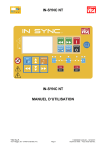
The transition criterions between two states are often one or more logical conditions. Fig. 3.1
displays an example of a state machine. Table 3.1 contain the corresponding transition
criterions for state machine in Fig. 3.1.
13
Fig. 3.1. Example of a state machine.
Table 3.1. Transition conditions for the state machine in Fig. 3.1.
Transition
Name
Condition
T1
ECM initialized
P1X: [WakeUp/KL15)] (HW)
P2X, EUCD: [WakeUp] (HW) or [Kl15] (HW)
T2
T3
Start cranking
Manual Cranking: [StartCrankManuel](INT) i.e [KL 50] (HW) and not
[Startblocking](INT)
Started
Automatic Cranking:
[StartCrankAutomatic] (INT) i.e when cranking conditions are fullfilled,
see ref Error! Reference source not found.
a) ( n > n_start and t > t_start_time)
b) (T > T_start_torque)
Condition a or a+b is Engine and Supplier dependent.
This condition may not be the same condition as when cranking is
stopped,i.e. it is possible to crank when engine is running.
14
T4
Normal stopped
not [KL 15] (HW) and ( n < n_stopped)
Afterrun finished
T6
Stalled
Time, FanReady, Diagnosis Ready, MemStore
Condition is engine and supplier dependent.
n < n_stalled and then set [StalledRecoverReady](INT) (sets for next cycle)
T7
ECM reinitialized
[StalledRecoverReady](INT)
T8
Cranking Deactivated
Manual Cranking: (not [KL 50] (HW) and n=<n_start_crankstoped)
or [Startblocking] (INT) )
T5
Automatic Cranking : not [Cranking](INT) and n<n__start_crankstoped
This condition may not be the same condition as when cranking is
stopped,i.e. it is possible to send engine state cranking when the starter
motor has stoped cranking and the engine is not fully running.
T9
Shutdown
[Afterrun finished](INT)
T10
Shutdown
Not [WakeUp] (HW) and not Started (INT)
In line with Fig. 3.1, a state machine not contains conditions for all possible kinds of
transition. The states not connected with a line are handled as not allowed transitions, under
all circumstances.
3.1.3 Program configuration
The program settings will be done through a Microsoft Excel file (.xls). The Excel file must at
least contain the basic state machine information, i.e. states, allowed transitions and transition
criterions. But the file can also provide classes that run more specific analyzes with
configuration input. Since the program will be constructed in a way that provides good
support and possibilities for future extensions a flexible configuration method is necessary.
3.1.3.1 Basic Analyze configuration
The basic configuration will be a 2-dimensional matrix with the first column and also the first
row containing the state names according to the states of the state machine. It will work as a
jump matrix and covers all possible state transitions. The cells of the matrix constitute either
of a X, which means not allowed transitions under all circumstances, or a T directly followed
by a number (i.e. T2), which means that it follows the transtion condition specified below the
transition matrix as T2 (transition condition 2).
The basic configuration sheet will also contain a table with all transiton conditions, very likely
table 3.1.
In fact the basic configuration is just another representation for a fully configurationally state
machine, like the one in Fig. 3.1.
3.1.3.2 Time Analyze configuration
The program will, as stated above, be provided with the possibility to extend the analyze.
However, it will come with a plug-in module allready with thr program release, namely a
module for analyzing the time in each state. It will be possible to set min-and max time for
each state through a new Excel sheet in the configuration file.
15
3.1.3.3 Signal configuration
In addition to the basic analyze configuration, the Excel file must also contain what
parameters to extract from the log-file, especially how the state parameter corresponds to the
state names in the configuration file.
3.1.4 Verification methods
The verification process will check if the intern state parameter follows the user specifications
in the configuration file. The verification algorithms will cover following sources of error;
•
•
•
•
Not allowed transition
Transition criterions not fullfilled
To short time in state
To limit in state exceeded
In other words, the python program verifies that the state machine implementation works as it
was intended, but not that the implementation itself is correctly specified.
3.2 CAN Interface verification – Theory
3.2.1 Introduction
When connecting nodes, for example different types of control units, with a CAN bus it is of
biggest importance that the node-to-bus interfaces works appropriate. The intern node
parameter must under all conditions have the right coupling to the corresponding extern (CAN
bus) parameter. That means the set of intern parameters must be compared with the
corresponding CAN bus parameters during several types of operation conditions. A mismatch
can cause many types of problems, everything from wrong outdoor temperature in the display
window to a dysfunctional fuel injection.
3.2.2 Theoretical overview
The CAN interface is routing data between the controller unit and Controller Area Network.
The verification strategy is to sample internal controller unit parameter and responding
parameter on the CAN bus, and compare them.
16
3.2.4 Signal processing
Sometimes two parameters with the same behaviour but different gain and/or offset have to be
verified with each other. Therefore functions for scaling and offset have to be implemented.
In some special cases a parameter need to be remapped to fit and be compared by another
parameter. For example, some parameter vectors contain letters that must be remapped to
number values to be processed. A mapping table will be used for that issue.
3.2.5 Verification methods
The main purpose with the can interface will, as mention above, be to compare internal node
parameters with the extern CAN dittos. Therefore some fast, due to the possibility of big
amounts of samples and/or signals, and reliable algorithms for comparing digital vectors is
required.
3.2.5.1 Difference verification
The difference verification just subtracts the two signal vectors element vice. If the difference
in any sample point is to big the verification will fail. How big the difference can be before
the verification fails will be tuneable by the user and also individual for every pair of vectors.
This method is very fast, intuitive and easy to understand, it will hopefully also be good
enough for most signals. Some signal differences may have problems with spikes due to lag
between intern and extern parameters, signal interpolation etcetera, and will therefore be hard
to handle with an algorithm without any type of low pass filtering.
The algorithm contains three, by the user, configurable parameters;
•
•
•
Maximal difference when signal derivative is low
Breakpoint between low and high derivative.
Maximal difference when signal derivative is high
Signal parts with big derivative sometimes require a higher tolerance for differences, due to
badly synchronised signals, and therefore two configuration parameters for signal differences
are needed.
3.2.5.2 Integrated difference verification
The integrated difference verification integrates the difference of the vectors in intervals of
one second each. The maximum allowed value for the integration difference error over a one
second interval will be tuneable by the user and individually for each pair of vectors. This
verification method is more forgivable for short difference spikes than the method described
in 1.5.3.1, but will maybe fail if the difference has a small, but acceptable level, all the time.
In other words; the standard difference verification are searching for peaks and bigger
differences, while the integrated difference verification are searching for small but steady
signal deviations.
The algorithm contains three, by the user, configurable parameters;
•
•
Maximal integrated difference when signal derivative is low
Breakpoint between low and high derivative.
17
•
Maximal integrated difference when signal derivative is high
Signal parts with big derivative sometimes require a higher tolerance for integrated
differences, due to badly synchronised signals, and therefore two configuration parameters for
integrated signal differences are needed.
3.2.5.3 Min/Max verification
Controlling minimum- and maximum values is another verification that has to be done. The
verification will be done after signal processing and therefore only one minimumrespectively one maximum value are required for each pair of signal vectors.
3.2.6 Program configuration
The program configuration will be done in a Microsoft Excel file (.xls). It will contain
possibilities to define what parameters that should be tested, but also the opportunity to adjust
and tune the verification tolerances individually for each pair of parameters.
3.3 Network Management verification – Theory
3.3.1 Introduction
The network management specifies how a CAN node should interrogate and behave during all
possible types of running conditions. A dysfunctional network management can cause serious
problem and it's of great importance to cover all kind of running conditions during the
verification process. For example the node must limp home and use safety settings when the
environment does not work as intended, or enter appropriate after-run states when turned off.
Unfortunately it takes time to run network management test and analyze test logs. To cut the
time for test log analyzing a module for automated network management verification has been
developed
3.3.2 Theoretical Overview
The network management specifies in what modes a node can be running. But also how, and
when, transitions between different modes, or states, are allowed to be done. According to
CAN NETWORK MANAGEMENT 31812308 specification, the states in Table 3.2 can be used
when creating the network management. Remark that the network management
implementation must not contain all states.
Table 3.2. Network management states according to CAN NETWORK MANAGEMENT
31812308
State
Reserved
Off
Start-up
Communication Software init
Operation
Buss Off
Transmission Disconnected
Silent
State numbering
0x00
0x01
0x02
0x03
0x04
0x05
0x06
0x07
18
Wake-up Network
Wake- up pending
Expulsion
Isolated
Expulsion Silent
Expulsion Diagnose
Bus Off Wait / After-run
CAN controller Init / Initialization
Operation After-run
Expulsion After-run
Reserved
Reserved
Stopped
0x08
0x09
0x0A
0x0B
0x0C
0x0D
0x0E
0x0F
0x10
0x11
0x12
0x13
0x14
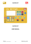
3.3.3 Required states and modes (base flow)
CAN NETWORK MANAGEMENT 31812308 also specify a base flow with required states and
transitions, see Fig. 3.2. The dotted lines are optional transitions. However, remark that the
automated NM verification program will not demand network management based on the
flowing chart in Fig. 3.2 On the other hand it can not contain any other states than in Table
3.2.
15
10
Bus Off
12
Stopped
Bus Off Wait
1
11
16
13
Off
Transmission
Disconnect
14
Software
Download
7
2
6
19
Initialization
4
Operation
5
Expulsion
20
3
17
18
9
Operation
After-run
Expulsion
After-run
Isolated
8
19
Fig. 3.2. Network management base flow according to CAN NETWORK MANAGEMENT
31812308.
3.3.4 Program configuration
The program settings will be done in a Microsoft Excel file (.xls) divided into three sheets,
NMtranistions, powerMode and Signals. The Excel file will be configurable by the user but
with the restriction to follow a template, more information about program configuration can
be found in Appendix B.
3.3.4.1 Main configuration file
The main configuration files will be a 2-dimensional matrix with the first column and also the
first row containing the state names according to specification CAN NETWORK
MANAGEMENT 31812308. It will work as a jump matrix and covers all possible state
transitions. The cells of the matrix constitute of lists with requirements for the state transition,
and will be;
•
•
•
If the jump is allowed to happen.
Other states that have to be entered before the transition are allowed to take place.
Maximum time in state before transition takes place.
In fact the main configuration file's is just another representation for a fully configurationally
flowing chart, like the one in Fig. 3.2 in section 1.5.2, but with additional state transition
criterions.
3.3.4.2 Power mode configuration
The power mode configuration sheet constitutes of lists with allowed power modes for each
state. Power mode can very briefly be described as the electrical status of the car.
3.3.4.3 Signal configuration
The program needs three CAN parameters as input;
•
•
•
Network management state status
Power mode status
Time status
The parameter input configuration sheet provides the python program with names of the
above parameters in the current CAN-log. This feature can't be hard coded since different
nodes use different parameter names.
20
3.3.5 Verification methods
The verification process will check if the network management CAN parameter follows the
user specifications in the main configuration file. The verification algorithms will cover
following sources of error;
•
•
•
Not allowed transition.
Time limit exceeded before state transition.
Not allowed state transition due to not have entered other state or states first.
The verification points above are quite straight on, but maybe the last point needs an
explanation. For example if more than one network management state has to be entered
during the node initialization, the transition criterion for entering the operation mode will be
that all initialization states has been passed through.
4. Program
This chapter is partly about what general program parts are needed for the automated testing,
and partly about purposes, aims and delimitations for each of the different verifications.
The program modules (State machine-, CAN Interface-. and Network Management
verification)) will be created in Python 2.2, and its standard libraries. It will be implemented
in the Power Train Test Automation (PTTA) tool and there constitute the last chain in the test
and verification process. In addition a stand alone user interface will be created for the
opportunity to do verification outside the PTTA environment. With a stand alone GUI it will
be much easier to distribute test versions for debugging and evaluation.
Also Interfaces to flexible generic tools, like Inca, are needed for gathering sufficient program
input.
4.1 General program parts
Some parts of the program is used in all verifications and will therefore be introduced here
and not together with rest of the program description.
4.1.1 Inca as CAN logger
The program Inca, developed by the German company ETAS, will be used for logging the
Controller Area network. Inca can be connected to the CAN-bus or directly to a node through
several different interfaces, depending on sample rate requirements and available contactors.
However the log-file will have the same appearance (disregard sample rates) independent of
the logging method, which of course is an advantage and will make this project easier to
21
handle. What internal node- respectively external CAN-parameters to log can be individually
configured in Inca. A rule of thumb when creating Inca log files for automatic verification is
less is more, since a smaller log file will be faster to process. The log-file will by default be
saved in .dat format. When recreating the measurement in MDA, which is ETAS signal
analyzing tool, the .dat-file is interpreted by a database. In this way the log-file becomes quite
small, but for our purpose it's better to export the .dat-file to an ASCII-file (.txt), since Python
contains powerful tools for processing text files.
The log file generated by Inca need some processing before it can be used in the verification
algorithms. First of all Inca samples the time vector faster than the measurements are
sampled, the measurement vectors contains therefore a lot of empty sample points that have to
be handled before any mathematical processing can be done. The best, and simplest, way is to
interpolate the missing sample points. For this project a first order hold algorithm (linear
interpolation) will probably be the best compromise between precision and calculation
capacity. The empty sample points before the first measurement will be deleted.
4.1.2 Program configuration
The program serttings will be done in a Microsoft Excel file. The configuration file will not
have the same appearance for every verifiaction method. The configuration file is the only
program flexibility there is. The file is parsed into the program through Microsoft Windows
COM Interface.
4.1.3 Result presentation
A result file is created after a successful verification process. The file is in “.xls” format and
created through Microsoft Windows COM Interface. First of all the file contains the
verification result, but also useful additional information for allocating errors and bugs. The
result presentation are not equal for the different kinds of verification methods.
4.2 State Machine program
4.2.1 Background
The state machines are today verified by manually change and manipulate (inject errors etc.)
the environment, and either in real time or via a log file assess if the states are correct in
respect to the current environment. Both the real time view and logging functionality is
managed by a program called Inca. It's possible to log both node (intern) parameters and
CAN-bus parameters. An Inca log-file can be saved in either a '.dat' format for process and
analyze in MDA (an analyze tool for Inca log-files) or in ASCII format for analyze in a text
editor.
The setup for a state machine verification can be either a development car or a computer
based simulation environment, with possibility to read node parameters.
22
4.2.2 Purpose and aims
The manually state machine verification takes time, and the demanded time for verification
will incease along with upscaling of the cars electronic network. Verification of growing
electronic networks can be handled in at least three different ways;
* Recruite more people in the same speed as the working load increase.
* Cut down the time for each verification process to handle the increased working load.
* Evolve and make the verification processes more efficient.
The aim is to create a reliable automatic state machine verification tool with purpose to
considerale decrease the time demanded for state machine verification. The task will be done
by developing a log-file processing tool in the language python. The final goal is a proper and
well working implementation of the verification tool in the simulation environment used on
VCC.
4.2.3 Delimitations
The aim is to build a very dynamic and adaptable Python class library. But there will of
course be delimitations that the user most have knowledge about. The most important
delimitations are shown above.
•
•
All node parameters that are used by the state machine most be able to log.
The program scripts can only verify logical expressions of parameters with same time
stamp, i.e. logical expressions with not synchronized parameters can't be handled.
However, it's in most cases possible to handle this types of limitations by expand the basic
class library with a new class, tailor made for the current task.
4.3 CAN interface program
4.3.1 Background
The can interface is verified today by manual studying of the parameter behavior during
different types of operations and condition settings, either in real time or via a log file. Volvo
car Corporation uses Inca among others for logging the CAN and node activities. The
program provides the user with possibilities to choose what signals to analyze, sample rate,
scaling, offset etcetera. The log file can be saved either in ETAS own format '.dat' or in a
common ASCII ('.txt') representation.
4.3.2 Purpose and aims
Manually analyzing the CAN interface is very time demanding today, and will be even worse
in the future along with more complex CAN network layouts. The aim will be to create a
reliable automatic verification model with the purpose to considerable decrease the time
demanded for CAN interface verification. The task will be done by implementing a new
function library in the scripting language Python, which are able to handle and analyze ASCII
log files from Inca. Another aim is, after a successful development, use the CAN interface
library in a simulation environment which automatically will generate an Inca log file for the
chosen simulator settings.
23
4.3.3 Delimitations
It will hopefully be few delimitations when the function library are finished. The Python
scripts will be close, but never able to cover every possible kind of CAN parameter
verification. One of the main reason is to hold down the complexity of the, from user,
demanded configurations and settings. Another problem that may occur is slow performance
and allocation of all available RAM when using big log files (e.g. many samples and/or
parameters) in combination with many parameters for verification.
4.4 Network Management program
4.4.1 Background
The network management is verified today by manually studying the behavior during
different types of operations and condition settings, either in real time or via a log file. Volvo
Car Corporation uses Inca among others for logging the CAN and node activities. The
program provides the user with possibilities to choose what signals to analyze, sample rate,
scaling and offset. The log file can be saved either in Inca’s own format '.dat' or in a common
ASCII ('.txt') representation.
4.4.2 Purpose and aims
As mention in the introduction part the time effort for testing network management manually
are in many cases huge. The aim will be to create a reliable automatic verification model with
the purpose to considerable decrease the time demanded for the verification process. The task
will be done by implementing a new function library, in the scripting language Python, which
is able to handle and analyze ASCII log files from Inca. Another aim is, after a successful
development, use the network management library in a simulation environment which
automatically will generate an Inca log file for the chosen simulator settings.
4.4.3 Delimitations
The program will hopefully be quite flexible, but with at least one big restriction. The node
must under all circumstances follow the specifications in CAN NETWORK MANAGEMENT
31812308. It is the official specification for network management in, among others, the
Engine Controller Module and Transmission Controller Module.
Another problem that may occur is slow performance when using large log files (e.g. many
samples and/or parameters).
24
5. Result
The finished verification programs are described, how it is constructed both in an overview
perspective but also on detail level, in this chapter. There are also examples of verification
results.
5.1 Result, State Machine Verification
5.1.1 Result overview
The state machine verification program contains following parts;
•
•
•
Python module OMM_LIB.py.
Template for configuration file
Result presentation in form of automatically generated Excel files.
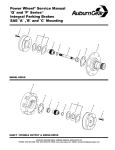
Fig. 5.1 is an overview of the program structure represented as an UML class chart.
According to the class chart, the program contains classes for handling of input, result and
analyzes. But also a control class that instantiate the other classes and execute class functions.
It is possible to pick and choose what type of analyze classes to use for the verification. It is
also possible to create own analyze classes for inceased flexibility. Fig. 5.2 is a simplified
overview of the program execution order, represented in UML format.
Fig. 5.1. UML class chart diagram for state machine verification program.
25
Fig. 5.2. State flow for state machine verification program.
5.1.2 Program module OMM_LIB.py
The program module OMM_LIB.py contain all code for verification of state machines. The
code is splitted into four categories;
•
•
•
•
Input handling
Exit handling
Controller
Analyze/verification handling
See Fig. 5.1 for the UML description.
5.1.2.1 Class InputHandler
The class InputHandler contain functionality to process and extract data from an Inca log-file.
Table 5.1 describes the functions of InputHandler.
Table 5.1. Function declaration for class InputHandler.
Function
getMeasurement
getSignalsMatrix
openConfigWorkbook
Description
Extracts the information from an Inca log-file and save the raw data in a local
variable.
Process the raw data (interpolate empty samples etc.) and extracts parameter
vectors according to the configuration file, and save it as a 2-dimensional matrix.
Sets up all connections with the Excel application and open the configuration file.
5.1.2.2 Class ExitHandler
The class ExitHandler saves the result and closes the used applications, i.e Microsoft Excel.
Does not contain any callable functions, everything is done when the class is instantiated.
5.1.2.3 Class OMManalyzer
The class OMManalyzer is the program controller. It instantiate the other classes and handles
the function calls. OMManalyzer doesn't contain any functions itself, which means the
verification process starts when the class is initialized and in the end produce a result file
without any other lines of code. The OMManalyzer needs 4 arguments.
•
•
Address to the Inca log-file.
Address to the Excel configuration file.
26
•
•
Address to the result destination.
A list of names on what types of analyzes to instantiate and run.
OMManalyzer will automatically instantiate InputHandler, ExitHandler and the chosen
analyzes. It also does the necessary function calls for each initialized class.
5.1.2.4 Analyze classes
The analyze classes are responsible for verification result. In other words is the choice of
analyze classes, for a certain analyze, that decides the verification focus. For example, if the
time in each state is the only thing of interest for a certain verification, just instantiate the time
analyze class and skip the other analyze types then. There are also good possibilities to extend
the class library with new types of analyzes. The existing analyze types are created after a
generic implementation method, and as long as the new analyze class follow this method it
will be recognized and handled in a correct way by the OMManalyzer class. A analyze class
must contain the functions described in Table 5.2.
Table 5.2. Function declaration for the Analyze classes.
Function
getConfiguration
startAnalyze
resultHandler
Description
Gets the necessary information from the configuration file.
Starts the analyze of the chosen parameter vectors extracted from the Inca logfile.
Organizes the result from the analyze and writes it to a new excel sheet.
5.1.2.5 Configuration file
The Excel configuration file must at least contain two sheets, one with information what
signals to extract and process from the log-file and another with the state machine
architecture. Fig. 5.3 and Fig. 5.4 display how the above mentioned Excel sheets can look
like.
27
Fig. 5.3. Example of how the state machine architecture is constructed in the configuration
file.
Fig. 5.4. Example of signal configuration to the left. How the state parameter will be parsed is
configured on the right hand side.
Note that the logical transition conditions in Fig. 5.3 follows python (and most other
programming languages as well) notation. For example implies the sign "=" assignment and
"==" equal to. The following operators can be used;
•
•
•
•
•
•
•
•
==
<
>
<=
>=
and
or
not
Also remark that the parameters fetched from the Inca log-file is renamed to shorters and
more intuitive names (for example names used in the specification from the controller system
supplier).
28
In addition to the two sheets mentioned above, the configuration file can include more sheets
with configurations for other analyzes. Fig. 5.5 displays how the configurations for the time
analyze can look like. The times in each states are specified in seconds (-1 means no
limitations).
Fig. 5.5. Example of a time analyze configuration.
5.1.3 Result presentation
A successful State machine analyze generates an Excel result log. All state transition and
belonging information is notated in the result log. The number of sheets varies and depends
on which and how many analyzes was processed. The following figures, Fig. 5.6 and Fig. 5.7,
are examples of the result log.
29
Fig. 5.6. Basic Analyze result log.
Fig. 5.7. Time Analyze result log.
The analyze results are colour coded, where green implies that everything is ok, red colour
implies that something is wrong. Fig. 6 contain two red marked transition, transition 1 and
transition 4. Transition 1 fails because the configuration file (sheet signal configuration) not
contains information of how to parse the state parameter value "0". Transition 4 fails because
30
unfulfilled transition condition. The transition condition is "KL 15 == 1", but as seen in Fig.
5.6 the current value for "KL 15" is "0.0". Both this are deliberately injected errors, the
configuration file in 1.6.3 would not give such error. The red marked fields in the time
analyze result log (Fig. 5.7) either mean that the state wasn't found in the time analyze
configuration or the time in state is below the min time or exceeds the max time.
Some project requires tailor made analyzes for one single purpose. Fig. 5.8 displays the result
log of such tailor made analyze for I5D engineState (state machine in the engine controller
system of a Volvo diesel). The only purpose for this analyze class is searching for the
transition "COENG_RUNNING Æ COENG_READY" and verify the transition condition if
found. The transition condition includes time requirements for some parameters and is
therefore too complicated for the basic analyze to handle.
Fig. 5.8. Result log for I5D engineState tailor made analyze.
5.1.4 Discussion
5.1.4.1 Program functionality
The program works, as far at it has been tested, as intended. And the implementation runs in
the way it was specified. The class library that exists today will probably not cover all types
of future state machine verifications, but the program controller is well prepared for
implementation of new analyze-classes.
It takes some time to be familiar with the program user interface, but is anyway probably
constructed in simplest possible way. A flexible program with big configuration possibility
always demand some time effort of the user before it become a strong and time saving tool.
5.1.4.2 Known problems and bugs
No bugs or problems detected. But new types of state machines will most likely require
additional, new developed, analyze classes. But it's more a limitation rather than a problem.
The program needs a better evaluation before confirming that it is free from bugs.
5.1.5 Conclusion
The state machine verification program works very well. It is fast, flexible and in this
connection easy to use. A lot of responsibility is given to the user. A configuration miss can
31
cause verification errors, or even worse; not detecting state machine bugs and errors. But
that's the price to pay for flexible solutions.
Developing of new analyze classes will probably be required for a total verification future
state machines.
5.1.6 Future work
•
Developing new analyze classes to meet up with the verification requirements of
upcoming state machines.
•
Create configuration files for more state machines.
•
Improve GUI to simplify for the user.
32
5.2 Result, CAN Interface Verification
5.2.1 Result overview
The finished CAN interface verification program contains following parts;
•
•
•
•
•
Python library CANinterface_LIB.py.
Configuration file, for example CANconfiguration.xls.
Mapping tables, for example mapping1 sheet in CANconfiguration.xls.
Stand alone user interface GUI.py.
Result file, for example result.xls.
The program starts with reading the CAN log and configuration file. It will then start to fetch
pairs of parameter names to compare from the configuration file. The parameters
corresponding measurement vectors are fetched from the CAN log, and the signal- and
verification processes starts. The result is stored in a program variable. This procedure repeats
until all parameters are fetched from the configuration file, and the result is written to the
result log. See Fig. 5.9 for an overview of the program execution order.
Fig 5.9. UML state chart diagram of the verification program.
5.2.2 Program module
The program library CANinterface_LIB.py contains all functions that are callable through
PTTA or the stand alone GUI. A functions declaration can be found in Table 5.3.
Table 5.3. Function declaration for CANinterface_LIB.py.
Function
readFromFile
readSettingsFromExcel
findCanColumn
getColumnLin
syncParam
uTest
executeConfig
resultToExcelWriter
Description
Reads the CAN file
Reads the excel configuration file.
Finds the right CAN file column due to the required parameters in the configuration
file
Extract a column in the CAN file due to the parameters in the configuration file.
Uses a first order hold algorithm to interpolate empty samples.
Sync two measurement vectors.
Contains the CAN interface testing algorithm
Executes the CAN interface verification
Write the CAN interface verification result to a Microsoft Excel file (.xls) through
the COM interface
5.2.2 Configuration file
The appearance of the configuration file is more or most hard coded and very few deviations
will be accepted. For an example of a correct configuration file, see Fig. 5.10. Note that
comments only can be done in the first column and must be proceeding by double number
33
signs (##). Also remark that links to mapping files can't contain single backslashes due to
Python notation. All single backslashes must therefore be replaced by either a single
frontslash or double backslashes.
Fig. 5.10. Example of a correct CAN interface configuration file.
3.2.6.4 Mapping tables
The mapping tables constitutes of a simple Excel-sheet. The mapping tables are used for
mapping one or more values to other values. For example, this functionality is needed if the
internal parameter who sample the gear selector use the values [p, r, n, d] and the CAN dito
uses the numbers [0, 1, 2, 3] instead. Fig. 5.11 and 5.12 are examples of how a mapping table
looks like.
Mapping2
Mapping1
From
2.0
3.0
4.0
From
To
150
2700
3000
Fig. 5.11. Mapping table Example.
To
p
r
n
d
0
1
2
3
Fig.
5.12.
Another
mapping table example.
5.2.3 Stand alone user interface
See Appendix A for a brief description of the simple stand alone user interface.
5.2.4 Logging result
5.2.4.1 Result file
A successful CAN interface analysis generates a result log. The result file contains
information of both the settings and result. The first table is a copy of the configuration file
and the second table contains the verification results.
34
Fig. 5.13. CAN interface verification results for a Jaguar car.
The result file contains three more sheets in addition to the result sheet;
•
•
•
Integrated difference (diffintegration) errors.
Difference errors.
MinMax errors.
The additional sheets contain detailed verification logs. Fig. 5.14 shows an example of a
difference errors log.
35
Fig. 5.14. Part of a difference errors log.
5.2.4.2 Plots
In addition to the result log, plots are also automatically generated for signals that didn't pass
the verification processes. Plots are a very good complementary to the result file when it's
hard to decide if the verification shall pass or fail. See Fig. 5.15 for an example.
36
Fig. 5.15. Example of two signals that didn't pass the verification processes. It's not hard to
understand why it failed.
5.2.5 Discussion
5.2.5.1 Program functionality
The program works, as far at it has been tested, as intended. The implementation runs in the
way it was specified. It takes some time to be comfortable with the program and its
mechanics, the demanded user inputs are quite big. The main focus during development was
flexibility rather then user simplicity. The program will exclusively be used by an analyze and
verification group at Volvo car company, who required a program for handling more or most
all the CAN interface verification. The need of a simple to use program for everyone was
therefore non-existent.
5.2.5.2 Known problems and bugs
There are, at least, two major problems with automated CAN interface verification;
•
•
Handling big Inca measurement logs in combination with many verification
parameters may allocate all RAM.
Verify pair of parameters which are asynchronous in time and contain big variations
with rapid changing.
Big measurement logs (≈100Mb and above) in combination with many verification
parameters mean a lot of sample points to read and process, which takes time for the Python
interpreter to process. It can also result in allocation of all free RAM, which will decrease the
37
system performance a lot. Unfortunately the automated, and in most cases very comfortable,
memory allocation in Python doesn't handle this problem in the best of ways. Python is fast
for being an interpreting language, but not comparable with compiled languages such as C. In
addition, in C all memory allocation is controlled by the programmer. Maybe the Python code
can be optimized due to execution time in some points, but will then be much harder-to-grasp
and edited.
Comparing two parameters with bad time synchronisation and rapid changing will lead to big
difference errors and even sometimes a fair difference integration error. It means the user
must be aware of the approximate look and behaviour of the tested parameters when tuning
the allowed error levels. A more sophisticated signal processing would probably partly handle
this problem, but on the other side lead to a longer execution time. This is over all a minor
problem, and a very few parameters are affected, compared to increase the execution time
further.
The program is designed to run on a windows platform with office 2003 installed. It seems
like the interface to win32 COM in office 2007 slightly differs from the 2003 version in some
points. Hopefully (and as far It's tested) it' will work as intended also on a platform with office
2007.
5.2.6 Conclusion
More or most all types of CAN interface parameters can be verified with this program
module. But the user must be aware of how to configure it for every single parameter pair to
get a useful result. That will however presumably not be a problem; it will exclusively be
configured and used by experienced CAN verifiers.
The functionality and performance will be best when using moderately big log files (≈5-50
Mb), and the crashing risk will be minimal.
5.2.7 Future work
•
•
•
Writing big parts of the module in a compiling language, preferable C, will speed up
the execution time a bit. However the program runs today sufficiently fast for the most
applications.
Extend the program flexibility and possibility to cover even more, or maybe future,
types of CAN parameters. The seamy side with extended flexibility will be a more
unwieldy configuration file.
Refine and optimize the code for faster execution and readability. Not a big need, but
refining can always be done until end of days though.
38
5.3 Result, Network Management
5.3.1 Result overview
The finished Network Management verification program contains following parts;
•
•
•
•
•
•
Python module NM_LIB.py.
NMtransition configuration, as sheet in for example NMconfiguration.xls.
Signals configuration, as sheet in for example NMconfiguration.xls.
Power mode settings, as sheet in for example NMconfiguration.xls.
Stand alone user interface GUI.py.
Result file, for example result.xls.
Fig. 5.16 is a shortly description of the program functionality represented in an UML state
chart diagram. According to state chart diagram the program starts with reading the Network
management log and configuration file. It will then fetch the needed parameter (or signal)
vectors from the CAN-log.
Fig. 5.16. UML state chart diagram of the Network Management verification program.
5.3.2 Program module
The program module NM_LIB.py contains all functions that are callable through PTTA or the
stand alone GUI. The function declaration can be found in Table 5.4.
Table 5.4. Function declaration for NM_LIB.py.
Function
CanFileReader
allInOneMatrixReader
conditionMatrixReader
pmReader
findCanColumn
getPointedCanVector
getPointedCanMatrix
pCanMatrixVerification
getStateInTime
getLastValue
appendLog
Description
Reads the CAN file
Reads the first (NMtransition) sheet in the configuration file
Reads the Signal sheet in configuration file
Reads the power mode sheet in configuration file
Finds the right CAN file column due to the required parameters in the parameter
file.
Extract a column in the CAN file due to the parameters in the parameter file. Uses
a zero order hold algorithm to interpolate empty samples.
Merges the extracted columns from getPointedCanVector.
Verifying the network management
Extract the network management state for a given
Extract the last network management state in the Can log
Adds a text string to the result file
39
5.3.3 Configurations
5.3.3.1 Main configuration sheet
The NMtransition sheet is, as mentioned in 1.5.4.1, a documentation of criterions for all
possible transitions. The left most column contains the from states, while the first row
contains the to state. See Fig. 5.17 for an example. Note that the cells are unexpanded.
In addition to the transition matrix it also contains a table for activation or deactivation of
tests. A test is searching for a specific combination of transitions, specified in the
configuration file in the sheet with the same name as the test. For example; configurations for
the test Bus off can be found in the sheet named Bus off.
Fig. 5.17. Network management main configuration sheet.
Fig. 5.18. Part of NM configuration file. NM state transition criterions from Operation to Off
are red marked.
The state transition criterion can either contain the character x or a string of the same type as
in Fig. 5.18. If the transition criterion between two states is x marked means the transition
can't be done. It can for example be from or to a non used state in a specific implementation.
In Fig. 5.17 the transition from or to the Start-up state are marked with an x because that NM
40
state isn't used in the example implementation, the same goes for Reserved and a number of
other NM states.
If the transition criterion contains a text string, like the red marked one in Fig. 5.18, the
analysis will use that string as input. The text string contents with descriptions are listed in
Table 5.5. In fact the text strings follows the Python notation and are therefore ideally as
program input.
Table 5.5. NM state transition criterions
Variabel name
AJ
JC
JT
Description
Stands for Allowed Jump.
Equal to 1 means allowed transition
Equal to 0 means not allowed transition
Stands for Jump Criterions.
Contains a list with states which must have been entered before transition. If no
criterions, the list will only contain the single value -1.
Stands for Jump Time.
Contains the maximum time for the transition to be done
5.3.3.2 Power mode settings
The power mode settings are done in the PoweMode sheet of the configuration file. It contains
the allowed power modes for each network management state. Fig. 5.19 is an example for
how the setting file should look like.
NM PM Settings
State
Allowed powermode
Reserved
Off
Start-up
Communication Software Init
Operation
Bus Off
Transmission Disconnect
Silent
Wake-up Network
Wake-up Pending
Expulsion
Isolated
Expulsion Silent
Expulsion Diagnose
Bus Off Wait/After-run
Can Controller Init/Initialization
Operation After-run
Expulsion After-run
Reserved
Reserved
Stopped
PM=[2,3,4,5,6]
PM=[2,3,4,5,6]
PM=[2,3,4,5,6]
PM=[2,3,4,5,6]
PM=[2,3,4,5,6,7]
PM=[2,3,4,5,6]
PM=[2,3,4,5,6]
PM=[2,3,4,5,6]
PM=[2,3,4,5,6]
PM=[2,3,4,5,6]
PM=[2,3,4,5,6]
PM=[2,3,4,5,6]
PM=[2,3,4,5,6]
PM=[2,3,4,5,6]
PM=[2,3,4,5,6]
PM=[2,3,4,5,6]
PM=[2,3,4,5,6]
PM=[2,3,4,5,6]
PM=[2,3,4,5,6]
PM=[2,3,4,5,6]
PM=[2,3,4,5,6]
Fig. 5.19. Example of a Power mode settings file.
41
5.3.3.3 Signal settings
Also the parameter settings are configured via the Excel Sheet Sginals. The left column
contain the python program parameter name, while the right column contains the respective
CAN-log address. See Fig. 5.20 for an example.
NM signal Settings
Type of parameter
Parameter name
Time
NM state
PM keyPos or likely
time
diag_NW_States\CCP:1
PowerMode
Fig. 5.20. Example of a signal settings file.
5.3.3.4 Settings for special tests
As mentioned in 1.6.3.1, there are a number of special tests. Each of these tests has its own
configuration sheet, see Fig. 5.21 for an example. The special test configurations contain a
three column table. The first column specifies what combination of states to search for. The
other two columns specifies min- and max-time in each state.
Fig. 5.21. Bus off test configurations.
5.3.3.5 Stand alone user interface
See Appendix B for a brief description of the simple stand alone user interface.
5.3.4 Result File
A successful Network Management analysis generates a Microsoft Excel result file. All
upcoming network management errors during the verification are presented in the result file.
In addition, the last part of the log contains results for the activated special tests. See Fig. 5.22
for an example log.
42
Fig. 5.22. Example of a Network Management result file.
5.3.4.1 General NM errors
The first part of the result file presents all general Network Management errors. It can be all
from an illicit transition to wrong powermode or unidentified states. In addition, all passed
states are presented in the order they were activated.
5.3.4.2 Specific NM verification
The log file's second and last part contains the result of the special tests. Each match of the
specified state series is presented. Whole or part of the series can either be marked as ok in
green colour, or as failed in red colour. Failed means time in state whether is below the
minimum time limit or exceeds the maximum time limit.
5.3.5 Discussion
5.3.5.1 Program functionality
The program works as intended, as far at it has been tested. The implementation runs in the
way it was specified. The by far biggest risk when using the program is wrong configurations
(set by the user) according to specification. But the program will exclusively be used by an
analyze and verification group at Volvo car company and flexibility was therefore prioritized,
instead of use ability.
It takes some time to be comfortable with the program and its mechanics, the demanded user
inputs are quite big. The main focus during development was flexibility rather then user
43
simplicity, and a program that can handle more or most all the Network Management
verification. The need of a simple to use program that everyone can use for verifying the
Network Management was therefore non-existent.
5.3.5.2 Known problems and bugs
There are no recognized bugs, as far as tested.
5.3.6 Conclusion
The program can be used for verifying the Network Management in most cases. The seamy
side is an ungainly configuration file. The configuration file design can be improved in a
plural ways. Not much job is done there though, because the state machine verification
algorithms can in most cases be used also for verifying the Network Management state
machine.
5.3.7 Future work
•
Cleaner code and user interface are needed, specially the configuration interface needs
an update.
•
Update the state machine verification code to fully include also network management.
This software will then be replaced with the state machine verification tool, which is
much more flexible.
44
6. Discussion and Conclusion
Profits and disadvantages for automated verification in general are discussed in this chapter.
Especially time profits and useability for automated verification methods are highlighted.
6.1. Program functionality and useability
The overall program functionality, and particularly the usability, for PowerTrain Test
Automation (PTTA) is now, with the log-file verification and result presenting implemented,
improved. And the step from development- to commercial software has significantly
decreased.
The PTTA system itself is a very flexible tool with big opportunities. The program parts
developed, scripted and tested in this thesis are developed in the same spirit, and will
hopefully be flexible enough to analyze and verify also future State machines, Network
management and CAN interface architectures. But software tools with high flexibility, as
everything else, also has a seamy side; the demand of competence and experienced manpower
for handling the program configuration. To learn and master PTTA is sadly not the only
obstacle. It also requires adaptation of a whole test environment, namely the car, to a
simulated ditto. That requires of course great efforts from the developers of the simulator and
its surrounding environment to get things work in a proper way, but also from the users. They
have to change, or in many cases try new, ways of working.
This thesis has only been about verification of three different types of controller unit
functions, and it maybe seems like verify these collection of functions in a manual or
automatic way doesn't matter. But that's wrong, at least from two very important perspectives.
First; these three are somewhat the absolutely most time consuming functions to verify,
especially the CAN-interface. And the verification has to, or at least should, be done with
every new software update. Second; hopefully this thesis in combination with the other parts
of PTTA works as a good example and guidance for future work.
6.2. Time profits
The time savings for using automatic verification methods instead of manual must be
managed as the very most important parameter during the whole development process. It's,
without question, the heaviest argument when convincing the possible user to change working
methods. Other important parameters are of course reliability, storage functions, flexibility
etc, but not nearly as important, for the user, as the time profits.
The configuration and first run for a whole new controller unit, independent of it's verification
of CAN-interface, network management or the engine state machine, will take about the same
time as to test it manually. In other words; it will take 4 hours or more, dependent of software,
type of function for verification, coverage etc. The big time profits are instead received when
iterating the verification process, for example when a new software update is released.
Usually a controller unit last for 3-6 years. That implies plenty of software updates; in general
40-50 updates a year. With that basis just a single hour time profit when using automatic
verification methods is a huge time save.
45
6.3. Problems and pitfalls
There are of course, apart from the benefits, also several problems and pitfalls with using
automated verifications. The biggest source of error for manual verification is without doubt
the human factor. But I will say the same goes for automatic verification if the algorithms
itself is verified in a proper way. It can be everything from incorrect configuration to wrong
result interpretation. But of course, the tester must be aware of program flaws, even if it's well
tested. One of the most important qualities for the tester to possess is the capacity for estimate
the reliability of the result, just because it's so easy to inject an error in the configuration.
6.4. The importance of satisfying specifications
A prerequisite for automatic verification of controller unit functions is good and exhaustive
specifications. Of course good function specifications are also required if the verification is
done manually, but it doesn't have to be crystal clear in every single way. A manual test is
allways, and will allways be, much more flexible than automatic tests. If something are not
clear or not mentioned in the specification of the function the manual tester, in many cases,
can decide if the function is ok just by using his/her logical mind and experience. The
function will of course not follow the specification to hundred percent, but it's at least
working. That flexibility will never be reached by using automatic tests. An automatic
verification algorithm contains as much intelligence, neither more or less, as required for
verifying that the implementation follows specification. In the very most cases a bad function
specification leads to bad or useless automatic test results.
7. Future Work
The future work in the automated software verification area is endless. This thesis, combined
with the PTTA development, is just a first step in the right direction and guidance for future
strategies. But if we just focus on future work strongly connected to this thesis, the following
points are important to handle in the near future;
•
•
Extend the library of configuration files for verification of more types of controller
unit software. The automated test system is designed to work with all available TCM
and ECM software, but it's only tested with a few ones because the lack of
configuration files.
Education of the testers in the new way of work. Automated testing requires in many
cases both different kind of competence and work approach than manual testing.
46
8. Bibliography
[1]
M. Lutz, Programming Python, O'Reilly Media, Inc, 1996
[2]
CAN specification version 2.0, Robert Bosch GmbH, 1991
[3]
Steve Corrigan, Introduction to the Controller Area Network (CAN),
Texas Instruments Incorporated, 2003
[4]
Runar Frimansson, Personal Communication, September-December
2008.
[5]
Niklas Smith, Personal Communication, September-December 2008.
47
Appendix 1
1. State machine verification – user manual
1.1 Introduction
The program is written in the interpreting language Python and is used for verification of state
machines. See Fig.1 for an example of a state machine. The intention is to change from
manually state machine verification to scripted algorithms and analysis tools. The program
requires an Inca measurement log-file as input. Remark that the file must be saved in ASCII
(.dxl) format. The verification program contain following parts;
•
•
•
Python module OMM_LIB.py.
Template for configuration file
Result presentation in form of automatically generated Excel files.
Fig.1. Example of a state machine.
1.2 Program module OMM_LIB.py
1.2.1 Overview
The library, OMM_LIB.py, contains classes for input/output-handling, signal processing and
verification. See Fig. 2 for an overview of the program execution order. It is possible to
48
choose what types and how many analyzes to use for the current state machine verification. It
is also possible to connect new analyze classes to the verification tool, if the existing ones
doesn't fit the current purpose.
Fig. 2. State flow for state machine verification program.
1.3 Analyze classes
The analyze classes are responsible for verification result. In other words is the choice of
analyze classes, for a certain analyze, that decides the focus of the verification. For example,
if the time in each state is the only thing of interest for a certain verification, just instantiate
the time analyze class and skip the other analyze types then. There are also good possibilities
to extend the class library with new types of analyzes. The existing analyze types are created
after a generic implementation method, and as long as the new analyze class follow this
method it will be recognized and handled in a correct way by the verification tool. A analyze
class must contain the functions described in Table 3.
Table 1. Function declaration for the Analyze classes.
Function
getConfiguration
startAnalyze
resultHandler
Description
Gets the necessary information from the configuration file.
Starts the analyze of the chosen parameter vectors extracted from the Inca logfile.
Organizes the result from the analyze and writes it to a new excel sheet.
Currently there are three created analyze classes;
•
•
•
Basic Analyze
Time Analyze
Special Analyze for I5D-engineState.
The basic and- time analyze classes are general algorithms for state machine verification,
while the special analyze is tailor made for I5D-engineState verification.
1.3.1 Basic Analyze
The basic analyze search for eligible state transitions in the log-file, in respect to transition
conditions. Many state transitions are never allowed (i.e. the one not connected with an arrow
in Fig. 1). Errors will be presented in the result file.
1.3.2 Time Analyze
Calculates and verifies the time in each state. Errors will be presented in the result file.
49
1.4 Configuration file
The Excel configuration file must at least contain two sheets, one with information what
signals to extract and process from the log-file and another with the state machine
architecture. Fig. 3 and Fig. 4 display how the mentioned Excel sheets can look like.
Fig. 3. Example of how the state machine architecture is constructed in the configuration file.
Fig. 4. Example of signal configuration to the left. How the state parameter will be parsed is
configured on the right hand side.
Note that the logical transition conditions in Fig.3 follows python (and most other
programming languages as well) notation. For example implies the sign "=" assignment and
"==" equal to. The following operators can be used;
•
•
•
•
•
•
==
<
>
<=
>=
!=
50
•
•
•
and
or
not
Also remark that the parameters fetched from the Inca log-file is renamed to shorter and more
intuitive names (for example names used in the specification from the controller system
supplier).
In addition to the two sheets mentioned above, the configuration file can include more sheets
with configurations for other analyzes. Fig. 5 displays how the configurations for the time
analyze can look like.
Fig. 5. Example of a time analyze configuration.
1.5 Result presentation
A successful State machine analyze generates an Excel result log. All state transition and
belonging information is notated in the result log. The number of sheets varies and depends
on which and how many analyzes was processed. The following figures, Fig. 6 and Fig. 7, are
examples of the result log.
51
Fig. 6. Basic Analyze result log.
Fig. 7. Time Analyze result log.
The analyze results are colour coded, where green implies that everything is ok, red colour
implies that something is wrong. Fig. 6 contain two red marked transition, transition 1 and
transition 4. Transition 1 fails because the configuration file (sheet signal configuration) not
contains information of how to parse the state parameter value "0". Transition 4 fails because
unfulfilled transition condition. The transition condition is "KL 15 == 1", but as seen in Fig.6
52
the current value for "KL 15" is "0.0". Both this are deliberately injected errors, the
configuration file in 1.6.3 would not give such error. The red marked fields in the time
analyze result log (Fig.7) either mean that the state wasn't found in the time analyze
configuration or the time in state is below the min time or exceeds the max time.
1.6 User Interface
This verification tool will be implemented in the power train test automation (PTTA) program
and its graphical user interface. PTTA is a tool for automatically generate and verify log-files
for different operation conditions, decided by the user. In other words; it takes care of the
whole chain, from simulator configuration to log generation and verification.
53
2. CAN interface verification – user manual
2.1 Program overview
The program is written in the interpreting language Python and used for CAN interface
verification. The intention is to change from manually CAN interface verification to scripted
algorithms and analysis tools. The program needs an Inca measurement log as input. Remark
that the file must be saved in ASCII (.dxl) format. This analysis tool can be used for both
TCM and ECM CAN interface verification. Fig.1 is a brief overview of the program's
execution order. The program itself contains the following parts:
•
•
•
•
•
Python module CANinterface_LIB.py
Configuration file, for example CANconfiguration.txt
Mapping tables, for example mapping1 sheet
Stand alone user interface GUI.py.
Result file, for example result.xls
Fig 1. UML flowing chart for the CAN interface verification algorithm.
2.2 Delimitations
It will hopefully be few delimitations, but there will always be test settings of non standard
type the program can't handle. The main reason not cover every possible test case is to hold
down the complexity in the, from user, demanded configurations and settings. It will neither
be time sufficient implement everything. Another problem that may occur is slow
performance and allocation of all available RAM when using big log files (e.g. many samples
and/or parameters) in combination with many verification parameters.
54
2.3 CANinterface_LIB module
CANinterface_LIB.py is the home for all implemented functions that are callable through the
user interface. Table 1 shows the containing functions.
Table 1. Function declaration for CANinterface_LIB.py.
Function
readFromFile
readSettingsFromExcel
findCanColumn
getColumnLin
syncParam
uTest
executeConfig
resultToExcelWriter
Description
Reads the CAN file
Reads the configuration file through COM interface
Finds the right CAN file column due to the required parameters in the configuration
file
Extract a column in the CAN file due to the parameters in the configuration file.
Uses a first order hold algorithm to interpolate empty samples.
Sync two measurement vectors.
Contains the CAN interface testing algorithm
Executes the CAN interface verification
Write the CAN interface verification result to a Microsoft Excel file (.xls) through
the COM interface
2.4 Configuration file
The CAN interface configuration file must be an Excel file (.xls) and contain one or more
sheets. For a configuration file example, see Fig. 2. The file provides the program with user
defined test settings such as processing parameters and tolerances.
Fig. 2. CAN interface configuration file.
2.4.1 Parameters
The first two columns in the CAN configuration file contain the test parameters. Parameter1 is
tested against the contiguous Parameter2. It's advisable to let the parameter names in the
configuration file be exactly the same as in the Inca CAN log to avoid problems. If the
55
parameter's corresponding value vector contains literals they have to be mapped, please read
section 2.2.7.
2.4.2 Scaling
The third column in the CAN configuration file contains information of how Parameter2 will
be scaled. The scaling algorithm is very simple, Parameter2 is just multiplied with the scaling
value. For example; if the scaling value is 3 Parameter2 will be three times as big as the
original. Scaling value one means no scaling at all.
2.4.3 Offset
The forth column in the CAN configuration file contains information about the offset for
Parameter2. The offset just adds to Parameter2. For Example; offset value -40 means the
vector values, corresponding to Parameter2, all will be lowered with 40. Offset equal to zero
means no offset.
2.4.4 Min/Max
Column 5-6 contains the minimum respectively maximum value for Parameter1 and
Paramter2. The min/max evaluation for Parameter2 will be done first when the scaling has
been done and the offset is added. If either or both of the parameters not fulfill the min/max
criterions a notation will be done in the result file.
2.4.5 Difference
The program contains an algorithm that compares Parameter1 to Parameter2. The seventh and
tenth columns in the CAN configuration file contain the maximum values (tolerances) for the
difference without declare a verification error in the result file. The seventh column contains
the maximum allowed difference when the signal derivative is low and the tenth column
maximum value when the derivative is big. The break point between high and low derivative
can be configured in column ninth, see 2.4.7
2.4.6 IntError
One of the program algorithms divides the parameter vectors in 1 second interval. And then
integrates the difference between Parameter1 and Parameter2 over each of the interval. If the
integrated difference exceeds the IntError in column eight or eleven a notation will be done in
the result log. The eight column contains the maximum allowed IntError when the signal
derivative is low, respectively the eleventh column when the signal derivative is big.
2.4.7 Derivative breaking point
The value when the derivative changes from low to high is configured in column nine.
56
2.4.8 Mapping
The twelfth and last column in the configuration file contains "sheet names" to mapping
tables, for more information see 2.5. If Parameter2 doesn't need a mapping the corresponding
mapping address cell should contain the string NoAdress.
2.4.9 Comments in configuration file
The configuration file in Fig 2 contains a comment string; ##comment.. Comment strings can
only be done in the first column and must be declared with double number signs ##.
Comments can for example be used to sort different kinds of parameters in different groups.
2.5 Mapping tables
Mapping lists are used for parameter remapping. The lists are linked to the parameters
through the configuration file, see section 2.2.7. A mapping list contains information of how
the mapping should be done, see Fig. 3 and 4 for examples. Remark if Inca logs an integer as
float you have to handle it like it's done in Fig. 3.
Mapping1
From
To
2.0
3.0
4.0
150
2700
3000
Mapping2
From
To
p
r
n
d
0
1
2
3
Fig. 3. Mapping table Example.
table example.
Fig. 4. Another mapping
2.6 Graphical user interface
The CANinterface_LIB.py is provided with a stand alone user interface GUI.py. Through the
interface users can execute CAN interface analysis with different settings. Fig 5 shows the
interface start screen.
57
Fig. 5. User interface start screen.
The program need some input before the analysis can be done. Fill in the right configuration
file address, CAN log address etcetera. For an example of a correct configured GUI see Fig.
6.
Fig.6. Example of a correct configured GUI.
When all inputs are correct just click the start verify! button to start the verification. If
everything went as intended the entry box in the GUI now should contain a simple text log,
see Fig.7.
58
Fig. 7. Example of a successful CAN interface verification.
.
2.7 Result File
A successful CAN interface analysis generates a result log saved in Microsoft Excel (.xls)
format. The result log both contains used configuration and verification result. The first table,
settings, is a copy of the configuration file. The second table, result, contains the verification
results. The left most column declares if the verification passed or failed. The main reasons
for adding the settings table are to store both configuration and result at the same place and
the possibility to compare the configuration with the out coming result. For an example, see
Fig. 8.
59
Fig. 8. Example of a result log file
2.7.1 Detailed analyze error logs
The result file also contain sheets with detailed analyze error logs, in addition to the main
result page. The in depth error logs are very handy when analyzing what lies behind an error.
See Fig. 9 for an example of a detailed error log for the difference analyze.
60
Fig. 9. Part of a difference errors log.
61
3. Network management verification – user manual
3.1 Introduction and program overview
The program is written in the interpreting language Python and is used for network
management (NM) verification. The intention is to change from manually NM verification to
scripted algorithms and analysis tools. The program needs an Inca measurement log file as
input. Remark that the file must be saved in ASCII (.dxl) format. The analysis tools can be
used for both TCM and ECM network management verification as long as it follows the CAN
NETWORK MANAGEMENT 31812308 standard. Fig. 1 is a brief overview of the program's
execution order. The program itself contains following parts;
•
•
•
•
•
•
Python module NM_LIB.py.
NMtransition configuration, as sheet in for example NMconfiguration.xls.
Signals configuration, as sheet in for example NMconfiguration.xls.
Power mode settings, as sheet in for example NMconfiguration.xls.
Stand alone user interface GUI.py.
Result file, for example result.xls.
Fig. 1. UML flowing chart for the Network management verification program.
3.2 Program description
3.2.1 The module NM_LIB.py
NM_LIB.py is the home for all implemented functions that are callable through the user
interface. Table 1 show all functions in NM_LIB.py.
Table 1. Function overview for NM_LIB.py.
Function
CanFileReader
allInOneMatrixReader
conditionMatrixReader
pmReader
findCanColumn
getPointedCanVector
getPointedCanMatrix
pCanMatrixVerification
getStateInTime
getLastValue
appendLog
Description
Reads the CAN file
Reads the first (head) sheet in the configuration file
Reads the Signal sheet in configuration file
Reads the power mode sheet in configuration file
Finds the right CAN file column due to the required parameters in the parameter
file.
Extract a column in the CAN file due to the parameters in the parameter file. Uses
a zero order hold algorithm to interpolate empty samples.
Merges the extracted columns from getPointedCanVector.
Verifying the network management
Extract the network management state for a given
Extract the last network management state in the Can log
Adds a text string to the result log
62
3.2.2 Configuration file
3.2.2.1 Overview
The NM configuration file must be a Microsoft Excel file (.xls). The first sheet should have
same appearance as in Fig.2.
Fig.2. Network management configuration file.
3.2.2.2 NM state transitions
The file constitutes of a 2 dimensional matrix with the NM states on each axis. The matrix
covers all possible NM state shifting; the left most column contains from states and the first
row to states. As an example, Fig. 3 shows which cell that holds the NM transition criterions
from Operation to Off.
Fig. 3. Part of NM configuration file head sheet. NM state transition criterion from Operation
to Off is red marked.
63
3.2.2.3 NM state transition criterions
The state transition criterion can either contain the character x or a string of the same type as
in Fig. 4 .
Fig. 4. Part of NM configuration file head sheet. NM state transition criterions from
Operation to Off are red marked.
If the transition criterion between two states is x marked means the transition can't be done. It
can for example be from or to a non used state in a specific implementation. In Fig.3 the
transition from or to the Start-up state are marked with an x because that NM state isn't used
in the example implementation, the same goes for Reserved and a number of other NM states.
If the transition criterion contains a text string, like the red marked one in Fig.3, the analysis
will use that string as input. The text string contents with descriptions are listed in Table 2. In
fact the text strings follows the Python notation and are therefore ideally as program input.
Table 2. NM state transition criterions
Variabel name
AJ
JC
JT
Description
Stands for Allowed Jump.
Equal to 1 means allowed transition
Equal to 0 means not allowed transition
Stands for Jump Criterions.
Contains a list with states which must have been entered before transition. If no
criterions, the list will only contain the single value -1.
Stands for Jump Time.
Contains the maximum time for the transition to be done
3.2.2.4 Settings for special tests
In addition to the transition matrix the main sheet also contains a table for activation or
deactivation of tests. A test is searching for a specific combination of transitions, specified in
the configuration file in the sheet with the same name as the test. For example; configurations
for the test Bus off can be found in the sheet named Bus off.
There are a number of special tests. Each of these tests has its own configuration sheet, see
Fig. 5 for an example. The special test configurations contain a three column table. The first
column specifies what combination of states to search for. The other two columns specify
min- and max-time in each state. The configuration of a special test is saved on an own sheet
in the configuration document. The sheet name must be the same as the name of the test.
64
Fig. 5. Bus off test configurations.
3.2.3 Signal settings file
The parameter settings file should be saved as a new sheet, with the name Signals, in the
configuration file. It contains the parameter links between the Can log and the network
management verification program. Fig. 6 shows how the parameter settings file should look
like.
NM signal Settings
Type of parameter
Parameter name
Time
NM state
PM keyPos or likely
time
diag_NW_States\CCP:1
PowerMode
Fig. 6. Example of a parameter settings file.
3.2.4 Power Mode settings file
The power mode settings file should be saved as a new sheet, with the name PowerMode, in
the configuration file. It contains the allowed power modes for each network management
state. Fig. 7 shows how the power mode settings file should look like.
NM PM Settings
State
Allowed powermode
Reserved
Off
Start-up
Communication Software Init
Operation
Bus Off
Transmission Disconnect
Silent
Wake-up Network
Wake-up Pending
Expulsion
Isolated
PM=[2,3,4,5,6]
PM=[2,3,4,5,6]
PM=[2,3,4,5,6]
PM=[2,3,4,5,6]
PM=[2,3,4,5,6,7]
PM=[2,3,4,5,6]
PM=[2,3,4,5,6]
PM=[2,3,4,5,6]
PM=[2,3,4,5,6]
PM=[2,3,4,5,6]
PM=[2,3,4,5,6]
PM=[2,3,4,5,6]
65
Expulsion Silent
Expulsion Diagnose
Bus Off Wait/After-run
Can Controller Init/Initialization
Operation After-run
Expulsion After-run
Reserved
Reserved
Stopped
PM=[2,3,4,5,6]
PM=[2,3,4,5,6]
PM=[2,3,4,5,6]
PM=[2,3,4,5,6]
PM=[2,3,4,5,6]
PM=[2,3,4,5,6]
PM=[2,3,4,5,6]
PM=[2,3,4,5,6]
PM=[2,3,4,5,6]
Fig. 7. Example of a power mode settings file.
The State column contains each NM state. The Allowed powermode column contains a list
(follows Python notation) with allowed power modes. The list must contain at least one
element.
3.2.5 Graphical user interface
The NM_LIB.py is provided with a stand alone user interface GUI.py. Through the interface
users can execute network management analysis with different settings. Fig. 8 shows the
interface start screen.
Fig. 8. User interface start screen.
66
Before a Network management analysis can be done the program needs to know the addresses
to the INCA log file, configuration file and result file. Fig. 9 contains an example of a correct
configuration.
Fig. 9. Example of a correct configured GUI.
When all inputs have been done just click the start verify! button to start the verification. If
everything went as intended the entry box in the GUI now should contain a simple text log,
see Fig. 10.
67
Fig. 10. Example of a successful Network management verification.
68
3.2.6 Result File
A successful Network Management analysis generates a Microsoft Excel result file. All
upcoming network management errors during the verification are presented in the result file.
In addition, the last part of the log contains results for the activated special tests. See Fig. 11
for an example log.
Fig. 11. Example of a result log-file.
3.2.6.1 General NM errors
The first part of the result file presents all general Network Management errors. It can be all
from an illicit transition to wrong powermode or unidentified states. In addition, all passed
states are presented in the order they were activated.
3.2.6.2 Specific NM verification
The log file's second and last part contains the result of the special tests. Each match of the
specified state series is presented. Whole or part of the series can either be marked as ok in
green colour, or as failed in red colour. Failed means time in state whether is below the
minimum time limit or exceeds the maximum time limit.
69
4 Controller Area Network
4.1 Introduction
The Controller Area Network (CAN) was first designed for the automotive environment but is
nowadays also used in other applications. The transfer protocol sends on a two wire data bus,
which often are twinned for better noise reduction. It has during the years experienced three
major updates, see Table 1. For maximal transfer rate the wiring can't be longer than 40
meters. A wiring of double length results in about half the transfer rate.
Table 1. The different Controller Area Network versions [3]
Nomenclature
Low-speed CAN
CAN 2.0A
CAN 2.0B
Standard
ISO 11519
ISO 11989:1993
ISO 11989:1995
Max. signal rate
125 kbps
1 Mbps
1 Mbps
Identifier
11-bit
11-bit
29-bit
4.2 Data transmission
The protocol does not us addresses to send a message to a specific node. A message identifier
is used instead, which allows all nodes who want the information to read on bus. Every node
consists of a masking system that masks the identifier all the time, if the received identifier
matches the mask the transmitted data will be stored. The identifier consists of either 11 or 29
bits, depending on the CAN version.
When a node wants to transmit it has to wait until the bus is free undependable of priority. If
two nodes wants to send at the same time they will both start to send it's frame, which always
starts with the identifier. Both nodes sends until it has been investigated which frame has the
lowest identifier. The node with the higher identifier then stop to transmit, a lower identifier
has therefore priority over a higher one. For an example see Fig. 1.
70
Fig. 1. Arbitration, in this example Node 2 has the lowest identifier and will continue to send
the remaining frame part. [2]
4.3 OSI model
The OSI model divides data communication in seven layers for a more foreseeable
representation, see Fig. 2. The layers are all linked together; one level receives data from a
lower level and distributes it up one level. The OSI representation for Controller Area
Network follows below.
Fig. 2. OSI model.
4.3.1 Physical layer
Defines how the signals are transmitted. Handles signal levels, bit representation and
transmission medium.
4.3.2 Transport layer (merged with Data Link and Network layer)
• Data Link layer takes care of error correction and handles the flow control. The layer
can be divided into two sub layers, Media Access Layer (MAC) and Logical Link
Control (LLC).
• The Network layer packs data together and administrates the routing.
• The Transport layer keeps track of the packages sent and retransmits those who fail.
In a Controller Area network these layers handles the following tasks.
o Fault confinement
o Error detection
71
o
o
o
o
o
o
Message validation
Acknowledgement
Arbitration
Message framing
Transfer rate and timing
Information routing
4.3.3 Session and Presentation layer
Structure the messages for the intended application. Message filtering and handling, handles
the status as well.
4.3.4 Application layer
The main interface for end user.
4.4 CAN frames
The transmissions on the Controller Area Network are divided into frames, and can be
configured for two different CAN formats, CAN 2.0A or CAN 2.0B. CAN 2.0A only
supports a CAN base frame with a length of 11 bits for the identifier, while CAN 2.0B
supports an extended base frame with a length of 29 bits for the identifier. CAN 2.0B is
compatible with CAN 2.0A but not vice versa. To separate base frames from extended frames
an IDE bit is used, dominant (0) for base frames and recessive (1) for extended frames. The
CAN network has four different types of frames;
•
•
•
•
Data frame: Containing data a node wants to transmit.
Remote frame: Requests the transmission of an identifier.
Error frame: Frame for detecting an error.
Overload frame: Frame for add some space between other frames.
4.4.1 Data frame
The Data frame are used for data transmission between the nodes and has different designs for
CAN 2.0A (11 bit identifier) and CAN 2.0B (29 bit identifier). Table 2 describes the base data
frame format and Table 3 the extended data frame format.
Table 2. Base frame format. [3]
Field name
Start-of-frame
Identifier
Remote Transmission Request
(RTR)
Identifier Extension bit (IDE)
Reserved bit (r0)
Data Length Code (DLC)
Data field
CRS
CRS delimiter
ACK slot
Length (bits)
1
11
1
Purpose
Denotes the start of the frame.
Data identifier, used for handling the buss priority.
Must be dominant (0). Optional.
1
1
4
0-8 bytes
15
1
1
ACK delimiter
End-of-frame (EOF)
1
7
Must be dominant (0). Optional.
Reserved bit.
Number of bytes of Data (0-8 bytes).
Data to be transmitted.
Cyclic Redundancy Check, a kind of checksum.
Must be recessive (1).
Transmitter sends recessive (1) and any receiver
can assert dominant (0).
Must be recessive (1)
Must be recessive (1)
72
Table 3. Extended frame format. [3]
Field name
Start-of-frame
Identifier A
Substitute Remote Request
(SRR)
Identifier Extension bit (IDE)
Identifier B
Remote Transmission Request
(RTR)
Reserved bits (r0, r1)
Data Length Code (DLC)
Data field
CRS
CRS delimiter
ACK slot
Length (bits)
1
11
1
Purpose
Denotes the start of the frame.
First part of the data identifier
Must be recessive (1). Optional.
1
18
1
Must be recessive (1)
Second part of the data identifier
Must be dominant (0)
2
4
0-8 bytes
15
1
1
Reserved bits.
Number of bytes of Data (0-8 bytes).
Data to be transmitted.
Cyclic Redundancy Check, a kind of checksum.
Must be recessive (1).
Transmitter sends recessive (1) and any receiver
can assert dominant (0).
Must be recessive (1)
Must be recessive (1)
ACK delimiter
End-of-frame (EOF)
1
7
4.4.2 Remote frame
In general there are most of the times no need for a remote frame, the nodes are transmitting
new data without being requested first. Anyway sometimes it can be necessary for a node to
request data from another specific node and will then use a remote frame. The remote frame
has the same appearance as the data frame but with the RTR bit set to 1 (recessive) and no
data field.
4.4.3 Error frame
The error frame consists of two bit fields, error flag field and error delimiter. The error flag
field consists of superposition of error flags from different network stations. The error flags
can be divided in active and passive flags. An active error flag is transmitted by a node
detecting an error, while a passive error flag is transmitted of a node detecting an active error
flag.
4.4.4 Overload frame
The overload frame contains of 2 bit fields, overload flag and overload delimiter.
Transmission of the overload flag occurs if the internal conditions of a receiver require a
delay before the next frame or if a dominant bit is detected during the intermission. The
overload flag consists of six dominant bits, the overload delimiter of eight recessive bits and
is of the same type as the error delimiter.
73