1
Sea & Sun Technology GmbH
User´s Manual
for the
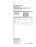
Standard Data Acquisition Program
“SST – SDA”
rev 1.54
29.04.2002
Sea & Sun Technology GmbH / Arndtstraße 9-13 / D-24610 Trappenkamp / Germany
Tel.: ++49 (0) 4323 910913 / Fax: ++49 (0) 4323 910915 / www.Sea-Sun-Tech.com
SST-SDA
user´s manual
TABLE OF CONTENTS
page 2 /57
page
Sea & Sun Technology GmbH ............................................................................................ 1
SST’s Standard Data Acquisition ....................................................................................... 2
Overview............................................................................................................................... 6
Software / OS Demands ...................................................................................................... 6
Hardware / PC Demands ..................................................................................................... 6
Operation.............................................................................................................................. 6
User input............................................................................................................................. 6
Display.................................................................................................................................. 6
Settings ................................................................................................................................ 7
Statusline ............................................................................................................................. 7
Help....................................................................................................................................... 7
Quick link Window ............................................................................................................... 7
Text Windows....................................................................................................................... 8
Textual display of Data........................................................................................................ 8
Text window “Scrolled”....................................................................................................... 8
Text window “Table” ........................................................................................................... 8
Text window “LargeTable”.................................................................................................. 8
Button “Close”..................................................................................................................... 8
Sensor selection dialog for textual display windows, ASCII-Conversion,
Remote Display etc.............................................................................................................. 8
Add a Sensor to List .................................................................................................... 9
Change a Sensor in List .............................................................................................. 9
Delete a Sensor in List................................................................................................. 9
Move a Sensor in List .................................................................................................. 9
Update Rate .................................................................................................................. 9
Graphic Windows .............................................................................................................. 11
Graphical Display of Data.................................................................................................. 11
Graphic Window “XY-Graphic”......................................................................................... 11
Graphic Window “Moving Graphic” ................................................................................. 11
“Virtual” Window ............................................................................................................... 11
Buttons............................................................................................................................... 11
Button “Clear”............................................................................................................ 11
Button “Zoom” ........................................................................................................... 11
Button “Close” ........................................................................................................... 12
Button "Pause" .......................................................................................................... 12
Vertical and horizontal axis....................................................................................... 12
Sea & Sun Technology GmbH / Arndtstraße 9 - 13 / D-24610 Trappenkamp / Germany
Tel ++49 (0)4323 910913 / Fax ++49 (0)4323 910915 / www.Sea-Sun-Tech.com
SST-SDA
user´s manual
page 3 /57
Configuration dialog for the graphic display windows ................................................... 12
Add a sensor to list.................................................................................................... 12
Change a sensor in list .............................................................................................. 12
Delete a sensor in list ................................................................................................ 13
Move a sensor in list.................................................................................................. 13
Colours ....................................................................................................................... 13
Scaling of axis............................................................................................................ 13
Time axis .................................................................................................................... 13
Hint about time........................................................................................................... 14
Line mode................................................................................................................... 14
Line Thickness ........................................................................................................... 14
Grid ............................................................................................................................. 14
Leader ......................................................................................................................... 15
"X-Axis Shown", "Y-Axis Shown"............................................................................. 15
Configure virtual window .......................................................................................... 15
Main Menu .......................................................................................................................... 16
The Menu structure ........................................................................................................... 16
Main menu "File" ............................................................................................................... 16
Main menu "Record" ......................................................................................................... 16
Main menu "Replay" ......................................................................................................... 17
Main menu "External"........................................................................................................ 17
Main menu "Calibrate" ..................................................................................................... 17
Main menu "Display" ........................................................................................................ 18
Main menu "Options" ....................................................................................................... 18
Main Menu “Help”.............................................................................................................. 18
Projects .............................................................................................................................. 19
Concept of a “Project” ...................................................................................................... 19
Configuration Dialog “New Project” ......................................................................... 19
Name of new project .................................................................................................. 19
Description of new project ........................................................................................ 19
Select a COM-port / Select a probe........................................................................... 19
Saving and loading a project..................................................................................... 20
Recording modes .............................................................................................................. 21
Continuous......................................................................................................................... 21
Time Mode.......................................................................................................................... 21
Time Mode Schemas.................................................................................................. 21
Using Start-Time and Stop-Time............................................................................... 22
Increment Mode ................................................................................................................. 22
Trigger Sensor for Increment Mode.......................................................................... 23
Delta Interval .............................................................................................................. 23
use Start value, use Stop value................................................................................ 23
Printing............................................................................................................................... 24
Printer Setup ...................................................................................................................... 24
OnLine Printing.................................................................................................................. 24
Printing of windows contents ........................................................................................... 24
Sea & Sun Technology GmbH / Arndtstraße 9 - 13 / D-24610 Trappenkamp / Germany
Tel ++49 (0)4323 910913 / Fax ++49 (0)4323 910915 / www.Sea-Sun-Tech.com
SST-SDA
user´s manual
page 4 /57
MemoryProbes................................................................................................................... 25
Option Pack: MemoryProbes ............................................................................................ 25
Process: Readout of Stored Data from a MemoryProbe ................................................. 26
Process: Configuration of a MemoryProbe ..................................................................... 27
Buttons and Boxes of the MemoryProbe Window........................................................... 28
Example Processes ........................................................................................................... 30
Data Storage ...................................................................................................................... 30
Enter the Header-Comment............................................................................................... 30
Replay of Stored Data........................................................................................................ 31
Conversion of Raw-data to ASCII-File .............................................................................. 31
Show the Header-Comment .............................................................................................. 32
Show or Edit the Calibrational Coefficients..................................................................... 32
Field Calibration for Air Pressure compensation ............................................................ 32
Field Calibration for Oxygen Sensor ................................................................................ 32
Field Calibration Sensors.................................................................................................. 32
Configuration of Memory Probes ..................................................................................... 33
Import of “*.CNF” Configuration Files.............................................................................. 33
Troubleshooting ................................................................................................................ 34
Program gives error messages after copy to another directory and/or computer........ 34
No Data Displayed ............................................................................................................. 34
Appendix ............................................................................................................................ 35
Contents of a Probe-File ................................................................................................... 35
“Physical” and “Calculated” sensors....................................................................... 35
Calibrational coefficients........................................................................................... 35
The sections of a probe file *.PRB : .......................................................................... 35
Diagnostic Window............................................................................................................ 36
Register Filetypes of SDA ................................................................................................. 36
Actors: Water samplers..................................................................................................... 37
Actors: Remote Control for BioFish................................................................................. 38
Manual mode .............................................................................................................. 38
Automatic mode......................................................................................................... 39
Using a TCP/IP Network for Raw-data Distribution ......................................................... 40
SDA as Server ............................................................................................................ 40
IP-Addresses .............................................................................................................. 40
SDA as Client ............................................................................................................. 40
Server and Client........................................................................................................ 41
Network connections................................................................................................. 41
Sea & Sun Technology GmbH / Arndtstraße 9 - 13 / D-24610 Trappenkamp / Germany
Tel ++49 (0)4323 910913 / Fax ++49 (0)4323 910915 / www.Sea-Sun-Tech.com
SST-SDA
user´s manual
page 5 /57
About the Program ............................................................................................................ 42
About probes, parameters and calibration ...................................................................... 42
List of available Sensor Calculations............................................................................... 44
Raw-data Sensors.............................................................................................................. 44
General Sensor (type "N"ormal ) .............................................................................. 44
Press Sensor (type P) ................................................................................................ 44
Li-Cor sensor, Mantissa part (type NLM).................................................................. 44
Li-Cor sensor, Exponent part (type NLE) ................................................................. 45
Raw-data Range sensor ( 2 Channel , type RR2) ..................................................... 45
Raw-data Range sensor (4 channel , type RR4)....................................................... 45
Normal Field Calibration sensor (type NFC) ............................................................ 46
"ME"-style Oxygen Sensor (type O2)........................................................................ 46
Oxygen sensor "AMT" style, Voltage output [mV] (type VO2) ................................ 46
Calculated Sensors ........................................................................................................... 47
Calc-sensor Bottom ( type 1 or 3 : BOT, BO3 ) ........................................................ 47
Calc-sensor Bottom ( type 2 : BO2) .......................................................................... 47
Calc-sensor Li-Cor-sensor (type LIC) ....................................................................... 48
Calc-sensor Cappa25 (type C25)............................................................................... 48
Calc-sensor Salinity (UNESCO PSS-78, type S)....................................................... 48
Calc-sensor Density anomaly (Sigma-T, UNESCO 1983, type SIT)......................... 48
Calc-sensor Sound velocity (UNESCO svun83, type SVC) ..................................... 49
Calc-sensor Range-switch 2ch (Threshold, type RS) .............................................. 49
Calc-sensor Range-switch 2ch (Switch-sensor bit, type RSB) ............................... 49
Calc-sensor Range-switch 4ch (lower 2 bits of raw-data-sensor, type RS4) ......... 50
Calc-sensor Range-switch 5ch (pointer-sensor, type RS5) .................................... 50
Calc-sensor AMT Oxygen [%] (type O2A)................................................................. 50
Calc-sensor AMT pH-sensor (type PH) ..................................................................... 51
Calc-sensor AMT H2S-sensor (type H2S)................................................................. 51
Calc-sensor AMT Sulphide (type SUL) ..................................................................... 51
Calc-sensor Methane (CAPSUM, type MET)............................................................. 51
Calc-sensor Pressure compensated Oxygen (type OP) .......................................... 52
Calc-sensor Oxygen mg/l or ml/l (types OMG, OML) ............................................... 52
Calc-sensor Water sampler with motor rosette (type 1 and 5 : WS1, WS5) ........... 52
Calc-sensor Water sampler with magnetic releasers (type 2 : WS2)...................... 53
Calc-sensor Velocity direction (type VD).................................................................. 53
Calc-sensor Velocity (compensated by sound velocity, type VS) .......................... 53
Calc-sensor Conductivity estimated from Salinity (type CCS) ............................... 54
Calc-sensor GPS Date and Time (type GDT)............................................................ 54
Calc-sensor GPS Latitude or Longitude (types GLA, GLO) .................................... 55
Calc-sensor Internal Date/Time (type IDT)................................................................ 55
Calc-sensor Polynom (type PLY) .............................................................................. 55
Calc-sensor CAL ........................................................................................................ 56
Calc-Sensor ADD ....................................................................................................... 56
Calc-sensors Difference, Magnetic Direction, Quotient, Product, Velocity ........... 56
Calc-sensor PDU1-time (type PDD)........................................................................... 56
Calc-sensor AMT Oxygen saturation or mg/l ........................................................... 57
Sea & Sun Technology GmbH / Arndtstraße 9 - 13 / D-24610 Trappenkamp / Germany
Tel ++49 (0)4323 910913 / Fax ++49 (0)4323 910915 / www.Sea-Sun-Tech.com
SST-SDA
user´s manual
page 6 /57
SST’s Standard Data Acquisition
Overview
The program allows the Display, Recording und Replay of measurement data from oceanographic multiparameter probe systems of various companies ( at present ADM, ASD, ME, SBE, SST, more to come) as
well as navigational information from GPS-receivers with the NMEA183 standard.
All trademarks mentioned in this user manual are property of their respective owners.
Software / OS Demands
SDA is a program for the 32bit -Windows Systems Win95 (and newer) and Windows NT (and newer). There
are no further requirements regarding the operating system !
The program consists of the SSDA_xxx.EXE file and the project- and probe-related configuration files, no
dll's, no drivers. Even the use of serial ports on extension cards and/or USB is done via the operating
system's application programming interface.
The program itself uses Windows Registry entries only at user request ("Options/Registry/Register file
types") to automatically start SDA at a click on an SDA-related file. The probe- and project files are pure
ASCII text files, all settings can be displayed by the context menu's quick-view function.
.
Hardware / PC Demands
The Hardware-Demands are very moderate, a PC with a 486 CPU with 33MC and 16 MB RAM under Win95
is sufficient for the display and recording even of several probes at the same time !
The program itself uses less than 2 MB of hard-disk space, so most of its capacity can be used by the stored
data of your measurement campaigns.
An installed graphic adapter of type VGA with 640 by 480 pixels is usable, but with more display area work is
something more pleasant. Do think about ergonomics and use CRTs with 17" diameter or more and vertical
sync frequencies of more than 80 Hertz.
LC-Displays of 15" and more than 60 Hertz are sufficient, too.
Operation
User input
SST-SDA can be operated via keyboard or mouse. Its use of menus and dialogs make it suited for operation
even by semi-skilled personnel. Only some basic knowledge of a modern graphical user interface is
necessary. There is context help via the F1 key for almost any situation. For operation in harsh environments
handling exclusively by keyboard is possible.
Display
There are three different text windows and two graphic windows for the representation of the sampled data.
Those windows can be operated simultaneously and independent from each other.
The number of sensors to be shown in each of them is virtually unlimited as are the options for sensor
configuration. Every sensor can be displayed more than once if different numerical representations are
aimed.
All data display windows are sizable. The used fonts are automatically sized when the width of a window is
increased or decreased.
Sea & Sun Technology GmbH / Arndtstraße 9 - 13 / D-24610 Trappenkamp / Germany
Tel ++49 (0)4323 910913 / Fax ++49 (0)4323 910915 / www.Sea-Sun-Tech.com
SST-SDA
user´s manual
page 7 /57
Settings
To ease working with SST-SDA almost all current parameters are stored to the project files at the end of the
program's run (or before the loading of another project). Those are the position and size of the displayed
windows, their respective selected sensors with all their parameters at the last state and the list of recently
used project-files.
At the start of the program only the main window with the menu and the "Scrolled" text window are opened.
By use of the DISPLAY - menu or the Quick-link the selected windows are opened with all the parameters
as they were used last time.
Status line
The Status line at the bottom of the "Scrolled" window is divided into four panels :
Panel 1
Display
Recording
Replay
Replay halted
ASCII Convert
Memory Config.
Program status is displayed, as may be :
Default state, values are displayed only.
Data is recorded, progress is shown in panel 4.
stored data is displayed, progress in panel 4.
dito, paused temporarily
Raw-data file(s) are being converted to text output
A Memory Probe is just being configured or read-out
Panel 2 Name of current loaded project file
Panel 3 Name of last recently used raw-data file
Panel 4 Progress at recording or replay, numbers denominate bytes or percent.
Notice : A mouse-move over panels 2 and 3 of the status line pops up a hint with the full filename including
the path.
Help
By use of the F1–key a context-sensitive help system is installed. If you are unsure what to do in a window or
dialog then press the F1 key (= Function key #1) to gain some help.
There is an index and a find function as well in the help system.
Hints are displayed by moving the mouse over some active areas.
Quick link Window
At the start of the program only the main window with the menu and the "Scrolled " text window are opened.
By use of the DISPLAY - menu or the Quick-link the selected windows are opened with all the parameters
as they were used last time.
Quick-link "Open window / bring to front"
This small window contains checkboxes for all display windows. By a click on the corresponding line the
chosen window opens immediately without the use of the main menu item "DISPLAY ". If the selected
window is open already, then this window is brought to front and gets the focus for operation.
The Quick-link window itself always stays on top of all other windows of SST-SDA and its position can be
moved to a place where it is not covering another window.
Sea & Sun Technology GmbH / Arndtstraße 9 - 13 / D-24610 Trappenkamp / Germany
Tel ++49 (0)4323 910913 / Fax ++49 (0)4323 910915 / www.Sea-Sun-Tech.com
SST-SDA
user´s manual
page 8 /57
Text Windows
Textual display of Data
For the display of the measured data there are three text windows which can be open simultaneously and be
configured independently.
Text window "Table"
Text window "Large Table"
Text window "Scrolled"
Text window “Scrolled”
The main window of SST-SDA shows the main menu and the values of selected sensors. The sensors are
listed side by side and are smoothly scrolled upwards, so that the measured data can be read easily while
they are moving to the top of the screen. About one new dataset per second is written at the bottom of the
window. If the number of sensors to be displayed is larger than the width of the main window, the display
area can be scrolled horizontally without loosing data.
Due to the smooth scrolling the Scrolled window shows only a part of all the datasets that are received (or
replayed) by the computer. To show every dataset at the replay of a file activate the checkbox "Wait for
Scrolled Text" in the replay options dialog !
A Click on the display area or on a sensor-label opens a configuration dialog for the window or this very
sensor.
Text window “Table”
In this table display more information is shown for each sensor : There are the raw-data as integers and the
(via the calibrational coefficients) calculated physical values as well as the corresponding name of the probe,
the sensor and its address and unit.
When the window is enlarged horizontally then automatically a larger font is used so that characters can be
read more easily. The vertical size of the window is dependant on the number of sensors to be displayed.
A Click on the display area or on a sensor-label opens a configuration dialog for the window or for this very
sensor.
Text window “Large Table”
This window with large letters is intended to be looked at from a distance. Even some meters away the
values of the selected sensors can be read with convenience.
When the window is enlarged horizontally then automatically a larger font is used so that characters can be
read more easy. The vertical size of the window is dependant on the number of sensors to be displayed.
A Click on the display area or on a sensor-label opens a configuration dialog for the window or for this very
sensor.
Button “Close”
Closes the current text window. The size, position and other parameters like the list of sensors are saved
and will be active the next time this window is opened.
Sensor selection dialog for textual display windows, ASCII-Conversion,
Remote Display etc.
In this dialog a list of sensors is edited that will be a selection out of all available sensors, physical and
calculated. A single sensor can be entered multiple times, e.g. to be displayed in different textual presentations: engineering, scientific, hexadecimal, binary etc. The length of the list is not restricted.
Sea & Sun Technology GmbH / Arndtstraße 9 - 13 / D-24610 Trappenkamp / Germany
Tel ++49 (0)4323 910913 / Fax ++49 (0)4323 910915 / www.Sea-Sun-Tech.com
SST-SDA
user´s manual
page 9 /57
This window is the general sensor selection dialog of SST-SDA.
A Click on the display area or on a sensor-label opens the configuration dialog for the window or this very
sensor.
Add a Sensor
Change Sensor in List
Delete Sensor in List
Move Sensor in List
Update Rate
Add a Sensor to List
If the list of sensors to be displayed is empty or a new sensor shall be displayed additionally then first the
probe has to be selected. A click on the down-arrow of the list box opens a list with all probes contained in
this project and a click on one of the lines picks the probe.
After selecting the probe the list of sensors is updated accordingly. A click on the down-arrow of the list box
opens a list with all sensors this probe is equipped with. A scroll-bar helps navigating through the list. A
sensor is selected by clicking on it's line in the list box.
At textual representation the display format has to be selected. This is done in the same manner like probe
and sensor were selected. There are display formats with 0 to 4 decimals (engineering format), a 10character or 20-character wide scientific format, some raw-data formats and special formats for time and
GPS- position.
At graphical windows there is only a difference between physical and raw-data ranges, the number of
decimals is of no relevance. For the time "sensor" there is a difference between absolute and relative time.
Finally the sensor can be added by a click on the "ADD" button to the list of displayed sensors.
Change a Sensor in List
A click on one line of the list of displayed sensors in the lower part of the dialog window highlights this sensor
and shows its properties in the lists at the top. One or more of this properties can be changed at will and a
final click on the "CHANGE" button accepts and stores this configuration. The list of sensors is changed
accordingly.
Delete a Sensor in List
A click on one line of the list of displayed sensors in the lower part of the dialog window highlights this sensor
and shows its properties in the lists at the top. A click on the "DELETE" button erases this line in the list of
sensors. The properties of the deleted sensor are stored in memory and can be inserted at any other
position of the list. The list of sensors is changed accordingly.
Move a Sensor in List
A click on one line of the list of displayed sensors in the lower part of the dialog window highlights this sensor
and shows its properties in the lists at the top. A click on the "DELETE" button erases this line in the list of
sensors. The properties of the deleted sensor are stored in memory and can be inserted at any other
position of the list by clicking on another line followed by a click on the button "INSERT". The sensor is
inserted ABOVE the clicked line. If the sensor shall be moved to the very end of the list then after clicking the
"DELETE" button the "ADD"- button has to be clicked instead of clicking "INSERT".
The list of sensors is changed accordingly.
Update Rate
The text windows "TABLE " and "LARGETABLE " have a track bar for "UPDATE INTERVAL". This is set to
0.5 seconds as a default and denotes the rate at that new received measurement data is written to this
window. This time can be expanded up to 5 seconds in divisions of 0.5 seconds. There is no averaging
across this update interval.
Sea & Sun Technology GmbH / Arndtstraße 9 - 13 / D-24610 Trappenkamp / Germany
Tel ++49 (0)4323 910913 / Fax ++49 (0)4323 910915 / www.Sea-Sun-Tech.com
SST-SDA
user´s manual
page 10 /57
The Text window "Scrolled" has a track bar for "Pixel lines to scroll by". This is set to 1 as a default and
denotes the standard smooth scrolling feature of the scrolled window. For some slow computers and / or
slow operating systems this may be to high a burden for the graphic display of the computer (or the software
driver of it), therefore the timing can be selected to be made more suitable to those by grouping single scroll
actions and move from smooth scroll to text line-scroll. Each step of 1, 2, 4, 8, 16 pixel lines doubles the time
between two consecutive scroll actions and releases more resources to other parts of the program. At 16
lines per scroll one complete line of text is scrolled up at a rate of 0.8 seconds per line and effectively
switches OFF the smooth scroll feature.
This may be necessary at Windows NT and successors.
Sea & Sun Technology GmbH / Arndtstraße 9 - 13 / D-24610 Trappenkamp / Germany
Tel ++49 (0)4323 910913 / Fax ++49 (0)4323 910915 / www.Sea-Sun-Tech.com
SST-SDA
user´s manual
page 11 /57
Graphic Windows
Graphical Display of Data
For the display of the measured data there are two graphic windows which can be open concurrently and be
configured independently.
Graphic window "XY-Graphics" and Graphic window "Moving Graphics"
Graphic Window “XY-Graphic”
This static graphic window displays several selected sensors in horizontal axis versus one vertical axis. This
vertical axis can be either time (relative or absolute) or another of the sensors like pressure. The number of
horizontal axis is not limited, but with too many axis you may get confused.
The scaling of each axis can be defined independent from others, the values at the left and right borders are
entered together with the number of major and minor divisions. The colours of the axis can be chosen in a
dialog as well as the colours of the background (canvas) and the optional grid. With Line mode two
consecutive points of sensor data are connected by a solid line.
For special purposes a "virtual window" can be used.
A click on one of the axis or the display area opens a configuration dialog.
Graphic Window “Moving Graphic”
This graphic window simulates a chart recorder on the screen. The "paper", i.e. the graphics moves slowly
across the window writing new lines for the sensors at one edge of the window. The direction of this
movement can be configured to all four borders (left, right, top, bottom). One or more axis, all perpendicular
to the movement direction, can be configured.
For special purposes a "virtual window" can be used.
A click on one of the axis or the display area opens a configuration dialog.
“Virtual” Window
The scaling of axis in charts always is a compromise between resolution and readability. To circumvent this
we defined a virtual window. This can be much larger than the window that is shown on the screen, and we
look "through" this window onto the wider screen with the data displayed. By the means of track bars the
interesting part of the wide screen can be moved so that the graphical data representation of the measured
values becomes visible. The factor by which the wide screen is larger than the window can be defined by a
dialog for X- and Y- axis independently. To automate the operation of the track bar(s) a "leader" sensor for
the horizontal and the vertical axis can be defined, that moves the track bars in a way that the current values
of those sensors are always displayed inside the graphic window on the screen.
Buttons
Button “Clear”
Erases the canvas of the graphic window. The value of relative time is set to zero and for Relative Time Axis
the reference time is set to NOW or - at Data Replay - to the time just displayed on screen.
Button “Zoom”
If virtual window is activated the button "ZOOM" is visible. Clicking on it shrinks the (invisible) wide screen to
the display window's size and displays it. This is done by leaving out some of the pixels of the wide screen
so that the picture fits to the graphic window. The wide screen is still active and can receive data, it is only
mapped to the small window.
The intention of using the ZOOM is just to locate some sensor lines that have got out of focus or getting a
quick overview while using the virtual window .
A second click to "ZOOM" restores the original window.
Use the "LEADER" option for automatic operation of the track bar(s).
Sea & Sun Technology GmbH / Arndtstraße 9 - 13 / D-24610 Trappenkamp / Germany
Tel ++49 (0)4323 910913 / Fax ++49 (0)4323 910915 / www.Sea-Sun-Tech.com
SST-SDA
user´s manual
page 12 /57
Button “Close”
Closes the current text or graphic window. The size, position and other parameters like the list of sensors are
saved and will be active the next time this window is opened.
Button "Pause"
In the Moving Graphic window a click on the "Pause" button temporarily freezes the graphic and changes the
label of the button to "continue". This has no effect on other windows or functions !
Another click on Pause/Continue restarts the moving of the window again. Data received during freeze will
not be displayed.
Changes of axis have to be confirmed by clicking the "CHANGE" button !
Vertical and horizontal axis
At the XY-graphic the first defined axis is interpreted as the vertical axis and all the following ones as
horizontal axis, at the moving graphic window there is only one type of axis.
The number of axis displayed is virtually unlimited, but common sense shows that one should not chose too
many axis as it is hard to differentiate so many colours and lines from each other.
Configuration dialog for the graphic display windows
A Click on the display area or on a sensor-axis opens the configuration dialog for the window or this very
sensor.
In this dialog a list of sensors is edited that will be a selection out of all available sensors, physical and
calculated. A single sensor can be entered multiple times. The length of the list is not restricted.
Add a Sensor
Change Sensor in List
Delete Sensor in List
Move Sensor in List
Colours
Vertical- and Horizontal-Axis
Axis Scaling
Time Axis
Hint about Time
Line mode
Line Thickness
Grid
Leader
"X-Axis Shown" and "Y-Axis Shown"
Virtual window
Add a sensor to list
If the list of sensors to be displayed is empty or a new sensor shall be displayed additionally then first the
probe has to be selected and then the sensor from the list of equipped sensors of that probe and the desired
display format.
Finally the sensor can be added by a click on the "ADD" button to the list of displayed sensors.
Change a sensor in list
A click on one line of the list of displayed sensors in the lower part of the dialog window highlights this sensor
and shows its properties in the lists at the top. One or more of this properties can be changed at will and a
final click on the "CHANGE" button accepts and stores this configuration. The list of sensors is changed
accordingly.
Sea & Sun Technology GmbH / Arndtstraße 9 - 13 / D-24610 Trappenkamp / Germany
Tel ++49 (0)4323 910913 / Fax ++49 (0)4323 910915 / www.Sea-Sun-Tech.com
SST-SDA
user´s manual
page 13 /57
Delete a sensor in list
A click on one line of the list of displayed sensors in the lower part of the dialog window highlights this sensor
and shows its properties in the lists at the top. A click on the "DELETE" button erases this line in the list of
sensors. The properties of the deleted sensor are stored in memory and can be inserted at any other
position of the list. The list of sensors is changed accordingly.
Move a sensor in list
A click on one line of the list of displayed sensors in the lower part of the dialog window highlights this sensor
and shows its properties in the lists at the top. A click on the "DELETE" button erases this line in the list of
sensors. The properties of the deleted sensor are stored in memory and can be inserted at any other
position of the list by clicking on another line followed by a click on the button "INSERT". The sensor is
inserted ABOVE the clicked line. If the sensor shall be moved to the very end of the list then after clicking the
"DELETE" button the "ADD"- button has to be clicked instead of clicking "INSERT".
The list of sensors is changed accordingly.
Colours
The colour of every axis, the background of the graphical windows ("CANVAS") and the optional "GRID" can
be changed at will via a colour dialog. A click on "click here for sensor colour" (twice !!!) opens the colour
selection dialog.
Axis can be scaled by a configuration dialog .
Changes of axis have to be confirmed by clicking the "CHANGE" button !
Scaling of axis
The axis for the graphical display of measurement data can be configured separately for each sensor. The
scaling of the axis is done by defining the left and right border values, the number of major divisions between
them, the minor divisions between the major ones and, of course, the colour of the axis and sensor-lines.
The labelling of the major division marks is done automatically. If the marks appear to be too close together
on the screen, then only those marks are labelled that are at a distance of the width of one label. The left
and right border marks are labelled in any case.
The displayed sensor-lines are a representation of their physical values as long as the defined display format
is some of the floating-point formats. If you want to display the 16 or 20bit integer raw-data of one sensor
instead, then the display format has to be defined as one of the RAW-DATA ones, e.g. RAW_INT.
(Remember that calculated sensors do not have a raw-data value by definition !)
Changes of axis have to be confirmed by clicking the "CHANGE" button !
Time axis
The time is used like one of the other sensors, i.e. there are left and right border limits and major and minordivisions.
The representation of time depends on the language version of your operating system!
There a some options in the properties part of the country-settings that touch the display of data and
time/date !
The standard "time-sensor" is called IDT (Internal Date Time). There can be another time sensor as well: If
there is a GPS-receiver connected, its time sensor is called GDT (Gps Date Time). These sensors both have
two display formats, one is that of the absolute time (e.g. '14:11:23 28.2.1999') denoted by "DATE" and the
other one is that of time elapsed since starting of the graphic window (or the last CLEAR command) called
relative "TIME". The configuration fields change accordingly in the dialog. If the time axis for relative time is
longer than 24 hours, then the field "d" has to be configured with the number of days. At absolute time the
start- and stop day can be selected from a calendar.
Changes of axis have to be confirmed by clicking the "CHANGE" button !
Sea & Sun Technology GmbH / Arndtstraße 9 - 13 / D-24610 Trappenkamp / Germany
Tel ++49 (0)4323 910913 / Fax ++49 (0)4323 910915 / www.Sea-Sun-Tech.com
SST-SDA
user´s manual
page 14 /57
Hint about time
The internal representation of time in the program is that of a floating-point value. The integer part of the
time-value denotes the number of days since 31.12.1899 and the fractional part denotes the relative position
within one day. (e.g. 6:00 in the morning is 0.25, 12 o' clock noon is 0.5 and 18:00 in the evening is 0.75)
As the time is just another floating point value alike the other sensors, it can be displayed in graphics and in
textual windows.
The property "display format" has a slightly different meaning in those two types of windows:
At text windows the display format "DATE" denotes a string showing exclusively the date and "TIME" shows
only the time of day. Therefore the sensor IDT=Internal Date Time (or GDT for GPS) has to be selected
twice in a text-window to show the complete time and date, once with display format "DATE" and once with
display format "TIME" (or TIME+ms) !
At graphic windows the "Display Format" property of the time sensor has a different meaning, as there it is
used to distinguish between two types of axis scalation. The display format "DATE" stands for absolute time
and "TIME" stands for relative time :
Absolute Time: e.g. 'from 14:11:23 28.2.1999 to 10:01:00 2.3.1999'. The "Display Format" of the time
sensor is has to be set to "DATE". At a configuration window the day can be selected from a calendar, the
time has to be entered in the usual hh:mm:ss format. The left and right borders of an axis both have to be set
to (absolute) date and times.
Relative Time: length of time elapsed since an event. At the opening of the graphic window or at the
CLEAR command the relative time is set to zero. The "Display Format" property of the time sensor has to be
set to "TIME". In graphics the left border (most times) is set to zero and the right border has to be entered in
units of hh:mm:ss. If the time axis for relative time is longer than 24 hours, then the field "d" has to be
configured with the number of days.
The differentiation of relative and absolute time is only used with the two graphic windows. The zero setting
of one window does not influence the "relative" time of the other window(s).
See also:
Axis scaling
Time axis
Changes of axis have to be confirmed by clicking the "CHANGE" button!
Line mode
With graphic representation of measurement data it is a standard option to connect two consecutive display
positions of a sensor by a straight line. If this is -for any reason- not wanted, then the checkbox "LINEMODE"
shall be left empty.
Line Thickness
To enhance visibility of a sensor line in one of the graphical display windows the width of this line can be
enlarged. As standard all lines are displayed with a thickness of one screen pixel. The selection box gives a
choice of 1 to 10 pixels. For even thicker lines enter a number in the selection box. Line Thickness is a
property of one single sensor, to enlarge the lines of all sensors, each one has to be set to the desired
thickness. The widening of the sensor lines is only effective with line mode switched ON!
Grid
To ease comparing values on the screen there is the option to lay a grid of dotted lines across the screen.
The color of this grid can be configured by a click on "Select Grid Colour". If this option is not wanted the
checkbox "GRID" should be left empty.
The lines of this grid are always 20 screen pixels apart, they do not change with axis scalation.
Sea & Sun Technology GmbH / Arndtstraße 9 - 13 / D-24610 Trappenkamp / Germany
Tel ++49 (0)4323 910913 / Fax ++49 (0)4323 910915 / www.Sea-Sun-Tech.com
SST-SDA
user´s manual
page 15 /57
Leader
One sensor of the horizontal axis and the vertical axis sensor can be defined as "Leader" sensors with the
XY-Graphics . With the Moving Graphics one of the sensors can be defined as leader. This option shows a
crosshair with one or two lines moving with the current values of those one or two sensors. Each of the lines
has the colour of its corresponding sensor.
If the option virtual window is activated then the definition of these leader sensors moves the wide screen
display in a way that the current values of those one or two sensors are always to be seen in the graphic
window. The track bar(s) are operated automatically in this case.
Changes of axis have to be confirmed by clicking the "CHANGE" button !
"X-Axis Shown", "Y-Axis Shown"
The standard values of both fields is "100%", any other value activates the "Virtual window"
Configure virtual window
The configuration dialog of "XY-Graphics" and "Moving Graphics" windows contains fields for the factors of
X- and Y-axis. As standard those factors are set to "100%", changing this to another value from the popup
list activates the virtual window .
The factors by which the wide screen is larger than the graphic window can be defined for X- and Y- axis
independently from 1 to 10. In case the amount of resources to create the wide screen is too big, then the
factor is reduced automatically to 1.0 and the user may either reduce the size of the window on the screen
or reduce the factor to a smaller value.
Defining a large wide screen may slow down the execution of the program considerably if the PC is not
equipped with enough RAM (less than 32 MB) to store this bitmap picture and so it begins to swap parts of
RAM to disk and vice versa !
To automate the operation of the track bar(s) a "leader" sensor for the horizontal and the vertical axis can be
defined, that moves the track bars in a way that the current values of those sensors are always displayed
inside the graphic window on the screen.
At closing of the window configuration dialog the new values of the factors are adopted.
Sea & Sun Technology GmbH / Arndtstraße 9 - 13 / D-24610 Trappenkamp / Germany
Tel ++49 (0)4323 910913 / Fax ++49 (0)4323 910915 / www.Sea-Sun-Tech.com
SST-SDA
user´s manual
page 16 /57
Main Menu
The Menu structure
The main menu contains the items
FILE,
RECORD,
REPLAY,
EXTERNAL,
CALIBRATE,
DISPLAY,
OPTIONS and
HELP.
Main menu "File"
- New project
Creates a new Project
- Load project
Opens dialog for loading a Project-file "*.SPJ"
- Save project
Writes current status of loaded Project to disk.
- Save project as
saves current Project with different name to disk.
- Printer Set-up
Invokes configuration window of the standard printer
- Print
On Line printing and printing of graphic windows
- Exit program
ends program run, saves currently open data files, too.
1. .. 5.
(List of last recently used Projects, max 5)
A click on one of these loads the project.
Main menu "Record"
- continuous
Switch : every received dataset is stored.
- time driven
Switch : only datasets at defined time intervals are stored.(Time mode)
- value driven
Switch : datasets are stored only when a defined sensor
changes its value more than a given interval limit.(Increment mode)
- Start recording
Starts storage of data to temporary file, at "Stop Recording"
a filename and more information can be entered.
- Stop recording
Stops storage of data, dialog asks for filename to
save temporary file to. Preset is a filename composed from time information at start
of recording. Filename can be changed at will, extension must be *.SRD (default).
Information about the file can be entered into an optional header-comment.
- Edit Header
During or before recording a Header-Comment to
this recording can be entered. At STOP_RECORDING there is a last chance to edit
this text.
Sea & Sun Technology GmbH / Arndtstraße 9 - 13 / D-24610 Trappenkamp / Germany
Tel ++49 (0)4323 910913 / Fax ++49 (0)4323 910915 / www.Sea-Sun-Tech.com
SST-SDA
user´s manual
page 17 /57
Main menu "Replay"
- Start replay
Starts Replay of stored data files, asks for filename and options
for replay.
- Pause replay
Temporarily stops Replay of data.
- Stop Replay
Stops Replay of data, clears windows
- Show Header
During Replay of file : shows comment of this file. Else : shows
comment of selectable raw-data file.
Main menu "External"
The ASCII representation of sensor values can be sent On Line to some other programs or computers by
using different protocols and/or hardware :
- Remote Display
Selection of sensor values to be displayed at an external LC-Display in a watertight
compartment connected via a serial line for use at the winch-operator or else.
- DDE- Server
Selection of sensor values transferred by the Windows(TM) "Direct Data Exchange"
standard to another (DDE-aware) application on the same computer.
- TCP/IP Server
Selection of sensor values transferred by the TCP/IP network protocol to one or
more client-programs on the network.
Notice :
To distribute On Line raw-data via an TCP/IP network the RAW-DATAOUT_ENABLED option of the project
file should be used. To receive raw-data from another probe on the network via TCP/IP the RAWDATAIN_ENABLED option of the project file is intended.
Main menu "Calibrate"
- Press Comp
Field calibration Air pressure compensation
- O2 Field Calib
Field calibration Oxygen slope factor
- Field Calibration Sensors
- Show coeff
Show calibrational coefficients or edit them.
Note : If the current project does not contain such a special sensor the corresponding field calibration menu
item is not shown .
Sea & Sun Technology GmbH / Arndtstraße 9 - 13 / D-24610 Trappenkamp / Germany
Tel ++49 (0)4323 910913 / Fax ++49 (0)4323 910915 / www.Sea-Sun-Tech.com
SST-SDA
user´s manual
page 18 /57
Main menu "Display"
- Table
opens TABLE- window or sets focus on it.
- Large Table
opens LARGETABLE- window or sets focus on it.
- Scrolled
sets focus on the Main window
- XY-Graphic
opens XY-Graphic- window or sets focus on it.
- Moving-Graphic
opens Moving Graphic – window or sets focus on it.
Main menu "Options"
- Actors
Water samplers, Remote Control, etc.
- Memory Probe
readout and configuration of Memory Probes (requires extended version of
SST-SDA)
- Header Vars
A press on the "G" key (while the scrolled window has the focus)
inserts the selected sensor- values into the red field of the Header-Comment.
The purpose of this was to automatically write the GPS -position into the header to
identify measuring stations.
- Export Data file
converts raw-data file (*.SRD, *MRD, *.MER ) into ASCII - Format "*.TOB"
- Import config.
converts ME- "*.CNF" files into project ( *.PRB + *.HDR + *.SPJ)
- Diagnosis
shows information about the current project and the serial ports
- Registry
file types used by SDA (*.PRB, *.SPJ, *.SRD) can be registered
in Windows(tm) so that double-clicking on such a file will start SDA with the clicked
project and/or raw-data file. The options “Run SDA” and “edit xxx-file” are added to
the context-menu (= right mouse-button).
Main Menu “Help”
click on menu "help", click on submenu "Online Manual"
At the very first time help is called Windows cannot find the help file for SSDA_xxx.EXE, so it asks for the
corresponding help file:
Confirm the question with "yes", then point to directory
"C:\SST_SDA" (or wherever SDA is located), double-click on the subdirectory "help"
and the file "ssda.hlp" and click on "open file". From now on Windows connects this help file with SSDA.
At any time in the program a press on the "F1" key opens a window with (context sensitive) help information.
Browse through the Online-Manual to get acquainted with SSDA.
Some standard processes like data storage etc. are explained in chapter "Some Processes".
You can leave open the Help-window during work with the program.
The Help Menu contains:
- On Line Manual
- Index
this manual is available as a help file.
shows a list of keywords or the first page of the help file. At the help file three more
options appear : contents, index and search.
- Using help
opens the “help on help” feature of the operating system
- About.
gives credits to the manufacturer of SDA and lists telephone numbers and
company’s address as well as the revision number of the software.
Sea & Sun Technology GmbH / Arndtstraße 9 - 13 / D-24610 Trappenkamp / Germany
Tel ++49 (0)4323 910913 / Fax ++49 (0)4323 910915 / www.Sea-Sun-Tech.com
SST-SDA
user´s manual
page 19 /57
Projects
Concept of a “Project”
The identification of the probe(s) connected to the system and the status of the display windows with all their
parameters are summarized by the concept of a "project". It describes which probe is connected to which
serial port of the PC, what the selected sensors for display in the various windows are and how their
parameters were adjusted at the time this project was used the last time. There can be several projects for
different campaigns with the same probes denoting e.g. axis scalation corresponding to the measurement
environment. The current status of a project can be saved under another name for special purposes. These
project files are not static, they describe the status of the system at that very time when the project file was
(loaded and) left last time.
The configuration and parameter-settings of SST-SDA are stored in three types of initialisation files :
The configuration of one probe is stored in a "Probe"-file ("*.PRB") . The sensors of this probe are listed
here and the properties of the serial protocol of this probe.
A Project-file "*.SPJ" (Sda-ProJect) contains the references to the connected probes and the properties of all
windows.
The "INI"-file of the program itself contains the list of the five last used project files. At every start of SSTSDA the latest project is loaded automatically.
Notice :
The information about the connected probe(s) are given only as reference in the project file, therefore the
effects of a field calibration of one sensor are available on every project that references this probe thereafter.
No loading etc. is necessary !
Configuration Dialog “New Project”
A click on the menu item "FILE / New Project" opens a dialog for the input of name, description and the
assignment of probes to serial ports. This project is saved to disk with a choosable filename as a "*.SPJ" file.
Name of new project
The name entered for the project can be used as a filename for the project, too. You are free to enter a
different filename at the end of configuration . The name of the project is written to the project file "*.SPJ", but
the project is always referenced by the filename.
Description of new project
This short description of the project is written to the project file "*.SPJ". It may help for a context to the use of
this project.
Select a COM-port / Select a probe
At first the serial port to which the (first) probe is connected is selected from the popup list. Next the probe is
selected after clicking the button "Select a probe". A filename dialog opens and displays all the available
probe files (*.PRB) . You may change directories or even drives at will. As standard the probe files are
situated in the subdirectory "config" of the program. After selecting the probe file the button "OPEN" is
clicked. In the summary field in the lower part of the window now a new line emerges with the COM-port and
the probe filename listed.
If more than one probe at a time shall be connected to the PC then this procedure has to be done again for
every probe. The program supports a maximum of four serial ports at this time, but most PC's are only
equipped with two of them, though.
Additional COM-Ports of plug-in cards, PCMCIA or CARDBUS adapters can be used as well as USBconnected external COM-boxes. (USB functionality requires an operating system of Windows(TM) 98 second
edition or newer).
Sea & Sun Technology GmbH / Arndtstraße 9 - 13 / D-24610 Trappenkamp / Germany
Tel ++49 (0)4323 910913 / Fax ++49 (0)4323 910915 / www.Sea-Sun-Tech.com
SST-SDA
user´s manual
page 20 /57
Saving and loading a project
When all the input for the list of probes in this project is completed then the button "Save as" is clicked and a
name shall be given in a save-file dialog. There is a default filename given from the name of the project, but
you can decide to use any other name. The extension *.SPJ is added and the file is saved.
A confirmation dialog is shown whether the just created project shall be loaded at once. You can decide to
do this or load the project later by the file menu "Load Project".
The basic configuration of a project is complete now. When this project is loaded the first time, you can
select the sensors to be displayed in the text- and graphic windows. To open a new display window use the
item DISPLAY from the main menu of SST-SDA or click on a line of the QUICKLINK window. The first time
you open a window there are no sensors defined so automatically a configuration dialog opens where you
can select the sensors of choice. All entered configuration information is automatically written to file at the
exit of program.
Sea & Sun Technology GmbH / Arndtstraße 9 - 13 / D-24610 Trappenkamp / Germany
Tel ++49 (0)4323 910913 / Fax ++49 (0)4323 910915 / www.Sea-Sun-Tech.com
SST-SDA
user´s manual
page 21 /57
Recording modes
Continuous
Every dataset from any of the connected probe(s) send to SDA are stored on disk.
Time Mode
Data can be stored on a time scale by using time mode to reduce the amount of occupied capacity for the
measured data. There are several schemas available for time mode data storage. The simplest is to store
just one dataset at each time interval, but there are more complex schemes to suit the needs of a
measurement campaign. The Interval Time, On Time and Cycle Time can each be set individually. Some
modes include averaging.
SDA offers these time modes:
1: store one sample at each interval time
2: store all samples during ON-time at each interval
3: store samples with cycle-time during ON-time at each interval
4: store average of samples across interval time
5: store average of samples across ON-time at each interval
6: store avg. of samples across cycle-time during ON-time at each interval
Optionally a Start-Time and/or a Stop-Time can be set.
When this window is used for the configuration of Memory Probes not all options may be available
depending on the class of the probe
Time Mode Schemas
SDA incorporates 6 schemes for time mode :
1: store one sample at each interval time
After one time interval has passed one dataset is measured and stored.
2: store all samples during ON-time at each interval
At each time interval the data storage is on for the On Time. ALL sampled datasets are stored during this
time.
3: store samples with cycle-time during ON-time at each interval
At each time interval the data storage is on for the On Time. During this time after every Cycle Time one
dataset is stored.
4: store average of samples across interval time
After one time interval has passed one dataset is stored that is the average across all sampled data during
the interval.
5: store average of samples across ON-time at each interval
At each time interval the data storage is on for the On Time. The average across all sampled datasets
during this time are stored in one dataset.
6: store avg. of samples across cycle-time during ON-time at each interval
At each time interval the data storage is on for the On Time. During this time the averaged data across
each Cycle Time is stored in one dataset per Cycle Time.
Sea & Sun Technology GmbH / Arndtstraße 9 - 13 / D-24610 Trappenkamp / Germany
Tel ++49 (0)4323 910913 / Fax ++49 (0)4323 910915 / www.Sea-Sun-Tech.com
SST-SDA
user´s manual
page 22 /57
A graphical representation of the principles of the time mode schemas is given in the upper part of the time
mode configuration window. On a time line from left to right the options for the currently displayed time mode
are given in a simplified way. The small green lines above the time line represent the datasets sampled at
normal speed of the probe. The small red lines beneath the time line represent the datasets that would be
stored by this type of time mode. A triangle stands for averaging across a time length.
The graphic shows what Interval Time, On Time and Cycle Time stand for. Interval Time is the time between
two consecutive starts of data storage episodes. It is independent from On Time, which is the time during
that data storage is ON after another Interval Time has passed.
When this window is used to configure some Memory Probes of various vendors, remember that some
classes of Memory Probes do not support all of the above time mode schemas. With Memory Probes On
Time is the time for that the probe is switched on and samples data, part or all of which may be stored.
Using Start-Time and Stop-Time
Time mode data sampling can be further restricted by setting a Start-Time and / or a Stop Time. Start-Time
is the time when the first interval time begins and the first data are stored. When Stop-Time is passed,
recording is terminated instantly (irrespective of any ON-Time etc. !) and the program asks for a filename etc.
Clicking at each of the checkboxes "use Start Time" and "use Stop Time" opens a field to enter the
respective time limits. The date field offers a calendar by clicking on the down-arrow of the field.
With most Memory Probes setting a Start-Time is mandatory and cannot be clicked off. Setting Stop-Time is
not necessary (but useful) on some probes or modes.
Increment Mode
Increment mode is used to store data only at pre-defined value limits. It is mostly used to obtain depth
profiles. e.g. the probe data is stored at every dBar in shallow lakes or every 10 dBar at deep ocean profiles.
The reference sensor for these profiles would be the pressure sensor, here it is called the "Trigger-Sensor"
as it triggers the storage of a dataset. If the project contains more than one probe, the "Trigger-Probe"
(where the trigger sensor is situated) has to be set. The values of this sensor are constantly monitored by the
program. The interval between any two limits has to be defined (Delta interval), it always has to be positive !
A Start-limit and / or an End-limit can be defined to further reduce the amount of data that is stored.
Three different strategies for "crossing the border" can be selected :
trigger at increasing values
trigger at decreasing values
trigger if value has changed in either direction
With the first two modes the first reach of a limit triggers the storage of one dataset, the value may fall back
and cross the limit again WITHOUT triggering ! Once a limit is crossed, the dataset is stored, the next limit is
calculated and after this moment the value has to cross this new limit to trigger storage again.
With the third mode calculations of the next limits (upper and lower) are depending on the current limit
reached : The next upper limit is one delta-interval above the current limit and the next lower limit is one
delta-interval beneath the current limit. If the value of the trigger sensor changes for an amount of one deltainterval in either direction a dataset is stored and this limit is the centre of the next upper and lower limits. As
long as the value of the trigger sensor stays in this space that is two delta intervals wide, no more trigger is
executed.
Start- and Stop limits cannot be used with the third mode.
When this window is used for the configuration of Memory Probes not all options may be available. Some
Memory Probes offer an increment mode, but it is most times restricted to the pressure sensor as the Trigger
Sensor.
Sea & Sun Technology GmbH / Arndtstraße 9 - 13 / D-24610 Trappenkamp / Germany
Tel ++49 (0)4323 910913 / Fax ++49 (0)4323 910915 / www.Sea-Sun-Tech.com
SST-SDA
user´s manual
page 23 /57
Trigger Sensor for Increment Mode
Storage of data during increment mode depends on the current value of one sensor. This sensor is called
the trigger sensor, as its value triggers the storage of data. In SDA this can be any sensor, physical or
calculated.
The trigger sensor is selected by first choosing the probe it is connected to. When there is more than one
probe connected to the system a list of the available probes is opened by clicking on the down-arrow of the
list field labelled "Select a probe ". The probe is selected by clicking on the respective line.
The list of sensors this probe is equipped with is now listed under "Select a sensor". Choose one out of this
list by clicking on the respective line.
Now the values of the delta interval etc. have to be entered. See Delta Interval.
When this window is used to configure some Memory Probes of various vendors the type of sensor used as
trigger sensor may be restricted to the pressure sensor or otherwise.
Delta Interval
At Increment mode data storage is done at pre-defined limits of the value of the trigger sensor. The distance
between two of those limits is called the Delta Interval. This is a positive number ( ! ) that has to be entered
in the edit field. If storage shall be done at decrementing values then the Increment Mode has to be changed
to "decrementing" but the delta interval stays to be a positive number! The value is interpreted in units of the
selected trigger sensor.
use Start value, use Stop value
In Increment Mode datasets are stored at pre-defined value limits. To further reduce the amount of
measured data, Start- and Stop-levels can be defined to store data only if the value of the trigger sensor is
between those levels AND has just crossed a limit. Outside this value span no data is stored. The
checkboxes "use Start value" and "use Stop value" can be clicked independently, so there need not be a
start value to use the stop value limit. Clicking at each of the lines opens a field to enter the respective value
limits.
At incrementing mode the start limit has to be smaller than the stop limit, at decrementing mode the start limit
has to be greater than the stop limit !
At the third mode no start- or stop limits can be defined.
Sea & Sun Technology GmbH / Arndtstraße 9 - 13 / D-24610 Trappenkamp / Germany
Tel ++49 (0)4323 910913 / Fax ++49 (0)4323 910915 / www.Sea-Sun-Tech.com
SST-SDA
user´s manual
page 24 /57
Printing
Printer Set-up
This option invokes the operating system's set-up dialog for the installed printer. See the manual of the
printer and/or the operating system for details of this dialog. This dialog should be called before any printing
activities are invoked.
On Line Printing
A set of selected sensors can be printed on a protocol printer at constant time intervals. A click on main
menu FILE , submenu PRINT and the item "Start On Line Protocol" opens a configuration window for a
selection of sensor-values that shall be printed in one line of the protocol.
The length of the time interval should be set to a convenient value. If the update interval is too short, the
printer may not catch up with the printing. For protocol purposes a page-oriented printer is no good choice,
as the page will be printed only at the completion of one page by the operating system. Old-style lineoriented printers or special systems are a better choice.
To stop On Line printing, the same submenu item now called "Stop On Line Protocol" has to be clicked.
During On Line printing no printing of textual or graphical windows is allowed and vice versa.
Printing of windows contents
The contents of a "Scrolled", "Graphics _XY" or "Moving Graphics" window can be sent to a connected
printer as a hardcopy function. A click on main menu FILE , submenu PRINT and the selected window type
immediately catches the graphic bitmap (=canvas) of the window and sends it to the operating system's
printing device. The outer border of the window and it's buttons etc. will not be included.
If the option "virtual window" at Graphics-XY or Moving Graphic is selected, the printout will show the
complete content of that window, not only the small part that can be seen on the screen !
Additionally the content of the selected window can be saved as a *.BMP Bitmap file, if the option "Save
Graphic as BMP, too" (in the same submenu) has previously been selected.
*.BMP files can easily be shown and edited by tools included in the operating system.
Sea & Sun Technology GmbH / Arndtstraße 9 - 13 / D-24610 Trappenkamp / Germany
Tel ++49 (0)4323 910913 / Fax ++49 (0)4323 910915 / www.Sea-Sun-Tech.com
SST-SDA
user´s manual
page 25 /57
Memory Probes
Option Package: Memory Probes
The Option Package "Memory Probe" is an extension of the standard SST-SDA program. It enables the
configuration and data readout of various Memory Probes from different vendors from inside SST-SDA in
one uniform user interface.
Supported are Memory Probes from :
ADM Elektronik
ASD Sensortechnik
ME Meerestechnik Elektronik GmbH
SBE Sea-Bird Electronics, Inc.
SST Sea & Sun Technology GmbH
( this list will be growing by the time)
Memory Probes are data acquisition systems with internal storage capabilities. The configuration of these
types of oceanographic probes and the readout of their stored data can be done either by removable mass
storage devices or by means of a serial communication and a (proprietary) serial line protocol. Most vendors
use the serial cable version, as opening the probe at sea and getting a mass storage device in and out of the
probe is a risky task in such an environment. The command sets and protocols usually differ from probe
class to probe class, even at probes from the same manufacturer. Therefore the programs to configure and
to retrieve data are as diverse as the probes.
To circumvent the shortcomings of this status SST did a different approach : The functions of the probes
were abstracted from the very probes to a uniform user interface and all differences in protocol etc. are
hidden from the user. Only the abstract functions of readout, configuration, status etc. are shown to the user
in the usual Windows(TM) way of graphical user interface. The user need not know what type of Memory
Probe he is actually dealing with, he just operates the probe by the abstract functions.
In sequence of working with the probe these basic functions are :
Switch memory probe to command mode. Get the current memory status of the probe.
If any data is stored, retrieve it and store it on disk as a compatible binary data file (*.SRD). Add a headercomment to the disk-file to store some text- information with the file.
Set new storage mode. Set options and parameters of this mode. Transfer new configuration information to
the probe.
End command mode. Switch back to standard mode or switch OFF.
By these four functions almost any probe can be dealt with.
Notice:
Storage and configuration of Memory Probes should not be mistaken with storage and recording modes of
SST-SDA for direct reading probes, though most of the configuration windows are similar !
Memory Probes use their own internal mass storage (which has to be read-out by SDA to display it) whereas
data from direct-reading probes is directly stored by SDA on the mass storage devices of the PC.
Sea & Sun Technology GmbH / Arndtstraße 9 - 13 / D-24610 Trappenkamp / Germany
Tel ++49 (0)4323 910913 / Fax ++49 (0)4323 910915 / www.Sea-Sun-Tech.com
SST-SDA
user´s manual
page 26 /57
Process: Readout of Stored Data from a Memory Probe
Data Readout is done in 5 steps:
Switch memory probe to command mode
Get the current memory status of the probe
If any data is stored, retrieve it and store it on disk as a compatible binary data file (*.SRD)
Add a header-comment to the disk-file to store some text- information with the file
End command mode. Switch back to standard mode.
To get to the Memory Probe window click on main menu item OPTIONS, then on MEMORY PROBE and
select the probe that shall be dealt with. When there is only one Memory Probe in this project, there is only
one item to select.
The window opens and shows some buttons and progress bars. The title of the window says "Memory Probe
Configuration for < xxx >" with "xxx" replaced by the identification of the probe. The line below verifies the
type of memory probe that is the class of memory probes this one is part of. The communication protocol that
is used for configuration of this probe is extracted from the name and vendor of the probe.
Only two buttons are enabled at this time : "Start communication" and "Close".
Clicking on "Start communication" will switch the memory probe to command mode and retrieve the current
status of the probe.
The status tells the last used storage mode (Continuous, Time- or Increment operated) and the amount of
data that had been stored in the probe's memory. Some probes can store more than one cast at a time,
some probes use internal averaging of data and some probes have additional status flags regarding battery
status or memory full warning etc. The existence of these data is vendor- dependant and changes from
probe class to class.
If any data at all is stored in the probe's internal memory then the button "Readout Data" is enabled and a
click on this button will start the process. With most probes the transfer of data is done by retrieving blocks of
constant or variable length.
To show the progress of readout there are two separate progress bars at the left top of the window. The
upper one is block-oriented, i.e. it shows the progress of one single block to be transferred. The lower one
shows the progress of the whole process. As this process can take some time with high capacity probes or
with slow communication Baudrates of some probe classes, there may be no or only small progress with the
lower progress bar. The readout of a full capacity data file will take from a quarter of an hour up to one hour
of time. Relatively slow computers and/or operating systems may add significant time to this process.
The retrieved data is first written to the memory of the PC. At the end of the readout process the user is
asked for a filename of the one or more files to write. The default filename is composed from year, month,
day, hour and minute of the day. This filename and the directory the file will be written to can be changed at
will. The extension of the filename is automatically set to "*.SRD" to identify this as an 'SST 'RawData' file.
A header-comment can be added to the file. In case of more than one file to write, the header of each file
can be edited differently. At large volume measurement campaigns the header can be preset at some places
with constant text inputs (Message box "Store this header as a template ?"). These are stored in a file with
the name of the project and the extension "*.TMP". To recover the status with no preset texts this file has to
be deleted.
Readout of data is complete now. If no immediate reconfiguration of the probe for the next measurements is
intended, then the button "Switch-off probe" shall be clicked to leave the command mode and bring the probe
to an energy saving state.
With some classes of Memory Probes the button "Restart Probe" can be used to switch the probe to On Line
mode (without storage of data). The probe in this mode works like a standard direct reading probe. The
"Restart Probe" button my be used only AFTER the "Switch-off probe" button!
When the probe is back from command mode, the button "Close" is re-enabled and can be clicked to leave
the Memory Probe readout process and shut the Memory Probe configuration window.
See also :
Process : Configure a Memory Probe for data storage
Time mode configuration
Increment mode configuration
Sea & Sun Technology GmbH / Arndtstraße 9 - 13 / D-24610 Trappenkamp / Germany
Tel ++49 (0)4323 910913 / Fax ++49 (0)4323 910915 / www.Sea-Sun-Tech.com
SST-SDA
user´s manual
page 27 /57
Process: Configuration of a Memory Probe
Configuration is performed in 5 steps:
Switch memory probe to command mode
Get the current status of the probe
Set new storage mode
Transfer new configuration information to the probe
End command mode. Switch back to standard mode.
To get to the Memory Probe window click on main menu item OPTIONS, then on MEMORY PROBE and
select the probe that shall be dealt with. When there is only one Memory Probe in this project, there is only
one item to select.
The window opens and shows some buttons and progress bars. The title of the window says "Memory Probe
Configuration for < xxx >" with "xxx" replaced by the identification of the probe. The line below verifies the
type of memory probe that is the class of memory probes this one is part of. The communication protocol that
is used for configuration of this probe is extracted from the name and vendor of the probe.
Only two buttons are enabled at this time : "Start communication" and "Close".
Clicking on "Start communication" will switch the memory probe to command mode and retrieve the current
status of the probe. (With some probe classes the probe has to be in the OFF state to start communication !,
check manual of the probe.)
The status tells the last used storage mode (Continuous, Time- or Increment operated) and the amount of
data that had been stored in the probe's memory.
If there is data stored in the probe that has not been previously saved to disk, abort new configuration and
first readout the stored data ! There is NO WAY to get old data AFTER a new configuration has been
initiated !
Some probes can store more than one cast at a time, some probes use internal averaging of data and some
probes have additional status flags regarding battery status or memory full warning etc. The existence of
these data is vendor- dependant and changes from probe class to class.
The last used storage mode is shown in an info-box at the right middle of the window. One of the modes
listed there is selected and is preset for the next storage operation. The button below this box is labelled
"Configure <lastmode> mode" with <lastmode> replaced by one of the modes this vendor's Memory Probe is
supporting.
The operation modes supported by SST-SDA are
Time mode
Increment mode (Pressure mode)
Continuous mode
Event mode
Remember : not all probe classes support all the listed operation modes ! Only valid operation modes are
available in the actual configuration windows.
A click on one of the supported mode lines in the box sets the next operation mode of the probe. The
configuration button below the box changes it's text accordingly.
After clicking on the configuration button a warning message box opens. This is the last chance to abort new
configuration and save previously stored data by use of the "Readout Data" button. At positive confirmation
of the message box the data memory of the probe will be erased !
Depending on the selected operation mode configuration windows will appear. (These are similar to those
used by the SDA program itself to configure storage for direct-reading probes.)
Select the appropriate options and parameters in those windows. (There is no configuration window for
Continuous mode.) If available, select averaging modes etc. in the checkboxes of the status box. These are
editable only at this time.
Sea & Sun Technology GmbH / Arndtstraße 9 - 13 / D-24610 Trappenkamp / Germany
Tel ++49 (0)4323 910913 / Fax ++49 (0)4323 910915 / www.Sea-Sun-Tech.com
SST-SDA
user´s manual
page 28 /57
When all options and parameters are set, the new configuration information shall be transferred to the probe
by the button "OK, send config to probe". If instead you wish to abort the new configuration, press "Abort
config" and the configuration data is NOT sent to the probe. ( Maybe you just wanted to do some training on
the various modes ...)
After the configuration is sent to the probe it is activated by the button "Switch-off probe". This leaves the
command mode and brings the probe to an energy saving state.
Now configuration is complete. With time mode the probe will automatically switch-ON at the configured time
and start storing measurement data. At increment mode and continuous mode the probe has to be switched
on by hand with some actuator. Some classes of probes use a magnetic stick as an actuator and a Reed
switch inside the probe for switch-ON and switch-OFF.
With some classes of Memory Probes the button "Restart Probe" can be used to switch the probe to On Line
mode (without storage of data). The probe in this mode works like a standard direct reading probe. The
"Restart Probe" button my be used only AFTER the "Switch-off probe" button!
When the probe is back from command mode, the button "Close" is re-enabled and can be clicked to leave
the Memory Probe readout process and shut the Memory Probe configuration window.
See also:
Process: Configure a Memory Probe for data storage
Process: Readout of Stored Data from a Memory Probe
Time mode configuration
Increment mode configuration
Buttons and Boxes of the Memory Probe Window
The individual buttons and boxes are not enabled all the time, only at that time the current context allows
using them.
Button "Start Communication"
After opening the Memory Probe window this should be the first button to click. Remember that some
classes of probes need to be in the switched-off state to properly respond to this button. Check the manual
of the probe for further information. Clicking the button will switch-on the probe and/or switching it to
command mode. On some probes the Baudrate of the serial line is automatically switched to another value
for this communication.
Button "Readout Data"
If there is any data stored inside the probe this should be the next step to be done. When the data has
already been read out in a previous session or is of no interest to the user, it can be skipped.
Button "Configure xxxx mode"
After selecting the mode for the next measurement campaign (see Selection Box "Last Configuration") this
button changes its text to the selected storage mode. When clicked, it first invokes the internal function
"Erase old Data" and then opens a window for either time mode or increment mode configuration. For
continuous mode no extra window is opened. After finishing the basic configuration window further
parameters may be entered in the Selection Box "Status of Probe", that is editable at this time.
Button "Switch-off Probe"
To switch a Memory Probe back to standard mode or activate the settings after configuration, the command
mode has to be left by this button. This should be the last button before using the "Close" button. If a new
configuration has be initiated, a protocol file will be written to the directory of the *.EXE file of SDA with the
name of MEMORY_1.TMP. The digit "1" may be replaced by another digit if more than one Memory Probe is
connected to this project. The protocol file is readable ASCII text and logs the time of configuration and the
parameters that had been entered.
Button "Restart Probe"
Some classes of Memory Probes can be awakened by the sending of a single character on the serial line to
restart the probe as a replacement of waking up the probe by the magnetic stick.
Sea & Sun Technology GmbH / Arndtstraße 9 - 13 / D-24610 Trappenkamp / Germany
Tel ++49 (0)4323 910913 / Fax ++49 (0)4323 910915 / www.Sea-Sun-Tech.com
SST-SDA
user´s manual
page 29 /57
Button "Close"
The name is the function, additional it tries to switch-off the probe if this has not already been done by
"Switch-off Probe", before closing the window and returning to the main window of SST-SDA.
.
Button "Abort config"
If the user decides that the configuration parameters he just had completed where not those he intended to
enter, this is an easy way to abort the process and try again.
Button "OK, send config to probe"
By clicking this button the configuration parameters that just had been completed are transferred to the
probe via the serial line. On some probes the very configuration is activated at "Switch-off Probe", so this is
the next button to click.
Selection Box "Last Configuration"
After reaching command mode by "Start Communication" the last used operation mode is read from the
probe and the corresponding line is selected at this selection box. To change this value for a new
configuration another line has to be selected by clicking on that line. The text of the "Configure xxxx mode"
button below this selection box is changed accordingly and a click on it will start entering parameters for this
new configuration.
Selection Box "Status of Probe"
After reaching command mode by "Start Communication" the current status information of the connected
memory probe is read and the corresponding checkboxes and edit fields are filled with that information. At
this time all fields are read-only.
During the new configuration process and after the parameter windows are closed, some of the checkboxes
may be changed by clicking on them and some edit-fields are no longer read-only. After entering the
intended options the next button will be "OK, send config to probe".
Selection Box "Raw-data output during data storage"
Some classes of Memory Probes have the option for different output ports for the On Line raw-data values
during the process of the internal storage. After reaching command mode by "Start Communication" the
current status information of the connected memory probe is read and the corresponding checkbox is
activated. At this time the checkboxes are read-only. During the new configuration process and after the
parameter windows are closed, the checkboxes may be changed by clicking on them for the intended output
port. (None, FSK, V24=RS232)
Checkbox "Verbose Status Messages"
Clicking on this line opens a (sizable) diagnostic window where additional information of the current subfunctions are listed. It is primarily intended for debugging purposes if a probe does not act as supposed.
Using it may confuse some users, but it is a valuable tool for tracing down erroneous behaviour and bugs.
Sea & Sun Technology GmbH / Arndtstraße 9 - 13 / D-24610 Trappenkamp / Germany
Tel ++49 (0)4323 910913 / Fax ++49 (0)4323 910915 / www.Sea-Sun-Tech.com
SST-SDA
user´s manual
page 30 /57
Example Processes
In the following some processes are described as a whole to ease the use of this program. Details of the
menus used are declared in their respective chapters of this manual.
Data Storage
Enter the Header-Comment
Replay of Stored Data
Conversion of Raw-data to ASCII-File
Show the Header-Comment
Show or Edit the Calibrational Coefficients
Field Calibration for Air Pressure compensation
Field Calibration for Oxygen Sensor
Import of “*.CNF” Configuration Files
Data Storage
Click menu RECORD, Item START RECORDING. From now on all received data from all defined probes in
the loaded project will be stored to disk. Panel 1 of the Status line shows "Recording" and in panel 4 of the
Status line the number of bytes already stored is shown. (Notice : Panel 4 of the Status line is shown only
when the main window is wide enough).
Measurement data is at first written to a temporary file that is renamed or copied later. To end recording the
menu item "Stop Recording" is clicked. A confirmation dialog asks to re-edit the Header-Comment of this
file.
Now the new name of the recorded data file is asked by a save-dialog. There is a default filename coded
from data and time of the start of recording. You can accept this filename or enter another one of your choice
and confirm by clicking "OK". If writing to disk of the data is no longer wanted, then you can click "Abort" and
answer the final confirmation dialog "Do you really want to abort saving data ?" with YES.
Data is saved now, if you wanted it, and the filename is written to the panel 3 of the Status line . A following
"REPLAY " command will give you this filename as a default.
Data files have the “Read-Only” attribute set.
Notice
The *.SRD raw-data files are written to disk with the "Read-Only" attribute set to ensure that no accidental
corruption of valuable data can be done. An editor (preferably Notepad.exe or the Quick view item of the
context menu) may be used to view the header part of the raw-data file, but no actual editing is allowed as
this would completely corrupt the binary raw-data part of the file and make the file unusable !
Enter the Header-Comment
The header-comment of a data file stores information about the circumstances of this very measurement, as
can be operator, geographical position, weather, environment or what else. If the current loaded project does
not own a header file "*.HDR" then the header of some other project can be imported via a file dialog box.
The header edit window shows three types of elements :
plain text as labels for information
several blue edit fields for the user to enter information
one red edit field for information that may be interpreted as part of a data filename
The user can enter his information only into the blue or red edit fields, the rest of the screen cannot be
accessed. To enter new text to this fields the existing text (or white space) has to be erased via the DEL- or
Backspace keys. A double click to an edit field marks the text and then the first letter to be entered erases
the whole edit field. The user can jump from edit field to edit field by the use of the TAB key (backward with
shift-TAB).
After completing this input formular the header is closed by a click on the "X" border-icon of the window. If
the entered text ( or large parts of it ) shall be used for future measurements in a campaign, the entered text
can be saved to disk as a default header text. A message box asks for this by "Save this header Y/N ?".
Even a NO writes the current header to the currently recorded data file, but a YES saves the text as a layout
to disk in a "<projectname>.TMP" file. This layout can be changed at any time!
Sea & Sun Technology GmbH / Arndtstraße 9 - 13 / D-24610 Trappenkamp / Germany
Tel ++49 (0)4323 910913 / Fax ++49 (0)4323 910915 / www.Sea-Sun-Tech.com
SST-SDA
user´s manual
page 31 /57
Replay of Stored Data
Click at Menu REPLAY item START. A filename dialog is opened with the last used data filename as a
default. You can browse through files and directories for your file of choice. SST-SDA supports several data
file formats for replay. Standard is *.SRD, but also most files created by the DOS-program "Multipar" can be
read directly. There will be more formats to be read in the future.
The current loaded project has to be compatible with the sensors logged in the data file. The calibrational
coefficients for calculation of the physical values can be read either from the data file or from the current
project. This can be selected in the "REPLAY OPTIONS" dialog after selecting the data file. There are
checkboxes, too, for the clearing of all text- and graphic-windows before the start of replay and for the option
that ALL datasets are shown in the scrolled text window. Normally the scrolled text window gets new data
only when it has scrolled up the last line of data, irrespectively how many datasets were displayed by the
other windows in the meantime, so clicking the option "Wait for scrolled text" makes replay really slow !
To speed up replay by data reduction you can use a data rate higher than 1, either by selecting the factor
from the list box or by directly entering a number in the combo-field. If selected, the program only displays
every n-th dataset.
Replay can be aborted at this point by clicking the respective button.
Clicking "OK. show" starts the replay of data on all open text- or graphic windows. The progress in percent
and bytes is shown in the panel 4 of the Status line and the filename of the data file in panel 3.
Replay can be halted temporarily by menu "REPLAY ", item PAUSE and continued by again clicking this
item now called "Continue". The replay can be stopped premature by menu "REPLAY ", item STOP.
After the file is replayed completely (or was aborted) you can choose to retain the graphical and textual data
on the screen in a confirmation dialog or to clear all windows before new online- or replayed- data is
displayed.
During replay you can have a look at the header-comment of this data file by clicking menu REPLAY , item
SHOW HEADER.
Conversion of Raw-data to ASCII-File
A click on menu OPTIONS , item EXPORT DATAFILE starts a dialog for the list of sensors to be included in
the ASCII- file. The display format can be different for each sensor. Closing this window opens a file dialog
for the data file to be converted. SST-SDA supports several data file formats that can be read. Standard is
*.SRD, but also most files created by the DOS-program "Multipar" can be read directly. There will be more
formats to be read in the future.
The current loaded project has to be compatible with the sensors logged in the data file. The calibrational
coefficients for calculation of the physical values can be read either from the data file or from the current
project. This can be selected in the "CONVERT to ASCII OPTIONS" dialog after selecting the data file.
Data reduction can be chosen by entering a data rate higher than 1, either by selecting the factor from the
list box or by directly entering a number in the combo-field. If selected, the program only converts every n-th
dataset.
Conversion can be aborted at this point by clicking the respective button.
Clicking "OK. convert" continues and opens a file dialog window for the input of the destination ASCII- file.
The filename can be chosen freely (even the extension), the standard filename is the the filename of the
converted raw data file with the extension changed to "*.TOB".
This file format and naming is used by our data evaluation program "SST oceanographic and limnologic
Toolbox" as an input file.
Confirming the output filename starts the conversion process. The progress in percent is shown in the panel
4 of the Status line and the filename of the data file in panel 3.
Conversion can be stopped premature by menu "REPLAY ", item STOP.
For a maximum of speed during the process of conversion NO screen output is generated! After the ASCII
file is written completely a message is displayed.
Sea & Sun Technology GmbH / Arndtstraße 9 - 13 / D-24610 Trappenkamp / Germany
Tel ++49 (0)4323 910913 / Fax ++49 (0)4323 910915 / www.Sea-Sun-Tech.com
SST-SDA
user´s manual
page 32 /57
Show the Header-Comment
Click at Menu REPLAY , item SHOW HEADER to get a filename- dialog for the data file where the header is
in. The last used data file-name is given as a default. SST-SDA can read headers from several different file
formats. The standard is "*.SRD". Choosing another file-format changes the list of files.
By clicking "OK" the header-comment of this file is shown. The window is closed by clicking the "X" bordericon.
Show or Edit the Calibrational Coefficients
A click on menu CALIBRATE , item SHOW COEFFICIENTS opens a dialog window with list boxes for the
probes and sensors that are installed for this project . Choose a probe and a sensor and the rest of the fields
will show the calibrational coefficients of this sensor, some of which can be edited.
! ! Attention ! Changes of the calibrational coefficients should be done only with extreme caution, as
they directly influence the integrity of the data acquisition ! !
The button SAVE+EXIT will be enabled only when at least one value was changed. A newly changed
coefficient is accepted when its edit field is left by use of the mouse or the TAB key.
After clicking SAVE+EXIT a security confirmation has to be entered to change the coefficients in the *.PRBfile , too !
If you deny to make the changes permanent then the calibrational coefficients are only valid for this run of
the program !
Field calibrations :
Field Calibration for Air Pressure Compensation
Field Calibration for Oxygen Sensor
Field Calibration for Air Pressure compensation
A click on menu CALIBRATE , item PRESS COMP starts the dialog for the field calibration of the pressure
sensor. The sensor to be compensated is selected from the list of equipped pressure sensors and a click on
the button "NOW" executes the air pressure compensation. Pressing "SAVE + EXIT" will write the
calculated offset to the probe file *.PRB after a security confirmation.
If the Project contains more than one pressure sensor then this procedure has to be imposed on each of
them.
Field Calibration for Oxygen Sensor
One of the calibrational coefficients of the standard oxygen sensor is the "Slope" which denotes the
properties of the membrane of the sensor. A field calibration of the oxygen sensor compensates the changes
in sensitivity. A click on menu CALIBRATE , item O2 FIELD CALIB starts the dialog. The sensor has to be
selected from the list and the "DESIRED VALUE" to be entered. Pressing the button "CALCULATE SLOPE
NOW" starts the process of recalculation of the slope-factor. After clicking the button "SAVE + EXIT" and a
security confirmation the new slope-factor is written to the probe file *.PRB. If the Project contains more than
one oxygen sensors then each of them has to be compensated in the same way.
Field Calibration Sensors
Some sensors defined of type "NFC" (Normal with Field Calibration option) have two additional calibration
coefficients "Field Cal. A[0] " and "Field Cal. A[1] " . These can be used to do a quick approximation in the
field by adding a previously calculated constant to the sensor value or by changing the slope without
changing the other four calibrational coefficients that were estimated at the calibration laboratory. This is only
available for a small group of medium precision sensors.
Sea & Sun Technology GmbH / Arndtstraße 9 - 13 / D-24610 Trappenkamp / Germany
Tel ++49 (0)4323 910913 / Fax ++49 (0)4323 910915 / www.Sea-Sun-Tech.com
SST-SDA
user´s manual
page 33 /57
Configuration of Memory Probes
The extended version of SDA offers the option to configure Memory Probes of various vendors by the use of
one common user interface.
It is no longer necessary to use vendor-supplied terminal- or DOS-programs to prepare their Memory Probes
for a measuring campaign and later on to read-out the stored data. These functions are integrated in SDA in
a far more easy way to use.
Abstracted from the specific probe, all Memory Probes do provide the same functions:
1. Switch the probe to command mode.
2. Readout the stored data.
3. Prepare for next measuring campaign ( Time mode / Increment mode / Continuous mode)
4. Leave command-mode
These functions are provided by SDA, they are internally translated to the "command language" of the
respective probe.
Supported are Memory Probes from:
ADM Elektronik, ASD Sensortechnik, ME Meerestechnik Elektronik GmbH
SBE Sea-Bird Electronics, Inc., SST Sea & Sun Technology GmbH
(this list will be growing by the time)
See also:
Overview
Data Readout
Configuration
(The Memory Probe option is not available on all versions of SST-SDA, ask your dealer for upgrading
conditions)
Import of “*.CNF” Configuration Files
Some users will have configuration files for the DOS-program 'Multipar' already containing information about
probes, sensors and display windows. These can be converted (imported) to SST-SDA by a click on menu
OPTIONS , item IMPORT CONFIG. Three files of different type will be generated by this, as there are
Project -, Probe - and Header - files. By loading such a converted Project the windows for SCROLLED ,
TABLE , LARGETABLE und XY-Graphic data display will appear similar to those of 'Multipar', if possible.
A “Moving Graphics” window was not supported at that time, so there are no sensors pre-configured, but
have to be configured manually.
These generated files span a true SDA-Project and can be customized alike other SST- projects.
Sea & Sun Technology GmbH / Arndtstraße 9 - 13 / D-24610 Trappenkamp / Germany
Tel ++49 (0)4323 910913 / Fax ++49 (0)4323 910915 / www.Sea-Sun-Tech.com
SST-SDA
user´s manual
page 34 /57
Troubleshooting
Program gives error messages after copy to another directory and/or
computer
When the program is moved or copied to another directory or another computer with different directory
structure the program may not be able to find the correct configuration files. This is no real problem and can
be corrected easily :
The message “Last used project file “<SPJ-FILE>” was not found, load existing file” is confirmed.
The program starts with an empty screen. Follow the notice at the lower part of the screen and load the
configuration file via the “FILE” menu, item “LOAD PROJECT”.
Select one of the listed files in the dialog window or look for other directories containing *.SPJ-files (SDA project files). Click on the OPEN button to confirm, the project is loaded.
There are up to 4 Probe-files (*.PRB) in one project. It is likely that one or all probe files are not been found
as the their directory most times is the same as that of the projects. So there is another message stating that
the probe file “\anydir\anyfile.PRB” is not found. The same procedure as for the project files applies : confirm
the message and select the probe file in the dialog window. Click on the OPEN button to confirm.
For your convenience there is a chance to change the COM-port the probe is connected to by answering the
next message box with YES to change the port or NO to remain the last setting.
If your answer was YES a new dialog opens and you can select the COM-port for the stated probe.
Click on the OK button to confirm.
This procedure is repeated for each probe that is contained in this project file.
Now the project is ready to run on the new directory or computer.
The project is automatically saved after leaving the program. You can save the project by hand using the
FILE menu items “SAVE PROJECT” or “SAVE PROJECT AS ...”.
Connect the probe(s) to the selected COM-ports. The scrolled window will show the data received. The
window and sensor configurations have not been changed.
No Data Displayed
Check for correct power supply of the probe and correct cabling to the COM-port of the computer.
With more than one probe in the project check for interchanged cabling of the probes to the corresponding
COM-port.
Open main menu “OPTIONS” item “DIAGNOSIS”. Look at the lower part of the text window for the list of
used ports. (press “STATUS UPDATE”) If the reading is “DEVICE ERROR, COM x not opened !” then the
computer is either not equipped with that very COM-port or it is in use by another program.
At the lower border of the DIAGNOSIS window there are four status readings for the maximum four probes
connected. Look for the selected probe and COM-port. The reading should be “COMx: yy” with x for the
COM-port and yy for some changing numbers.
If yy states “0” then no data at all is received but the COM-port exists and is opened.
If yy reads another number but no data is displayed though, check for the sensor configuration of the display
window or for interchanged cables between different probes.
“yy” reads the number of BYTES received during the 0.5 second update time of the program. If yy is not
zero but no data is displayed at all then this means that data is received but cannot be interpreted as probe
data stream by the program.
If the reading is “() not used” this means there is a configuration error, see points 1 to 3.
Sea & Sun Technology GmbH / Arndtstraße 9 - 13 / D-24610 Trappenkamp / Germany
Tel ++49 (0)4323 910913 / Fax ++49 (0)4323 910915 / www.Sea-Sun-Tech.com
SST-SDA
user´s manual
page 35 /57
Appendix
Contents of a Probe-File
The configuration of a single probe is stored in a probe file ("*.PRB") . Here all the sensors are listed as well
as the properties of serial communication. (Not the serial port, this is done in the *.SPJ-file) The sensors are
differentiated to "physical" and "calculated" ones.
“Physical” and “Calculated” sensors
"Physical" sensors are those that directly deliver binary or textual raw-data as the output of an analogue to
digital conversion process. Out of those the "calculated" sensors can be derived which are only the output of
a calculation algorithm. e.g. the salinity of water cannot be measured directly by one single sensor, it is
calculated from the individual ("physical") sensors for pressure, temperature and conductivity by means of
the "UNESCO" - formulars.
"Calculated" sensors can be derived from other calculated sensors as well, e.g. the density sensor "Sigma-T"
is derived from the calculated sensor salinity and the physical sensors for pressure and temperature.
Calibrational coefficients
The Calibrational coefficients of the sensors are determined at the factory as a result of the calibration
process and are documented in binary form in the corresponding probe file "*.PRB" . For some sensors as
pressure and oxygen there is the additional possibility of a field calibration.
The sections of a probe file *.PRB:
Type, Serial number and name of probe:
[Probe]
Type=SST-CTD60
Serial Number=023
Name=C60023
Serial communication parameters (Baudrate, Parity, Data bits, Stop bits and Data format)
[Baud]
COM=1200,o,8,1
Data Format=HIHILOW
List of the physical sensors :
number,"=", address, calculation class, sensor name, sensor unit, calibrational coefficients A[0] ... A[5]
[Sensors]
1=1 N Info _ 32768 1 0 0 0 0
2=2 P Press dbar 316.132 0.010253 5.51971E-9 0 0 0
3=3 N Temp degC 22.5121 0.000769798 9.76769E-11 0 0 0
4=4 N Cond mS/cm 33.9591 0.00116601 -1.80011E-10 0 0 0
5=5 N Tr05 % 55.0916 0.0019084 0 0 0 0
List of the calculated sensors :
number, "=", " -1", calculation class, sensor name, sensor unit, calibrational coefficients (or parameters)
A[0] ... A[5]
[Calculated]
6= -1 BOT BOTT _ 1 1 0 0 0 0
7= -1 S SALIN ppt 2 3 4 0 0 0
8= -1 SIT SIGMA kg/m3 3 7 2 0 0 0
9= -1 SVC SOUND m/s 2 3 7 0 0 0
10= -1 IDT IntDT Time 0 0 0 0 0 0
Sea & Sun Technology GmbH / Arndtstraße 9 - 13 / D-24610 Trappenkamp / Germany
Tel ++49 (0)4323 910913 / Fax ++49 (0)4323 910915 / www.Sea-Sun-Tech.com
SST-SDA
user´s manual
page 36 /57
Diagnostic Window
An overview of the currently loaded project is given with this window. A text field shows :
1. the information regarding the current screen resolution and colour depth
2. the name of the loaded project
3. the path and filename of the current project
4. the description text of the project
5. the source of the time-information for display and storage
6. the number of probes referenced by the current project
7. up to four times the information of the connected probes
Name, probe filename, serial protocol, Baudrate, use of a raw-data-offset
and a list of the physical sensors that the probe is equipped with. A list of so-called "calculated" sensors
follows, these are derived (calculated) values of one or more other sensors of that probe.
8. the used COM-ports or External (=Network) ports
"Device ready" signals that this port is available.
For troubleshooting purposes at the lower border of the diagnostic window the amount of input data (in bytes
per update-cycle) is written for the maximum of 4 connected probes. From left to right the COM-Port the
probe is connected with is named. The number of bytes is constantly updated twice per second. During run
of the probe(s) the number of bytes may vary but should be non-zero. If this number is non-zero but no data
is displayed in the data windows then it should be checked whether the correct project file was loaded,
maybe the COM-ports have been interchanged or the Baudrate and/or protocol of the connected probes are
not those stated in the *.PRB probe file(s).
By pressing the "Status update"- button the diagnosis window is re-written with the most current information.
Register File types of SDA
The file types used by SDA (*.PRB, *.SPJ, *.SRD) can be registered in Windows(tm) so that double-clicking
(e.g. in the explorer) on such a file will start SDA with the clicked project and/or raw-data file. Instead of
starting SSDA_xxx.EXE and loading a project file you simply double-click on the desired project file or rawdata file.
Registration of file types has to be done only once after a new SSDA_xxx.EXE-file is installed on a
computer.
If file types are registered, then :
A double-click of a file with extension *.PRB will call SDA with a project that has the same filename as the
probe file but with an extension of *.SPJ.
A double-click of a file with extension *.SPJ will call SDA with this project as the current project ( and not with
the last used project).
A double-click of a file with extension *.SRD will open the raw-data file, search the file for the name of the
project that the raw-data was logged with and call SDA with this project as the current project ( and not with
the last used project). The raw-data file is made the current raw-data file, the user has to call "Replay" or
"Export Data file” to display the data of this file or to convert it to ASCII.
The options "Run SDA" and "edit Probe-file" or "edit Project-file" are added to the context-menu of these file
types (= right mouse-button) as well as the "Quick view" option of the context-menu.
The menu item "Show registry entries" checks the current registry state for entries associated with SDA file
types. If any inconsistencies are encountered a warning is given.
The menu item "Register file types" will associate the file types used by SDA (*.PRB, *.SPJ, *.SRD) with the
currently running SSDA_xxx.EXE file.
The menu item "Un-register file types" will clear the registry entries of the file types used by SDA (*.PRB,
*.SPJ, *.SRD).
Sea & Sun Technology GmbH / Arndtstraße 9 - 13 / D-24610 Trappenkamp / Germany
Tel ++49 (0)4323 910913 / Fax ++49 (0)4323 910915 / www.Sea-Sun-Tech.com
SST-SDA
user´s manual
page 37 /57
NOTICE:
Any time a new version of SDA is installed the registration of file types has to be renewed to associate them
with the new exe-file.
If any other program uses one of the extensions of SDA the user has to decide which program should be
called by double-clicking on such a file, maybe it's wiser not to register SDA file types in this case.
Actors : Water samplers
Water samplers of two kinds are supported :
1. Water sampler with motor rosette = sequential releasing of bottles
2. Water sampler with magnetic releaser = random releasing of bottles
Actors are operated by opening main menu "Options" and item "Actors". A list of one or more probe's names
appear. A Click on the name opens a (scalable) window with the name of the probe on top and a coloured
circle with several sectors symbolising the amount of bottles equipped at the water sampler system. Scale
the window to a convenient size by changing the width of the window, the height then is adjusted
automatically.
This window always stays in front while open.
A green coloured sector indicates an open bottle, a red sector stands for a close bottle. The yellow sector is
a pointer that indicates which bottle will be released next.
The selection of a bottle and it's activation differ slightly from type to type of the water sampler system :
The releasing of a bottle is triggered by either a click of the mouse at a sector or by pressing the ENTER key
on the keyboard.
At the first type of water sampler the yellow sector is then moved automatically to the next sequential
bottle number. Only this bottle can be released next.
At the second type of water sampler the yellow sector can be moved by the Cursor-UP and Cursor-Down
keys on the keyboard to select the next bottle. Using the mouse the bottles can be released directly by "point
and click" on the sector. Only open bottles can be selected. A press of the ENTER key triggers the release of
this very bottle.
After a bottle has been released the acknowledgement of the water sampling system changes the colour of
the sector accordingly. Between two consecutive activations a time has to be waited, as standard several
seconds. During this time no activation is accepted. This is signalled by changing the colour of the probe's
name for that time .
Technical information about the two kinds or water samplers :
Water samplers of the first kind (motor rosette) are triggered by an electrical contact in the probe. This
contact is closed at the rising of the FSK power supply current or else. The internal motor and gear moves to
the next waiting position and by that releases one bottle. By multiple activation all bottles are released in
sequential order. The current position of the motor actuator is transferred to the acquisition system by an
increasing voltage on one analogue channel. The system has to be reset to a start position after the profile
has been completed.
Water samplers of the second kind (magnetic releasers) are activated by a special bi-directional serial
protocol that is transmitted on the single conductor cable. By this protocol the releasing of the bottles can be
done in a random order. The water sampler's central unit transmits digital information about open/close of a
bottle to the acquisition system. The data acquisition software (SST-SDA) has to poll the state of all the
bottles one after each other on a regular basis to gain an overview which bottles are open, and which had
been closed.
Sea & Sun Technology GmbH / Arndtstraße 9 - 13 / D-24610 Trappenkamp / Germany
Tel ++49 (0)4323 910913 / Fax ++49 (0)4323 910915 / www.Sea-Sun-Tech.com
SST-SDA
user´s manual
page 38 /57
Actors: Remote Control for BIO-FISH
The BIO-FISH type of a towed vehicle can be operated manually or with an automatic undulating function.
As standard the BIO-FISH is steered by hand using a Remote Control Interface equipped with a joystick for
Up- and Down- function and a switch for automatic mode to give control to a PC-program e.g. SST-SDA. The
Fish is steered by activating some status lines of the serial port.
To get to the Remote Control window click on main menu item OPTIONS, then on ACTORS and select the
item "Remote Control". Scale the window to a convenient size by changing the width of the window, the
height then is adjusted automatically.
A window opens showing two large yellow circle graphics on the left and actuating buttons on the right top
and several numeric fields at the lower right part.
(This window always stays in front while open.)
The upper graphics shows the status of the steered wing angle and the restricted area of angles this wing is
allowed to operate in. The wing is symbolised by a thick red line that is moved by the feedback information of
the probe. The green sectors of the circle show the allowed angles of the wing at undulating operation.
The lower graphics shows the pitch angle of the whole fish by a moving thick blue line.
Manual mode
At the upper right part of the window three large buttons are shown labelled "UPWARD", "DOWNWARD" and
"AUTOMATIC". The latter button may as well be labelled "Joystick" or "Manual" to reflect the current status.
The "UPWARD" and "DOWNWARD" buttons get a red border around them, when either the joystick or the
program activates the corresponding action.
As long as the "automatic" switch of the joystick box is set to zero, the middle button is labelled "Joystick", as
at this state this joystick is the only actuator to steer the wing of the fish. The "UPWARD" and
"DOWNWARD" buttons, as well, are disabled at this state.
When the "automatic" switch of the joystick box is set to "1", then the wing may be operated by both the
joystick and the mouse (or keyboard) concurrently. At activating this switch the middle button's text changes
from "Joystick" to "Automatic" and this button together with the "UPWARD" and "DOWNWARD" buttons can
now be used by mouse or keyboard.
The Upward, Downward and Automatic buttons can be activated not only by the mouse but with keys of the
keyboard :
The Shift key (left or right one) serves as a replacement of the Upward-button.
The Ctrl key (left or right one) serves as a replacement of the Downward-button.
The keys 'A', 'a' and 'M', 'm' serve as toggles for the Automatic-button
!!! These keys are only usable if any one of the upward, downward or automatic buttons has the focus !!! (
use the TAB - key to give the focus to one of these)
The buttons Upward and Downward get a red frame around them if activated, regardless whether activated
by the automatic mode, mouse, keyboard or joystick !
The middle button's text does not reflect the current status of the system (joystick, manual, automatic) but
the mode that will be active if this button is pressed ! (e.g. a text of "Manual" means the program is running in
automatic mode)
Sea & Sun Technology GmbH / Arndtstraße 9 - 13 / D-24610 Trappenkamp / Germany
Tel ++49 (0)4323 910913 / Fax ++49 (0)4323 910915 / www.Sea-Sun-Tech.com
SST-SDA
user´s manual
page 39 /57
Automatic mode
The BIO-FISH can be steered automatically to undulate between an upper and lower depth limit with some
adjustable parameters. The maximum and minimum angles of the wing used by the automatic mode as well
as well as the upper and lower depth limits can be set at the numerical input fields at the lower right part of
the window. A fifth field accepts a percentage value from 60 to 100 for the critical point, i.e. the percentage of
depth where the program starts to steer the wing angle to the opposite side. This is used to compensate for
the slow reaction time of the motor-driven angle-actuator.
Once on automatic mode the fish will be undulating indefinitely between the upper and lower depth limits
unless one of the Upward or Downward buttons or the "Manual" button is activated.
During automatic mode any manual use of the upward, downward buttons or the joystick will immediately
stop the automatic mode, switch to manual mode and execute the function of the button or the joystick just
activated.
The actual parameters of the automatic mode have to be estimated by experiments, as the environment the
fish is operated in cannot be foreseen by the program.
Notices:
The parameters cannot be changed during automatic mode is active.
Use of the cursor keys etc. :
We remind of the function of some keys as defined by Windows(TM) itself. These key-functions cannot be
changed, they are part of the Windows(TM) operating system environment and are not available for different
use in user programs !
"to have the focus" = this buttons or control is highlighted in any way by Windows(TM).
The Tab key lets you browse through all controls and buttons of the active window in a sequence. The
controls and buttons get the focus one after the other by this method, no functions are executed.
If any of the numerical input fields has the focus, the cursor -up and cursor-down keys change the values of
numerical input fields in steps of 1 unit.
The cursor -up and cursor-down keys serve like the TAB -key if another control has the focus (e.g. buttons).
The cursor-left and cursor-right keys move the pointer in numerical and textual edit-fields.
For more in-detail information we refer to the help files and manuals of the operating system!
Sea & Sun Technology GmbH / Arndtstraße 9 - 13 / D-24610 Trappenkamp / Germany
Tel ++49 (0)4323 910913 / Fax ++49 (0)4323 910915 / www.Sea-Sun-Tech.com
SST-SDA
user´s manual
page 40 /57
Using a TCP/IP Network for Raw-data Distribution
SDA is capable of distributing and/or receiving OnLine raw-data streams via a TCP/IP network. The network
has to be well configured and running. For an in-detail description of it's installation and configuration have a
look at the operating system's manuals.
SDA as Server
The raw-data received by SDA from one to four probes at a time can be distributed Online via a TCP/IP
network to one or more computers on this network. To enable SDA for sending data to other computers the
switch Raw-dataOutEnabled in the project file is used:
[Network]
Raw-dataOutEnabled=1
Raw-dataInEnabled=0
(A value of 1 enables, a value of 0 disables the option)
The remote computer (=client) has to connect to port 28899 of the server. (Using SDA as a client program
automatically does all this). After a connect has arrived all raw-data currently received from the probes by the
serving SDA program will be send immediately to the client(s) until a disconnect is received. The number of
clients concurrently connected is not restricted by SDA, but too many connections may slow down the
computer. The (active) connections will be listed in the rightmost part of the status line of SDA.
IP-Addresses
A computer used as raw-data server has to have a definite IP-Address, no dynamic addresses are allowed.
A computer used as raw-data client may have a dynamic IP-Address (though not recommended).
SDA as Client
To receive raw-data from an SDA server the IP address of that computer has to be known. The raw-data
received by SDA via the TCP/IP network will be handled in the same manner as if it was received via a serial
port directly from a probe. SDA can handle up to four probes and so it can connect to up to four computers
concurrently to receive their raw-data from one probe each, or it can connect to one computer that has four
probes connected to himself or a mixture of that. To enable SDA for receiving data from other computers the
switch Raw-dataInEnabled in the project file is used:
[Network]
Raw-dataOutEnabled=0
Raw-dataInEnabled=1
The sources of raw-data (=servers) have to be declared with their IP-addresses by the option "Raw-data
hosts", an example is:
[Raw-dataHosts]
Ext1=192.168.1.12
Ext2=192.168.7.25
The IP-address of the receiving computer (=client) is not listed. The list of Raw-data hosts can be longer than
four entries, but only up to four of the Raw-data hosts can be used by SDA at a time. One Host can distribute
the raw-data of up to four probes, so there has to be a secondary enumerator to point to the very probe :
[Probes]
EXT1,1=C:\SST_SDA\CONFIG\Kal001.prb
EXT1,2=C:\SST_SDA\CONFIG\Mkt100.prb
EXT2,2=C:\SST_SDA\CONFIG\CTP004.prb
COM1=C:\SST_SDA\CONFIG\GPS096.prb
Sea & Sun Technology GmbH / Arndtstraße 9 - 13 / D-24610 Trappenkamp / Germany
Tel ++49 (0)4323 910913 / Fax ++49 (0)4323 910915 / www.Sea-Sun-Tech.com
SST-SDA
user´s manual
page 41 /57
This example would receive data from two hosts EXT1 and EXT2. ( The identifier "EXT" is mandatory). From
host EXT1 the data of probe "KAL001" is received as well the data of "MKT100". From host EXT2 only the
raw-data of it's second probe "CTP004" is received, the data of it's first probe is ignored. The client computer
itself has a GPS receiver "GPS096" connected to it's serial port "COM1:"
On the client computer the probe file for the local probe "C:\SST_SDA\CONFIG\GPS096.prb" and the probe
files for the remote probes "C:\SST_SDA\CONFIG\Kal001.prb", "C:\SST_SDA\CONFIG\Mkt100.prb" and
"C:\SST_SDA\CONFIG\CTP004.prb" have to exist.
Whenever SDA is started and/or the example project file is loaded the connection to the remote computer(s)
is established automatically, or there will be an error message if one of the hosts is unreachable.
Server and Client
A computer running SDA may be server and client at the same time, but complexity rises doing so. The
options have to be set for both in that case :
[Network]
Raw-dataOutEnabled=1
Raw-dataInEnabled=1
The remaining settings have to be done for server and client respectively. Avoid declaring cyclic definitions (
two computers declaring each other as server and as client for the same probe) this may lead to either a
standstill or a growing avalanche of data.
Network connections
The connection between the computers can be any physical or wireless connection as long as it is supported
by the TCP/IP network of the operating system. Most common will be anything like Ethernet (10 MBit, 100
MBit etc.) , but there are more things like a wireless LAN 802.11, maybe Bluetooth or even an internet
connection via a modem.
The client need not be a Windows(tm) computer as the transmitted raw-data stream is containing only
printable ASCII characters, but the interpretation of the data must then be handled by a program with at least
a basic functionality similar to SDA. For testing purposes an internet browser will work. Connect to port
28899 of the SDA server (e.g. 192.168.1.30:28899).
Sea & Sun Technology GmbH / Arndtstraße 9 - 13 / D-24610 Trappenkamp / Germany
Tel ++49 (0)4323 910913 / Fax ++49 (0)4323 910915 / www.Sea-Sun-Tech.com
SST-SDA
user´s manual
page 42 /57
About the Program
SST’s Standard Data Acquisition program SDA is build by use of the Borland DELPHI development system.
This ensures a very fast execution speed of the compiled program in conjunction with comparably small EXE
files. There is no need for runtime-DLL’s or an interpreter environment. The program makes use of the
documented Windows95 Application Programming Interface (API) only, even for the serial port programming.
Additional COM-Ports on Plug-In Cards, PCMCIA- or CardBus Cards as well as USB-connected COM-Ports
are supported (COM1: to COM8:). Remember that USB is supported only on Windows98 SE and newer !
The Windows Registry is left unharmed by installation of this program, we only use ordinary configuration
files for the storage of temporary or permanent parameters and NOT the registry. So the current
configuration of the SDA-program on one computer can be easily copied to another computer. The
installation process does just copy the EXE file, the help files and several configuration files corresponding to
the various multi-parameter probes of the intended measurement system to a selectable directory (default is
“C:\SST_SDA\”) on your hard-disk (or else). The program can be run on floppy, ZIP, LS120 or Flash/RAM
cards as well, if those are Windows compatible. The *.SPJ and *.INI files are written back to disk
automatically after each run of the program storing the current settings the user has made, so the disk may
not be write-protected (!).
REMEMBER not to execute the SDA-program directly on the distribution disk, use only copies for
safety reasons !
Stating all this, there should be no problems of running the program under Win95, Win98, WinNT and future
operating systems that claim to be compatible with any of these. The program supports the multitasking
features of Windows and can be run simultaneously with other programs or in background without loosing
data (under the condition the computer is fast enough to handle both programs).
About probes, parameters and calibration
An oceanographic or limnic probe system consists of one or more probes, each of the probes contains one
or -most times- many sensors to measure the various physical or chemical properties of water. These are the
physical sensors that are attached to the probe, either directly at the bottom (or the top) of the probe or via a
connecting cable. The analogue voltages (or currents) are fed into a conditioning electronics ("sensor
bridge") and then -after scaling them to a pre-defined voltage-range- are converted to integer digits by an
analogue-to-digital-converter circuit. These integer digits are called raw-data, they are the fundamental
source of measurements. For a standard 16bit integers are used, they have a range from 0 to 65535
(decimal). There are probes with 14bit-converters as well as 20bit converters, too. Some manufacturers use
even higher resolutions.
The conversion of an analogue property to a digital value is done by the analogue-to-digital-converter circuit.
There are several techniques used for conversion. All have their typical advantages and disadvantages. One
of the earliest conversion techniques was the voltage-to-frequency conversion. The obtained frequency
could be easily converted to a digital value by using a simple digital counter and a time reference. The next
step in A/D converter technology was the "successive approximation" method. It contains a comparator and
a digital-to- analogue converter in a feedback-loop. The output of the D/A converter is compared to the input
signal in several steps of an interval nesting, each step representing one bit of the output word. Another
technique for A/D converters is the delta-sigma method of conversion. A modulation scheme is used
together with an build-in microprocessor. Delta-sigma modulation utilizes over-sampling and digital filtering to
achieve high performance A/D conversion and filtering at low cost. The ad-vent of commercial delta-sigma
converters is due in most part to advances in mixed analogue-digital VLSI technology. Precision analogue
circuitry can now be integrated on the same chip with powerful digital filters.
Any of these (or other) A/D conversion techniques can be used to gain the integer values called "raw-data" in
this context.
To gain physical readings from these raw-data a calculation process is necessary. The mathematical
function of a sensor value relative to the raw-data in an ideal form is linear from the lower to the upper limit of
the measurement range of this sensor. But reality proves that there is no such ideal sensor, so the curves
that show the relation from raw-data to physical values have to be approximated to polynomial functions. We
use polynomial approximations of grade 1 to 5. They are described by coefficients for each of the terms of
such a polynom.
Sea & Sun Technology GmbH / Arndtstraße 9 - 13 / D-24610 Trappenkamp / Germany
Tel ++49 (0)4323 910913 / Fax ++49 (0)4323 910915 / www.Sea-Sun-Tech.com
SST-SDA
user´s manual
page 43 /57
The process of calibration is done to gain these "calibrational coefficients" at the highest precision. The rawdata values are measured at several points of the measuring range of the sensor. The physical values of a
reference probe are noted for comparison. The generated table of measurement-pairs is transferred to a
regression program that calculates the calibrational coefficients for a given grade of approximation polynom.
These are the coefficients written on the calibration sheet.
The probe file of such a probe (*.PRB) describes the equipped sensors of the probe and the various
calculated values that can be derived from the sensor's raw-data. One of the sections of a probe file is
denoted "[Sensors]". It contains the list of the raw-data sensors, line by line.
The structure of one line contains a sequence number at first, followed by an equal-sign "=". The next
number is the physical address used by the serial transmission protocol to identify this channel. This number
can be in the range of 0 to 31 for the typical "High-High-Low" protocol. The third column represents the type
of calculation the raw-data of this sensor are to processed with. Currently the types N, P, O2, VO2, NLM,
NLE, RR2 and RR4 are supported. ( See the description of these for further information). This column is
three characters long, with a pre-running space character as a separator. If the type-name is shorter than
three characters, it is filled up with space character(s).
The next column represents the name for this sensor. This column is five characters long, with a pre-running
space character as a separator. If the sensor-name is shorter than five characters, it is filled up with space
character(s). The name can be freely chosen, it is written as a label on any textual or graphical display of this
sensor. (The name is not interpreted in any way by the program).
The fifth column represents the unit of this sensor. This column is five characters long, with a pre-running
space character as a separator. If the name of the unit is shorter than five characters, it is filled up with
space character(s). The unit name can be freely chosen, it is written in square brackets as a label on any
textual or graphical display of this sensor. The unit's name is not interpreted in any way by the program, the
calculation of physical values is determined by the calibrational coefficients ONLY ! To read the sensor
values in different ( imperial ) units some calculated sensors of the type PLY have to be configured.
A space character separates the unit name from the following parameters. The sixth to twelveth column
contain the already mentioned calibrational coefficients (floating point) or just (integer) parameters for some
sensors or a mixture of both. The correct interpretation of each one of these numbers can only be achieved
by the documentation of this sensor. The decimal separator MUST be a period ".", no colons are allowed in
parameters or calibrational coefficients.
This is an example "Sensors" section :
[Sensors]
1=1 N Info _ 0 1 0 0 0 0
2=2 P Press dbar 316.132 0.010253 5.51971E-9 0 0 0
3=3 N Temp degC 22.5121 0.000769798 9.76769E-11 0 0 0
4=4 N Cond mS/cm 33.9591 0.00116601 -1.80011E-10 0 0 0
5=5 N Tr05 % 55.0916 0.0019084 0 0 0 0
The other (optional) section of a probe file is the list of calculated sensors "[Calculated]". The sequence of
numbers and names equals that of "[Sensors]". The sequence number is followed by an equal-sign "=" and a
constant " -1" to make it compatible with a "[Sensors]" line for simplicity's sake. The third column represents
the type of calculation this sensor is offering. A lot of calculation types is available today, see the list of
calculated sensors in the appendix. (There may be none of the raw-data calculation types from "[Sensors]"
used here !) The calculated sensors mostly use parameters pointing to some other sensor lines (raw-data or
calculated) instead of calibrational coefficients. The rest of the line equals the structure of a "[Sensors]" line.
An example of a "Calculated" section:
[Calculated]
6= -1 BOT BOTT _ 1 1 0 0 0 0
7= -1 S SALIN ppt 2 3 4 0 0 0
8= -1 SIT SIGMA kg/m3 3 7 2 0 0 0
9= -1 SVC SOUND m/s 2 3 7 0 0 0
10= -1 IDT IntDT Time 0 0 0 0 0 0
Sea & Sun Technology GmbH / Arndtstraße 9 - 13 / D-24610 Trappenkamp / Germany
Tel ++49 (0)4323 910913 / Fax ++49 (0)4323 910915 / www.Sea-Sun-Tech.com
SST-SDA
user´s manual
page 44 /57
There are probes from some vendors that use more than the standard six parameters. At those probe files
up to a maximum of 16 calibration coefficients and parameters can be listed in one line. (e.g. the
"ParoScientific DigiQuarz" pressure sensor uses 15 calibrational coefficients).
Changing anything in a probe file should be done with extreme care, nothing less than the integrity of the
measured data is at stake !
A list of raw-data and calculated sensor calculation types follows with some detailed descriptions.
List of available Sensor Calculations
Raw-data Sensors
General Sensor (type "N"ormal )
Sensors like temperature or conductivity normally need no special conversion routines to gain their physical
value by a polynomial approximation. For them and a lot of other sensors this general formula is used.
For a linear sensor there only need to be an offset (A[0]) and a slope factor (A[1]). Other sensors like NTC
temperature sensors need an approximation of a higher grade to reflect their physical behaviour with high
precision.
The "Normal" sensor may have up to 6 calibrational coefficients to use a polynom approximation of grade 5.
raw-data
phys_val
coeffis
: an 32bit integer (16 or 20 bit output of the analogue-to-digital converter )
: physical sensor value (double precision floating point)
: 6 calibrational coefficients (double precision floating point)
The physical value is calculated by the formula :
phys_val := ((((( coeffis[5]
* raw-data + coeffis[4])
* raw-data + coeffis[3])
* raw-data + coeffis[2])
* raw-data + coeffis[1])
* raw-data + coeffis[0]);
See also : About probes, parameters and calibration
Press Sensor (type P)
A[0] to A[4] are used as standard calibration coefficients, A[5] is the Air pressure offset, which can be field
calibrated via the calibrate menu. The value to be entered as A[5] (if done by hand) is the pressure value that
is displayed as current pressure by the program. Default value is 0.0.
Pressure is used in units of deci-Bar [dBar].
Li-Cor sensor, Mantissa part (type NLM)
Parameter 0
Parameter 1
Parameter 2
"Li-Cor factor" as written in the calibration sheet of the manufacturer.(use a positive value)
Coefficient A[0] and
Coefficient A[1] of the calculation of the mantissa of the Li-Cor value.
Together with the NLE (Li-Cor Exponent) sensor these values are calculated to get the Li-Cor value by the
calculated sensor "LIC".
Parameters 3 to 5 are not used.
This sensor is only part of the calculation of the physical value of the Li-Cor sensor.
Sea & Sun Technology GmbH / Arndtstraße 9 - 13 / D-24610 Trappenkamp / Germany
Tel ++49 (0)4323 910913 / Fax ++49 (0)4323 910915 / www.Sea-Sun-Tech.com
SST-SDA
user´s manual
page 45 /57
Li-Cor sensor, Exponent part (type NLE)
Coefficient A[0] and Coefficient A[1] are used as offset and slope, respectively. The calculated value to the
power of 10 is the output of the Li-Cor exponent. ( = 10, 100, 1000 etc.)
Together with the NLM (Li-Cor Mantissa) sensor these values are calculated to get the Li-Cor value by the
calculated sensor "LIC".
Parameters 2 to 5 are not used.
This sensor is only part of the calculation of the physical value of the Li-Cor sensor.
Raw-data Range sensor ( 2 Channel , type RR2)
Another range sensor. The range information is provided by the highest bit of the 16 bit integer sensor rawdata. If this is set to 1 then the high range calibrational coefficients are used for calculation, otherwise the low
range calibrational coefficients are used for calculation. An approximation of grade one or two can be used.
Parameter 0
Parameter 1
Parameter 2
Parameter 3
Parameter 4
Parameter 5
Coefficient Low range A[0]
Coefficient Low range A[1]
Coefficient Low range A[2]
Coefficient High range A[0]
Coefficient High range A[1]
Coefficient High range A[2]
The output of the RR2 sensor is a physical value that has been calculated by use of the high or low range
calibrational coefficients, respectively.
Raw-data Range sensor (4 channel , type RR4)
Raw-data Range sensor 4 channels (type RR4) is used for Li-Cor sensors and other multi-channel sensors
like turbidity etc. Up to 4 channels are supported. The circuitry of the raw-data sensor provides the rangeswitching automatically and gives the information about the current selected channel to the least significant 2
bits of the integer raw-data of this sensor replacing the 2 LSB's of the analogue value. These 2 bits are read
by the calculation algorithm to select one out of (up to) 4 sets of calibrational coefficients for the calculation
of the physical value of the sensor. Each of the coefficient sets may have up to 6 coefficients ( A[0] to A[5] ).
To be more flexible there are two more parameters. The first is a factor to be applied after one of the 4
calibrational coefficients sets has been calculated. This may be the so-called LICOR-factor as stated in the
calibration sheet of the manufacturer. (if not used, this factor has to be set to 1.0)
The second is (the pointer to) an additional set of calibrational coefficients that can be applied at last. (if not
to be used this parameter has to be set to zero)
Parameter 0
Parameter 1
Parameter 2
Parameter 3
Parameter 4
Parameter 5
points to the coefficient set for range 0.
points to the coefficient set for range 1.
points to the coefficient set for range 2.
points to the coefficient set for range 3.
(LICOR-) factor , default 1.0
points to a coefficient set for an over-all polynom.
The RR4 (raw-data) sensor is a replacement for the RS4 (calculated) sensor. RR4 is more easy to use, RS4
gives more room to complexity. Both have similar functionality.
Sea & Sun Technology GmbH / Arndtstraße 9 - 13 / D-24610 Trappenkamp / Germany
Tel ++49 (0)4323 910913 / Fax ++49 (0)4323 910915 / www.Sea-Sun-Tech.com
SST-SDA
user´s manual
page 46 /57
Normal Field Calibration sensor (type NFC)
For some kinds of sensors including oxygen sensors a field calibration option is supported. Whereas oxygen
sensors need more specific calculations, other sensors just need an offset and slope correction opportunity.
The Normal sensor with Field Calibration option may be used for the usual pH sensors as well as other -most
times chemical- sensors that need a day-to-day field calibration. As standard the offset value is set to zero
and the slope value is set to 1.0. This is the setting when the sensor has left our calibrations laboratory.
Parameter 0
Parameter 1
Parameter 2
Parameter 3
Calibrational coefficient A[0]
Calibrational coefficient A[1]
Calibrational coefficient A[2]
Calibrational coefficient A[3]
Parameter 4
Parameter 5
Field calibrational coefficient A[0] offset.
Field calibrational coefficient A[1] slope.
Parameters 0 to 3 are provided by the calibrational laboratory of the manufacturer
Parameters 4 and 5 are provided by the user.
Setting parameter 4 to zero and parameter 5 to 1.0 will re-gain the state when the sensor was last calibrated
at the manufacturer's laboratory.
"ME"-style Oxygen Sensor (type O2)
Coefficients A[0] to [2] reflect the temperature-dependant oxygen saturation. Parameter 3 is an integer offset
from the electronics circuit, parameter 4 is the slope factor for field calibrations, parameter 5 is the sequence
number of the temperature sensor that the formula uses.
Parameter 4 is set to the default 1.0 at delivery time.
The output is the percentage of oxygen saturation. To get the oxygen content calculated sensors "OMG" and
/ or "OML" have to be used.
Oxygen sensor "AMT" style, Voltage output [mV] (type VO2)
Coefficients A[0] and A[1] are used to get the milli-volt reading from the binary output of the A/D-converter.
Parameter 2
Parameter 3
Parameter 4
Parameter 5
air pressure in units of [milliBar] that equals hecto-Pascal.
output voltage at zero oxygen content (Offset) in milli-Volts.
slope factor called "A20 O2". (Default values from 0.15 to 0.4)
sequence number of the temperature sensor that the formula uses.
Parameters 2 to 5 only provide a "storage place" for the Oxygen saturation formula "O2A" to ensure these
parameters are written to a raw-data file. They are ignored by the "VO2" formula.
The output of "VO2" is the voltage of the physical oxygen sensor in milli-Volts. To get the values of oxygen
saturation or oxygen content additional calculated sensors have to be configured. (e.g. "O2A", "OMG",
"OML")
Sea & Sun Technology GmbH / Arndtstraße 9 - 13 / D-24610 Trappenkamp / Germany
Tel ++49 (0)4323 910913 / Fax ++49 (0)4323 910915 / www.Sea-Sun-Tech.com
SST-SDA
user´s manual
page 47 /57
Calculated Sensors
Calc-sensor Bottom (type 1 or 3 : BOT, BO3)
Some probes are equipped with a bottom sensor, a pre-running weight that activates a switch if it reaches
the ground. For BOT this switch is represented by a binary 0 or 1 on the least significant bit of the raw-data
of an info sensor (type "N") , ( BO3 uses an invisible bit of the FOURBYTE serial protocol)
If a 1 is recognized, the DTR ("Data Terminal Ready") line of the serial communication port is activated, a
sound message is send to the operating system and the value of BOT (or BO3) is changed to "1".
Parameter 0 points to the sensor that delivers the bottom information.
Parameter 1 points to the probe where the DTR line is activated. (Default is 1)
Some Interface Boxes of SST and ME are activating a loud internal beeper with the DTR line to warn the
user of a bottom contact of the probe.
Calc-sensor Bottom ( type 2: BO2)
Some bottom sensors in probes do use different actions than the standard BOT sensor relies on. The type
BO2 may be activated by a bunch of limit-crossing sensor values.
Parameter 0 points to the sensor which delivers the (raw-)data (=Info-sensor)
Parameter 1 points to the probe where the DTR line is activated. (Default is 1)
Parameter 2 configures the operation mode (0..4)
Parameter 3 sets the constant for "Limit 1"
Parameter 4 sets the constant for "Limit 2"
Parameter 5 is not used.
List of operation modes :
Type 0 : (obsolete) BO2 triggers, if the integer raw-data value of the Info-sensor is smaller than 30000.
Type 1 : BO2 triggers, if the calculated value of the Info-sensor is smaller than Limit 1;
Type 2 : BO2 triggers, if the calculated value of the Info-sensor is greater than Limit 1;
Type 3 : BO2 triggers, if the calculated value of the Info-sensor is smaller than Limit 1 or greater than Limit 2;
Type 4 : BO2 triggers, if the calculated value of the Info-sensor is greater than Limit 1 and smaller than Limit
2;
With operation modes 1 to 4 the Info-sensor need not be a bottom indicator, it may as well be used as a
general limit-crossing alarm for any sensor.
Some Interface Boxes of SST and ME are activating a loud internal beeper with the DTR line to warn the
user.
Sea & Sun Technology GmbH / Arndtstraße 9 - 13 / D-24610 Trappenkamp / Germany
Tel ++49 (0)4323 910913 / Fax ++49 (0)4323 910915 / www.Sea-Sun-Tech.com
SST-SDA
user´s manual
page 48 /57
Calc-sensor Li-Cor-sensor (type LIC)
Parameter 0
Parameter 1
points to the NLM sensor.
points to the NLE sensor.
Parameters 2 to 5 are not used
The Li-Cor output is the product of the mantissa (NLM) and the exponent (NLE) sensors.
Calc-sensor Cappa25 (type C25)
Cappa 25 is the temperature-corrected conductivity at 25° Celsius.
Parameter 0 points to the Temperature sensor
Parameter 1 points to the Conductivity sensor
Parameters 2 to 5 are not used
Calc-sensor Salinity (UNESCO PSS-78, type S)
Calculation of the salinity as defined in the UNESCO PSS-78 formula.
Parameter 0
Parameter 1
Parameter 2
points to the Pressure sensor
points to the Temperature sensor
points to the Conductivity sensor
Parameters 3 to 5 are not used.
The salinity sensor output is given in PSU (practical salinity units)
For further information about the algorithm to get salinity see the UNESCO PSS-78 paper.
Calc-sensor Density anomaly (Sigma-T, UNESCO 1983, type SIT)
Calculation of the density anomaly as defined in the UNESCO formula from 1983.
Parameter 0
Parameter 1
Parameter 2
points to the Temperature sensor
points to the Salinity sensor
points to the Pressure sensor
Parameters 3 to 5 are not used.
The density anomaly sensor output is given in kilogram per cubic meter [kg/m3].
This sensor gives the density anomaly only, to get the density of this water add a constant of 1000 [kg/m3].
For further information about the algorithm to get density anomaly see the UNESCO papers.
Sea & Sun Technology GmbH / Arndtstraße 9 - 13 / D-24610 Trappenkamp / Germany
Tel ++49 (0)4323 910913 / Fax ++49 (0)4323 910915 / www.Sea-Sun-Tech.com
SST-SDA
user´s manual
page 49 /57
Calc-sensor Sound velocity (UNESCO svun83, type SVC)
Calculation of the sound velocity in water as defined in the UNESCO svun83 formula.
Parameter 0
Parameter 1
Parameter 2
points to the Pressure sensor
points to the Temperature sensor
points to the Salinity sensor
Parameters 3 to 5 are not used.
The sound velocity sensor output is given in units of meter per second [m/s]
For further information about the algorithm to get sound velocity see the UNESCO papers.
Calc-sensor Range-switch 2ch (Threshold, type RS)
Parameter 0
Parameter 1
Parameter 2
points to Sensor 1.
points to Sensor 2.
is the 'Threshold value'
Parameters 3 to 5 are not used.
If the current value of sensor1 is below the threshold value then the output of the RS sensor is the value of
sensor1, otherwise the output of the RS sensor is the value of sensor2. This calculation formula is mainly
used for fluorescence sensors with two separate output ranges, the first being much more sensitive than the
second. If the first output reaches it's upper limit, then automatically the RS sensor switches to the second
range (= second output), Thus even at low concentrations the resolution of the sensor is high.
Calc-sensor Range-switch 2ch (Switch-sensor bit, type RSB)
Parameter 0
Parameter 1
Parameter 2
Parameter 3
points to Sensor 1.
points to Sensor 2.
points to the switch sensor (trigger sensor)
sets the bit of the raw-data of the switch sensor, that triggers the range-switch.
Parameters 4 and 5 are not used.
Used for ADM's two-range conductivity-sensor where the range information is told by the highest bit of the
raw-data of the oxygen sensor. May be used for other sensor configurations with similar functionality.
If the tested bit is set, then the value of sensor 2 becomes the output of the RSB sensor, otherwise the value
of sensor 1. (The bit-pointer has a range from 1 to 20, for ADM set to 16)
Sea & Sun Technology GmbH / Arndtstraße 9 - 13 / D-24610 Trappenkamp / Germany
Tel ++49 (0)4323 910913 / Fax ++49 (0)4323 910915 / www.Sea-Sun-Tech.com
SST-SDA
user´s manual
page 50 /57
Calc-sensor Range-switch 4ch (lower 2 bits of raw-data-sensor, type RS4)
Range Switch sensor 4 channels (type RS4) is used for Li-Cor sensors and other multi-channel sensors like
turbidity etc. Up to 4 channels are supported. The circuitry of the raw-data sensor provides the rangeswitching automatically and gives the information about the current selected channel to the least significant 2
bits of the integer raw-data of this sensor replacing the 2 LSB's of the analogue value. These 2 bits are read
by the calculation algorithm of RS4 to select one out of (up to) 4 sensor values that give the output of the
RS4 sensor. Those 4 sensors mainly will be polynomial sensors (type PLY) that all have one common
sensor as raw-data source but provide 4 different sets of calibrational coefficients for the 4 ranges of that
very sensor.
The output of RS4 equals one of the 4 sensors that is selected by the 2 LSB's of the raw-data sensor.
Parameter 0
Parameter 1
Parameter 2
Parameter 3
Parameter 4
points to the raw-data sensor that provides the range information bits
points to the sensor that gives a value for range 0.
points to the sensor that gives a value for range 1.
points to the sensor that gives a value for range 2.
points to the sensor that gives a value for range 3.
Parameter 5 is not used.
The RS4 (calculated) sensor is a replaced by the RR4 (raw-data) sensor . RR4 is more easy to use, RS4
gives more room to complexity. Both have similar functionality.
Calc-sensor Range-switch 5ch (pointer-sensor, type RS5)
Another range switching sensor. This time the range information is gained from the physical value of the
pointer sensor (and not the raw-data as with others) .
Parameter 0
Parameter 1
Parameter 2
Parameter 3
Parameter 4
Parameter 5
points to the sensor that provides the range information (only)
points to the sensor that gives a value for range 0.
points to the sensor that gives a value for range 1.
points to the sensor that gives a value for range 2.
points to the sensor that gives a value for range 3.
points to the sensor that gives a value for range 4.
This formula is used to provide a range-switching with ancient probes that use a water-sampler functionality
for being switched between ranges by the user.
Calc-sensor AMT Oxygen [%] (type O2A)
Parameter 0
Parameter 1
Parameter 2
points to the oxygen raw-data sensor (milli-Volts, type VO2)
points to the temperature correction polynom ( (1/)ET "sensor")
points to the pressure sensor
Parameters 3 to 5 are not used
The output of the O2A sensor gives the oxygen saturation in units of percent for an AMT-DO sensor. To get
the oxygen content in units of milli-gram per litre (mg/l) or milli-litre per litre (ml/l) additional calculated
sensors (OMG and OML, respectively) have to be configured.
Sea & Sun Technology GmbH / Arndtstraße 9 - 13 / D-24610 Trappenkamp / Germany
Tel ++49 (0)4323 910913 / Fax ++49 (0)4323 910915 / www.Sea-Sun-Tech.com
SST-SDA
user´s manual
page 51 /57
Calc-sensor AMT pH-sensor (type PH)
Precision pH sensor, temperature - compensated.
Parameter 0
Parameter 1
Parameter 2
Parameter 3
Parameter 4
pH A[0] calibrational coefficient
pH A[1] calibrational coefficient
Temperature ( °Celsius) of medium at calibration time
points to the pH raw-data sensor
points to the Temperature sensor
Parameter 5 is not used
Calc-sensor AMT H2S-sensor (type H2S)
Parameter 0
Parameter 1
Parameter 2
Parameter 3
Parameter 4
H2S a20 slope factor
points to the H2S raw-data sensor (in units of milli-Volt)
Zero voltage offset of the electronics (in units of milli-Volt)
points to the Temperature-correction polynom (1/)ET "sensor"
points to the press-sensor
Parameter 5 is not used
The output of the H2S calculation is shown in units of milli-gramm per litre (mg/l)
Calc-sensor AMT Sulphide (type SUL)
Parameter 0
Parameter 1
Parameter 2
Parameter 3
Parameter 4
Parameter 5
H2S a20 slope factor
points to the H2S raw-data sensor (in units of milli-Volt)
Zero voltage offset of the electronics (in units of milli-Volt)
points to the Temperature-correction polynom (1/)ET "sensor"
points to the press-sensor
point to the pH- sensor
The output of the Sulphide (SUL) calculation is shown in units of milli-gramm per litre (mg/l)
Calc-sensor Methane (CAPSUM, type METS)
The methane sensors from CAPSUM each contain 3 analogue outputs for the voltages of the methane
sensor, the internal temperature sensor and the internal humidity sensor. To get a physical reading of the
methane concentration there are 4 possible types of calculation formulas for the internal sensors, so the
parameters are somewhat complex.
Parameter 0
Parameter 1
Parameter 2
Parameter 3
Parameter 4
Parameter 5
points to the raw-data methane sensor (in units of [Volt] )
points to the internal temperature raw-data sensor (in units of [°Celsius])
points to the internal humidity raw-data sensor (in units of [ % ] )
sets the constant for the "1/K" factor
points to the Calcoeffs line with additional factors.
sets the Formula type to a number of 1..4
The output of the methane sensor is in units of micro-mol per litre [µmol/l].
At measuring the internal humidity sensor should show a value well above 95 %.
Sea & Sun Technology GmbH / Arndtstraße 9 - 13 / D-24610 Trappenkamp / Germany
Tel ++49 (0)4323 910913 / Fax ++49 (0)4323 910915 / www.Sea-Sun-Tech.com
SST-SDA
user´s manual
page 52 /57
Calc-sensor Pressure compensated Oxygen (type OP)
Oxygen saturation compensated with respect to pressure influences.
Parameter 0
Parameter 1
Parameter 2
Parameter 3
Parameter 4
points to the Oxygen saturation sensor (ME, AMT, Oxy-Guard, etc.)
points to the Pressure sensor.
calibrational coefficient A [ 0 ]
calibrational coefficient A [ 1 ]
calibrational coefficient A [ 2 ]
Parameter 5 is not used
The calibrational coefficients are dependant of the type of membrane used.
The output of OP gives the compensated oxygen saturation in units of percent saturation.
Calc-sensor Oxygen mg/l or ml/l (types OMG, OML)
The OMG and OML calculated sensors give an output of the oxygen contents in units of milli-gramm per litre
(mg/l) and milli-litre per litre (ml/l), respectively.
Parameter 0
Parameter 1
Parameter 2
points to the Oxygen saturation sensor (ME, AMT, OxyGuard®, etc.)
points to the Temperature sensor
points to the Salinity sensor
Parameters 3 to 5 are not used
Calc-sensor Water sampler with motor rosette (type 1 and 5 : WS1, WS5)
Water samplers with motor actuation from HYDRO-BIOS use a round-robin principle of firing the bottles.
Each ignition contact releases one bottle and moves the rosette releaser just prior to the next release point.
The feed-back to the operator is done via an analogue sensor that reflects the position of the motor. This
may be either a potentiometer or a switched resistor network.
The configuration of this sensor enables a window (Main menu OPTIONS, item ACTORS) with a circle
divided in as many sectors as there are bottles on this sampler. Each sector may have a colour of red, green
or yellow. After switch-on of the sampler electronics all the sectors are green but the first one that is yellow.
The yellow bottle will be the next to be released after the firing command. This command is either actuated
by a mouse-click into the yellow sector or the pressing of the ENTER- key on the keyboard. After firing the
motor drives the releaser to the next waiting position and thereby releases the bottle. The yellow sector now
becomes red and the next following sector becomes yellow. This is repeated at every firing until all bottles
are closed and all the sectors are red. After firing the last bottle the motor moves to the first position, but
further firing commands are ignored until the releaser electronics is switched-off and -on again.
Parameter 0
points to the releaser (feed-back) sensor.
Parameter 1
sets the number of bottles (or positions of the sampler)
Parameter 2
points to the probe on which serial port the commands are transmitted, default is 1
Parameter 3
sets the minimum time (in seconds) between two consecutive firings (disables additional
firing during this time, depends on hardware)
Parameters 4 and 5 are not used.
Sea & Sun Technology GmbH / Arndtstraße 9 - 13 / D-24610 Trappenkamp / Germany
Tel ++49 (0)4323 910913 / Fax ++49 (0)4323 910915 / www.Sea-Sun-Tech.com
SST-SDA
user´s manual
page 53 /57
Calc-sensor Water-sampler with magnetic releasers (type 2 : WS2)
Water samplers with electro-magnetic (random sequence) actuation from HYDRO-BIOS. Bottles can be fired
in random sequence. The two-way communication between probe and interface box allows the exchange of
the open/close information about each bottle and the direct firing of selective bottles by the user program. A
digital (raw-data) "sensor" gives the status of each bottle in a round-robin fashion.
The configuration of this sensor enables a window (Main menu OPTIONS, item ACTORS) with a circle
divided in as many sectors as there are bottles on this sampler. Each sector may have a colour of red, green
or yellow. After switch-on of the probe and the sampler electronics the status of all bottles is transmitted to
the program. A green sector represents an open bottle, a red one a closed bottle. By moving the yellow
sector to one of the green (open) bottles the selection is done which bottle may be closed next. The yellow
sector is moved by the cursor-up or cursor-down keys of the keyboard. A click with the mouse on one of the
green sectors immediately sends a command to close this bottle to the water sampler electronics. Using the
keyboard this is done by pressing the ENTER key.
Parameter 0
Parameter 1
points to the digital info (feed-back) sensor.
points to the probe on which serial port the commands are transmitted, default is 1
Parameters 2 to 5 are not used.
Calc-sensor Velocity direction (type VD)
Calculation of the direction of a water current from a probe system equipped with a current sensor (2
dimensions) and a magnetic compass with two components. A constant can be configured to reflect
environmental status.
Parameter 0
Parameter 1
Parameter 2
Parameter 3
Parameter 4
points to the Velocity sensor's X-component
points to the Velocity sensor's Y-component
points to the Compass sensor's X-component
points to the Compass sensor's Y-component
sets a constant offset angle (additive).
Parameter 5 is not used
The calculated sensor VD gives a reading of degrees from 0 to 360 that represents the current direction
relative to North.
Calc-sensor Velocity (compensated by sound velocity, type VS)
(obsolete) The current velocity measured by an acoustic current meter is influenced by the sound velocity of
the water. The VS calculated sensor gives the corrected current velocity in units of meters per second [m/s].
(Must be applied to each component of the current meter ! )
Parameter 0
Parameter 1
Parameter 2
points to the Velocity sensor component.
points to the Sound velocity sensor.
sets the sound velocity at calibration time of the acoustic current meter sensor [m/s]
Parameters 3 to 5 are not used
Most acoustic current meters of today are sound-velocity-compensated by the principles of measurement, so
VS need not be applied.
Sea & Sun Technology GmbH / Arndtstraße 9 - 13 / D-24610 Trappenkamp / Germany
Tel ++49 (0)4323 910913 / Fax ++49 (0)4323 910915 / www.Sea-Sun-Tech.com
SST-SDA
user´s manual
page 54 /57
Calc-sensor Conductivity estimated from Salinity (type CCS)
For calibrational purposes a calculated sensor was introduced that does a reverse "calculation" of
conductivity from a known salinity. As this cannot be done directly - the formula is not reversible- it is done by
9-step calculated guessing doing an interval nesting for the conductivity sensor's value. The outcome
converges at about 6 steps to an error of 1e-6 that is more than sufficient.
Parameter 0
Parameter 1
Parameter 2
Water)
points to the Pressure sensor.
points to the Temperature sensor
sets the salinity constant of the used calibration water sample (Copenhagen's Standard Sea
Parameters 3 to 5 are not used.
Calc-sensor GPS Date and Time (type GDT)
The information of the GPS time (time zone is UTC) is encoded by two raw-data "sensors" of the NMEA
software interface to get the precise time resolution that the GPS-Sensor delivers. Using the standard probe
file for GPS- sensors they are named RDATE and RTIME.
Some GPS-output strings ($GPGGA) do not provide the date, only time is given.
Parameter 0
Parameter 1
points to the Date sensor (RDATE)
points to the Time sensor (RTIME)
Parameters 2 to 5 are not used.
Example part of a probe file :
Data Format=NMEA183_RMC
[Sensors]
001= 0 N RDate - 0 1 0 0 0 0
<<<== rdate sensor
002= 1 N RTime - -524288 1 0 0 0 0
<<<== rtime sensor
003= 2 N Lat_1 - -524288 1 0 0 0 0
004= 3 N Lat_2 - 0 1e-6 0 0 0 0
005= 4 N Long1 - -524288 1 0 0 0 0
006= 5 N Long2 - 0 1e-6 0 0 0 0
007= 6 N Speed km/h 0 1.852e-3 0 0 0 0
008= 7 N Direc ° 0 1e-3 0 0 0 0
009= 8 N MagDi ° 0 1e-3 0 0 0 0
[CALCULATED]
010= -1 GDT DaTim UTC 1 2 0 0 0 0
011= -1 GLA Lat ° 3 4 0 0 0 0
012= -1 GLO Long ° 5 6 0 0 0 0
<<<===== GDT sensor
Sea & Sun Technology GmbH / Arndtstraße 9 - 13 / D-24610 Trappenkamp / Germany
Tel ++49 (0)4323 910913 / Fax ++49 (0)4323 910915 / www.Sea-Sun-Tech.com
SST-SDA
user´s manual
page 55 /57
Calc-sensor GPS Latitude or Longitude (types GLA, GLO)
The information of Latitude or Longitude is (each) encoded by two raw-data "sensors" of the NMEA software
interface to get the most precise resolution that the GPS-Sensor delivers. Using the standard probe file for
GPS- sensors they are named Lat_1, Lat_2 or Long1, Long2.
Parameter 0
Parameter 1
points to the Degrees sensor (Lat_1 or Long1)
points to the Minutes sensor (Lat_2 or Long2)
Parameters 2 to 5 are not used.
Example part of a probe file :
Data Format=NMEA183_RMC
[Sensors]
001= 0 N RDate - 0 1 0 0 0 0
002= 1 N RTime - -524288 1 0 0 0 0
003= 2 N Lat_1 - -524288 1 0 0 0 0
004= 3 N Lat_2 - 0 1e-6 0 0 0 0
005= 4 N Long1 - -524288 1 0 0 0 0
006= 5 N Long2 - 0 1e-6 0 0 0 0
007= 6 N Speed km/h 0 1.852e-3 0 0 0 0
008= 7 N Direc ° 0 1e-3 0 0 0 0
009= 8 N MagDi ° 0 1e-3 0 0 0 0
[CALCULATED]
010= -1 GDT DaTim UTC 1 2 0 0 0 0
011= -1 GLA Lat ° 3 4 0 0 0 0
012= -1 GLO Long ° 5 6 0 0 0 0
<<= degrees
<<= minutes
<<= degrees
<<= minutes
sensor
sensor
sensor
sensor
<<<===== GLA sensor
<<<===== GLO sensor
Calc-sensor Internal Date/Time (type IDT)
The parameters of the Internal Date/Time sensor are not used, the only use of configuring this "sensor" is to
have it listed in all sensor selection lists. This sensor reflects the current time of the computer or -at replay of
data files- the time information during data sampling. At recording of data every dataset that is stored gets
the time information with it; each dataset has it's own timestamp.
Calc-sensor Polynom (type PLY)
The value of a sensor (physical or calculated) is calculated with (up to) 5 calibrational coefficients to give a
new value.
Typical use is to provide values from a sensor in additional units (e.g. imperial measures) or to get an
intermediate value for another calculation (e.g. Oxygen)
Parameter 0
Parameter 1
Parameter 2
Parameter 3
Parameter 4
Parameter 5
points to the sensor to be calculated with the polynom
calibrational coefficient A [ 0 ]
calibrational coefficient A [ 1 ]
calibrational coefficient A [ 2 ]
calibrational coefficient A [ 3 ]
calibrational coefficient A [ 4 ]
Unused calibrational coefficients have to be set to zero.
(To maintain compatibility from older DOS-programs, there is a second polynomial sensor POL, that was
intended to be calculated from raw-data values. It subtracts an integer value of 32768 from the sensor value
before starting the polynomial calculation)
Sea & Sun Technology GmbH / Arndtstraße 9 - 13 / D-24610 Trappenkamp / Germany
Tel ++49 (0)4323 910913 / Fax ++49 (0)4323 910915 / www.Sea-Sun-Tech.com
SST-SDA
user´s manual
page 56 /57
Calc-sensor CAL
The CAL "sensor" is listed under calculated sensors, but it is only a storage place for up to 6 calibrational
coefficients that are used by another (raw-data or calculated) sensor, therefore it has no raw-data nor
physical value. E.G. it is used by range sensors to store the calibrational coefficient sets of their multiple
ranges.
Displaying a CAL sensor is senseless and will always show a "######' sign !
Calc-Sensor ADD
Parameters 0 to 4 are the sequence numbers of the sensors contributing to the ADD -sensor.
The output of the ADD- sensor is the addition of the physical values of all the referenced sensors and
Parameter 5 being interpreted as an additive constant. A sensor sequence number of zero is used if less
than 5 sensors shall be added.
Parameter 0
Parameter 1
Parameter 2
Parameter 3
Parameter 4
Parameter 5
points to first sensor
points to second sensor
points to third sensor
points to fourth sensor
points to fifth sensor
additive constant
Calc-sensors Difference, Magnetic Direction, Quotient, Product, Velocity
Parameter 0
Parameter 1
Parameter 2
points to the first sensor of the calculation.
points to the second sensor of the calculation.
is a constant value (used at some sensors)
Parameters 3 to 5 are not used.
DIF
Difference of two sensors (DIF = sensor1 - sensor2)
QUO Quotients of two sensors with factor (QUO = constant * (sensor1 / sensor2) )
PRD Product of two sensors with factor (PRD = constant * sensor1 * sensor2)
HD Heading, the direction of a compass from two orthogonal components X and Y.
V Velocity, computed from X and Y components (V = sqrt((X*X) + (Y*Y)) )
Calc-sensor PDU1-time (type PDD)
The "Portable Deck Unit revision 1" used a 32bit integer value to transmit the date / time information of it's
internal stored data to a connected PC. Two raw-data sensors at physical address 30 and 31were used for
that purpose. The information about the current year was not stored inside the PDU1 and so it has to be
given as a separate parameter.
Parameter 0
Parameter 1
Parameter 2
points to the first raw-data sensor (Type "N", address 30)
points to the second raw-data sensor (Type "N", address 31)
sets the year of the data that are read-out. (format YYYY )
Parameters 3 to 5 are not used
Receiving this sensor replaces the internal date/time of SDA with that from the PDU1.
Sea & Sun Technology GmbH / Arndtstraße 9 - 13 / D-24610 Trappenkamp / Germany
Tel ++49 (0)4323 910913 / Fax ++49 (0)4323 910915 / www.Sea-Sun-Tech.com
SST-SDA
user´s manual
page 57 /57
Calc-sensor AMT Oxygen saturation or mg/l
Types AOM and AOP are obsolete Calculation formulas, please discontinue !
Use AMT Oxygen saturation (type O2A) instead, calculated from Voltage-O2-Sensor (type VO2) and
temperature compensation (1/)ET.
Sea & Sun Technology GmbH / Arndtstraße 9 - 13 / D-24610 Trappenkamp / Germany
Tel ++49 (0)4323 910913 / Fax ++49 (0)4323 910915 / www.Sea-Sun-Tech.com