Download Olink Wizard_User Guide

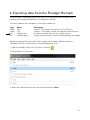
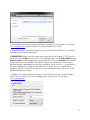
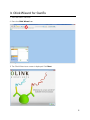
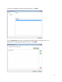
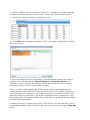
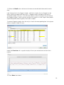
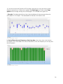
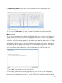
Olink Wizard for GenEx
USER GUIDE
Version 1.1 (Feb 2014)
TECHNICAL SUPPORT
For support and technical information, please contact [email protected], or join the GenEx
online forum: www.multid.se/forum.php.
Table of contents
1.
INTRODUCTION………………………………………………… ……… 4
2.
EXPORTING DATA FROM THE FLUIDIGM BIOMARK………………………..
3.
OLINK WIZARD FOR GENEX……………………………………………… 8
4.
NORMALIZATION METHOD………………………………………………
5.
LINEAR VALUES………………………………………………… ……… 16
5
15
3
1. Introduction
The Olink Wizard add-on feature for GenEx is an easy-to-use data import and
pre-processing tool. The Wizard will guide you through all steps of importing
data, validating data quality and normalization of your Proseek Multiplex data,
preparing it for statistical analysis with the GenEx software.
In short:
►Export your data from the Fluidigm® BioMark
►Follow the Olink Wizard for GenEx for quality control and normalization of
your data
►Continue with statistical analysis of your data, such as hierarchical clustering
methods, principal component analysis and more using the GenEx software.
4
2. Exporting data from the Fluidigm Biomark
The result from a Proseek® Multiplex run consists of two folders and a number of files
created by the Fluidigm® BioMarkTM Data Collection software.
The most important files and folders in the chip run folder are:
Type
Folder
Folder
File
File
Name
Data
Cals
ChipRun.bml
ChipRunLog.txt
Description
Contains TIFF-images, used to extract RT-qPCR data
Contains TIFF-images, used to set exposure times and focus
File containing data from the run, used for analysis
Log file over the chip run, used for troubleshooting and support
Before starting the Olink Wizard for GenEx, export your Fluidigm ChipRun.bml file as a
HeatMap result file in the file format comma separated file (.csv):
1. Open the Fluidigm Real-Time PCR Analysis software (
).
2. Select Open in the File menu.
3. Select the ChipRun.bml file you want to analyze and click Open.
5
4. Add sample information using Sample Setup according to manufacturer’s instruction
(www.fluidigm.com). Sample names can also be altered later in GenEx.
5. Biomarker names are inserted automatically in the Olink Wizard for GenEx, so there is
no need to add Detector information.
6. IMPORTANT! Make sure that the baseline correction in the Fluidigm RT-PCR Analysis
Software is set to Linear and that the Ct Threshold Method is set to Auto (Global) under
Analysis views. When changing this setting you need to click the Analyze button before
exporting the data. Auto (Global) Threshold is used to avoid differences in dCq values
between proteins depending on where the threshold is set for each run. It is possible to
use other methods for setting the threshold, but this might result in samples being
flagged as outliers in the Wizard. Keep this in mind when comparing several runs if you
decide to change this setting.
7. Optional: For a quick overview of the data, use the built in functions of the Fluidigm
Real-Time PCR Analysis software according to the manufacturer’s instructions
(www.fluidigm.com).
6
8. Select Export in the File menu to export your data.
9. Name your data file in the File name box.
10. Select Heat Map Results (*.csv) in the Save as type menu.
11. Click Save. The exported ChipRun_HeatMap.csv file can now be used for analysis with
the GenEx software.
7
3. Olink Wizard for GenEx
1. Start the GenEx software.
2. Press the Olink Wizard icon.
3. The Olink Wizard start screen is displayed. Click Next.
8
4. Select the appropriate Proseek Multiplex panel. Click Next.
5. Press Select files and select the exported Fluidigm BioMark HeatMap files (.csv).
Multiple files can be selected for batch analysis. Click Next.
9
6. You are now on the Sample Plate layout page where you can adjust the sample names
and define Negative and Interplate Controls (IPC). IPC is an additional control that
compensates for possible variations between runs. Negative controls are used to
calculate the detection limit (LOD). LOD is defined as the mean value of the negative
controls + 3 calculated standard deviations (calculated from large sets of data analyzed
by Olink). Measurements below LOD would compromise statistical analysis and are
therefore replaced by “NaN” (not a number) or the LOD value.
If you have used the standard Olink Plate Layout as defined by Figure 2 in the Proseek
Multiplex User Manual, the samples will be labeled as shown in the image below. You
can also paste sample names from an Excel spreadsheet or enter them manually.
7. If you have used your own layout you need to change the setup and place the negative
controls and IPC in the correct position. Do this by right-clicking on the cell that you want
to re-define and choose either “negative control”, “IPC” or “sample”. You can also
choose to exclude some cells from the analysis by selecting “not used”. A minimum of
one negative control is needed to estimate the background level, but it is strongly
recommended that you use at least three negative controls as well as three IPCs.
Selected negative controls and IPCs are indicated with different colors as seen in the
figure below.
8. You can at any time press the View data button to see the data in a new window, the
Data Editor. In the Data Editor you can follow changes made to the data set throughout
the different steps in the wizard. In the Data Editor you can also edit the data manually
and get an overview of the data.
10
9. If several ChipRun files are analyzed in a batch, IPC and Negative Controls should be
included and defined separately for each chip. Change chip in the drop down menu.
10. Press Next when all Negative Controls and IPC’s have been selected for all ChipRun
files in the analysis.
11. Now you are on the Quality Control page. Proseek Multiplex contains four internal
controls; two Incubation controls, Extension Control and Detection Control. The
Extension Control is used for normalization and the other three controls are used to
evaluate the quality of the run and individual samples.
Firstly, a sample will be flagged if one of the internal controls (corresponding to that
sample) deviates more than 0.3 NPX from the median value in all samples. Secondly, to
assess the quality of the entire run, the standard deviations of Incubation Control 2 and
Detection Control are calculated. If any of the standard deviations are higher than a predetermined quality threshold (included in the wizard) they are considered too high and the
run might need to be redone.
A separate summary is shown for each chip. Missing data (Cq values above 30, which is
considered unreliable) will be indicated in red. You can view this by clicking the View data
button.
11
12. Select the Details tab in the lower left corner to see detailed information for each
chip.
Look through the list for flagged samples. Individual samples that are flagged can be
either used or excluded from the analysis. Flagged samples included in the analysis
should be handled with care. A Classification column in the final output file will indicate
the flagged samples, which facilitates removal of samples at a later stage if their protein
expression profiles deviate greatly from other samples.
To remove flagged samples from the analysis check the corresponding box in the Ignore
column and press Redo QC tests.
Under the Overview tab is a graphic display of how your controls deviate from their
median.
13. Press Next when done.
12
14. You are now on the Overview of Data page. Here you can view your data in three
different control charts. Select chart type on the Chart type tab. Switch to the Page
options tab to change settings or to scroll pages. The available chart types are:
a. Box plot: Each box-and-whisker shows the distribution of the measured values for
each protein in all samples. The red dotted line indicates the median value.
b. Limit of Detection and frequency of missing data: A bar chart shows the fraction
of samples with values below the Limit of Detection (LOD) and frequency of missing data
for each protein.
13
c. Sample value profiles: Profile plots show variation of the measured sample values
for the selected proteins.
15. You can click View data at any time to inspect the individual data in the Data Editor
and determine whether any sample or protein needs to be removed from the analysis. Press
Next to proceed.
16. You are now on the final page of the Olink Wizard where you can replace missing data and
sample value data below LOD with the corresponding LOD value. This serves two purposes.
Firstly, it reduces the risk that values below LOD affect the statistical analysis. Secondly, many
multivariate statistical methods require full sets of data and cannot be used on data sets where
values are missing. If you select No Action you can handle missing data later in the GenEx
data editor or limit the analysis to univariate methods that tolerate missing data. Here you can
also choose to convert your data to linear values for further processing, such as calculating the
Coefficient of Variation (CV). You will then get one data sheet with log2 data and one with
linear data. Please note that the GenEx statistical tool works only with log scale data.
17. Press Next. You will now leave the Olink Wizard.
The data import, normalization and quality control in the Olink Wizard are now completed.
Your data set will next be displayed in the Data Editor. There you can perform additional preprocessing steps before statistical analysis, see the GenEx User Guide for further information.
14
4. Normalization method
Cq values from the Fluidigm run are imported into the wizard. The pre-processing steps
convert the imported Cq values (log2 scale where lower values correspond to higher
protein levels) to NPX values (still in log2 scale but now lower values correspond to lower
protein levels).
a) The first two steps performed are normalization against the Extension Control for each
sample, and the Interplate Control corresponding to each protein.
dCqanalyte = Cqanalyte – CqExtension Control
ddCqanalyte = dCqanalyte – dCqIPC
b) In the third step the NPX values are defined by the difference between the calculated
ddCq value and a pre-determined correction factor. The generated NPX will now be in log2
scale where a low value corresponds to low protein levels.
NPX = Correction factor – ddCqanalyte
15
5. Linear values
NPX values are logarithmic. A difference of one NPX unit between two samples
corresponds to approximately twice the amount of protein detected. For manual analysis,
or simply to get an overview of the data, it may be easier to look at linear values. Convert
your NPX values to linear values by using this formula: 2NPX. Coefficient of Variation (CV)
between replicate samples always need to be calculated by using linear values.
16
Olink Bioscience
Dag Hammarskjölds v. 52B
SE-752 37 Uppsala, Sweden
www.olink.com
0964, v.1.1, 2014-02-17
The following trademarks are owned by Olink AB: Olink®, Olink BioscienceTM, and Proseek®.
The following trademarks are owned by MultiD: MultiDTM and GenExTM.
Copyright © 2014 Olink AB.