Download Department of Computing Science and Mathematics University of

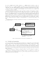
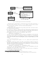
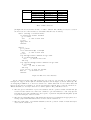
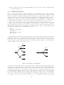
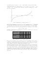
Department of Computing Science and Mathematics
University of Stirling
Extending the model of the Decision Tree
Richard Bland
Department of Computing Science and Mathematics
University of Stirling
Stirling FK9 4LA
Scotland
Claire E Beechey
Department of Computing Science and Mathematics
University of Stirling
Dawn Dowding
Department of Nursing and Midwifery
University of Stirling
Technical Report CSM-162
ISSN 1460-9673
August 2002
Department of Computing Science and Mathematics
University of Stirling
Extending the model of the Decision Tree
Richard Bland
Department of Computing Science and Mathematics
University of Stirling
Stirling FK9 4LA
Scotland
Claire E Beechey
Department of Computing Science and Mathematics
University of Stirling
Dawn Dowding
Department of Nursing and Midwifery
University of Stirling
Department of Computing Science and Mathematics
University of Stirling
Stirling FK9 4LA, Scotland
Telephone +44-786-467421, Facsimile +44-786-464551
Email [email protected]
Technical Report CSM-162
ISSN 1460-9673
August 2002
Contents
Abstract
ii
Acknowledgements
iii
1 Introduction to Decision Trees
1
2 The existing model
4
3 Extending the model
3.1 Adding text . . . . . . . .
3.2 Variables and expressions
3.3 Evaluables . . . . . . . . .
3.4 Macros . . . . . . . . . . .
3.5 Viewing modes . . . . . .
3.6 Question Nodes . . . . . .
3.7 Conditional existence . . .
3.8 Composition of nodes . .
.
.
.
.
.
.
.
.
.
.
.
.
.
.
.
.
.
.
.
.
.
.
.
.
.
.
.
.
.
.
.
.
.
.
.
.
.
.
.
.
.
.
.
.
.
.
.
.
.
.
.
.
.
.
.
.
.
.
.
.
.
.
.
.
.
.
.
.
.
.
.
.
.
.
.
.
.
.
.
.
.
.
.
.
.
.
.
.
.
.
.
.
.
.
.
.
.
.
.
.
.
.
.
.
.
.
.
.
.
.
.
.
.
.
.
.
.
.
.
.
.
.
.
.
.
.
.
.
.
.
.
.
.
.
.
.
.
.
.
.
.
.
.
.
.
.
.
.
.
.
.
.
.
.
.
.
.
.
.
.
.
.
.
.
.
.
.
.
.
.
.
.
.
.
.
.
.
.
.
.
.
.
.
.
.
.
.
.
.
.
.
.
.
.
.
.
.
.
.
.
.
.
.
.
.
.
.
.
.
.
.
.
.
.
.
.
.
.
.
.
.
.
.
.
.
.
.
.
.
.
.
.
.
.
.
.
.
.
.
.
.
.
.
.
.
.
.
.
.
.
.
.
.
.
.
.
.
.
.
.
.
.
.
.
.
.
.
.
.
.
.
.
.
.
.
.
.
.
.
.
.
.
.
.
.
.
.
.
6
6
8
9
11
13
13
19
20
4 Summary and conclusion
24
5 References
26
List of Figures
1
2
3
4
5
6
7
8
9
10
11
12
13
14
15
16
17
18
19
20
21
22
Should we buy shares, or a Government Bond? . . . . . . . . . . . . . . . . . . . . . . . .
The tree with probabilities and payoffs . . . . . . . . . . . . . . . . . . . . . . . . . . . . .
Calculating the tree . . . . . . . . . . . . . . . . . . . . . . . . . . . . . . . . . . . . . . .
Using “utilities” . . . . . . . . . . . . . . . . . . . . . . . . . . . . . . . . . . . . . . . . .
What to do on Sunday afternoon . . . . . . . . . . . . . . . . . . . . . . . . . . . . . . . .
E/R diagram of the conventional Decision Tree . . . . . . . . . . . . . . . . . . . . . . . .
A simple text representation of the Sunday tree . . . . . . . . . . . . . . . . . . . . . . . .
XML representation of the Sunday tree . . . . . . . . . . . . . . . . . . . . . . . . . . . .
UserText in a node . . . . . . . . . . . . . . . . . . . . . . . . . . . . . . . . . . . . . . . .
E/R diagram of Decision Tree with display texts . . . . . . . . . . . . . . . . . . . . . . .
E/R diagram of Decision Tree with variables . . . . . . . . . . . . . . . . . . . . . . . . .
A fragment of a tree, showing QNs . . . . . . . . . . . . . . . . . . . . . . . . . . . . . . .
Specifying a Question Node(QN) . . . . . . . . . . . . . . . . . . . . . . . . . . . . . . . .
The QN of Figure 13 . . . . . . . . . . . . . . . . . . . . . . . . . . . . . . . . . . . . . . .
A Satisfied QN asking its question . . . . . . . . . . . . . . . . . . . . . . . . . . . . . . .
Rule 1 for exit behaviours . . . . . . . . . . . . . . . . . . . . . . . . . . . . . . . . . . . .
Rules 2 & 3 for exit behaviours . . . . . . . . . . . . . . . . . . . . . . . . . . . . . . . . .
Simplification using ExistsIf . . . . . . . . . . . . . . . . . . . . . . . . . . . . . . . . . . .
Nodes that could be composed . . . . . . . . . . . . . . . . . . . . . . . . . . . . . . . . .
Composing Cold and Wet . . . . . . . . . . . . . . . . . . . . . . . . . . . . . . . . . . . .
Transformation of utilities; neutral = 75 . . . . . . . . . . . . . . . . . . . . . . . . . . . .
E/R diagram of Extended Decision Tree . . . . . . . . . . . . . . . . . . . . . . . . . . . .
1
2
2
3
4
5
6
7
7
8
10
14
15
15
16
17
18
19
20
22
23
24
List of Tables
1
2
Exit behaviours . . . . . . . . . . . . . . . . . . . . . . . . . . . . . . . . . . . . . . . . . . 17
Examples of composed utilities; neutral = 75 . . . . . . . . . . . . . . . . . . . . . . . . . 23
i
Abstract
Decision Trees are a familiar tool for the analysis and presentation of problems involving choice between
different possible courses of action. In the conventional Decision Trees there are three types of node (Decision, Choice, and Terminal) and nodes have a small number of possible attributes (name, probability,
and payoff). After a brief introduction to the conventional Decision Tree, this paper presents a series of
extensions of this standard model. The additions greatly extend the expressive power of Decision Trees,
particularly when they are used as a way of conveying information about the context and consequences
of the decisions. The extended model adds a new type of node: the Question node, and a much richer
range of attributes for nodes and for the tree as a whole. This extended model is independent of any
particular (computer) implementation of Decision Trees. It can be used as a way of thinking about the
formal properties of Decision Trees, and as a basis for different implementations.
The extended model has been implemented by the authors, and is being used within a project to
explore the use of Decision Trees as a way of conveying medical information to patients.
ii
Acknowledgements
The work reported here is part of the project The Development and Evaluation of a Computerised Clinical Guidance Tree for Benign Prostatic Hyperplasia and Hypertension, funded by the Chief Scientist’s
Office of the Scottish Executive with a grant for £150K over three-and-a-half years from March 2000.
This project is being undertaken by staff from the Stirling University Department of Nursing and Midwifery (Dawn Dowding, Audrey Morrison, Anne Taylor, and Pat Thomson), Forth Valley Primary Care
Research Group (Chris Mair and Richard Simpson), Department of Psychology (Vivien Swanson), and
Department of Computing Science & Mathematics (Claire Beechey and Richard Bland).
iii
1
Introduction to Decision Trees
Almost every situation in human affairs involves choices between alternative courses of action. A Decision
Tree is a standard way of displaying the choices that can be made in a given situation, together with the
possible outcomes of those choices. They allow the exploration of normative models based on expected
utilities. For discussions of Decision Trees, see [4], [5], [1], and [13].
For example, suppose that we have £1,000 to invest for a year 1 , and are considering two possibilities:
a Government Bond that will yield a guaranteed return (say 3%) and the shares of a pharmaceutical
company that is developing a new product: a treatment for male pattern baldness, say. If the product
succeeds in the next year, the shares will go up in value: otherwise, they will fall. We suppose that we
have estimates of the probability of success and of the possible changes in the share price. (We shall also
assume, to begin with, that we can afford to lose the money.)
Figure 1 shows how this could be represented as a Decision Tree. The tree is made up of three kinds
of node, connected by branching lines. The name or label of each node is shown on the line leading up
to the node. At the right-hand-side of the tree we have Terminal nodes, shown as small vertical bars.
These represent the various final outcomes. We also have a Decision node, shown as a square. This is
a branching point at which a decision can be made: do we buy the share, or the Government Bond?
Finally, there is a Chance node, shown as a dot. This is also a branching point, but it is one where fate,
chance, or other outside agency, determine the outcome: we ourselves are unable to influence whether
the treatment will be a commercial success.
Figure 1: Should we buy shares, or a Government Bond?
The leftmost node in the tree is the root node. Nodes that are connected by lines are parent (to
the left) and child (to the right). The children of the same parent are called siblings. If we trace lines
backwards (to the left) from any child node we go though the ancestors of the node, all the way back to
the root. Obviously, the root is an ancestor of all the other nodes in the tree.
Associated with the children of a chance node are Probabilities: estimates of the relative likelihood
of the various branches. These must sum to 1.0. For example, suppose that analysts think that there
is a 10% chance that the firm’s new product will be a success, then the probability is 0.1, and the
corresponding probability (that the product will fail) is 0.9. (Of course, the children of a decision node
don’t have probabilities: the choice between the children is under human control and is not a matter of
chance.)
Associated with terminal nodes are Payoffs: the value of that outcome. For example, the payoff
associated with the terminal node “Government Bond” is £30: the amount that our £1,000 would earn
in a year at 3% interest. The payoffs that we would get at the other two nodes are the profit (or
loss) that we would make if the new treatment was successful (and the shares went up) or unsuccessful
(and the shares went down). If we can estimate the likely share prices under the two scenarios, then
we can calculate estimates of these payoffs. Suppose that the current share price is 100 pence, and
analysts reckon that it would rise to 2,000 pence if the treatment were successful: then the payoff at the
“Treatment works” node will be our profit of £19,000. If analysts also reckon that the price would sink
to 5p if the treatment were unsuccessful, then the payoff at the corresponding node is our loss of £950.
The tree with its probabilities and payoffs is shown in Figure 2.
1 The
form of this example is based on an example in the manual for DATA 3.5 by TreeAge Software, Inc [16]
1
Figure 2: The tree with probabilities and payoffs
If we have estimates for all the probabilities associated with chance nodes, and the payoffs associated
with terminal nodes, then we can compute an optimal path through the tree. In effect, we can suggest to
the human user which course of action is likely to give the best outcome. The calculation of the optimal
choice, or set of choices, is done by working backwards through the tree, calculating the values of the
nodes from right to left. The values of the terminals are simply their payoffs. The value of a chance
node is its expected value, which can be calculated from the probabilities and values of its children. For
each child, we multiply the probability and value, and sum the answers. In the case of the example, the
node “Buy the Share” has an expected value that can be calculated from the probabilities and payoffs
of its two children, “ ... treatment works” and “ ... treatment fails”. For each child, we multiply the
probability and payoff, and sum the answers. Using the figures that we already have, and writing P for
probability and V (Value) for payoff, this is
EV = P (Success) × V (Success) + P (F ailure) × V (F ailure)
Using the figures that we established earlier, this is
EV = 0.1 × 19000 + 0.9 × (−950) = 1900 − 855 = 1045
Finally, the value of a decision node is the maximum value of any of its children: we assume that a
human, using the tree as a guide to behaviour, will choose the branch with the largest value. This means
that the value of the root node is the value of the “Buy the share” node, that is, £1045. The results
of these calculations is shown in Figure 3, in which the values of the nodes are shown in superimposed
boxes. We see that the optimal path is to buy the share.
Figure 3: Calculating the tree
In our discussion so far, the payoffs have been simple monetary values. Although our discussion did
not stress this, a crucial assumption lay behind the calculation that the purchase of the share was the
“correct” choice. This was an assumption that the relative monetary values reflected the user’s own
relative values. Our assumption had the same general form as an assumption that the gain of £10 is
twice as desirable as the gain of £5.
2
Although this kind of assumption seems reasonable in this case, it is not automatically true. Perhaps
at the end of the year the investor needs to be able to produce the original £1,000 to pay off a loan.
In this case, the outcome “ ... treatment unsuccessful” would be very serious, because the investor has
lost the money. Here we would wish to allow the user to place his or her own subjective weights on the
outcomes. We shall refer to these subjective weights as “utilities”: the value that a particular outcome
has for some individual user. Suppose that we ask some user to rate our three possible outcomes on a
scale of 0 (worst) to 100 (best), and he or she rates them as follows:
• Buy share, treatment successful (100: ideal)
• Buy share, treatment unsuccessful (0: disaster)
• Buy Government bond (20: tolerable)
- then the tree, when calculated, gives a different result. The best path is to buy the Government bond,
with an expected outcome (in terms of the user’s utilities) of 20. This is shown in Figure 4.
Figure 4: Using “utilities”
By asking users to attach their own utilities to the various outcomes, we can extend the Decision
Tree method to areas where there are no obvious numerical “payoffs”. For example, we can consider
what to do on Sunday afternoon. Here the question is whether we should go out for a walk, or stay at
home to read the Sunday paper. The latter is safe but dull. The success of the walk will depend on the
weather: if it clears up, the walk will be very enjoyable, but less so if it rains.
This is, of course, a decision of just the same form as our previous one. We are contrasting an option
subject to a chance outcome with a safe (but dull) alternative. Naturally, the tree will have the same
shape. The details can be quickly supplied. Suppose we have an estimate of the probability of rain (0.7,
perhaps), and the user supplies utilities such as:
• Walk, weather good(very pleasant: 80)
• Walk, it rains (rather disagreeable: 30)
• Read the paper at home (rather boring really: 40)
- then we end up with the tree shown in Figure 5. Using these figures, the tree suggests that even with
Scottish weather the user should take the risk and go for the walk.
The best way(s) of eliciting utilities from the user, and whether utilities can always be treated as
points on a single scale with a metric, are complex issues that we do not deal with here. There is
an extensive literature that goes back to von Neumann and Morgenstern ([17] and [6]: for a specific
discussion, see [12]).
So far, our discussion has concentrated on the fact that Decision Trees can be used to calculate an
optimal course of action. However, it has been suggested (see [7]) that they can also be used as a way
of conveying information about the range of choices, and the range of possible outcomes, in a given
situation. By browsing in the tree, rather than computing the optimal path, a user may obtain a great
deal of useful information. This may clarify their thoughts about the situation, even independently of
any need to take a decision. It may thus be the case that the user, by browsing the tree, comes to
have a much better informed view of their present situation, and a deeper understanding of it. This
information-presenting role is the focus of a project currently under way at Stirling.
3
Figure 5: What to do on Sunday afternoon
The focus of our work is principally on the information-presenting role of Decision Trees. Decision
Trees in the medical domain have been referred to as “Clinical Guidance Trees” (CGTs): see, for example,
[5]. As the name suggests, CGTs have usually been seen as a tool for the medical professional. Our
emphasis is on their role as a way of informing the patient, enabling them to have a more complete
understanding of the issues involved in their treatment.
The two conditions for which we are developing CGTs were selected in the light of this interest in
informing and involving the patient. Benign Prostatic Hyperplasia (BPH) is a common condition with a
range of possible treatments, some of which have significant side-effects. It is important that the patient
who is considering (say) surgery should have a clear understanding of what these side-effects are, and
their probabilities. Chronic Hypertension (CH), on the other hand, is asymptomatic but potentially
serious, and some drug treatments have unpleasant side-effects: thus in this condition the patient’s
compliance with their treatment (continuing to take the drug(s)) becomes an issue. It seems likely that
a patient who has a fuller understanding of their condition will be more likely to continue with the
recommended treatment.
Although we have been developing trees for these two medical conditions, together with software to
display those trees, we have tried to make our work as broadly applicable as possible. Our aim has been
to develop tools and models that will be general-purpose, and which can be used in a wide variety of
contexts. In particular, we have added a number of features to the conventional Decision Tree. These
features, which greatly increase its expressive power, are described in the rest of this paper.
2
The existing model
In this section and the next we discuss Decision Trees using concepts drawn from Object-Oriented (OO)
analysis (see [14], [15]) . For present purposes this style of analysis has strong resemblances to the EntityRelationship (E/R) analysis used in designing databases (see e.g. [2], [3]). By considering Decision Trees
in this abstract way we can ignore the particular features of existing (or future) computer programs for
displaying trees. We can specify the features that a tree author (normally a subject specialist) would
want to be able to use, and we can specify them in a way that is independent of any particular set of
computing tools. In principle, this would allow us to define ways of actually writing trees in a programindependent way, though of course in practice we would need to be able to transform these trees into
the particular input formats required by particular programs for displaying and manipulating trees. To
make practical use of Decision Trees we shall need at the minimum a program that we can call a Tree
Viewer, which displays trees to the user. It will also be useful to have Authoring tools that will enable
trees to be developed. However, our purpose in these sections is to discuss the conceptual structure of
trees and not how particular representations can be manipulated.
In our analysis we shall identify entities and their attributes. For example, a car is an entity with
attributes such as its make, colour, price, and so on. We shall also discuss relationships between different
entities. For example, we can have an “ownership” relationship between a person and a car. A common
relationship between two entities is simply that one entity contains the other: for example a car is an
entity that contains components such as the engine or the wheels, and we can think of these components
as entities in their own right. The component entities will each have their own attributes: the engine’s
4
attributes will include its cubic capacity, power and so on; the wheels’ attributes will include diameter,
weight, and so on.
We can think of a Decision Tree as an entity. A Decision Tree, of course, contains nodes, and so
we can distinguish these as entities in their own right. In the case of the conventional Decision Tree, a
tree entity has no significant attributes of its own (other than, say, its name), and a node entity has five
attributes. These are as follows.
Label Each node will have some unique text that identifies it: we can call this the label.
Parent Every node, except one, will have a parent. Obviously, the one node without a parent is the
root of the tree. For all other nodes, this attribute will give the parent’s identifying label.
Type The node will have a type. There are three possible types: Decision, Chance, and Terminal.
Probability A node may have a probability, 0 < p < 1. This attribute is only meaningful for the
children of a chance node.
Payoff A node may have a payoff, which will be numeric. This attribute is only meaningful for terminal
nodes.
Figure 6 expresses this structure as an E/R diagram. The diagram shows our two entities, listing their
Tree
Name : text
contains
Node
Label : text
Parent : text
Type : {Decision, Chance, Terminal}
Probability : 0<p<1
Payoff : number
parent of
Figure 6: E/R diagram of the conventional Decision Tree
attributes. The diagram has the following characteristics
• The type of each attribute is indicated after a colon. For example, the label of a node can be any
text, and the type of a node must be one of Decision, Chance, and Terminal.
• The relationship between the entities is expressed by the connecting line labelled “contains”. The
fact that a single tree can contain many nodes is expressed by the “crowsfoot” at the right-hand
end of the connecting line. We can also indicate the “optionality”: that is, whether the relationship
is compulsory or optional. Here the relationship is compulsory. As a result the line is drawn solid
(not dashed), indicating that a tree must have nodes and that a node must belong to a tree.
• The fact that a node may be the parent of one or more other nodes is expressed by the connection
from the node entity back to itself, labelled “parent of”. The connecting line is dashed, because
that a node need not be the parent of any nodes, and one node (the root) will not have a parent.
We can test this analysis by seeing whether existing Decision Trees can be expressed in terms of these
two entities and six attributes. To do so, we can take one of our earlier examples. It is easy to see that
we can use our framework to express (say) the sample tree of Figure 5 as a single tree object containing
five node objects. The objects will have the attributes shown in Figure 6. This re-writing of the tree is
shown in Figure 7.
It is clear that the tree drawn in Figure 5 contains exactly the same information as the tree shown
in text form in Figure 7. The former has the advantage that its structure is more appealing to the
human eye, while the latter has the merit that it illustrates the entity-attribute structure discussed in
the previous paragraphs. The text representation also has the considerable advantage that it can be
manipulated by computer. In fact, at the cost of some textual clutter we can express the tree more
formally using the conventions of the Extensible Markup Language XML (on which, see for example [9]).
This is shown in Figure 8.
5
Sunday walk tree
<node>Sunday Afternoon
<type>Decision
<node>Go for a walk
<parent>Sunday Afternoon
<type>Chance
<node>Pleasant walk
<parent>Go for a walk
<type>Terminal
<probability>0.3
<payoff>80
<node>Wet walk
<parent>Go for a walk
<type>Terminal
<probability>0.7
<payoff>30
<node>Read Sunday papers
<parent>Sunday Afternoon
<type>Terminal
<payoff>40
Figure 7: A simple text representation of the Sunday tree
3
3.1
Extending the model
Adding text
The conventional CGT model, as we have seen, does not allow nodes to have extended texts. A node’s
identifying label is the only possible documenting feature. However, any tree author would want each
node to be able to explain itself to users viewing the tree. To accommodate this we shall need a new
field to contain the explanatory text. In fact we add two further fields to the Node entity. These are the
UserText and DocumentingText fields. The tree author can use the UserText field to give explanatory
material relevant to the node. This will be material that the tree author would expect to be available
to ordinary users who are viewing the tree. An example, using the conventions of XML, is shown in
Figure 9, in which the UserText material is shown in a larger font than the rest of its node.
The DocumentingText field is similar: it too is used to contain text that explains the node. However,
the UserText material is intended to be shown to the ordinary lay user of the tree, while the DocumentingText contains technical notes for the tree author(s) or their peers. For example, it could be used to
give bibliographic and other information about the studies consulted by the author while writing this
part of the tree. This facility to store technical supporting documentation as part of the tree is very
useful. It means that the tree author’s own notes are stored in the most relevant place: next to the
tree structure itself. Obviously, a tree Viewer program implementing our extended model would provide
facilities whereby DocumentingText can be displayed, but also facilities that would allow its display to
be distinguished from UserText, or suppressed entirely.
In the example in Figure 9 the UserText is plain text: it contains no indication as to how the text
is to be displayed. However, it is clear that a tree author would normally want to have some control
over such features as emphasis, paragraph breaks, headings and so on. The author might also wish to
include graphics such as illustrative pictures. These considerations suggest that the for the User and
Documenting texts should allow the author to specify layout features. It would be undesirable for this to
be proprietary. It would, however, be highly desirable that the should be an already existing standard,
based on ordinary (7-bit) ASCII characters. The obvious candidate here is HTML ([8]). Among the
many advantages of HTML we can cite its widespread use, its portability, and the fact that a Viewer
program can use existing code to handle the text. Such code (as a WWW browser) would be already
available on most machines. This would greatly simplify the task of writing a Viewer program. Ideally,
6
<tree>
<name>Sunday walk tree</name>
<node>
<label>Sunday Afternoon</label>
<type>Decision</type>
</node>
<node>
<label>Go for a walk</label>
<parent>Sunday Afternoon</parent>
<type>Chance</type>
</node>
<node>
<label>Pleasant walk</label>
<parent>Go for a walk</parent>
<type>Terminal</type>
<probability>0.3</probability>
<payoff>80</payoff>
</node>
<node>
<label>Wet walk</label>
<parent>Go for a walk</parent>
<type>Terminal</type>
<probability>0.7</probability>
<payoff>30</payoff>
</node>
<node>
<label>Read Sunday papers</label>
<parent>Sunday Afternoon</parent>
<type>Terminal</type>
<payoff>40</payoff>
</node>
</tree>
Figure 8: XML representation of the Sunday tree
<node>
<label>Sunday Afternoon</label>
<type>Decision</type>
<usertext> We are deciding what to do on Sunday
afternoon, and are considering reading the Sunday paper.
However, we are also considering going for a walk.
It is cloudy at present.
</usertext>
</node>
Figure 9: UserText in a node
7
the version of HTML should be XML compliant (i.e. be XHTML). This would make it possible for
the whole of the tree to be handled by XML tools: if this were the case then the Viewer program and
Authoring tools would be further simplified because the data structures and manipulation procedures
could use library code. For flexibility (and anticipating later material) we shall use the term DisplayText
to indicate the data-type of UserText and DocumentingText. For the moment the user can think of this
as meaning some flavour of HTML.
The UserText(s) in the tree are likely to involve specialised vocabulary: medical terms, for example.
We therefore extend the specification of the Tree entity to allow for the tree to contain a Dictionary: a
list of words and phrases, each with an extended explanation (the Definition) attached. The definitions
should be in the DisplayText that we introduced in the last paragraph. Clearly, this implies that any
Viewer program must be capable of recognising Dictionary terms in DisplayText, and modifying the
display so that the user can click the term and see its definition. In fact this should be a feature of any
DisplayText, no matter where it occurs in a tree: when displayed, dictionary terms should be clickable.
This is recursive: a Dictionary Definition can itself contain terms that are in the Dictionary, and they
should be clickable when they are displayed. An implementation of a dictionary will probably be in
XML.
The E/R diagram shown in Figure 10 summarises the changes to the standard Decision Tree that we
have described so far.
Dictionary
Name : text
cites
Tree
Name : text
contains
contains
Dictionary Entry
Term : text
Definition : DisplayText
Node
Label : text
Parent : text
Type : {Decision, Chance, Terminal}
UserText : DisplayText
DocumentingText : DisplayText
Probability : 0<p<1
Payoff : number
parent of
Figure 10: E/R diagram of Decision Tree with display texts
3.2
Variables and expressions
So far, our examples have had probabilities and payoffs that were constant values, quoted literally. Thus
the probability of rain on a Sunday walk was given as 0.7 in the tree in Figure 5. However, a tree author
is likely to want to be able to use a value several times in the same tree, and it is much safer to do this
using a variable. For example, we could set up the variable (say) pRain to have the value 0.7, and write
the variable’s name in the tree at each point where we want to use that value. This would ensure that
all references to the probability of rain would use the same value. Then, if later research showed that
the true value was 0.8, we would just have to make that change at the single point in the tree where the
variable was set up.
Clearly, the introduction of variables is a further extension to the model. There are a number of
ways in which we could make this extension: the simplest, and the one we shall use, is to declare each
variable at tree level. In computing terms, they are “global” variables, visible from any point in the tree
and having the same value at all points.
8
It is commonly the case that a tree author will want to manipulate variables arithmetically. For
example, if we return to the tree in Figure 2 and look at the payoff for “Buy, treatment works” we see
that it is shown as 19000 (the profit that will be made if the shares are bought and the share price
rises according to the scenario in the tree). But it would be very foolish for the author to enter this
value literally. If the underlying values for the share prices were to change, then the tree author would
need to recalculate the payoffs by hand and re-enter them into the tree. This is a very error-prone
procedure. A much better approach is to define variables to hold the underlying values, and then get
the Viewer program that implements the tree to compute the payoffs. In this particular case we could
declare variables like this:
initialInvestment = 1000
shareNow = 100
shareIfYes = 2000
These declarations also give values for the variables: as we shall see in a moment, this is not always
necessary. Variables can acquire their values later.
Having set up these variables, at the node “Buy, treatment works”, we can change the way that the
payoff is specified. Instead of writing some such specification as
<payoff>
19000
</payoff>
we could write
<payoff>
initialInvestment*(shareIfYes/shareNow - 1)
</payoff>
The particular notation is not important. It should, however be clear that the value at the node is being
specified as a formula rather than as a constant. This is an idea that will be familiar from many other
computing tools: spreadsheets, for example. Just like spreadsheets, a user (here, a tree author) will
want to be able to use standard arithmetic operations, probably some common functions (logarithms,
for example), and also conditionals using if and else. To meet this need, we introduce the idea of
an Evaluable Expression (or just Evaluable), that is, a formula (“expression”) that can be worked-out
(“evaluated”) when its value is needed. We do not need to fix the notation here: we only need to note
that
1. We are extending the definition of a node so that the probability and payoff fields, previously of
type number, are now of type Evaluable.
2. Evaluables can contain the usual apparatus of spreadsheet formulas such as ordinary arithmetic
and standard functions.
The E/R diagram shown in Figure 11 summarises the changes to the standard Decision Tree that we
have described so far. In the next section we develop the idea of the Evaluable.
3.3
Evaluables
The previous section introduced the Evaluable expression, using the example of simple arithmetic formulas. Our own implementation supports addition, subtraction, multiplication, division, x y , e x and
log e x, and the use of brackets. The operators have their usual relative priorities. Raising to a power is
evaluated right-to-left, so 2 ^3^2 gives 512 and not 64. These are a minumum set of arithmetic operators:
obviously others could be added.
We shall, however, need more powerful features than just arithmetic, and in this section we extend
the definition of the Evaluable in other directions.
1. An Evaluable can, in addition to representing a numeric expression, also represent a Boolean
expression, i.e. one that evaluates to either true or false. To make this possible we use use the
9
Dictionary
Name : text
Dictionary Entry
Term : text
Definition : DisplayText
contains
cites
Tree
Name : text
contains
defines
Variable
Name : text
Value : Evaluable
Node
Label : text
Parent : text
Type : {Decision, Chance, Terminal}
UserText : DisplayText
DocumentingText : DisplayText
Probability : Evaluable
Payoff : Evaluable
parent of
Figure 11: E/R diagram of Decision Tree with variables
convenient (if crude) convention that zero represents false and any other value represents true
We can now add the relational operators (> >= < <=), the equality operators (== and !=), and the
logical operators (and, or, and not) 3 . We can now write such expressions as
male and age > 15
(assuming we have declared variables male and age). This expression will be true if male is non-zero
(i.e. true) and age is greater than 15.
2. For convenience, we define two constants, true and false. The first has some arbitrary fixed nonzero value, and the second has the fixed value zero. The user cannot define variables with these
names, and the names cannot be used on the left-hand side of an assignment.
3. The assignment operator (=) can be part of an Evaluable. Thus, in the line
annualSalary = monthlySalary * 12
the whole of the line is an Evaluable expression. The value of an assignment operator is the value
that was placed in the variable on the left-hand side. Thus in the example above, if monthlySalary
has the value (say) 1,500 then the value 18,000 is placed in the variable annualSalary, and 18,000
is the value of the whole expression. The assignment operator is evaluated right-to-left, so the
Evaluable
i = j = k = l = m = n = 0
has the effect of setting the all the variables i to n to zero. (And the whole expression has the
value zero.)
4. An Evaluable expression can consist of more than one sub-expression, separated by semicolons.
The value of the whole Evaluable is the value of the last sub-expression: the rest are discarded.
Although only the last sub-expression gives the value of the Evaluable, the others may have useful
effects. So, for example, in the following Evaluable
annualSalary = monthlySalary * 12 ; annualSalary > 30000
we set the value of the variable annualSalary and test it: the value of the Evaluable is true if the
annual salary is greater than 30,000, and false otherwise.
5. An Evaluable can contain an if-expression. There are two forms: in the notation of our implementation, the syntax of an if-expression is either
IF expression-1 THEN expression-2 FI
or
2 This
is of course the convention in the language C and its derivatives, such as C++ and Perl.
other notations could be used for these operators: we show the notation of our own implementation.
3 Obviously,
10
2
.
IF expression-1 THEN expression-2 ELSE expression-3 FI
In both forms, if expression-1 evaluates to true, then expression-2 is evaluated and its value is the
value of the if-expression. If expression-1 evaluates to false, then in the first form expression-3
is evaluated and its value is the value of the if-expression; in the first form, nothing is evaluated
and the if-expression has no value.
These syntax rules allow an author to use a variety of styles of programming. For example, suppose
that we have a variable age and wish to create a derived variable ageCategory. This is to have the
value 1 for people below 20, 2 for 20 to 39, and 3 otherwise. Here are two ways of expressing this:
the author can user whichever they find clearer and easier to write.
IF age < 20 THEN
ageCategory = 1
ELSE IF age < 40
ageCategory = 2
ELSE
ageCategory = 3
FI FI
ageCategory =
IF age < 20 THEN 1
ELSE IF age < 40 THEN 2
ELSE 3 FI FI
In the style on the left, the expressions inside the IFs are written as assignments. These could
be sequences of assignments. Suppose we have two probabilities, p1 and p2, that should have
different values for the age categories. We could write this as follows (taking arbitrary values for
the probabilities):
IF age < 20 THEN
ageCategory = 1 ; p1 = 0.2 ; p2 = 0.15
ELSE IF age < 40
ageCategory = 2 ; p1 = 0.3 ; p2 = 0.45
ELSE
ageCategory = 3 ; p1 = 0.5 ; p2 = 0.55
FI FI
6. A variable that has been declared but not given a value is undefined. This does not mean that
it has some special numeric value. It means that it does not have a numeric value at all. Any
operation, except one, on an undefined value yields an undefined value. So if y is undefined then
y+2 is undefined, and y==0 is undefined (and not false, surprisingly). The single exception is the
Boolean function defined: thus defined(y) is either true or false. For convenience, we define the
constant, undefined. This constant is (of course) undefined. There is only one useful thing that
can be done with this: to assign it to a variable, thus:
y = undefined
This has the effect of making y undefined. Note that the Boolean expression y == undefined will
always give the undefined value, whether y is defined or not, so this will not test the value of y.
The only possible way of seeing if y is undefined is to use the defined function, as shown earlier in
this paragraph.
If the condition part of an if (the expression-1) is undefined, a run-time error message is generated.
3.4
Macros
It is often the case that a tree author will wish to make use of some standard form of words at a number of
different places in the tree. Suppose, for example, that every time a probability is quoted in a user text,
it is to be explained, as in “the probability of this is about 0.2, or 20 cases in 100” or “the probability
of this is about 0.05, or 5 cases in 100.” Writing these standard forms is tiresome and error-prone: it is
hard to maintain a consistent style, particularly if more than one author is involved, or if it is decided
to adopt a different style.
In addition, a tree author is very likely to want to use the values of tree variables in the text.
Developing the example in the previous paragraph, suppose that there is a tree variable pEvent that
currently has the value 0.2. The tree author could write “the probability of this is about 0.2,” but if the
11
value of pEvent were to change, then the text as it stands would be wrong. It would be far better if the
author had some method of instructing the Viewer program to insert the current value of the variable
in the text.
Our Viewer program meets both of these needs (recurring phrases, and dynamic use of tree variables),
by the use of Macroprocessing. Our approach is based on the Unix macroprocessor m4 4 . A full account
would be out of place here, but our method allows the tree author to define Macros that expand into
standard forms, manipulating and displaying tree variables as they are expanded. It is important to
be clear that these expansions and manipulations do not happen statically as the tree is written, or as
the tree is being read in, but take place dynamically, as the text is being displayed. Thus the the same
fragment of User text will be displayed differently to different users.
Let us look at some examples. First, suppose the tree author defines a macro at the top of the tree
file
McDefine(MildAUA, ‘AUA symptom index 0-7 points’)
Then every time the tree author writes, for example
For MildAUA the likely outcome is ...
the program will display
For AUA symptom index 0-7 points the likely outcome is ...
As a second example, let us take the display of the pEvent variable mentioned above. Using macroprocessing, the tree author simply replaces
the probability of this is about 0.2
by the following
the probability of this is about McEval(pEvent)
and every time the program displays this, it will substitute the correct current value of pEvent.
Now a more elaborate example. Suppose there is a tree variable SymptomScore that holds the current
user’s score in terms of some index (we shall see later how this can be done). If the following macro is
defined at the top of the tree file,
McDefine(SaySymptoms,‘McIfElse(McEval(SymptomScore<8),1.0,mild,
McEval(SymptomScore>20),1.0,severe, moderate) symptoms’)
Then the tree author can write such User text as
Your symptom score is McEval(SymptomScore).
This means that you have SaySymptoms.
and the program will convert this to a text that is tailored to the user. If, for example, the user’s
symptom score is 15, then the program will output
Your symptom score is 15.
This means that you have moderate symptoms.
Macroprocessing gives tree authors a very powerful and flexible tool for writing dynamic user texts.
In effect, it allows them to write small customised text-manipulation programs. Because these textmanipulation programs are contained in the tree file, the whole process is completely under the control
of the tree author(s), and is another powerful aid to customising the Decision Tree display methods for
a particular application.
Formally, macroprocessing represents an extension of DisplayText, the data-type which we introduced
earlier. As we have seen, the extensions are:
4 Developed
by BM Kernighan and DM Richie. See [10] and [11].
12
1. When DisplayText is being displayed, it is scanned for terms that have been defined as macros. The
term is replaced by the macro’s replacement text. This, in the example above the term “MildAUA”
would be replaced by “AUA symptom index 0-7 points”.
2. The scan for macros is recursive: that is, the replacement text itself is scanned for macros.
3. A Viewer program should implement (at least) three built-in macros:
• A macro for defining new macros. This macro itself produces no replacement text. In our
program, this macro is McDefine, as in the examples above.
• A macro with a condition and a choice of replacement texts. The condition determines which
of the various possible replacement texts is used. In our program, this macro is McIfElse.
• A macro that evaluates an Evaluable (Section 3.2, above). The replacement text is (a character
representation of) the number that results from the evaluation. In our program, this macro
is McEval.
3.5
Viewing modes
In the previous section we discussed how the display of texts can be generated dynamically to fit the
characteristics of a particular user. In the next section we discuss one of our major extensions to the
Decision Tree model - a method for querying the user as he or she browses the tree, in order to establish
that user’s characteristics, thus providing the context for text generation. Before we discuss this, a word
about viewing modes.
Our method presumes that the Viewer program offers a viewing mode in which the user scans the
tree’s nodes starting at the root and moving towards the terminal nodes. The critical feature of such
a viewing mode is that there is always a “current node”: the node that the user has just reached.
Obviously, the Viewer program should supply navigational methods that allow the user to move about
the tree: for example, to move to one of the current node’s childen. As a result of any move the “current
node” is the one to which the user has just moved.
We call this mode “Walk-a-Tree” mode (WaT). It is particularly appropriate when the user is reading
the tree in detail, exploring the texts that are attached to each node. A Viewer program will probably
offer other modes: for example a mode in which the user can view all of the tree, both nodes and branches
(or as much of it as will fit on the screen). We call this latter mode “Show-a-Tree” mode (SaT). Such a
mode is appropriate when the user wants to review the overall structure of the tree, in particular when
calculating the optimal path. The crucial difference is that the SaT mode has different navigational
methods: the user will simply scroll the window to see particular parts of the tree that are currently out
of sight. In particular, there need not be a “current node”.
3.6
Question Nodes
As we have seen, to provide customised texts we need to be able to discover the characteristics of each
individual user. As we shall see later, this can also be used to custome the structure of the tree itself.
In designing our method of eliciting user characteristics, we wanted to preserve our major design
goal: the tree author should control the flow of the user’s interaction with the tree, and should exercise
that control by specifications in the tree file. Our method uses a new type of node, which we call the
Question Node. (This node is represented by a diamond shape in our decision trees.)
The tree author specifies QNs in the same general way as any other node type: by indicating which
node is the QN’s parent, and giving a series of node fields. The user will encounter the QNs during an
exploration of a tree in WaT mode (as defined in Section 3.5, above). At that point the QN will ask its
question. In other viewing modes (such as SaT), on the other hand, QNs will be invisible: the user will
simply see a conventional Decision Tree.
These considerations give rise to the following structural rules:
• A QN can be the child of any type of node other than a Terminal
• A QN can be the parent of any type of node, and can have any number of children, subject to the
next rule:
13
• Among the child branches of a QN, no more than one may contain a non-QN node. Another way of
saying the same thing is this: if we take any (sub)tree rooted at a QN and remove every QN from
that (sub)tree (including the root QN itself), the result must either be a single tree or nothing.
These structural principles are illustrated in Figure 12, in which we see two Decison nodes (D1 and
D2) and four QNs (Q1 to Q4). We suppose that this is a fragment of a larger tree, with D1 having some
parent and D2 having at least one child. The significant points are:
• Outside the WaT viewing mode, D2 will appear to be the child of D1 (because QNs are only visible
in WaT mode)
• None of the QNs has more than one non-QN in its child branches: Q1 has one, and Q2 to Q4 have
no children at all.
• As a consequence, if we take the (sub)tree(s) rooted at any of these QNs and remove all QNs, we
either end up with a single tree or nothing. In the case of Q1, we end up with the single tree rooted
at D2. In the cases of Q2 to Q4, we end up with nothing.
We shall return to Figure 12 once we have discussed the entry and exit behaviour of QNs. This material
is covered later in this section.
Q4
Q3
Q2
D1
Q1
D2
Figure 12: A fragment of a tree, showing QNs
Figure 13 gives an example of a QN, expressed in the notation of our program, and Figure 14 shows
how this node would appear on the screen in our implementation. Note that the display of the node
provides a button that the user can use if they wish to skip the question. Because this QN has a child
that is also a QN, the display provides a “Skip all questions” button.
We expect that a Viewer program will offer a number of question formats: the QN in Figures 13
and 14 uses radio buttons to capture the user’s response. In our own implementation, other possible
formats include drop-down lists (a combo-box) and user-entry into a text box.
Every QN is bound to a variable: that is, the user’s response is stored in that variable. In the case of
the QN in Figure 13, it is bound to the variable SexualFunction, which will have the value 0 if the user
selected the “No” button, and 1 if the user selected “Yes”. For a combo-box, the variable will store a
number corresponding to the option, 1 for the first option, 2 for the second, and so on. For a text box,
the variable will store the number entered by the variable in the text box.
A QN’s behaviour is different if it is revisited by the user. In this case it tells the user what he or
she answered last time, and asks if they wish to change their response.
QNs have a ValidationRule field. This can be used by the author to specify a test that the user’s
input should pass. For example, if the Bound variable was Age and the author knew that all users of
the tree should be over 15, the author could specify the rule Age > 15 . If the test fails, then the Viewer
program will display an error message. The author would not normally need to test values being returned
from radio buttons or combo-boxes, because in these cases the values that can be entered are already
controlled.
As another example, the Benign Prostatic Hyperplasia tree asks seven questions about urinary function, and then computes the American Urological Association (AUA) symptom score. In the tree file
these seven questions are written as seven QNs. The seven questions each return a value from 1 to 6
14
ID: Q1
ShortLabel: Your Symptom Score
ParentID: Root
Type: Question
QuestionText: Q1: Over the past month, how often
have you had the sensation of not emptying your
bladder completely after you finished urinating?
InputType: AnsCombo
BoundVariable: AUA1
UserText:
{Question One|One of the most common symptoms of
BPH is the feeling that you haven’t completely
managed to empty your bladder, even though you
have finished going to the toilet.
<p>This question is asking you to think about
how many times on average you have had this
feeling over the last month.}
InstructionText: Select your answer from the drop down
list, then click OK.
Figure 13: Specifying a Question Node(QN)
Figure 14: The QN of Figure 13
15
using combo-boxes, and are bound to the variables AUA1 to AUA7. The validation rule for the final QN
can then be written
SymptomScore = AUA1 + AUA2 + AUA3 + AUA4
+ AUA5 + AUA6 + AUA7 - 7 ;
true
thus computing a SymptomScore ranging from 0 to 35. The final true is just a placeholder to ensure
that the Validation rule “succeeds”: the useful work is done by the assignment that comes before the
semicolon.
We need to be precise about what happens when a user moves to a QN, and about what happens
next, after the user has answered the question (or not: the user may leave the node by clicking the “skip”
button). We talk about the entry behaviour and exit behaviour respectively.
Entry behaviour depends on whether the node is satisfied or not: that is, whether it has received an
answer to its question. When a Viewer program starts to process a tree, all the QNs are unsatisfied :
when a particular node has asked its question and received a valid answer, it becomes satisfied.
On entry, an unsatisfied QN asks its question directly, as in Figure 14. However, a satisfied QN
prompts the user with the last answer, and asks the user if they wish to keep that answer or change
it. This is illustrated in Figure 15.
Figure 15: A Satisfied QN asking its question
Exit behaviour has two aspects: firstly, whether the current node becomes satisfied or not; and,
secondly, which node becomes the new current node. These depend on what the user has entered
(or clicked) at the QN. The possible outcomes are described in Table 1. The rules used to find
the next node are given in Figures 16 and 17. The rules are stated in pseudocode: comments
are introduced by two slashes (like this: // this is a comment). Although these rules seems
complex, their aim is to allow the user to take navigation for granted: when a user leaves a node,
they should find themselves at the node which seems intuitively to be “next”.
16
Node was
Unsatisfied
Satisfied
User does
Valid response
Invalid response
Clicks “Skip”
Clicks “Skip All”
Clicks “Change”
Clicks “Keep”
Node becomes
Satisfied
Unsatisfied
Unsatisfied
Unsatisfied
Unsatisfied
Satisfied
Next node
Rule 1
Current
Rule 2
Rule 3
Current
Rule 1
Table 1: Exit behaviours
(In Figures 16 and 17, mention is made of “visible” children. The visibility of nodes is covered in
the next section: for the moment, we can assume that all nodes are visible.)
Rule 1 (leaving a satisfied node):
if current has visible children
go to eldest
exit
// this is next node
// else
apply Rule 1a
end-rule
Rule 1a :
go to parent
if is unsatisfied QN, or non-QN
exit
// this is next node
// else
loop through visible children in age order
if is unsatisfied QN
exit
// this is next node
end-loop
loop (again) through visible children in age order
if is non-QN
exit
// this is next node
end-loop
// no success, go back one further
Rule 1a
// recursive call
end-rule
Figure 16: Rule 1 for exit behaviours
Let us consider how these rules will work in the case of the set of nodes that we looked at earlier,
in Figure 12. Suppose all the QNs are unsatisfied (indicated in the Figure by hollow diamonds). We
are navigating in WaT mode, so there is a current node: assume this is D1. Let us consider what will
happen as the user moves further on. As the user navigates onwards, Q1 becomes the current node.
This is unsatisfied, so its entry behaviour is to ask its question. The possibilities now are:
1. The user gives a valid answer. Q1 becomes satisfied, and the operation of Rule 1 means that Q2
is entered as the current node. If the user continues to give valid answers, to each of Q2, Q3 and
Q4, then the user will eventually leave the sequence of questions and (still following Rule 1) will
re-join the main part of the tree at D2.
2. The user gives an invalid answer. (We assume that the Viewer program issues an appropriate error
message.) Q1 remains unsatisfied, and is re-entered as the current node.
3. The user clicks “Skip”. Q1 remains unsatisfied, and the operation of Rule 2 means that Q2 is
entered as the current node.
17
Rule 2 (single skip):
loop through visible children in age order
if is node we’re skipping
ignore it
else
exit
// this is next node
end-loop
// no success, go back one
go to parent
if is not a satisfied QN
exit
// this is next node
// else
Rule 2
// recursive call
end-rule
Rule 3 (skip a run of questions):
loop through visible children in age order
if is non-QN
exit
// this is next node
end-loop
// no success, go back one
go to parent
if is non-QN
exit
// this is next node
// else
Rule 2
// recursive call
end-rule
Figure 17: Rules 2 & 3 for exit behaviours
18
4. The user clicks “Skip All”. Q1 remains unsatisfied, and the operation of Rule 3 means that D2
becomes the current node.
3.7
Conditional existence
We have seen that QNs give tree authors the ability to obtain information from the user. The values
are stored in variables: using the facilities of Evaluables we can test the values of variables, modify
them, and compute new variables. We saw in the previous section, for example, how a sequence of seven
questions can be used to compute the American Urological Association (AUA) symptom score. We now
build upon these facilities to provide a feature that allows the tree to dynamically reconfigure itself.
This is achieved by using a new (optional) node field, ExistsIf. In this field, the tree author writes
an expression that will evaluate to true or false using the methods discussed above in Section 3.3.
Suppose, for example, that there are three possible treatments for a condition: call these T1, T2, and
T3. These would be represented by three Chance nodes, the children of a Decision node: call this D1.
Suppose further that T1 would not be offered to a patient who was a sufferer from (say) diabetes, and
that we have a variable diabetic. A QN has already set this variable to be true or false. In the notation
of our Viewer program, the node for T1 could be coded as
ID: T1
ShortLabel: Treatment 1
ParentID: D1
ExistsIf: not diabetic
Type: Chance
...
The right-hand side of Figure 18 shows the structure of this example. The Question node Q1 asks the
question about diabetes (or, perhaps, that question may have been asked earlier); the Decision node D1
presents the choice between the the three treatments; and the nodes T1 to T3 are the roots of the various
possible outcomes of the treatments, which are not shown in the diagram. The node T1 is marked with
a question-mark to indicate that it may not exist.
T1
D1
T2
T1?
T3
Q1
D0
D1
T2
T3
T2’
D1’
T3’
Figure 18: Simplification using ExistsIf
In the basic Decision Tree model, our problem would be represented in the struction shown on the
left-hand side of Figure 18. Here, the Decision node D0 represents the different paths taken for the
non-diabetic (upper branch) and the diabetic (lower branch). The choice between the treatments is
represented as D1, the choice for non-diabetics, and D1’, the choice for diabetics. Because the choice
between the treatments is represented twice, the texts for that choice must be repeated (or partitioned)
in a way that will be awkward for the tree author. The situation becomes worse: two of the treatments
appear twice, as T2 & T2’ and T3 & T3’. The author once again has to include texts twice. If a text has
to be changed to keep the tree up to date, it may have to be to be changed in several places, and perhaps
19
one of them will be forgotten. For the author, the tree becomes difficult to manage, and it is likely that
mistakes will be made. If the tree is viewed by patients, they are very likely to stray into branches of
the tree that are inappropriate.
Using ExistsIf, on the other hand, matters are easier for both the author and the user. The structure
is simpler and clearer. The author needs only write one copy of the various nodes, making the tree easier
to write and to maintain. The only apparent complication for the tree author is that the probabilities
in the treatments’ child nodes will have to be written as expressions involving the variable diabetic,
but in fact this is clearer and easier than remembering that (for example) the children of T3’ must have
probabilities appropriate to diabetics whereas those of T3 must not.
For the user, the ExistsIf mechanism represents a remarkable simplification. The user will see only
the information that is relevant to their circumstances. They cannot stray into irrelevant portions of
the tree because these are literally invisible to them. The user sees a version of the tree that has been
dynamically selected to fit his or her circumstances. This is a very powerful facility.
3.8
Composition of nodes
In this section we describe a way of simplifying the treatment of Terminal nodes. The method is used
where there are a number of independent events that can co-occur to make up an outcome. For example,
consider the fragments shown in Figure 19. At D1 we have the decision whether to go for a country walk
OK
Walk
Walk
Cold
Wet
D1
D1
Cold & Wet
OK
Cold
Tired
Wet
Cold & Tired
Cold & Wet
Tired & Wet
Cold & Tired & Wet
No Walk
No Walk
Figure 19: Nodes that could be composed
or not. The upper branch, a Chance node, deals with the possible outcomes. In the left-hand fragment
we see that the walk may be “OK”, or the walker may get cold, or wet, or both. In essence, there were
two events that might occur, and the possible outcomes are derived by taking the possible combinations.
The general form is this: if we have n events that are not mutually exclusive, then there are 2
possible combinations. Thus if the walker might have got tired as well, there would have been eight
(2 3 ) possible outcomes, and thus eight Terminal nodes. This is shown in the right-hand fragment in
Figure 19. Obviously, the number of terminal nodes can become very large.
Clearly this combinatorial explosion can give problems to both the tree author and the user of the
tree. Consider first the tree author. Even in the three-event case of Cold, Tired, and Wet, any one
event, such as Cold, occurs four times. This means that any Documenting Text (Sections 3.1 and 3.4)
relating to Cold will have to be repeated four times, and the same will apply to Tired and to Wet. As
we saw in the preceding section, this makes the tree hard to write and very hard to maintain. It is all
too easy for the various descriptions to become inconsistent. A second problem for the tree author is
that probabilities must be assigned to each of a large number of nodes, and it may be difficult to find
good estimates in the substantive literature of the domain being modelled in the tree. We may know
the separate probabilities of being wet or cold, but it may be difficult to estimate the probabililty of the
joint event.
Turning to the tree user, they are very likely to be daunted and confused by the large number of
branches that they are offered. This confusion will be made worse by the fact that the nodes will contain
repeated material. The user is likely to lose track of whether they have looked at some particular node
before. A further problem for the user will be the number of utilities that they have to supply. As we
saw in Section 1, to compute the user’s optimal path the software has to obtain the user’s individual
20
n
evaluations of the various outcomes: the “utility” that each outcome has from his or her own perspective.
How this is done is an implementation-specific matter (our implementation invites the user to position
each outcome on an analogue scale) but, however it is done, if there are a large number of outcomes then
the task will become very tedious for the user. If those outcomes contain repeated words or phrases, as
here, the user may be reluctant to complete the task.
In summary, then, the combinatorial explosion brings the following problems:
1. The user has too many nodes to view comfortably.
2. The author has to repeat DisplayText at different nodes.
3. The user has too many utilities to supply without fatigue.
4. The author has to supply a large number of probabilities.
Our method for addressing the combinatorial explosion is the composed node. In our implementation
it solves three of the four problems listed above, and in principle can be extended to solve all four. The
tree author indicates that a particular outcome is “composed” of two or more other outcomes. How this
is done is implementation-specific: in our implementation this is done via the label field of the node.
Thus if we have two “composing” nodes labelled respectively Cold and Wet, then the author gives the
composed node the label [Cold][Wet]. Although the author still has to write a node for every possible
outcome, the material at the composed node can be greatly reduced, as we shall see.
Notice that the tree author does not need to supply a node (whether composed or not) for every
combination that is mathematically possible: only for those that actually occur. Further, the author can
use a mixture of composition and writing a node normally: thus, in the example on the right-hand side
of Figure 19, the author can code some of the combinations as composed nodes and others as normal
Terminal nodes.
The properties of composed and composing nodes are:
1. A composed node is only visible to the user when viewing the optimal path. It is hidden in other
viewing modes, such as Walk-a-Tree mode (WaT). This solves the first of our problems, above: the
user now sees a much simpler structure. In the right-hand tree of Figure 19, for example, there are
now only four visible outcomes of Walk instead of eight.
2. When the user views a composing node in WaT mode, the viewing program automatically appends
a note to the DisplayText to indicate that the event can co-occur with other specific event(s), and
the DisplayText of that event is available. So if we have Cold and Wet and also [Cold][Wet], the
display of Wet indicates that it can co-occur with Cold, and the user can see the DisplayText for
Cold under that for Wet. Obviously, this is symmetric: the user could visit either node and see the
text for the other.
This solves the second of our problems, above: the author need no longer write and maintain
multiple copies of DisplayTexts. For example, the text for Cold is automatically copied into the
display of every other event with which Cold is composed. In the right-hand tree of Figure 19, for
example, the text would appear automatically in the displays of Tired and Wet.
3. If the author has placed DisplayText at the composed node, then this too is automatically added
to the display of any of the composing nodes. This would be appropriate if the combined event had
special features not immediately obvious from the description of the individual composing events.
The tree author does not need to add DisplayText to the composed node but can do so if desired.
For example, consider Figure 20. The upper panel of this Figure shows the UserTexts at the three
nodes Cold, Wet, and [Cold][Wet]. The lower panel indicates what would be displayed at the node
Wet. The exact layout would depend on the implementation, but we see that the node first displays
its own text. However, because the node is composed with Cold, the text for Cold is also displayed
under an explanatory message, “This outcome can also occur with”. Lastly the text for [Cold][Wet]
is displayed.
4. The user is not asked to supply a utility for the composed node: instead, a utility is imputed by
the Viewer program. This solves the third of our problems, above.
Our imputation algorithm uses, obviously, the values that the user has given for the composing
nodes. How those values were elicited from the user is irrelevant here, and is a matter of the
21
UserTexts at the three nodes
Node
UserText
Cold
Cold is associated with shivering. If severe, it may lead to frostbite.
Wet
Getting wet is subjectively unpleasant. Most people particularly
dislike having wet footwear.
[Cold][Wet] It is often thought that the combination of cold and wet is conducive to “catching a cold”. However, the experimental evidence
for this is not strong.
Text displayed at the Wet node
Wet
Getting wet is subjectively unpleasant. Most people particularly dislike having wet
footwear.
This outcome may also occur with
Cold
Cold is associated with shivering. If severe, it may lead to frostbite.
Cold & Wet
It is often thought that the combination of cold and wet is conducive to “catching
a cold”. However, the experimental evidence for this is not strong.
Figure 20: Composing Cold and Wet
design and implementation of the Viewer program. (Our own implementation asks the user to
locate outcomes on an analogue scale, and gives values in the range 0 to 100.) Our algorithm
does, however, require that the utility-elicitation method provides a measure of the user’s “Neutral
point” on the same scale of values. We need this to distinguish desirable outcomes from undesirable
outcomes, so that the algorithm can ensure that the composition of two undesirable outcomes
(such as Cold and Wet) is even more undesirable than either alone, or that the composition of an
undesirable and a desirable outcome (such as Cold but Refreshed) falls between the two.
When composing two undesirable outcomes, we cannot allow the result to have a value less than
the minimum of the scale: zero in the case of our implementation. Similarly, when composing two
desirable outcomes, we cannot allow the result to have a value greater than the maximum of the
scale: 100 in our case. To solve this problem we use a method based on the sigmoid function
s(x) =
1 − e −x
1 + e −x
This function is s-shaped, and takes on values in the open interval (−1, 1). In fact we start with
the inverse of the function, that is, we scale the composing utilities into the the interval (−1, 1)
and then apply the function
1−x
−1
s (x) = − log
1+x
By using this function we can generate values that can be added: when s is applied to the total,
the result will still be in the open interval (−1, 1).
To take an example, suppose we wish to compose Cold and Wet. Assume that utilities are being
measured on a scale from 0 to 100, and that this particular user has scaled Cold at 50, Wet at 45,
with a neutral point of 75. Call these a, b, and n. The steps are
(a) If either a or b are zero, set it to a very small non-zero value, . Similarly, if either is 100,
subtract . (These precautions are needed to keep the inputs to s −1 within its domain.)
(b) Using piecewise linear tranformation above and below u, transform a and b to give a 0 and b 0
in the range (−1, 1) with u 0 = 0.
(c) Compute c = s(s −1 (a 0 ) + s −1 (b 0 )). This is the composed utility, but still in the range (−1, 1).
22
(d) Apply the inverse of step (b) to c to give c 0 , thus returning c to the user’s scale of utilies.
Applying this algorithm to the example in hand (a = 50, b = 45, and n = 75), we obtain s −1 (a 0 ) =
−0.69 and s −1 (b 0 ) = −0.85. We add these values and complete the remaining steps to obtain a
value of 26 for [Cold][Wet].
Figure 21: Transformation of utilities; neutral = 75
Figure 21 gives an alternative view of the process: it shows the function f (u) = s −1 (t(u)) where
t(u) is the linear transformation of step (b), for n = 75. This function, then, transforms the
composing utilities into values that can be added, and applying its inverse to the total gives us the
value for the composed node. We can now write the function for computing the composed utility
as
g(a, b) = f −1 (f (a) + f (b))
Fortunately g has the algebraic properties that we would want: obviously g(a, b) = g(b, a), but
more importantly g(g(a, b), c) = g(a, g(b, c)).
Refreshed (Re)
Sun tanned (Su)
Neutral (Ne)
Cold (Co)
Wet (We)
Twisted ankle (Tw)
85
80
75
50
45
10
89
85 80
77 64 50
75 59 45
21 15 10
85 80 75
Re Su Ne
26
5
50
Co
4
45
We
Table 2: Examples of composed utilities; neutral = 75
Table 2 gives some examples of composed utilities, shown as a lower half-matrix. We see that the
combination of Refreshed and Sun tanned, for example, has a computed utility of 89. The Table
includes some combinations that would probably not occur in practice: for example, the tree author
would be unlikely to include the combination [Refreshed][Twisted ankle].
Purists may complain that it is quite possible that these computed values do not reflect the user’s
own views. This is true. It would be a matter of judgement for the tree author to decide whether
some or all of them should not be composed but should instead be conventional nodes. Such
nodes would of course be visible to the user and thus scalable by him or her. The mechanism of
composition does not have to be used: but in many cases it will make the difference between a
scaling task that users will find manageable, and one that is intolerably protracted. The choice
may lie not between composed nodes and accuracy, but between composed nodes and having no
users at all.
23
5. Finally, we come to the last of our four problems, and the only one not solved so far: the fact that
the author will have to input a large number of probabilities. Perhaps surprisingly, we leave this
problem unsolved. It is of course the case that rules could be devised whereby the Viewer program
could compute the probabilities of the whole set of nodes from probabilities for the composing
events and well-defined assumptions. However, we believe that this would be dangerous. To take
an example, consider the left-hand subtree in Figure 19. If we knew that the probability of being
Cold during a walk is 0.4, and the probability of being Wet is 0.25, then a straightforward algorithm
would give the following probabilities to the four Terminal nodes:
p(OK)
p(Cold)
p(W et)
p(Cold ∩ W et)
= (1 − 0.4)(1 − 0.25)
= (0.4)(1 − 0.25)
= (1 − 0.4)(0.25)
= (0.4)(0.25)
= 0.45
= 0.3
= 0.15
= 0.1
There are two problems here. The first is that the simple algorithm used in this example assumes
that the two events Wet and Cold are independent. But, as every walker knows, they are in fact
correlated. To compute the four probabilities correctly we would need to have an estimate of the
strength of that correlation. The second problem is that it is very easy to lose track of what is
meant by “the probability of being Cold.” When we wrote “the probability of being Cold during
a walk is 0.4,” what we meant was “the probability of being Cold (whether Wet or not).” But
when we were working out the probability to be assigned to the Terminal node Cold, which we
wrote above as p(Cold), we correctly computed the value of “the probability of being Cold (but
not Wet).” It is, thus, very easy for a tree author to lose track of whether a quoted probability for
an event is conditional on some other variable or not.
Because of these problems it is likely that a tree author would find setting-up the inputs to an
imputation algorithm just as difficult as specifying the full set of probabilities directly. Also, if
forced to think about the full set of probabilities they are more like to think hard about the sources
and meaning of the values being used, and less like to end-up with values computed on the basis
of misunderstandings.
4
Summary and conclusion
Dictionary
Name : text
contains
Dictionary Entry
Term : text
Definition : DisplayText
cites
Tree
Name : text
contains
defines
Variable
Name : text
Value : Evaluable
Node
Label : text
Parent : text
Type : {Decision, Chance, Question, Terminal, Composed}
ExistsIf: Evaluable
UserText : DisplayText
DocumentingText : DisplayText
Probability : Evaluable
Payoff : Evaluable
parent of
Figure 22: E/R diagram of Extended Decision Tree
Figure 22 summarises the extended model that we have presented in this paper. That Figure makes
reference to a number of new entities. These are as follows:
Dictionary Supplied by the tree author, contains definitions of any word or phrase used in the tree.
24
Dictionary entry A word or phrase and its explanation. The explanation may in turn contain words
or phrases that are defined in this or another dictionary.
Variable A named variable which can be used in many parts of the tree. Must be declared; can be given
an initial value; can be used, and have its value changed, in Macros (see below) and Evaluables
(see below).
Figure 22 refers to a number of new attributes of nodes. These are UserText and DocumentingText
(Section 3.1: see also DisplayText, below), and ExistsIf (Section 3.7). The two types of text allow nodes
to contain large amounts of structured and formatted explanation and illustrations. The ExistsIf field
allows the author to create a tree that dynamically changes its own structure to fit the characteristics
of a particular user.
Figure 22 also refers to a number of new data-types. These are as follows:
Node types The new node types are the Question node (Section 3.6), and the Composed Node (Section 3.8). The Question node enables the tree author to collect information from the tree user at
the most suitable points, and to validate those data. The Composed node allows the tree author
to build new nodes from old nodes, greatly reducing repetitive clutter visible to the user, and also
greatly reducing the number of utilities that the user has to provide.
Evaluable An expression, usually involving variables, whose value can be computed (Section 3.2). Can
include sequences of expressions and also conditional execution: can set the values of variables.
DisplayText Text containing any HTML that can be handled by the browser supplied by the Viewer
program. Should be able to support text formatting and the inclusion of graphics. May be
able to support scripting (e.g. JavaScript). DisplayText can also contain Macros (Section 3.4),
which enable the texts to be dynamically reconfigured to refer directly to the circumstances of the
individual user.
This paper has presented a greatly extended model of the classic Decision Tree. The extensions
are directed towards the use of Decision Trees to show complex information to users by computer. We
have defined that model in such a way that it is independent of any particular problem domain, so that
tree authors are free to use the model to write trees for any domain. We have also defined it in a way
that is independent of any particular implentation as a computer program (what we called a “Viewer
program”). We have developed a Viewer program that fully implements the model, but the specification
given in this paper would enable any other team to implement an equivalent program. Our extensions
give the tree author unprecedented facilities for constructing Guidance trees: that is, trees whose main
purpose is to allow non-specialist users to explore the issues surrounding particular decisions.
References
[1] G.B. Chapman and F.A. Sonnenberg. Decision Making in Health Care: Theory, Psychology and
Applications. Cambridge University Press, Cambridge, 2000.
[2] Peter Pin-Shan Chen. The entity-relationship model - towards a unified view of data. ACM Transactions on Database Systems, 1(1), 1976.
[3] Christopher J Date. An Introduction to Database Systems. Addison-Wesley, Reading, Mass, 7th
edition, 2000.
[4] Dawn Dowding and Carl Thompson. Decision analysis. In Carl Thompson and Dawn Dowding,
editors, Clinical Decision Making and Judgement in Nursing, pages 131–146. Churchill Livingstone,
Edinburgh, 2002.
[5] J Dowie. Decision analysis in guideline development and clinical practice: the ‘Clinical Guidance Tree’. In H.K. Selbmann, editor, Guidelines in Health Care, pages 162–193. NomosVerlagsgesellschaft, Baden-Baden, 1998.
[6] M. Drummond. Estimating utilities for making decisions in healthcare. In Huw Llewelyn and
Anthony Hopkins, editors, Analysing How We Reach Clinical Decisions. Royal College of Physicians,
London, 1993.
25
[7] Glyn Elwyn, Adrian Edwards, Martin Eccles, and David Rovner. Decision analysis in patient care.
The Lancet, 358:571–574, 2001.
[8] Ian S. Graham. HTML 4.0 Sourcebook: a complete guide to HTML 4.0 and HTML extensions. John
Wiley and Sons, New York, 1998.
[9] Elliotte Rusty Harold and W. Scott Means. XML in a nutshell. O’Reilly, Sebastopol, CA, 2001.
[10] Brian W Kernighan and P J Plauger. Software Tools. Addison-Wesley, Reading, Mass, 1976.
[11] Brian W Kernighan and Dennis M Ritchie. The m4 macro processor. Technical report, Bell Laboratories, Murray Hill, New Jersey, 1977.
[12] Hilary A. Llewellyn-Thomas, J. Ivan Williams, Linda Levy, and C. D. Naylor. Using a tradeoff technique to assess patients’ treatment preferences for benign prostatic hyperplasia. Medical
Decision Making, 16(3):262–272, 1996.
[13] Huw Llewelyn and Anthony Hopkins, editors. Analysing How We Reach Clinical Decisions. Royal
College of Physicians, London, 1993.
[14] James Rumbaugh, Michael Blaha, William Premerlani, Frederick Eddy, and Bill Lorensen. ObjectOriented Modeling and Design. Prentice Hall, 1991.
[15] Perdita Stevens and Rob Pooley. Using UML : Software Engineering With Objects and Components.
Longman, London, 1999.
[16] TreeAge Software Inc., Williamstown, MA. Data 3.5 User’s Manual, 1999.
[17] John von Neumann and Oskar Morgenstern. Theory of games and economic behavior. Princeton
University Press, Princeton, 1944.
26