Download Section Builder: User`s Manual - Georgia Institute of Technology

Section Builder: User’s Manual
Olivier A. Bauchau
School of Aerospace Engineering,
Georgia Institute of Technology
Atlanta, GA, USA.
February 6, 2007
2
Contents
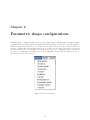
1 Introduction
1.1 Overview of SectionBuilder . . . . . . . . . . . . . . .
1.2 Definition of the beam cross-section . . . . . . . . . .
1.3 Meshing the cross-section . . . . . . . . . . . . . . . .
1.4 Performing the finite element analysis . . . . . . . . .
1.4.1 Sectional properties . . . . . . . . . . . . . . .
1.4.2 Three-dimensional stresses and strains . . . . .
1.5 Visualizing the results . . . . . . . . . . . . . . . . . .
1.5.1 Step 1: Selecting a sectional loading case . . .
1.5.2 Step 2: Selecting the quantities to be visualized
1.5.3 Step 3: Interactive definition of sensors . . . .
1.5.4 The Graphics menu and toolbar . . . . . . . .
1.6 Installation of SectionBuilder . . . . . . . . . . . . . .
1.6.1 Directory structure . . . . . . . . . . . . . . . .
1.6.2 Input files . . . . . . . . . . . . . . . . . . . . .
1.6.3 Output files . . . . . . . . . . . . . . . . . . . .
1.6.4 Installation Procedure . . . . . . . . . . . . . .
.
.
.
.
.
.
.
.
.
.
.
.
.
.
.
.
.
.
.
.
.
.
.
.
.
.
.
.
.
.
.
.
.
.
.
.
.
.
.
.
.
.
.
.
.
.
.
.
.
.
.
.
.
.
.
.
.
.
.
.
.
.
.
.
.
.
.
.
.
.
.
.
.
.
.
.
.
.
.
.
.
.
.
.
.
.
.
.
.
.
.
.
.
.
.
.
.
.
.
.
.
.
.
.
.
.
.
.
.
.
.
.
.
.
.
.
.
.
.
.
.
.
.
.
.
.
.
.
.
.
.
.
.
.
.
.
.
.
.
.
.
.
.
.
.
.
.
.
.
.
.
.
.
.
.
.
.
.
.
.
.
.
.
.
.
.
.
.
.
.
.
.
.
.
.
.
.
.
.
.
.
.
.
.
.
.
.
.
.
.
.
.
.
.
.
.
.
.
.
.
.
.
.
.
.
.
.
.
.
.
.
.
.
.
.
.
.
.
.
.
.
.
.
.
.
.
.
.
.
.
.
.
.
.
.
.
.
.
.
.
.
.
.
.
.
.
.
.
.
.
.
.
.
.
.
.
.
.
.
.
.
.
.
.
.
.
.
.
.
.
.
.
.
.
.
.
.
.
.
.
.
.
.
.
.
.
.
.
.
.
.
.
.
.
.
.
.
.
.
.
.
.
.
.
.
.
.
.
.
.
.
.
.
.
.
.
.
.
.
.
.
.
.
.
.
.
.
.
.
.
.
.
.
.
.
.
.
.
.
.
.
.
.
.
.
.
.
.
.
.
.
.
7
7
8
8
8
9
17
19
19
20
21
23
24
24
25
25
25
2 Parametric shape configurations
2.1 Definition of airfoil sections . . . . .
2.1.1 The Airfoil-section dialog tab
2.1.2 The Airfoil profile dialog tab
2.1.3 The Dimensions dialog tab .
2.1.4 The Materials dialog tab . .
2.1.5 Formatted input . . . . . . .
2.1.6 Examples . . . . . . . . . . .
2.2 Definition of circular arcs . . . . . .
2.2.1 The Circular Arc dialog tab .
2.2.2 The Dimensions dialog tab .
2.2.3 The Materials dialog tab . .
2.2.4 Formatted input . . . . . . .
2.2.5 Examples . . . . . . . . . . .
2.3 Definition of C-sections . . . . . . .
2.3.1 The C-section dialog tab . .
2.3.2 The Dimensions dialog tab .
2.3.3 The Materials dialog tab . .
2.3.4 Formatted input . . . . . . .
2.3.5 Examples . . . . . . . . . . .
2.4 Definition of circular cylinders . . . .
2.4.1 The Cylinder dialog tab . . .
2.4.2 The Dimensions dialog tab .
2.4.3 The Materials dialog tab . .
.
.
.
.
.
.
.
.
.
.
.
.
.
.
.
.
.
.
.
.
.
.
.
.
.
.
.
.
.
.
.
.
.
.
.
.
.
.
.
.
.
.
.
.
.
.
.
.
.
.
.
.
.
.
.
.
.
.
.
.
.
.
.
.
.
.
.
.
.
.
.
.
.
.
.
.
.
.
.
.
.
.
.
.
.
.
.
.
.
.
.
.
.
.
.
.
.
.
.
.
.
.
.
.
.
.
.
.
.
.
.
.
.
.
.
.
.
.
.
.
.
.
.
.
.
.
.
.
.
.
.
.
.
.
.
.
.
.
.
.
.
.
.
.
.
.
.
.
.
.
.
.
.
.
.
.
.
.
.
.
.
.
.
.
.
.
.
.
.
.
.
.
.
.
.
.
.
.
.
.
.
.
.
.
.
.
.
.
.
.
.
.
.
.
.
.
.
.
.
.
.
.
.
.
.
.
.
.
.
.
.
.
.
.
.
.
.
.
.
.
.
.
.
.
.
.
.
.
.
.
.
.
.
.
.
.
.
.
.
.
.
.
.
.
.
.
.
.
.
.
.
.
.
.
.
.
.
.
.
.
.
.
.
.
.
.
.
.
.
.
.
.
.
.
.
.
.
.
.
.
.
.
.
.
.
.
.
.
.
.
.
.
.
.
.
.
.
.
.
.
.
.
.
.
.
.
.
.
.
.
.
.
.
.
.
.
.
.
.
.
.
.
.
.
.
.
.
.
.
.
.
.
.
.
.
.
.
.
.
.
.
.
.
.
.
.
.
.
.
.
.
.
.
.
.
.
.
.
.
.
.
.
.
.
.
.
.
.
.
.
.
.
.
.
.
.
.
.
.
.
.
.
.
.
.
.
.
.
.
.
.
.
.
.
.
.
.
.
.
.
.
.
.
.
.
.
.
.
.
.
.
.
.
.
.
.
.
.
.
.
.
.
.
.
.
.
.
.
.
.
.
.
.
.
.
.
.
.
.
.
.
.
.
.
.
.
.
.
.
.
.
.
.
.
.
.
.
.
.
.
.
.
.
.
.
.
.
.
.
.
.
.
.
.
.
.
.
.
.
.
.
.
.
.
.
.
.
.
.
.
.
.
.
.
.
.
.
.
.
.
.
.
.
.
.
.
27
28
30
31
32
34
35
36
38
39
40
41
42
43
45
46
47
48
56
57
60
61
62
63
.
.
.
.
.
.
.
.
.
.
.
.
.
.
.
.
.
.
.
.
.
.
.
.
.
.
.
.
.
.
.
.
.
.
.
.
.
.
.
.
.
.
.
.
.
.
.
.
.
.
.
.
.
.
.
.
.
.
.
.
.
.
.
.
.
.
.
.
.
.
.
.
.
.
.
.
.
.
.
.
.
.
.
.
.
.
.
.
.
.
.
.
.
.
.
.
.
.
.
.
.
.
.
.
.
.
.
.
.
.
.
.
.
.
.
3
.
.
.
.
.
.
.
.
.
.
.
.
.
.
.
.
.
.
.
.
.
.
.
.
.
.
.
.
.
.
.
.
.
.
.
.
.
.
.
.
.
.
.
.
.
.
.
.
.
.
.
.
.
.
.
.
.
.
.
.
.
.
.
.
.
.
.
.
.
.
.
.
.
.
.
.
.
.
.
.
.
.
.
.
.
.
.
.
.
.
.
.
.
.
.
.
.
.
.
.
.
.
.
.
.
.
.
.
.
.
.
.
.
.
.
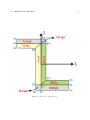
4
CONTENTS
2.4.4 Formatted input . . . . . . . . . . . . .
2.4.5 Examples . . . . . . . . . . . . . . . . .
2.5 Definition of double boxes . . . . . . . . . . . .
2.5.1 The Double Box dialog tab . . . . . . .
2.5.2 The Dimensions dialog tab . . . . . . .
2.5.3 The Materials dialog tab . . . . . . . .
2.5.4 Formatted input . . . . . . . . . . . . .
2.5.5 Examples . . . . . . . . . . . . . . . . .
2.6 Definition of I-sections . . . . . . . . . . . . . .
2.6.1 The I-section dialog tab . . . . . . . . .
2.6.2 The Dimensions dialog tab . . . . . . .
2.6.3 The Materials dialog tab . . . . . . . .
2.6.4 Formatted input . . . . . . . . . . . . .
2.6.5 Examples . . . . . . . . . . . . . . . . .
2.7 Definition of rectangular boxes . . . . . . . . .
2.7.1 The Rectangular box dialog tab . . . . .
2.7.2 The Dimensions dialog tab . . . . . . .
2.7.3 The Materials dialog tab . . . . . . . .
2.7.4 Formatted input . . . . . . . . . . . . .
2.7.5 Examples . . . . . . . . . . . . . . . . .
2.8 Definition of rectangular sections . . . . . . . .
2.8.1 The Rectangular section dialog tab . . .
2.8.2 The Dimensions dialog tab . . . . . . .
2.8.3 The Materials dialog tab . . . . . . . .
2.8.4 Formatted input . . . . . . . . . . . . .
2.8.5 Examples . . . . . . . . . . . . . . . . .
2.9 Definition of circular tubes . . . . . . . . . . .
2.9.1 The Circular tube dialog tab . . . . . .
2.9.2 The Dimensions dialog tab . . . . . . .
2.9.3 The Materials dialog tab . . . . . . . .
2.9.4 Formatted input . . . . . . . . . . . . .
2.9.5 Examples . . . . . . . . . . . . . . . . .
2.10 Definition of triangular sections . . . . . . . . .
2.10.1 The Triangular section name dialog tab
2.10.2 The Dimensions dialog tab . . . . . . .
2.10.3 The Materials dialog tab . . . . . . . .
2.10.4 Formatted input . . . . . . . . . . . . .
2.10.5 Examples . . . . . . . . . . . . . . . . .
2.11 Definition of T-sections . . . . . . . . . . . . .
2.11.1 The T-section dialog tab . . . . . . . .
2.11.2 The Dimensions dialog tab . . . . . . .
2.11.3 The Materials dialog tab . . . . . . . .
2.11.4 Formatted input . . . . . . . . . . . . .
2.11.5 Examples . . . . . . . . . . . . . . . . .
3 Builder
3.1 Introduction . . . . . . . . . .
3.1.1 Examples . . . . . . .
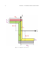
3.2 Definition of walls . . . . . .
3.2.1 Wall geometry . . . .
3.2.2 Wall stacking sequence
3.2.3 Formatted input . . .
3.2.4 Examples . . . . . . .
3.3 Definition of Split sections . .
.
.
.
.
.
.
.
.
.
.
.
.
.
.
.
.
.
.
.
.
.
.
.
.
.
.
.
.
.
.
.
.
.
.
.
.
.
.
.
.
.
.
.
.
.
.
.
.
.
.
.
.
.
.
.
.
.
.
.
.
.
.
.
.
.
.
.
.
.
.
.
.
.
.
.
.
.
.
.
.
.
.
.
.
.
.
.
.
.
.
.
.
.
.
.
.
.
.
.
.
.
.
.
.
.
.
.
.
.
.
.
.
.
.
.
.
.
.
.
.
.
.
.
.
.
.
.
.
.
.
.
.
.
.
.
.
.
.
.
.
.
.
.
.
.
.
.
.
.
.
.
.
.
.
.
.
.
.
.
.
.
.
.
.
.
.
.
.
.
.
.
.
.
.
.
.
.
.
.
.
.
.
.
.
.
.
.
.
.
.
.
.
.
.
.
.
.
.
.
.
.
.
.
.
.
.
.
.
.
.
.
.
.
.
.
.
.
.
.
.
.
.
.
.
.
.
.
.
.
.
.
.
.
.
.
.
.
.
.
.
.
.
.
.
.
.
.
.
.
.
.
.
.
.
.
.
.
.
.
.
.
.
.
.
.
.
.
.
.
.
.
.
.
.
.
.
.
.
.
.
.
.
.
.
.
.
.
.
.
.
.
.
.
.
.
.
.
.
.
.
.
.
.
.
.
.
.
.
.
.
.
.
.
.
.
.
.
.
.
.
.
.
.
.
.
.
.
.
.
.
.
.
.
.
.
.
.
.
.
.
.
.
.
.
.
.
.
.
.
.
.
.
.
.
.
.
.
.
.
.
.
.
.
.
.
.
.
.
.
.
.
.
.
.
.
.
.
.
.
.
.
.
.
.
.
.
.
.
.
.
.
.
.
.
.
.
.
.
.
.
.
.
.
.
.
.
.
.
.
.
.
.
.
.
.
.
.
.
.
.
.
.
.
.
.
.
.
.
.
.
.
.
.
.
.
.
.
.
.
.
.
.
.
.
.
.
.
.
.
.
.
.
.
.
.
.
.
.
.
.
.
.
.
.
.
.
.
.
.
.
.
.
.
.
.
.
.
.
.
.
.
.
.
.
.
.
.
.
.
.
.
.
.
.
.
.
.
.
.
.
.
.
.
.
.
.
.
.
.
.
.
.
.
.
.
.
.
.
.
.
.
.
.
.
.
.
.
.
.
.
.
.
.
.
.
.
.
.
.
.
.
.
.
.
.
.
.
.
.
.
.
.
.
.
.
.
.
.
.
.
.
.
.
.
.
.
.
.
.
.
.
.
.
.
.
.
.
.
.
.
.
.
.
.
.
.
.
.
.
.
.
.
.
.
.
.
.
.
.
.
.
.
.
.
.
.
.
.
.
.
.
.
.
.
.
.
.
.
.
.
.
.
.
.
.
.
.
.
.
.
.
.
.
.
.
.
.
.
.
.
.
.
.
.
.
.
.
.
.
.
.
.
.
.
.
.
.
.
.
.
.
.
.
.
.
.
.
.
.
.
.
.
.
.
.
.
.
.
.
.
.
.
.
.
.
.
.
.
.
.
.
.
.
.
.
.
.
.
.
.
.
.
.
.
.
.
.
.
.
.
.
.
.
.
.
.
.
.
.
.
.
.
.
.
.
.
.
.
.
.
.
.
.
.
.
.
.
.
.
.
.
.
.
.
.
.
.
.
.
.
.
.
.
.
.
.
.
.
.
.
.
.
.
.
.
.
.
.
.
.
.
.
.
.
.
.
.
.
.
.
.
.
.
.
.
.
.
.
.
.
.
.
.
.
.
.
.
.
.
.
.
.
.
.
.
.
.
.
.
.
.
.
.
.
.
.
.
.
.
.
.
.
.
.
.
.
.
.
.
.
.
.
.
.
.
.
.
.
.
.
.
.
.
.
.
.
.
.
.
.
.
.
.
.
.
.
.
.
.
.
.
.
.
.
.
.
.
.
.
.
.
.
.
.
.
.
.
.
.
.
.
.
.
.
.
.
.
.
.
.
.
.
.
.
.
.
.
.
.
.
.
.
.
.
.
.
.
.
.
.
.
.
.
.
.
.
.
.
.
.
.
.
.
.
.
.
.
.
.
.
.
.
.
.
.
.
.
.
.
.
.
.
.
.
.
.
.
.
.
.
.
.
.
.
.
.
.
.
.
.
.
.
.
.
.
.
.
.
.
.
.
.
.
.
.
.
.
.
.
.
.
.
.
.
.
.
.
.
.
.
.
.
.
.
.
.
.
.
.
.
.
.
.
.
.
.
.
.
.
.
.
.
.
.
.
.
.
.
.
.
.
.
.
.
.
.
.
.
.
.
.
.
.
.
.
.
.
.
.
.
.
.
.
.
.
.
.
.
.
.
.
.
.
.
.
.
.
.
.
.
.
.
.
.
.
.
.
.
.
.
.
.
.
.
.
.
.
.
.
.
.
.
.
.
.
.
.
.
.
.
.
.
.
.
.
.
.
.
.
.
.
.
.
.
.
.
.
.
.
.
.
.
.
.
.
.
.
.
.
.
.
.
.
.
.
.
.
.
.
.
.
.
.
.
.
.
.
.
.
.
.
.
.
.
.
.
.
.
.
.
.
.
.
.
.
.
.
.
.
.
.
.
.
.
.
.
.
.
.
.
.
.
.
.
.
.
.
.
.
.
.
.
.
.
.
.
.
.
.
.
.
.
.
.
.
.
.
.
.
.
.
.
.
.
.
.
.
.
.
.
.
.
.
.
.
.
.
.
.
.
.
.
.
.
64
65
66
67
68
70
72
72
74
75
76
78
84
84
88
89
90
92
94
94
96
97
98
99
101
102
104
105
106
107
108
109
111
112
113
114
116
117
118
119
120
121
123
124
.
.
.
.
.
.
.
.
.
.
.
.
.
.
.
.
.
.
.
.
.
.
.
.
.
.
.
.
.
.
.
.
.
.
.
.
.
.
.
.
.
.
.
.
.
.
.
.
.
.
.
.
.
.
.
.
.
.
.
.
.
.
.
.
.
.
.
.
.
.
.
.
.
.
.
.
.
.
.
.
.
.
.
.
.
.
.
.
.
.
.
.
.
.
.
.
.
.
.
.
.
.
.
.
.
.
.
.
.
.
.
.
.
.
.
.
.
.
.
.
.
.
.
.
.
.
.
.
.
.
.
.
.
.
.
.
.
.
.
.
.
.
.
.
.
.
.
.
.
.
.
.
.
.
.
.
.
.
.
.
.
.
.
.
.
.
.
.
.
.
.
.
.
.
.
.
.
.
.
.
.
.
.
.
.
.
.
.
.
.
.
.
.
.
.
.
.
.
.
.
.
.
.
.
.
.
.
.
127
127
127
129
129
129
131
132
134
CONTENTS
.
.
.
.
.
.
.
.
.
.
.
.
.
.
.
.
.
.
.
.
.
.
.
.
.
.
.
.
.
.
.
.
.
.
.
.
.
.
.
.
.
.
.
.
.
.
.
.
.
.
.
.
.
.
.
.
.
.
.
.
.
.
.
.
.
.
.
.
.
.
.
.
.
.
.
.
.
.
.
.
.
.
.
.
.
.
.
.
.
.
.
.
.
.
.
.
.
.
.
.
.
.
.
.
.
.
.
.
.
.
.
.
.
.
.
.
.
.
.
.
.
.
.
.
.
.
.
.
.
.
.
.
.
.
.
.
.
.
.
.
.
.
.
.
.
.
.
.
.
.
.
.
.
.
.
.
.
.
.
.
.
.
.
.
.
.
.
.
.
.
.
.
.
.
.
.
.
.
.
.
.
.
.
.
.
.
.
.
.
.
.
.
136
137
138
141
142
144
146
147
4 Material properties
4.1 Definition of material properties . . . . . . . . . . .
4.1.1 The Material properties dialog window . . . .
4.1.2 The Stiffness dialog window . . . . . . . . . .
4.1.3 The Failure Criterion dialog window . . . . .
4.1.4 The Strength dialog window . . . . . . . . . .
4.1.5 Formatted input . . . . . . . . . . . . . . . .
4.2 Definition of solid properties . . . . . . . . . . . . . .
4.2.1 The Solid material properties dialog window .
4.2.2 The Layer List dialog window . . . . . . . . .
.
.
.
.
.
.
.
.
.
.
.
.
.
.
.
.
.
.
.
.
.
.
.
.
.
.
.
.
.
.
.
.
.
.
.
.
.
.
.
.
.
.
.
.
.
.
.
.
.
.
.
.
.
.
.
.
.
.
.
.
.
.
.
.
.
.
.
.
.
.
.
.
.
.
.
.
.
.
.
.
.
.
.
.
.
.
.
.
.
.
.
.
.
.
.
.
.
.
.
.
.
.
.
.
.
.
.
.
.
.
.
.
.
.
.
.
.
.
.
.
.
.
.
.
.
.
.
.
.
.
.
.
.
.
.
.
.
.
.
.
.
.
.
.
.
.
.
.
.
.
.
.
.
.
.
.
.
.
.
.
.
.
.
.
.
.
.
.
.
.
.
.
.
.
.
.
.
.
.
.
.
.
.
.
.
.
.
.
.
.
.
.
.
.
.
.
.
.
.
.
.
.
.
.
.
.
.
149
151
152
154
156
158
159
160
161
162
3.4
3.5
3.3.1 Formatted input . .
3.3.2 Examples . . . . . .
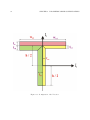
Definition of Tcon sections .
3.4.1 Formatted input . .
3.4.2 Examples . . . . . .
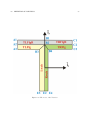
Definition of Vcon sections
3.5.1 Formatted input . .
3.5.2 Examples . . . . . .
5
.
.
.
.
.
.
.
.
.
.
.
.
.
.
.
.
.
.
.
.
.
.
.
.
.
.
.
.
.
.
.
.
.
.
.
.
.
.
.
.
.
.
.
.
.
.
.
.
.
.
.
.
.
.
.
.
.
.
.
.
.
.
.
.
.
.
.
.
.
.
.
.
.
.
.
.
.
.
.
.
.
.
.
.
.
.
.
.
.
.
.
.
.
.
.
.
.
.
.
.
.
.
.
.
5 Mesh density
165
5.1 Example . . . . . . . . . . . . . . . . . . . . . . . . . . . . . . . . . . . . . . . . . . . . . . . . 165
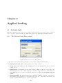
6 Applied loading
167
6.1 Sectional loads . . . . . . . . . . . . . . . . . . . . . . . . . . . . . . . . . . . . . . . . . . . . 167
6.1.1 The Sectional loads dialog window . . . . . . . . . . . . . . . . . . . . . . . . . . . . . 167
7 Geometric elements
171
7.1 Definition of fixed frames . . . . . . . . . . . . . . . . . . . . . . . . . . . . . . . . . . . . . . 171
7.2 The Fixed frame dialog window . . . . . . . . . . . . . . . . . . . . . . . . . . . . . . . . . . . 171
7.2.1 Formatted input . . . . . . . . . . . . . . . . . . . . . . . . . . . . . . . . . . . . . . . 171
8 Utility objects
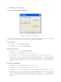
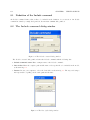
8.1 Definition of the Include command . .
8.2 The Include command dialog window .
8.2.1 Formatted input . . . . . . . .
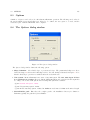
8.3 Options . . . . . . . . . . . . . . . . .
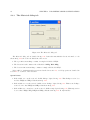
8.4 The Options dialog window . . . . . .
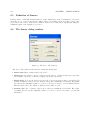
8.5 Definition of Sensors . . . . . . . . . .
8.6 The Sensor dialog window . . . . . . .
.
.
.
.
.
.
.
.
.
.
.
.
.
.
.
.
.
.
.
.
.
.
.
.
.
.
.
.
.
.
.
.
.
.
.
.
.
.
.
.
.
.
.
.
.
.
.
.
.
.
.
.
.
.
.
.
.
.
.
.
.
.
.
.
.
.
.
.
.
.
.
.
.
.
.
.
.
.
.
.
.
.
.
.
.
.
.
.
.
.
.
.
.
.
.
.
.
.
.
.
.
.
.
.
.
.
.
.
.
.
.
.
.
.
.
.
.
.
.
.
.
.
.
.
.
.
.
.
.
.
.
.
.
.
.
.
.
.
.
.
.
.
.
.
.
.
.
.
.
.
.
.
.
.
.
.
.
.
.
.
.
.
.
.
.
.
.
.
.
.
.
.
.
.
.
.
.
.
.
.
.
.
.
.
.
.
.
.
.
.
.
.
.
.
.
.
.
.
.
.
.
.
.
.
.
.
.
.
.
.
.
.
.
.
.
.
.
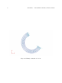
173
174
174
176
177
177
178
178
6
CONTENTS
Chapter 1
Introduction
1.1
Overview of SectionBuilder
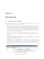
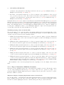
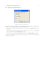
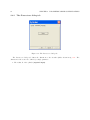
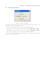
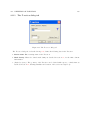
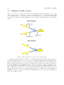
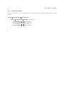
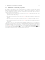
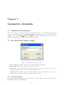
SectionBuilder analyzes beam cross-sections. The analysis proceeds in four steps. The menu of SectionBuilder, depicted in fig. 1.1, reflects these four steps.
1. First, the configuration of the cross-section is defined, this step is discussed in section 1.2. The twodimensional geometric configuration of the section must be defined, together with the physical properties of the materials it is made of. Two avenues are available for this step. First, parametric shapes
can be used, such as I-sections, C-sections, or a variety of commonly used cross-section. Second, more
complex sections of arbitrary configuration can be constructed. The process of defining the section
involves a number a dialog windows described in chapter 2 for the parametric shapes and in chapter 3
for complex sections of arbitrary configuration.
2. Second, a finite element mesh of this two-dimensional problem is created, as discussed in section 1.3.
Clicking the first icon of the menu shown in fig. 1.1 will launch the mesh generation phase of the
analysis.
3. Next, the finite element analysis of the problem is run to compute sectional properties and stress
distributions for given sectional loads. Clicking the second icon of the menu shown in fig. 1.1 will
launch the finite element analysis of the section.
4. The last step of the process is the visualization of all results. Principal axes of bending, shearing and
inertia are displayed together with the centroid, shear center and center of mass. Axial and shear stress
or strain distributions associated with a given sectional loading can also be visualized. Clicking the
third icon of the menu will invoke the visualization program, a detailed discussion of this topic appears
in section 1.5.
Figure 1.1: The SectionBuilder toolbar.
7
8
CHAPTER 1. INTRODUCTION
1.2
Definition of the beam cross-section
The definition of the configuration of the beam’s cross-section involves two main components: the twodimensional geometric configuration of the section, and the physical properties of the materials of which it
is made.
• The geometric configuration of the cross-section can be defined in two alternative manners
1. First, parametric shapes can be used, as discussed in detail in chapter 2. The following parametric
shapes can be defined: airfoil sections as described in section 2.1, circular arcs as described in
section 2.2, C-sections as described in section 2.3, circular cylinders as described in section 2.4,
double boxes as described in section 2.5, I-sections as described in section 2.6, rectangular boxes as
described in section 2.7, rectangular sections as described in section 2.8, circular tubes as described
in section 2.9, triangular sections as described in section 2.10, and T-sections as described in
section 2.11. The various configurations are parametrized, and hence, each section is readily
defined by a small number of input parameters.
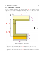
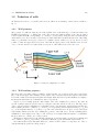
2. Second, more complex sections of arbitrary configuration can be constructed, as discussed in
chapter 3. The definition process is tailored towards the definition of composite structures: layers
of material are stacked in a mold of arbitrary shape; ply insertions or drop-offs are allowed. The
resulting unit is called a “wall.” It is then possible to connect several walls to create complex
sections of arbitrary configuration. The definition of walls is detailed in section 3.2; the following
connectors are available: split-connectors as described in section 3.3, T-connectors as described
in section 3.4 and V-connectors as described in section 3.5.
• The physical properties of the materials the section is made of can be defined in two alternative
manners.
1. Section 4.1 discusses the definition of material properties. Three types of materials can be defined:
isotropic, orthotropic and transversely isotropic materials. Material stiffness, strength and density
can be defined, and a failure criterion can be selected.
2. Section 4.2 discusses the definition of solid properties. In this case, a layered material structure
is defined; each layer features its proper material, ply thickness and fiber orientation angles.
1.3
Meshing the cross-section
Once the configuration of the cross-section has been defined a finite element mesh discretization is created
by clicking the first icon of the SectionBuilder toolbar shown in fig. 1.1. A mapped mesh of the section
is created. The meshing process recognizes the potential presence of layered materials: each layer is meshed
independently to avoid smearing of the material properties. Meshes featuring finite elements of decreasing
sizes can be created by specifying a mesh density parameter.
1.4
Performing the finite element analysis
Next, the mapped mesh generated in the previous step is used as the basis for a finite element analysis of the
section launched by clicking the second icon of the SectionBuilder toolbar shown in fig. 1.1. The finite
element analysis computes the three dimensional warping deformation field over the cross-section. Based
on this warping field, the sectional stiffness and mass matrices are computed as well as three-dimensional
stresses and strains at any location in the section. The predictions of the analysis are summarized in two files;
the first details the sectional properties as described in section 1.4.1, and the second provides the the three
dimensional stresses and strains at user specified location of the cross section as described in section 1.4.2.
1.4. PERFORMING THE FINITE ELEMENT ANALYSIS
1.4.1
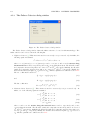
9
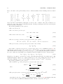
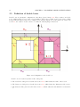
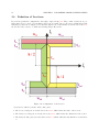
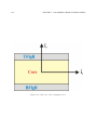
Sectional properties
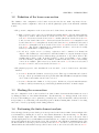
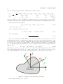
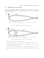
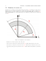
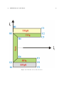
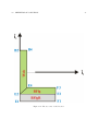
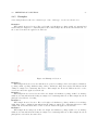
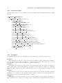
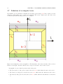
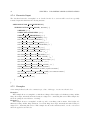
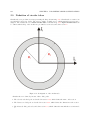
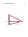
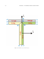
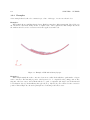
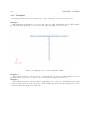
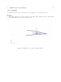
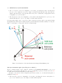
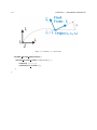
The geometry of the cross-section is described in an orthonormal basis I = (ı̄1 , ı̄2 , ı̄3 ), where ı̄1 , ı̄2 and ı̄3 are
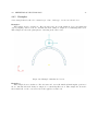
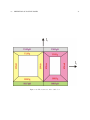
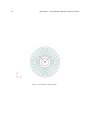
three mutually orthogonal, unit vectors. The plane of the cross section is assumed to coincide with plane
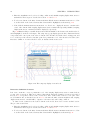
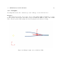
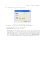
(ı̄2 , ı̄3 ), and the axis of the beam is along unit vector ı̄1 , as depicted in fig. 1.2. The reference axis of the
beam is a line along axis ı̄1 ; the origin of the coordinate system is at the intersection of the reference axis
with the plane of the cross-section. This axis origin is not necessarily at the centroid and can be anywhere
that is convenient. A detailed description of the sectional properties is printed in an output file of extension
.sbp as described in section 1.6.3. This file contains the information detailed in the sections below.
Figure 1.2: Sign conventions for the externally applied force and moment components acting on the crosssection.
Sectional stiffness and compliance matrices
The following sectional stiffness and compliance matrices are computed.
• The 4×4 sectional stiffness matrix. This matrix relates the sectional axial strain, ε1 , twisting curvature,
κ1 , and two bending curvatures, κ2 and κ3 , to the axial force, N1 , twisting moment, M1 , and two
bending moments, M2 and M3 . The relationship between these sectional strains and sectional stress
resultants takes the form of a 4 × 4 matrix,


N1 C11 C14 C15 C16 ε1 M1  C41 C44 C45 C46  κ1 

(1.1)
M2 =  C51 C54 C55 C56  κ2 .
M3 C61 C64 C65 C66 κ3 • The 6 × 6 sectional stiffness matrix, C. This matrix relates the sectional axial strain, ε1 , transverse
shearing strains, ε2 and ε3 , twisting curvatures, κ1 and two bending curvatures, κ2 and κ3 , to the axial
force, N1 , transverse shear forces, V2 and V3 , twisting moment, M1 , and two bending moments, M2
and M3 . The relationship between these sectional strains and sectional stress resultants takes the form
of a symmetric, 6 × 6 matrix


N1 C11 C12 C13 C14 C15 C16 ε1 V2  C12 C22 C23 C24 C25 C26  ε2 

V3  C13 C23 C33 C34 C35 C36  ε3 =

(1.2)
M1  C14 C24 C34 C44 C45 C46  κ1 , or F = C .


M2  C15 C25 C35 C45 C55 C56  κ2 M3 C16 C26 C36 C46 C56 C66 κ3 10
CHAPTER 1. INTRODUCTION
The three forces N1 , V2 and V3 are positive along axes ı̄1 , ı̄2 and ı̄3 , respectively, whereas moments
M1 , M2 and M3 are positive about axes ı̄1 , ı̄2 and ı̄3 , respectively, as depicted in fig. 1.2. Identical sign
conventions are used for the three strains, ε1 , ε2 and ε3 , and curvatures κ1 , κ2 and κ3 , respectively.
The three forces are the resultants of the stress distributions over the cross section; the three moments
are computed with respect to the origin of the coordinate system, i.e. with respect to the reference
axis of the beam, as depicted in fig. 1.2.
• The 6 × 6 sectional compliance matrix, S, the inverse of the sectional stiffness matrix, i.e. S = C −1 ,
and hence,
(1.3)
= S F.
It is often the case that the 6 × 6 stiffness matrix
terms and presents the following structure

N1 C11
0
0
V2  0
C
C
22
23

V3  0
C
C
23
33

M1 =  0
C
C
24
34

M2  C15
0
0
M3 C16
0
0
In such cases, the complete problem
following 3 × 3 stiffness matrix
defined by eq. (1.2) contains a number of vanishing
0
C24
C34
C44
0
0
C15
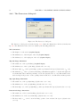
0
0
0
C55
C56
C16
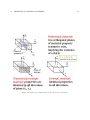
0
0
0
C56
C66








ε1
ε2
ε3
κ1
κ2
κ3
.
splits into an axial force-bending moment problem characterized by the
N1
M2
M3

C11
=  C15
C16
C15
C55
C56

C16 ε1
C56  κ2
C66 κ3
,
and a twisting moment-shear force problem characterized

M1 C44 C24
V2 =  C24 C22
V3 C34 C23
by the following 3 × 3 stiffness matrix

C34 κ1 C23  ε2 .
C33 ε3 The corresponding compliance matrices
ε1
κ2
κ3
and
(1.4)
(1.5)
(1.6)
are

S11
=  S15
S16
S15
S55
S56

S16 N1
S56  M2
S66 M3
,
(1.7)

κ1 S44
ε2 =  S24
ε3 S34
S24
S22
S23

S34 M1
S23  V2
S33 V3
.
(1.8)
for the axial force-bending moment and twisting moment-shear force problems, respectively.
The axial force-bending moment problem
If the stiffness matrix of the cross-section presents the special structure displayed in eq. (1.4), it becomes
possible to separately analyze the axial force-bending moment and twisting moment-shear force problems.
The former problem is the focus of this section.
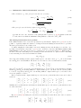
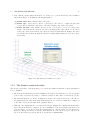
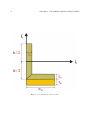
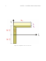
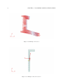
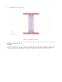
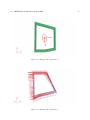
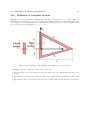
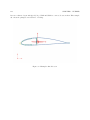
To further simplify the relationship between the axial forces and bending moment and the corresponding
sectional strain components, eq. (1.5), it is convenient to introduce the centroid of the cross-section, a
point of the cross-section with coordinates (xc2 , xc3 ), as depicted in fig. 1.3. With the help of the centroid, the
relationship between axial force and axial strain decouples from the relationship between bending moments
and curvatures,
N1c = S εc1 .
(1.9)
1.4. PERFORMING THE FINITE ELEMENT ANALYSIS
11
where N1c = N1 is the axial force, εc1 the axial strain at the centroid and S the axial stiffness. The bending
moments are related to the sectional curvatures,
c c
c
κ2 M2c H22
−H23
c (1.10)
c
c
κ3 M3c = −H23
H33
where M2c and M3c are the bending moments computed with respect to the centroid about axes parallel to
c
c
ı̄2 and ı̄3 , respectively, κc2 = κ2 and κc3 = κ3 the sectional curvatures, H22
and H33
the bending stiffnesses
c
computed with respect to the centroid about axes parallel to ı̄2 and ı̄3 , respectively, and H23
the cross
bending stiffness computed with respect to the centroid about axes parallel to ı̄2 and ı̄3 .
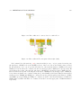
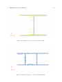
Figure 1.3: Left figure: forces and moments applied at the reference point. Right figure: forces and moments
applied at the centroid.
The forces and moments computed with
as follows


N1 1
0 0 M2 =  xc3 1 0  M3 −xc2 0 1 respect to the reference point
c 
N1 N1c 1
M2c =  −xc3
M2c ;
M3c M3c xc2
and the centroid can be related

0 0 N1 1 0  M2 .
(1.11)
0 1 M3 Similarly, the sectional strains and curvatures with respect to the reference point and the centroid can be
related as follows

c 


ε1 ε1 1 xc3 −xc2 εc1 1 −xc3 xc2 ε1 κ2 =  0 1
κc2 =  0
0  κc2 ;
1
0  κ2 .
(1.12)
c c κ3 κ3 0 0
1
κ3
κ3
0
0
1
Eqs. (1.9) and (1.10) relating the sectional
matrix equation as
c 
N1 M2c = 
M3c forces and strains about the centroid can be recast in a single
S
0
0
0
c
H22
c
−H23
 c
ε1
0
c 
−H23 κc2
c
κc3
H33
.
(1.13)
Introducing eqs. (1.11) and (1.12), the relationship between the corresponding quantities at the reference
point are readily found as


N1 ε1 S
xc3 S
−xc2 S
c
c
M2 =  xc3 S
H22
+ x2c3 S
−(H23
+ xc2 xc3 S)  κ2 .
(1.14)
c
c
M3 κ3 −xc2 S −(H23
+ xc2 xc3 S)
H33
+ x2c2 S
12
CHAPTER 1. INTRODUCTION
The corresponding bending compliance matrix is then found by inversion

∆H
c
c
c
c
c
ε1 + x2c2 H22
+ x2c3 H33
− 2xc2 xc3 H23
xc2 H23
− xc3 H33
1

S
κ2 =
c
c
c

xc2 H23
− xc3 H33
H33
κ3 ∆ H
c
c
c
xc2 H22 − xc3 H23
H23
c
c
xc2 H22
− xc3 H23
c
H23
c
H22

N1
  M2
M3
,
(1.15)
c
c
c 2
where ∆H = H22
H33
− (H23
) . Identifying the compliance matrices in eqs. (1.7) and (1.15), it is possible to
compute from the terms of the compliance matrix the various engineering sectional stiffnesses listed below.
• The centroidal bending stiffnesses,
c
H22
= S66 /∆S ,
c
H33
= S55 /∆S ,
c
H23
= S56 /∆S ,
(1.16)
c
c
x3c = H23
S16 − H22
S15 .
(1.17)
2
where ∆S = S55 S66 − S56
.
• The coordinates of the centroid location,
c
c
x2c = H33
S16 − H23
S15 ,
• The axial stiffness,
S=
1
.
S11 − x2c S16 + x3c S15
(1.18)
Eq. (1.10) describes the bending behavior of the cross-section, but due to the presence of the cross
c
bending stiffness term, H23
, bending in the two planes (ı̄1 , ı̄2 ) and (ı̄1 , ı̄3 ) is coupled. It is possible to define
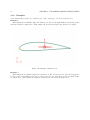
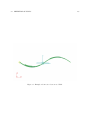
the principal centroidal axes of bending. As illustrated in fig. 1.4, the principal centroidal axes of bending,
b∗ b∗
∗
I b∗ = (ı̄b∗
1 , ı̄2 , ı̄3 ), correspond to a planar rotation of orthonormal basis I by an angle αb ; note that clearly,
b∗
ı̄1 = ı̄1 . When using the principal centroidal axes of bending, the axial forces and bending moments are
fully uncoupled,
c∗ c∗
c∗ c∗
N1c∗ = S εc∗
M2c∗ = H22
κ2 ; M3c∗ = H33
κ3 .
(1.19)
1 ,
c
Clearly, N1c∗ = N1c and εc∗
1 = ε1 , since the rotation of the axis system takes place about unit vector ı̄1 .
c∗
b∗
The bending moments M2 and M3c∗ are computed with respect to the centroid along axes ı̄b∗
2 and ı̄3 ,
c∗
c∗
b∗
b∗
respectively. Similarly, κ2 and κ3 are the sectional curvatures about axes ı̄2 and ı̄3 , respectively.
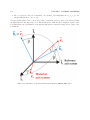
Figure 1.4: Orientation of the principal axes of bending.
The following quantities are also provided.
1.4. PERFORMING THE FINITE ELEMENT ANALYSIS
13
• The orientation, αb∗ , of the principal centroidal axes of bending,
sin 2αb∗ =
where
c
H23
,
∆
s
∆=
cos 2αb∗ =
c − Hc
H33
22
2
2
c
c
H33
− H22
,
2∆
(1.20)
c )2 .
+ (H23
(1.21)
c∗
c∗
• The principal centroidal bending stiffnesses, H22
and H33
,
c∗
H22
=
c
c
H33
+ H22
− ∆,
2
c∗
H33
=
c
c
H33
+ H22
+ ∆.
2
(1.22)
Note that the choice the orientation of the principal axis ı̄b∗
2 given by eq. (1.20) guarantees that axis
c∗
c∗
ı̄b∗
2 is the axis about which the minimum bending stiffness occurs; hence, H22 ≤ H33 .
The twisting moment-shear force problem
If the stiffness matrix of the cross-section presents the special structure displayed in eq. (1.4), it becomes
possible to separately analyze the axial force-bending moment and twisting moment shear force problems.
The latter problem is the focus of this section.
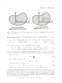
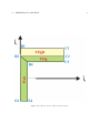
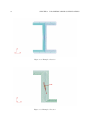
To further simplify the relationship between the twisting moment and shearing forces and the corresponding sectional strain components, eq. (1.6), it is convenient to introduce the shear center of the
cross-section, a point of the cross-section of coordinates (xk2 , xk3 ), as depicted in fig. 1.5. With the help of
the shear center, the relationship between twisting moment and twist rate decouples from the relationship
between shearing forces and sectional transverse strains,
k
M1k = H11
κk1 ;
(1.23)
where M1k is the twisting moment computed with respect to the shear center, εk1 = ε1 the sectional twist
k
rate and H11
the torsional stiffness. The shear forces are related to the sectional transverse strains,
k k k
k
V2 γ12 K22
−K23
k =
k (1.24)
k
k
V3 γ13 −K23
K33
k
k
where V2k = V2 and V3k = V3 are the sectional shearing forces, γ12
and γ13
the sectional transverse shearing
k
k
strains, K22 and K33 the shearing stiffnesses computed with respect to the shear center about axes parallel
k
to ı̄2 and ı̄3 , respectively, and K23
the cross shearing stiffness computed with respect to the shear center
about axes parallel to ı̄2 and ı̄3 .
The forces and moments computed with respect to the reference point and the shear center can be related
as follows




M1 M1k 1 −xk3 xk2 M1k 1 xk3 −xk2 M1 V2 =  0
V2k =  0 1
1
0  V2k ;
0  V2 .
(1.25)
k k
V3 V3 0
0
1
0 0
1
V3
V3
Similarly, the sectional twist rate and
are related as follows

κ1 1
0
γ12 =  xk3 1
γ13 −xk2 0
transverse strains with respect to the reference point and shear center
Eqs. (1.23) and (1.24) relating the
matrix form as
M1k
k
V2
k
V
3
sectional forces and strains about the shear center can be recast in a
 k
 k κ1 H11
0
0
k k
k 
= 0
.
K
−K
(1.27)
22
23
γ12
k
k
γk 0
−K23
K33
13

0 κk1
k
0  γ12
k
1
γ13
;
k
κ1
k
γ12
k
γ
13

1
=  −xk3
xk2

0 0 κ1
1 0  γ12
0 1 γ13
.
(1.26)
14
CHAPTER 1. INTRODUCTION
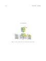
Figure 1.5: Left figure: forces and moments applied at the reference point. Right figure: forces and moments
applied at the shear center.
Introducing eqs. (1.25) and (1.26), the relationship between the corresponding quantities at the reference
point are readily found as


k
k
k
k
k
k
k
M1 κ1 H11 + x2k2 K33
+ x2k3 K22
+ 2xk2 xk3 K23
−xk2 K23
− xk3 K22
xk2 K33
+ xk3 K23
k
k
k
k
V2 = 
 γ12 −xk2 K23
− xk3 K22
K22
−K23
k
k
k
k
V3 γ13 xk2 K33
+ xk3 K23
−K23
K33
(1.28)
The corresponding bending compliance matrix is then found by inversion


κ1 M1 1/H11
xk3 /H11
−xk2 /H11
k
k
γ12 =  xk3 /H11
K33
/∆K + x2k3 /H11
K23
/∆K − xk2 xk3 /H11  V2 ,
(1.29)
k
k
γ13 V3 −xk2 /H11 K23
/∆K − xk2 xk3 /H11
K22
/∆K + x2 /H11
k2
k
k
k 2
where ∆K = K22
K33
− (K23
) . Identifying the compliance matrices in eqs. (1.8) and (1.29), it is possible to
compute from the terms of the compliance matrix the various engineering sectional stiffnesses listed below.
• The torsional stiffness,
H11 =
1
.
S44
(1.30)
• The coordinates of the shear center,
x2k = −H11 S34 ,
x3k = H11 S24 .
(1.31)
• The shearing stiffnesses about shear center,
k
K22
= b∆K ,
k
K33
= a∆K ,
k
K23
= c∆K ,
(1.32)
where a = S22 − x23k /H11 , b = S33 − x22k /H11 , c = S23 + x2k x3k /H11 and ∆ = 1/(ab − c2 ).
Eq. (1.24) describes the shearing behavior of the cross-section, but due to the presence of the cross
k
shearing stiffness term, K23
, shearing in the two planes (ı̄1 , ı̄2 ) and (ı̄1 , ı̄3 ) is coupled. It is possible to define
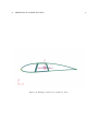
the principal axes of shearing at the shear center. As illustrated in fig. 1.6, the principal axes of shearing
s∗ s∗
at the shear center, I ∗ = (ı̄s∗
1 , ı̄2 , ı̄3 ), correspond to a planar rotation of orthonormal basis I by an angle
∗
s∗
αs ; note that clearly, ı̄1 = ı̄1 . When using the principal axes of shearing at the shear center, the twisting
moment and shearing forces are fully uncoupled,
k
M1k∗ = H11
κk∗
1 ,
k∗ k∗
V2k∗ = K22
γ12 ;
k∗ k∗
V3k∗ = K33
γ13 .
(1.33)
1.4. PERFORMING THE FINITE ELEMENT ANALYSIS
15
k
Clearly, M1k∗ = M1k and κk∗
1 = κ1 , since the rotation of the axis system takes place about unit vector ı̄1 .
s∗
The shearing forces V2k∗ and V3k∗ are computed with respect to the shear center along axes ı̄s∗
2 and ı̄3 ,
k∗
k∗
s∗
respectively. Similarly, γ12
and γ13
are the sectional transverse strains along axes ı̄s∗
and
ı̄
,
respectively.
2
3
Figure 1.6: Orientation of the principal axes of shearing.
The following quantities are also provided.
• The orientation, αs∗ , of the principal axes of shearing at the shear center,
sin 2αs∗ =
where
k
K23
,
∆
s
∆=
cos 2αs∗ = −
k − Kk
K33
22
2
2
k
k
K33
− K22
,
2∆
k )2 .
+ (K23
(1.34)
(1.35)
k∗
k∗
• The principal shearing stiffnesses at the shear center, K22
and K33
,
k∗
K22
=
k
k
K33
+ K22
− ∆,
2
k∗
K33
=
k
k
K33
+ K22
+ ∆.
2
(1.36)
Note that the choice the orientation of the principal axis ı̄s∗
2 given by eq. (1.34) guarantees that axis
k∗
k∗
ı̄s∗
is
the
axis
along
which
the
minimum
shearing
stiffness
occurs;
hence, K22
≤ K33
.
2
Sectional masses and moments of inertia
The 6 × 6 sectional mass matrix, M . This matrix relates the sectional linear velocities, denoted v1 , v2 and v3 ,
and angular velocities, denoted ω1 , ω2 and ω3 , to the sectional linear momenta, denoted p1 , p2 and p3 , and
angular momenta, denoted h1 , h2 and h3 . The relationship between these sectional velocities and sectional
momenta takes the form of a symmetric, 6 × 6 matrix


p1 M11 M12 M13 M14 M15 M16 v1 p2  M12 M22 M23 M24 M25 M26  v2 

p3  M13 M23 M33 M34 M35 M36  v3 
=
(1.37)
h1  M14 M24 M34 M44 M45 M46  ω1 .


h2  M15 M25 M35 M45 M55 M56  ω2 h3 M16 M26 M36 M46 M56 M66 ω3 16
CHAPTER 1. INTRODUCTION
Due to the
as
p1
p2
p3
h1
h2
h3
nature of the problem, many of these coefficients vanish, and the remaining entries are written

m00

0


0
=

0

 m00 x3m
−m00 x2m
0
m00
0
−m00 x3m
0
0
0
0
m00
m00 x2m
0
0
0
m00 x3m
0
0
0
I22
I23
−m00 x3m
m00 x2m
I11
0
0
−m00 x2m
0
0
0
I23
I33








v1
v2
v3
ω1
ω2
ω3
,
(1.38)
where m00 is the sectional mass per unit span, x2m and x3m the coordinates of the center of mass, I22 , I33
and I23 the components of the sectional mass moments of inertia per unit span, and I11 the sectional polar
moment of inertia per unit span.
The following quantities are also provided.
• The sectional area, A.
• The sectional mass per unit span,
m00 = M11 = M22 = M33 .
(1.39)
• The location of the mass center,
x2m =
M34
,
m00
x3m =
M15
.
m00
(1.40)
• The mass moments of inertia per unit span about the center of mass,
m
I22
= I22 − m00 x2m3 ,
m
I33
= I33 − m00 x2m2 ,
m
I23
= I23 + m00 xm2 xm3 .
(1.41)
• The polar moment of inertia per unit span about the center of mass,
m
m
m
I11
= I22
+ I33
.
(1.42)
It is possible to define the principal axes of inertia at the center of mass. As illustrated in fig. 1.7, the
m∗ m∗
principal axes of inertia at the center of mass, I m∗ = (ı̄m∗
1 , ı̄2 , ı̄3 ), correspond to a planar rotation of
∗
m∗
orthonormal basis I by an angle αm ; about ı̄1 so that, ı̄1 = ı̄1 . When using the principal axes of inertia at
the center of mass, the relationship between angular momenta and angular velocities so that uncouples
m
∗
hm∗
1 = I11 ω1 ,
m∗ ∗
hm∗
2 = I22 ω2 ;
m∗ ∗
hm∗
3 = I33 ω3 .
(1.43)
m
∗
Clearly, hm∗
1 = h1 and ω1 = ω1 , since the rotation of the axis system takes place about unit vector ı̄1 . The
m∗
angular momenta h2 and hm∗
are computed with respect to the center of mass along axes ı̄m∗
and ı̄m∗
3
2
3 ,
∗
∗
m∗
m∗
respectively. Similarly, ω2 and ω3 are the angular velocities about axes ı̄2 and ı̄3 , respectively.
The following quantities are also provided.
∗
• The orientation, αm
, of the principal axes of inertia at the center of mass,
∗
sin 2αm
=−
where
m
I23
,
∆
s
∆=
∗
cos 2αm
=
m − Im
I33
22
2
2
m
m
− I22
I33
,
2∆
m )2 .
+ (I23
(1.44)
(1.45)
m∗
m∗
• The principal moments of inertia per unit span about center of mass, I22
and I33
,
m∗
I22
=
m
m
I33
+ I22
− ∆,
2
m∗
I33
=
m
m
I33
+ I22
+ ∆.
2
(1.46)
Note that the choice the orientation of the principal axis ı̄m∗
given by eq. (1.44) guarantees that axis
2
m∗
m∗
ı̄m∗
is
the
axis
about
which
the
minimum
moments
of
inertia
occurs;
hence, I22
≤ I33
.
2
1.4. PERFORMING THE FINITE ELEMENT ANALYSIS
17
Figure 1.7: Orientation of the principal axes of inertia at the center of mass.
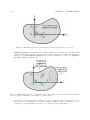
1.4.2
Three-dimensional stresses and strains
The geometry of the cross-section is described in an orthonormal basis I = (ı̄1 , ı̄2 , ı̄3 ), where ı̄1 , ı̄2 and ı̄3 are
three mutually orthogonal, unit vectors. The plane of the cross section is assumed to coincide with plane
(ı̄2 , ı̄3 ), and the axis of the beam is along unit vector ı̄1 , as depicted in fig. 1.2. The reference axis of the
beam is a line along axis ı̄1 ; the origin of the coordinate system is at the intersection of the reference axis
with the plane of the cross-section.
To compute three-dimensional warping displacement, stress components or strain components, two user
defined inputs are required.
1. First, sectional loading cases must be defined as described in section 6.1. A loading case consists of an
axial force and two transverse shear forces, as well as a twisting moment and two bending moments,
applied to the cross-section. These 3 forces and 3 moments can be applied at the reference axis, at the
centroid, at the shear center, or at an arbitrary point of the cross-section.
2. Second, sensors must be defined as described in section 8.5. These “sensors” are analogous to their
physical counterparts, such as strain gauges, which provide information about the local strain field.
Sensors define the location on the cross-section where the information will be computed and the type
of quantity to be sensed, which could be three-dimensional warping displacement, stress components
or strain components.
For each of the defined loading cases, the quantities measured by each of the sensors will be computed and
printed. A detailed report is printed in an output file with extension .sbs as described in section 1.6.3.
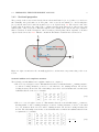
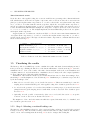
Warping displacements
Under the effect of the applied loading, the cross-section will deform. This deformation is characterized
by a three-dimensional warping displacement field, which features components both in- and out-of-plane
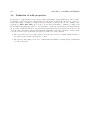
of the cross-section. A typical print-out of a warping sensor is shown in Table 1.1. For the sensor named
SensorWarping, the out-of-plane warping displacement component, w1 , as well as the in-plane warping
displacement components, w2 and w3 , are listed at the sensor location. The displacement components w1 ,
w2 and w3 are the components of the displacement vector along unit vectors ı̄1 , ı̄2 and ı̄3 , respectively.
18
CHAPTER 1. INTRODUCTION
— Sensor : [SensorWarping].
Sensor location (x2 , x3 )
Section warping: w1 , w2 , w3
=
=
(-1.9e-18, -7.4e-02) [m].
( 0.0e+00, -3.9e-09, 4.8e-09) [m].
Table 1.1: Print-out of the three-dimensional warping displacement at a sensor location.
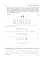
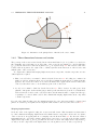
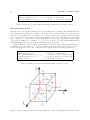
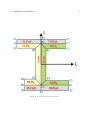
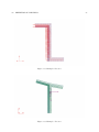
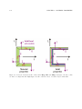
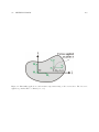
Three-dimensional stresses
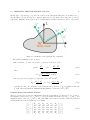
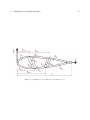
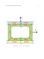
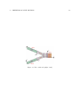
Under the effect of the applied loading, the cross-section will deform, generating a three-dimensional stress
field, which features both in- and out-of-plane components on the cross-section. Since the cross-section is in
plane (ı̄2 , ı̄3 ), the in-plane stress components are σ2 , τ23 and σ3 , whereas the out-of-plane stress components
are σ1 , τ12 and τ13 as described in fig. 1.8. Note that classical beam theory predicts only the the out-of-plane
stress component, σ1 , and the two transverse shearing stresses, τ12 and τ13 ; typically, the in-plane stress
components are assumed to be negligible, i.e. σ2 ≈ 0, τ23 ≈ 0 and σ3 ≈ 0. The analysis implemented in
SectionBuilder predicts both out-of-plane and in-plane stress components.
A typical print-out of a stress sensor is shown in Table 1.2. For the sensor named SensorStresses, the
out-of-plane stress components, σ1 , τ12 and τ13 , as well as the in-plane stress components, σ2 , τ23 and σ3 ,
are listed at the sensor location. Fig. 1.8 shows the sign convention used for the stress computation.
--- Sensor : [SensorStresses].
Sensor location (x2 , x3 )
Out-of-plane stresses: σ1 , τ12 , τ13
In-plane stresses: σ2 , τ23 , σ3
Reserve factors
=
=
=
=
( 2.7e-02,
( 3.0e+04,
(-1.7e-10,
( 2.0e+04,
-4.7e-02) [m].
0.0e+00, 0.0e+00) [Pa].
9.9e-11, 1.2e-10) [Pa].
-2.0e+04)
Table 1.2: Print-out of the three-dimensional strains at a sensor location.
Figure 1.8: Sign convention for the three-dimensional stresses acting on a differential element of the beam.
1.5. VISUALIZING THE RESULTS
19
Three-dimensional strains
Under the effect of the applied loading, the cross-section will deform, generating a three-dimensional strain
field, which features both in- and out-of-plane components on the cross-section. Since the cross-section is in
plane (ı̄2 , ı̄3 ), the in-plane strain components are 2 , γ23 and 3 , whereas the out-of-plane strain components
are 1 , γ12 and γ13 . Note that classical beam theory predicts only the the out-of-plane strain component, 1 ,
and the two transverse shearing strains, γ12 and γ13 ; typically, the in-plane strain components are ignored
because the Euler-Bernoulli kinematic assumptions correspond to a rigid body motion of the cross-section,
i.e. 2 = 0, γ23 = 0 and 3 = 0. The analysis implemented in SectionBuilder predicts both out-of-plane
and in-plane strain components.
A typical print-out of a strain sensor is shown in Table 1.3. For the sensor named SensorStrains, the
out-of-plane strain components, 1 , γ12 and γ13 , as well as the in-plane strain components, 2 , γ23 and 3 ,
are listed at the sensor location. The sign conventions for strain components are consistant with the stresses
shown for stresses in fig. 1.8.
--- Sensor : [SensorStrains].
Sensor location (x2 , x3 )
Out-of-plane strains: 1 , γ12 , γ13
In-plane strains: 2 , γ23 , 3
Reserve factors
=
=
=
=
( 2.7e-02,
( 4.2e-07,
(-1.2e-07,
( 2.0e+04,
-4.7e-02) [m].
0.0e+00, 0.0e+00)
3.5e-21, -1.2e-07)
-2.0e+04)
Table 1.3: Print-out of the three-dimensional strains at a sensor location.
1.5
Visualizing the results
The last step of the SectionBuilder process is to visualize the results of the finite element analysis performed
in the previous step. Clicking the third icon of the SectionBuilder toolbar shown in fig. 1.1 enters the
visualization mode. Some of the results of the finite element analysis, such as the sectional stiffness and
compliance matrices, do not lend themselves to visualization, however, many of the other computed quantities
are most easily interpreted through graphic visualization.
Visualization of the results is controlled by two menu items and associated toolbars: the Loading toolbar,
shown in fig. 1.9, and the Graphics toolbar, shown in fig. 1.12. Visualization proceeds in three steps controlled
by the the Loading toolbar.
1. First, select a sectional loading case as described in section 6.1. This is an essential step because the
warping, stress or strain fields all depend on the applied loading. More details are given in section 1.5.1.
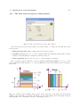
2. Second, select the quantities to be visualized ; they fall into two main groups: (1) sectional centers and
principal axes and (2) the warping, stress or strain fields over the cross-section. More details are given
in section 1.5.2.
3. Optionally, it is also possible to interactively define sensors as described in section 8.5, at specific
locations over the cross-section, as discussed in section 1.5.3.
The Graphics toolbar controls the manner in which the requested information is to be visualized, and
more details are given in section 1.5.4.
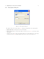
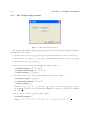
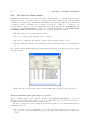
1.5.1
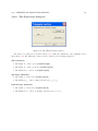
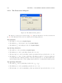
Step 1: Selecting a sectional loading case
The first step of the visualization phase is to select a sectional loading condition, as provided by the sectional
loads(see section 6.1). These user defined loading conditions form a list of loading conditions. The first three
entries or icons of the Loading menu shown in fig. 1.9 are used to navigate this loading list.
20
CHAPTER 1. INTRODUCTION
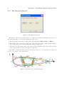
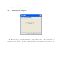
Figure 1.9: The Loading menu and toolbar. Each action can be invoked by selecting a menu item or clicking
the corresponding toolbar icon. In this figure, the menu items and corresponding toolbar icons are shown
next to each other to highlight the correspondence.
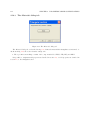
1. The Reference menu item or toolbar icon will show the reference configuration of the cross-section,
no loading condition is selected.
2. The First Loading menu item or toolbar icon activates the first loading condition in the list.
3. The Next Loading menu item or toolbar icon moves to the next loading condition in the list.
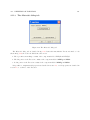
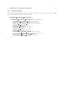
1.5.2
Step 2: Selecting the quantities to be visualized
The second step of the visualization phase is to select the quantities to be visualized. Nine entries or icons
in the Loading menu shown in fig. 1.9 are used to select the desired quantities to be visualized, and these
fall into two categories: (1) sectional centers and principal axes and, (2) the warping, stress or strain fields
over the cross-section.
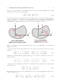
Visualizing centers and principal axes
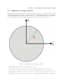
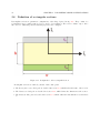
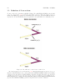
The first three entries or icons are used to visualize the centroid, shear center and center of mass of the
cross-section and the associated principal axes. These entries or icons are toggle switches that turn on and
off the visualization of the associated quantities. In all cases, the origin of the axis system, i.e. the reference
axis of the beam is indicated by a yellow circle.
1. The Princ. axes Bending menu item or toolbar icon switches on the visualization of the principal
centroidal axes of bending. The location of the centroid is given by eq. (1.17) and the orientation of
the principal centroidal axes by eq. (1.20), as illustrated in fig. 1.4. Examples are shown in fig. 2.10
and fig. 2.65.
2. The Princ. axes Shearing menu item or toolbar icon switches on the visualization of the principal
axes of shearing at the shear center. The location of the shear center is given by eq. (1.31) and the
1.5. VISUALIZING THE RESULTS
21
orientation of the principal axes of shearing at the shear center by eq. (1.34), as illustrated in fig. 1.6.
Examples are shown in fig. 2.16 and fig. 2.85.
3. The Princ. axes Inertia menu item or toolbar icon switches on the visualization of the principal
axes of inertia at the mass center. The location of the mass center is given by eq. (1.40) and the
orientation of the principal axes of inertia at the mass center by eq. (1.44), as illustrated in fig. 1.7.
Examples are shown in fig. 2.11 and fig. 2.79.
As discussed in section 1.4.1, the complete sectional stress-sectional strain relationship given by eq. (1.2) often
splits into an axial force-bending moment problem, characterized by eq. (1.5), and a twisting moment-shear
force problem, characterized by eq. (1.6). When this decoupling takes place, the Princ. axes Bending and
Princ. axes Shearing entries or icons will display the quantities indicated above. If the decoupling does
not take place, clicking these entries or icons will simply display the origin of the axis system, since the
corresponding centers and associated principal axes do not exist.
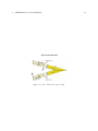
Visualizing warping, stress and strain fields
The next six entries or icons control the display of the warping displacement, stress and strain fields over the
cross-section. Clicking one of these entries or icons will cause the display of a specific displacement, stress
or strain component; the six actions are mutually exclusive.
1. Clicking the Displacements menu item or toolbar icon causes the display of the three-dimensional
warping displacement of the cross-section under the applied sectional loads. Examples are shown in
fig. 2.38 and fig. 2.78.
2. Clicking the Axial strains menu item or toolbar icon causes the display of the axial strain field over
the cross-section under the applied sectional loads. Examples are shown in fig. 2.44 and fig. 2.56.
3. Clicking the Shear strains menu item or toolbar icon causes the display of the shear strain field over
the cross-section under the applied sectional loads. Examples are shown in fig. 2.17 and fig. 2.29.
4. Clicking the Axial stresses menu item or toolbar icon causes the display of the axial stress field over
the cross-section under the applied sectional loads. Examples are shown in fig. 2.30, fig. 2.45, fig. 2.66
and fig. 2.92.
5. Clicking the Shear stresses menu item or toolbar icon causes the display of the shear stress field
over the cross-section under the applied sectional loads. Examples are shown in fig. 2.55 and fig. 2.73.
6. Clicking the Reserve Factors menu item or toolbar icon causes the display of the reserve factor field
over the cross-section under the applied sectional loads. When the menu item or toolbar icon Reserve
Factors is pressed, the reserve factors are computed over the cross-section, and the inverse of the
reserve factor is displayed. Examples are shown in fig. 2.72 and fig. 2.91.
The visualization of the centers and principal axes can be superimposed onto the display of these various
fields.
1.5.3
Step 3: Interactive definition of sensors
The last step of the visualization phase is the optional interactive definition of sensors. The last three entries
or icons of the Loading menu shown in fig. 1.9 are used to that effect; two options are possible: (1) a
temporary display the warping displacement, stress or strain levels at a point of the cross-section, or (2) the
interactive definition of sensors.
Temporary display of warping displacement, stress or strain levels
It is often important to obtain numerical, rather than graphical information about the warping displacement,
stress or strain levels at a point of the cross-section. This can be done by selecting a specific finite element
from the model, then displaying the stresses or strain at that point. The procedure is as follows.
22
CHAPTER 1. INTRODUCTION
1. Enter the visualization mode, select a loading condition, and visualize warping displacement, stress or
strain fields. These steps are described in sections 1.5.1 and 1.5.2.
2. To select an element of the finite element mesh, first click the Select Element menu item or toolbar
icon, then click on the desired element; that element will be highlighted as shown in fig. 1.10.
3. Next, click the Element Stresses menu item or toolbar icon to display the stresses or strain at the
center of the element. If the warping displacement, stress or strain field is presently visualized, warping
displacement, stress or strain levels will be displayed, respectively.
Fig. 1.10 illustrate this process while the shear stress field is visualized. An element of the mesh is selected,
and is highlighted, as shown on the figure. The temporary pop-up display gives the three-dimensional stress
components at the center point of the selected element. Once the OK icon is clicked, the box disappears, and
no record is kept of the stress level at that point. If a permanent record of the stress level is desired, the
interactive definition of a sensor should be used, as discussed in the next section.
Figure 1.10: The temporary display of stress levels.
Interactive definition of sensors
It is often convenient to create a permanent record of the warping displacement, stress or strain levels at
a point of the cross-section. This can be achieved through the interactive definition of sensors as described
in section 8.5, at specific locations of the cross-section. Once defined, these sensors become part of the
model definition and, as discussed in section 1.4.2, each time the finite element analysis is run, warping
displacements, stresses or strains will be output for each sensor and each loading condition.
To define a sensor, first select the desired element of the model, then create a sensor at that location.
The procedure is as follows.
1. Enter the visualization mode, select a loading condition, and visualize warping displacement, stress or
strain fields. These steps are described in sections 1.5.1 and 1.5.2.
2. To select an element of the finite element mesh, first click the Select Element menu item or toolbar
icon, then click on the desired element; that element will be highlighted as shown in fig.1.11.
1.5. VISUALIZING THE RESULTS
23
3. Next, click the Create Sensor menu item or toolbar icon to open the interactive sensor definition
dialog shown in fig.1.11 an fill in the following information.
(a) Sensor name. Enter a unique name for the sensor.
(b) Sensor type. Select Stresses, Strains or Warping for the sensor to compute the six stress
components, the six strain components, or the three warping components, respectively.
(c) Sensor Location. Select Middle, At Gauss Points or At Corners to locate one sensor at the
middle of the element, four sensors at each of the four Gauss points of the element, or four sensors
at the four corners of the element, respectively. For stresses and strains, the Gauss point option
provides the most accurate information, whereas for warping displacements, the four corner option
is preferable.
Figure 1.11: The interactive definition of a sensor.
1.5.4
The Graphics menu and toolbar
The Graphics menu and toolbar shown in fig. 1.12 controls the manner in which the requested information
is to be visualized.
1. The Zoom In and Zoom Out perform the familiar zoom in and zoom out function to focus on a specific
portion of the cross-section (zoom in), or obtain an overall view of the entire cross-section (zoom out).
2. The Center menu item or toolbar icon brings the geometric center of the cross-section to the center of
the graphical window, whereas the Show Model menu item or toolbar icon adjusts the zooming level
so the entire cross-section is visible in the graphical window.
3. Although a two-dimensional slice of beam is defined in the analysis, three-dimensional displacement,
stress, and strain fields are computed. To allow visualization of stress and strain components, it is
often necessary to rotate the model in the graphical window. The six entries or icons, Rotate X+,
Rotate X-, Rotate Y+, Rotate Y-, Rotate Z+ and Rotate Z- rotate the model by ±5 degrees about
the X, Y and Z axes, respectively. The X, Y and Z axes are screen axes.
24
CHAPTER 1. INTRODUCTION
4. Similarly, the four entries or icons, Translate X+, Translate X-, Translate Y+ and Translate Ytranslate the model by ±5% along the X or Y axes, respectively.
5. The View From X1 menu item or toolbar icon reset the view point so that the structural axis ı̄1 is now
perpendicular to the plane of the screen.
6. The size of the symbols used in the visualization can be adjusted using the Symbol size + or Symbol
size - entries or icons. The symbols are the circles used to indicate the locations of the sectional
centers and the arrays that represent the principal axes.
7. The size of the arrows used to visualize the strain or stress fields can be adjusted using the Data Size
+ or Data Size - entries or icons.
Figure 1.12: The Graphics menu and toolbar. Each action can be invoked by selecting a menu item or
clicking the corresponding toolbar icon. In this figure, the menu items and corresponding toolbar icons are
shown next to each other to highlight the correspondence..
1.6
1.6.1
Installation of SectionBuilder
Directory structure
A typical installation of the code features the following five sub-directories.
• SectionBuilder\bin. This directory contains the executable, SecBuild.exe and the input file icon
seb.ico.
1.6. INSTALLATION OF SECTIONBUILDER
25
• SectionBuilder\Demos. This directory contains a number of sample input files illustrating the various
types of cross-sections that can be defined.
• SectionBuilder\Manual. This directory contains the user’s manual in pdf format. The same document
can be found online manual
• SectionBuilder\Materials. This directory contains materials properties for a number of materials
in both international system of units and US units. These files should not be edited.
• SectionBuilder\Templates. This directory contains template files that should not be edited.
1.6.2
Input files
The following file types are input files for SectionBuilder.
• .sbf. These are input files to be executed by SectionBuilder. The input files contain the data in the
format described in this manual.
• .tpl. These are input files are template files that should not be edited.
1.6.3
Output files
The following file types are created by SectionBuilder and contain the results of the analysis.
• .bak. This file is backup file that duplicates the .seb input file.
• .html. This file echoes the definition of the model in hyper linked format.
• .out. This file echoes the definition of the cross-section and lists potential error and warning messages.
It can be viewed using any text editor.
• .sbp. This file contains the sectional stiffness and mass properties computed by SectionBuilder.
This file can be viewed using any text editor.
• .sbs. This file contains the three-dimensional warping displacements, stress components and strain
components computed by SectionBuilder for various loading cases. This file can be viewed using any
text editor.
• .sva. This file contains the information pertaining to the meshing of the cross-section. This file should
not be edited.
1.6.4
Installation Procedure
Follow the installation procedure for Windows XP.
1. Extract file SectionBuilder.rar to C:\.
2. Associate the extension .seb with the execution of the executable SectionBuilder\bin\SecBuild.exe.
From a folder’s window, click Tools->Folder Options. Once the Folder Options dialog is open, click
tab File Types. Click the New icon to Create New Extension dialog; type seb and click OK. With
the new file type seb highlighted in the Registered file types list, click Advanced to open the Edit
File Type dialog. Click Change icon then Browse and point to icon SectionBuilder\bin\seb.ico.
Next, click on New; type open under Action:, then click Browse and point to executable
SectionBuilder\bin\SecBuild.exe and click OK. Click OK and Close to exit the Folder Options
dialog.
3. Place a short cut to SectionBuilder\bin\SecBuild.exe on your desktop.
4. Verify the installation. Go to SectionBuilder\Demos\Airf and double click on airf1.seb; this should
open the SectionBuilder program.
26
CHAPTER 1. INTRODUCTION
Chapter 2
Parametric shape configurations
Parametric shape configurations have given geometric shapes that are parameterized. Parametric shape
configurations are defined through the Sections menu item shown in fig. 4.1 and can be of the following type:
airfoil sections as described in section 2.1, circular arcs as described in section 2.2, C-sections as described in
section 2.3, circular cylinders as described in section 2.4, double boxes as described in section 2.5, I-sections
as described in section 2.6, rectangular boxes as described in section 2.7, rectangular sections as described
in section 2.8, circular tubes as described in section 2.9, triangular sections as described in section 2.10, or
T-sections as described in section 2.11.
Figure 2.1: The section menu.
27
28
CHAPTER 2. PARAMETRIC SHAPE CONFIGURATIONS
2.1
Definition of airfoil sections
Airfoil sections are parametric configurations with no internal web, as depicted in fig. 2.2, or with one or
two internal webs, as shown in fig. 2.3 and 2.4, respectively. Airfoil sections consist of top and bottom
flanges with optional internal webs. The section consists of up to three zones to which independent material
properties can be assigned.
Figure 2.2: Configuration of the Airfoil Section with no web.
Figure 2.3: Configuration of the Airfoil Section with a single web.
Airfoil sections are defined by means of four dialog tabs.
1. The Airfoil-section dialog tab as described in section 2.1.1, which defines the name of the section.
2. The Airfoil profile dialog tab as described in section 2.1.2, which defines the outer geometry of the
section as a NACA four digit series airfoil.
3. The Dimensions dialog tab as described in section 2.1.3, which defines the dimensions of the section.
4. The Materials dialog tab as described in section 2.1.4, which defines the materials the section is made
of.
2.1. DEFINITION OF AIRFOIL SECTIONS
Figure 2.4: Configuration of the Airfoil Section with two webs.
29
30
CHAPTER 2. PARAMETRIC SHAPE CONFIGURATIONS
2.1.1
The Airfoil-section dialog tab
Figure 2.5: The Airfoil-section dialog tab.
The Airfoil-section dialog tab as described in fig. 2.5, defines the following data for the airfoil section.
1. Section name. Enter a unique name for the airfoil section.
2. Mesh density. Enter the desired mesh density as described in section 5.1, for the finite element
discretization.
3. (Defined in frame). The geometry of the airfoil section can be defined with respect to a fixed frame as
described in section 7.1, allowing translation and rotation of the section as a rigid body.
2.1. DEFINITION OF AIRFOIL SECTIONS
2.1.2
31
The Airfoil profile dialog tab
Figure 2.6: The Airfoil profile dialog tab.
The Airfoil profile dialog tab defines the outer aerodynamic profile for the airfoil section. This profile is
assumed to be one of the profiles defined by the NACA four digit series [1].
1. The first digit, 1, indicates the airfoil camber in percent of the chord (required input: integer
1 ∈ [0, 9]).
2. The second digit, 2, indicates the distance from the leading edge to the location of the maximum
camber, in tenth of the chord (required input: 2 ∈ [0, 9]).
3. The las two digits, 3, indicate the airfoil thickness in percent chord (required input: 3 ∈ [00, 09]).
For instance, the NACA 2415 airfoil section has 2 percent camber at 0.4 of the chord from the leading
edge and is 15 percent thick.
32
CHAPTER 2. PARAMETRIC SHAPE CONFIGURATIONS
2.1.3
The Dimensions dialog tab
Figure 2.7: The Dimensions dialog tab.
The Dimensions dialog tab as described in fig. 2.7, defines the dimensions of the airfoil section. The
section can feature no web as described in fig. 2.2, a single web as described in fig. 2.3, or two webs as
described in fig. 2.4. The dimensions of the section are defined by the following parameters.
Airfoil Dimensions
1. The chord, c, of the airfoil section (required input).
2. The thickness, tta1 , of the section wall for the no web design (required input). For the single or dual
web design, this is the wall thickness for the front portion of the airfoil.
Airfoil Thickness
1. The top wall thickness, tta2 , of the aft or middle portion of the airfoil for the single or dual web design,
respectively (default value: tta2 = tta1 ).
2. The bottom wall thickness, tba2 , of the aft or middle portion of the airfoil for the single or dual web
design, respectively (default value: tba2 = tta2 ).
3. The top wall thickness, tta3 , of the aft portion of the airfoil for the dual web design (default value:
tta3 = tta2 ).
4. The bottom wall thickness, tba3 , of the aft portion of the airfoil for the dual web design (default value:
tba3 = tta2 ).
Web 1 Dimensions
1. The location, xtw1 , of the intersection of the first web with the upper airfoil profile; this is a dimensional
quantity (default value: xtw1 = 0). This variable is also used as a flag for the presence of the first web:
if xtw1 6= 0, at least one web is present.
2. The location, xbw1 , of the intersection of the first web with the lower airfoil profile; this is a dimensional
quantity (default value: xbw1 = xtw1 ).
3. The thickness, tlw1 , of the left portion of the first web (default value: tlw1 = tta1 ).
4. The thickness, trw1 , of the right portion of the first web (default value: trw1 = tta2 ).
2.1. DEFINITION OF AIRFOIL SECTIONS
33
Web 2 Dimensions
1. The location, xtw2 , of the intersection of the second web with the upper airfoil profile; this is a
dimensional quantity (default value: xtw2 = 0). This variable is also used as a flag for the presence of
the second web: if xtw2 6= 0, two webs are present.
2. The location, xbw2 , of the intersection of the second web with the lower airfoil profile; this is a dimensional quantity (default value: xbw2 = xtw2 ).
3. The thickness, tlw2 , of the left portion of the second web (default value: tlw2 = tta1 ).
4. The thickness, trw2 , of the right portion of the second web (default value: trw2 = tta2 ).
34
CHAPTER 2. PARAMETRIC SHAPE CONFIGURATIONS
2.1.4
The Materials dialog tab
Figure 2.8: The Materials dialog tab.
The Materials dialog tab as described in fig. 2.8, defines the materials from which the airfoil section is
made. As shown in fig. 2.9, the section is divided into three zones.
1. The front portion of the airfoil consists of the components labeled Flg1U, Flg1L and LWeb1.
2. The middle portion of the airfoil consists of the components labeled RWeb1, Flg2U, Flg2L and LWeb2 ;
these components are present in the single and dual web designs only.
3. The aft portion of the airfoil consists of the components labeled RWeb2, Flg3U, Flg3L, TedU and TedL;
these components are present for the dual web design only.
It is possible to assign material properties as described in section 4.1, or solid properties as described in
section 4.2, to each zone of the airfoil section.
Figure 2.9: The three zones of the airfoil section.
2.1. DEFINITION OF AIRFOIL SECTIONS
2.1.5
35
Formatted input
The data that defines the airfoil section as described in the above sections will be saved in a specially formatted input file which has the following structure.
@AIRFOIL SECTION DEFINITION {
@AIRFOIL SECTION NAME { TboxName } {
@CHORD LENGTH { c }
@TOP AIRFOIL 1 THICKNESS { tta1 }
@NACA AIRFOIL PROFILE { 1, n2 , n3 }
@TOP AIRFOIL 2 THICKNESS { tta2 }
@BOTTOM AIRFOIL 2 THICKNESS { tba2 }
@TOP AIRFOIL 3 THICKNESS { tta3 }
@BOTTOM AIRFOIL 3 THICKNESS { tba3 }
@TOP WEB 1 LOCATION { ttw1 }
@BOTTOM WEB 1 LOCATION { tbw1 }
@LEFT WEB 1 THICKNESS { tlw1 }
@RIGHT WEB 1 THICKNESS { trw1 }
@TOP WEB 2 LOCATION { tta3 }
@BOTTOM WEB 2 LOCATION { tba3 }
@LEFT WEB 2 THICKNESS { tlw2 }
@RIGHT WEB 2 THICKNESS { trw2 }
@AIRFOIL 1 MATERIAL NAME { MaterialName1 }
@AIRFOIL 2 MATERIAL NAME { MaterialName2 }
@AIRFOIL 3 MATERIAL NAME { MaterialName3 }
@IS DEFINED IN FRAME { FxdFrameName }
@MESH DENSITY { md }
}
}
36
2.1.6
CHAPTER 2. PARAMETRIC SHAPE CONFIGURATIONS
Examples
A few examples that describe the construction procedure of this type of section are shown below.
Example 1
This example shows a NACA 4 digit series airfoil section. The chord length, thickness, material properties
and mesh density are assigned here. This example also shows the principal centroidal axes of bending.
Figure 2.10: Example 1-Airfoil Section.
Example 2
This example shows a NACA 4 digit series airfoil section. The section has 2 webs. The chord length, the
location of the webs, thickness of the upper, lower section and web, material properties and mesh density
are assigned here. This example also shows the principal axes of inertia at the mass center.
2.1. DEFINITION OF AIRFOIL SECTIONS
Figure 2.11: Example 2-Airfoil Section with Two Webs.
37
38
CHAPTER 2. PARAMETRIC SHAPE CONFIGURATIONS
2.2
Definition of circular arcs
Circular arcs are predefined sections presenting the shape shown in fig. 2.12. Circular arcs consist of an area
included between two circular arcs spanned by a common angle. The section consists of a single zone to
which material properties can be assigned. The circular arc is an open circular tube, as shown in fig. 2.12.
Closed circular tubes can be defined with the help of the circular tube predefined section as described in
section 2.9.
Figure 2.12: Configuration of the circular arc.
Circular arcs are defined by means of three dialog tabs.
1. The Circular Arc dialog tab as described in section 2.2.1, which defines the name of the section.
2. The Dimensions dialog tab as described in section 2.2.2, which defines the dimensions of the section.
3. The Materials dialog tab as described in section 2.2.3, which defines the materials the section is made
of.
2.2. DEFINITION OF CIRCULAR ARCS
2.2.1
39
The Circular Arc dialog tab
Figure 2.13: The Circular Arc dialog tab.
The Circular Arc dialog tab as described in fig. 2.13, defines the following data for the circular arc.
1. Section name. Enter a unique name for the circular arc.
2. Mesh density. Enter the desired mesh density as described in section 5.1, for the finite element
discretization.
3. (Defined in frame). The geometry of the circular arc can be defined with respect to a fixed frame as
described in section 7.1, allowing translation and rotation of the section as a rigid body.
40
CHAPTER 2. PARAMETRIC SHAPE CONFIGURATIONS
2.2.2
The Dimensions dialog tab
Figure 2.14: The Dimensions dialog tab.
The Dimensions dialog tab as described in fig. 2.14, defines the dimensions of the circular arc shown in
fig. 2.12. The dimensions of the section are defined by the following parameters.
1. The outer radius, RO , and inner radius, RI , of the circular tube (required input).
2. The initial angle, θI , and final angle, θF , of the circular arc, both measured in degrees (required
input). Note: 0 ≤ θI < 360, 0 < θF ≤ 360 and θI < θF . Even when θI = 0 and θF = 360, the circular
arc is still an open circular tube.
2.2. DEFINITION OF CIRCULAR ARCS
2.2.3
41
The Materials dialog tab
Figure 2.15: The Materials dialog tab.
The Materials dialog tab as described in fig. 2.15, defines the materials the circular arc is made of. As
shown in fig. 2.12, the section consists of a single zone to which it is possible to assign material properties
as described in section 4.1, or solid properties as described in section 4.2.
42
CHAPTER 2. PARAMETRIC SHAPE CONFIGURATIONS
2.2.4
Formatted input
The data that defines the circular arc as described in the above sections will be saved in a specially formatted
input file which has the following structure.
@CIRCULAR ARC DEFINITION {
@CIRCULAR ARC NAME { TboxName } {
@INNER RADIUS { RI }
@OUTER RADIUS { RO }
@THETA INITIAL { θI }
@THETA FINAL { θF }
@MATERIAL PROPERTY NAME { MaterialName }
@IS DEFINED IN FRAME { FxdFrameName }
@MESH DENSITY { md }
}
}
2.2. DEFINITION OF CIRCULAR ARCS
2.2.5
43
Examples
A few examples that describe the construction procedure of this type of section are shown below.
Example 1
This example shows a circular arc. Here the inner and outer radii, initial (0 degree) and final (180
degrees) angular positions of the arc, material and mesh density are assigned for constructing this section.
This example also shows the principal axes of shearing at the shear center.
Figure 2.16: Example 2-Circular Arc Section.
Example 2
This example shows a circular arc. Here the inner and outer radii, initial and final angular positions of
the arc, material and mesh density are assigned for constructing this section. This example also shows the
shear strain field over the cross-section under the applied sectional loads.
44
CHAPTER 2. PARAMETRIC SHAPE CONFIGURATIONS
Figure 2.17: Example 2-Circular Arc Section.
2.3. DEFINITION OF C-SECTIONS
2.3
45
Definition of C-sections
C-sections are parametric configurations of the shape depicted in fig. 2.18. They consist of a C-section,
possibly reinforced by top and/or bottom flanges. The section consists of up to three zones to which
independent material properties can be assigned. Note that through the use of fixed frames as described in
section 7.1, the C-section can be made to look like the following shapes: u, t, <, or =.
Figure 2.18: Configuration of the C-section.
C-sections are defined by means of three dialog tabs.
1. The C-section dialog tab as described in section 2.3.1, which defines the name of the section.
2. The Dimensions dialog tab as described in section 2.3.2, which defines the dimensions of the section.
3. The Materials dialog tab as described in section 2.3.3, which defines the materials the section is made
of.
46
CHAPTER 2. PARAMETRIC SHAPE CONFIGURATIONS
2.3.1
The C-section dialog tab
Figure 2.19: The C-section dialog tab.
The C-section dialog tab as described in fig. 2.19, defines the following data for the C-section.
1. Section name. Enter a unique name for the C-section.
2. Mesh density. Enter the desired mesh density as described in section 5.1, for the finite element
discretization.
3. (Defined in frame). The geometry of the C-section can be defined with respect to a fixed frame as
described in section 7.1, allowing translation and rotation of the section as a rigid body.
2.3. DEFINITION OF C-SECTIONS
2.3.2
47
The Dimensions dialog tab
Figure 2.20: The Dimensions dialog tab.
The Dimensions dialog tab as described in fig. 2.20, defines the dimensions of the C-section, as depicted
in fig. 2.18. The dimensions of the section are defined by the following parameters.
Web dimensions
1. The height, h, of the web (required input).
2. The thickness, tw , of the web (required input).
Top flange dimensions
1. The width, wtf , of the top flange(required input).
2. The thickness, ttf , of the top flange (default value: ttf = tw ).
3. The skew angle, αtf , of the top flange, positive up, measured in degrees (default value: αtf = 0).
4. The thickness, ttr , of the top reinforcement flange; this thickness applies to both left and right reinforcements, which cannot exist independently of each other (default value: ttr = 0). This variable is
also used as a flag for the presence of the top flange reinforcement: if ttr > 0, this reinforcement is
present.
Bottom flange dimensions
1. The width, wbf , of the bottom flange(default value: wbf = wtf ).
2. The thickness, tbf , of the bottom flange (default value: tbf = ttf ).
3. The skew angle, αbf , of the top flange, positive down, measured in degrees (default value: αbf = 0).
4. The thickness, tbr , of the bottom reinforcement flange; this thickness applies to both left and right
reinforcements, which cannot exist independently of each other (default value: tbr = 0). This variable
is also used as a flag for the presence of the bottom flange reinforcement: if tbr > 0, this reinforcement
is present.
48
CHAPTER 2. PARAMETRIC SHAPE CONFIGURATIONS
2.3.3
The Materials dialog tab
Figure 2.21: The Materials dialog tab.
The Materials dialog tab as described in fig. 2.21, defines the materials the C-section is made of. As
shown in fig. 2.22, the section is divided into three zones.
1. The top reinforcement flange consists of a single solid labeled TFlgR.
2. The C-section it self consists of the solids labeled TFlg, Web, BFlg.
3. The bottom reinforcement flange consists of a single solid labeled BFlgR.
It is possible to assign material properties as described in section 4.1, or solid properties as described in
section 4.2, to each zone of the C-section.
Special Cases
1. If the width, wtf = 0, the section looks like L-shape depicted in fig. 2.23. This L-shape section does
not have TFlgR and TFlg solids shown in fig. 2.24.
2. If the width, wbf = 0, the section looks like reverse L-shape depicted in fig. 2.25. This reverse L-shape
section does not have BFlgR and BFlg solids shown in fig. 2.26.
3. If the widths, wtf = 0 and wbf = 0, the section looks like a strip depicted in fig. 2.27. This strip section
does not have TFlgR, TFlg, BFlgR and BFlg solids shown in fig. 2.28. It only has Web.
2.3. DEFINITION OF C-SECTIONS
Figure 2.22: The three zones of the C-section.
49
50
CHAPTER 2. PARAMETRIC SHAPE CONFIGURATIONS
Figure 2.23: Configuration of the L-section.
2.3. DEFINITION OF C-SECTIONS
Figure 2.24: The two zones of the L-section.
51
52
CHAPTER 2. PARAMETRIC SHAPE CONFIGURATIONS
Figure 2.25: Configuration of the reverse L-section.
2.3. DEFINITION OF C-SECTIONS
Figure 2.26: The two zones of the reverse L-section.
53
54
CHAPTER 2. PARAMETRIC SHAPE CONFIGURATIONS
Figure 2.27: Configuration of the strip section.
2.3. DEFINITION OF C-SECTIONS
Figure 2.28: The zone of the strip section.
55
56
CHAPTER 2. PARAMETRIC SHAPE CONFIGURATIONS
2.3.4
Formatted input
The data that defines the C-section as described in the above sections will be saved in a specially formatted
input file which has the following structure.
@C SECTION DEFINITION {
@C SECTION NAME { CsecName } {
@WEB HEIGHT { h }
@WEB THICKNESS { tw }
@TOP FLANGE WIDTH { wtf }
@TOP FLANGE THICKNESS { ttf }
@TOP FLANGE SKEW ANGLE { αtf }
@TOP FLANGE REINFORCE THICKNESS { ttr }
@BOTTOM FLANGE WIDTH { wbf }
@BOTTOM FLANGE THICKNESS { tbf }
@BOTTOM FLANGE SKEW ANGLE { αbf }
@BOTTOM FLANGE REINFORCE THICKNESS { tbr }
@WEB MATERIAL NAME { WebMaterialName }
@TOP REINFORCE MATERIAL NAME { TopMaterialName }
@BOTTOM REINFORCE MATERIAL NAME { BottomMaterialName }
@IS DEFINED IN FRAME { FxdFrameName }
@MESH DENSITY { md }
}
}
2.3. DEFINITION OF C-SECTIONS
2.3.5
57
Examples
A few examples that describe the construction procedure of this type of section are shown below.
Example 1
This example shows a C-section. Here web height, web thickness, top flange width, web material and
mesh density are assigned for constructing this section. This example also shows the shear strain field over
the cross-section under the applied sectional loads.
Figure 2.29: Example 1.C-Section
Example 2
This example shows also a C-section with skewed top and bottom flanges. Here web height, web thickness,
top flange width, top flange thickness, flange reinforce thicknesses, flange skew angles, materials and mesh
density are assigned for constructing this section. This example also shows the axial stress field over the
cross-section under the applied sectional loads.
Example 3
This example shows a reverse L-section. Here web height, web thickness, top flange width, bottom flange
width=0, web material and mesh density are assigned for constructing this section. This example also shows
principal centroidal axes of bending.
Example 4
This example shows a L-section. Here web height, web thickness, top flange width=0, bottom flange
width, flange reinforce thickness, materials and mesh density are assigned for constructing this section. This
example also shows axial stress field over the cross-section under the applied sectional loads.
Example 5
This example shows a strip section. Here web height, web thickness, top flange width = 0, bottom flange
width=0, web material and mesh density are assigned for constructing this section. This example also shows
principal axes of inertia at the mass center.
58
CHAPTER 2. PARAMETRIC SHAPE CONFIGURATIONS
Figure 2.30: Example 2.C-Section
Figure 2.31: Example 3.Reverse L-Section
2.3. DEFINITION OF C-SECTIONS
Figure 2.32: Example 4. L-Section
Figure 2.33: Example 5.Strip Section
59
60
CHAPTER 2. PARAMETRIC SHAPE CONFIGURATIONS
2.4
Definition of circular cylinders
Circular cylinders are predefined sections presenting the shape shown in fig. 2.34. Circular cylinders consist
of a solid circular cylinder. The section consists of a single zone to which material properties can be assigned.
The circular cylinders are solid cylinders, as shown in fig. 2.34. Hollow circular cylinder, or circular tubes
can be defined with the help of the circular tube predefined section as described in section 2.9.
Figure 2.34: Configuration of the circular cylinder.
Circular cylinders are defined by means of three dialog tabs.
1. The Cylinder dialog tab as described in section 2.4.1, which defines the name of the section.
2. The Dimensions dialog tab as described in section 2.4.2, which defines the dimensions of the section.
3. The Materials dialog tab as described in section 2.4.3, which defines the materials the section is made
of.
2.4. DEFINITION OF CIRCULAR CYLINDERS
2.4.1
61
The Cylinder dialog tab
Figure 2.35: The Cylinder dialog tab.
The Cylinder dialog tab as described in fig. 2.35, defines the following data for the circular cylinder.
1. Section name. Enter a unique name for the circular cylinder.
2. Mesh density. Enter the desired mesh density as described in section 5.1, for the finite element
discretization.
3. (Defined in frame). The geometry of the circular cylinder can be defined with respect to a fixed frame
as described in section 7.1, allowing translation and rotation of the section as a rigid body.
62
CHAPTER 2. PARAMETRIC SHAPE CONFIGURATIONS
2.4.2
The Dimensions dialog tab
Figure 2.36: The Dimensions dialog tab.
The Dimensions dialog tab defines the dimensions of the circular cylinder shown in fig. 2.34. The
dimensions of the section are defined by a single parameter.
1. The radius, R of the cylinder (required input).
2.4. DEFINITION OF CIRCULAR CYLINDERS
2.4.3
63
The Materials dialog tab
Figure 2.37: The Materials dialog tab.
The Materials dialog tab defines the materials the circular cylinder is made of. The section is made of a
single, homogeneous material. It is possible to assign material properties as described in section 4.1, to the
section.
64
CHAPTER 2. PARAMETRIC SHAPE CONFIGURATIONS
2.4.4
Formatted input
The data defined in the above sections will be saved in a specially formatted input file which has the following
structure.
@CYLINDER DEFINITION {
@CYLINDER NAME { CyldName } {
@RADIUS { R }
@MATERIAL PROPERTY NAME { MaterialName }
@IS DEFINED IN FRAME { FxdFrameName }
@MESH DENSITY { md }
}
}
2.4. DEFINITION OF CIRCULAR CYLINDERS
2.4.5
65
Examples
An example that describes the construction procedure of this type of section is shown below.
Example 1
This example shows a Circular cylinder. Here radius, frame definition, material and mesh density are
assigned for constructing this section. This example also shows the warping displacement of the cross-section
under the applied sectional loads.
Figure 2.38: Example 1-Cylinder.
66
CHAPTER 2. PARAMETRIC SHAPE CONFIGURATIONS
2.5
Definition of double boxes
Double boxes are parametric configurations of the shape depicted in fig. 2.39. They consist of an double
box, possibly reinforced by top and/or bottom flanges. The section consists of up to four zones to which
independent material properties can be assigned. Note that through the use of fixed frames as described in
section 7.1, the double box can be made to look like the following shapes: H-sections.
Figure 2.39: Configuration of the double box.
Double boxes are defined by means of three dialog tabs.
1. The Double Box dialog tab as described in section 2.5.1, which defines the name of the section.
2. The Dimensions dialog tab as described in section 2.5.2, which defines the dimensions of the section.
3. The Materials dialog tab as described in section 2.5.3, which defines the materials the section is made
of.
2.5. DEFINITION OF DOUBLE BOXES
2.5.1
67
The Double Box dialog tab
Figure 2.40: The Double Box dialog tab.
The Double Box dialog tab as described in fig. 2.40, defines the following data for the double box.
1. Section name. Enter a unique name for the double box.
2. Mesh density. Enter the desired mesh density as described in section 5.1, for the finite element
discretization.
3. (Defined in frame). The geometry of the double box can be defined with respect to a fixed frame as
described in section 7.1, allowing translation and rotation of the section as a rigid body.
68
CHAPTER 2. PARAMETRIC SHAPE CONFIGURATIONS
2.5.2
The Dimensions dialog tab
Figure 2.41: The Dimensions dialog tab.
The Dimensions dialog tab as described in fig. 2.5.2, defines the dimensions of the double box shown in
fig. 2.39. The dimensions of the section are defined by the following parameters.
Web dimensions
1. The height, h, of the section (required input).
2. The thickness, tlw , of the left part of the web (required input).
3. The thickness, trw , of the right part of the web (required input).
Top left flange dimensions
1. The width, wtlf , of the top left flange (required input).
2. The thickness, ttlf , of the top left flange (default value: ttlf = tlw ).
3. The skew angle, αtlf , of the top left flange, positive up, measured in degrees (default value: αtlf = 0).
4. The thickness, ttr , of the top reinforcement flange; this thickness applies to both left and right reinforcements that cannot exist independently of each other (default value: ttr = 0). This variable is also
used as a flag for the presence of the top flange reinforcement: if ttr > 0, this reinforcement is present.
Top right flange dimensions
1. The width, wtrf , of the top right flange (default value: wtrf = wtlf ).
2. The thickness, ttrf , of the top right flange (default value: ttrf = trw ).
3. The skew angle, αtrf , of the top right flange, positive up, measured in degrees (default value: αtrf = 0).
Bottom left flange dimensions
1. The width, wblf , of the bottom left flange (default value: wblf = wtlf ).
2. The thickness, tblf , of the bottom left flange (default value: tblf = ttlf ).
3. The skew angle, αblf , of the bottom left flange, positive down, measured in degrees (default value:
αblf = 0).
2.5. DEFINITION OF DOUBLE BOXES
69
4. The thickness, tbr , of the bottom reinforcement flange; this thickness applied to both left and right
reinforcements that cannot exist independently of each other (default value: tbr = 0). This variable is
also used as a flag for the presence of the bottom flange reinforcement: if tbr > 0, this reinforcement is
present.
Bottom right flange dimensions
1. The width, wbrf , of the bottom right flange (default value: wbrf = wtrf ).
2. The thickness, tbrf , of the bottom right flange (default value: tbrf = ttrf ).
3. The skew angle, αbrf , of the bottom right flange, positive down, measured in degrees (default value:
αbrf = 0).
70
CHAPTER 2. PARAMETRIC SHAPE CONFIGURATIONS
2.5.3
The Materials dialog tab
Figure 2.42: The Materials dialog tab.
The Materials dialog tab as described in fig. 2.42, defines the materials the double box is made of. As
shown in fig. 2.43, the section is divided into four zones.
1. The top reinforcement flange consists of components labeled TLFlgR and TRFlgR
2. The left portion of the double box itself consists of components labeled TLFlg, LWeb and BLFlg.
3. The right portion of the double box itself consists of components labeled TRFlg, RWeb and BRFlg.
4. The top reinforcement flange consists of components labeled BLFlgR and BRFlgR.
It is possible to assign material properties as described in section 4.1, or solid properties as described in
section 4.2, to each zone of the double box.
2.5. DEFINITION OF DOUBLE BOXES
Figure 2.43: The four zones of the double box.
71
72
CHAPTER 2. PARAMETRIC SHAPE CONFIGURATIONS
2.5.4
Formatted input
The data defined in the above sections will be saved in a specially formatted input file which has the following
structure.
@DOUBLE BOX DEFINITION {
@DOUBLE BOX NAME { DboxName } {
@WEB HEIGHT { h }
@LEFT WEB THICKNESS { tlw }
@RIGHT WEB THICKNESS { trw }
@TOP FLANGE WIDTH { wtf }
@TOP FLANGE THICKNESS { ttf }
@TOP FLANGE SKEW ANGLE { αtf }
@TOP FLANGE REINFORCE THICKNESS { ttr }
@BOTTOM FLANGE WIDTH { wbf }
@BOTTOM FLANGE THICKNESS { tbf }
@BOTTOM FLANGE SKEW ANGLE { αbf }
@BOTTOM FLANGE REINFORCE THICKNESS { tbr }
@LEFT WEB MATERIAL NAME { LWebMaterialName }
@RIGHT WEB MATERIAL NAME { RWebMaterialName }
@TOP REINFORCE MATERIAL NAME { TopMaterialName }
@BOTTOM REINFORCE MATERIAL NAME { BottomMaterialName }
@IS DEFINED IN FRAME { FxdFrameName }
@MESH DENSITY { md }
}
}
2.5.5
Examples
A few examples that describe the construction procedure of this type of section are shown below.
Example 1
This example shows a double box. Here web height, web thicknesses, flange width, web materials and
mesh density are assigned for constructing this section. This example also shows the axial strain field over
the cross-section under the applied sectional loads.
Example 2
This example shows a double box with skewed flanges. Here web height, web thicknesses, flange
widths,flange thicknesses, flange reinforcement thickness, flange skew angles, materials and mesh density
are assigned for constructing this section. This example also shows the axial stress field over the crosssection under the applied sectional loads.
2.5. DEFINITION OF DOUBLE BOXES
Figure 2.44: Example 1-Double Box.
Figure 2.45: Example 2-Double Box.
73
74
CHAPTER 2. PARAMETRIC SHAPE CONFIGURATIONS
2.6
Definition of I-sections
I-sections are parametric configurations of the shape depicted in fig. 2.46. They consist of an I-section, possibly reinforced by top and/or bottom flanges. The section consists of up to four zones to which independent
material properties can be assigned. Note that through the use of fixed frames as described in section 7.1,
the I-section can be made to look like the following shapes: H-sections.
Figure 2.46: Configuration of the I-section.
I-sections are defined by means of three dialog tabs.
1. The I-section dialog tab as described in section 2.6.1, which defines the name of the section.
2. The Dimensions dialog tab as described in section 2.6.2, which defines the dimensions of the section.
3. The Materials dialog tab as described in section 2.6.3, which defines the materials the section is made
of.
2.6. DEFINITION OF I-SECTIONS
2.6.1
75
The I-section dialog tab
Figure 2.47: The I-section dialog tab.
The I-section dialog tab as described in fig. 2.47, defines the following data for the I-section.
1. Section name. Enter a unique name for the I-section.
2. Mesh density. Enter the desired mesh density as described in section 5.1, for the finite element
discretization.
3. (Defined in frame). The geometry of the I-section can be defined with respect to a fixed frame as
described in section 7.1, allowing translation and rotation of the section as a rigid body.
76
CHAPTER 2. PARAMETRIC SHAPE CONFIGURATIONS
2.6.2
The Dimensions dialog tab
Figure 2.48: The Dimensions dialog tab.
The Dimensions dialog tab as described in fig. 2.6.2, defines the dimensions of the I-section shown in
fig. 2.46. The dimensions of the section are defined by the following parameters.
Web dimensions
1. The height, h, of the section (required input).
2. The thickness, tlw , of the left part of the web (required input).
3. The thickness, trw , of the right part of the web (required input).
Top left flange dimensions
1. The width, wtlf , of the top left flange (required input).
2. The thickness, ttlf , of the top left flange (default value: ttlf = tlw ).
3. The skew angle, αtlf , of the top left flange, positive up, measured in degrees (default value: αtlf = 0).
4. The thickness, ttr , of the top reinforcement flange; this thickness applies to both left and right reinforcements that cannot exist independently of each other (default value: ttr = 0). This variable is also
used as a flag for the presence of the top flange reinforcement: if ttr > 0, this reinforcement is present.
Top right flange dimensions
1. The width, wtrf , of the top right flange (default value: wtrf = wtlf ).
2. The thickness, ttrf , of the top right flange (default value: ttrf = trw ).
3. The skew angle, αtrf , of the top right flange, positive up, measured in degrees (default value: αtrf = 0).
Bottom left flange dimensions
1. The width, wblf , of the bottom left flange (default value: wblf = wtlf ).
2. The thickness, tblf , of the bottom left flange (default value: tblf = ttlf ).
3. The skew angle, αblf , of the bottom left flange, positive down, measured in degrees (default value:
αblf = 0).
2.6. DEFINITION OF I-SECTIONS
77
4. The thickness, tbr , of the bottom reinforcement flange; this thickness applied to both left and right
reinforcements that cannot exist independently of each other (default value: tbr = 0). This variable is
also used as a flag for the presence of the bottom flange reinforcement: if tbr > 0, this reinforcement is
present.
Bottom right flange dimensions
1. The width, wbrf , of the bottom right flange (default value: wbrf = wtrf ).
2. The thickness, tbrf , of the bottom right flange (default value: tbrf = ttrf ).
3. The skew angle, αbrf , of the bottom right flange, positive down, measured in degrees (default value:
αbrf = 0).
78
CHAPTER 2. PARAMETRIC SHAPE CONFIGURATIONS
2.6.3
The Materials dialog tab
Figure 2.49: The Materials dialog tab.
The Materials dialog tab as described in fig. 2.49, defines the materials the I-section is made of. As
shown in fig. 2.50, the section is divided into four zones.
1. The top reinforcement flange consists of components labeled TLFlgR and TRFlgR
2. The left portion of the I-section itself consists of components labeled TLFlg, LWeb and BLFlg.
3. The right portion of the I-section itself consists of components labeled TRFlg, RWeb and BRFlg.
4. The top reinforcement flange consists of components labeled BLFlgR and BRFlgR.
It is possible to assign material properties as described in section 4.1, or solid properties as described in
section 4.2, to each zone of the I-section.
Special Cases
1. If the widths, wtrf = 0 and wblf = 0, the section looks like Z-shape depicted in fig. 2.51. This Z-section
does not have TRFlgR, TRFlg, BLFlgR and BLFlg solids shown in fig. 2.52. Here the coordinates of
the points are also adjusted from the I-section.
2. If the widths, wblf = 0 and wbrf = 0, the section looks like T-shape depicted in fig. 2.53. This T-section
does not have BLFlgR, BLFlg, BRFlgR, and BRFlg solids shown in fig. 2.54. Here the coordinates of
the points are also adjusted from the I-section.
2.6. DEFINITION OF I-SECTIONS
Figure 2.50: The four zones of the I-Section.
79
80
CHAPTER 2. PARAMETRIC SHAPE CONFIGURATIONS
Figure 2.51: Configuration of the Z-section.
2.6. DEFINITION OF I-SECTIONS
Figure 2.52: The zones of the Z-section.
81
82
CHAPTER 2. PARAMETRIC SHAPE CONFIGURATIONS
Figure 2.53: Configuration of the T-section.
2.6. DEFINITION OF I-SECTIONS
Figure 2.54: The zones of the T-section.
83
84
CHAPTER 2. PARAMETRIC SHAPE CONFIGURATIONS
2.6.4
Formatted input
The data defined in the above sections will be saved in a specially formatted input file which has the following
structure.
@I SECTION DEFINITION {
@I SECTION NAME { IsecName } {
@WEB HEIGHT { h }
@LEFT WEB THICKNESS { tlw }
@RIGHT WEB THICKNESS { trw }
@TOP FLANGE WIDTH { wtf }
@TOP FLANGE THICKNESS { ttf }
@TOP FLANGE SKEW ANGLE { αtf }
@TOP FLANGE REINFORCE THICKNESS { ttr }
@BOTTOM FLANGE WIDTH { wbf }
@BOTTOM FLANGE THICKNESS { tbf }
@BOTTOM FLANGE SKEW ANGLE { αbf }
@BOTTOM FLANGE REINFORCE THICKNESS { tbr }
@LEFT WEB MATERIAL NAME { LWebMaterialName }
@RIGHT WEB MATERIAL NAME { RWebMaterialName }
@TOP REINFORCE MATERIAL NAME { TopMaterialName }
@BOTTOM REINFORCE MATERIAL NAME { BottomMaterialName }
@IS DEFINED IN FRAME { FxdFrameName }
@MESH DENSITY { md }
}
}
2.6.5
Examples
A few examples that describe the construction procedure of this type of section are shown below.
Example 1
This example shows an I-section. Here web height, web thicknesses, flange widths, flange thicknesses,
web materials and mesh density are assigned for constructing this section. This example also shows the
shear stress field over the cross-section under the applied sectional loads.
Example 2
This example shows an I-section with top and bottom reinforcements. Here web height, web thicknesses,
flange widths, flange reinforcement thicknesses, materials and mesh density are assigned for constructing
this section. This example also shows the axial strain field over the cross-section under the applied sectional
loads.
Example 3
This example also shows a Z-section without any reinforcement. Here web height, web thicknesses, flange
widths (here wtrf = 0 and wblf = 0), materials and mesh density are assigned for constructing this section.
This example also shows principal centroidal axes of bending.
Example 4
This example shows a Z-section with top and bottom reinforcements. Here web height, web thicknesses,
flange widths (here wtrf = 0 and wblf = 0), flange reinforcement thicknesses, materials and mesh density are
2.6. DEFINITION OF I-SECTIONS
85
Figure 2.55: Example 1.I-section
assigned for constructing this section. This example also shows the axial stress field over the cross-section
under the applied sectional loads.
Example 5
This example shows a T-section with top reinforcement. Here web height, web thicknesses, flange widths
(here wblf = 0 and wbrf = 0), flange reinforcement thicknesses, materials and mesh density are assigned for
constructing this section. This example also shows the principal axes of inertia at the mass center.
86
CHAPTER 2. PARAMETRIC SHAPE CONFIGURATIONS
Figure 2.56: Example 2.I-section
Figure 2.57: Example 3.Z-section
2.6. DEFINITION OF I-SECTIONS
Figure 2.58: Example 4.Z-section
Figure 2.59: Example 5.T-section
87
88
CHAPTER 2. PARAMETRIC SHAPE CONFIGURATIONS
2.7
Definition of rectangular boxes
Rectangular boxes are parametric configurations of the shape depicted in fig. 2.60. They consist of a rectangular box, possibly reinforced by top and/or bottom flanges. The section consists of up to three three zones
to which independent material properties can be assigned.
Figure 2.60: Configuration of the rectangular box. The dimensions of the various elements of the section are
indicated on the figure. The three shaded areas correspond to the three zones of three section.
Rectangular boxes are defined by means of three dialog tabs.
1. The Rectangular box dialog tab as described in section 2.7.1, which defines the name of the section.
2. The Dimensions dialog tab as described in section 2.7.2, which defines the dimensions of the section.
3. The Materials dialog tab as described in section 2.7.3, which defines the materials the section is made
of.
2.7. DEFINITION OF RECTANGULAR BOXES
2.7.1
89
The Rectangular box dialog tab
Figure 2.61: The Rectangular box dialog tab.
The Rectangular box dialog tab as described in fig. 2.61, defines the following data for the rectangular
box.
1. Section name. Enter a unique name for the rectangular box.
2. Mesh density. Enter the desired mesh density as described in section 5.1, for the finite element
discretization.
3. (Defined in frame). The geometry of the rectangular box can be defined with respect to a fixed frame
as described in section 7.1, allowing translation and rotation of the section as a rigid body.
90
CHAPTER 2. PARAMETRIC SHAPE CONFIGURATIONS
2.7.2
The Dimensions dialog tab
Figure 2.62: The Dimensions dialog tab.
The Dimensions dialog tab as described in fig. 2.62, defines the dimensions of the rectangular box, as
depicted in fig. 2.60. Dimensions of the section are defined by the following parameters.
Web dimensions
1. The height, h, of the section (required input).
2. The thickness, tlw , of the left web (required input).
3. The thickness, trw , of the right web (required input).
Top left flange dimensions
1. The width, wtlf , of the top left flange (required input).
2. The thickness, ttf , of the top flange (default value: ttf = tlw ).
3. The skew angle, αtlf , of the top left flange, positive up, measured in degrees (default value: αtlf = 0).
4. The thickness, ttr , of the top reinforcement flange; this thickness applies to both left and right reinforcements that cannot exist independently of each other (default value: ttr = 0). This variable is also
used as a flag for the presence of the top reinforcement flange: if ttr 6= 0, the top reinforcement flange
is present.
Top right flange dimensions
1. The width, wtrf , of the top right flange (default value: wtrf = wtlf ).
2. The thickness of the top right flange equals that of the top left flange.
3. The skew angle, αtrf , of the top right flange, positive up, measured in degrees (default value: αtrf = 0).
Bottom left flange dimensions
1. The width, wblf , of the bottom left flange (default value: wblf = wtlf ).
2. The thickness, tbf , of the bottom left flange (default value: tbf = ttf ).
2.7. DEFINITION OF RECTANGULAR BOXES
91
3. The skew angle, αblf , of the bottom left flange, positive down, measured in degrees (default value:
αblf = 0).
4. The thickness, tbr , of the bottom reinforcement flange; this thickness applied to both left and right
reinforcements that cannot exist independently of each other (default value: tbr = 0). This variable
is also used as a flag for the presence of the bottom reinforcement flange: if tbr 6= 0, the bottom
reinforcement flange is present.
Bottom right flange dimensions
1. The width, wbrf , of the bottom right flange (default value: wbrf = wblf ).
2. The thickness of the bottom right flange equals that of the bottom left flange.
3. The skew angle, αbrf , of the bottom right flange, positive down, measured in degrees (default value:
αbrf = 0).
92
CHAPTER 2. PARAMETRIC SHAPE CONFIGURATIONS
2.7.3
The Materials dialog tab
Figure 2.63: The Materials dialog tab.
The Materials dialog tab as described in fig. 2.63, defines the materials the rectangular box is made of.
As shown in fig. 2.64, the section is divided into three zones.
1. The top reinforcement flange consists of the components labeled TLFlgR and TRFlgR.
2. The rectangular box consists of the components labeled TLFlg, TRFlg, LWeb, RWeb, BLFlg, and
BRFlg.
3. The bottom reinforcement flange consists of the components labeled BLFlgR and BRFlgR.
It is possible to assign material properties as described in section 4.1, or solid properties as described in
section 4.2, to each zone of the rectangular box.
2.7. DEFINITION OF RECTANGULAR BOXES
Figure 2.64: The three zones of the rectangular box.
93
94
CHAPTER 2. PARAMETRIC SHAPE CONFIGURATIONS
2.7.4
Formatted input
The data that defines the rectangular box as described in the above sections will be saved in a specially
formatted input file which has the following structure.
@RECTANGULAR BOX DEFINITION {
@RECTANGULAR BOX NAME { RBoxName } {
@HEIGHT { h }
@LEFT WEB THICKNESS { tlw }
@RIGHT WEB THICKNESS { trw }
@TOP LEFT FLANGE WIDTH { wtlf }
@TOP LEFT FLANGE THICKNESS { ttf }
@TOP LEFT FLANGE SKEW ANGLE { αtlf }
@TOP FLANGE REINFORCE THICKNESS { ttr }
@TOP RIGHT FLANGE WIDTH { wtrf }
@TOP RIGHT FLANGE SKEW ANGLE { αtrf }
@BOTTOM LEFT FLANGE WIDTH { wblf }
@BOTTOM LEFT FLANGE THICKNESS { tbf }
@BOTTOM LEFT FLANGE SKEW ANGLE { αblf }
@BOTTOM FLANGE REINFORCE THICKNESS { tbr }
@BOTTOM RIGHT FLANGE WIDTH { wbrf }
@BOTTOM RIGHT FLANGE SKEW ANGLE { αbrf }
@WEB MATERIAL NAME { WebMaterialName }
@TOP REINFORCE MATERIAL NAME { TopMaterialName }
@BOTTOM REINFORCE MATERIAL NAME { BottomMaterialName }
@IS DEFINED IN FRAME { FxdFrameName }
@MESH DENSITY { md }
}
}
2.7.5
Examples
A few examples that describe the construction procedure of this type of section are shown below.
Example 1
This example shows a rectangular box with skewed flanges. Here height, web thicknesses, flange widths,
flange skew angles, materials and mesh density are assigned for constructing this section.This example also
shows the principal centroidal axes of bending.
Example 2
This example shows a rectangular box with top and bottom flange reinforcements. Here height, web
thicknesses, flange widths, flange thickness, bottom left flange skew angle, materials and mesh density are
assigned for constructing this section. This example also shows the axial stress field over the cross-section
under the applied sectional loads.
2.7. DEFINITION OF RECTANGULAR BOXES
Figure 2.65: Example 1-Rectangular Box.
Figure 2.66: Example 2-Rectangular Box.
95
96
CHAPTER 2. PARAMETRIC SHAPE CONFIGURATIONS
2.8
Definition of rectangular sections
Rectangular sections are parametric configurations of the shape depicted in fig. 2.67. They consist of a
rectangular section, possibly reinforced by top and/or bottom flanges. The section consists of up to three
three zones to which independent material properties can be assigned.
Figure 2.67: Configuration of the rectangular-Section.
Rectangular sections are defined by means of three dialog tabs.
1. The Rectangular section dialog tab as described in section 2.8.1, which defines the name of the section.
2. The Dimensions dialog tab as described in section 2.8.2, which defines the dimensions of the section.
3. The Materials dialog tab as described in section 2.8.3, which defines the materials the section is made
of.
2.8. DEFINITION OF RECTANGULAR SECTIONS
2.8.1
97
The Rectangular section dialog tab
Figure 2.68: The Rectangular section dialog tab.
The Rectangular section dialog tab as described in section 2.68, defines the following data for the rectangular section.
1. Section name. Enter a unique name for the rectangular section.
2. Mesh density. Enter the desired mesh density as described in section 5.1, for the finite element
discretization.
3. (Defined in frame). The geometry of the rectangular box can be defined with respect to a fixed frame
as described in section 7.1, allowing translation and rotation of the section as a rigid body.
98
CHAPTER 2. PARAMETRIC SHAPE CONFIGURATIONS
2.8.2
The Dimensions dialog tab
Figure 2.69: The Dimensions dialog tab.
The Dimensions dialog tab as described in fig. 2.62, defines the dimensions of the rectangular section
shown in fig. 2.67. The dimensions of the section are defined by the following parameters.
1. The width, w, of the section (required input).
2. The height, h, of the section (required input).
The thickness, ttr , of the top reinforcement flange; this thickness applies to both left and right reinforcements that cannot exist independently of each other (default value: ttr = 0).
3. The thickness, ttr , of the top reinforcement flange (default value: ttr = 0). This variable is also used
as a flag for the presence of the top reinforcement flange: if ttr 6= 0, the top reinforcement flange is
present.
4. The thickness, tbr , of the bottom reinforcement flange (default value: tbr = 0). This variable is also
used as a flag for the presence of the bottom reinforcement flange: if tbr 6= 0, the bottom reinforcement
flange is present.
2.8. DEFINITION OF RECTANGULAR SECTIONS
2.8.3
99
The Materials dialog tab
Figure 2.70: The Materials dialog tab.
The Materials dialog tab as described in fig. 2.70, defines the materials the rectangular section is made
of. As shown in fig. 2.71, the section is divided into three zones.
1. The top reinforcement flange consists of a single component labeled TFlgR.
2. The central portion of the section consists of a single component labeled Core.
3. The bottom reinforcement flange consists of a single component labeled BFlgR.
It is possible to assign material properties as described in section 4.1, or solid properties as described in
section 4.2, to each zone of the rectangular section.
100
CHAPTER 2. PARAMETRIC SHAPE CONFIGURATIONS
Figure 2.71: Solid zones of the rectangular section.
2.8. DEFINITION OF RECTANGULAR SECTIONS
2.8.4
101
Formatted input
The data defined in the above sections will be saved in a specially formatted input file which has the following
structure.
@RECTANGULAR SECTION DEFINITION {
@RECTANGULAR SECTION NAME { TboxName } {
@WIDTH { w }
@HEIGHT { h }
@CORE MATERIAL NAME { CoreMaterialName }
@TOP REINFORCE MATERIAL NAME { TopMaterialName }
@BOTTOM REINFORCE MATERIAL NAME { BottomMaterialName }
@IS DEFINED IN FRAME { FxdFrameName }
@MESH DENSITY { md }
}
}
102
2.8.5
CHAPTER 2. PARAMETRIC SHAPE CONFIGURATIONS
Examples
A few examples that describe the construction procedure of this type of section are shown below.
Example 1
This example shows a rectangular section. Here width, height, frame, core material and mesh density are
assigned for constructing this section. This example also shows the inverse of the reserve factor field over
the cross- section under the applied sectional loads.
Figure 2.72: Example 1-Rectangular Section.
Example 2
This example shows also a rectangular section. Here width, height, frame, reinforcement thicknesses,
composite core materials and mesh density are assigned for constructing this section. This example also
shows the shear stress field over the cross-section under the applied sectional loads.
2.8. DEFINITION OF RECTANGULAR SECTIONS
Figure 2.73: Example 2-Rectangular Section.
103
104
2.9
CHAPTER 2. PARAMETRIC SHAPE CONFIGURATIONS
Definition of circular tubes
Circular tubes are predefined sections presenting the shape shown in fig. 2.74. Circular tubes consist of an
area included between two circles. The section consists of a single zone to which material properties can be
assigned. The circular tube is a closed circular tube, as shown in fig. 2.74. Open circular tubes can
be defined with the help of the circular arc predefined section as described in section 2.2.
Figure 2.74: Configuration of the circular tube.
Circular tubes are defined by means of three dialog tabs.
1. The Circular tube dialog tab as described in section 2.9.1, which defines the name of the section.
2. The Dimensions dialog tab as described in section 2.9.2, which defines the dimensions of the section.
3. The Materials dialog tab as described in section 2.9.3, which defines the materials the section is made
of.
2.9. DEFINITION OF CIRCULAR TUBES
2.9.1
105
The Circular tube dialog tab
Figure 2.75: The Circular tube dialog tab.
The Circular tube dialog tab as described in fig. 2.75, defines the following data for the circular tube.
1. Section name. Enter a unique name for the Circular Tube.
2. Mesh density. Enter the desired mesh density as described in section 5.1, for the finite element
discretization.
3. (Defined in frame). The geometry of the circular tube can be defined with respect to a fixed frame as
described in section 7.1, allowing translation and rotation of the section as a rigid body.
106
2.9.2
CHAPTER 2. PARAMETRIC SHAPE CONFIGURATIONS
The Dimensions dialog tab
Figure 2.76: The Dimensions dialog tab.
The Dimensions dialog tab as described in fig. 2.76, defines the dimensions of the circular tube shown in
fig. 2.74. The dimensions of the section are defined by two parameters.
1. The outer radius, RO , of the circular tube (required input).
2. The inner radius, RI , of the circular tube (required input).
2.9. DEFINITION OF CIRCULAR TUBES
2.9.3
107
The Materials dialog tab
Figure 2.77: The Materials dialog tab.
The Materials dialog tab as described in fig. 2.77, defines the materials the circular tube is made of.
It is possible to assign material properties as described in section 4.1, or solid properties as described in
section 4.2, to each zone of the circular tube.
108
CHAPTER 2. PARAMETRIC SHAPE CONFIGURATIONS
2.9.4
Formatted input
The data defined in the above sections will be saved in a specially formatted input file which has the following
structure.
@CIRCULAR TUBE DEFINITION {
@CIRCULAR TUBE NAME { TubeName } {
@INNER RADIUS { RI }
@OUTER RADIUS { RO }
@MATERIAL PROPERTY NAME { MaterialName }
@IS DEFINED IN FRAME { FxdFrameName }
@MESH DENSITY { md }
}
}
2.9. DEFINITION OF CIRCULAR TUBES
2.9.5
109
Examples
A few examples that describe the construction procedure of this type of sections are show below.
Example 1
This example shows a circular tube section. Here inner and outer radii, frame, material and mesh
density are assigned for constructing this section. This example also shows the warping displacement of the
cross-section under the applied sectional loads.
Figure 2.78: Example 1-Circular Tube.
Example 2
This example shows also a circular tube section. Here inner and outer radii, frame, materials property
and mesh density are assigned for constructing this section. This example also shows the principal axes of
inertia at the mass center.
110
CHAPTER 2. PARAMETRIC SHAPE CONFIGURATIONS
Figure 2.79: Example 2-Circular Tube.
2.10. DEFINITION OF TRIANGULAR SECTIONS
2.10
111
Definition of triangular sections
Triangular sections are parametric configurations of the shape depicted in fig. 2.80. They consist of a
triangular section, which can be open or closed. The section consists of a single zone which material properties
can be assigned. Note that through the use of fixed frames as described in section 7.1, the triangular section
can be made into the following shapes: 4, C, B, or 5.
Figure 2.80: Configuration of the triangular section with open or closed section.
Triangular sections are defined by means of three dialog tabs.
1. The Triangular section name dialog tab as described in section 2.10.1, which defines the name of the
section.
2. The Dimensions dialog tab as described in section 2.10.2, which defines the dimensions of the section.
3. The Materials dialog tab as described in section 2.10.3, which defines the materials the section is made
of.
112
2.10.1
CHAPTER 2. PARAMETRIC SHAPE CONFIGURATIONS
The Triangular section name dialog tab
Figure 2.81: The Triangular section name dialog tab.
The Triangular section name dialog tab as described in fig. 2.81, defines the following data for the
triangular section.
1. Section name. Enter a unique name for the triangular section.
2. Section status. Select an open or closed section.
3. Mesh density. Enter the desired mesh density as described in section 5.1, for the finite element
discretization.
4. (Defined in frame). The geometry of the triangular section can be defined with respect to a fixed frame
as described in section 7.1, allowing translation and rotation of the section as a rigid body.
2.10. DEFINITION OF TRIANGULAR SECTIONS
2.10.2
113
The Dimensions dialog tab
Figure 2.82: The Dimension dialog window.
The Dimensions dialog tab as described in fig. 2.82, defines the dimensions of the triangular section
shown in fig. 2.80. The dimensions of the section are defined by the following parameters.
Web dimensions
1. The height, hu , of the top web (required input).
2. The height, hb , of the bottom web (required input).
3. The thickness, tw , of the web (required input).
Top flange dimensions
1. The width, w, of the section (required input).
2. The thickness, ttf , of the top flange (default value: ttf = tw ).
Bottom flange dimensions
1. The width, w, of the section (required input).
2. The thickness, tbf , of the bottom flange (default value: tbf = tw ).
114
2.10.3
CHAPTER 2. PARAMETRIC SHAPE CONFIGURATIONS
The Materials dialog tab
Figure 2.83: The Materials dialog tab.
The Materials dialog tab as described in fig. 2.83, defines the material the triangular section is made of.
As shown in fig. 2.84, the section features a single zone.
1. The top reinforcement flange consists of the components labeled TWeb, TFlg BFlg and BWeb.
It is possible to assign material properties as described in section 4.1, or solid properties as described in
section 4.2, to the triangular section.
2.10. DEFINITION OF TRIANGULAR SECTIONS
Figure 2.84: The three zones of the triangular section.
115
116
CHAPTER 2. PARAMETRIC SHAPE CONFIGURATIONS
2.10.4
Formatted input
The data defined in the above sections will be saved in a specially formatted input file which has the following
structure.
@TRIANGULAR SECTION DEFINITION {
@TRIANGULAR SECTION NAME { TriaName } {
@TOP WEB HEIGHT { htw }
@BOTTOM WEB HEIGHT { hbw }
@WIDTH { w }
@WEB THICKNESS { tw }
@OPEN SECTION { YES/NO }
@WEB MATERIAL NAME { tWMaterialName }
@IS DEFINED IN FRAME { FxdFrameName }
@MESH DENSITY { md }
}
}
2.10. DEFINITION OF TRIANGULAR SECTIONS
2.10.5
117
Examples
A few examples that describe the construction procedure of this type of section are shown below.
Example 1
This example shows an open triangular section. Here top and bottom web heights, width, web thickness,
material, frame and mesh density are assigned for constructing this section. This example also shows the
principal axes of shearing at the shear center.
Figure 2.85: Example 1.Triangular Section
118
2.11
CHAPTER 2. PARAMETRIC SHAPE CONFIGURATIONS
Definition of T-sections
T-sections are parametric configurations of the shape depicted in fig. 2.86. They consist of a T-section,
possibly reinforced by a top flange. The section consists of up to three zones to which independent material
properties can be assigned. Note that through the use of fixed frames as described in section 7.1, the
T-section can be made into the following shapes: ⊥, a, `, or >.
Figure 2.86: Configuration of the T-section.
T-sections are defined by means of three dialog tabs.
1. The T-section dialog tab as described in section 2.11.1, which defines the name of the section.
2. The Dimensions dialog tab as described in section 2.11.2, which defines the dimensions of the section.
3. The Materials dialog tab as described in section 2.11.3, which defines the materials the section is made
of.
2.11. DEFINITION OF T-SECTIONS
2.11.1
119
The T-section dialog tab
Figure 2.87: The T-section dialog tab.
The T-section dialog tab as described in fig. 2.87, defines the following data for the T-section.
1. Section name. Enter a unique name for the T-section.
2. Mesh density. Enter the desired mesh density as described in section 5.1, for the finite element
discretization.
3. (Defined in frame). The geometry of the T-section can be defined with respect to a fixed frame as
described in section 7.1, allowing translation and rotation of the section as a rigid body.
120
2.11.2
CHAPTER 2. PARAMETRIC SHAPE CONFIGURATIONS
The Dimensions dialog tab
Figure 2.88: The Dimension dialog window.
The Dimensions dialog tab as described in fig. 2.88, defines the dimensions of the T-section shown in
fig. 2.86. The dimensions of the section are defined by the following parameters.
Web dimensions
1. The height, h, of the section (required input).
2. The thickness, tlw , of the left part of the web (required input).
3. The thickness, trw , of the right part of the web (required input).
Top left flange dimensions
1. The width, wtlf , of the top left flange (required input).
2. The thickness, ttlf , of the top left flange (default value: ttlf = tlw ).
3. The skew angle, αtlf , of the top left flange, positive up, measured in degrees (default value: αtlf = 0).
4. The thickness, ttr , of the top reinforcement flange; this thickness applied to both left and right reinforcements that cannot exist independently of each other (default value: ttr = 0). This variable is also
used as a flag for the presence of the top flange reinforcement: if ttr > 0, this reinforcement is present.
Top right flange dimensions
1. The width, wtrf , of the top right flange (default value: wtrf = wtlf ).
2. The thickness, ttrf , of the top right flange (default value: ttrf = trw ).
3. The skew angle, αtrf , of the top right flange, positive up, measured in degrees (default value: αtrf = 0).
2.11. DEFINITION OF T-SECTIONS
2.11.3
121
The Materials dialog tab
Figure 2.89: The Materials dialog tab.
The Materials dialog tab as described in fig. 2.89, defines the materials the T-section is made of. As
shown in fig. 2.90, the section is divided into three zones.
1. The top reinforcement flange consists of the components labeled TLFlgR and TRFlgR.
2. The left portion of the T-section consists of the components labeled TLFlg and LWeb.
3. he left portion of the T-section consists of the components labeled TRFlg and RWeb.
It is possible to assign material properties as described in section 4.1, or solid properties as described in
section 4.2, to each zone of the T-section.
122
CHAPTER 2. PARAMETRIC SHAPE CONFIGURATIONS
Figure 2.90: The three zones of the T-section.
2.11. DEFINITION OF T-SECTIONS
2.11.4
123
Formatted input
The data defined in the above sections will be saved in a specially formatted input file which has the following
structure.
@T SECTION DEFINITION {
@T SECTION NAME { TsecName } {
@WEB HEIGHT { h }
@LEFT WEB THICKNESS { tlw }
@RIGHT WEB THICKNESS { trw }
@TOP LEFT FLANGE WIDTH { wtlf }
@TOP LEFT FLANGE THICKNESS { ttlf }
@TOP FLANGE REINFORCE THICKNESS { ttr }
@LEFT WEB MATERIAL NAME { LWebMaterialName }
@RIGHT WEB MATERIAL NAME { RWebMaterialName }
@TOP REINFORCE MATERIAL NAME { RMaterialName }
@IS DEFINED IN FRAME { FxdFrameName }
@MESH DENSITY { md }
}
}
124
2.11.5
CHAPTER 2. PARAMETRIC SHAPE CONFIGURATIONS
Examples
A few examples that describe the construction procedure of this type of section are shown below.
Example 1
This example shows a T-section with skewed flange and top reinforcement. Here web height, web thicknesses, flange widths, flange thicknesses,flange skew angles, materials and mesh density are assigned for
constructing this section. This example also shows the inverse of the reserve factor field over the crosssection under the applied sectional loads.
Figure 2.91: Example 1.T-section
Example 2
This example shows a T-section with flange reinforcement. Here web height, web thicknesses, flange
widths, flange thicknesses, materials and mesh density are assigned for constructing this section. This
example also shows the axial stress field over the cross-section under the applied sectional loads.
2.11. DEFINITION OF T-SECTIONS
Figure 2.92: Example 2.T-section
125
126
CHAPTER 2. PARAMETRIC SHAPE CONFIGURATIONS
Chapter 3
Builder
3.1
Introduction
Composite materials have found increasing use in aerospace and civil engineering constructions. Typically,
complex sections are build by laying layers of composite materials in a mold; for lower performance structures,
extrusion can be used. A typical beam section will be viewed here as a number of interconnected walls, as
depicted in fig. 3.1. The upper flange of the profile consists of Wall1 and Wall2, whereas the lower flange
consists of Wall4 and Wall5. The web consists of Wall3, and finally, the trailing edge tab consists of Wall6.
The web and flanges are connected together by T-connectors, labeled Tcon1 and Tcon2. The trailing edge
tab splits into the upper and lower flanges through a split connector, labeled Split1. Finally, two walls can
be directly connected to each other, such as Wall2 and Wall4 near the leading edge of the airfoil.
Figure 3.1: Airfoil Section construction
The definition of sections will involve the following components
1. Walls, see section 3.2.
2. Split-connectors, see section 3.3.
3. T-connectors, see section 3.4.
4. V-connectors, see section 3.5.
3.1.1
Examples
An example that describes the construction procedure of this type of section is shown below.
Example 1
This example constructs a simple airfoil section of NACA 4 digit series, which has one web. This section
has five walls, two Tcon and one Vcon connectors. Wall1 and Wall5 have two layers. Wall2, Wall3 and Wall4
127
128
CHAPTER 3. BUILDER
have more than two layers with ply-add/drop. Wall2 and Wall4 are connected between them. This example
also shows the principal centroidal axes of bending.
Figure 3.2: Example 1-Airfoil Section
3.2. DEFINITION OF WALLS
3.2
129
Definition of walls
As discussed in section 1, a general beam section is defined as an assembly of interconnected walls, see
fig. 3.1.
3.2.1
Wall geometry
The geometry of a wall is is defined by an oriented planar curve, as shown in fig. 3.3, defined in terms of its
NURBS representation [2, 3]. Each point on the curve is associated with a variable η; the curve is defined
between points A and B, corresponding to η = 0 and η = 1, respectively. Along the curve, the unit tangent
and normal vectors, denoted t̄ and n̄, respectively, are defined such that t̄ points in the direction of increasing
values of η, and unit vectors (t̄, n̄) correspond to a planar rotation of unit vector (ı̄2 , ı̄3 ). It now becomes
possible to define the upper and lower portion of the wall: the upper portion of the wall is located above the
curve, i.e. in the direction of n̄, whereas the lower portion of the wall is located below the curve.
Figure 3.3: General configuration of a wall.
3.2.2
Wall stacking sequence
The upper and lower walls consist of a number of layers stacked on top and below the curve, respectively.
Fig. 3.3 shows an upper wall consisting of three layers denoted Layer1, Layer2 and Layer3, whereas the
lower wall consists of layers Layer4, Layer5 and Layer6. Each layer has a specific thickness; for instance,
layers Layer2 and Layer3 are of thickness t2 and t3 , respectively.
Layers do not necessarily span the entire length of the curve defining the geometry of the wall. In
general, each layer starts at a given location, ηi , along the curve and ends at a location, ηf . The left portion
of fig. 3.4 shows a typical configuration for a stacking sequence: layers Layer1, Layer2 and Layer5 have the
same beginning and end coordinates, ηi = 0 and ηf = 1, respectively, whereas Layer3 features ηi = η2 and
ηf = η3 and Layer4 features ηi = η1 and ηf = η4 . Of course, when layers are dropped or added, the layers
at the further distance from the curve defining the geometry of the wall “drop” onto the remaining layers,
as illustrated on the right portion of fig. 3.4. An “add-drop” zone length defines the distance over which the
layers are allowed to collapse onto a lower position.
Each layer is characterized by the following parameters (1) the layer name; (2) the layer beginning and
end coordinates, ηi and ηf , respectively; (3) the layer thickness; (4) the material the layer is made of.
For transversely-isotropic materials, which are common for fiber reinforced composites, are easier to
express materials properties as solid properties.
130
CHAPTER 3. BUILDER
Figure 3.4: Definition of the stacking sequence and actual configuration of the wall.
Walls are allowed for ply-add/drop at any position between U=0 to U=1, as depicted in fig. 3.4. This
ply-add/drop feature gives the freedom for designing a realistic airfoil section after connecting several walls
with various connectors (i.e., Tcon, Vcon, Split etc).
Two walls with arbitrary lay-ups can be connected using ”@CONNECTED AT 0” and ”@CONNECTED
AT 1” command. For connecting the initial position of a wall with the final position of another wall,
”@CONNECTED AT 0” command is used. On the other hand, ”@CONNECTED AT 1” command is
considered for connecting the final position of a wall with the initial position of another wall, as depicted in
fig. 3.5. The number of layers for walls must be equal at the connection. The layer thickness and material
properties should also be compatible at the connection position of two walls.
Figure 3.5: Connection of two Walls
3.2. DEFINITION OF WALLS
3.2.3
131
Formatted input
The data defined in the above sections will be saved in a specially formatted input file which has the following
structure.
@WALL SECTION DEFINITION {
@WALL SECTION NAME { WallName } {
@UPPER/LOWER WALL DEFINITION {
@LAYER DEFINITION {
@LAYER NAME { LayerName1 }
@INITIAL STATION { eta0 }
@FINAL STATION { eta1 }
@LAYER THICKNESS { tLayer1 }
@LAYER MATERIAL{ MaterialName }
@LAYER NAME { LayerName2 }
@INITIAL STATION { eta0 }
@FINAL STATION { eta1 }
@LAYER THICKNESS { tLayer2 }
@LAYER MATERIAL{ MaterialName }
@LAYER NAME { LayerName3 }
@INITIAL STATION { eta0 }
@FINAL STATION { eta1 }
@LAYER THICKNESS { tLayer3 }
@LAYER MATERIAL{ MaterialName }
Similarly add all other layers information here
}
@CONNECTED AT 1{ WallName }
@CONNECTED AT 0{ WallName }
}
@CURVE NAME{ CurveName }
@ADD DROP ZONE SIZE{ delta }
@MESH DENSITY{ nmd }
}
}
132
3.2.4
CHAPTER 3. BUILDER
Examples
A few examples that describe the construction procedure of this type of section are shown below.
Example 1
This example shows a wall that has five layers. Each layer may have different materials. Ply-add/drop is
also shown here. The mesh density can also be adjusted base on the requirement. This example also shows
the axial stress field over the cross-section under the applied sectional loads.
Figure 3.6: Example 1-Wall with arbitrary lay-ups.
Example 2
This example mainly shows the connection between two walls. Both walls have equal number of layers
at the connection. The material properties of the layers need to be compatible at the joining position. The
tangents of the base curves of the walls should also be equal or comparable (the angle between them should
be less than 10 degrees). Both walls may have ply-add/drop. Ply-add/drop is not allowed at the connection
position. This example also shows the principal axes of shearing at the shear center.
3.2. DEFINITION OF WALLS
Figure 3.7: Example 2-Connection between two Walls.
133
134
3.3
CHAPTER 3. BUILDER
Definition of Split sections
Split is a connector for connecting three walls. Three walls (Wall A, Wall B and Wall C) connected with
Spilt, are depicted in fig. 3.8. Split can be constructed at any direction. i.e., one wall can split in two walls
or two walls can marge into one wall. User has to provide the Wall A(connected at position A of Split), Wall
B(connected at position B of Split) and Wall C(connected at position C of Split) information for constructing
a Split.
Figure 3.8: Three walls can be connected as above with a Split
The detail description of Split is shown in fig. 3.9. Basically wall information is used for Split construction.
Points Ki, K1i, Mi and M1i (i= 1,2,3 ...n) are generated from WallA, WallB and WallC. Points Ki and Mi (or
M1i) are the starting positions (at U=0) of various layers of WallA and WallC respectively. Similarly, points
K1i are the final position (at U=1) of the layers of WallB. Li are the intersection points of the tangents of
the layers of WallA (at U=0) and WallC (at U=0). L1i are the intersection points of the tangents of the
layers of WallB (at U=1) and WallC (at U=0). Here the sum of the layers for WallA and WallB is equal to
that of WallC. Curves and surfaces are constructed from Ki, K1i, Li, L1i, Mi and M1i. Solids are generated
using the material and mesh properties. From WallB and lower part of WallC properties, LeftTailLo and
RightTailLo sections are generated. LeftTailUp and RightTailUp sections are generated from WallA and
upper part of WallC properties.
3.3. DEFINITION OF SPLIT SECTIONS
Figure 3.9: Three walls and Split(in detail)
135
136
CHAPTER 3. BUILDER
3.3.1
Formatted input
The data defined in the above sections will be saved in a specially formatted input file which has the following
structure.
@SPLIT CONNECTOR DEFINITION {
@SPLIT CONNECTOR NAME { SplitName } {
@CONNECTED AT A{ WallAName}
@CONNECTED AT B{ WallBName}
@CONNECTED AT C{ WallCName}
}
}
3.3. DEFINITION OF SPLIT SECTIONS
3.3.2
137
Examples
An example that describes the construction procedure of this type of section is shown below.
Example 1
This example shows a Split connector that connects 3 walls. WallA, WallB and WallC have 2, 2 and 4
layers respectively. Here the sum of the number of layers for WallA and WallB are equal to that of WallC
at the connection position. This example also shows the principal centroidal axes of bending.
Figure 3.10: Example 1-Split connector with three Walls.
138
3.4
CHAPTER 3. BUILDER
Definition of Tcon sections
Tcon is a connector for connecting three walls like a T-shape. Three walls (Wall A, Wall B and Wall C)
connected with Tcon, are depicted in fig. 3.11, fig. 3.12. Tcon has three parts and those are web, right flange
and left flange. The web is constructed from the layers of the Wall C. Wall C has layers at upper and lower
directions. Upper direction means layers are stacked at the positive normal direction of the base curve of the
wall. Whereas, lower direction means the layers are stacked at the negative normal direction. Right portion
of the web (RWeb) and lower part of the right flange (TRFlg) are constructed from the upper direction
layers of Wall C. Where as, the left part of the web (LWeb) and lower portion of the left flange (TLFlg) is
constructed from the lower direction layers of the Wall C. The upper portion of the left and right flanges
(TLFlgR and TRFlgR) are constructed from the pass through layers. Pass through layers are the common
number of layers from the Wall A and Wall B. User has to provide the Wall A(connected at position A of
Tcon), Wall B(connected at position B of Tcon), Wall C(connected at position C of Tcon) and Number of
pass through layers information for constructing a Tcon.
Figure 3.11: Three walls can be connected as above with a Tcon
The detail description of Tcon is shown in fig. 3.13 and fig. 3.14.Wall information is used for Tcon
construction. Tcon can be orientated at upward and downward directions. For upward Tcon (shown in
fig. 3.13), points Ai and Bi (i= 1,2,3 ....n) are generated from the pass through layers information of WallA
(at U=0) and WallB (at U=1). Di are the middle points of Ai and Bi. Aai and Bbi (i= 1,2,3 ....n) are
generated from the rest of the layers information of WallA (at U=0) and WallB (at U=1). Ci and Cci are
constructed from the upper and lower parts of WallC (at U=0) respectively. Ei are the intersection points
of the tangents of the layers of WallA (at U=0) and upper part of WallC (at U=0). Fi are the intersection
points of the tangents of the layers of WallB (at U=1) and lower part of WallC (at U=0). Curves and surfaces
are constructed using these points. Finally solid is defined using the material and mesh properties. TRFlgR
and TLFlgR are constructed form the pass through layers information of WallA and WallB respectively.
TRFlg and TLFlg are constructed form the other layers information of WallA and WallB. Where as, RWeb
and LWeb are constructed form the upper and lower parts of WallC information respectively.
3.4. DEFINITION OF TCON SECTIONS
139
Figure 3.12: Three walls can be connected as above with a Tcon
Figure 3.13: Three walls and Tcon in upward direction(in detail)
For downward Tcon (shown in fig. 3.14), points Ai and Bi (i= 1,2,3 ....n) are generated from the pass
through layers of WallA (at U=1) and WallB (at U=0) . Like before, Di are the middle points of Ai and
Bi. Aai and Bbi (i= 1,2,3 ....n) are generated from the rest of the layers information of WallA (at U=1) and
WallB (at U=0). Ci and Cci are constructed from lower and upper parts of WallC (at U=1) respectively. Ei
are the intersection points of the tangents of the layers of WallA (at U=1) and lower part of WallC (at U=1).
Fi are the intersection points of the tangents of the layers of WallB (at U=0) and upper part of WallC (at
U=0). Curves and surfaces are constructed using these points. Finally solid is defined using the material and
mesh properties. TRFlgR and TLFlgR are constructed form the pass through layers information of WallA
and WallB respectively. TRFlg and TLFlg are constructed form the other layers information of WallA and
WallB. Where as, RWeb and LWeb are constructed form the lower and upper parts of WallC information
respectively.
140
CHAPTER 3. BUILDER
Figure 3.14: Three walls and Tcon in downward direction(in detail)
3.4. DEFINITION OF TCON SECTIONS
3.4.1
141
Formatted input
The data defined in the above sections will be saved in a specially formatted input file which has the following
structure.
@T CONNECTOR DEFINITION {
@T CONNECTOR NAME { TconName } {
@CONNECTED AT A{ WallAName}
@CONNECTED AT B{ WallBName}
@CONNECTED AT C{ WallCName}
@NUMBER OF PASS THROUGH LAYERS{ NbOfLayers}
}
}
142
3.4.2
CHAPTER 3. BUILDER
Examples
A few examples that describe the construction procedure of this type of section are shown below.
Example 1
This example shows a simple Tcon connector that connects 3 walls. All walls have 2 layers. This example
also shows the axial strain field over the cross-section under the applied sectional loads.
Figure 3.15: Example 1-Tcon connector with three Walls.
Example 2
This example shows the connection among 5 walls using 2 Tcon connectors. This example also shows
the inverse of the reserve factor over the cross- section under the applied sectional loads.
Example 3
This example shows the connection among 8 walls using 6 Tcon connectors. All walls have more than
2 layers and ply-add/drop is also shown here. This example also shows the shear strain field over the
cross-section under the applied sectional loads.
3.4. DEFINITION OF TCON SECTIONS
Figure 3.16: Example 2-two Tcon connectors with five Walls.
Figure 3.17: Example 3-Four Tcon connectors with Eight Walls.
143
144
3.5
CHAPTER 3. BUILDER
Definition of Vcon sections
Vcon is a connector for connecting two walls like a V-shape. Two walls (Wall A and Wall B) connected with
a Vcon, are depicted in fig. 3.18. Vcon has the same number of layers of walls at the junction. It is very
useful for the trailing-edge construction of an airfoil section. User needs to provide the Wall A (connected
at position A of Vcon) and Wall B(connected at position B of Vcon) information for constructing a Vcon.
Figure 3.18: Two walls can be connected as above with a Vcon
The detail description of Vcon is shown in fig. 3.19. Basically wall information is used for Vcon construction. Points Pi and Ri (i= 1,2,3 .....n) are generated from WallA and WallB. Points Pi are the starting
positions (U=0) of various layers of WallA. Similarly, points Ri are the final positions (at U=1) of the layers
of WallB. Qi are the intersection points of the tangents of the layers of WallA (at U=0) and WallB (at U=1).
Curves and surfaces are constructed from Pi, Qi and Ri. Solids are generated using the material and mesh
properties. From WallA and WallB properties VconUp and VconLo sections are constructed.
3.5. DEFINITION OF VCON SECTIONS
Figure 3.19: Two walls and Vcon (in detail)
145
146
CHAPTER 3. BUILDER
3.5.1
Formatted input
The data defined in the above sections will be saved in a specially formatted input file which has the following
structure.
@V CONNECTOR DEFINITION {
@V CONNECTOR NAME { VconName } {
@CONNECTED AT A{ WallAName}
@CONNECTED AT B{ WallBName}
}
}
3.5. DEFINITION OF VCON SECTIONS
3.5.2
147
Examples
An example that describes the construction procedure of this type of section is shown below.
Example 1
This example shows a Vcon connector that connects 2 walls. These walls have 2 layers. This example
also shows the principal axes of inertia at the mass center.
Figure 3.20: Example 1-Vcon connector with three Walls.
148
CHAPTER 3. BUILDER
Chapter 4
Material properties
To fully define the cross-section of a beam, both its geometry and material properties must be defined.
Material properties are defined through the buttons of the Materials menu item shown in fig. 4.1 and can
be of the following type: definition of material properties as described in section 4.1, or definition of solid
properties as described in section 4.2.
Figure 4.1: The Materials menu.
For the purpose of discretization, cross-sections are divided in a number of quadrangular areas, called
“solids.” For instance, consider the C-section shown in fig. 4.2; the section is divided into three solids labeled
TFlg, Web and BFlg.
The material properties of each solid must be defined. If a solid is made of a single material, as depicted
in the left portion of fig. 4.2, the physical properties of this material must be defined. This involve the
definition of stiffness, mass, and strength characteristics of the material, as discussed in section 4.1. In other
cases, the solid could be made of a stack of layered materials, as depicted in the right portion of fig. 4.2.
This is a common occurrence when laminated composites materials are used. It is then becomes necessary
to describe the thicknesses of the layers, the materials they are made of, and the fiber orientation angle.
This more complex task is done by defining solid properties, as discussed in section 4.2.
When dealing with solid properties, a solid local axis system, U = (ı̄1 , ū, v̄), is defined. This local axis
system is necessary to describe the configuration of the stack of layered materials. For instance, in the right
portion of fig. 4.2, the layers of material run parallel to unit vector ū of this local axis system. Furthermore,
this local system will also be used to describe the fiber orientation angle when laminated composite materials
are used.
149
150
CHAPTER 4. MATERIAL PROPERTIES
Figure 4.2: A C-section divided in three solids called TFlg, Web and BFlg. Left figure: the three solids
are made of a single material. Right figure: the three solids are made of a stack of layered materials.
4.1. DEFINITION OF MATERIAL PROPERTIES
4.1
151
Definition of material properties
The definition of the physical properties of materials involve the definition of material density, material
stiffness and strength characteristics, and the selection of a failure criterion. Materials to be defined can
be of three distinct types: isotropic, orthotropic or transversely isotropic materials. These properties are
defined by means of four dialog windows.
1. The Material properties dialog window as described in section 4.1.1, which defined the name of the
materials, its mass density and type.
2. The Stiffness dialog window as described in section 4.1.2, which defines the stiffness coefficients for the
material.
3. The Failure Criterion dialog window as described in section 4.1.3, which selects a failure criterion.
4. The Strength dialog window as described in section 4.1.4, which defines the strength characteristics of
the material.
Material properties for a few standard materials, aluminum, titanium, and steel, are available in a
template files. The material property names are MatPropAluminum, MatPropTitanium, MatPropSteel,
for aluminum, titanium, and steel, respectively. To use these properties, invoke the include command,
see section 8.1, to include one of the following files: C:\SectionBuilder\Materials\MATERIAL SI.tpl, or
C:\SectionBuilder\Materials\MATERIAL US.tpl, or C:\SectionBuilder\Materials\MATERIAL US IN.tpl,
for material properties in the SI, US, or US-IN unit systems, respectively.
152
4.1.1
CHAPTER 4. MATERIAL PROPERTIES
The Material properties dialog window
Figure 4.3: The Material properties dialog window.
The Material properties dialog window defines the following data for the material.
1. Material name. Enter a unique name for the material.
2. Material density. Enter the density of the material.
3. Material type. Materials will fall into three categories: isotropic, orthotropic and transversely
isotropic materials [4, 5, 6]. Orthotropic materials possess two orthogonal planes of material property
symmetry, implying the existence of a third as described in fig. 4.4; transversely isotropic materials
feature a plane of material isotropy, i.e. properties are identical in all directions in this plane; finally,
isotropic material have identical properties in all directions. In each case, a material axis system,
(ē1 , ē2 , ē3 ), is defined that reflects the existence of various planes of symmetry and/or orthotropy.
4.1. DEFINITION OF MATERIAL PROPERTIES
Figure 4.4: Orthotropic, transversely isotropic and isotropic materials.
153
154
4.1.2
CHAPTER 4. MATERIAL PROPERTIES
The Stiffness dialog window
Figure 4.5: The Stiffness dialog window.
The Stiffness dialog window defines the stiffnesses of the material. For an orthotropic material, the
compliance matrix [4, 5, 6] takes the following form


1 σ1 1/E1
−ν12 /E1 −ν13 /E1
0
0
0
2  −ν12 /E1
 σ2 1/E2
−ν23 /E2
0
0
0


3  −ν13 /E1 −ν23 /E2
 σ3 1/E3
0
0
0

=
(4.1)
γ23 
 τ23 .
0
0
0
1/G23
0
0


γ13 
 τ13 0
0
0
0
1/G13
0
γ12 0
0
0
0
0
1/G12 τ12 The array of strain components is
T = b1 , 2 , 3 , γ23 , γ13 , γ12 c,
(4.2)
where 1 , 2 and 3 are the axial strains components along unit vectors ē1 , ē2 and ē3 , respectively. The
orthonormal units vectors ē1 , ē2 and ē3 form the material axis system, as illustrated in fig. 4.4; the
corresponding engineering shear strains components are γ23 , γ13 and γ12 . The array of stress components is
σ T = bσ1 , σ2 , σ3 , τ23 , τ13 , τ12 c,
(4.3)
where σ1 , σ2 and σ3 are the axial stress components along unit vectors ē1 , ē2 and ē3 , respectively; the
corresponding shearing stresses are τ23 , τ13 and τ12 .
In view of eq. (4.1), the material stiffness properties are characterized by three distinct Young’s moduli:
E1 , E2 and E3 along unit vectors ē1 , ē2 and ē3 , respectively; three Poisson’s ratios: ν12 , ν13 and ν23 ; and
three shearing moduli: G12 , G13 and G23 .
1. For an orthotropic material, the following nine properties are required.
(a) Young’s moduli: E1 , E2 and E3 .
(b) Shear moduli: G12 , G13 and G23 .
(c) Poisson’s ratios: ν12 , ν13 and ν23 .
2. For a transversely isotropic material, the following five properties are required
(a) Young’s moduli: E1 and E2 .
(b) Shear moduli: G12 .
(c) Poisson’s ratios: ν12 and ν23 .
4.1. DEFINITION OF MATERIAL PROPERTIES
155
In this case, E3 = E2 , G13 = G12 and ν13 = ν12 : in view of the isotropy in the (ē2 , ē3 ) plane,
the subscripts (.)2 and (.)3 can be interchanged. Furthermore, the isotropy of plane (ē2 , ē3 ) implies
G23 = E2 /(2(1 + ν23 )).
3. For an isotropic material, the following two properties are required
(a) Young’s modulus: E.
(b) Poisson’s ratios: ν.
In this case, the isotropy of the material implies E1 = E2 = E3 = E, ν12 = ν13 = ν23 = ν, and
G12 = G13 = G23 = E/(2(1 + ν)).
156
CHAPTER 4. MATERIAL PROPERTIES
4.1.3
The Failure Criterion dialog window
Figure 4.6: The Failure Criterion dialog window.
The Failure Criterion dialog window defines the failure criterion to be used for this material type. The
failure criterion can be selected from the following list.
1. Hoffmann Criterion [4]. This criterion is used for transversely isotropic material only. At failure, the
following equation is satisfied
s21 − F12 s1 s2 + s22 + s26 + F1 s1 + F2 s2 = 1,
(4.4)
a
where s1 = σ1 /(σ1aT σ1aC )1/2 , s2 = σ2 /(σ2aT σ2aC )1/2 and s6 = τ12 /τ12
, σ1 and σ2 are the stresses along
the material axes ē1 and ē2 , respectively, and τ12 the corresponding shear stress. The allowable tensile
and compressive stresses along axis ē1 are denoted σ1aT and σ1aC , respectively. Similarly, the allowable
tensile and compressive stresses along axis ē2 are denoted σ2aT and σ2aC , respectively. Finally, the
a
allowable shear stresses in plane (ē1 , ē2 ) is denoted τ12
. All these quantities are defined in section 4.1.4.
The two coefficients F1 and F2 are
F1 = (σ1aC − σ1aT )/(σ1aT σ1aC )1/2 ,
(4.5)
F2 = (σ2aC − σ2aT )/(σ2aT σ2aC )1/2 .
(4.6)
F12 = (σ2aT σ2aC )1/2 /(σ1aT σ1aC )1/2 .
(4.7)
and
The last coefficient is
2. Maximum Strain Criterion [4]. This criterion is used
failure, one of the following equations is satisfied.
aT
σ1 /E1 if
1 =
σ1aC /E1 if
aT
σ2 /E2 if
2 =
σ2aC /E2 if
for transversely isotropic material only. At
1 > 0
,
1 < 0
(4.8)
2 > 0
,
2 < 0
(4.9)
a
γ12 = τ12
/G12 ,
(4.10)
where 1 and 2 are the strains along the material axes ē1 and ē2 , respectively, and γ12 the
corresponding shear strain. The allowable tensile and compressive stresses along axis ē1 are denoted
σ1aT and σ1aC , respectively. Similarly, the allowable tensile and compressive stresses along axis ē2 are
denoted σ2aT and σ2aC , respectively. Finally, the allowable shear stresses in plane (ē1 , ē2 ) is denoted
a
τ12
. All these quantities are defined in section 4.1.4.
4.1. DEFINITION OF MATERIAL PROPERTIES
157
3. Maximum Stress Criterion [4]. This criterion is used for transversely isotropic material only. At failure,
one of the following equations is satisfied.
aT
σ1
if σ1 > 0
σ1 =
,
(4.11)
σ1aC if σ1 < 0
σ2 =
σ2aT
σ2aC
if
if
σ2 > 0
,
σ2 < 0
a
τ12 = τ12
,
(4.12)
(4.13)
where σ1 and σ2 are the stresses along the material axes ē1 and ē2 , respectively, and τ12 the
corresponding shear stress. The allowable tensile and compressive stresses along axis ē1 are denoted
σ1aT and σ1aC , respectively. Similarly, the allowable tensile and compressive stresses along axis ē2 are
denoted σ2aT and σ2aC , respectively. Finally, the allowable shear stresses in plane (ē1 , ē2 ) is denoted
a
τ12
. All these quantities are defined in section 4.1.4.
4. Tsai-Wu Criterion [4]. This criterion is used for transversely isotropic material only. At failure, the
following equation is satisfied
s21 − s1 s2 + s22 + s26 + F1 s1 + F2 s2 = 1,
a
where s1 = σ1 /(σ1aT σ1aC )1/2 , s2 = σ2 /(σ2aT σ2aC )1/2 and s6 = τ12 /τ12
, σ1 and σ2 are the stresses along
the material axes ē1 and ē2 , respectively, and τ12 the corresponding shear stress. The allowable tensile
and compressive stresses along axis ē1 are denoted σ1aT and σ1aC , respectively. Similarly, the allowable
tensile and compressive stresses along axis ē2 are denoted σ2aT and σ2aC , respectively. Finally, the
a
allowable shear stresses in plane (ē1 , ē2 ) is denoted τ12
. All these quantities are defined in section 4.1.4.
The two coefficients F1 and F2 are
F1 = (σ1aC − σ1aT )/(σ1aT σ1aC )1/2 ,
and
F2 = (σ2aC − σ2aT )/(σ2aT σ2aC )1/2 .
5. Von Mises Criterion. This criterion is used for isotropic materials only. At failure, the following
equation is satisfied
1
(s1 − s2 )2 + (s2 − s3 )2 + (s3 − s1 )2 = 1,
2
where s1 = σ1 /σ aT , s2 = σ2 /σ aT and s3 = σ3 /σ aT , σ1 , σ2 and σ3 are the principal stresses, and
σ aT the allowable stress in tension defined in section 4.1.4. Note that since the material is assumed to
be isotropic, its strength is identical in all directions; furthermore, its compressive and tensile strengths
are assumed to be identical.
158
CHAPTER 4. MATERIAL PROPERTIES
4.1.4
The Strength dialog window
Figure 4.7: The Strength dialog window.
The Strength dialog window defines the strength properties of the material. In general, nine different
strength values can be defined
1. Allowable stress in tension: σ1aT , σ2aT and σ3aT , along the material axes ē1 , ē2 and ē3 , respectively.
2. Allowable stress in compression: σ1aC , σ2aC and σ3aC , along the material axes ē1 , ē2 and ē3 , respectively.
a
a
a
3. Allowable shear stress: τ12
, τ13
and τ23
.
1. For an orthotropic material, all nine strength properties are required
(a) Tension strength: σ1aT , σ2aT and σ3aT .
(b) Compression strength: σ1aC , σ2aC and σ3aC .
a
a
a
(c) Shear strength: τ12
, τ13
and τ23
.
2. For a transversely isotropic material, the following five properties are required
(a) Tension strength: σ1aT and σ2aT .
(b) Compression strength: σ1aC and σ2aC .
a
(c) Shear strength: τ12
.
a
a
: in view of the isotropy in the (ē2 , ē3 ) plane,
= τ12
In this case, σ3aT = σ2aT , σ3aC = σ2aC and τ13
the subscripts
(.)
and
(.)
can
be
interchanged.
Furthermore,
the isotropy of plane (ē2 , ē3 ) implies
2
3
√
a
τ23
= σ2aT / 3.
3. For an isotropic material, a single property is required
(a) Tension strength: σ a .
√
a
a
a
= τ23
= σ a / 3.
= τ13
In this case, σ1aT = σ2aT = σ3aT = σ a , σ1aC = σ2aC = σ3aC = σ a and τ12
4.1. DEFINITION OF MATERIAL PROPERTIES
4.1.5
159
Formatted input
The data that defines materials properties as described in the above section will be saved in a specially
formatted input file which has the following structure.
@MATERIAL PROPERTY DEFINITION {
@MATERIAL PROPERTY DEFINITION { MaterialName } {
@MATERIAL PROPERTY TYPE { MaterialType }
@FAILURE CRITERION TYPE { FailureCriterion }
@MATERIAL DENSITY { ρ }
@YOUNG’S MODULUS { E1 , E2 , E3 }
@POISSON’S RATIO { ν12 , ν13 , ν23 }
@SHEAR MODULUS { G12 , G13 , G23 }
@ALLOWABLE TENSILE STRESS { σ1aT , σ2aT , σ3aT }
@ALLOWABLE COMPRESSIVE STRESS { σ1aC , σ2aC , σ3aC }
a
a
a
@ALLOWABLE SHEAR STRESS { τ12
, τ13
, τ23
}
}
}
160
4.2
CHAPTER 4. MATERIAL PROPERTIES
Definition of solid properties
For the purpose of discretization, cross-sections are divided in a number of quadrangular areas, called “solids.”
For instance, consider the C-section shown in fig. 2.22; the section is divided into three zones: (1) the top
reinforcement flange consisting of a single solid labeled TFlgR, (2) the C-section it self consisting of the
solids labeled TFlg, Web, BFlg, and (3) the bottom reinforcement flange consisting of a single solid
labeled BFlgR. The physical properties of each solid must be defined. If a solid is made of a single material,
the properties of this material can be directly defined as material properties as described in section 4.1. In
other cases, the solid consists of layered materials, such as laminated composites; it is then becomes necessary
to use the present solid properties that are defined by means of two dialog windows.
1. The Solid material properties dialog window as described in section 4.2.1, which defines the name of
the solid properties and the axis system to be used.
2. The layer List dialog window, section 4.2.2, which defines the thickness, orientation angle, and material
for each of the layers.
4.2. DEFINITION OF SOLID PROPERTIES
4.2.1
161
The Solid material properties dialog window
Figure 4.8: The Solid material properties dialog window.
The Solid material properties dialog window as described in fig. 4.8, defines the following data for the
solid properties.
1. Solid properties name. Enter a unique name for the solid properties.
2. Axes Flag. This flag can be set to local or global. This option will play an important role in the
definition of the material axes orientation as described in below.
3. Layer orientation. Layers can be selected to be oriented Along U or Along V.
Fig. 4.9 depicts a typical solid in the cross-section with the local axis system, U = (ı̄1 , ū, v̄). The
layers of material can run along the ū or v̄ axes, as illustrated in the left and right portions of the figure,
respectively.
Figure 4.9: Stacks of layers defining solid properties. In the left portion of the figure, the layers all run
parallel to the ū axis; this corresponds to the Along U option. In the right portion of the figure, the layers
all run parallel to the v̄ axis; this corresponds to the Along V option.
162
CHAPTER 4. MATERIAL PROPERTIES
4.2.2
The Layer List dialog window
Clicking View Layers button of the Name dialog tab as described in fig. 4.8, opens the Layer List dialog
window shown in fig. 4.10. As shown in fig. 4.9, solid properties define a stack of layers, each layer has its
own thickness, orientation angles and material. The thickness of the layer is determined by non-dimensional
coordinates ηi and ηi+1 . Referring to fig. 4.9, Layer i extends from coordinate ηi to coordinate ηi+1 . If
the stack features n layers, a total of n+1 entries must appear in the layer list: the list must start with
coordinate η1 = 0.0 and must end with coordinate ηn+1 = 1.0; the intermediate coordinates must appear
in ascending order. The layer list shown in fig. 4.10 contains the following information.
1. The first column of the layer list is the layer index, i.
2. The second column gives the starting location coordinate, ηi .
3. The next two columns give the material coordinate system orientation angles, α and β.
4. The last column gives the name of the material properties as described in section 4.1, the layer is made
of.
The orientation angles and material properties appearing in the last line of the layer list repeat the entries
on the previous line.
Figure 4.10: The Layer List dialog window. The layer list feature 9 entries for this 8 layer stack.
The layer orientation angles (Axes Flag set to “Local”)
The two orientation angles, β and γ define the orientation of the material axis system, E = (ē1 , ē2 , ē3 )
with respect to the global reference frame, I = (ı̄1 , ı̄2 , ı̄3 ). Material properties as described in section 4.1,
are defined in the material axis system as described in fig. 4.4.
A sequence of three planar rotations brings the global reference frame, I, to the material axis system, E,
as illustrated in fig. 4.11.
1. The first planar rotation is of magnitude α about axis ı̄1 and brings the reference axis system, I =
(ı̄1 , ı̄2 , ı̄3 ), to the solid local axis system, U = (ı̄1 , ū, v̄). Angle α is determined by the geometry of the
section.
4.2. DEFINITION OF SOLID PROPERTIES
163
2. The second planar rotation is of magnitude β about axis ı̄1 and brings the solid local axis system,
U = (ı̄1 , ū, v̄), to frame B = (ı̄1 , b̄2 , b̄3 ). Angle β is defined in the layer list. Since these first two
planar rotations take place about the same axis ı̄1 , they can be combined into a single planar rotation
of magnitude (α + β) about axis ı̄1 .
3. The third planar rotation is of magnitude γ about axis b̄3 and brings frame B = (ı̄1 , b̄2 , b̄3 ), to the
material axis system, E = (ē1 , ē2 , ē3 ). Angle γ is defined in the layer list.
Note that positive angles β and γ correspond to positive rotations about axes ı̄1 and b̄3 , respectively, following
the right hand rule. If the layer is a transversely isotropic material such as a unidirectional layer of composite,
angle β = 0 and angle γ corresponds to the fiber orientation angle.
Figure 4.11: Orientation of the material axis system using the Local Axes option.
The layer orientation angles (Axes Flag set to “Global”)
The two orientation angles, β and γ define the orientation of the material axis system, E = (ē1 , ē2 , ē3 )
with respect to the reference axis system, I = (ı̄1 , ı̄2 , ı̄3 ). Material properties as described in section 4.1,
are defined in the material axis system as described in fig. 4.4.
A sequence of two planar rotations brings the global reference frame, I, to the material axis system, E,
as illustrated in fig. 4.12.
1. The first planar rotation is of magnitude β about axis ı̄1 and brings the reference axis system, I =
(ı̄1 , ı̄2 , ı̄3 ), to frame B = (ı̄1 , b̄2 , b̄3 ). Angle β is defined in the layer list.
164
CHAPTER 4. MATERIAL PROPERTIES
2. The second planar rotation is of magnitude γ about axis b̄3 and brings frame B = (ı̄1 , b̄2 , b̄3 ), to the
material axis system, E = (ē1 , ē2 , ē3 ).
Note that positive angles β and γ correspond to positive rotations about axes ı̄1 and b̄3 , respectively, following
the right hand rule. It is important to note that in this scheme, while the layer orientation depends on the
local axis system, the determination of the material axis system orientation is independent of that of the
local system.
Figure 4.12: Orientation of the material axis system using the Global Axes option.
Chapter 5
Mesh density
Mesh density is an important parameter that will influence the quality of the finite element computation,
and consequently, the accuracy of the predicted sectional stiffness characteristics and stress distributions.
Mesh density is controlled by an integer parameter, m. A characteristic overall dimension, D, of the section
is estimated first; next, a characteristic finite element dimension is computed as d = D/m. The mesh process
then attempts to create finite elements that are approximately of size d. The meshing process recognizes the
potential presence of layered materials: each layer is meshed independently to avoid smearing of the material
properties.
5.1
Example
Consider the C-section shown in fig. 5.1. Mesh density parameters, m = 4, 8 and 16 used to create the
meshes illustrated in the figure. Note that for m = 4 and 8 a single finite element is used through the
thickness of the wall. For higher values of m, more than two or more finite elements are used through the
thickness of the wall.
Figure 5.1: Mesh density variation effect on the C-section
165
166
CHAPTER 5. MESH DENSITY
Chapter 6
Applied loading
6.1
Sectional loads
External loads applied to the cross-section are defined defined by means of a load vector and of a moment
vector. A loading condition is defined by a single dialog window, the Sectional loads dialog window.
6.1.1
The Sectional loads dialog window
Figure 6.1: The Sectional loads dialog window.
The Sectional loads dialog window defines the loading condition with the following data
1. Sectional loads name. Enter a unique name for the loading condition.
2. Scaling factor. This scaling factor is a multiplicative factor that will affect both the force and the
moment vectors.
3. Applied Forces. The Applied Forces button allows the definition of the three components of the
externally applied force vector. As shown in fig. 6.2, the three components of force N1 , V2 and V3 are
acting along the axes ı̄1 , ı̄2 and ı̄3 , respectively. These forces are applied at the origin of the axis
system.
4. Applied Moments. The Applied Moment button allows the definition of the three components of
the externally applied moment vector. As shown in fig. 6.2, the three components of moment M1 , M2
and M3 are acting about the axes ı̄1 , ı̄2 and ı̄3 , respectively.
167
168
CHAPTER 6. APPLIED LOADING
Figure 6.2: Externally applied force and moment components acting on the cross-section.
5. Applied at Centers. The flag Applied at Centers affect the way in which the previously defined
forces and moments are applied to the cross-section. If the box Applied at centers is checked, the
axial force N1 is applied at the centroid and the transverse shear forces V2 and V3 are applied at
the shear center, as depicted in fig. 6.3.
Figure 6.3: Externally applied force and moment components acting on the cross-section. Transverse shear
forces are applied at the shear center, axial force at the centroid.
6. Applied at Point. It is sometimes convenient to be able to apply the loads at an arbitrary point of
the cross-section. The Applied at Point button allows the definition of the coordinates (x2a , x3a ) of
point A, the point of application of the force vector. This option is depicted in fig. 6.4.
6.1. SECTIONAL LOADS
169
Figure 6.4: Externally applied force and moment components acting on the cross-section. The forces are
applied at point A, with coordinates (x2a , x3a ).
170
CHAPTER 6. APPLIED LOADING
Chapter 7
Geometric elements
7.1
Definition of fixed frames
A fixed frame consists of an origin point and an orientation triad that do not vary with time, as depicted
in fig. 7.2. A default fixed frame called FXDFRAME INERTIAL is predefined an can be used without being
explicitly defined. The FXDFRAME INERTIAL frame coincides with the structural axes, I. A fixed frame is
defined by a single dialog window, the Fixed frame dialog window.
7.2
The Fixed frame dialog window
Figure 7.1: The Fixed frame dialog window.
The Fixed frame dialog window defines the fixed frame with the following data.
1. Fixed frame name. Enter a unique name for the fixed frame.
2. Origin. The location of the fixed frame is defined by the components of the position vector (x1 , x2 , x3 )
of its origin measured is I, see fig. 7.2. Note that x1 must be zero.
3. Orientation The orientation of the fixed frame is defined by angle φ, as shown in fig. 7.2. Angle φ is
measured in degrees and is positive in the counterclockwise direction.
7.2.1
Formatted input
The data that defines the fixed frame as described in the above section will be saved in a specially formatted
input file which has the following structure.
171
172
CHAPTER 7. GEOMETRIC ELEMENTS
Figure 7.2: Definition of a fixed frame
@FIXED FRAME DEFINITION {
@FIXED FRAME NAME { FxdFrameName } {
@ORIGIN { x1 , x2 , x3 }
@ROTATION ANGLE { φ }
}
}
Chapter 8
Utility objects
173
174
8.1
CHAPTER 8. UTILITY OBJECTS
Definition of the Include command
An Include command defines a list of files to be included in the definition of a cross-section. An Include
command is defined by a single dialog window, the Include command dialog window.
8.2
The Include command dialog window
Figure 8.1: The Include command dialog window.
The Include command dialog window defines the Include command with the following data
1. Include command name. Enter a unique name for the Include command.
2. List of files. Enter the complete path and file name of the specific file to be included in the model,
as shown in fig. 8.2.
3. Browse. Browse your computer to select the desired file, as shown in fig. 8.3. The way of selecting a
file is preferable to spelling out the entire path and file name.
Figure 8.2: The List of files dialog window.
8.2. THE INCLUDE COMMAND DIALOG WINDOW
Figure 8.3: The Browse dialog window.
175
176
CHAPTER 8. UTILITY OBJECTS
8.2.1
Formatted input
The data that defines the include command as described in the above section will be saved in a specially
formatted input file which has the following structure.
@INCLUDE COMMAND {
@INCLUDE COMMAND NAME { IncludeName } {
@LIST OF FILE NAMES { FileName1, FileName2,...
}
}
FileNameN }
8.3. OPTIONS
8.3
177
Options
A number of Options can be selected to affect SectionBuilder operations. The following can be selected:
the way in which cross-sectional shapes are allowed to be defined, the unit system to be used, and the
installation path of SectionBuilder on the computer.
8.4
The Options dialog window
Figure 8.4: The Options dialog window.
The Options dialog window defines the following options.
1. Shape definition. Select Build shape or parametrized shape. The parametrized shapes are those
defined in chapter 2, whereas the build shapes refer to the custom shapes discussed in chapter 3. Note
that the Build shape option is not available under the academic license.
2. Unit system. SectionBuilder is not aware of any unit system. The user must input all data
in a consistent set of units. However, SectionBuilder will provide unit labels in all output files
according to the declared unit system. The following unit systems are available.
(a) SI: international system of units.
(b) US: US customary system of units.
(c) US-IN: US customary system of units, but inches are used instead of feet as the unit of length.
3. SectionBuilder path. Enter here the complete path to the installation directory for SectionBuilder; typically, the path is C:\SectionBuilder.
178
8.5
CHAPTER 8. UTILITY OBJECTS
Definition of Sensors
It is important to obtain numerical information about the displacement, stress or strains in the cross section
when subjected to a given sectional loads. This is achieved by defining sensors at specific location of the
cross-section. Sensor can be defined in two manners. Sensors can be defined more expeditiously during the
visualization phase of the analysis, see section 8.6.
8.6
The Sensor dialog window
Figure 8.5: The Sensor dialog window.
The Sensor dialog window defines the sensor with the following data
1. Sensor name. Enter a unique name for the sensor.
2. Sensor type. Select Stresses, Strains or Warping for the sensor to compute the six stress components,
the six strain components, or the three warping components, respectively.
3. Target object. To locate the sensor at a point of the cross-section, it is necessary to specify the solid
element on which the sensor is located, then its exact position within this solid element. By defining
the sensor in the visualization phase, see section 8.6, it is not necessary to provide this information.
Enter the name of the solid element on which the sensor will be located.
4. Location. Enter the coordinates of the location of the sensor within the solid element. Here again,
by defining the sensor in the visualization phase, see section 8.6, it is not necessary to provide this
information.
Bibliography
[1] I.H. Abbott and A.E. Von Doenhoff. Theory of Wing Sections. Dover Publications, Inc., New York,
1959.
[2] G.E. Farin. Curves and Surfaces for Computer Aided Geometric Design. Academic Press, Inc., Boston,
third edition, 1992.
[3] L. Piegl and W. Tiller. The Nurbs Book. Springer-Verlag, Berlin, New Jersey, second edition, 1997.
[4] R.M. Jones. Mechanics of Composite Materials. Taylor & Francis, Philadelphia, second edition, 1999.
[5] R.M. Christensen. Mechanics of Composite Materials. John Wiley & Sons, New York, 1979.
[6] S.W. Tsai and H.T. Hahn. Introduction to Composite Materials. Technomic Publishing Co., Inc., Westport, CT, 1980.
179