1
Iterated Snap Rounding with Bounded Drift ∗
Eli Packer
School of Computer Science,
State University of New York at Stony Brook,
New York, USA;
[email protected]
November 16, 2007
Abstract
Snap Rounding and its variant, Iterated Snap Rounding, are methods for converting
arbitrary-precision arrangements of segments into a fixed-precision representation (we call
them SR and ISR for short). Both methods approximate each original segment by a polygonal
chain, and both may lead, for certain inputs, to rounded arrangements with undesirable
properties: in SR the distance between a vertex and a non-incident edge of the rounded
arrangement can be extremely small, inducing potential degeneracies. In ISR, a vertex and
a non-incident edge are well separated, but the approximating chain may drift far away from
the original segment it approximates. We propose a new variant, Iterated Snap Rounding
with Bounded Drift, which overcomes these two shortcomings of the earlier methods. The
new solution augments ISR with simple and efficient procedures that guarantee the quality
of the geometric approximation of the original segments, while still maintaining the property
that a vertex and a non-incident edge in the rounded arrangement are well separated. We
investigate the properties of the new method and compare it with the earlier variants. We
have implemented the new scheme on top of CGAL, the Computational Geometry Algorithms
Library, and report on experimental results.
1
Introduction
Implementation of geometric algorithms is generally difficult because one must deal with both
precision problems and degenerate input. While these issues are usually ignored when describing
A preliminary version of this work appeared in the Proceedings of the Twenty-Second Annual Symposium on
Computational Geometry, p. 367-376, 2006.
∗
Work on this paper has been partially supported by the National Science Foundation (CCR-0098172, CCF0431030).
1
(a)
(b)
Figure 1: An arrangement of segments before (a) and after (b) Snap Rounding (hot pixels are
shaded).
geometric algorithms in theory, overlooking them may result in program crashes and wrong results.
A variety of techniques have been developed to cope with these difficulties [21].
Finite-Precision-Approximation is an approach whose idea is to convert the representation of
the input into finite-precision. The goal is to make the representation more robust for algorithms
that follow (by that we mean that those algorithms will be less likely to produce wrong computations due to the lack of exact-precision datatypes). Certain conditions should hold to ensure
robustness and efficiency. For example, important requirements from such methods could be small
deviation of the input and topology preservation. For a survey on Finite-Precision-Approximation
see, e.g., [20].
Snap Rounding (SR, for short), is a well known Finite-Precision-Approximation method,
mainly devoted to arrangement of line segments in the plane. It converts the input segments
into polygonal chains in the following way. The plane is tiled with a grid of unit squares, pixels,
each centered at a point with integer coordinates.1 A pixel is hot if it contains vertices of the
arrangement. Then the output of each segment is the polygonal chain through the centers of the
hot pixels met by it in the order along the segment. See Figure 1 for an illustration.
In Snap Rounding both the deviation of the input is very small and certain (limited) topological
properties are preserved.2 However, in a previous work [14] we showed that a vertex of the output
may be extremely close to a non-incident edge3 , inducing potential degeneracies. (In general,
determining which side of the edge the vertex lies on may require double precision and some
more computations than the ISR, which requires single precision.) We proposed an augmented
procedure, Iterated Snap Rounding (ISR, for short), aimed to eliminate this undesirable property.
The output of ISR is equivalent to the final output of a finite series of applications of SR. It rounds
the arrangement differently from SR, such that any vertex is at least half-the-width-of-a-pixel away
from any non-incident edge. Figure 2 depicts an example in which SR introduces a short distance
between a vertex and a non-incident edge. This distance is increased by ISR as illustrated in this
example. ISR, however, may round segments far from their origin. Figure 2(c) illustrates long
1
It is important to note that pixels are closed only at two non-parallel sides (say left and bottom), not including
two of the corners (upper-left and bottom-right in this case).
2
An important property that the SR preserves is that no segment ever crosses completely over a vertex of the
arrangement.
p
3
The distance between a vertex and a non-incident edge can be made as small as 1/ (2b − 1)2 + 1 ≈ 2−b , where
b is the number of bits in the representation. The SR/ISR tiling contains 2b × 2b unit pixels.
2
(a)
(b)
(c)
h
(d)
(e)
Figure 2: Results of SR, ISR and ISRBD of an example with large drift. All squares are hot
pixels. The edges of new hot pixels and the ’interesting’ segment are marked by bold lines. (a)
Input segments (b) SR output (c) ISR output (d-e) ISRBD output for two different values of δ.
(a)
(b)
(c)
Figure 3: An arrangement of segments before (a), after Snap Rounding (b) and after Iterated
Snap Rounding (c).
3
drift from the input. In [19] we gave a pathological example where the approximating segment
is Θ(n2 ) units away from the original segment (the example in Figure 2 has a similar structure).
Figure 3 illustrates the differences between SR and ISR too (borrowed from [14]).
1.1
Our contribution
We propose a new algorithm, Iterated Snap Rounding with Bounded Drift (ISRBD, for short),
which rounds the segments such that both the distance between a vertex and a non-incident edge
is at least half-the-width-of-a-pixel, and the deviation is bounded by a user-specified parameter.
ISRBD is a modification of ISR. What we do is take the ISR algorithm and plug in two new
procedures.
In the first (GenerateNewHotPixels), new hot pixels are introduced. These hot pixels are used
to bound the rounding magnitude. This procedure is the heart of this paper. We show that in
theory, and practice, the space required for the output is not significantly larger than the one
required by ISR. ISRBD, therefore, eliminates the undesirable feature of ISR (namely the possible
large deviation), which in turn maintains a half-unit distance between vertices and non-incident
edges.
The second procedure (RemoveDegree2Vertices) comes to improve the output quality by removing some of the degree-2 vertices as we discuss next. Berg et al.[5] proved that degree-2 vertices
which do not correspond to endpoints can be safely removed without violating the properties SR
possess. This removal can be viewed as merging the two adjacent links4 of the corresponding
vertex by connecting the neighbor vertices with a replacing link. In this work we use the same
ideas, but need not remove special kinds of degree-2 vertices that are necessary for maintaining
the properties of ISRBD (see Section 3.2). We further show that applying this procedure may
significantly improve the output.
Both procedures are fairly simple to understand and implement and use well known geometric
data structures (the simplicity depends on having these data structure available).
We augment a list of desirable properties presented in [5] and show that as opposed to SR and
ISR, ISRBD satisfies all. Thus, we believe that ISRBD may be a good option to choose when a
snap-rounded–like arrangement of segments is required.
1.2
Related Work
Greene and Yao [11] proposed a rounding scheme that preceded Snap Rounding. Several algorithms were proposed to implement Snap Rounding [3, 9, 10, 12, 16, 17]. They were mainly devoted
to improve asymptotic time complexity of the process, to present on-line algorithms and to extend Snap Rounding to 3D. Recently, de Berg et al.[5] introduced an improved output-sensitive
algorithm for Snap Rounding and an output optimization which is used with changes in our work.
We [14] introduced the Iterated Snap Rounding which is a variant of Snap Rounding that keeps
4
In the rest of this paper, by link we refer to a single line segment that may be a part of a polysegment of the
output or that is generated in an intermediate step of the algorithm.
4
vertices and non-incident edges well separated. Eigenwillig et al.[8] extended Snap Rounding to
Bezier curves. Other perturbation schemes aimed for robustness are presented in [7, 13, 15, 18].
The rest of the paper is organized as follows. In Section 2 we present the main ideas of this
work. In Section 3 we describe our algorithm. Implementation details and complexity analysis
of our algorithm are given in Section 4. In Section 5 we list desirable properties that a snaprounded–like arrangement should satisfy and fit them to ISR and ISRBD. In Section 6 we present
experiments performed with our implementation . We conclude and present ideas for future
research in Section 7.
2
Preliminaries and Key Ideas
In order to make our description and analysis more clear, we normalize the input such that the pixel
edge size is unit length. We use the following notations throughout the paper. S = {s1 , s2 , . . . , sn }
is the set of input segments. Let A(S) be the arrangement of S with output A∗ (S). Let S ∗ be
the list of output chains. Let H = {h1 , h2 , . . . , hm } be the set of hot pixels. Since H is dynamic
in ISRBD in a sense that hot pixels can be inserted and removed on the fly, H refers to the set
that exists at the time of reference, unless otherwise stated. Let s ∈ S be a segment in the input
and h ∈ H be a hot pixel. From now on, whenever we refer to s or h without explicitly defining
them, we mean that s is any segment of S and h is any hot pixel of H. Let h(p) be the hot
pixel containing a point p. For any pixel h, let hc be its center with coordinates hx and hy . We
denote the output of s by λ(s). Let d(s) be the Hausdorff distance between s and λ(s). Our
goal, therefore, is to bound d(s). For any set of one or more geometric objects, denoted by X, let
B(X) be the axis-aligned bounding box of X. We denote the triangle with vertices x, y and z by
∆(x, y, z).
v3
∆(s, h)
v1
v2
h
s
Figure 4: ∆(s, h) is the triangle whose edges are marked by bold lines.
For each hot pixel h and segment s such that h properly intersects B(s) (their interior intersect),
we define a right triangle ∆(s, h) (the definition applies when s has a negative slope and it is to
the right of h; other cases are defined analogously). Let v1 be the upper-right corner of h, ℓ be
the infinite line containing s and ~v be the vector [ 12 , 21 ]. Let ℓ′ be the line parallel to ℓ, shifted by
5
~v units from ℓ. Let v2 and v3 be the intersections between ℓ′ and the horizontal and vertical rays
from v1 towards ℓ′ . Then ∆(s, h) ≡ ∆(v1 , v2 , v3 ). See Figure 4 for an illustration.
We define the following predicates:
• For any segment s and a hot pixel h, Ξ(s, h) is true if and only if ∆(s, h) contains no center
of hot pixels in its interior.
• For any two hot pixels h1 and h2 , Φ(h1 , h2 ) is true if and only if their centers have either the
same x-coordinate or the same y-coordinate.
• For any segment s and two hot pixels h and h′ , ζ(h′ , h, s) is true if and only if the center of
h′ is contained inside ∆(s, h).
We continue by introducing a few properties that hold for ISR (lemmata 2.1-2.3).
Lemma 2.1 λ(s) is weakly-monotone.5
Proof: Suppose that λ(s) is not weakly-monotone. Recall that ISR is equal to a series of SR
applications. It follows that during at least one of the iterations of SR, a link ℓ is snapped by a
hot pixel h2 , creating two links that are not weakly-monotone. Let h1 and h3 be the hot pixels
containing the endpoints of ℓ. We get a contradiction since it follows that a straight segment ℓ
intersects both h1 , h2 and h3 , while the chain through their centers is not weakly-monotone. 2
Lemma 2.2 λ(s) lies within B(h(p)c , h(q)c ) where p and q are the endpoints of s.
Proof: Suppose that λ(s) is not entirely within B(h(p)c , h(q)c ). Then there is a hot pixel, h,
such that the polygonal chain through h(p)c ,hc and h(q)c is not weakly-monotone. It follows that
λ(s) is not weakly-monotone in contradiction to lemma 2.1.
2
For the next lemma we restrict ourselves to hot pixels that properly intersect B(s). Others are
irrelevant for this discussion since λ(s) does not contain their centers as lemma 2.2 indicates.
Lemma 2.3 For any segment s ∈ S and hot pixel h ∈ H, hc cannot belong to λ(s) if Ξ(s, h) is
false.
Proof: Without loss of generality, assume that h lies to the left of s, and that s has a negative
slope. Suppose the claim is false and ∆(s, h) contains a center of a hot pixel h′ and λ(s) contains
hc . Let p and q be the endpoints of s. According the definition of ∆(s, h), hc and h′c cannot √
be
located within different sides of s. Since the rounding magnitude of each iteration is at most 22
units, the output link cannot snap to hc without snapping to h′c as well (or in other words, it
cannot bypass h′c ). It follows that hc , h′c , h(p)c and h(q)c are all vertices of λ(s). However, these
four vertices cannot form a weakly-monotone subsequence in λ(s), in contradiction to lemma 2.1.
See Figure 5 for an illustration.
2
6
h(p)
h′
s
h
h(q)
Figure 5: A segment s (the solid line) and a possible chain through the centers of hot pixels
h(p), h′ , h and h(q) (the dashed polygonal chain). Such a chain through these hot pixels is never
weakly-monotone.
F
r(
√
2
2
D
F
l (s
s,
(s
,
,δ
δ)
δ)
s
)
e
Figure 6: The domain D(s, δ) (shaded) and forbidden locus F (s, δ) = Fl (s, δ) ∪Fr (s, δ). The input
s is the thick segment crossing D(s, δ). The two small squares are the hot pixels containing the
endpoints of s.
7
The main idea of our work is to bound the deviation of the output
√ of ISR. Let δ be the
maximum deviation allowed, given as a parameter. We require that δ > 3 2 2 for a reason described
in Section 3.1. For each segment s ∈ S with endpoints p and q, δ defines a domain D(s, δ) that
must contain λ(s) (see Figure 6). Since λ(s) lies inside B(h(p)c , h(q)c ) (lemma 2.2), D(s, δ) is the
intersection of B(h(p)c , h(q)c ) with the Minkowski sum of s and a circle with radius δ centered√at
the origin. We ignore the case where s is either horizontal or vertical, since in this case d(s) ≤ 22 ,
maintaining a deviation that is clearly smaller than δ (see Section 4.4 for more details).
Our goal, therefore, is to bound λ(s) to D(s, δ). Let Fl (s, δ) and Fr (s, δ) be the two trapezoids,
lying to the left and right of D(s, δ), respectively. Fl (s, δ) is defined as follows. One edge of Fl (s, δ)
, −1
].
is the non-rectilinear left edge of D(s, δ), denoted by e (see Figure 6). Let ~v be the vector [ −1
2
2
The opposite edge of e in Fl (s, δ) is parallel to e and shifted ~v units from e; its endpoints lie on
B(h(p)c , h(q)c ). The two edges are connected by segments of B(h(p)c , h(q)c ). Fr (s, δ) is defined
similarly to the right of D(s, δ). See Figure 6 for an illustration. Let F (s, δ) = Fl (s, δ) ∪ Fr (s, δ)
and F (S, δ) = {F (s, δ)|s ∈ S}. The following claims refer only to the area lying to the left of s,
but are symmetric and can be applied to the right.
We mentioned that ISR is equivalent to the final output of a finite series of applications of
SR. Consider some segment s for which the output is obtained after N applications of SR. Let
φi (s) be the temporary chain of s after the i-th application of SR. Since links are √rounded to
centers of hot pixels, the Hausdorff distance between φi (s) and φi+1 (s) is at most 22 units for
any 1 ≤ i ≤ N − 1. Notice that if λ(s) is snapped during one of the applications of SR to the
left (right) beyond D(s, δ), then the center of the hot pixel responsible for that snapping must lie
within Fl (s, δ) (Fr (s, δ)). Following the construction of Fl (s, δ) (Fr (s, δ)), other hot pixels would
be too far to snap any segment inside D(s, δ). Thus, in order to bound λ(s) to D(s, δ), it is
sufficient to make sure that no hot pixels whose centers are contained inside F (s, δ) ever snap s.
This, in turn, is achievable if we make sure that for any hot pixel h and segment s, if hc lies inside
F (s, δ), then ∆(s, h) contains at least one center of a hot pixel due to lemma 2.3.
The above discussion leads to the main idea ISRBD: for any segment s and hot pixel h, if
hc ∈ F (s, δ) and Ξ(s, h) is true, we heat a pixel h′ whose center lies within ∆(s, h). As a result,
Ξ(s, h) becomes false. Clearly, this process must be performed before the rounding stage. By
modifying one of the main proofs that deals with the topology of the output [12], heating pixels as
we propose may change the output, but not the topology as defined there (see Property 5.2). This
process may cascade as the new hot pixel may lie within a forbidden locus of another segment.
The following corollary establishes the condition that is sufficient for bounding the deviation
of λ(s) from s:
Corollary 2.4 If Ξ(s, h) is false for each segment s ∈ S and a hot pixel h ∈ H whose center lies
within F (s, δ), then the deviation of ISRBD is bounded by δ.
We distinguish between pixels that are heated because they contain vertices of A(S) and pixels
that are heated to bound the deviation as explained above. We refer to the pixels in the first
5
A curve is said to be weakly-monotone if its slope is either never negative or never positive with respect to the
coordinate system.
8
group as the original hot pixels, as they are defined in ISR, and to the ones in the second group
as the new hot pixels, as they are defined in this work for the first time.
In the remainder of this work we will encounter situations in which a hot pixel h′ blocks another
hot pixel h from rounding a segment s. This is because h′c is contained within ∆(s, h). In such
cases, no action has to be performed even if hc ∈ F (s, δ). The predicate ζ (see above) was defined
to formalize this situation.
3
Algorithm
The main idea of our algorithm follows the discussion in the previous section. The idea is to heat
pixels iteratively until the condition in Corollary 2.4 is met for all hot pixels and segments, namely
for each segment s and a hot pixel h whose center lies within F (s, δ), Ξ(s, h) is false. As a result,
the output drift obtained in the rounding stage will be bounded as required.
The algorithm for computing ISR has three stages [14]. In the first, the hot pixels are detected
and stored. In the second, a range search data structure is built for answering queries that report
the hot pixels that a given segment intersects. The third is the rounding stage. ISRBD applies
all three stages of ISR, as well as plugging in two new procedures. In the first, GenerateNewHotPixels, pixels to bound the drift are heated. The procedure is executed after the first stage of
ISR (detecting the set of original hot pixels). It is executed after this stage because the list of
original hot pixels has to be available. It is executed before the other two stages of ISR because
clearly they require a complete list of hot pixels (original and new). In the second procedure,
RemoveDegree2Vertices, some of the degree-2 vertices of the output are removed to improve the
output quality. It is executed after the third stage of ISR (the rounding stage), because the output
chains of all input segments have to be available. We describe both procedures in this section.
The following is a high level pseudo-code of ISRBD (we refer the reader to [14] for details on
steps 1, 3 and 4).
Iterated Snap Rounding with Bounded Drift
Input: a set S of n segments and maximum deviation δ
Output: a set S ∗ of n polygonal chains
1. Compute the set H of hot pixels
2. Call GenerateNewHotPixels
3. Construct a segment intersection search structure D on H /* H here includes the new hot
pixels heated in GenerateNewHotPixels */
4. Perform the iterative rounding stage
5. Call RemoveDegree2Vertices
3.1
Heating New Hot Pixels
In this section we discuss the procedure GenerateNewHotPixels. For any segment s and hot pixel
h, let s′ be any segment that intersects ∆(s, h) (such a segment must exist since s itself intersects
9
∆(s, h) in our definition). Let I(s′ , s, h) be the intersection of s′ and ∆(s, h). Suppose a center
of a hot pixel hc lies within F (s, δ) where Ξ(s, h) is true. We need to heat a pixel whose center
is contained inside ∆(s, h). Next we explain which pixel we heat. Without loss of generality, we
assume that h lies to the lower-left of s, where s has a negative slope. Other cases are similar. We
first check if there are segments that penetrate the
pixel h′ with center coordinates (hx + 1, hy + 1);
√
h cannot be in their forbidden loci since δ > 3 2 2 (this is the reason for constraining δ to be at
least this magnitude; also see Figure 7 for an illustration). If there are such segments, we heat
this pixel (see Figure 8(a)). Otherwise, let t be the first segment to the right of h which intersects
∆(s, h). We heat the pixel that contains the middle point of I(t, s, h). Figure 8(b) illustrates this
situation in which a pixel on s is heated. Figure 8(c) illustrates the same case, but here we heat a
pixel on a segment s′ , which is closer to h than s. Note that no two segments may intersect inside
∆(s, h); otherwise Ξ(s, h) would be false. We choose this technique for heating pixels in order to
have certain claims hold (see Section 4). Once a pixel is heated, it is possible that it is located
inside a forbidden locus of another segment. Thus, this process is performed for each hot pixel,
whether original or new.
t
h
h′
Figure 7: h′ is contained inside the quarter-circle centered at hc with radius
intersects h′ , h cannot be in a forbidden locus of t.
√
3 2
2
< δ. Since t
Our algorithm proceeds as follows. For each hot pixel h ∈ H (original or new; the new hot
pixels are inserted to H during this process), we locate the set of segments S ′ such that h is within
F (s, δ) for each s ∈ S ′ . For each s ∈ S ′ , we check if ∆(s, h) is empty of centers of hot pixels. If it
is empty, we heat a pixel as explained above.
We use a trapezoidal decomposition of forbidden loci (denoted by Γ1 ), for all input segments.
This data structure helps us to efficiently identify in which forbidden loci each hot pixel is located.
We also use a trapezoidal decomposition of input segments (denoted by Γ2 ) to be able to query
segments which intersect ∆(s, h) efficiently. The purpose is to locate the segment on which we
heat a pixel as described above. In order to traverse the hot pixels (original and new), we use
a hot pixel queue Q, initialized to the original hot pixels. We dequeue hot pixels from Q and
process them as explained above. When heated, new hot pixels are queued to be processed later.
For querying the emptiness of ∆(s, h), we use a dynamic simplex range searching data structure
(denoted by Ψ). It is initialized to the original hot pixels and updated whenever a pixel is heated.
We use Ψ also in RemoveDegree2Vertices; see Section 3.2. In Section 4.2, we provide details about
Γ1 , Γ2 and Ψ.
10
s′
h′
h′
h′
h
h
s
s
s′
(a)
(b)
h
s
(c)
Figure 8: Heating a new hot pixel, h′ as a result of hot pixel h being within the forbidden locus
of s. ∆(s, h) is depicted with thin edges in all sub-figures. (a) Heating the upper-right neighbor
of h. (b) Heating on s (c) Heating on a segment that intersects ∆(s, h).
The following theorem summarizes the quality of the geometric-approximation obtained with
ISRBD.
Theorem 3.1 The polygonal chain c(s) ∈ S ∗ of any segment s ∈ S lies inside the Minkowski sum
of s with a disc of radius δ, centered at the origin.
Proof: It immediately follows from our algorithm: whenever there is a hot pixel h in F (s, δ),
we make sure that s never snaps to the center of h since we guarantee that Ξ(s, h) is false after
processing GenerateNewHotPixels. Thus, s never snaps to the centers of hot pixels which are
beyond D(s, δ). It follows that only hot pixels within distance at most δ from s may be snapping
points for s and the claim follows.
2
The following is a pseudo-code of it GenerateNewHotPixels.
GenerateNewHotPixels
1. Build Γ1 and Γ2
2. Build Ψ
3. Initialize a queue, Q, with H
4. while Q is not empty
5.
let h = dequeue(Q)
6.
foreach segment s for which F (s, δ) contains hc
7.
if Ξ(s, h) is true
8.
Heat a pixel h′ whose center is contained inside ∆(s, h) (as described in Section 3.1)
9.
Queue(Q, h′ ) and insert h′c to Ψ
10.
end if
11.
end foreach
12. end while newline
11
3.2
Removing Redundant Degree-2 Vertices
In this section we discuss the procedure RemoveDegree2Vertices. De Berg et al. [5] proposed
to modify A∗ (S) by removing degree-2 vertices that do not correspond to endpoints. It is done
as a post-processing step by removing them with their adjacent links and connecting their two
neighboring vertices with a new link. They proved that important properties of SR still hold after
this process. However, this idea will not work as is in ISRBD. Consider Figure 2(d). The center of
the new hot pixel (denoted by h) is a degree-2 vertex that would be removed if the above method
is applied. However, removing h will cause the output to penetrate one of the hot pixels and not
pass through its center. It is also possible that this removal will cause the output drift to be too
large.
Nevertheless, applying a method in this spirit can be very beneficial in ISRBD since intuitively
many of the new hot pixel centers are degree-2 vertices. Thus, we modify this method such that
it will retain the properties of ISRBD. What we do is constrain the removal to only non-endpoint
degree-2 vertices whose removal does not generate a link l that induces the ISRBD violations.
More specifically, we pose the following two requirements: (a) l will not penetrate a hot pixel
and not pass through its center (b) The Hausdorff distance between l and its original segment
will not exceed δ. We note that such this process makes the output simpler and more efficient.
In Section 4.1 we analyze the output of ISRBD and show that there are examples for which this
method significantly improves the quality of the output.
We denote by K the list of degree-2 vertices in the output that do not correspond to endpoints.
Let κ = |K|. K can be computed easily by traversing the output arrangement. We traverse all hot
pixels in K and remove hot pixels which do not violate the properties of ISRBD as listed above.
Let β(h) be the link obtained when removing a hot pixel h. It is possible that some hot pixel h
which has already been processed without being removed will be eligible for removal later. There
are two possible cases for that. The first is after the removal of one of its neighbors (where one
of the links attached to h is changed). The second may occur if β(h) penetrates one or more hot
pixels and not passing through their centers, and then those hot pixels are removed, allowing h to
be removed too. For each hot pixel, we hold a list of other hot pixels that may be redundant after
its removal, as described above. We denote this list by P ; each hot pixel will have its own instance.
Thus, when removing a hot pixel, we take care of reprocessing the hot pixels in its instance of P .
For each h ∈ K, we check whether its removal violates the properties of ISRBD. If it does
not, we remove it from H and update S ∗ and Ψ (Ψ was defined in Section 3.1) accordingly. The
first test is done by computing the Hausdorff distance between the potential new link and the
corresponding input segment and then comparing it to δ. The second test is done by checking if
the potential new link does not penetrate any hot pixel without passing through its center. In
order to query the hot pixels penetrated by segments (the second test), we need a dynamic range
search data structure. It must be dynamic because hot pixels are removed in this routine. We use
the data structure, called Ψ, which is defined and used in Section 3.1.
Remark. Since this routine can be applied in ISR as well, it would be interesting to describe
how it is adjusted for the sake of ISR. The variant of ISR is very similar to the one of ISRBD,
with the only difference that the check for large drift is omitted. Other than that, the algorithm
and its analysis are similar.
12
The following is a pseudo-code of RemoveDegree2Vertices.
RemoveDegree2Vertices
1. Initialize every hot pixel to be active and a list P , one for each hot pixel, to contain the pixel
neighbors
2. foreach h ∈ K
3.
if h is removable (as described in Section 3.2)
4.
foreach hot pixel h′ in h.P
5.
if h′ is non-active
6.
set h′ to be active
7.
move h′ to the end of K /* done in order to recheck h′ for redundancy */
8.
end if
9.
end foreach
10.
remove h from K and update Ψ and the output S ∗ accordingly
11. else
12.
mark h as non-active
13.
foreach degree-2 hot pixel h′′ which is penetrated by the potential link obtained by the
removal of h, not through the center of h′′
14.
push h to h′′ .P
15.
end foreach
16. end if
17. end foreach
3.3
Illustrative Example
Figure 2 illustrates the differences among SR, ISR, and ISRBD, for an input set of segments
(Figure 2(a)) where ISR incurs large drift (on one of the segments). The input is in the spirit of
the large-drift example given in [19]. In this example, only one segment s will be modified in the
rounding, and it is drawn in bold line. In the SR output (Figure 2(b)), λ(s) penetrates a hot pixel
but does not go through its center, making the polygonal chain rather close to the endpoint of the
other segments in that pixel—in general the polygonal chain and the endpoint of the other vertex
may get extremely close to one another in the output of SR. Figure 2(c) demonstrates the output
of ISR for the same input, where the drift of the segment is large—in general the approximating
chain may drift Θ(n2 ) pixels away in the output of ISR. The last two figures, Figure 2(d) and (e),
show the output of ISRBD for two different values of δ: the drift is bounded as desired, and the
chain and any other non-incident vertices are well separated.
4
4.1
Complexity Analysis and Implementation Details
Output Complexity
In this section we analyze the output complexity of ISRBD. We prove that for any segment s ∈ S,
λ(s) may consist of O(n2 ) links, resulting in an overall complexity of O(n3 ). This result states
13
that although we introduce new hot pixels, the output complexity of ISRBD is equivalent to SR
and ISR. The idea of the proof is that although the output may contain O(n3) new hot pixels, λ(s)
consists of O(n2 ) centers of such hot pixels, for each s ∈ S. It follows that the overall complexity is
O(n3 ). Since the lower bound is Ω(n3 ) due to an example presented in [14], the maximum output
complexity is Θ(n3 ) (this example has the same output with SR, ISR and ISRBD—the proof for
that claim would be immediate). We note that if we only consider the complexity of the rounded
arrangement without counting the multiplicities of overlapping segments, the output complexity
of SR and ISR becomes Θ(n2 ). Under this condition, we have not established tight bound for
ISRBD yet. We show later that the lower bound is equal to SR and ISR, Ω(n2 ), and it is at most
O(n3 ). We also show that unless we apply RemoveDegree2Vertices, there exists an example that
demonstrates an output complexity of Ω(n3 ) even when overlapping segments are not counted.
This example demonstrates the usefulness of RemoveDegree2Vertices.
For each hot pixel h, we denote by f (h) the pixel that was the cause for heating h by being
located within a forbidden locus of some segment (we also say that h is the child of f (h) or f (h)
is the father of h). Since there is no reason to heat a pixel which is already hot, the relation
induced by f defines a directed forest in which the root of each tree is an original hot pixel, and
all of the pixels heated due to this pixel are below the root in this tree. Each edge in this data
structure corresponds to a hot pixel and its child. For each original hot pixel h, let T (h) be its
corresponding tree and C(h) be the set of all the hot pixels in T (h). We divide C(h) into four sets
corresponding to the four quadrants around h (we prove later that for any hot pixel h′ ∈ C(h),
Φ(h, h′ ) is false, namely the centers of h and h′ do not lie on the same horizontal or vertical lines):
we number them starting from the upper-right and go clockwise. Let C1 (h) ⊆ C(h) be the list of
hot pixels to the upper-right of h and {Ci (h)|i = 1 . . . 4} be the lists in clockwise order in space.
In our analysis, we concentrate on the upper-right quadrant. The situation in other quadrants
will be equivalent because of symmetry. We build our proofs by starting with an original hot pixel
and explore its tree.
Consider an original hot pixel, h, and a segment s that intersects h. Let h′ be a child of h and
assume that h′ is located to the upper-right of h. Let s′ be the segment on which h′ was heated.
It follows that s′ has a negative slope (since h′ is to the upper-right of h). Let h′′ be a child of h′
(assume that such a pixel exists; even if there is no such hot pixel, all the proof that follow which
does not depend on h′′ will hold) and s′′ be the segment on which h′′ was heated. We divide the
plane into four quadrants around h′ and explore the possibility and the results of placing h′′ in a
different quadrant (see Figure 9). We first rule out two quadrants which cannot contain h′′ .
Lemma 4.1 No new hot pixel needs to be heated on the upper-left and lower-right quadrants.
Proof: If the slope of s′′ is negative, s′′ cannot be the source for h′′ . The reason is that in this
case ∆(s′′ , h′ ) must be in the upper-right or lower-left quadrants. Thus, we assume that s′′ has a
positive slope. Next we check all the possibilities for placing s′′ . Clearly, s′′ cannot intersect triangle ∆(s′ , h), otherwise Ξ(s′ , h) would be false and h′ would not be heated. Consider Figures 9(b)
and (d): s′′ must intersect the line containing s′ , because otherwise h′ is not in its axis-aligned
bounding box and forbidden locus (note that s′′ cannot intersect h′ ). Thus, there must be a
pixel hb on s′ such that ζ(hb, h′ , s′′ ) holds (hb would correspond to either an endpoint of s′ or to
an intersection of s′ with either s′′ or another segment). Thus, hb will block h′ from rounding s′′ . 2
14
s′
s′
s′′
h′
h′
h′′
s′
h
h′
s′′
hb
s′
s′′
hb
s′′
h′
h
h
h
(a)
(b)
(c)
(d)
Figure 9: Different cases of pixel heating: (a) h′′ is to the upper-right of h′ . (b)-(d) h′′ can not be
placed on any s′′ that lies to the lower-right, lower-left and upper-left of h′ , respectively.
We continue with ruling out another quadrant.
Lemma 4.2 No new hot pixel needs to be heated on the lower-left quadrant.
Proof: Analogously to lemma 4.1, we can assume that s′′ has a negative slope. It also must lie
to the left of h′ . Following the method we use to heat pixels (Section 3.1), there are no segments
to the left of h′ which intersect ∆(s, h) (otherwise the new pixel, possibly not h′ , would correspond
to another segment s̃ 6= s). We are left with the case shown in Figure 9(c): there is a segment s′′
which lies to the lower-left of h′ , its axis-aligned bounding box contains h′c and whose forbidden
locus contains h′ . Then ζ(h, h′, s′′ ) holds and h will block s′′ from snapping to h′ . Thus, no pixel
has to be heated in this case.
2
The next lemma provides another insight to the location of h′ . We prove that the center of h
and h′ cannot lie in the same horizontal or vertical line.
s′
j
g
h
m
Figure 10: j, the center of s′′ = I(s′ , s′ , h) (the thick segment; s′′ does not intersect pixel g which
is not hot), is contained inside a pixel m such that Φ(m, h) is never true. Note that following
lemma 2.2, s′′ intersects the lines containing the upper and right edges of h.
Lemma 4.3 Φ(h, h′ ) is false.
Proof: If we heat the upper-right neighbor of h (denote it by h̃), it is clear that the claim is
15
valid. Otherwise, clearly no segment intersects h̃. Let b = I(s′ , s′ , h) (the portion of s′ on ∆(s′ , h)).
Since b does not intersect h̃, it extends to more than two x and y units (its projected length on
both axes is greater than two units). It must also intersect both legs of ∆(s′ , h). Thus, the middle
point of b cannot be contained inside a hot pixel h′ in a way that Φ(h, h′ ) is true (in other words,
h and h′ will not lie in the same horizontal or vertical line). See Figure 10 for an illustration. 2
Following the last three lemmata, we get that the only possible location for h′′ is to the upper-right
of h′ . In this case we heat the appropriate pixel. This case is possible as illustrated in Figure 9(a)
in which h′ lies within F (s′′ , δ). Clearly, this process of heating pixels may cascade further to the
upper right in the same way. Next we prove that the constructed structure is a chain.
Lemma 4.4 The pixels of C1 (h) are arranged in a chain under h in T (h).
Proof: We prove that at most one pixel may be the child of h in the upper-right quadrant. If
the upper-right neighbor of h is heated, it will clearly block any other segments in the upper-right
quadrant from snapping to h, thus there is no need for another child of h. Otherwise, suppose
that two distinct pixels are heated on segments s1 and s2 while processing h and s′ (thus they are
the children of h in T (h)). Let I1 = I(s1 , s1 , h) and I2 = I(s2 , s2 , h). I1 and I2 cannot intersect—
otherwise their intersection would heat a pixel h′ such that ζ(h′, h, s1 ) holds. Then, without loss
of generality, let I1 be closer to h than I2 . Following our algorithm, no pixel would be heated on
I2 because of h, regardless of the order in which we process segments. This hot pixel (possibly on
s1 ) will block both s1 and s2 from snapping to h. Thus, no pixel is heated on s2 in contradiction
to our assumption.
In the same way, we can prove that any descendant of h to the upper-right has at most one
child. Due to symmetry, this behavior is similar in other three quadrants. Thus, all the pixels of
C1 (h) are contained in the above chain under h.
2
Let Tur (h) be this sequence of hot pixels, starting from h towards the upper right direction.
We continue with two lemmata that constrain the output of each segment.
Lemma 4.5 Let s ∈ S be a segment that intersects pixel h. Then λ(s) cannot pass through any
child h′ of h.
Proof: If the slope of s is not positive, it cannot intersect h′ (the weakly-monotone condition
would be violated since h′ is to the upper-right of h). Thus, assume that s has a positive slope.
Since s intersects h, it does not penetrate ∆(s′ , h) (otherwise Ξ(s′ , h) would be false). Then it must
be the case that if λ(s) penetrates ∆(s′ , h), it will have to be non weakly-monotone by changing
its direction towards another hot pixel h′′ on s′ . h′′ corresponds either to an endpoint of s′ or to
an intersection on s′ (with s or another segment). We get that the only way for s to snap to h′
is to surround ∆(s′ , h). However, note that for arguments similar to lemma 4.3, Φ(h′ , h′′ ) is false.
Thus, λ(s) would not be weakly-monotone if it surrounds ∆(s′ , h). It follows that λ(s) will not
snap to h′ .
2
16
Lemma 4.6 For any segment s ∈ S and original hot pixel h ∈ H, λ(s) can pass through at most
one hot pixel in Tur (h).
Proof: Lemma 4.5 can be easily generalized such that any segment s which passes through one
of the pixels in Tur (h), cannot pass through any other pixels in Tur (h). Since the pixels in Tur (h)
are monotonely increasing in the y-direction, any segment with negative slope (whose output must
be monotonely-decreasing in y) cannot pass through more than one of them. The claim follows. 2
We are now ready to describe the structure of T (h).
Lemma 4.7 For each original hot pixel h, T (h) satisfies the following properties:
(a) The root has at most four children.
(b) Each child of the root is a root of a subchain.
(c) |T (h)| = O(n).
Proof: (a) and (b) are immediate consequences of lemma 4.4, when applied for all directions.
(c) Consider Tur (h). We heat pixels that intersect input segments. From lemma 4.6, each segment
s ∈ S can intersect at most one pixel of Tur (h). Thus s can be the source of heating at most one
pixel in Tur (h). Then the size of C1 (h) is O(n). Since the situation in other quadrants is similar
and from (a) and (b), |T (h)| = O(n).
2
We next bound the number of hot pixels created in our algorithm.
Lemma 4.8 The overall number of hot pixels generated in GenerateNewHotPixels is O(n3 ).
Proof: It immediately follows from lemma 4.7(c), since there are O(n2) original hot pixels. 2
We continue with a theorem that summarizes the output complexity.
Theorem 4.9 The maximum output complexity of ISRBD is Θ(n3 ).
Proof: In [14] it is shown that the output may need Ω(n3 ) space. The lower bound example
need not heat any new hot pixels when using ISRBD (it is clear from the structure of the example;
we omit the exact proof). Thus, this example provides a lower bound for ISRBD as well. Since
for each segment s ∈ S, λ(s) intersects O(1) new hot pixels from C(h) for each original hot pixel
h (lemma 4.6), λ(s) may intersect O(n2 ) new hot pixels. It can also intersect O(n2 ) original hot
pixels. Thus, each output chain consists of O(n2 ) links. Then the overall output complexity of
ISRBD is O(n3 ). The claim follows.
2
From Theorem 4.9, the output complexity is the same as SR and ISR. (Note again that if we
do not count overlapping segments more than once, then the output complexity of SR and ISR
decreases to Θ(n2 ) while we do not know yet what the bound of ISRBD is.)
17
From lemma 4.8, the overall number of pixels created in GenerateNewHotPixels is O(n3 ). Thus,
the overall number of hot pixels is O(n3 ) as well. It is Ω(n2 ) [14]. We hope to close this gap in
future research. We experimented with many examples in an attempt to produce many new hot
pixels, but the number of new hot pixels was always far less than the number of original hot pixels.
We next show that performing RemoveDegree2Vertices can be very useful.
s
s
h
(a)
(b)
Figure 11: An example of an arrangement of segments which is similar to another arrangement
in which Θ(n3 ) pixels are heated in GenerateNewHotPixels. The dashed lines represent gaps that
contain the same pattern on the right. Subfigure (b) is a zoom-in view of (a).
Lemma 4.10 If RemoveDegree2Vertices is not called, the number of pixels created in GenerateNewHotPixels is Ω(n3 ) and the maximum overall output complexity is Ω(n3 ) even if overlapping
segments are not counted more than once.
Proof: Consider Figure 11(a): its left part consists of a grid of n/2 segments which includes
two groups with n/4 segments each. The segments in each group are parallel and very close and
each segment from the first group intersects each segment from the second one. Let s be the first
segment to the right of the grid. Now imagine that we perturb the segments of this structure such
that each hot pixel h containing that contains an intersection is far enough from the other intersections in a way that ∆(s, h) satisfies Ξ(s, h). It would be impossible to illustrate this situation
clearly here, instead a zoom-in view with deceptive proportions is illustrated in Figure 11(b). In
this subfigure, there is only one visible intersection, denoted by h. ∆(s, h) is drawn in bold and
contains no intersections. The segments in both groups will also be very close such that all the hot
pixels will be inside F (s, δ) and sorting them with respect to x-values will give a monotonically
decreasing list. The second structure is composed of n/2 parallel segments, starting from s and
continuing to the right. The distance between each two consecutive segments is such that all of
the centers of all hot pixels on one segment will be within the forbidden locus of the segment to
its right. It follows that Θ(n2 ) pixels are heated along s and each causes a series of Θ(n) pixels to
be heated on the segments to the right of s. Thus, Θ(n3 ) new pixels are created. An immediate
result is that the output chain of each segment in the right structure consists of Θ(n2 ) links. Since
no output chain of such share any link with other output chains, the overall output complexity is
Ω(n3 ).
2
18
However, since we call RemoveDegree2Vertices (Section 3.2), we will remove all the new hot
pixels on s and the segments to its right, leaving the output in the above example with Θ(n2 ) hot
pixels. The reason is that the segments in the right structure are spread far enough such that it is
impossible for one segment to snap to hot pixels lying on its neighboring segment. This example
demonstrates that applying RemoveDegree2Vertices is very useful for improving the output quality.
4.2
Implementation Issues
In this section we discuss the precision required to implement Snap Rounding and its variants
(Section 4.2.1) and the geometric data structures we use (Trapezoidal decomposition and Dynamic
simplex range searching in Sections 4.2.2 and 4.2.3 respectively).
ISRBD (as being built on top of ISR) uses data structures such as kd-tree, range searching
and trapezoidal decomposition. These data structures (together with the independent code of
ISRBD) require queries such as intersection and location.6 In Section 4.2.1 we briefly summarize
what arithmetic model these queries require.
4.2.1
Precision Requirements of Snap Rounding
As far as we know, previous SR algorithms (except the one we mention below) required exact
precision and no proof for ability of carrying out the work with finite-precision has been presented.
For example, computing the exact location of an intersection of two segments (in order to locate
the pixel to heat) will require exact arithmetic since it involves division.7 Subsequently, ISR
and ISRBD require exact arithmetic too as being extensions of SR. Most recently, Bhattacharya
and Sember [3] claimed that their Snap Rounding algorithms can works with integer arithmetic.
However, it is not clear how to use their ideas in other SR algorithms (including ISR and ISRBD)
and whether it is possible. We believe that exploring the possibilities of implementing various SR
algorithms with finite-precision arithmetic could be an interesting direction for further research.
4.2.2
Trapezoidal Decomposition
Recall that we use the trapezoidal decomposition data structure [6] twice. The first is with the
forbidden loci F (S, δ) (denoted by Γ1 ) and the second is with the input segments S (denoted by
Γ2 ).
We build Γ1 , a trapezoidal decomposition of F (S, δ) (see Section 3.1 for details). Each trapezoid
in Γ1 may be within forbidden locus of one or more segments. For each trapezoid t, we denote
by t → W the list of these segments. We need an efficient data structure that queries the
corresponding segments for a given trapezoid. By using a trapezoidal decomposition, we can
efficiently locate the trapezoid that contains a center of hot pixel. Once we retrieve the trapezoid
t, we perform queries between the hot pixel and the segments using t → W .
6
For example, on which side of a line a certain vertex lies.
An alternative way would be to perform division with finite-precision applying binary search; however, it would
require a special software routine.
7
19
If we store t → W explicitly, we will need O(n3 ) space (since there are O(n2 ) trapezoids, each
of which contains a list of O(n) segments). To save space, we use the following technique. Each
trapezoid holds only two pointers: one to another trapezoid (denoted by p1 ) and the other to a
segment (denoted by p2 ). Then the segments for each trapezoid can be retrieved by tracing trapezoids with p1 and collecting the segments pointed to by p2 . Let Γi1 be the temporary trapezoidal
decomposition, after inserting the forbidden locus of the i-th segment. After inserting forbidden
locus (i + 1), we can partition the trapezoids into three groups. The first group, G1 , contains
trapezoids which did not undergo any change during iteration (i + 1). The second group, G2 ,
contains new trapezoids whose W does not contain the forbidden locus of segment (i + 1). The
final group, G3 , contains new trapezoids whose W contains the forbidden locus of segment (i + 1).
Then the values of p1 and p2 of each trapezoid will be determined in the following way. The data
of the trapezoids in G1 will not change. p1 of any new trapezoid in G3 will point to a trapezoid
in G2 and their p2 will point to segment (i + 1). The idea is that trapezoids of G3 contain the
same forbidden loci as G2 plus the new one of segment (i + 1), so a trapezoid in G3 will point to
a trapezoid in G2 , whose W are equivalent except from the new forbidden locus. For each new
trapezoid in G2 , there is a trapezoid of Γi1 such that both have the same W . We copy the data
from the trapezoid in Γi1 to its corresponding trapezoid in G2 .8 Since maintaining the pointers p1
and p2 can be done locally, it does not increase the asymptotic time complexity.
To conclude, for each hot pixel h, we locate the trapezoid that contains it and find the segments as described above. These will be the set of segments whose forbidden loci contain h. The
working storage is linear in the number of trapezoids. Since we build a trapezoidal decomposition
of arrangement of 2n input trapezoids (Fl (s, δ) and Fr (s, δ) for each segment s), this data structure requires O(n2 ) working storage, O(n2 log n) time for preprocessing, and each query will take
O(log n + k) time where k is the output size.
The second trapezoidal decomposition is Γ2 —trapezoidal decomposition of the input segments
S. The purpose of this data structure is to provide an efficient query mechanism that locates the
segment that is the closest to a hot pixel h inside ∆(s, h). Then, a pixel on this segment will
be heated (see Section 3.1 for details). The working storage and running time are the same as
required for Γ1 .
4.2.3
Dynamic Simplex Range Searching
We use this data structure (denoted by Ψ) for two purposes. The first is to check whether a
triangle is empty or not, to decide if a pixel should be heated (see Section 2 for details). The
second use of Ψ is to query whether a segment intersects hot pixels (in RemoveDegree2Vertices;
see Section 3.2). The technique for this query was introduced in [14]: we query hot pixel centers
with polygons defined as the Minkowski sum of the queried segment and a unit pixel centered
at the origin. We need dynamicity, as we need to support insertions and deletions of hot pixels.
Let I1 and I2 be the number of original and new hot pixels respectively. Let I = I1 + I2 . For
8
We ignore degenerate cases for the sake of clarity. Degenerate cases have different behavior, but they can be
maintained by the above data structure in the same way traditional methods that use trapezoidal decomposition
do.
20
theoretical bounds we use the data structure by Agarwal and Matoušek [1]. For any ε > 0, it
requires O(I 1+ε ) space, the preprocessing time is O(I11+ε ) and each update takes O(I ε ) time. A
general query takes O(log I + k) = O(log n + k) where k is the query result size. Since we need to
query emptiness, the query time becomes O(log n).
Remark. In practice, this data structure is difficult to implement. Instead, we use a kd-trees
[6]. Since kd-trees query axis aligned rectangles, our query will use the axis-aligned bounding
box of the polygons being queried, and filter out points that are not contained inside the polygons. We found this alternative very efficient in practice. kd-trees were also used to simplify the
implementation in [14].
4.3
Analysis
In this section we analyze the running time and working storage ISRBD requires. Let us review
the notations that we use. n is the number of input segments. I1 is the number of original hot
pixels and I is the total number of hot pixels (original and new). K is the list of degree-2 vertices
that do not correspond to endpoints with size κ.
We analyze the complexities for the new two procedures of ISRBD.
Theorem 4.11 GenerateNewHotPixels takes O(n3 (log n + I ε )) time and O(n2 + I 1+ε ) working
storage for any ε > 0.
Proof: We itemize the work done in this procedure:
• Building Γ1 and Γ2 takes O(n2 log n) time and the data structures require O(n2 ) working
storage.
• Building Ψ takes O(I11+ε ) time and requires O(I 1+ε ) working storage for any ε > 0.
• For each hot pixel we locate the trapezoid of Γ1 that contains it. Since there are I hot pixels,
the total time is O(I log n).
• Each original hot pixel h can be the source of heating O(n) new hot pixels, and during this
process the total number of times they are within forbidden loci is at most O(n). The reason
is that each segment can be detected here at most O(1) times as our analysis in Section 4.1
indicates. Since there are O(n2 ) original hot pixels, in total there are O(n3 ) pixel-segment
pairs for which we do the following work. (a) For hot pixel h and segment s we check if
Ξ(s, h) is true (time O(log n)). (b) If there is a need to heat a pixel, we find the segment
on which the pixel is heated (time O(log n)). (c) Update Ψ and the hot pixels queue Q if a
pixel is heated (time O(I ε)). Thus, the total time required for this item is O(n3(log n + I ε )).
Together, GenerateNewHotPixels requires O(n3 (log n + I ε )) time and O(n2 + I 1+ε ) working
storage for any ε > 0 (note that I = O(n3 )).
2
21
Theorem 4.12 RemoveDegree2Vertices takes O(κ2 log n + κI ε ) time for any ε > 0.
Proof: Each degree-2 hot pixel which does not correspond to endpoints can be processed either
when first traversed in K or after another hot pixel, which contains it in its list W , was removed.
Thus, each such hot pixel may be tested κ times, resulting in O(κ2 ) total tests. Each query takes
O(log n) time. Each removal of a pixel from Ψ takes O(I ε ) for any ε > 0. There are at most
κ such removals. Together, RemoveDegree2Vertices takes O(κ(κ log n + I ε )) time for any ε > 0. 2
The next theorem summarizes the work of ISRBD.
Theorem 4.13 Given an arrangement of n segments, Iterated Snap Rounding with Bounded Drift
2
2
2
2
requires O(n3 (log n + I ε ) + κ(κ log n + I ε ) + L 3 I 3 +ε + L) time, and O(n2 + I 1+ε + L 3 I 3 +ε ) working
storage for any ε > 0, where L is the overall number of links in the chains produced by the algorithm, I is the total number of pixels produced by the algorithm and κ is the number of degree-2
hot pixels which does not correspond to segment endpoints.
Proof: The complexities are obtained by summing up the time and working storage in Theorems
4.2 and 4.3 with the complexity of ISR [14].
2
4.4
Determining the Maximum Deviation
Parameter
The maximum drift δ is a user-specified parameter. However, it cannot be arbitrarily
small; clearly
√
2
it must be at least the maximum
size
a
segment
can
be
rounded
each
time
(
).
However, we
2
√
3 2
stated in Section 3.1 that δ > 2 , so this is the constrain a user must follow when√choosing δ.
Thus, the minimum value for δ is about three times the maximum deviation of SR ( 22 ).
Clearly, there is an advantage in using smaller δ values with which the geometric similarity is
better. However, our experiments (Section 6) indicate that bigger values usually reduce the number
of new pixels being heated. This is logical, since larger values of δ results in larger ∆(s, h), which
have a higher probability of containing hot pixel centers that block other segments from snapping
into hot pixels. Thus, we have a trade off when determining δ. An interesting direction for future
work is to establish solid optimization criteria for choosing δ.
5
Desirable Properties
Recall that A(S) is the arrangement of a set of planar segments S, and we define A∗ (S) to be the
output obtained by either rounding method, depending on the context. Recently, de Berg et al.
[5] listed four desirable properties for the output SR produces. We next explore these properties,
fit them to ISR and ISRBD, and formulate a new one.
Two of the properties listed in [5] hold for the output of ISR and ISRBD as well. We list them
below.
22
Property 5.1 Fixed-precision representation: All vertices of A∗ (S) are at centers of grid squares.
Proof: It follows from the way the rounding stage performs (recall that the same rounding procedure is used for both ISR and ISRBD). Since its results are equivalent to a finite series of rounding
steps of SR (in which this property clearly holds), all vertices of A∗ (S) are at centers of grid
squares.
2
Property 5.2 Topological similarity: There is a continuous deformation of the segments in S to
their snap-rounded counterparts such that no segment ever crosses completely over a vertex of the
arrangement.
Proof: Once the set of hot pixels is fixed (after GenerateNewHotPixels), the rounding stage will
satisfy this property [12].
2
The other two properties are modified in the context of ISR and ISRBD. The first one holds
for ISRBD only. It follows from Theorem 3.1 and the discussion in Section 3.1.
Property 5.3 Geometric similarity: For each input segment s ∈ S, its output lies within the
Minkowski sum of s and a√ disc with radius δ centered at the origin. δ is determined by the user
and must be larger than 3 2 2 units.
Note that in ISR the distance may be as large as Θ(n2 ). The second modified property holds
with modifications for both ISRBD and ISR. It differs in each. The correctness follows from the
discussion in Section 3.2. We list them next.
Property 5.4 Non-redundancy (ISRBD version): Any degree-2 vertex corresponds to either an
endpoint of an original segment or to a vertex whose removal violates either the property of the
separation between a vertex and a non-incident edge or the geometric similarity property.
Since the geometric similarity in the output of ISR may be poor, we modify the above property
for its sake.
Property 5.5 Non-redundancy (ISR version): Any degree-2 vertex corresponds to either an endpoint of an original segment or to a vertex whose removal violates the property of the separation
between a vertex and a non-incident edge.
In addition, we formulate another property that holds for both ISR and ISRBD (but not for
SR). It was proved in [14] for ISR and holds for ISRBD since the same rounding stage is performed
in both. This property is desirable for robust usage of the rounded arrangement. (see Section 1
for more details on this issue.)
Property 5.6 Separation between a vertex and a non-incident edge: The distance between a vertex
and a non-incident edge is at least half of a unit-pixel.
23
This property, together with the fixed-precision representation property, establish good robustness criteria for the output in order to avoid errors due to floating-point limitations.
To conclude, we see that ISRBD is the first method to satisfy both the desirable properties
listed in [5] and the one we formulated above.
6
Experimental Results
We implemented the algorithm using the CGAL library [4]. We tested the algorithm with many
examples and present two here. For each, we display the input, output and the new hot pixels.
We also provide statistics that help with understanding the quality of the output. Our conclusions
from the experiments follow.
δ
10
6
4
3
2
200
0.2(1.7)/35
0.3(2.7)/40
0.3(2.5)/38
0.8(6.4)/39
1.0(9.1)/33
Number of segments
300
500
1000
0.2(1.6)/32 0.2(1.8)/37 0.1(0.9)/36
0.6(5.3)/35 0.4(3.4)/35 0.3(2.3)/31
0.9(8.7)/34 0.6(5.2)/29 0.5(4.2)/36
1.3(12.0)/42 0.8(7.8)/32 0.6(6.12)/35
1.6(13.6)/37 1.1(8.2)/35 0.8(7.6)/39
Table 1: Results of random segment tests. Each result is in the form X(Y )/Z where X is the
average number of new hot pixels in the output, Y is the number of new hot pixels before applying
RemoveDegree2Vertices and Z is the average extra time ISRBD needed in comparison with ISR
(in %).
Number of edges
δ
50
100
200
500
10 0.5(4.0)/30 1.2(11.8)/35 2.3(24.8)/35 3.5(30.4)/38
6 0.6(6.6)/35 1.5(12.6)/37 2.6(22.4)/34 3.7(34.4)/33
4 1.0(10.4)/41 1.8(14.2)/40 2.0(15.8)/32 4.0(34.0)/33
3 0.8(6.8)/39 1.6(15.3)/40 1.8(15.9)/38 4.2(47.88)/41
2 0.5(4.3)/33 1.4(12.0)/38 1.8(17.64)/40 3.8(30.1)/39
Table 2: Results of polygon visibility graph tests. The format is equivalent to the one in Table 1.
6.1
Randomized Input
The idea behind this experiment is to have congested input with many intersections—thus creating
many hot pixels. The segment coordinates are chosen randomly inside a fixed box. Our tests were
controlled by the number of segments and δ. We performed several dozens tests for each such
pair. Figure 12(a) and (b) illustrates a small example with 20 random segments. In this example,
24
(a)
(b)
(c)
(d)
(e)
(f)
Figure 12: Experiment snapshots obtained with our software: 20 random segments ((a) input,
(b) output before removing redundant vertices, (c) final output) and a polygon with its visibility
graph ((d) input, (e) output before removing redundant vertices, (f) final output). The new hot
pixels are white and the hot pixels that are responsible for their heating are shaded.
25
two pixels were heated in GenerateNewHotPixels. Note that the bottom new hot pixel was later
removed by RemoveDegree2Vertices. The data in Table 1 imply the following: (a) The number of
new hot pixels (after removing degree-2 vertices) was relatively small and decreased as δ increased.
(b) Most of the heated pixels (Usually more than 80%) were cooled in RemoveDegree2Vertices.
(c) We had an increase of 29 − 42% in the average total time in comparison to ISR. The largest
average number of new hot pixels was produced with 300 segments. This is because more segments
produced denser original hot pixel sets which blocked segments from potential snapping into
hot pixels, while less segments had a sparse set of original hot pixels, thus less new ones were
introduced.
6.2
Visibility Graph of a Polygon
We tested several examples of visibility graphs of polygons created randomly (we used the implementation of [2] for creating the polygons). We believe that such examples can be interesting
since they may have many intersections in small area. Our testes were controlled by the number of edges in the polygons and δ. Table 2 summarizes the results, and Figure 12(c) and (d)
illustrates an example of a polygon with 31 segments. In this case, only one pixel was heated in
GenerateNewHotPixels (it was later removed by RemoveDegree2Vertices). Our conclusions from
this experiment is similar to the random segment experiment in both the number of new hot pixels
and the extra time needed in ISRBD in comparison to ISR.
6.3
Experimental Conclusions
We tested many examples, each with a variety of parameter values. Two experiment sets were
presented here. In all examples, we observed similar behavior:
• The number of new hot pixels produced in GenerateNewHotPixels was very small in comparison to the number of original hot pixels. This is a positive indication for the output of
ISRBD, since one generally prefers less hot pixels and fewer links in the output.
• The extra time required for ISRBD in comparison to ISR did not increase the order of the
processing time.
• The majority of the pixels heated by GenerateNewHotPixels were removed in RemoveDegree2Vertices (see Section 3.2). Thus, it is useful to perform this optimization since it
improves the output quality.
7
Conclusions
We presented an algorithm that rounds an arrangement of segments in 2D which follows Snap
Rounding (SR) and Iterated Snap Rounding (ISR). It augments ISR with two simple and efficient
procedures. The contribution of this algorithm is that it prevents problematic output that may be
26
produced by SR or ISR. These occur in SR when there is a very small distance between vertices and
non-incident edges, and in ISR when there is a large deviation of an approximating polygonal chain
from the corresponding original segment. We eliminate these problematic features by introducing
new hot pixels to ISR. We showed that ISRBD produces efficient output both in theory and in
experimental evaluations. We also showed that ISRBD satisfies all the properties discussed in
the literature so far, plus another one we formulated in this paper. Our experiments showed that
relative to the number of original hot pixels, a very small number of new hot pixels is produced by
our algorithm, and most of them are removed as they induced degree-2 vertices that meet certain
conditions. The extra time required by our algorithm in comparison to ISR did not increase the
order of the processing time. Based on these results, we believe that ISRBD is a good option for
creating snap-rounded–like arrangements.
We propose a few directions for future research. First, we would like to further investigate the
output complexity of our algorithm. We proved a tight output complexity, similar to SR and ISR,
but there is still a gap when overlapping segments are counted only once. Since we experienced a
small number of new hot pixels with our technique, it is also tempting to theoretically establish
the upper bound and conditions for the amount of new hot pixels.
In Section 3.2 we showed how to remove redundant degree-2 vertices in order to simplify the
output. It seems more efficient to avoid heating the corresponding pixels from the start. Thus, an
interesting challenge would be to devise an efficient technique for identifying the redundancy of a
pixel before heating it in GenerateNewHotPixels.
We explained the trade off in choosing δ (better geometric similarity vs. less new hot pixels).
It would be interesting to establish good criteria for choosing δ, and possibly choose the value
automatically based on the input.
8
Acknowledgments
The author would like to thank D. Halperin, J.S.B Mitchell and A. Traeger for reviewing this work
and providing helpful comments.
References
[1] K. P. Agarwal and J. Matousek. Dynamic half-space range reporting and its application.
Technical report, Durham, NC, USA, 1991.
[2] T. Auer and M. Held. Heuristics for the generation of random polygons. In Proc. 8th Canad.
Conf. Computat. Geometry, 1996.
[3] B. Bhattacharya and J. Sember. Efficient snap rounding with integer arithmetic. In Proc.
19th Canad. Conf. Computat. Geometry, 2007.
[4] The CGAL User Manual, Version 3.1, 2004. www.cgal.org.
27
[5] M. de Berg, D. Halperin, and M. Overmars. An intersection-sensitive algorithm for snap
rounding. Comput. Geom. Theory Appl., 36(3):159–165, 2007.
[6] M. de Berg, M. van Kreveld, M. Overmars, and O. Schwarzkopf. Computational Geometry:
Algorithms and Applications. Springer-Verlag, Heidelberg, Germany, 2004.
[7] O. Devillers and P. Guigue. Inner and outer rounding of set operations on lattice polygonal
regions. In Proc. 20th ACM Symposium on Computational Geometry, SoCG 2004, pages
429–437, 2004.
[8] A. Eigenwillig, L. Kettner, and N. Wolpert. Snap rounding of bezier curves. In Proc. 23th
ACM Symposium on Computational Geometry, SoCG, 2007.
[9] S. Fortune. Vertex-rounding a three-dimensional polyhedral subdivision. Discrete Comput.
Geom., 22(4):593–618, 1999.
[10] M. Goodrich, L. J. Guibas, J. Hershberger, and P. Tanenbaum. Snap rounding line segments
efficiently in two and three dimensions. In Proc. 13th Annu. ACM Sympos. Comput. Geom.,
pages 284–293, 1997.
[11] D. H. Greene and F. F. Yao. Finite-resolution computational geometry. In Proc. 27th Annu.
IEEE Sympos. Found. Comput. Sci., pages 143–152, 1986.
[12] L. Guibas and D. Marimont. Rounding arrangements dynamically. Internat. J. Comput.
Geom. Appl., 8:157–176, 1998.
[13] D. Halperin and E. Leiserowitz. Controlled perturbation for arrangements of circles. In Proc.
19th ACM Symposium on Computational Geometry, SoCG 2003, pages 264–273, 2003.
[14] D. Halperin and E. Packer. Iterated snap rounding. Computational Geometry: Theory and
Applications, 23(2):209–225, 2002.
[15] D. Halperin and C. R. Shelton. A perturbation scheme for spherical arrangements with
application to molecular modeling. Comput. Geom. Theory Appl., 10:273–287, 1998.
[16] J. Hershberger. Improved output-sensitive snap rounding. In Proc. 22th ACM Symposium on
Computational Geometry, SoCG, pages 357–366, 2006.
[17] J. Hobby. Practical segment intersection with finite precision output. Comput. Geom. Theory
Appl., 13:199–214, 1999.
[18] V. J. Milenkovic. Shortest path geometric rounding. Algorithmica, 27(1):57–86, 2000.
[19] E. Packer. Finite-precision approximation techniques for planar arrangements of line segments. In Master’s thesis, Dept. Comput. Sci., Tel-Aviv Univ., 2002.
[20] S. Raab. Controlled perturbation for arrangements of polyhedral surfaces with application
to swept volumes. M.Sc. thesis, Dept. Comput. Sci., Bar Ilan University, Ramat Gan, Israel,
1999.
28
[21] C. K. Yap. Robust geometric computation. In J. E. Goodman and J. O’Rourke, editors,
Handbook of Discrete and Computational Geometry, chapter 41.
29