1
STATS PAD
USER MANUAL
For Version 1.8.4
Manual Version 1.1
1
Table of Contents
Basic Navigation!
Settings!
Entering Data!
Exporting Data !
Managing Files!
Running Tests!
Interpreting Output!
ANOVAs !
Chi Square Tests !
Confidence Intervals!
Correlation!
Covariance !
Descriptive !
Distributions !
Means Test!
Normality Test!
Percentiles!
Proportions Tests!
Power!
Random Numbers !
Regression!
Sample Size!
Variance Tests!
3
7
7
8
9
10
10
11
15
17
25
26
27
28
36
44
45
46
48
49
50
52
54
2
Basic Navigation
Window Components
Cells not
recognized
as numeric
will be gray
Analysis Menu
Data Table
Page Control Bar
iPad Window
iPhone/iPod Windows
3
Analysis Menu: Contains menu options for all analysis, file operations, settings, and
help.
Data Table: Contains data points to be used for analysis. Data opened from Excel, csv,
or tab delimited files will be placed in this window. This is also the area to manually
enter data.
Page Control Bar: Shows how many pages are in the current file (as dots) and lets the
user change pages by tapping on either side of the bar.
iPhone/iPod: Stats Pad on iPhone or iPod runs exactly like on the iPad with the
exception that either the Data Table or the Analysis Menu are displayed at any one time.
Users on iPhone or iPod will use the Data/Analysis button at the top right corner of the
display to flip between these two window sections. For example, users may have to
switch to the data table to make a selection and then switch back to the analysis menu
to set that selection for the analysis.
Moving Within a Page
There are often more cells in the data table area than can be shown on the screen. To
move around on a page to view cells not currently shown, touch table area with one or
more fingers and drag to the area you wish to view. To avoid accidentally selecting a
range of cells it is best to use two fingers to touch and drag the sheet.
4
Adding/Deleting Rows and Columns
Add or delete rows or columns from the end of the data table by dragging the row or
column add/delete buttons.
Add/Delete Columns
Add/Delete Rows
Insert a row/column in the middle of a data table by tapping on the header cell and
choose Insert from the pop up menu.
Selecting Cell Ranges
To select a range of cells touch a cell at the upper left or lower right corner of the
desired range, then drag to the opposite corner of the range. If you are having trouble
accidentally dragging the sheet when you wish to select a range, pausing for a second
after touching the first cell and then drag.
To select an entire row or column, tap on the row or column header. Dragging to another
row/column header will select multiple rows or columns.
To select the entire data table, tap the button in the upper left corner of the data table.
Tap again to deselect any selected ranges.
To modify a range touch the upper left or lower right cell in the range and drag to the
new start or end cell.
To hide or display the copy/paste menu for a selection, single tap inside the selection.
5
Changing, Adding, and Deleting Pages
To change the currently visible page: tap the page control bar on the right or left sides.
To add a page: tap the Page button at the top right corner of the data table window and
select Add Page.
To delete a page: tap the Page button and select Delete Current Page.
Resizing Columns
To manually size a column, touch and hold the column header near the right edge.
Drag right or left to increase or decrease the width. Text will automatically adjust to the
new width.
To automatically size a column, select the entire column (or columns). From the copy/
paste menu select AutoSize.
6
Settings
Some analysis behavior can be customized by tapping the Settings option on the
analysis menu. Currently there are two settings available:
Choice for Hypothesis Tests: Determines if the null or the alternate hypothesis choices
are presented when running hypothesis tests. The default is the null hypothesis. Some
text books teach that the null hypothesis will always contain “=” (not ≤ or ≥). For
compatibility with these text books change this setting to alternate hypothesis.
Fractional D.O.F. Rounding: For tests involving two sample T-tests assuming unequal
(separate) variance the calculation for degrees of freedom can result in a fractional
number. Choose the desired option.
#
Nearest: uses standard rounding rules to round to the nearest integer.
#
Down: will round to the next lower integer.
#
Up: will round to the next highest integer.
Entering Data
Manual Entry
Data can be manually entered by double tapping a cell. Pressing the return key when
finished will enter the data and move to the cell directly below. When finished tap the
dismiss keyboard button or single tap another cell.
Copy/Paste
If data already exists in another app on your device (such as Numbers) select the data
in that app and use the copy function to place that data on the pasteboard. Switch to
Stats Pad and select the upper left corner cell where you want to paste the data and
choose the paste function. The data table will expand if necessary to accommodate the
new data.
Excel, CSV, or Tab Delimited
Data from an Excel (.xls), comma delimited (.csv), or tab delimited (.txt) file can be
opened directly into Stats Pad. While viewing the file in mail or other app such as
Dropbox, use that app’s “Open In” function to open the file in Stats Pad. Only data
information will be imported to Stats Pad. Graphs, pictures, or other types of
information will be ignored.
7
Exporting Data
Copy/Paste
Moving data to another app can be accomplished using copy/paste. Select the range of
cells to be copied and use the copy function. Navigate to the app where you wish to
paste this information and use that app’s paste function. Only apps that can paste tab
or comma delimited information will recognize the data.
File sharing
The currently visible data table page can be exported as a file to another app by tapping
the share button in the upper right corner of the data table window. Choose to share as
either a comma or tab delimited file and the apps which recognize that type of fill will be
displayed for sharing. Select the appropriate app and the fill will be sent to that app.
8
Managing Files
All file management functions are accessed from the Files and Settings tab by tapping
the files button.
Opening Files
Tap on the name of the file. The currently open file will be saved prior to opening
another file.
Creating New Files
Tap the “+” button at the upper right corner of the file menu window. Enter the name of
the new file when prompted. Tap the Create button to finish creating a new file.
Deleting Files
Files can be deleted in one of two ways.
Swiping from right to left across the name of a file will reveal a delete button. Tapping
the delete button will permanently delete that file.
Tap the Edit button at the top right corner of the file menu window to place all files in edit
mode. Tapping the red “-” button for a specific file name will reveal a Delete button.
Tapping the delete button will permanently delete that file.
Renaming Files
Tap the Edit button at the top right corner of the file menu window to place all files in edit
mode. Double tap directly on the name of a file to place the file name in edit mode.
When done editing tap the dismiss keyboard or the return key.
9
Running Tests
General
Single Sample: Navigate to the desired test and choose the appropriate settings.
Navigate to the data page and select the range of data for the test.
Tapping the Calculate button will run the test on the currently selected range of cells.
Output from most tests will be placed in a data table on a new page.
Two Samples: Navigate to the desired test and choose the appropriate settings.
Navigate to the data page and select the range of cells containing the appropriate data
for sample 1 and tap the Sample1 button. The sample 1 label will now reflect the
chosen range.
Navigate to the data page and select the range of cells containing the appropriate data
for sample 2 and tap the Sample2 button. The sample 2 label will now reflect the
chosen range.
Tapping the Calculate button will run the test on the chosen cell ranges.
To revisit either sample ranges, tap on the sample label in the analysis section. The
data table window will automatically change to the appropriate page and select that
range of cells.
Interpreting Output
Stats Pad is targeted to students taking a class in statistics (or who have already taken
a class) who have a textbook that will explain how to interpret the results. The output is
designed to align very closely with how statistics textbooks approach analysis.
As this is the first revision of a Stats Pad manual focus has been placed on how to set
up the data and run the test. This version of the manual does not cover interpreting the
output.
Future versions of the manual will add output interpretation.
10
ANOVAs
One-Way ANOVA
A One-Way ANOVA tests if multiple samples came from populations with the identical
means. This test is typically performed when one factor is set to multiple levels to
determine if that factor affects the mean of the distribution.
Stats Pad expects each set of sample data to be in adjacent columns. In the example
below we are testing if color affects our data measurement.
Select the region with the data.
If Labels are included (as in this example) set labels to ON.
Set Data grouped by Column if the data is in columns as in this example.
Set the desired alpha level and tap Calculate.
11
Random Block ANOVA
A Random Block ANOVA (also known as a Two-Way ANOVA without Replication) tests if
multiple samples came from populations with the identical means where two factors are
vary. There is only one data point per combination of settings for the two factors (see
the example below). This test is typically performed when two factors are set to multiple
levels to determine if either factor affects the mean of the distribution.
Stats Pad expects each set of sample data to be in adjacent rows and columns. In the
example below we are testing if color and Alpha setting affects our data measurement.
Select the region with the data.
If Labels are included (as in this example) set labels to ON.
Set the desired alpha level and tap Calculate.
12
Two Factor ANOVA
A Two Factor ANOVA (also known as a Two-Way ANOVA with Replication) tests if
multiple samples came from populations with the identical means where two factors are
being varied. There are multiple data points per combination of settings for the two
factors (see the example below). This test is typically performed when two factors are
set to multiple levels to determine if either factor affects the mean of the distribution.
For this type of test interaction between the two factors can also be tested. For a Two
Factor ANOVA without Replication see Random Block ANOVA.
Stats Pad expects each set of sample data to be in adjacent rows and columns. It is
also expected that the row factor levels are grouped together and have the same
number of rows for each level. In the example below we are testing if size and
temperature affects our data measurement.
Select the region with the data.
Set the number or rows per sample (number of replications). In this example it is 3.
Set the desired alpha level and tap Calculate.
If Labels are included (as in this example) set labels to ON.
13
Kruskal-Wallis ANOVA
A Kruskal-Wallis One-Way ANOVA tests if multiple samples came from populations with
the identical medians. This test is typically performed when one factor is set to multiple
levels to determine if that factor affects the median of the distribution. Use this test
when a standard One-Way ANOVA is desired but the data does not meet the criteria of
normality.
Stats Pad expects each set of sample data to be in adjacent columns. In the example
below we are testing if color affects our data measurement.
Select the region with the data.
If Labels are included (as in this example) set labels to ON.
Set Data grouped by Column if the data is in columns as in this example.
Set the desired alpha level and tap Calculate.
14
Chi Square Tests
Contingency Analysis
Contingency Analysis tests if two factors are independent. This test is typically
performed when there are two categorical variables being measured and the number of
occurrences of each level of the variable can be counted. Stats Pad assumes that a
contingency table (summary table of count frequency) has already been constructed as
in the example below.
Stats Pad expects the data to be arranged in a contingency table. In the example below
we are testing if height and width are independent.
Select the region with the data. Do NOT include labels for this test.
Set the desired alpha level and tap Calculate.
15
Goodness of Fit
Goodness of Fit tests if the observed frequency matches an expected frequency. This
test is typically performed to see if a sample set of data matches an expected or
theoretical distribution. Stats Pad assumes that an expected frequency and observed
or actual frequency table has been constructed. The Expected frequency can be either
absolute numbers or relative frequency percentages.
In the example below we are testing the observed number of M&Ms matches our
expected frequency of M&Ms.
Do NOT include labels for this test.
Select the region with the Observed or Actual data and tap the Observed button.
Select the region with the Expected frequency and tap the Expected button.
Set the desired alpha level and tap Calculate.
16
Confidence Intervals
Confidence Interval: Known Sigma (single mean)
Confidence interval for a single mean with known sigma creates a range within which
the true population mean has the corresponding probability of falling. For this test Stats
Pad assumes the population standard deviation is known.
This test can be performed using data points or pre-calculated statistics.
For data points, select the “Data Points” section of the selector.
Select the region containing the data.
Set the known Population Standard Deviation (2.5 in this example).
Set the confidence level.
If the range contains a label (as in this example) set the data label switch to ON.
Tap the Calculate button.
For pre-calculated statistics, select the “Sample Statistics” section of the selector.
Fill in the sample statistics fields.
Tap the Calculate button.
17
Confidence Interval: Unknown Sigma (single mean)
Confidence interval for a single mean with unknown sigma creates a range within which
the true population mean has the corresponding probability of falling.
This test can be performed using data points or pre-calculated statistics.
For data points, select the “Data Points” section of the selector.
Select the region containing the data.
Set the confidence level.
If the range contains a label (as in this example) set the data label switch to ON.
Tap the Calculate button.
For pre-calculated statistics, select the “Sample Statistics” section of the selector.
Fill in the sample statistics fields.
Tap the Calculate button.
18
Confidence Interval: Pop. Variance Known (two means)
This analysis creates a range within which the difference between the true population
means has the corresponding probability of falling. For this test Stats Pad assumes the
population standard deviation is known.
This test can be performed using data points or pre-calculated statistics.
For data points, select the “Data Points” section of the selector.
Select the region containing the first sample and press Sample1 button.
Select the region containing the second sample and press Sample2 button.
Set the known Population Standard Deviations (5 and 5 in this example).
Set the confidence level.
If the range contains a label (as in this example) set the data label switch to ON.
Tap the Calculate button.
For pre-calculated statistics, select the “Sample Statistics” section of the selector.
Fill in the sample statistics fields.
Tap the Calculate button.
19
Confidence Interval: Assume Pop. Variance Equal (two means)
Assume Pop. Variance Not Equal (two means)
This analysis creates a range within which the difference between the true population
means has the corresponding probability of falling. Both “Assuming Pop. Variance
Equal” and “Assuming Pop. Variance Not Equal” are setup the same. The only
difference is in the algorithm used to calculate the test.
This test can be performed using data points or pre-calculated statistics.
For data points, select the “Data Points” section of the selector.
Select the region containing the first sample and press Sample1 button.
Select the region containing the second sample and press Sample2 button.
Set the confidence level.
If the range contains a label (as in this example) set the data label switch to ON.
Tap the Calculate button.
For pre-calculated statistics, select the “Sample Statistics” section of the selector.
Fill in the sample statistics fields and tap the Calculate button.
20
Confidence Interval: Paired Sample Data
Confidence interval for difference in two means where the data is paired creates a
range within which the difference between the true population means has the
corresponding probability of falling. The data for this test should be tied together in
pairs by another factor. Common examples are before and after measurements where
the person being tested acts as the other factor.
This test can be performed using data points only.
For data points, select the “Data Points” section of the selector.
Select the region containing the first sample and press Sample1 button.
Select the region containing the second sample and press Sample2 button.
Set the confidence level.
If the range contains a label (as in this example) set the data label switch to ON.
Tap the Calculate button.
21
Confidence Interval: Variance
Confidence interval for variance creates a range within which the true population
variance has the corresponding probability of falling.
This test can be performed using data points or pre-calculated statistics.
For data points, select the “Data Points” section of the selector.
Select the region containing the sample.
Set the confidence level.
If the range contains a label (as in this example) set the data label switch to ON.
Tap the Calculate button.
For pre-calculated statistics, select the “Sample Statistics” section of the selector.
Fill in the sample statistics fields.
Tap the Calculate button.
22
Confidence Interval: Single Proportion
Confidence interval for a single proportion creates a range within which the true
population proportion has the corresponding probability of falling.
This test can only be performed using calculated statistics.
Enter X with the number of “successes” observed (success is defined as finding the
value of interest).
Enter N with the total observations (successes and failures).
Tap the Calculate button.
23
Confidence Interval: Two Proportions
Confidence interval for the difference in two proportions creates a range within which
the difference in the true population proportions has the corresponding probability of
falling.
This test can only be performed using calculated statistics.
For each sample:
Enter X with the number of “successes” observed (success is defined as finding the
value of interest).
Enter N with the total observations (successes and failures).
Tap the Calculate button.
24
Correlation
Correlation calculates the correlation between two or more sets of data output in a
matrix format. The data needs to be grouped in adjacent rows or columns.
Select the range containing all of the variables of interest.
Select how the data is grouped (by Column in this example).
If a T-Test is desired on the correlation statistics set the Alpha value and set “Include TTest” to ON. This will create T-critical values and T-Test statistics assuming a two tailed
test for correlation.
If the range contains a label (as in this example) set the data label switch to ON.
Tap the Calculate button.
25
Covariance
Covariance calculates the covariance matrix for two or more sets of data. The data
needs to be grouped in adjacent rows or columns.
Select the range containing all of the variables of interest.
Select how the data is grouped (by Column in this example).
Set if the data represents a sample or the entire population (Sample in this example).
If the range contains a label (as in this example) set the data label switch to ON.
Tap the Calculate button.
26
Descriptive
Descriptive Statistics calculates many of the common statistics on a set of data. This
function will calculate a grand total set of statistics as well as on each column (or row if
grouped by rows).
Select the range containing all of the data of interest.
Select how the data is grouped (by Column in this example).
If the range contains a label (as in this example) set the data label switch to ON.
Tap the Calculate button.
27
Distributions
The distributions section provides a quick means of finding the critical value for a
corresponding probability or a probability for a corresponding critical value. These
analyses replace the tables found at the back of most textbooks.
Output will be displayed on the analysis screen (not in a data table).
The following pages describe each distribution.
28
Normal Distribution
The normal distribution will calculate a probability in the shaded area on the graph that
corresponds to the z or x value.
To use the standard distribution (μ = 0, σ = 1) select the Standard tab on the selector.
Enter a Z value to calculate a Probability.
Enter a Probability to calculate a Z value.
To use a distribution with a mean and standard deviation other than the standard, select
the Non-Standard tab on the selector.
Fill in the mean, standard deviation, and sampe size.
Enter an X value to calculate a Probability.
Enter a Probability to calculate an X value.
29
T-Distribution
The t-distribution will calculate a probability in the shaded area on the graph that
corresponds to the t or x value.
To use standard distribution (μ = 0, σ = 1) select the Standard tab on the selector.
Enter a T value to calculate a Probability.
Enter a Probability to calculate a T value.
To use a distribution with a mean and standard deviation other than the standard, select
the Non-Standard tab on the selector.
Fill in the mean, standard deviation, and sampe size.
Enter an X value to calculate a Probability.
Enter a Probability to calculate an X value.
30
Chi-Square Distribution
The chi-square distribution will calculate a probability in the shaded area on the graph
that corresponds to the chi-square value.
Fill in the degrees of freedom (D.O.F.) for the distribution.
Enter a probability to calculate a chi-square value.
Enter a chi-square value to calculate a probability.
31
F-Distribution
The F-distribution will calculate a probability in the shaded area on the graph that
corresponds to the F value.
Fill in the degrees of freedom (D.O.F.) for the distribution.
D.O.F. 1 is the numerator degrees of freedom, D.O.F. 2 is the denominator.
Enter a probability to calculate an F value.
Enter an F value to calculate a probability.
32
Exponential Distribution
The exponential distribution will calculate a probability in the shaded area on the graph
that corresponds to the X value.
Fill in the mean (1/λ) for the distribution.
Enter a probability to calculate a X value.
Enter a X value to calculate a probability.
33
Binomial Distribution
The binomial distribution will calculate a probability in the shaded area on the graph that
corresponds to the number of successes.
Fill in the mean probability of an individual success P(success).
Fill in the sample size.
Enter a number of successes to calculate the corresponding probability.
Enter a probability to calculate the corresponding number of successes.
Entering a probability will calculate the smallest number of successes who’s cumulative
probability is greater than or equal to the entered probability.
34
Poisson Distribution
The Poisson distribution will calculate a probability in the shaded area on the graph that
corresponds to the number of occurrences.
Fill in the average number of occurrences per unit measured.
Fill in the number of units measured.
Enter a number of occurrences to calculate the corresponding probability.
Enter a probability to calculate the corresponding number of occurrences.
Entering a probability will calculate the smallest number of occurrences who’s
cumulative probability is greater than or equal to the entered probability.
35
Means Test
Z-Test: One Sample Mean
Tests if a sample of data came from a population with a hypothesized mean.
This test can be performed using data points or pre-calculated statistics.
For data points, select the “Data Points” section of the selector.
Select the region containing the data.
Set the hypothesized mean and the known Population Standard Deviation.
Select the desired null hypothesis (or alternate if Settings is set for alternate).
Set the alpha level for the test.
If the range contains a label (as in this example) set the data label switch to ON.
Tap the Calculate button.
For pre-calculated statistics, select the “Sample Statistics” section of the selector.
Fill in the sample statistics fields.
Set the remaining fields as described for the Data Points section.
Tap the Calculate button.
36
T-Test: One Sample Mean
T-Test for a single mean tests if a sample of data came from a population with a
hypothesized mean. This test can be performed using data points or pre-calculated
statistics.
For data points, select the “Data Points” section of the selector.
Select the region containing the data.
Set the hypothesized mean.
Select the desired null hypothesis (or alternate if Settings is set for alternate).
Set the alpha level for the test.
If the range contains a label (as in this example) set the data label switch to ON.
Tap the Calculate button.
For pre-calculated statistics, select the “Sample Statistics” section of the selector.
Fill in the sample statistics fields.
Set the remaining fields as described for the Data Points section.
Tap the Calculate button.
37
Wilcoxon Signed Rank
A Wilcoxon Signed Rank test determines if a sample of data came from a population
with a hypothesized median. Use this test when a t-test for a single mean is desired but
the data does not meet the criteria of normality.
Select the region containing the data.
Set the hypothesized median.
Select the desired null hypothesis (or alternate if Settings is set for alternate).
Set the alpha level for the test.
If the range contains a label (as in this example) set the data label switch to ON.
Tap the Calculate button.
38
T-Test Paired
A Paired T-Test determines if a two samples of data came from a population with a
hypothesized difference in means where the data is paired. The data for this test should
be tied together in pairs by another factor. Common examples are before and after
measurements where the person being tested acts as the other factor.
Select the region containing the data for Sample 1 and tap the Sample1 button.
Select the region containing the data for Sample 2 and tap the Sample2 button.
Set the hypothesized mean difference.
Select the desired null hypothesis (or alternate if Settings is set for alternate).
Set the alpha level for the test.
If the range contains a label (as in this example) set the data label switch to ON.
Tap the Calculate button.
39
T-Test Pooled Variance or T-Test Separate Variance
Test if two samples come from populations which have the hypothesized mean
difference. Both Pooled and Separate Variance are setup the same. Use Pooled
Variance if it is believed the populations have the same variance. Use Separate if it is
believed the populations have different variances. Ensure D.O.F. Rounding is set to the
desired preference in Settings.
This test can be performed using data points or pre-calculated statistics.
For data points, select the “Data Points” section of the selector.
Select the region containing the first sample and press Sample1 button.
Select the region containing the second sample and press Sample2 button.
Enter the hypothesized mean difference.
Select the desired null hypothesis (or alternate if Settings is set for alternate).
Set the alpha level for the test.
If the range contains a label (as in this example) set the data label switch to ON.
Tap the Calculate button.
For pre-calculated statistics, select the “Sample Statistics” section of the selector.
Fill in the sample statistics fields and tap the Calculate button.
40
Z-Test: Two Sample Means
Tests if two samples come from populations which have the hypothesized mean
difference. For this test it is assumed that the population variances are known.
This test can be performed using data points or pre-calculated statistics.
For data points, select the “Data Points” section of the selector.
Select the region containing the first sample and press Sample1 button.
Select the region containing the second sample and press Sample2 button.
Enter the hypothesized mean difference.
Enter the standard deviation for population 1 and 2.
Select the desired null hypothesis (or alternate if Settings is set for alternate).
Set the alpha level for the test.
If the range contains a label (as in this example) set the data label switch to ON.
Tap the Calculate button.
For pre-calculated statistics, select the “Sample Statistics” section of the selector.
Fill in the sample statistics fields.
Tap the Calculate button.
41
Mann-Whitney U-Test
A Mann-Whitney U-Test determines if two samples come from populations which have
the same median. Use this test when a t-test for two mean is desired but the data does
not meet the criteria of normality.
Select the region containing the first sample and press Sample1 button.
Select the region containing the second sample and press Sample2 button.
Select the desired null hypothesis (or alternate if Settings is set for alternate).
Set the alpha level for the test.
If the range contains a label (as in this example) set the data label switch to ON.
Tap the Calculate button.
42
Wilcoxon Paired Signed Rank
A Wilcoxon Paired Signed Rank tests determines if a two samples of data came from
populations with the same median where the data is paired. The data for this test should
be tied together in pairs by another factor. Common examples are before and after
measurements where the person being tested acts as the other factor. Use this test
when a Paired T-Test is desired but the data does not meet the criteria of normality.
Select the region containing the data for Sample 1 and tap the Sample1 button.
Select the region containing the data for Sample 2 and tap the Sample2 button.
Select the desired null hypothesis (or alternate if Settings is set for alternate).
Set the alpha level for the test.
If the range contains a label (as in this example) set the data label switch to ON.
Tap the Calculate button.
43
Normality Test
A normality test determines if a sample of data deviates so much from a normal
distribution that the data should not be considered as coming from a normal distribution.
This test uses the Anderson-Darling method to calculate test statistics and p-values for
a set of data.
Select the region of data to be tested. This region can span multiple rows and columns
and will be treated as a single sample of data.
Enter the alpha level for the test.
Tap the Calculate button.
44
Percentiles
Percentiles will calculate percentile values for all deciles (increments of 10%) and
quartiles (increments of 25%) as well as one additional specified percentile. Percentiles
will be calculated on all data treated as one sample as well as each column or row
depending on the “Data grouped by” setting.
Select the range containing the data.
Set the Data Grouped by (columns for this example).
Set the additional percentile if desired.
If the first row or column contains labels (as in this example) set labels to ON.
Tap the Calculate button.
45
Proportions Tests
Single Proportion Test
A Single Proportion test will determine if a sample set of data comes from a population
with the hypothesized proportion.
Set the hypothesized proportion as a decimal between 0.0 and 1.0
Select the desired null hypothesis (or alternate if Settings is set for alternate).
Set the alpha value for the test.
Enter the number of observed “successes” as X.
Enter the total sample size as N.
Tap the calculate button.
46
Two Proportions Test
A Two Proportions Test will determine if a two samples of data come from a populations
with the hypothesized difference in proportions.
Set the hypothesized difference in proportions as a decimal between -1.0 and 1.0
Select the desired null hypothesis (or alternate if Settings is set for alternate).
Set the alpha value for the test.
Enter the number of observed “successes” for each sample as X.
Enter the total sample size for each sample as N.
Tap the calculate button.
47
Power
Power of a Test calculates the probability of correctly rejecting the null hypothesis when
the actual mean is different from the hypothesized mean by a specified amount.
Enter the hypothesized mean.
Enter the Actual (also known as Stipulated) mean.
Enter the Standard Deviation.
Enter the sample size.
Enter the Alpha value for the test.
The test uses a normal distribution by default. To use a T-Distribution this switch to ON.
Select the desired null hypothesis (or alternate if Settings is set for alternate).
The Power will automatically be calculated and entered into the Power text field. If a
single power calculation is desired nothing more needs to be done.
Tapping Create Power curve will generate a curve displaying all possibly stipulated (or
actual) means and the power of correctly detecting that mean.
48
Random Numbers
Normal
T Distribution
Uniform
Chi-Square
F Distribution
Exponential
The Random Numbers section provides a method of filling up a selected range of cells
with random data following a selected distribution. Currently the normal, T, uniform, chisquare, F, and exponential distributions can be used.
Select the range of cells to be fill with random data.
Choose the distribution to be used (Normal for this example).
Fill in any required parameters for that distribution.
Tap the Generate button and the range will be filled with random data.
49
Regression
Simple & Multiple
Simple and Multiple regression will calculate a least squares fit model that predicts Y
values based on input X values. This test will also provide all of the statistics necessary
to determine if the model is valid and significant.
The following settings are available:
Force Y-Intercept to 0: It is advised that this be left to OFF unless the user is very
familiar with Regression Through the Origin and its potential drawbacks.
Confidence Level: This will be used to create upper and lower limits for the coefficient
estimates
Output Residuals: This will output a set of Residuals, or differences between actual and
predicted values. This can be used for further tests such as residual analysis.
Select the range containing the Y or Dependent data and tap the Y Data button.
Select the range containing the X or Independent data and tap the X Data button.
The data can be grouped by row or column. The test will automatically determine the
correct setting based on the Y data selection.
For simple regression only select one X variable.
For multiple regression select more than one X variable.
If the first row or column contains labels (as in this example) set labels to ON.
Tap the Calculate button.
50
Function Fit
Function Fit regression will calculate a least squares fit model that predicts Y values
based on input X values which are used in a selected nonlinear model. This test will
also provide all of the statistics necessary to determine if the model is valid and
significant.
The following settings are available:
Polynomial Order: Only available if Polynomial is selected.
Force Y-Intercept to 0: It is advised that this be left to OFF unless the user is very
familiar with Regression Through the Origin and its potential drawbacks.
Confidence Level: This will be used to create upper and lower limits for the coefficient
estimates
Output Residuals: This will output a set of Residuals, or differences between actual and
predicted values. This can be used for further tests such as residual analysis.
Select the range containing the Y or Dependent data and tap the Y Data button.
Select the range containing the X or Independent data and tap the X Data button. For
this analysis only one column (or row) of independent data can be selected.
The data can be grouped by row or column. The test will automatically determine the
correct setting based on the Y data selection.
If the first row or column contains labels (as in this example) set labels to ON.
Tap the Calculate button.
51
Sample Size
Sample Size for Normal Distribution
This analysis will determine what sample size is required in order to achieve a given
margin of error for estimating the population mean. It is assumed that the population
standard deviation is known through testing or other means.
Enter the desired Margin of Error.
Enter the Population Sigma.
Enter the confidence level that would be used for calculating the margin of error.
The Sample Size will automatically be calculated and entered into the sample size field.
This test rounds UP on sample size to ensure you have a margin of error equal or
smaller than the desired margin of error.
52
Sample Size for Proportion
This analysis will determine what sample size is required in order to achieve a given
margin of error for estimating the population proportion. It is assumed that and estimate
of the population proportion is known through testing or other means. If unsure of an
estimate to use enter 0.5 as this will give the maximum sample size necessary.
Enter the desired Margin of Error.
Enter the Population Proportion estimate (or 0.5).
Enter the confidence level that would be used for calculating the margin of error.
The Sample Size will automatically be calculated and entered into the sample size field.
This test rounds UP on sample size to ensure you have a margin of error equal or
smaller than the desired margin of error.
53
Variance Tests
Chi-Square Single Variance
Tests if a sample of data came from a population with a hypothesized variance. This test
can be performed using data points or pre-calculated statistics.
For data points, select the “Data Points” section of the selector.
Select the region containing the data.
Set the hypothesized variance OR standard deviation.
Select the desired null hypothesis (or alternate if Settings is set for alternate).
Set the alpha level for the test.
If the range contains a label (as in this example) set the data label switch to ON.
Tap the Calculate button.
For pre-calculated statistics, select the “Sample Statistics” section of the selector.
Fill in the sample statistics fields.
Set the remaining fields as described for the Data Points section.
Tap the Calculate button.
54
F-Test Two Variances
F-Test for two variances test if two samples come from populations which have the
same variance. This version of F-Test will arrange the samples so that the upper
rejection region is the only region of concern (i.e. rejecting the null hypothesis will only
occur in the upper tail) by placing the appropriate variance in the numerator.
This test can be performed using data points or pre-calculated statistics.
For data points, select the “Data Points” section of the selector.
Select the region containing the first sample and press Sample1 button.
Select the region containing the second sample and press Sample2 button.
Select the desired null hypothesis (or alternate if Settings is set for alternate).
Set the alpha level for the test.
If the range contains a label (as in this example) set the data label switch to ON.
Tap the Calculate button.
For pre-calculated statistics, select the “Sample Statistics” section of the selector.
Fill in the sample statistics fields.
Tap the Calculate button.
55