Download ILOG CPLEX 10.0 Getting Started

ILOG CPLEX 10.0
Getting Started
January 2006
COPYRIGHT NOTICE
Copyright © 1987-2006, by ILOG S.A. and ILOG, Inc. All rights reserved.
General Use Restrictions
This document and the software described in this document are the property of ILOG and
are protected as ILOG trade secrets. They are furnished under a license or nondisclosure
agreement, and may be used or copied only within the terms of such license or nondisclosure
agreement.
No part of this work may be reproduced or disseminated in any form or by any means,
without the prior written permission of ILOG S.A, or ILOG, Inc.
Trademarks
ILOG, the ILOG design, CPLEX, and all other logos and product and service names of
ILOG are registered trademarks or trademarks of ILOG in France, the U.S. and/or other
countries.
All other company and product names are trademarks or registered trademarks of their
respective holders.
Java and all Java-based marks are either trademarks or registered trademarks of Sun
Microsystems, Inc. in the United States and other countries.
Microsoft and Windows are either trademarks or registered trademarks of Microsoft
Corporation in the United States and other countries.
document version 10.0
C
O
N
T
E
N
T
S
Table of Contents
Preface
Introducing ILOG CPLEX . . . . . . . . . . . . . . . . . . . . . . . . . . . . . . . . . . . . . . . . . . . . . . 9
What Is ILOG CPLEX? . . . . . . . . . . . . . . . . . . . . . . . . . . . . . . . . . . . . . . . . . . . . . . . . . . . . . . 10
ILOG CPLEX Components . . . . . . . . . . . . . . . . . . . . . . . . . . . . . . . . . . . . . . . . . . . . . . . . . . . . 11
Optimizer Options . . . . . . . . . . . . . . . . . . . . . . . . . . . . . . . . . . . . . . . . . . . . . . . . . . . . . . . . . . . 12
Data Entry Options . . . . . . . . . . . . . . . . . . . . . . . . . . . . . . . . . . . . . . . . . . . . . . . . . . . . . . . . . . 13
What You Need to Know . . . . . . . . . . . . . . . . . . . . . . . . . . . . . . . . . . . . . . . . . . . . . . . . . . . . . 13
What’s in This Manual . . . . . . . . . . . . . . . . . . . . . . . . . . . . . . . . . . . . . . . . . . . . . . . . . . . . . . . 13
Notation in this Manual . . . . . . . . . . . . . . . . . . . . . . . . . . . . . . . . . . . . . . . . . . . . . . . . . . . . . . 14
Related Documentation . . . . . . . . . . . . . . . . . . . . . . . . . . . . . . . . . . . . . . . . . . . . . . . . . . . . . . 15
Chapter 1
Setting Up ILOG CPLEX . . . . . . . . . . . . . . . . . . . . . . . . . . . . . . . . . . . . . . . . . . . . . 19
Installing ILOG CPLEX . . . . . . . . . . . . . . . . . . . . . . . . . . . . . . . . . . . . . . . . . . . . . . . . . . . . . . 20
Setting Up Licensing . . . . . . . . . . . . . . . . . . . . . . . . . . . . . . . . . . . . . . . . . . . . . . . . . . . . . . . . 22
Using the Component Libraries . . . . . . . . . . . . . . . . . . . . . . . . . . . . . . . . . . . . . . . . . . . . . . . 23
Chapter 2
Solving an LP with ILOG CPLEX . . . . . . . . . . . . . . . . . . . . . . . . . . . . . . . . . . . . . 27
Problem Statement . . . . . . . . . . . . . . . . . . . . . . . . . . . . . . . . . . . . . . . . . . . . . . . . . . . . . . . . . 28
Using the Interactive Optimizer . . . . . . . . . . . . . . . . . . . . . . . . . . . . . . . . . . . . . . . . . . . . . . . 29
Using Concert Technology in C++ . . . . . . . . . . . . . . . . . . . . . . . . . . . . . . . . . . . . . . . . . . . . 30
Using Concert Technology in Java . . . . . . . . . . . . . . . . . . . . . . . . . . . . . . . . . . . . . . . . . . . . 31
Using Concert Technology in .NET . . . . . . . . . . . . . . . . . . . . . . . . . . . . . . . . . . . . . . . . . . . . 32
ILOG CPLEX 10.0
— GETTING STARTED
3
Using the Callable Library. . . . . . . . . . . . . . . . . . . . . . . . . . . . . . . . . . . . . . . . . . . . . . . . . . . . 33
Chapter 3
Interactive Optimizer Tutorial . . . . . . . . . . . . . . . . . . . . . . . . . . . . . . . . . . . . . . . . 35
Starting ILOG CPLEX. . . . . . . . . . . . . . . . . . . . . . . . . . . . . . . . . . . . . . . . . . . . . . . . . . . . . . . . 36
Using Help . . . . . . . . . . . . . . . . . . . . . . . . . . . . . . . . . . . . . . . . . . . . . . . . . . . . . . . . . . . . . . . . 36
Entering a Problem . . . . . . . . . . . . . . . . . . . . . . . . . . . . . . . . . . . . . . . . . . . . . . . . . . . . . . . . .38
Entering the Example Problem . . . . . . . . . . . . . . . . . . . . . . . . . . . . . . . . . . . . . . . . . . . . . . . . . 38
Using the LP Format . . . . . . . . . . . . . . . . . . . . . . . . . . . . . . . . . . . . . . . . . . . . . . . . . . . . . . . . . 39
Entering Data . . . . . . . . . . . . . . . . . . . . . . . . . . . . . . . . . . . . . . . . . . . . . . . . . . . . . . . . . . . . . .41
Displaying a Problem. . . . . . . . . . . . . . . . . . . . . . . . . . . . . . . . . . . . . . . . . . . . . . . . . . . . . . . . 42
Displaying Problem Statistics. . . . . . . . . . . . . . . . . . . . . . . . . . . . . . . . . . . . . . . . . . . . . . . . . . . 43
Specifying Item Ranges . . . . . . . . . . . . . . . . . . . . . . . . . . . . . . . . . . . . . . . . . . . . . . . . . . . . . . . 44
Displaying Variable or Constraint Names . . . . . . . . . . . . . . . . . . . . . . . . . . . . . . . . . . . . . . . . . 44
Ordering Variables . . . . . . . . . . . . . . . . . . . . . . . . . . . . . . . . . . . . . . . . . . . . . . . . . . . . . . . . . . . 45
Displaying Constraints . . . . . . . . . . . . . . . . . . . . . . . . . . . . . . . . . . . . . . . . . . . . . . . . . . . . . . . . 46
Displaying the Objective Function . . . . . . . . . . . . . . . . . . . . . . . . . . . . . . . . . . . . . . . . . . . . . . . 46
Displaying Bounds . . . . . . . . . . . . . . . . . . . . . . . . . . . . . . . . . . . . . . . . . . . . . . . . . . . . . . . . . . 46
Displaying a Histogram of NonZero Counts. . . . . . . . . . . . . . . . . . . . . . . . . . . . . . . . . . . . . . . . 47
Solving a Problem . . . . . . . . . . . . . . . . . . . . . . . . . . . . . . . . . . . . . . . . . . . . . . . . . . . . . . . . . . 48
Solving the Example Problem . . . . . . . . . . . . . . . . . . . . . . . . . . . . . . . . . . . . . . . . . . . . . . . . . . 48
Solution Options. . . . . . . . . . . . . . . . . . . . . . . . . . . . . . . . . . . . . . . . . . . . . . . . . . . . . . . . . . . . . 49
Displaying Post-Solution Information . . . . . . . . . . . . . . . . . . . . . . . . . . . . . . . . . . . . . . . . . . . . . 50
Performing Sensitivity Analysis . . . . . . . . . . . . . . . . . . . . . . . . . . . . . . . . . . . . . . . . . . . . . . 51
Writing Problem and Solution Files . . . . . . . . . . . . . . . . . . . . . . . . . . . . . . . . . . . . . . . . . . . . 53
Selecting a Write File Format. . . . . . . . . . . . . . . . . . . . . . . . . . . . . . . . . . . . . . . . . . . . . . . . . . . 53
Writing LP Files . . . . . . . . . . . . . . . . . . . . . . . . . . . . . . . . . . . . . . . . . . . . . . . . . . . . . . . . . . . . . 54
Writing Basis Files . . . . . . . . . . . . . . . . . . . . . . . . . . . . . . . . . . . . . . . . . . . . . . . . . . . . . . . . . . . 54
Using Path Names . . . . . . . . . . . . . . . . . . . . . . . . . . . . . . . . . . . . . . . . . . . . . . . . . . . . . . . . . . 55
Reading Problem Files . . . . . . . . . . . . . . . . . . . . . . . . . . . . . . . . . . . . . . . . . . . . . . . . . . . . . . 55
Selecting a Read File Format. . . . . . . . . . . . . . . . . . . . . . . . . . . . . . . . . . . . . . . . . . . . . . . . . . . 56
Reading LP Files . . . . . . . . . . . . . . . . . . . . . . . . . . . . . . . . . . . . . . . . . . . . . . . . . . . . . . . . . . . . 56
Using File Extensions. . . . . . . . . . . . . . . . . . . . . . . . . . . . . . . . . . . . . . . . . . . . . . . . . . . . . . . . .57
4
ILOG CPLEX 10.0
— GETTING STARTED
Reading MPS Files . . . . . . . . . . . . . . . . . . . . . . . . . . . . . . . . . . . . . . . . . . . . . . . . . . . . . . . . . . 57
Reading Basis Files . . . . . . . . . . . . . . . . . . . . . . . . . . . . . . . . . . . . . . . . . . . . . . . . . . . . . . . . . . 57
Setting ILOG CPLEX Parameters . . . . . . . . . . . . . . . . . . . . . . . . . . . . . . . . . . . . . . . . . . . . . . 58
Adding Constraints and Bounds . . . . . . . . . . . . . . . . . . . . . . . . . . . . . . . . . . . . . . . . . . . . . . 60
Changing a Problem . . . . . . . . . . . . . . . . . . . . . . . . . . . . . . . . . . . . . . . . . . . . . . . . . . . . . . . . 61
Changing Constraint or Variable Names . . . . . . . . . . . . . . . . . . . . . . . . . . . . . . . . . . . . . . . . . . 62
Changing Sense. . . . . . . . . . . . . . . . . . . . . . . . . . . . . . . . . . . . . . . . . . . . . . . . . . . . . . . . . . . . . 62
Changing Bounds. . . . . . . . . . . . . . . . . . . . . . . . . . . . . . . . . . . . . . . . . . . . . . . . . . . . . . . . . . . . 63
Removing Bounds . . . . . . . . . . . . . . . . . . . . . . . . . . . . . . . . . . . . . . . . . . . . . . . . . . . . . . . . . . . 63
Changing Coefficients . . . . . . . . . . . . . . . . . . . . . . . . . . . . . . . . . . . . . . . . . . . . . . . . . . . . . . . . 64
Deleting . . . . . . . . . . . . . . . . . . . . . . . . . . . . . . . . . . . . . . . . . . . . . . . . . . . . . . . . . . . . . . . . . . . 64
Executing Operating System Commands . . . . . . . . . . . . . . . . . . . . . . . . . . . . . . . . . . . . . . . 66
Quitting ILOG CPLEX. . . . . . . . . . . . . . . . . . . . . . . . . . . . . . . . . . . . . . . . . . . . . . . . . . . . . . . . 66
Chapter 4
Concert Technology Tutorial for C++ Users . . . . . . . . . . . . . . . . . . . . . . . . . . . . 69
The Design of CPLEX in Concert Technology . . . . . . . . . . . . . . . . . . . . . . . . . . . . . . . . . . . 70
Compiling and Linking ILOG CPLEX in Concert Technology Applications . . . . . . . . . . . .71
Testing Your Installation on UNIX . . . . . . . . . . . . . . . . . . . . . . . . . . . . . . . . . . . . . . . . . . . . . . . 71
Testing Your Installation on Windows . . . . . . . . . . . . . . . . . . . . . . . . . . . . . . . . . . . . . . . . . . . . 71
In Case of Problems . . . . . . . . . . . . . . . . . . . . . . . . . . . . . . . . . . . . . . . . . . . . . . . . . . . . . . . . . 72
The Anatomy of an ILOG Concert Technology Application . . . . . . . . . . . . . . . . . . . . . . . . 72
Constructing the Environment: IloEnv . . . . . . . . . . . . . . . . . . . . . . . . . . . . . . . . . . . . . . . . . . . . 72
Creating a Model: IloModel . . . . . . . . . . . . . . . . . . . . . . . . . . . . . . . . . . . . . . . . . . . . . . . . . . . . 73
Solving the Model: IloCplex . . . . . . . . . . . . . . . . . . . . . . . . . . . . . . . . . . . . . . . . . . . . . . . . . . . . 76
Querying Results . . . . . . . . . . . . . . . . . . . . . . . . . . . . . . . . . . . . . . . . . . . . . . . . . . . . . . . . . . . . 76
Handling Errors . . . . . . . . . . . . . . . . . . . . . . . . . . . . . . . . . . . . . . . . . . . . . . . . . . . . . . . . . . . . . 77
Building and Solving a Small LP Model in C++. . . . . . . . . . . . . . . . . . . . . . . . . . . . . . . . . . . 78
General Structure of an ILOG CPLEX Concert Technology Application . . . . . . . . . . . . . . . . . . 78
Modeling by Rows . . . . . . . . . . . . . . . . . . . . . . . . . . . . . . . . . . . . . . . . . . . . . . . . . . . . . . . . . . . 79
Modeling by Columns. . . . . . . . . . . . . . . . . . . . . . . . . . . . . . . . . . . . . . . . . . . . . . . . . . . . . . . . .79
Modeling by Nonzero Elements . . . . . . . . . . . . . . . . . . . . . . . . . . . . . . . . . . . . . . . . . . . . . . . .80
Complete Program . . . . . . . . . . . . . . . . . . . . . . . . . . . . . . . . . . . . . . . . . . . . . . . . . . . . . . . . . . . 80
ILOG CPLEX 10.0
— GETTING STARTED
5
Writing and Reading Models and Files . . . . . . . . . . . . . . . . . . . . . . . . . . . . . . . . . . . . . . . . . 80
Selecting an Optimizer . . . . . . . . . . . . . . . . . . . . . . . . . . . . . . . . . . . . . . . . . . . . . . . . . . . . . . 81
Reading a Problem from a File: Example ilolpex2.cpp. . . . . . . . . . . . . . . . . . . . . . . . . . . . . 82
Reading the Model from a File . . . . . . . . . . . . . . . . . . . . . . . . . . . . . . . . . . . . . . . . . . . . . . . . . . 83
Selecting the Optimizer . . . . . . . . . . . . . . . . . . . . . . . . . . . . . . . . . . . . . . . . . . . . . . . . . . . . . . . 83
Accessing Basis Information . . . . . . . . . . . . . . . . . . . . . . . . . . . . . . . . . . . . . . . . . . . . . . . . . . . 83
Querying Quality Measures . . . . . . . . . . . . . . . . . . . . . . . . . . . . . . . . . . . . . . . . . . . . . . . . . . . . 83
Complete Program . . . . . . . . . . . . . . . . . . . . . . . . . . . . . . . . . . . . . . . . . . . . . . . . . . . . . . . . . . . 84
Modifying and Reoptimizing . . . . . . . . . . . . . . . . . . . . . . . . . . . . . . . . . . . . . . . . . . . . . . . . . . 84
Modifying an Optimization Problem: Example ilolpex3.cpp . . . . . . . . . . . . . . . . . . . . . . . . 84
Setting ILOG CPLEX Parameters . . . . . . . . . . . . . . . . . . . . . . . . . . . . . . . . . . . . . . . . . . . . . . . 85
Modifying an Optimization Problem . . . . . . . . . . . . . . . . . . . . . . . . . . . . . . . . . . . . . . . . . . . . . . 86
Starting from a Previous Basis. . . . . . . . . . . . . . . . . . . . . . . . . . . . . . . . . . . . . . . . . . . . . . . . . . 86
Complete Program . . . . . . . . . . . . . . . . . . . . . . . . . . . . . . . . . . . . . . . . . . . . . . . . . . . . . . . . . . . 86
Chapter 5
Concert Technology Tutorial for Java Users . . . . . . . . . . . . . . . . . . . . . . . . . . . . 87
Compiling ILOG CPLEX Applications in ILOG Concert Technology . . . . . . . . . . . . . . . . . 88
In Case Problems Arise . . . . . . . . . . . . . . . . . . . . . . . . . . . . . . . . . . . . . . . . . . . . . . . . . . . . . . . 89
The Design of ILOG CPLEX in ILOG Concert Technology. . . . . . . . . . . . . . . . . . . . . . . . . . 90
The Anatomy of an ILOG Concert Technology Application. . . . . . . . . . . . . . . . . . . . . . . . . 90
Create the Model . . . . . . . . . . . . . . . . . . . . . . . . . . . . . . . . . . . . . . . . . . . . . . . . . . . . . . . . . . . . 91
Solve the Model . . . . . . . . . . . . . . . . . . . . . . . . . . . . . . . . . . . . . . . . . . . . . . . . . . . . . . . . . . . . . 93
Query the Results . . . . . . . . . . . . . . . . . . . . . . . . . . . . . . . . . . . . . . . . . . . . . . . . . . . . . . . . . . . 93
Building and Solving a Small LP Model in Java . . . . . . . . . . . . . . . . . . . . . . . . . . . . . . . . . .94
Modeling by Rows . . . . . . . . . . . . . . . . . . . . . . . . . . . . . . . . . . . . . . . . . . . . . . . . . . . . . . . . . . . 95
Modeling by Columns. . . . . . . . . . . . . . . . . . . . . . . . . . . . . . . . . . . . . . . . . . . . . . . . . . . . . . . . .95
Modeling by Nonzeros . . . . . . . . . . . . . . . . . . . . . . . . . . . . . . . . . . . . . . . . . . . . . . . . . . . . . . . . 97
Complete Program . . . . . . . . . . . . . . . . . . . . . . . . . . . . . . . . . . . . . . . . . . . . . . . . . . . . . . . . . . 97
Chapter 6
Concert Technology Tutorial for .NET Users. . . . . . . . . . . . . . . . . . . . . . . . . . . . 99
What You Need to Know: Prerequisites. . . . . . . . . . . . . . . . . . . . . . . . . . . . . . . . . . . . . . . . 100
What You Will Be Doing . . . . . . . . . . . . . . . . . . . . . . . . . . . . . . . . . . . . . . . . . . . . . . . . . . . . 101
6
ILOG CPLEX 10.0
— GETTING STARTED
Describe . . . . . . . . . . . . . . . . . . . . . . . . . . . . . . . . . . . . . . . . . . . . . . . . . . . . . . . . . . . . . . . . . . 101
Model . . . . . . . . . . . . . . . . . . . . . . . . . . . . . . . . . . . . . . . . . . . . . . . . . . . . . . . . . . . . . . . . . . . . 102
Solve . . . . . . . . . . . . . . . . . . . . . . . . . . . . . . . . . . . . . . . . . . . . . . . . . . . . . . . . . . . . . . . . . . . . 102
Describe . . . . . . . . . . . . . . . . . . . . . . . . . . . . . . . . . . . . . . . . . . . . . . . . . . . . . . . . . . . . . . . . . 102
Building a Small LP Problem in C# . . . . . . . . . . . . . . . . . . . . . . . . . . . . . . . . . . . . . . . . . . . . . 103
Model. . . . . . . . . . . . . . . . . . . . . . . . . . . . . . . . . . . . . . . . . . . . . . . . . . . . . . . . . . . . . . . . . . . . 104
Solve . . . . . . . . . . . . . . . . . . . . . . . . . . . . . . . . . . . . . . . . . . . . . . . . . . . . . . . . . . . . . . . . . . . . 108
Complete Program . . . . . . . . . . . . . . . . . . . . . . . . . . . . . . . . . . . . . . . . . . . . . . . . . . . . . . . . . 109
Chapter 7
Callable Library Tutorial. . . . . . . . . . . . . . . . . . . . . . . . . . . . . . . . . . . . . . . . . . . . 111
The Design of the ILOG CPLEX Callable Library . . . . . . . . . . . . . . . . . . . . . . . . . . . . . . . . 111
Compiling and Linking Callable Library Applications . . . . . . . . . . . . . . . . . . . . . . . . . . . . 112
Building Callable Library Applications on UNIX Platforms . . . . . . . . . . . . . . . . . . . . . . . . . . . 113
Building Callable Library Applications on Win32 Platforms . . . . . . . . . . . . . . . . . . . . . . . . . . . 113
Building Applications that Use the ILOG CPLEX Parallel Optimizers . . . . . . . . . . . . . . . . . . .114
How ILOG CPLEX Works. . . . . . . . . . . . . . . . . . . . . . . . . . . . . . . . . . . . . . . . . . . . . . . . . . . . 114
Opening the ILOG CPLEX Environment . . . . . . . . . . . . . . . . . . . . . . . . . . . . . . . . . . . . . . . . . 114
Instantiating the Problem Object . . . . . . . . . . . . . . . . . . . . . . . . . . . . . . . . . . . . . . . . . . . . . . .115
Populating the Problem Object . . . . . . . . . . . . . . . . . . . . . . . . . . . . . . . . . . . . . . . . . . . . . . . . 115
Changing the Problem Object . . . . . . . . . . . . . . . . . . . . . . . . . . . . . . . . . . . . . . . . . . . . . . . . . 116
Creating a Successful Callable Library Application . . . . . . . . . . . . . . . . . . . . . . . . . . . . . . 116
Prototype the Model . . . . . . . . . . . . . . . . . . . . . . . . . . . . . . . . . . . . . . . . . . . . . . . . . . . . . . . . . 116
Identify the Routines to be Called . . . . . . . . . . . . . . . . . . . . . . . . . . . . . . . . . . . . . . . . . . . . . . 117
Test Procedures in the Application . . . . . . . . . . . . . . . . . . . . . . . . . . . . . . . . . . . . . . . . . . . . . 117
Assemble the Data. . . . . . . . . . . . . . . . . . . . . . . . . . . . . . . . . . . . . . . . . . . . . . . . . . . . . . . . . . 117
Choose an Optimizer . . . . . . . . . . . . . . . . . . . . . . . . . . . . . . . . . . . . . . . . . . . . . . . . . . . . . . . .118
Observe Good Programming Practices . . . . . . . . . . . . . . . . . . . . . . . . . . . . . . . . . . . . . . . . . .118
Debug Your Program . . . . . . . . . . . . . . . . . . . . . . . . . . . . . . . . . . . . . . . . . . . . . . . . . . . . . . . 118
Test Your Application . . . . . . . . . . . . . . . . . . . . . . . . . . . . . . . . . . . . . . . . . . . . . . . . . . . . . . . .119
Use the Examples . . . . . . . . . . . . . . . . . . . . . . . . . . . . . . . . . . . . . . . . . . . . . . . . . . . . . . . . . . 119
Building and Solving a Small LP Model in C . . . . . . . . . . . . . . . . . . . . . . . . . . . . . . . . . . . . 119
Complete Program . . . . . . . . . . . . . . . . . . . . . . . . . . . . . . . . . . . . . . . . . . . . . . . . . . . . . . . . . . 121
ILOG CPLEX 10.0
— GETTING STARTED
7
Reading a Problem from a File: Example lpex2.c . . . . . . . . . . . . . . . . . . . . . . . . . . . . . . . . 121
Complete Program . . . . . . . . . . . . . . . . . . . . . . . . . . . . . . . . . . . . . . . . . . . . . . . . . . . . . . . . . . 123
Adding Rows to a Problem: Example lpex3.c . . . . . . . . . . . . . . . . . . . . . . . . . . . . . . . . . . . 123
Complete Program . . . . . . . . . . . . . . . . . . . . . . . . . . . . . . . . . . . . . . . . . . . . . . . . . . . . . . . . . . 124
Performing Sensitivity Analysis . . . . . . . . . . . . . . . . . . . . . . . . . . . . . . . . . . . . . . . . . . . . . . 125
Index . . . . . . . . . . . . . . . . . . . . . . . . . . . . . . . . . . . . . . . . . . . . . . . . . . . . . . . . . . . . . . . . . . . . . . . . . 129
8
ILOG CPLEX 10.0
— GETTING STARTED
P
R
E
F
A
C
E
Introducing ILOG CPLEX
This preface introduces ILOG CPLEX 10.0. It includes sections about:
◆ What Is ILOG CPLEX? on page 10
◆ What You Need to Know on page 13
◆ What’s in This Manual on page 13
◆ Notation in this Manual on page 14
◆ Related Documentation on page 15
ILOG CPLEX 10.0
— GETTING STARTED
9
What Is ILOG CPLEX?
ILOG CPLEX is a tool for solving linear optimization problems, commonly referred to as
Linear Programming (LP) problems, of the form:
+ c2x2 +...+ cnxn
Maximize (or Minimize)
c1x1
subject to
a11x1 + a12x2 +...+ a1nxn ~ b1
a21x1 + a22x2 +...+ a2nxn ~ b2
...
am1x1 + am2x2 +...+ amnxn ~ bm
with these bounds
l1 ≤ x1 ≤ u1
...
ln ≤ xn ≤ un
where ~ can be ≤, ≥, or =, and the upper bounds ui and lower bounds li may be positive
infinity, negative infinity, or any real number.
The elements of data you provide as input for this LP are:
Objective function coefficients
c1, c2, ... , cn
Constraint coefficients
a11, a21, ... , an1
...
am1, am2, ..., amn
Righthand sides
b1, b2, ... , bm
Upper and lower bounds
u1, u2, ... , un and l1, l2, ... , ln
The optimal solution that ILOG CPLEX computes and returns is:
x1, x2, ... , xn
Variables
ILOG CPLEX also can solve several extensions to LP:
◆ Network Flow problems, a special case of LP that CPLEX can solve much faster by
exploiting the problem structure.
◆ Quadratic Programming (QP) problems, where the LP objective function is expanded to
include quadratic terms.
◆ Quadratically Constrained Programming (QCP) problems that include quadratic terms
among the constraints. In fact, CPLEX can solve Second Order Cone Programming
(SOCP) problems.
10
ILOG CPLEX 10.0
— GETTING STARTED
◆ Mixed Integer Programming (MIP) problems, where any or all of the LP, QP, or QCP
variables are further restricted to take integer values in the optimal solution and where
MIP itself is extended to include constructs like Special Ordered Sets (SOS) and
semi-continuous variables.
ILOG CPLEX Components
CPLEX comes in three forms to meet a wide range of users' needs:
◆ The CPLEX Interactive Optimizer is an executable program that can read a problem
interactively or from files in certain standard formats, solve the problem, and deliver the
solution interactively or into text files. The program consists of the file cplex.exe on
Windows platforms or cplex on UNIX platforms.
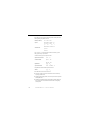
◆ Concert Technology is a set of C++, Java, and .NET class libraries offering an API that
includes modeling facilities to allow the programmer to embed CPLEX optimizers in
C++, Java, or .NET applications. Table 1. lists the files that contain the libraries.
Table 1 Concert Technology Libraries
Microsoft Windows
UNIX
C++
ilocplex.lib
concert.lib
libilocplex.a
libconcert.a
Java
cplex.jar
cplex.jar
.NET
ILOG.CPLEX.dll
ILOG.Concert.dll
The ILOG Concert Technology libraries make use of the Callable Library (described
next).
◆ The CPLEX Callable Library is a C library that allows the programmer to embed
ILOG CPLEX optimizers in applications written in C, Visual Basic, FORTRAN, or any
other language that can call C functions.The library is provided in files cplex100.lib
and cplex100.dll on Windows platforms, and in libcplex.a, libcplex.so, and
libcplex.sl on UNIX platforms.
In this manual, the phrase CPLEX Component Libraries is used to refer equally to any of
these libraries. While all of the libraries are callable, the term CPLEX Callable Library as
used here refers specifically to the C library.
Compatible Platforms
ILOG CPLEX is available on Windows, UNIX, and other platforms. The programming
interface works the same way and provides the same facilities on all platforms.
ILOG CPLEX 10.0
— GETTING STARTED
11
Installation Requirements
If you have not yet installed ILOG CPLEX on your platform, please consult Chapter 1,
Setting Up ILOG CPLEX. It contains instructions for installing ILOG CPLEX.
Optimizer Options
This manual explains how to use the LP algorithms that are part of ILOG CPLEX. The QP,
QCP, and MIP problem types are based on the LP concepts discussed here, and the
extensions to build and solve such problems are explained in the ILOG CPLEX User’s
Manual.
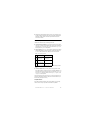
Default settings will result in a call to an optimizer that is appropriate to the class of problem
you are solving. However you may wish to choose a different optimizer for special purposes.
An LP or QP problem can be solved using any of the following CPLEX optimizers: Dual
Simplex, Primal Simplex, Barrier, and perhaps also the Network Optimizer (if the problem
contains an extractable network substructure). Pure network models are all solved by the
Network Optimizer. QCP models, including the special case of SOCP models, are all solved
by the Barrier optimizer. MIP models are all solved by the Mixed Integer Optimizer, which
in turn may invoke any of the LP or QP optimizers in the course of its computation. Table 2
summarizes these possible choices.
Table 2 Optimizers
LP
Network QP
Dual Optimizer
yes
yes
Primal Optimizer
yes
yes
Barrier Optimizer
yes
yes
MIP
yes
yes
Mixed Integer Optimizer
Network Optimizer
QCP
Note 1 yes
Note 1
Note 1: The problem must contain an extractable network substructure.
The choice of optimizer or other parameter settings may have a very large effect on the
solution speed of your particular class of problem. The ILOG CPLEX User's Manual
describes the optimizers, provides suggestions for maximizing performance, and notes the
features and algorithmic parameters unique to each optimizer.
Using the Parallel Optimizers
On a computer with multiple CPUs, the Barrier Optimizer and the MIP Optimizer are each
capable of running in parallel, that is, they can apply these additional CPUs to the task of
optimizing the model. The number of CPUs used by an optimizer is controlled by the user;
12
ILOG CPLEX 10.0
— GETTING STARTED
under default settings these optimizers run in serial (single CPU) mode. When solving small
models, such as those in this document, the effect of parallelism will generally be negligible.
On larger models, the effect is ordinarily beneficial to solution speed. See the section Using
Parallel Optimizers in the ILOG CPLEX User's Manual for information on using CPLEX on
a parallel computer.
Data Entry Options
CPLEX provides several options for entering your problem data. When using the Interactive
Optimizer, most users will enter problem data from formatted files. CPLEX supports the
industry-standard MPS (Mathematical Programming System) file format as well as CPLEX
LP format, a row-oriented format many users may find more natural. Interactive entry (using
CPLEX LP format) is also a possibility for small problems.
Data entry options are described briefly in this manual. File formats are documented in the
reference manual ILOG CPLEX File Formats.
Concert Technology and Callable Library users may read problem data from the same kinds
of files as in the Interactive Optimizer, or they may want to pass data directly into CPLEX to
gain efficiency. These options are discussed in a series of examples that begin with Building
and Solving a Small LP Model in C++, Building and Solving a Small LP Model in Java, and
Building and Solving a Small LP Model in C for the CPLEX Callable Library users.
What You Need to Know
In order to use ILOG CPLEX effectively, you need to be familiar with your operating
system, whether UNIX or Windows.
This manual assumes you already know how to create and manage files. In addition, if you
are building an application that uses the Component Libraries, this manual assumes that you
know how to compile, link, and execute programs written in a high-level language. The
Callable Library is written in the C programming language, while Concert Technology is
available for users of C++, Java, and the .NET framework. This manual also assumes that
you already know how to program in the appropriate language and that you will consult a
programming guide when you have questions in that area.
What’s in This Manual
Chapter 1, Setting Up ILOG CPLEX tells how to install CPLEX.
Chapter 2, Solving an LP with ILOG CPLEX shows you at a glance how to use the
Interactive Optimizer and each of the application programming interfaces (APIs): C++,
ILOG CPLEX 10.0
— GETTING STARTED
13
Java, .NET, and C. This overview is followed by more detailed tutorials about each
interface.
Chapter 3, Interactive Optimizer Tutorial, explains, step by step, how to use the Interactive
Optimizer: how to start it, how to enter problems and data, how to read and save files, how
to modify objective functions and constraints, and how to display solutions and analytical
information.
Chapter 4, Concert Technology Tutorial for C++ Users, describes the same activities using
the classes in the C++ implementation of the CPLEX Concert Technology Library.
Chapter 5, Concert Technology Tutorial for Java Users, describes the same activities using
the classes in the Java implementation of the CPLEX Concert Technology Library.
Chapter 6, Concert Technology Tutorial for .NET Users, describes the same activities using
.NET facilities.
Chapter 7, Callable Library Tutorial, describes the same activities using the routines in the
ILOG CPLEX Callable Library.
All tutorials use examples that are delivered with the standard distribution.
Notation in this Manual
This manual observes the following conventions in notation and names.
◆ Important ideas are emphasized the first time they appear.
◆ Text that is entered at the keyboard or displayed on the screen as well as commands and
their options available through the Interactive Optimizer appear in this typeface, for
example, set preprocessing aggregator n.
◆ Entries that you must fill in appear in this typeface; for example, write filename.
◆ The names of C routines and parameters in the ILOG CPLEX Callable Library begin
with CPX and appear in this typeface, for example, CPXcopyobjnames.
◆ The names of C++ classes in the CPLEX Concert Technology Library begin with Ilo
and appear in this typeface, for example, IloCplex.
◆ The names of Java classes begin with Ilo and appear in this typeface, for example,
IloCplex.
◆ The name of a class or method in .NET is written as concatenated words with the first
letter of each word in upper case, for example, IntVar or IntVar.VisitChildren.
Generally, accessors begin with the key word Get. Accessors for Boolean members
begin with Is. Modifiers begin with Set.
14
ILOG CPLEX 10.0
— GETTING STARTED
◆ Combinations of keys from the keyboard are hyphenated. For example, control-c
indicates that you should press the control key and the c key simultaneously. The symbol
<return> indicates end of line or end of data entry. On some keyboards, the key is
labeled enter or Enter.
Related Documentation
In addition to this introductory manual, the standard distribution of ILOG CPLEX comes
with the ILOG CPLEX User’s Manual and the ILOG CPLEX Reference Manual. All ILOG
documentation is available online in hypertext mark-up language (HTML). It is delivered
with the standard distribution of the product and accessible through conventional HTML
browsers.
◆ The ILOG CPLEX User’s Manual explains the relationship between the Interactive
Optimizer and the Component Libraries. It enlarges on aspects of linear programming
with ILOG CPLEX and shows you how to handle quadratic programming (QP)
problems, quadratically constrained programming (QCP) problems, second order cone
programming (SOCP) problems, and mixed integer programming (MIP) problems. It
tells you how to control ILOG CPLEX parameters, debug your applications, and
efficiently manage input and output. It also explains how to use parallel CPLEX
optimizers.
◆ The ILOG CPLEX Callable Library Reference Manual documents the Callable Library
routines and their arguments. This manual also includes additional documentation about
error codes, solution quality, and solution status. It is available online as HTML and
Microsoft compiled HTML help (.CHM).
◆ The ILOG CPLEX C++ API Reference Manual documents the C++ API of the Concert
Technology classes, methods, and functions. It is available online as HTML and
Microsoft compiled HTML help (.CHM).
◆ The ILOG CPLEX Java API Reference Manual supplies detailed definitions of the
Concert Technology interfaces and CPLEX Java classes. It is available online as HTML
and Microsoft compiled HTML help (.CHM).
◆ The ILOG CPLEX .NET Reference Manual documents the .NET API for CPLEX. It is
available online as HTML and Microsoft compiled HTML help (.CHM).
◆ The reference manual ILOG CPLEX Parameters contains a table of parameters that can
be modified by parameter routines. It is the definitive reference manual for the purpose
and allowable settings of CPLEX parameters.
◆ The reference manual ILOG CPLEX File Formats contains a list of file formats that
ILOG CPLEX supports as well as details about using them in your applications.
ILOG CPLEX 10.0
— GETTING STARTED
15
◆ The reference manual ILOG CPLEX Interactive Optimizer contains the commands of the
Interactive Optimizer, along with the command options and links to examples of their
use in the ILOG CPLEX User’s Manual.
As you work with ILOG CPLEX on a long-term basis, you should read the complete User’s
Manual to learn how to design models and implement solutions to your own problems.
Consult the reference manuals for authoritative documentation of the Component Libraries,
their application programming interfaces (APIs), and the Interactive Optimizer.
16
ILOG CPLEX 10.0
— GETTING STARTED
Part I
Setting Up
This part shows you how to set up ILOG CPLEX and how to check your installation. It
includes information for users of Microsoft and UNIX platforms.
C
H
A
P
T
E
R
1
Setting Up ILOG CPLEX
You install ILOG CPLEX in two steps: first, install the files from the distribution medium (a
CD or an FTP site) into a directory on your local file system; then activate your license.
At that point, all of the features of CPLEX become functional and are available to you. The
chapters that follow this one provide tutorials in the use of each of the Technologies that
ILOG CPLEX provides: the ILOG Concert Technology Tutorials for C++, Java, and .NET
users, and the Callable Library Tutorial for C and other languages.
This chapter provides guidelines for:
◆ Installing ILOG CPLEX on page 20
◆ Setting Up Licensing on page 22
◆ Using the Component Libraries on page 23
Important: Please read these instructions in their entirety before you begin the installation.
Remember that most ILOG CPLEX distributions will operate correctly only on the specific
platform and operating system for which they are designed. If you upgrade your operating
system, you may need to obtain a new ILOG CPLEX distribution.
ILOG CPLEX 10.0
— GETTING STARTED
19
Installing ILOG CPLEX
The steps to install ILOG CPLEX involve identifying the correct distribution file for your
particular platform, and then executing a command that uses that distribution file. The
identification step is explained in the booklet that comes with the CD-ROM, or is provided
with the FTP instructions for download. After the correct distribution file is at hand, the
installation proceeds as follows.
Installation on UNIX
On UNIX systems ILOG CPLEX 10.0 is installed in a subdirectory named cplex100,
under the current working directory where you perform the installation.
Use the cd command to move to the top level directory into which you want to install the
cplex subdirectory. Then type this command:
gzip -dc < path/cplex.tgz | tar xf -
where path is the full path name pointing to the location of the ILOG CPLEX distribution
file (either on the CD-ROM or on a disk where you performed the FTP download). On
UNIX systems, both ILOG CPLEX and ILOG Concert Technology are installed when you
execute that command.
Installation on Windows
Before you install ILOG CPLEX, you need to identify the correct distribution file for your
platform. There are instructions on how to identify your distribution in the booklet that
comes with the CD-ROM or with the FTP instructions for download. This booklet also tells
how to start the ILOG CPLEX installation on your platform.
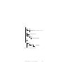
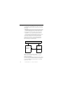
Directory Structure
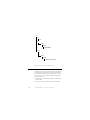
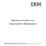
After completing the installation, you will have a directory structure like the one in
Figure 1.1 and Figure 1.2.
Be sure to read the readme.html carefully for the most recent information about the
version of ILOG CPLEX you have installed.
20
ILOG CPLEX 10.0
— GETTING STARTED
Figure 1.1
cplex
bin
platform
EXECUTABLE FILES
(Interactive Optimizer, .dll and .so files)
examples
data
src
tutorials (available only for .NET)
platform
lib format
Makefile or MSVC++ project files
include
ilcplex
lib
platform
lib format
CPLEX LIBRARY
Java LIBRARY cplex.jar
Figure 1.1 Structure of the ILOG CPLEX installation directory
ILOG CPLEX 10.0
— GETTING STARTED
21
Figure 1.2
concert
include
ilconcert
lib
platform
lib format
CONCERT LIBRARY
examples
data
src
platform
lib format
Makefile or MSVC++ project files
Figure 1.2 Structure of the Concert Technology Installation Directory
Setting Up Licensing
ILOG CPLEX 10.0 runs under the control of the ILOG License Manager (ILM). Before you
can run ILOG CPLEX, or any application that calls it, you must have established a valid
license that ILM can read. Licensing instructions are provided in the ILOG License Manager
User’s Guide & Reference, which is included with the standard ILOG CPLEX product
distribution. The basic steps are:
1. Install ILM. Normally you obtain ILM distribution media from the same place that you
obtain ILOG CPLEX.
2. Run the ihostid program, which is found in the directory where you install ILM.
22
ILOG CPLEX 10.0
— GETTING STARTED
3. Communicate the output of step 2 to your local ILOG sales administration department.
They will send you a license key in return. One way to communicate the results of step 2
to your local ILOG sales administration department is through the web page serving your
region.
Europe and Africa: https://support.ilog.fr/license/index.cfm
Americas: https://support.ilog.com/license/index.cfm
Asia: https://support.ilog.com.sg/license/index.cfm
4. Create a file on your system to hold this license key, and set the environment variable
ILOG_LICENSE_FILE so that ILOG CPLEX will know where to find the license key.
(The environment variable need not be used if you install the license key in a platformdependent default file location.)
Using the Component Libraries
After you have completed the installation and licensing steps, you can verify that everything
is working by running one or more of the examples that are provided with the standard
distribution.
Verifying Installation on UNIX
On a UNIX system, go to the subdirectory examples/machine/libformat that matches
your particular platform, and in it you will find a file named Makefile. Execute one of the
examples, for instance lpex1.c, by doing
make lpex1
lpex1 -r
# this example takes one argument, either -r, -c, or -n
If your interest is in running one of the C++ examples, try
make ilolpex1
ilolpex1 -r # this is the same as lpex1 and takes the same arguments.
If your interest is in running one of the Java examples, try
make LPex1.class
java -Djava.library.path=../../../bin/<platform>: \
-classpath ../../../lib/cplex.jar: LPex1 -r
Any of these examples should return an optimal objective function value of 202.5.
ILOG CPLEX 10.0
— GETTING STARTED
23
Verifying Installation on Windows
On a Windows machine, you can follow a similar process using the facilities of your
compiler interface to compile and then run any of the examples. A project file for each
example is provided, in a format for Microsoft Visual Studio 6 and Visual Studio .NET.
In Case of Errors
If an error occurs during the make or compile step, then check that you are able to access the
compiler and the necessary linker/loader files and system libraries. If an error occurs on the
next step, when executing the program created by make, then the nature of the error message
will guide your actions. If the problem is in licensing, consult the ILOG License Manager
User's Guide and Reference for further guidance. For Windows users, if the program has
trouble locating cplex100.dll or ILOG.CPLEX.dll, make sure the DLL is stored either
in the current directory or in a directory listed in your PATH environment variable.
The UNIX Makefile, or Windows project file, contains useful information regarding
recommended compiler flags and other settings for compilation and linking.
Compiling and Linking Your Own Applications
The source files for the examples and the makefiles provide guidance for how your own
application can call ILOG CPLEX. The following chapters give more specific information
on the necessary header files for compilation, and how to link ILOG CPLEX and Concert
Technology libraries into your application.
◆ Chapter 4, Concert Technology Tutorial for C++ Users contains information and
platform-specific instructions for compiling and linking the Concert Technology Library,
for C++ users.
◆ Chapter 5, Concert Technology Tutorial for Java Users contains information and
platform-specific instructions for compiling and linking the Concert Technology Library,
for Java users.
◆ Chapter 6, Concert Technology Tutorial for .NET Users offers an example of a C#.NET
application.
◆ Chapter 7, Callable Library Tutorial contains information and platform-specific
instructions for compiling and linking the Callable Library.
24
ILOG CPLEX 10.0
— GETTING STARTED
Part II
Tutorials
This part provides tutorials to introduce you to each of the components of ILOG CPLEX.
◆ Interactive Optimizer Tutorial on page 35
◆ Concert Technology Tutorial for C++ Users on page 69
◆ Concert Technology Tutorial for Java Users on page 87
◆ Concert Technology Tutorial for .NET Users on page 99
◆ Callable Library Tutorial on page 111
C
H
A
P
T
E
R
2
Solving an LP with ILOG CPLEX
To help you learn which CPLEX component best meets your needs, this chapter briefly
demonstrates how to create and solve an LP model. It shows you at a glance the Interactive
Optimizer and the application programming interfaces (APIs) to CPLEX. Full details of
writing a practical program are in the chapters containing the tutorials.
◆ Problem Statement on page 28
◆ Using the Interactive Optimizer on page 29
◆ Using Concert Technology in C++ on page 30
◆ Using Concert Technology in Java on page 31
◆ Using Concert Technology in .NET on page 32
◆ Using the Callable Library on page 33
ILOG CPLEX 10.0
— GETTING STARTED
27
Problem Statement
The problem to be solved is:
Maximize
28
x1 + 2x2 + 3x3
subject to
–x1 + x2 + x3 ≤ 20
x1 – 3x2 + x3 ≤ 30
with these bounds
0 ≤ x1 ≤ 40
0 ≤ x2 ≤ +∞
0 ≤ x3 ≤ +∞
ILOG CPLEX 10.0
— GETTING STARTED
Using the Interactive Optimizer
The following sample is screen output from a CPLEX Interactive Optimizer session where
the model of an example is entered and solved. CPLEX> indicates the CPLEX prompt, and
text following this prompt is user input.
Welcome to CPLEX Interactive Optimizer 10.0.0
with Simplex, Mixed Integer & Barrier Optimizers
Copyright (c) ILOG 1997-2006
CPLEX is a registered trademark of ILOG
Type 'help' for a list of available commands.
Type 'help' followed by a command name for more
information on commands.
CPLEX> enter example
Enter new problem ['end' on a separate line terminates]:
maximize x1 + 2 x2 + 3 x3
subject to -x1 + x2 + x3 <= 20
x1 - 3 x2 + x3 <=30
bounds
0 <= x1 <= 40
0 <= x2
0 <= x3
end
CPLEX> optimize
Tried aggregator 1 time.
No LP presolve or aggregator reductions.
Presolve time =
0.00 sec.
Iteration log . . .
Iteration:
1
Dual infeasibility =
Iteration:
2
Dual objective
=
0.000000
202.500000
Dual simplex - Optimal: Objective =
2.0250000000e+002
Solution time =
0.01 sec. Iterations = 2 (1)
CPLEX> display solution variables x1-x3
Variable Name
Solution Value
x1
40.000000
x2
17.500000
x3
42.500000
CPLEX> quit
ILOG CPLEX 10.0
— GETTING STARTED
29
Using Concert Technology in C++
Here is a C++ application using ILOG CPLEX in Concert Technology to solve the example.
An expanded form of this example is discussed in detail in Concert Technology Tutorial for
C++ Users on page 69.
#include <ilcplex/ilocplex.h>
ILOSTLBEGIN
int
main (int argc, char **argv)
{
IloEnv env;
try {
IloModel model(env);
IloNumVarArray vars(env);
vars.add(IloNumVar(env, 0.0, 40.0));
vars.add(IloNumVar(env));
vars.add(IloNumVar(env));
model.add(IloMaximize(env, vars[0] + 2 * vars[1] + 3 * vars[2]));
model.add( - vars[0] +
vars[1] + vars[2] <= 20);
model.add(
vars[0] - 3 * vars[1] + vars[2] <= 30);
IloCplex cplex(model);
if ( !cplex.solve() ) {
env.error() << "Failed to optimize LP." << endl;
throw(-1);
}
IloNumArray vals(env);
env.out() << "Solution status = " << cplex.getStatus() << endl;
env.out() << "Solution value = " << cplex.getObjValue() << endl;
cplex.getValues(vals, vars);
env.out() << "Values = " << vals << endl;
}
catch (IloException& e) {
cerr << "Concert exception caught: " << e << endl;
}
catch (...) {
cerr << "Unknown exception caught" << endl;
}
env.end();
}
30
return 0;
// END main
ILOG CPLEX 10.0
— GETTING STARTED
Using Concert Technology in Java
Here is a Java application using ILOG CPLEX with Concert Technology to solve the
example. An expanded form of this example is discussed in detail in Chapter 5, Concert
Technology Tutorial for Java Users.
import ilog.concert.*;
import ilog.cplex.*;
public class Example {
public static void main(String[] args) {
try {
IloCplex cplex = new IloCplex();
double[]
lb = {0.0, 0.0, 0.0};
double[]
ub = {40.0, Double.MAX_VALUE, Double.MAX_VALUE};
IloNumVar[] x = cplex.numVarArray(3, lb, ub);
double[] objvals = {1.0, 2.0, 3.0};
cplex.addMaximize(cplex.scalProd(x, objvals));
cplex.addLe(cplex.sum(cplex.prod(-1.0,
cplex.prod( 1.0,
cplex.prod( 1.0,
cplex.addLe(cplex.sum(cplex.prod( 1.0,
cplex.prod(-3.0,
cplex.prod( 1.0,
x[0]),
x[1]),
x[2])), 20.0);
x[0]),
x[1]),
x[2])), 30.0);
if ( cplex.solve() ) {
cplex.output().println("Solution status = " + cplex.getStatus());
cplex.output().println("Solution value = " + cplex.getObjValue());
double[] val = cplex.getValues(x);
int ncols = cplex.getNcols();
for (int j = 0; j < ncols; ++j)
cplex.output().println("Column: " + j + " Value = " + val[j]);
}
cplex.end();
}
catch (IloException e) {
System.err.println("Concert exception '" + e + "' caught");
}
}
}
ILOG CPLEX 10.0
— GETTING STARTED
31
Using Concert Technology in .NET
There is an interactive tutorial, based on that same example, for .NET users of
ILOG CPLEX in Chapter 6, Concert Technology Tutorial for .NET Users.
32
ILOG CPLEX 10.0
— GETTING STARTED
Using the Callable Library
Here is a C application using the CPLEX Callable Library to solve the example. An
expanded form of this example is discussed in detail in Chapter 7, Callable Library Tutorial.
#include <ilcplex/cplex.h>
#include <stdlib.h>
#include <string.h>
#define NUMROWS
#define NUMCOLS
#define NUMNZ
2
3
6
int
main (int argc, char **argv)
{
int
status = 0;
CPXENVptr env = NULL;
CPXLPptr lp = NULL;
double
double
double
double
int
int
double
double
char
obj[NUMCOLS];
lb[NUMCOLS];
ub[NUMCOLS];
x[NUMCOLS];
rmatbeg[NUMROWS];
rmatind[NUMNZ];
rmatval[NUMNZ];
rhs[NUMROWS];
sense[NUMROWS];
int
double
solstat;
objval;
env = CPXopenCPLEX (&status);
if ( env == NULL ) {
char errmsg[1024];
fprintf (stderr, "Could not open CPLEX environment.\n");
CPXgeterrorstring (env, status, errmsg);
fprintf (stderr, "%s", errmsg);
goto TERMINATE;
}
lp = CPXcreateprob (env, &status, "lpex1");
if ( lp == NULL ) {
fprintf (stderr, "Failed to create LP.\n");
goto TERMINATE;
}
CPXchgobjsen (env, lp, CPX_MAX);
obj[0] = 1.0;
lb[0] = 0.0;
ub[0] = 40.0;
obj[1] = 2.0;
lb[1] = 0.0;
ub[1] = CPX_INFBOUND;
obj[2] = 3.0;
lb[2] = 0.0;
ub[2] = CPX_INFBOUND;
status = CPXnewcols (env, lp, NUMCOLS, obj, lb, ub, NULL, NULL);
if ( status ) {
ILOG CPLEX 10.0
— GETTING STARTED
33
fprintf (stderr, "Failed to populate problem.\n");
goto TERMINATE;
}
rmatbeg[0] = 0;
rmatind[0] = 0;
rmatval[0] = -1.0;
rmatbeg[1] = 3;
rmatind[3] = 0;
rmatval[3] = 1.0;
rmatind[1] = 1;
rmatval[1] = 1.0;
rmatind[2] = 2; sense[0] = 'L';
rmatval[2] = 1.0; rhs[0] = 20.0;
rmatind[4] = 1;
rmatind[5] = 2;
rmatval[4] = -3.0; rmatval[5] = 1.0;
sense[1] = 'L';
rhs[1]
= 30.0;
status = CPXaddrows (env, lp, 0, NUMROWS, NUMNZ, rhs, sense, rmatbeg,
rmatind, rmatval, NULL, NULL);
if ( status ) {
fprintf (stderr, "Failed to populate problem.\n");
goto TERMINATE;
}
status = CPXlpopt (env, lp);
if ( status ) {
fprintf (stderr, "Failed to optimize LP.\n");
goto TERMINATE;
}
status = CPXsolution (env, lp, &solstat, &objval, x, NULL, NULL, NULL);
if ( status ) {
fprintf (stderr, "Failed to obtain solution.\n");
goto TERMINATE;
}
printf ("\nSolution status = %d\n", solstat);
printf ("Solution value = %f\n", objval);
printf ("Solution
= [%f, %f, %f]\n\n", x[0], x[1], x[2]);
TERMINATE:
if ( lp != NULL ) {
status = CPXfreeprob (env, &lp);
if ( status ) {
fprintf (stderr, "CPXfreeprob failed, error code %d.\n", status);
}
}
if ( env != NULL ) {
status = CPXcloseCPLEX (&env);
if ( status ) {
char errmsg[1024];
fprintf (stderr, "Could not close CPLEX environment.\n");
CPXgeterrorstring (env, status, errmsg);
fprintf (stderr, "%s", errmsg);
}
}
return (status);
}
34
/* END main */
ILOG CPLEX 10.0
— GETTING STARTED
C
H
A
P
T
E
R
3
Interactive Optimizer Tutorial
This step-by-step tutorial introduces the major features of the ILOG CPLEX Interactive
Optimizer. In this chapter, you will learn about:
◆ Starting ILOG CPLEX on page 36;
◆ Using Help on page 36;
◆ Entering a Problem on page 38;
◆ Displaying a Problem on page 42;
◆ Solving a Problem on page 48;
◆ Performing Sensitivity Analysis on page 51;
◆ Writing Problem and Solution Files on page 53;
◆ Reading Problem Files on page 55;
◆ Setting ILOG CPLEX Parameters on page 58;
◆ Adding Constraints and Bounds on page 60;
◆ Changing a Problem on page 61;
◆ Executing Operating System Commands on page 66;
◆ Quitting ILOG CPLEX on page 66.
ILOG CPLEX 10.0
— GETTING STARTED
35
Starting ILOG CPLEX
To start the ILOG CPLEX Interactive Optimizer, at your operating system prompt type the
command:
cplex
A message similar to the following one appears on the screen:
Welcome to CPLEX Interactive Optimizer 10.0.0
with Simplex, Mixed Integer & Barrier Optimizers
Copyright (c) ILOG 1997-2006
CPLEX is a registered trademark of ILOG
Type help for a list of available commands.
Type help followed by a command name for more
information on commands.
CPLEX>
The last line, CPLEX>, is the prompt, indicating that the product is running and is ready to
accept one of the available ILOG CPLEX commands. Use the help command to see a list of
these commands.
Using Help
ILOG CPLEX accepts commands in several different formats. You can type either the full
command name, or any shortened form that uniquely identifies that name. For example,
enter help after the CPLEX> prompt, as shown:
CPLEX> help
You will see a list of the ILOG CPLEX commands on the screen.
Since all commands start with a unique letter, you could also enter just the single letter h.
CPLEX> h
ILOG CPLEX does not distinguish between upper- and lower-case letters, so you could
enter h, H, help, or HELP. All of these variations invoke the help command. The same rules
apply to all ILOG CPLEX commands. You need only type enough letters of the command to
distinguish it from all other commands, and it does not matter whether you type upper- or
lower-case letters. This manual uses lower-case letters.
36
ILOG CPLEX 10.0
— GETTING STARTED
After you type the help command, a list of available commands with their descriptions
appears on the screen, like this:
add
baropt
change
conflict
display
enter
feasopt
help
mipopt
netopt
optimize
primopt
quit
read
set
tranopt
write
xecute
add constraints to the problem
solve using barrier algorithm
change the problem
refine a conflict for an infeasible problem
display problem, solution, or parameter settings
enter a new problem
find relaxation to infeasible linear problem
provide information on CPLEX commands
solve a mixed integer program
solve the problem using network method
solve the problem
solve using the primal method
leave CPLEX
read problem or advanced start information from a file
set parameters
solve using the dual method
write problem or solution information to a file
execute a command from the operating system
Enter enough characters to uniquely identify commands & options.
Commands can be entered partially (CPLEX will prompt you for
further information) or as a whole.
To find out more about a specific command, type help followed by the name of that
command. For example, to learn more about the primopt command type:
help primopt
Typing the full name is unnecessary. Alternatively, you can try:
h p
The following message appears to tell you more about the use and syntax of the primopt
command:
The PRIMOPT command solves the current problem using
a primal simplex method or crosses over to a basic solution
if a barrier solution exists.
Syntax:
PRIMOPT
A problem must exist in memory (from using either the
ENTER or READ command) in order to use the PRIMOPT
command.
Sensitivity information (dual price and reduced-cost
information) as well as other detailed information about
the solution can be viewed using the DISPLAY command,
after a solution is generated.
Summary
The syntax for the help command is:
ILOG CPLEX 10.0
— GETTING STARTED
37
help command name
Entering a Problem
Most users with larger problems enter problems by reading data from formatted files. That
practice is explained in Reading Problem Files on page 55. For now, you will enter a smaller
problem from the keyboard by using the enter command. The process is outlined
step-by-step in these topics:
◆ Entering the Example Problem on page 38;
◆ Using the LP Format on page 39;
◆ Entering Data on page 41.
Entering the Example Problem
As an example, this manual uses the following problem:
Maximize
x1 + 2x2 + 3x3
subject to
–x1 + x2 + x3 ≤ 20
x1 – 3x2 + x3 ≤ 30
with these bounds
0 ≤ x1 ≤ 40
0 ≤ x2 ≤ +∞
0 ≤ x3 ≤ +∞
This problem has three variables (x1, x2, and x3) and two less-than-or-equal-to constraints.
The enter command is used to enter a new problem from the keyboard. The procedure is
almost as simple as typing the problem on a page. At the CPLEX> prompt type:
enter
A prompt appears on the screen asking you to give a name to the problem that you are about
to enter.
Naming a Problem
The problem name may be anything that is allowed as a file name in your operating system.
If you decide that you do not want to enter a new problem, just press the <return> key
without typing anything. The CPLEX> prompt will reappear without causing any action. The
same can be done at any CPLEX> prompt. If you do not want to complete the command,
simply press the <return> key. For now, type in the name example at the prompt.
Enter name for problem: example
38
ILOG CPLEX 10.0
— GETTING STARTED
The following message appears:
Enter new problem ['end' on a separate line terminates]:
and the cursor is positioned on a blank line below it where you can enter the new problem.
You can also type the problem name directly after the enter command and avoid the
intermediate prompt.
Summary
The syntax for entering a problem is:
enter problem name
Using the LP Format
Entering a new problem is basically like typing it on a page, but there are a few rules to
remember. These rules conform to the ILOG CPLEX LP file format and are documented in
the reference manual ILOG CPLEX File Formats. LP format appears throughout this
tutorial.
The problem should be entered in the following order:
1. Objective Function
2. Constraints
3. Bounds
Objective Function
Before entering the objective function, you must state whether the problem is a
minimization or maximization. For this example, you type:
maximize
x1 + 2x2 + 3x3
You may type minimize or maximize on the same line as the objective function, but you
must separate them by at least one space.
Variable Names
In the example, the variables are named simply x1, x2, x3, but you can give your variables
more meaningful names such as cars or gallons. The only limitations on variable names
in LP format are that the names must be no more than 255 characters long and use only the
alphanumeric characters (a-z, A-Z, 0-9) and certain symbols: ! " # $ % & ( ) , . ; ? @ _ ‘ ’ { }
~. Any line with more than 510 characters is truncated.
A variable name cannot begin with a number or a period, and there is one character
combination that cannot be used: the letter e or E alone or followed by a number or another
e, since this notation is reserved for exponents. Thus, a variable cannot be named e24 nor
ILOG CPLEX 10.0
— GETTING STARTED
39
e9cats nor eels nor any other name with this pattern. This restriction applies only to
problems entered in LP format.
Constraints
After you have entered the objective function, you can move on to the constraints. However,
before you start entering the constraints, you must indicate that the subsequent lines are
constraints by typing:
subject to
or
st
These terms can be placed alone on a line or on the same line as the first constraint if
separated by at least one space. Now you can type in the constraints in the following way:
st
-x1 + x2 + x3 <= 20
x1 - 3x2 + x3 <= 30
Constraint Names
In this simple example, it is easy to keep track of the small number of constraints, but for
many problems, it may be advantageous to name constraints so that they are easier to
identify. You can do so in ILOG CPLEX by typing a constraint name and a colon before the
actual constraint. If you do not give the constraints explicit names, ILOG CPLEX will give
them the default names c1, c2, . . . , cn. In the example, if you want to call the
constraints time and labor, for example, enter the constraints like this:
st
time: -x1 + x2 + x3 <= 20
labor: x1 - 3x2 + x3 <= 30
Constraint names are subject to the same guidelines as variable names. They must have no
more than 255 characters, consist of only allowed characters, and not begin with a number, a
period, or the letter e followed by a positive or negative number or another e.
Objective Function Names
The objective function can be named in the same manner as constraints. The default name
for the objective function is obj. ILOG CPLEX assigns this name if no other is entered.
Bounds
Finally, you must enter the lower and upper bounds on the variables. If no bounds are
specified, ILOG CPLEX will automatically set the lower bound to 0 and the upper bound to
+∞. You must explicitly enter bounds only when the bounds differ from the default values.
In our example, the lower bound on x1 is 0, which is the same as the default. The upper
bound 40, however, is not the default, so you must enter it explicitly. You must type bounds
on a separate line before you enter the bound information:
40
ILOG CPLEX 10.0
— GETTING STARTED
bounds
x1 <= 40
Since the bounds on x2 and x3 are the same as the default bounds, there is no need to enter
them. You have finished entering the problem, so to indicate that the problem is complete,
type:
end
on the last line.
The CPLEX> prompt returns, indicating that you can again enter a ILOG CPLEX command.
Summary
Entering a problem in ILOG CPLEX is straightforward, provided that you observe a few
simple rules:
◆ The terms maximize or minimize must precede the objective function; the term
subject to must precede the constraints section; both must be separated from the
beginning of each section by at least one space.
◆ The word bounds must be alone on a line preceding the bounds section.
◆ On the final line of the problem, end must appear.
Entering Data
You can use the <return> key to split long constraints, and ILOG CPLEX still interprets
the multiple lines as a single constraint. When you split a constraint in this way, do not press
<return> in the middle of a variable name or coefficient. The following is acceptable:
time: -x1 + x2 + <return>
x3 <= 20 <return>
labor: x1 - 3x2 + x3 <= 30
<return>
The entry below, however, is incorrect since the <return> key splits a variable name.
time: -x1 + x2 + x <return>
3 <= 20 <return>
labor: x1 - 3x2 + x3 <= 30
<return>
If you type a line that ILOG CPLEX cannot interpret, a message indicating the problem will
appear, and the entire constraint or objective function will be ignored. You must then
re-enter the constraint or objective function.
The final thing to remember when you are entering a problem is that after you have pressed
<return>, you can no longer directly edit the characters that precede the <return>. As
long as you have not pressed the <return> key, you can use the <backspace> key to go
back and change what you typed on that line. After <return> has been pressed, the change
command must be used to modify the problem. The change command is documented in
Changing a Problem on page 61.
ILOG CPLEX 10.0
— GETTING STARTED
41
Displaying a Problem
Now that you have entered a problem using ILOG CPLEX, you must verify that the problem
was entered correctly. To do so, use the display command. At the CPLEX> prompt type:
display
A list of the items that can be displayed then appears. Some of the options display parts of
the problem description, while others display parts of the problem solution. Options about
the problem solution are not available until after the problem has been solved. The list looks
like this:
Display Options:
conflict
problem
sensitivity
settings
solution
display
display
display
display
display
conflict that demonstrates model infeasibility
problem characteristics
sensitivity analysis
parameter settings
existing solution
Display what:
If you type problem in reply to that prompt, that option will list a set of problem
characteristics, like this:
Display Problem Options:
all
binaries
bounds
constraints
generals
histogram
integers
names
qpvariables
semi-continuous
sos
stats
variable
display
display
display
display
display
display
display
display
display
display
display
display
display
entire problem
binary variables
a set of bounds
a set of constraints or node supply/demand values
general integer variables
a histogram of row or column counts
integer variables
names of variables or constraints
quadratic variables
semi-continuous and semi-integer variables
special ordered sets
problem statistics
a column of the constraint matrix
Display which problem characteristic:
Enter the option all to display the entire problem.
Maximize
obj: x1 + 2 x2 + 3 x3
Subject To
c1: - x1 +
x2 +
x3 <= 20
c2: x1 - 3 x2 +
x3 <= 30
Bounds
0 <= x1 <= 40
All other variables are >= 0.
42
ILOG CPLEX 10.0
— GETTING STARTED
The default names obj, c1, c2, are provided by ILOG CPLEX.
If that is what you want, you are ready to solve the problem. If there is a mistake, you must
use the change command to modify the problem. The change command is documented in
Changing a Problem on page 61.
Summary
Display problem characteristics by entering the command:
display problem
Displaying Problem Statistics
When the problem is as small as our example, it is easy to display it on the screen; however,
many real problems are far too large to display. For these problems, the stats option of the
display problem command is helpful. When you select stats, information about the
attributes of the problem appears, but not the entire problem itself. These attributes include:
◆ the number and type of constraints
◆ variables
◆ nonzero constraint coefficients
Try this feature by typing:
display problem stats
For our example, the following information appears:
Problem name: example
Variables
:
Objective nonzeros
:
Linear constraints
:
Nonzeros
:
RHS nonzeros
:
3
3
2
6
2
[Nneg: 2,
Box: 1]
[Less: 2]
This information tells us that in the example there are two constraints, three variables, and
six nonzero constraint coefficients. The two constraints are both of the type
less-than-or-equal-to. Two of the three variables have the default nonnegativity bounds
(0 ≤ x ≤ +∞) and one is restricted to a certain range (a box variable). In addition to a
constraint matrix nonzero count, there is a count of nonzero coefficients in the objective
function and on the righthand side. Such statistics can help to identify errors in a problem
without displaying it in its entirety.
You can see more information about the values of the input data in your problem if you set
the datacheck parameter before you type the comman display problem stats.
(Parameters are explained Setting ILOG CPLEX Parameters on page 58 later in this
tutorial.) To set the datacheck parameter, type the following for now:
set read datacheck yes
ILOG CPLEX 10.0
— GETTING STARTED
43
With this setting, the command display problem stats shows this additional
information:
Variables
Objective nonzeros
Linear constraints
Nonzeros
RHS nonzeros
:
:
:
:
:
Min LB: 0.000000
Min
: 1.000000
Max UB: 40.00000
Max
: 3.000000
Min
Min
Max
Max
: 1.000000
: 20.00000
: 3.000000
: 30.00000
Another way to avoid displaying an entire problem is to display a specific part of it by using
one of the following three options of the display problem command:
◆ names, documented in Displaying Variable or Constraint Names on page 44, can be
used to display a specified set of variable or constraint names;
◆ constraints, documented in Displaying Constraints on page 46, can be used to
display a specified set of constraints;
◆ bounds, documented in Displaying Bounds on page 46, can be used to display a
specified set of bounds.
Specifying Item Ranges
For some options of the display command, you must specify the item or range of items
you want to see. Whenever input defining a range of items is required, ILOG CPLEX
expects two indices separated by a hyphen (the range character -). The indices can be names
or matrix index numbers. You simply enter the starting name (or index number), a hyphen
( – ), and finally the ending name (or index number). ILOG CPLEX automatically sets the
default upper and lower limits defining any range to be the highest and lowest possible
values. Therefore, you have the option of leaving out either the upper or lower name (or
index number) on either side of the hyphen. To see every possible item, you would simply
enter –.
Another way to specify a range of items is to use a wildcard. ILOG CPLEX accepts these
wildcards in place of the hyphen to specify a range of items:
◆ question mark (?) for a single character;
◆ asterisk (*) for zero or more characters.
For example, to specify all items, you could enter * (instead of -) if you want.
The sequence of characters c1? matches the name of every constraint in the range from c10
to c19, for example.
Displaying Variable or Constraint Names
You can display a variable name by using the display command with the options
problem names variables. If you do not enter the word variables, ILOG CPLEX
prompts you to specify whether you wish to see a constraint or variable name.
44
ILOG CPLEX 10.0
— GETTING STARTED
Type the following command:
display problem names variables
In response, ILOG CPLEX prompts you to specify a set of variable names to be displayed,
like this:
Display which variable name(s):
Specify these variables by entering the names of the variables or the numbers corresponding
to the columns of those variables. A single number can be used or a range such as 1-2. All
of the names can be displayed at after if you type a hyphen (the character - ). Try this by
entering a hyphen at the prompt and pressing the <return> key.
Display which variable name(s): -
You could also use a wildcard to display variable names, like this:
Display which variable name(s): *
In the example, there are three variables with default names. ILOG CPLEX displays these
three names:
x1
x2
x3
If you want to see only the second and third names, you could either enter the range as 2-3
or specify everything following the second variable with 2-. Try this technique:
display problem names variables
Display which variable name(s): 2x2 x3
If you enter a number without a hyphen, you will see a single variable name:
display problem names variables
Display which variable name(s): 2
x2
Summary
◆ You can use a wildcard in the display command to specify a range of items.
◆ You can display variable names by entering the command:
display problem names variables
◆ You can display constraint names by entering the command:
display problem names constraints
Ordering Variables
In the example problem there is a direct correlation between the variable names and their
numbers (x1 is variable 1, x2 is variable 2, etc.); that is not always the case. The internal
ILOG CPLEX 10.0
— GETTING STARTED
45
ordering of the variables is based on their order of occurrence when the problem is entered.
For example, if x2 had not appeared in the objective function, then the order of the variables
would be x1, x3, x2.
You can see the internal ordering by using the hyphen when you specify the range for the
variables option. The variables are displayed in the order corresponding to their internal
ordering.
All of the options of the display command can be entered directly after the word display
to eliminate intermediate steps. The following command is correct, for example:
display problem names variables 2-3
Displaying Constraints
To view a single constraint within the matrix, use the command and the constraint number.
For example, type the following:
display problem constraints 2
The second constraint appears:
c2: x1 - 3 x2 + x3 <= 30
You can also use a wildcard to display a range of constraints, like this:
display problem constraints *
Displaying the Objective Function
When you want to display only the objective function, you must enter its name (obj by
default) or an index number of 0.
display problem constraints
Display which constraint name(s): 0
Maximize
obj: x1 + 2 x2 + 3 x3
Displaying Bounds
To see only the bounds for the problem, type the following command (don’t forget the
hyphen or wildcard):
display problem bounds -
or, try a wildcard, like this:
display problem bounds *
The result is:
0 <= x1 <= 40
46
ILOG CPLEX 10.0
— GETTING STARTED
All other variables are >= 0.
Summary
The general syntax of the display command is:
display option [option2] identifier - [identifier2]
Displaying a Histogram of NonZero Counts
For large models, it can sometimes be helpful to see summaries of nonzero counts of the
columns or rows of the constraint matrix. This kind of display is known as a histogram.
There are two commands for displaying histograms: one for columns, one for rows.
display problem histogram c
display problem histogram r
For the small example in this tutorial, the column histogram looks like this:
Column counts (excluding fixed variables):
Nonzero Count:
Number of Columns:
2
3
It tells you that there are three columns each having two nonzeroes, and no other columns.
Similarly, the row histogram of the same small problem looks like this:
Row counts (excluding fixed variables):
Nonzero Count:
Number of Rows:
3
2
It tells you that there are two rows with three nonzeroes in each of them.
Of course, in a more complex model, there would usually be a wider variety of nonzero
counts than those histograms show. Here is an example in which there are sixteen columns
where only one row is non zero, 756 columns where two rows are non zero, and so forth.
Column counts (excluding fixed variables):
Nonzero Count:
1
2
3
4
Number of Columns:
16
756 1054
547
5
267
6
113
15
2
16
1
If there has been an error during entry of the problem, perhaps a constraint coefficient
having been omitted by mistake, for example, summaries like these, of a model where the
structure of the constraint matrix is known, may help you find the source of the error.
ILOG CPLEX 10.0
— GETTING STARTED
47
Solving a Problem
The problem is now correctly entered, and ILOG CPLEX can be used to solve it. This
example continues with the following topics:
◆ Solving the Example Problem on page 48;
◆ Solution Options on page 49;
◆ Displaying Post-Solution Information on page 50.
Solving the Example Problem
The optimize command tells ILOG CPLEX to solve the LP problem. ILOG CPLEX uses
the dual simplex optimizer, unless another method has been specified by setting the
LPMETHOD parameter (explained more fully in the ILOG CPLEX User’s Manual).
Entering the Optimize Command
At the CPLEX> prompt, type the command:
optimize
Preprocessing
First, ILOG CPLEX tries to simplify or reduce the problem using its presolver and
aggregator. If any reductions are made, a message will appear. However, in our small
example, no reductions are possible.
Monitoring the Iteration Log
Next, an iteration log appears on the screen. ILOG CPLEX reports its progress as it solves
the problem. The solution process involves two stages:
◆ during Phase I, ILOG CPLEX searches for a feasible solution
◆ in Phase II, ILOG CPLEX searches for the optimal feasible solution.
The iteration log periodically displays the current iteration number and either the current
scaled infeasibility during Phase I, or the objective function value during Phase II. After the
optimal solution has been found, the objective function value, solution time, and iteration
count (total, with Phase I in parentheses) are displayed. This information can be useful for
monitoring the rate of progress.
The iteration log display can be modified by the set simplex display command to
display differing amounts of data while the problem is being solved.
Reporting the Solution
After it finds the optimal solution, ILOG CPLEX reports:
◆ the objective function value
48
ILOG CPLEX 10.0
— GETTING STARTED
◆ the problem solution time in seconds
◆ the total iteration count
◆ the Phase I iteration count (in parentheses)
Optimizing our example problem produces a report like the following one (although the
solution times vary with each computer):
Tried aggregator 1 time.
No presolve or aggregator reductions.
Presolve Time = 0.00 sec.
Iteration Log . . .
Iteration:
1 Dual infeasibility =
Iteration:
2 Dual objective
=
0.000000
202.500000
Dual simplex - Optimal: Objective =
2.0250000000e+02
Solution Time =
0.00 sec. Iterations = 2 (1)
CPLEX>
In our example, ILOG CPLEX finds an optimal solution with an objective value of 202.5 in
two iterations. For this simple problem, 1 Phase I iteration was required.
Summary
To solve an LP problem, use the command:
optimize
Solution Options
Here are some of the basic options in solving linear programming problems. Although the
tutorial example does not make use of these options, you will find them useful when
handling larger, more realistic problems.
◆ Filing Iteration Logs on page 49;
◆ Re-Solving on page 50;
◆ Using Alternative Optimizers on page 50;
◆ Interrupting the Optimization Process on page 50.
For detailed information about performance options, refer to the ILOG CPLEX User’s
Manual.
Filing Iteration Logs
Every time ILOG CPLEX solves a problem, much of the information appearing on the
screen is also directed into a log file. This file is automatically created by ILOG CPLEX
with the name cplex.log. If there is an existing cplex.log file in the directory where
ILOG CPLEX is launched, ILOG CPLEX will append the current session data to the
ILOG CPLEX 10.0
— GETTING STARTED
49
existing file. If you want to keep a unique log file of a problem session, you can change the
default name with the set logfile command. (See the ILOG CPLEX User’s Manual.)
The log file is written in standard ASCII format and can be edited with any text editor.
Re-Solving
You may re-solve the problem by reissuing the optimize command. ILOG CPLEX restarts
the solution process from the previous optimal basis, and thus requires zero iterations. If you
do not wish to restart the problem from an advanced basis, use the set advance command
to turn off the advanced start indicator.
Remember that a problem must be present in memory (entered via the enter command or
read from a file) before you issue the optimize command.
Using Alternative Optimizers
In addition to the optimize command, ILOG CPLEX can use the primal simplex optimizer
(primopt command), the dual simplex optimizer (tranopt command), the barrier
optimizer (baropt command) and the network optimizer (netopt command). Many
problems can be solved faster using these alternative optimizers, which are documented in
more detail in the ILOG CPLEX User’s Manual. If you want to solve a mixed integer
programming problem, the optimize command is equivalent to the mipopt command.
Interrupting the Optimization Process
Our short example was solved very quickly. However, larger problems, particularly mixed
integer problems, can take much longer. Occasionally it may be useful to interrupt the
optimization process. ILOG CPLEX allows such interruptions if you use control-c. (The
control and c keys must be pressed simultaneously.) Optimization is interrupted, and
ILOG CPLEX issues a message indicating that the process was stopped and displays
progress information. If you issue another optimization command in the same session,
ILOG CPLEX will resume optimization from where it was interrupted.
Displaying Post-Solution Information
After an optimal solution is found, ILOG CPLEX can provide many different kinds of
information for viewing and analyzing the results. This information is accessed via the
display command and via some write commands.
Information about the following is available with the display solution command:
◆ objective function value;
◆ solution values;
◆ numerical quality of the solution;
◆ slack values;
◆ reduced costs;
50
ILOG CPLEX 10.0
— GETTING STARTED
◆ dual values (shadow prices);
◆ basic rows and columns.
For information on the write commands, see Writing Problem and Solution Files on
page 53. Sensitivity analysis can also be performed in analyzing results, as explained in
Performing Sensitivity Analysis on page 51.
For example, to view the optimal value of each variable, enter the command:
display solution variables -
In response, the list of variable names with the solution value for each variable is displayed,
like this:
Variable Name
x1
x2
x3
Solution Value
40.000000
17.500000
42.500000
To view the slack values of each constraint, enter the command:
display solution slacks -
The resulting message indicates that for this problem the slack variables are all zero.
All slacks in the range 1-2 are 0.
To view the dual values (sometimes called shadow prices) for each constraint, enter the
command:
display solution dual -
The list of constraint names with the solution value for each constraint appears, like this:
Constraint Name
c1
c2
Dual Price
2.750000
0.250000
Summary
Display solution characteristics by entering a command with the syntax:
display solution identifier
Performing Sensitivity Analysis
Sensitivity analysis of the objective function and righthand side provides meaningful insight
about ways in which the optimal solution of a problem changes in response to small changes
in these parts of the problem data.
Sensitivity analysis can be performed on the following:
ILOG CPLEX 10.0
— GETTING STARTED
51
◆ objective function;
◆ righthand side values;
◆ bounds.
To view the sensitivity analysis of the objective function, enter the command:
display sensitivity obj -
You can also use a wildcard to query solution information, like this:
display sensitivity obj *
For our example, ILOG CPLEX displays the following ranges for sensitivity analysis of the
objective function:
OBJ Sensitivity Ranges
Variable Name
x1
x2
x3
Reduced Cost
3.5000
zero
zero
Down
-2.5000
-5.0000
2.0000
Current
1.0000
2.0000
3.0000
Up
+infinity
3.0000
+infinity
ILOG CPLEX displays each variable, its reduced cost and the range over which its objective
function coefficient can vary without forcing a change in the optimal basis. The current
value of each objective coefficient is also displayed for reference. Objective function
sensitivity analysis is useful to determine how sensitive the optimal solution is to the cost or
profit associated with each variable.
Similarly, to view sensitivity analysis of the righthand side, type the command:
display sensitivity rhs -
For our example, ILOG CPLEX displays the following ranges for sensitivity analysis of the
righthand side (RHS):
RHS Sensitivity Ranges
Constraint Name Dual Price
c1
2.7500
c2
0.2500
Down
-36.6667
-140.0000
Current
20.0000
30.0000
Up
+infinity
100.0000
ILOG CPLEX displays each constraint, its dual price, and a range over which its righthand
side coefficient can vary without changing the optimal basis. The current value of each RHS
coefficient is also displayed for reference. Righthand side sensitivity information is useful
for determining how sensitive the optimal solution and resource values are to the availability
of those resources.
ILOG CPLEX can also display lower bound sensitivity ranges with the command
display sensitivity lb
and upper bound sensitivity with the command
52
ILOG CPLEX 10.0
— GETTING STARTED
display sensitivity ub
Summary
Display sensitivity analysis characteristics by entering a command with the syntax:
display sensitivity identifier
Writing Problem and Solution Files
The problem or its solution can be saved by using the write command. This command
writes the problem statement or a solution report to a file.
The tutorial example continues in the topics:
◆ Selecting a Write File Format on page 53;
◆ Writing LP Files on page 54;
◆ Writing Basis Files on page 54;
◆ Using Path Names on page 55.
Selecting a Write File Format
When you type the write command in the Interactive Optimizer, ILOG CPLEX displays a
menu of options and prompts you for a file format, like this:
File type options:
bas
clp
dpe
dua
emb
lp
min
mps
mst
net
ord
ppe
pre
prm
rlp
rew
sav
sol
INSERT format basis file
Conflict file
Binary format for dual-perturbed problem
MPS format of explicit dual of problem
MPS format of (embedded) network
LP format problem file
DIMACS min-cost network-flow format of (embedded) network
MPS format problem file
MIP start file
CPLEX network format of (embedded) network
Integer priority order file
Binary format for primal-perturbed problem
Binary format for presolved problem
Non-default parameter settings
LP format problem with generic names
MPS format problem with generic names
Binary matrix and basis file
Solution file
File type:
ILOG CPLEX 10.0
— GETTING STARTED
53
◆ The BAS format is used for storing basis information and is introduced in Writing Basis
Files on page 54. See also Reading Basis Files on page 57.
◆ The LP format was discussed in Using the LP Format on page 39. Using this format is
explained in Writing LP Files on page 54 and Reading LP Files on page 56.
◆ The MPS format is covered in Reading MPS Files on page 57.
Reminder: All these file formats are documented in more detail in the reference manual
ILOG CPLEX File Formats.
Writing LP Files
When you enter the write command. the following message appears:
Name of file to write:
Enter the problem name "example", and ILOG CPLEX will ask you to select a type from a
list of options. For this example, choose LP. ILOG CPLEX displays a confirmation message,
like this:
Problem written to file 'example'.
If you would like to save the file with a different name, you can simply use the write
command with the new file name as an argument. Try this, using the name example2. This
time, you can avoid intermediate prompts by specifying an LP problem type, like this:
write example2 lp
Another way of avoiding the prompt for a file format is by specifying the file type explicitly
in the file name extension. Try the following as an example:
write example.lp
Using a file extension to indicate the file type is the recommended naming convention. This
makes it easier to keep track of your problem and solution files.
When the file type is specified by the file name extension, ILOG CPLEX ignores subsequent
file type information issued within the write command. For example, ILOG CPLEX
responds to the following command by writing an LP format problem file:
write example.lp mps
Writing Basis Files
Another optional file format is BAS. Unlike the LP and MPS formats, this format is not used
to store a description of the problem statement. Rather, it is used to store information about
the solution to a problem, information known as a basis. Even after changes are made to the
problem, using a prior basis to start the optimization from an advanced basis can speed
54
ILOG CPLEX 10.0
— GETTING STARTED
solution time considerably. A basis can be written only after a problem has been solved. Try
this now with the following command:
write example.bas
In response, ILOG CPLEX displays a confirmation message, like this:
Basis written to file 'example.bas'.
Using Path Names
A full path name may also be included to indicate on which drive and directory any file
should be saved. The following might be a valid write command if the disk drive on your
system contains a root directory named problems:
write /problems/example.lp
Summary
The general syntax for the write command is:
write filename file_format
or
write filename.file_extension
where file_extension indicates the format in which the file is to be saved.
Reading Problem Files
When you are using ILOG CPLEX to solve linear optimization problems, you may
frequently enter problems by reading them from files instead of entering them from the
keyboard.
Continuing the tutorial from Writing Problem and Solution Files on page 53, the topics are:
◆ Selecting a Read File Format on page 56
◆ Reading LP Files on page 56
◆ Using File Extensions on page 57
◆ Reading MPS Files on page 57
◆ Reading Basis Files on page 57
ILOG CPLEX 10.0
— GETTING STARTED
55
Selecting a Read File Format
When you type the read command in the Interactive Optimizer with the name of a file
bearing an extension that it does not recognize, ILOG CPLEX displays the following prompt
about file formats on the screen:
File type options:
bas
lp
min
mps
mst
net
ord
prm
sav
sol
INSERT format basis file
LP format problem file
DIMACS min-cost network-flow format file
MPS format problem file
MIP start file
CPLEX network-flow format file
Integer priority order file
Non-default parameter file
Binary matrix and basis file
Solution file
File type:
Reminder: All these file formats are documented in more detail in the reference manual
ILOG CPLEX File Formats.
Reading LP Files
At the CPLEX> prompt type:
read
The following message appears requesting a file name:
Name of file to read:
Four files have been saved at this point in this tutorial:
example
example2
example.lp
example.bas
Specify the file named example that you saved while practicing the write command.
You recall that the example problem was saved in LP format, so in response to the file type
prompt, enter:
lp
ILOG CPLEX displays a confirmation message, like this:
56
ILOG CPLEX 10.0
— GETTING STARTED
Problem 'example' read.
Read Time =
0.03 sec.
The example problem is now in memory, and you can manipulate it with ILOG CPLEX
commands.
Tip: The intermediate prompts for the read command can be avoided by entering the
entire command on one line, like this:
read example lp
Using File Extensions
If the file name has an extension that corresponds to one of the supported file formats,
ILOG CPLEX automatically reads it without your having to specify the format. Thus, the
following command automatically reads the problem file example.lp in LP format:
read example.lp
Reading MPS Files
ILOG CPLEX can also read industry-standard MPS formatted files. The problem called
afiro.mps (provided in the ILOG CPLEX distribution) serves as an example. If you
include the .mps extension in the file name, ILOG CPLEX will recognize the file as being
in MPS format. If you omit the extension, ILOG CPLEX will attempt to determine whether
the file is of a type that it recognizes.
read afiro mps
After the file has been read, the following message appears:
Selected objective sense:
Selected objective name:
Selected RHS
name:
Problem ‘afiro’ read.
Read time =
0.01 sec.
MINIMIZE
obj
rhs
ILOG CPLEX reports additional information when it reads MPS formatted files. Since these
files can contain multiple objective function, righthand side, bound, and other information,
ILOG CPLEX displays which of these is being used for the current problem. See the ILOG
CPLEX User’s Manual to learn more about special considerations for using MPS formatted
files.
Reading Basis Files
In addition to other file formats, the read command is also used to read basis files. These
files contain information for ILOG CPLEX that tells the simplex method where to begin the
next optimization. Basis files usually correspond to the result of some previous optimization
ILOG CPLEX 10.0
— GETTING STARTED
57
and help to speed re-optimization. They are particularly helpful when you are dealing with
very large problems if small changes are made to the problem data.
Writing Basis Files on page 54 showed you how to save a basis file for the example after it
was optimized. For this tutorial, first read the example.lp file. Then read this basis file by
typing the following command:
read example.bas
The message of confirmation:
Basis 'example.bas' read.
indicates that the basis file was successfully read. If the advanced basis indicator is on, this
basis will be used as a starting point for the next optimization, and any new basis created
during the session will be used for future optimizations. If the basis changes during a
session, you can save it by using the write command.
Summary
The general syntax for the read command is:
read filename file_format
or
read filename.file_extension
where file_extension corresponds to one of the allowed file formats.
Setting ILOG CPLEX Parameters
ILOG CPLEX users can vary parameters by means of the set command. This command is
used to set ILOG CPLEX parameters to values different from their default values. The
procedure for setting a parameter is similar to that of other commands. Commands can be
carried out incrementally or all in one line from the CPLEX> prompt. Whenever a parameter
is set to a new value, ILOG CPLEX inserts a comment in the log file that indicates the new
value.
Setting a Parameter
To see the parameters that can be changed, type:
set
58
ILOG CPLEX 10.0
— GETTING STARTED
The parameters that can be changed are displayed with a prompt, like this:
Available Parameters:
advance
barrier
clocktype
conflict
defaults
emphasis
feasopt
logfile
lpmethod
mip
network
output
preprocessing
qpmethod
read
sifting
simplex
threads
timelimit
workdir
workmem
set
set
set
set
set
set
set
set
set
set
set
set
set
set
set
set
set
set
set
set
set
indicator for advanced starting information
parameters for barrier optimization
type of clock used to measure time
parameters for finding conflicts
all parameter values to defaults
optimization emphasis
parameters for feasopt
file to which results are printed
method for linear optimization
parameters for mixed integer optimization
parameters for network optimizations
extent and destinations of outputs
parameters for preprocessing
method for quadratic optimization
problem read parameters
parameters for sifting optimization
parameters for primal and dual simplex optimizations
default parallel thread count
time limit in seconds
directory for working files
memory available for working storage (in megabytes)
Parameter to set:
If you press the <return> key without entering a parameter name, the following message is
displayed:
No parameters changed.
Resetting Defaults
After making parameter changes, it is possible to reset all parameters to default values by
issuing one command:
set defaults
This resets all parameters to their default values, except for the name of the log file.
Summary
The general syntax for the set command is:
set parameter option new_value
Displaying Parameter Settings
The current values of the parameters can be displayed with the command:
display settings all
A list of parameters with settings that differ from the default values can be displayed with
the command:
ILOG CPLEX 10.0
— GETTING STARTED
59
display settings changed
For a description of all parameters and their default values, see the reference manual
ILOG CPLEX Parameters.
ILOG CPLEX also accepts customized system parameter settings via a parameter
specification file. See the reference manual ILOG CPLEX File Formats for a description of
the parameter specification file and its use.
Adding Constraints and Bounds
If you wish to add either new constraints or bounds to your problem, use the add command.
This command is similar to the enter command in the way it is used, but it has one
important difference: the enter command is used to start a brand new problem, whereas the
add command only adds new information to the current problem.
Suppose that in the example you need to add a third constraint:
x1 + 2x2 + 3x3 ≥ 50
You may do either interactively or from a file.
Adding Interactively
Type the add command, then enter the new constraint on the blank line. After validating the
constraint, the cursor moves to the next line. You are in an environment identical to that of
the enter command after having issued subject to. At this point you may continue to
add constraints or you may type bounds and enter new bounds for the problem. For the
present example, type end to exit the add command. Your session should look like this:
add
Enter new constraints and bounds [‘end’ terminates]:
x1 + 2x2 + 3x3 >= 50
end
Problem addition successful.
When the problem is displayed again, the new constraint appears, like this:
display problem all
Maximize
obj: x1 + 2 x2 + 3 x3
Subject To
c1: - x1 +
x2 +
x3 <= 20
c2: x1 - 3 x2 +
x3 <= 30
c3: x1 + 2 x2 + 3 x3 >= 50
Bounds
0 <= x1 <= 40
All other variables are >= 0.
end
60
ILOG CPLEX 10.0
— GETTING STARTED
Adding from a File
Alternatively, you may read in new constraints and bounds from a file. If you enter a file
name after the add command, ILOG CPLEX will read a file matching that name. The file
contents must comply with standard ILOG CPLEX LP format. ILOG CPLEX does not
prompt for a file name if none is entered. Without a file name, interactive entry is assumed.
Summary
The general syntax for the add command is:
add
or
add filename
Changing a Problem
The enter and add commands allow you to build a problem from the keyboard, but they do
not allow you to change what you have built. You make changes with the change command.
The change command can be used for:
◆ Changing Constraint or Variable Names
◆ Changing Sense
◆ Changing Bounds and Removing Bounds
◆ Changing Coefficients
◆ Deleting entire constraints or variables
Start out by changing the name of the constraint that you added with the add command. In
order to see a list of change options, type:
change
ILOG CPLEX 10.0
— GETTING STARTED
61
The elements that can be changed are displayed like this:
Change options:
bounds
coefficient
delete
name
objective
problem
qpterm
rhs
sense
type
change
change
delete
change
change
change
change
change
change
change
bounds on a variable
a coefficient
some part of the problem
a constraint or variable name
objective function value
problem type
a quadratic objective term
a right-hand side or network supply/demand value
objective function or a constraint sense
variable type
Change to make:
Changing Constraint or Variable Names
Enter name at the Change to make: prompt to change the name of a constraint:
Change to make: name
The present name of the constraint is c3. In the example, you can change the name to new3
to differentiate it from the other constraints using the following entries:
Change a constraint or variable name [‘c’ or ‘v’]: c
Present name of constraint: c3
New name of constraint: new3
The constraint ‘c3’ now has name ‘new3’.
The name of the constraint has been changed.
The problem can be checked with a display command (for example,
display problem constraints new3) to confirm that the change was made.
This same technique can also be used to change the name of a variable.
Changing Sense
Next, change the sense of the new3 constraint from ≥ to ≤ using the sense option of the
change command. At the CPLEX> prompt, type:
change sense
ILOG CPLEX prompts you to specify a constraint. There are two ways of specifying this
constraint: if you know the name (for example, new3), you can enter the name; if you do not
know the name, you can specify the index of the constraint. In this example, the index is 3
for the new3 constraint. Try the first method and type:
Change sense of which constraint: new3
Sense of constraint 'new3' is '>='.
62
ILOG CPLEX 10.0
— GETTING STARTED
ILOG CPLEX tells you the current sense of the selected constraint. All that is left now is to
enter the new sense, which can be entered as <=, >=, or =. You can also type simply
< (interpreted as ≤) or > (interpreted as ≥). The letters l, g, and e are also interpreted as ≤, ≥,
and = respectively.
New sense ['<=' or '>=' or '=']: <=
Sense of constraint 'new3' changed to '<='.
The sense of the constraint has been changed.
The sense of the objective function may be changed by specifying the objective function
name (its default is obj) or the number 0 when ILOG CPLEX prompts you for the
constraint. You are then prompted for a new sense. The sense of an objective function can
take the value maximum or minimum or the abbreviation max or min.
Changing Bounds
When the example was entered, bounds were set specifically only for the variable x1. The
bounds can be changed on this or other variables with the bounds option. Again, start by
selecting the command and option.
change bounds
Select the variable by name or number and then select which bound you would like to
change. For the example, change the upper bound of variable x2 from +∞ to 50.
Change bounds on which variable: x2
Present bounds on variable x2: The indicated variable is >= 0.
Change lower or upper bound, or both [‘l’, ‘u’, or ‘b’]: u
Change upper bound to what [‘+inf’ for no upper bound]: 50
New bounds on variable ‘x2’: 0 <= x2 <= 50
Removing Bounds
To remove a bound, set it to +∞ or –∞. Interactively, use the identifiers inf and -inf
instead of the symbols. To change the upper bound of x2 back to +∞, use the one line
command:
change bounds x2 u inf
You receive the message:
New bounds on variable 'x2': The indicated variable is >= 0.
The bound is now the same as it was when the problem was originally entered.
ILOG CPLEX 10.0
— GETTING STARTED
63
Changing Coefficients
Up to this point all of the changes that have been made could be referenced by specifying a
single constraint or variable. In changing a coefficient, however, a constraint and a variable
must be specified in order to identify the correct coefficient. As an example, change the
coefficient of x3 in the new3 constraint from 3 to 30.
As usual, you must first specify which change command option to use:
change coefficient
You must now specify both the constraint row and the variable column identifying the
coefficient you wish to change. Enter both the constraint name (or number) and variable
name (or number) on the same line, separated by at least one space. The constraint name is
new3 and the variable is number 3, so in response to the following prompt, type new3 and 3,
like this, to identify the one to change:
Change which coefficient [‘constraint’ ‘variable’]: new3 3
Present coefficient of constraint ‘new3’, variable ‘3’ is 3.000000.
The final step is to enter the new value for the coefficient of x3.
Change coefficient of constraint ‘new3’, variable ‘3’ to what: 30
Coefficient of constraint ‘new3’, variable ‘3’ changed to 30.000000.
Objective & RHS Coefficients
To change a coefficient in the objective function, or in the righthand side, use the
corresponding change command option, objective or rhs. For example, to specify the
righthand side of constraint 1 to be 25.0, a user could enter the following (but for this
tutorial, do not enter this now):
change rhs 1 25.0
Deleting
Another option to the change command is delete. This option is used to remove an entire
constraint or a variable from a problem. Return the problem to its original form by removing
the constraint you added earlier. Type:
change delete
64
ILOG CPLEX 10.0
— GETTING STARTED
ILOG CPLEX displays a list of delete options.
Delete options:
constraints
qconstraints
indconstraints
soss
variables
equality
greater-than
less-than
delete
delete
delete
delete
delete
delete
delete
delete
range
range
range
range
range
range
range
range
of
of
of
of
of
of
of
of
constraints
quadratic constraints
indicator constraints
special ordered sets
variables
equality constraints
greater-than constraints
less-than constraints
Deletion to make:
At the first prompt, specify that you want to delete a constraint.
Deletion to make: constraints
At the next prompt, enter a constraint name or number, or a range as you did when you used
the display command. Since the constraint to be deleted is named new3, enter that name:
Delete which constraint(s): new3
Constraint 3 deleted.
Check to be sure that the correct range or number is specified when you perform this
operation, since constraints are permanently removed from the problem. Indices of any
constraints that appeared after a deleted constraint will be decremented to reflect the
removal of that constraint.
The last message indicates that the operation is complete. The problem can now be checked
to see if it has been changed back to its original form.
display problem all
Maximize
obj: x1 + 2 x2 + 3 x3
Subject To
c1: - x1 +
x2 +
x3 <= 20
c2:
x1 - 3 x2 +
x3 <= 30
Bounds
0 <= x1 <= 40
All other variables are >= 0.
When you remove a constraint with the delete option, that constraint no longer exists in
memory; however, variables that appear in the deleted constraint are not removed from
memory. If a variable from the deleted constraint appears in the objective function, it may
still influence the solution process. If that is not what you want, these variables can be
explicitly removed using the delete option.
Summary
The general syntax for the change command is:
ILOG CPLEX 10.0
— GETTING STARTED
65
change option identifier [identifier2] new value
Executing Operating System Commands
The execute command (xecute) is simple but useful. It executes operating system
commands outside of the ILOG CPLEX environment. By using xecute, you avoid having
to save a problem and quit ILOG CPLEX in order to carry out a system function (such as
viewing a directory, for example).
As an example, if you wanted to check whether all of the files saved in the last session are
really in the current working directory, the following ILOG CPLEX command shows the
contents of the current directory in a UNIX operating system, using the UNIX command ls:
xecute ls -l
total 7448
-r--r--r--rwxr-xr-x
-rw-r--r--rw-r--r--rw-r--r--rw-r--r--rw-r--r--
1
1
1
1
1
1
1
3258
3783416
3225
145
112
148
146
Jul
Apr
Jul
Jul
Jul
Jul
Jul
14
22
14
14
14
14
14
10:34
10:32
14:21
11:32
11:32
11:32
11:32
afiro.mps
cplex
cplex.log
example
example.bas
example.lp
example2
After the command is executed, the CPLEX> prompt returns, indicating that you are still in
ILOG CPLEX. Most commands that can normally be entered from the prompt for your
operating system can also be entered with the xecute command. The command may be as
simple as listing the contents of a directory or printing the contents of a file, or as complex as
starting a text editor to modify a file. Anything that can be entered on one line after the
operating system prompt can also be executed from within ILOG CPLEX. However, this
command differs from other ILOG CPLEX commands in that it must be entered on a single
line. No prompt will be issued. In addition, the operating system may fail to carry out the
command if insufficient memory is available. In that case, no message is issued by the
operating system, and the result is a return to the CPLEX> prompt.
Summary
The general syntax for the xecute command is:
xecute command line
Quitting ILOG CPLEX
When you are finished using ILOG CPLEX and want to leave it, type:
quit
66
ILOG CPLEX 10.0
— GETTING STARTED
If a problem has been modified, be sure to save the file before issuing a quit command.
ILOG CPLEX will not prompt you to save your problem.
ILOG CPLEX 10.0
— GETTING STARTED
67
68
ILOG CPLEX 10.0
— GETTING STARTED
C
H
A
P
T
E
R
4
Concert Technology Tutorial for C++ Users
This tutorial shows you how to write C++ applications using ILOG CPLEX with Concert
Technology. In this chapter you will learn about:
◆ The Design of CPLEX in Concert Technology on page 70
◆ Compiling and Linking ILOG CPLEX in Concert Technology Applications on page 71
◆ The Anatomy of an ILOG Concert Technology Application on page 72
◆ Building and Solving a Small LP Model in C++ on page 78
◆ Writing and Reading Models and Files on page 80
◆ Selecting an Optimizer on page 81
◆ Reading a Problem from a File: Example ilolpex2.cpp on page 82
◆ Modifying and Reoptimizing on page 84
◆ Modifying an Optimization Problem: Example ilolpex3.cpp on page 84
ILOG CPLEX 10.0
— GETTING STARTED
69
The Design of CPLEX in Concert Technology
A clear understanding of C++ objects is fundamental to using ILOG Concert Technology
with ILOG CPLEX to build and solve optimization models. These objects can be divided
into two categories:
1. Modeling objects are used to define the optimization problem. Generally an application
creates multiple modeling objects to specify one optimization problem. Those objects are
grouped into an IloModel object representing the complete optimization problem.
2. IloCplex objects are used to solve the problems that have been created with the
modeling objects. An IloCplex object reads a model and extracts its data to the
appropriate representation for the ILOG CPLEX optimizer. Then the IloCplex object
is ready to solve the model it extracted and be queried for solution information.
Thus, the modeling and optimization parts of a user-written application program are
represented by a group of interacting C++ objects created and controlled within the
application. Figure 4.1 shows a picture of an application using ILOG CPLEX with
ILOG Concert Technology to solve optimization problems.
Figure 4.1
User-Written Application
IloCplex object
Concert Technology
modeling objects
CPLEX internals
Figure 4.1 A View of ILOG CPLEX with ILOG Concert Technology
The ILOG CPLEX internals include the computing environment, its communication
channels, and your problem objects.
This chapter gives a brief tutorial illustrating the modeling and solution classes provided by
ILOG Concert Technology and ILOG CPLEX. More information about the algorithm class
IloCplex and its nested classes can be found in the ILOG CPLEX User’s Manual and
ILOG CPLEX Reference Manual.
70
ILOG CPLEX 10.0
— GETTING STARTED
Compiling and Linking ILOG CPLEX in Concert Technology Applications
When compiling a C++ application with a C++ library like ILOG CPLEX in ILOG Concert
Technology, you need to tell your compiler where to find the ILOG CPLEX and Concert
include files (that is, the header files), and you also need to tell the linker where to find the
ILOG CPLEX and Concert libraries. The sample projects and makefiles illustrate how to
carry out these crucial steps for the examples in the standard distribution. They use relative
path names to indicate to the compiler where the header files are, and to the linker where the
libraries are.
Testing Your Installation on UNIX
To run the test, follow these steps.
1. First check the readme.html file in the standard distribution to locate the right
subdirectory containing a makefile appropriate for your platform.
2. Go to that subdirectory.
3. Then use the sample makefile located there to compile and link the examples that
came in the standard distribution.
make
all compiles and links examples for all of the APIs.
make all_cpp compiles and links the examples of the C++ API.
4. Execute one of the compiled examples.
make execute_all executes all of the examples.
make execute_cpp executes only the C++ examples.
Testing Your Installation on Windows
To run the test on a Windows platform, first consult the readme.html file in the standard
distribution. That file will tell you where to find another text file that contains information
about your particular platform. That second file will have an abbreviated name that
corresponds to a particular combination of machine, architecture, and compiler. For
example, if you are working on a personal computer with Windows operating system and
Microsoft Visual C++ compiler, then the readme.html file will direct you to the
msvc.html file where you will find detailed instructions about how to create a project to
compile, link, and execute the examples in the standard distribution.
The examples have been tested repeatedly on all the platforms compatible with
ILOG CPLEX, so if you successfully compile, link, and execute them, then you can be sure
that your installation is correct.
ILOG CPLEX 10.0
— GETTING STARTED
71
In Case of Problems
If you encounter difficulty when you try this test, then there is a problem in your installation,
and you need to correct it before you begin real work with ILOG CPLEX.
For example, if you get a message from the compiler such as
ilolpex3.cpp 1: Can’t find include file ilcplex/ilocplex.h
then you need to verify that your compiler knows where you have installed ILOG CPLEX
and its include files (that is, its header files).
If you get a message from the linker, such as
ld: -lcplex: No such file or directory
then you need to verify that your linker knows where the ILOG CPLEX library is located on
your system.
If you get a message such as
ilm: CPLEX: no license found for this product
or
ilm: CPLEX: invalid encrypted key "MNJVUXTDJV82" in
"/usr/ilog/ilm/access.ilm";run ilmcheck
then there is a problem with your license to use ILOG CPLEX. Review the ILOG License
Manager User’s Guide and Reference to see whether you can correct the problem. If not,
call the technical support hotline and repeat the error message there.
If you successfully compile, link, and execute one of the examples in the standard
distribution, then you can be sure that your installation is correct, and you can begin to use
ILOG CPLEX with ILOG Concert Technology seriously.
The Anatomy of an ILOG Concert Technology Application
ILOG Concert Technology is a C++ class library, and therefore ILOG Concert Technology
applications consist of interacting C++ objects. This section gives a short introduction to the
most important classes that are usually found in a complete ILOG Concert Technology
CPLEX application.
Constructing the Environment: IloEnv
An environment, that is, an instance of IloEnv is typically the first object created in any
Concert Technology application.
72
ILOG CPLEX 10.0
— GETTING STARTED
You construct an IloEnv object by declaring a variable of type IloEnv. For example, to
create an environment named env, you do this:
IloEnv env;
Note: The environment object created in an ILOG Concert Technology application is
different from the environment created in the ILOG CPLEX C library by calling the routine
CPXopenCPLEX.
The environment object is of central importance and needs to be available to the constructor
of all other ILOG Concert Technology classes because (among other things) it provides
optimized memory management for objects of ILOG Concert Technology classes. This
provides a boost in performance compared to using the system memory management
system.
As is the case for most ILOG Concert Technology classes, IloEnv is a handle class. This
means that the variable env is a pointer to an implementation object, which is created at the
same time as env in the above declaration. One advantage of using handles is that if you
assign handle objects, all that is assigned is a pointer. So the statement
IloEnv env2 = env;
creates a second handle pointing to the implementation object that env already points to.
Hence there may be an arbitrary number of IloEnv handle objects all pointing to the same
implementation object. When terminating the ILOG Concert Technology application, the
implementation object must be destroyed as well. This must be done explicitly by the user
by calling
env.end();
for just ONE of the IloEnv handles pointing to the implementation object to be destroyed.
The call to env.end is generally the last ILOG Concert Technology operation in an
application.
Creating a Model: IloModel
After creating the environment, a Concert application is ready to create one or more
optimization models. Doing so consists of creating a set of modeling objects to define each
optimization model.
Modeling objects, like IloEnv objects, are handles to implementation objects. Though you
will be dealing only with the handle objects, it is the implementation objects that contain the
data that specifies the optimization model. If you need to remove an implementation object
from memory, you need to call the end method for one of its handle objects.
Modeling objects are also known as extractables because it is the individual modeling
objects that are extracted one by one when you extract an optimization model to IloCplex.
So, extractables are characterized by the possibility of being extracted to algorithms such as
ILOG CPLEX 10.0
— GETTING STARTED
73
IloCplex. In fact, they all are inherited from the class IloExtractable. In other words,
IloExtractable is the base class of all classes of extractables or modeling objects.
The most fundamental extractable class is IloModel. Objects of this class are used to define
a complete optimization model that can later be extracted to an IloCplex object. You create
a model by constructing an object of type IloModel. For example, to construct a modeling
object named model, within an existing environment named env, you would do the
following:
IloModel model(env);
At this point, it is important to note that the environment is passed as a parameter to the
constructor. There is also a constructor that does not use the environment parameter, but this
constructor creates an empty handle, the handle corresponding to a NULL pointer. Empty
handles cannot be used for anything but for assigning other handles to them. Unfortunately,
it is a common mistake to try to use empty handles for other things.
After an IloModel object has been constructed, it is populated with the extractables that
define the optimization model. The most important classes here are:
IloNumVar
representing modeling variables;
IloRange
defining constraints of the form l <= expr <= u, where expr is a
linear expression; and
IloObjective representing an objective function.
You create objects of these classes for each variable, constraint, and objective function of
your optimization problem. Then you add the objects to the model by calling
model.add(object);
for each extractable object. There is no need to explicitly add the variable objects to a
model, as they are implicitly added when they are used in the range constraints (instances of
IloRange) or the objective. At most one objective can be used in a model with IloCplex.
Modeling variables are constructed as objects of class IloNumVar, by defining variables of
type IloNumVar. Concert Technology provides several constructors for doing this; the most
flexible form is:
IloNumVar x1(env, 0.0, 40.0, ILOFLOAT);
This definition creates the modeling variable x1 with lower bound 0.0, upper bound 40.0
and type ILOFLOAT, which indicates the variable is continuous. Other possible variable
types include ILOINT for integer variables and ILOBOOL for Boolean variables.
For each variable in the optimization model a corresponding object of class IloNumVar
must be created. Concert Technology provides a wealth of ways to help you construct all the
IloNumVar objects.
74
ILOG CPLEX 10.0
— GETTING STARTED
After all the modeling variables have been constructed, they can be used to build
expressions, which in turn are used to define objects of class IloObjective and
IloRange. For example,
IloObjective obj = IloMinimize(env, x1 + 2*x2 + 3*x3);
This creates the extractable obj of type IloObjective which represents the objective
function of the example presented in Introducing ILOG CPLEX.
Consider in more detail what this line does. The function IloMinimize takes the
environment and an expression as arguments, and constructs a new IloObjective object
from it that defines the objective function to minimize the expression. This new object is
returned and assigned to the new handle obj.
After an objective extractable is created, it must be added to the model. As noted above this
is done with the add method of IloModel. If this is all that the variable obj is needed for, it
can be written more compactly, like this:
model.add(IloMinimize(env, x1 + 2*x2 + 3*x3));
This way there is no need for the program variable obj and the program is shorter. If in
contrast, the objective function is needed later, for example, to change it and reoptimize the
model when doing scenario analysis, the variable obj must be created in order to refer to the
objective function. (From the standpoint of algorithmic efficiency, the two approaches are
comparable.)
Creating constraints and adding them to the model can be done just as easily with the
following statement:
model.add(-x1 + x2 + x3 <= 20);
The part -x1 + x2 + x3 <= 20 creates an object of class IloRange that is immediately
added to the model by passing it to the method IloModel::add. Again, if a reference to the
IloRange object is needed later, an IloRange handle object must be stored for it. Concert
Technology provides flexible array classes for storing data, such as these IloRange objects.
As with variables, Concert Technology provides a variety of constructors that help create
range constraints.
While those examples use expressions with modeling variables directly for modeling, it
should be pointed out that such expressions are themselves represented by yet another
Concert Technology class, IloExpr. Like most Concert Technology objects, IloExpr
objects are handles. Consequently, the method end must be called when the object is no
longer needed. The only exceptions are implicit expressions, where the user does not create
an IloExpr object, such as when writing (for example) x1 + 2*x2. For such implicit
expressions, the method end should not be called. The importance of the class IloExpr
becomes clear when expressions can no longer be fully spelled out in the source code but
need instead to be built up in a loop. Operators like += provide an efficient way to do this.
ILOG CPLEX 10.0
— GETTING STARTED
75
Solving the Model: IloCplex
After the optimization problem has been created in an IloModel object, it is time to create
the IloCplex object for solving the problem. This is done by creating an instance of the
class IloCplex. For example, to create an object named cplex, do the following:
IloCplex cplex(env);
again using the environment env as a parameter. The ILOG CPLEX object can then be used
to extract the model to be solved. One way to extract the model is to call
cplex.extract(model). However, experienced Concert users recommend a shortcut that
performs the construction of the cplex object and the extraction of the model in one line:
IloCplex cplex(model);
This shortcut works because the modeling object model contains within it the reference to
the environment named env.
After this line, object cplex is ready to solve the optimization problem defined by model.
Solving the model is done by calling:
cplex.solve();
This method returns an IloBool value, where IloTrue indicates that cplex successfully
found a feasible (yet not necessarily optimal) solution, and IloFalse indicates that no
solution was found. More precise information about the outcome of the last call to the
method solve can be obtained by calling:
cplex.getStatus();
The returned value tells you what ILOG CPLEX found out about the model: whether it
found the optimal solution or only a feasible solution, whether it proved the model to be
unbounded or infeasible, or whether nothing at all has been determined at this point. Even
more detailed information about the termination of the solve call is available through
method IloCplex::getCplexStatus.
Querying Results
After successfully solving the optimization problem, you probably are interested in
accessing the solution. The following methods can be used to query the solution value for a
variable or a set of variables:
IloNum IloCplex::getValue(IloNumVar var) const;
void IloCplex::getValues(IloNumArray val,
const IloNumVarArray var) const;
For example:
IloNum val1 = cplex.getValue(x1);
76
ILOG CPLEX 10.0
— GETTING STARTED
stores the solution value for the modeling variable x1 in val1. Other methods are available
for querying other solution information. For example, the objective function value of the
solution can be accessed using:
IloNum objval = cplex.getObjValue();
Handling Errors
Concert Technology provides two lines of defense for dealing with error conditions, suited
for addressing two kinds of errors. The first kind covers simple programming errors.
Examples of this kind are: trying to use empty handle objects or passing arrays of
incompatible lengths to functions.
This kind of error is usually an oversight and should not occur in a correct program. In order
not to pay any runtime cost for correct programs asserting such conditions, the conditions
are checked using assert statements. The checking is disabled for production runs if
compiled with the -DNDEBUG compiler option.
The second kind of error is more complex and cannot generally be avoided by correct
programming. An example is memory exhaustion. The data may simply require too much
memory, even when the program is correct. This kind of error is always checked at runtime.
In cases where such an error occurs, Concert Technology throws a C++ exception.
In fact, Concert Technology provides a hierarchy of exception classes that all derive from
the common base class IloException. Exceptions derived from this class are the only kind
of exceptions that are thrown by Concert Technology. The exceptions thrown by IloCplex
objects all derive from class IloAlgorithm::Exception or IloCplex::Exception.
To handle exceptions gracefully in a Concert Technology application, include all of the code
in a try/catch clause, like this:
IloEnv env;
try {
// ...
} catch (IloException& e) {
cerr << "Concert Exception: " << e << endl;
} catch (...) {
cerr << "Other Exception" << endl;
}
env.end();
Note: The construction of the environment comes before the try/catch clause. In case of
an exception, env.end must still be called. To protect against failure during the
construction of the environment, another try/catch clause may be added.
If code other than Concert Technology code is used in the part of that sample denoted by
..., all other exceptions will be caught with the statement catch(...). Doing so is good
practice, as it assures that no exception is unhandled.
ILOG CPLEX 10.0
— GETTING STARTED
77
Building and Solving a Small LP Model in C++
A complete example of building and solving a small LP model can now be presented. This
example demonstrates:
◆ General Structure of an ILOG CPLEX Concert Technology Application on page 78
◆ Modeling by Rows on page 79
◆ Modeling by Columns on page 79
◆ Modeling by Nonzero Elements on page 80
Example ilolpex1.cpp, which is one of the example programs in the standard
ILOG CPLEX distribution, is an extension of the example presented in Introducing
ILOG CPLEX. It shows three different ways of creating an ILOG Concert Technology LP
model, how to solve it using IloCplex, and how to access the solution. Here is the problem
that the example optimizes:
Maximize
x1 + 2x2 + 3x3
subject to
–x1 + x2 + x3 ≤ 20
x1 – 3x2 + x3 ≤ 30
with these bounds
0 ≤ x1 ≤ 40
0 ≤ x2 ≤ +∞
0 ≤ x3 ≤ +∞
General Structure of an ILOG CPLEX Concert Technology Application
The first operation is to create the environment object env, and the last operation is to
destroy it by calling env.end. The rest of the code is enclosed in a try/catch clause to
gracefully handle any errors that may occur.
First the example creates the model object and, after checking the correctness of command
line parameters, it creates empty arrays for storing the variables and range constraints of the
optimization model. Then, depending on the command line parameter, the example calls one
of the functions populatebyrow, populatebycolumn, or populatebynonzero, to fill
the model object with a representation of the optimization problem. These functions place
the variable and range objects in the arrays var and con which are passed to them as
parameters.
After the model has been populated, the IloCplex algorithm object cplex is created and
the model is extracted to it. The following call of the method solve invokes the optimizer.
If it fails to generate a solution, an error message is issued to the error stream of the
environment, cplex.error(), and the integer -1 is thrown as an exception.
78
ILOG CPLEX 10.0
— GETTING STARTED
IloCplex provides the output streams out for general logging, warning for warning
messages, and error for error messages. They are preconfigured to cout, cerr, and cerr
respectively. Thus by default you will see logging output on the screen when invoking the
method solve. This can be turned off by calling
cplex.setOut(env.getNullStream()), that is, by redirecting the out stream of the
IloCplex object cplex to the null stream of the environment.
If a solution is found, solution information is output through the channel, env.out which is
initialized to cout by default. The output operator << is defined for type
IloAlgorithm::Status as returned by the call to cplex.getStatus. It is also defined
for IloNumArray, the ILOG Concert Technology class for an array of numerical values, as
returned by the calls to cplex.getValues, cplex.getDuals, cplex.getSlacks, and
cplex.getReducedCosts. In general, the output operator is defined for any
ILOG Concert Technology array of elements if the output operator is defined for the
elements.
The functions named populateby* are purely about modeling and are completely
decoupled from the algorithm IloCplex. In fact, they don’t use the cplex object, which is
created only after executing one of these functions.
Modeling by Rows
The function populatebyrow creates the variables and adds them to the array x. Then the
objective function and the constraints are created using expressions over the variables stored
in x. The range constraints are also added to the array of constraints c. The objective and the
constraints are added to the model.
Modeling by Columns
Function populatebycolumn can be viewed as the transpose of populatebyrow. While
for simple examples like this one population by rows may seem the most straightforward
and natural approach, there are some models where modeling by column is a more natural or
more efficient approach.
When modeling by columns, range objects are created with their lower and upper bound
only. No expression is given—which is impossible since the variables are not yet created.
Similarly, the objective function is created with only its intended optimization sense, and
without any expression. Next the variables are created and installed in the already existing
ranges and objective.
The description of how the newly created variables are to be installed in the ranges and
objective is by means of column expressions, which are represented by the class
IloNumColumn. Column expressions consist of objects of class IloAddNumVar linked
together with operator +. These IloAddNumVar objects are created using operator() of the
classes IloObjective and IloRange. They define how to install a new variable to the
invoking objective or range objects. For example, obj(1.0) creates an IloAddNumVar
ILOG CPLEX 10.0
— GETTING STARTED
79
capable of adding a new modeling variable with a linear coefficient of 1.0 to the expression
in obj. Column expressions can be built in loops using operator +=.
Column expressions (objects of class IloNumColumn) are handle objects, like most other
Concert Technology objects. The method end must therefore be called to delete the
associated implementation object when it is no longer needed. However, for implicit column
expressions, where no IloNumColumn object is explicitly created, such as the ones used in
this example, the method end should not be called.
The column expression is passed as a parameter to the constructor of class IloNumVar. For
example the constructor IloNumVar(obj(1.0) + c[0](-1.0) + c[1]( 1.0), 0.0,
40.0) creates a new modeling variable with lower bound 0.0, upper bound 40.0 and, by
default, type ILOFLOAT, and adds it to the objective obj with a linear coefficient of 1.0, to
the range c[0] with a linear coefficient of -1.0 and to c[1] with a linear coefficient of 1.0.
Column expressions can be used directly to construct numerical variables with default
bounds [0, IloInfinity] and type ILOFLOAT, as in the following statement:
x.add(obj(2.0) + c[0]( 1.0) + c[1](-3.0));
where IloNumVar does not need to be explicitly written. Here, the C++ compiler recognizes
that an IloNumVar object needs to be passed to the add method and therefore automatically
calls the constructor IloNumVar(IloNumColumn) in order to create the variable from the
column expression.
Modeling by Nonzero Elements
The last of the three functions that can be used to build the model is populatebynonzero.
It creates objects for the objective and the ranges without expressions, and variables without
columns. The methods IloObjective::setLinearCoef, setLinearCoefs, and
IloRange::setLinearCoef, setLinearCoefs are used to set individual nonzero values
in the expression of the objective and the range constraints. As usual, the objective and
ranges must be added to the model.
Complete Program
You can view the complete program online in the standard distribution of the product at
yourCPLEXinstallation/examples/src/ilolpex1.cpp.
Writing and Reading Models and Files
In example ilolpex1.cpp, one line is still unexplained:
cplex.exportModel("lpex1.lp");
80
ILOG CPLEX 10.0
— GETTING STARTED
This statement causes cplex to write the model it has currently extracted to the file called
lpex1.lp. In this case, the file will be written in LP format. (Use of that format is
documented in the reference manual ILOG CPLEX File Formats.) Other formats supported
for writing problems to a file are MPS and SAV (also documented in the reference manual
ILOG CPLEX File Formats). IloCplex decides which file format to write based on the
extension of the file name.
IloCplex also supports reading of files through one of its importModel methods. A call
to cplex.importModel(model, "file.lp") causes ILOG CPLEX to read a problem
from the file file.lp and add all the data in it to model as new objects. (Again, MPS and
SAV format files are also supported.) In particular, ILOG CPLEX creates an instance of
IloObjective
for the objective function found in file.lp,
IloNumVar
for each variable found in file.lp, except
IloSemiContVar
for each semi-continuous or semi-integer variable found in file.lp,
IloRange
for each row found in file.lp,
IloSOS1
for each SOS of type 1 found in file.lp, and
IloSOS2
for each SOS of type 2 found in file.lp.
If you also need access to the modeling objects created by importModel, two additional
signatures are provided:
void IloCplex::importModel(IloModel& m,
const char* filename,
IloObjective& obj,
IloNumVarArray vars,
IloRangeArray rngs) const;
and
void IloCplex::importModel(IloModel& m,
const char* filename,
IloObjective& obj,
IloNumVarArray vars,
IloRangeArray rngs,
IloSOS1Array sos1,
IloSOS2Array sos2) const;
They provide additional parameters so that the newly created modeling objects will be
returned to the caller. Example program ilolpex2.cpp gives an example of how to use
method importModel.
Selecting an Optimizer
IloCplex treats all problems it solves as Mixed Integer Programming (MIP) problems.
The algorithm used by IloCplex for solving MIP is known as branch & cut (referred to in
ILOG CPLEX 10.0
— GETTING STARTED
81
some contexts as branch & bound) and is documented in more detail in the ILOG CPLEX
User’s Manual. For this tutorial, it is sufficient to know that this algorithm consists of
solving a sequence of LPs, QPs, or QCPs that are generated in the course of the algorithm.
The first LP, QP, or QCP to be solved is known as the root, while all the others are referred
to as nodes and are derived from the root or from other nodes. If the model extracted to the
cplex object is a pure LP, QP, or QCP (no integer variables), then it will be fully solved at
the root.
As mentioned in Optimizer Options on page 12, various optimizer options are provided for
solving LPs, QPs, and QCPs. Whie the default optimizer works well for a wide variety of
models, IloCplex allows you to control which option to use for solving the root and for
solving the nodes, respectively, by the following methods:
void IloCplex::setParam(IloCplex::RootAlg, alg)
void IloCplex::setParam(IloCplex::NodeAlg, alg)
where IloCplex::Algorithm is an enumeration type. It defines the following symbols
with their meaning:
IloCplex::AutoAlg
allow ILOG CPLEX to choose the algorithm
IloCplex::Dual
use the dual simplex algorithm
IloCplex::Primal
use the primal simplex algorithm
IloCplex::Barrier
use the barrier algorithm
IloCplex::Network
use the network simplex algorithm for the embedded
network
IloCplex::Sifting
use the sifting algorithm
IloCplex::Concurrent
allow ILOG CPLEX to use multiple algorithms on
multiple computer processors
For QP models, only the AutoAlg, Dual, Primal, Barrier, and Network algorithms are
applicable.
The optimizer option used for solving pure LPs and QPs is controlled by setting the root
algorithm parameter. This is demonstrated next, in example ilolpex2.cpp.
Reading a Problem from a File: Example ilolpex2.cpp
This example shows how to read an optimization problem from a file, and solve it with a
specified optimizer option. It prints solution information, including a Simplex basis, if
available. Finally it prints the maximum infeasibility of any variable of the solution.
The file to read and the optimizer choice are passed to the program via command line
parameters. For example, this command:
ilolpex2 example.mps d
82
ILOG CPLEX 10.0
— GETTING STARTED
reads the file example.mps and solves the problem with the dual simplex optimizer.
Example ilolpex2 demonstrates:
◆ Reading the Model from a File
◆ Selecting the Optimizer
◆ Accessing Basis Information
◆ Querying Quality Measures
The general structure of this example is the same as for example ilolpex1.cpp. It starts by
creating the environment and terminates with destroying it by calling the end method. The
code in between is enclosed in try/catch statements for error handling.
Reading the Model from a File
The model is created by reading it from the file specified as the first command line argument
argv[1]. This is done using the method importModel of an IloCplex object. Here the
IloCplex object is used as a model reader rather than an optimizer. Calling importModel
does not extract the model to the invoking cplex object. This must be done later by a call to
cplex.extract(model). The objects obj, var, and rng are passed to importModel so
that later on when results are queried the variables will be accessible.
Selecting the Optimizer
The selection of the optimizer option is done in the switch statement controlled by the
second command line parameter. A call to setParam(IloCplex::RootAlg, alg)
selects the desired IloCplex::Algorithm option.
Accessing Basis Information
After solving the model by calling the method solve, the results are accessed in the same
way as in ilolpex1.cpp, with the exception of basis information for the variables. It is
important to understand that not all optimizer options compute basis information, and thus it
cannot be queried in all cases. In particular, basis information is not available when the
model is solved using the barrier optimizer (IloCplex::Barrier) without crossover
(parameter IloCplex::BarCrossAlg set to IloCplex::NoAlg).
Querying Quality Measures
Finally, the program prints the maximum primal infeasibility or bound violation of the
solution. To cope with the finite precision of the numerical computations done on the
computer, IloCplex allows some tolerances by which (for instance) optimality conditions
may be violated. A long list of other quality measures is available.
ILOG CPLEX 10.0
— GETTING STARTED
83
Complete Program
You can view the complete program online in the standard distribution of the product at
yourCPLEXinstallation/examples/src/ilolpex2.cpp.
Modifying and Reoptimizing
In many situations, the solution to a model is only the first step. One of the important
features of Concert Technology is the ability to modify and then re-solve the model even
after it has been extracted and solved one or more times.
A look back to examples ilolpex1.cpp and ilolpex2.cpp reveals that models have
been modified all along. Each time an extractable is added to a model, it changes the model.
However, those examples made all such changes before the model was extracted to
ILOG CPLEX.
Concert Technology maintains a link between the model and all IloCplex objects that may
have extracted it. This link is known as notification. Each time a modification of the model
or one of its extractables occurs, the change is notified to the IloCplex objects that
extracted the model. They then track the modification in their internal representations.
Moreover, IloCplex tries to maintain as much information from a previous solution as is
possible and reasonable, when the model is modified, in order to have a better start when
solving the modified model. In particular, when solving LPs or QPs with a simplex method,
IloCplex attempts to maintain a basis which will be used the next time the method solve
is invoked, with the aim of making subsequent solves go faster.
Modifying an Optimization Problem: Example ilolpex3.cpp
This example demonstrates:
◆ Setting ILOG CPLEX Parameters on page 85
◆ Modifying an Optimization Problem on page 86
◆ Starting from a Previous Basis on page 86
Here is the problem example ilolpex3 solves:
84
Minimize
c^Tx
subject to
Hx = d
Ax = b
l≤x≤u
ILOG CPLEX 10.0
— GETTING STARTED
where
H=
A=
( -1 0 1 0 1 0 0 0 )
d = ( -3 )
( 1 -1 0 1 0 0 0 0 )
( 1)
( 0 1 -1 0 0 1 -1 0 )
( 4)
( 0 0 0 -1 0 -1 0 1 )
( 3)
( 0 0 0 0 -1 0 1 -1 )
( -5 )
( 2 1 -2 -1 2 -1 -2 -3 )
b= ( 4)
( 1 -3 2 3 -1 2 1 1 )
( -2 )
c=
(-9 1 4 2 -8 2 8 12 )
l=
(0 0 0 0 0 0 0 0)
u=
(50 50 50 50 50 50 50 50 )
The constraints Hx=d represent the flow conservation of a pure network flow. The example
solves this problem in two steps:
1. The ILOG CPLEX Network Optimizer is used to solve
Minimize
c^Tx
subject to
Hx = d
l≤x≤u
2. The constraints Ax=b are added to the problem, and the dual simplex optimizer is used to
solve the full problem, starting from the optimal basis of the network problem. The dual
simplex method is highly effective in such a case because this basis remains dual feasible
after the slacks (artificial variables) of the added constraints are initialized as basic.
Notice that the 0 values in the data are omitted in the example program. ILOG CPLEX
makes extensive use of sparse matrix methods and, although ILOG CPLEX correctly
handles any explicit zero coefficients given to it, most programs solving models of more
than modest size benefit (in terms of both storage space and speed) if the natural sparsity of
the model is exploited from the very start.
Before the model is solved, the network optimizer is selected by setting the RootAlg
parameter to the value IloCplex::Network, as shown in example ilolpex2.cpp. The
simplex display parameter IloCplex::SimDisplay is set so that the simplex algorithm
issues logging information as it executes.
Setting ILOG CPLEX Parameters
IloCplex provides a variety of parameters that allow you to control the solution process.
They can be categorized as Boolean, integer, numerical, and string parameters and are
ILOG CPLEX 10.0
— GETTING STARTED
85
represented by the enumeration types IloCplex::BoolParam, IloCplex::IntParam,
IloCplex::NumParam, and IloCplex::StringParam, respectively.
Modifying an Optimization Problem
After the simple model is solved and the resulting objective value is passed to the output
channel cplex.out, the remaining constraints are created and added to the model. At this
time the model has already been extracted to cplex. As a consequence, whenever the model
is modified by adding a constraint, this addition is immediately reflected in the cplex object
via notification.
Starting from a Previous Basis
Before solving the modified problem, example ilolpex3.cpp sets the optimizer option to
IloCplex::Dual, as this is the algorithm that can generally take best advantage of the
optimal basis from the previous solve after the addition of constraints.
Complete Program
You can view the complete program online in the standard distribution of the product at
yourCPLEXinstallation/examples/src/ilolpex3.cpp.
86
ILOG CPLEX 10.0
— GETTING STARTED
C
H
A
P
T
E
R
5
Concert Technology Tutorial for
Java Users
This chapter is an introduction to using ILOG CPLEX through ILOG Concert Technology in
the Java programming language. It gives you an overview of a typical application program,
and highlights procedures for:
◆ Creating a model
◆ Solving that model
◆ Querying results after solving
◆ Handling error conditions
ILOG Concert Technology allows your application to call ILOG CPLEX directly, through
the Java Native Interface ( JNI). This Java interface supplies a rich means for you to use Java
objects to build your optimization model.
The class IloCplex implements the ILOG Concert Technology interface for creating
variables and constraints. It also provides functionality for solving Mathematical
Programing (MP) problems and accessing solution information.
ILOG CPLEX 10.0
— GETTING STARTED
87
Compiling ILOG CPLEX Applications in ILOG Concert Technology
When compiling a Java application that uses ILOG Concert Technology, you need to inform
the Java compiler where to find the file cplex.jar containing the ILOG CPLEX Concert
Technology class library. To do this, you add the cplex.jar file to your classpath. This is
most easily done by passing the command-line option
-classpath <path_to_cplex.jar>
to the Java compiler javac. If you need to include other Java class libraries, you should add
the corresponding jar files to the classpath as well. Ordinarily, you should also include the
current directory (.) to be part of the Java classpath.
At execution time, the same classpath setting is needed. Additionally, since ILOG CPLEX is
implemented via JNI, you need to instruct the Java Virtual Machine (JVM) where to find the
shared library (or dynamic link library) containing the native code to be called from Java.
You indicate this location with the command line option:
-Djava.library.path=<path_to_shared_library>
to the java command. Note that, unlike the cplex.jar file, the shared library is
system-dependent; thus the exact pathname of the location for the library to be used may
differ depending on the platform you are using.
Pre-configured compilation and runtime commands are provided in the standard
distribution, through the UNIX makefiles and Windows javamake file for Nmake.
However, these scripts presume a certain relative location for the files already mentioned;
for application development, most users will have their source files in some other location.
Here are suggestions for establishing build procedures for your application.
1. First check the readme.html file in the standard distribution, under the Supported
Platforms heading to locate the machine and libformat entry for your UNIX
platform, or the compiler and library-format combination for Windows.
2. Go to the subdirectory in the examples directory where ILOG CPLEX is installed on
your machine. On UNIX, this will be machine/libformat, and on Windows it will be
compiler\libformat. This subdirectory will contain a makefile or javamake
appropriate for your platform.
3. Then use this file to compile the examples that came in the standard distribution by
calling make execute_java (UNIX) or nmake -f javamake execute (Windows).
4. Carefully note the locations of the needed files, both during compilation and at run time,
and convert the relative path names to absolute path names for use in your own working
environment.
88
ILOG CPLEX 10.0
— GETTING STARTED
In Case Problems Arise
If a problem occurs in the compilation phase, make sure your java compiler is correctly set
up and that your classpath includes the cplex.jar file.
If compilation is successful and the problem occurs when executing your application, there
are three likely causes:
1. If you get a message like java.lang.NoClassDefFoundError your classpath is not
correctly set up. Make sure you use -classpath <path_to_cplex.jar> in your
java command.
2. If you get a message like java.lang.UnsatisfiedLinkError, you need to set up the
path correctly so that the JVM can locate the ILOG CPLEX shared library. Make sure
you use the following option in your java command:
-Djava.library.path=<path_to_shared_library>
3. If you get a message like ilm: CPLEX: no license found for this product or
ilm: CPLEX: invalid encrypted key "MNJVUXTDJV82" in
"/usr/ilog/ilm/ access.ilm" run ilmcheck, then there is a problem with your
license to use ILOG CPLEX. Review the ILOG License Manager User’s Guide and
Reference to see whether you can correct the problem. If you have verified your system
and license setup but continue to experience problems, contact ILOG Technical Support
and report the error messages.
ILOG CPLEX 10.0
— GETTING STARTED
89
The Design of ILOG CPLEX in ILOG Concert Technology
Figure 5.1
User-Written Application
Concert Technology
modeling interfaces
IloCplex
CPLEX internals
Figure 5.1 A View of ILOG CPLEX in ILOG Concert Technology
Figure 5.1 illustrates the design of ILOG Concert Technology and how a user-application
uses it. ILOG Concert Technology defines a set of interfaces for modeling objects. Such
interfaces do not actually consume memory. (For this reason, the box in the figure has a
dotted outline.) When a user creates an ILOG Concert Technology modeling object using
ILOG CPLEX, an object is created in ILOG CPLEX to implement the interface defined by
ILOG Concert Technology. However, a user application never accesses such objects directly
but only communicates with them through the interfaces defined by ILOG Concert
Technology.
For more detail about these ideas, see the ILOG CPLEX User’s Manual, especially ILOG
Concert Technology for Java Users on page 67
The Anatomy of an ILOG Concert Technology Application
To use the ILOG CPLEX Java interfaces, you need to import the appropriate packages into
your application. This is done with the lines:
90
ILOG CPLEX 10.0
— GETTING STARTED
import ilog.concert.*;
import ilog.cplex.*;
As for every Java application, an ILOG CPLEX application is implemented as a method of a
class. In this discussion, the method will be the static main method. The first task is to create
an IloCplex object. It is used to create all the modeling objects needed to represent the
model. For example, an integer variable with bounds 0 and 10 is created by calling
cplex.intVar(0, 10), where cplex is the IloCplex object.
Since Java error handling in ILOG CPLEX uses exceptions, you should include the
ILOG Concert Technology part of an application in a try/catch statement. All the
exceptions thrown by any ILOG Concert Technology method are derived from
IloException. Thus IloException should be caught in the catch statement.
In summary, here is the structure of a Java application that calls ILOG CPLEX:
import ilog.concert.*;
import ilog.cplex.*;
static public class Application {
static public main(String[] args) {
try {
IloCplex cplex = new IloCplex();
// create model and solve it
} catch (IloException e) {
System.err.println("Concert exception caught: " + e);
}
}
}
Create the Model
The IloCplex object provides the functionality to create an optimization model that can be
solved with IloCplex. The class IloCplex implements the ILOG Concert Technology
interface IloModeler and its extensions IloMPModeler and IloCplexModeler. These
interfaces define the constructors for modeling objects of the following types, which can be
used with IloCplex:
IloNumVar
modeling variables
IloRange
ranged constraints of the type lb <= expr <= ub
IloObjective
optimization objective
IloNumExpr
expression using variables
Modeling variables are represented by objects implementing the IloNumVar interface
defined by ILOG Concert Technology. Here is how to create three continuous variables, all
with bounds 0 and 100:
IloNumVar[] x = cplex.numVarArray(3, 0.0, 100.0);
ILOG CPLEX 10.0
— GETTING STARTED
91
There is a wealth of other methods for creating arrays or individual modeling variables. The
documentation for IloModeler, IloCplexModeler, and IloMPModeler will give you
the complete list.
Modeling variables build expressions, of type IloNumExpr, for use in constraints or the
objective function of an optimization model. For example, the expression:
x[0] + 2*x[1] + 3*x[2]
can be created like this:
IloNumExpr expr = cplex.sum(x[0],
cplex.prod(2.0, x[1]),
cplex.prod(3.0, x[2]));
Another way of creating an object representing the same expression is to use an expression
of IloLinearNumExpr. Here is how:
IloLinearNumExpr expr = cplex.linearNumExpr();
expr.addTerm(1.0, x[0]);
expr.addTerm(2.0, x[1]);
expr.addTerm(3.0, x[2]);
The advantage of using IloLinearNumExpr over the first way is that you can more easily
build up your linear expression in a loop, which is what is typically needed in more complex
applications. Interface IloLinearNumExpr is an extension of IloNumExpr, and thus can
be used anywhere an expression can be used.
As mentioned before, expressions can be used to create constraints or an objective function
for a model. Here is how to create a minimization objective for that expression:
IloObjective obj = cplex.minimize(expr);
In addition to your creating an objective, you must also instruct IloCplex to use that
objective in the model it solves. To do so, add the objective to IloCplex like this:
cplex.add(obj);
Every modeling object that is to be used in a model must be added to the IloCplex object.
The variables need not be explicitly added as they are treated implicitly when used in the
expression of the objective. More generally, every modeling object that is referenced by
another modeling object which itself has been added to IloCplex, is implicitly added to
IloCplex as well.
There is a shortcut notation for creating and adding the objective to IloCplex:
cplex.addMinimize(expr);
Since the objective is not otherwise accessed, it does not need to be stored in the variable
obj.
Adding constraints to the model is just as easy. For example, the constraint
92
ILOG CPLEX 10.0
— GETTING STARTED
-x[0] + x[1] + x[2] <= 20.0
can be added by calling:
cplex.addLe(cplex.sum(cplex.negative(x[0]), x[1], x[2]), 20);
Again, many methods are provided for adding other constraint types, including equality
constraints, greater than or equal to constraints, and ranged constraints. Internally, they are
all represented as IloRange objects with appropriate choices of bounds, which is why all
these methods return IloRange objects. Also, note that the expressions above could have
been created in many different ways, including the use of IloLinearNumExpr.
Solve the Model
So far you have seen some methods of IloCplex for creating models. All such methods are
defined in the interfaces IloModeler and its extension IloMPModeler and
IloCplexModeler. However, IloCplex not only implements these interfaces but also
provides additional methods for solving a model and querying its results.
After you have created a model as explained in Create the Model on page 91, the IloCplex
object cplex is ready to solve the problem, which consists of the model and all the
modeling objects that have been added to it. Invoking the optimizer then is as simple as
calling the method solve.
The method solve returns a Boolean value indicating whether the optimization succeeded
in finding a solution. If no solution was found, false is returned. If true is returned, then
ILOG CPLEX found a feasible solution, though it is not necessarily an optimal solution.
More precise information about the outcome of the last call to the method solve can be
obtained by calling IloCplex.getStatus.
The returned value tells you what ILOG CPLEX found out about the model: whether it
found the optimal solution or only a feasible solution, whether it proved the model to be
unbounded or infeasible, or whether nothing at all has been determined at this point. Even
more detailed information about the termination of the optimizer call is available through the
method IloCplex.getCplexStatus.
Query the Results
If the solve method succeeded in finding a solution, you will then want to access that
solution. The objective value of that solution can be queried using a statement like this:
double objval = cplex.getObjValue();
Similarly, solution values for all the variables in the array x can be queried by calling:
double[] xval = cplex.getValues(x);
More solution information can be queried from IloCplex, including slacks and, depending
on the algorithm that was applied for solving the model, duals, reduced cost information,
and basis information.
ILOG CPLEX 10.0
— GETTING STARTED
93
Building and Solving a Small LP Model in Java
The example LPex1.java, part of the standard distribution of ILOG CPLEX, is a program
that builds a specific small LP model and then solves it. This example follows the general
structure found in many ILOG CPLEX Concert Technology applications, and demonstrates
three main ways to construct a model:
◆ Modeling by Rows on page 95;
◆ Modeling by Columns on page 95;
◆ Modeling by Nonzeros on page 97.
Example LPex1.java is an extension of the example presented in Entering the Example
Problem on page 38:
Maximize
x1 + 2x2 + 3x3
subject to
–x1 + x2 + x3 ≤ 20
x1 – 3x2 + x3 ≤ 30
with these bounds
0 ≤ x1 ≤ 40
0 ≤ x2 ≤ +∞
0 ≤ x3 ≤ +∞
After an initial check that a valid option string was provided as a calling argument, the
program begins by enclosing all executable statements that follow in a try/catch pair of
statements. In case of an error ILOG CPLEX Concert Technology will throw an exception
of type IloException, which the catch statement then processes. In this simple example,
an exception triggers the printing of a line stating Concert exception ‘e’ caught,
where e is the specific exception.
First, create the model object cplex by executing the following statement:
IloCplex cplex = new IloCplex();
At this point, the cplex object represents an empty model, that is, a model with no variables,
constraints, or other content. The model is then populated in one of several ways depending
on the command line argument. The possible choices are implemented in the methods
●
populateByRow
●
populateByColumn
●
populateByNonzero
All these methods pass the same three arguments. The first argument is the cplex object to
be populated. The second and third arguments correspond to the variables (var) and range
constraints (rng) respectively; the methods will write to var[0] and rng[0] an array of all
the variables and constraints in the model, for later access.
94
ILOG CPLEX 10.0
— GETTING STARTED
After the model has been created in the cplex object, it is ready to be solved by a call to
cplex.solve. The solution log will be output to the screen; this is because IloCplex
prints all logging information to the OutputStream cplex.output, which by default is
initialized to System.out. You can change this by calling the method cplex.setOut. In
particular, you can turn off logging by setting the output stream to null, that is, by calling
cplex.setOut(null). Similarly, IloCplex issues warning messages to
cplex.warning, and cplex.setWarning can be used to change (or turn off) the
OutputStream that will be used.
If the solve method finds a feasible solution for the active model, it returns true. The next
section of code accesses the solution. The method cplex.getValues(var[0]) returns an
array of primal solution values for all the variables. This array is stored as double[] x. The
values in x are ordered such that x[j] is the primal solution value for variable var[0][j].
Similarly, the reduced costs, duals, and slack values are queried and stored in arrays dj, pi,
and slack, respectively. Finally, the solution status of the active model and the objective
value of the solution are queried with the methods IloCplex.getStatus and
IloCplex.getObjValue, respectively. The program then concludes by printing the values
that have been obtained in the previous steps, and terminates after calling cplex.end to
free the memory used by the model object; the catch method of IloException provides
screen output in case of any error conditions along the way.
The remainder of the example source code is devoted to the details of populating the model
object and the following three sections provide details on how the methods work.
Modeling by Rows
The method populateByRow creates the model by adding the finished constraints and
objective function to the active model, one by one. It does so by first creating the variables
with the method cplex.numVarArray. Then the minimization objective function is created
and added to the active model with the method IloCplex.addMinimize. The expression
that defines the objective function is created by a method, IloCplex.scalProd, that forms
a scalar product using an array of objective coefficients times the array of variables. Finally,
each of the two constraints of the model are created and added to the active model with the
method IloCplex.addLe. For building the constraint expression, the methods
IloCplex.sum and IloCplex.prod are used, as a contrast to the approach used in
constructing the objective function.
Modeling by Columns
While for many examples population by rows may seem most straightforward and natural,
there are some models where population by columns is a more natural or more efficient
approach to implement. For example, problems with network structure typically lend
themselves well to modeling by column. Readers familiar with matrix algebra may view the
method populateByColumn as producing the transpose of what is produced by the method
populateByRow. In contrast to modeling by rows, modeling by columns means that the
ILOG CPLEX 10.0
— GETTING STARTED
95
coefficients of the constraint matrix are given in a column-wise way. As each column
represents the constraint coefficients for a given variable in the linear program, this
modeling approach is most natural where it is easy to access the matrix coefficients by
iterating through all the variables, such as in network flow problems.
Range objects are created for modeling by column with only their lower and upper bound.
No expressions are given; building them at this point would be impossible since the
variables have not been created yet. Similarly, the objective function is created only with its
intended optimization sense, and without any expression.
Next the variables are created and installed in the existing ranges and objective. These newly
created variables are introduced into the ranges and the objective by means of column
objects, which are implemented in the class IloColumn. Objects of this class are created
with the methods IloCplex.column, and can be linked together with the method
IloColumn.and to form aggregate IloColumn objects.
An instance of IloColumn created with the method IloCplex.column contains
information about how to use this column to introduce a new variable into an existing
modeling object. For example, if obj is an instance of a class that implements the interface
IloObjective, then cplex.column(obj, 2.0) creates an instance of IloColumn
containing the information to install a new variable in the expression of the IloObjective
object obj with a linear coefficient of 2.0. Similarly, for rng, a constraint that is an instance
of a class that implements the interface IloRange, the invocation of the method
cplex.column(rng, -1.0) creates an IloColumn object containing the information to
install a new variable into the expression of rng, as a linear term with coefficient -1.0.
When you use the approach of modeling by column, new columns are created and installed
as variables in all existing modeling objects where they are needed. To do this with
ILOG Concert Technology, you create an IloColumn object for every modeling object in
which you want to install a new variable, and link them together with the method
IloColumn.and. For example, the first variable in populateByColumn is created like
this:
var[0][0] = model.numVar(model.column(obj,
1.0).and(
model.column(r0,
-1.0).and(
model.column(r1,
1.0))),
0.0, 40.0);
The three methods model.column create IloColumn objects for installing a new variable
in the objective obj and in the constraints r0 and r1, with linear coefficients 1.0, -1.0,
and 1.0, respectively. They are all linked to an aggregate column object by the method and.
This aggregate column object is passed as the first argument to the method numVar, along
with the bounds 0.0 and 40.0 as the other two arguments. The method numVar now creates
a new variable and immediately installs it in the modeling objects obj, r0, and r1 as
defined by the aggregate column object. After it has been installed, the new variable is
returned and stored in var[0][0].
96
ILOG CPLEX 10.0
— GETTING STARTED
Modeling by Nonzeros
The last of the three functions for building the model is populateByNonzero. This
function creates the variables with only their bounds, and the empty constraints, that is,
ranged constraints with only lower and upper bound but with no expression. Only after that
are the expressions constructed over these existing variables, in a manner similar to the ones
already described; they are installed in the existing constraints with the method
IloRange.setExpr.
Complete Program
You can view the complete program online in the standard distribution of the product at
yourCPLEXinstallation/examples/src/LPex1.java.
ILOG CPLEX 10.0
— GETTING STARTED
97
98
ILOG CPLEX 10.0
— GETTING STARTED
C
H
A
P
T
E
R
6
Concert Technology Tutorial for
.NET Users
This chapter introduces ILOG CPLEX through ILOG Concert Technology in the .NET
framework. It gives you an overview of a typical application, and highlights procedures for:
◆ Creating a model
◆ Populating the model with data, either by rows, by columns, or by nonzeros
◆ Solving that model
◆ Displaying results after solving
This chapter concentrates on an example using C#.NET. There are also examples of
VB.NET (Visual Basic in the .NET framework) delivered with ILOG CPLEX in
yourCPLEXhome\examples\src\vb. Because of their .NET framework, those VB.NET
examples differ from the traditional Visual Basic examples that may already be familiar to
some ILOG CPLEX users.
ILOG CPLEX 10.0
— GETTING STARTED
99
Note: This chapter consists of a tutorial based on a procedure-based learning strategy. The
tutorial is built around a sample problem, available in a file that can be opened in an
integrated development environment, such as Microsoft Visual Studio. As you follow the
steps in the tutorial, you can examine the code and apply concepts explained in the
tutorials. Then you compile and execute the code to analyze the results. Ideally, as you
work through the tutorial, you are sitting in front of your computer with ILOG Concert
Technology for .NET users and ILOG CPLEX already installed and available in your
integrated development environment.
What You Need to Know: Prerequisites
This tutorial requires a working knowledge of C#.NET.
If you are experienced in mathematical programming or operations research, you are
probably already familiar with many concepts used in this tutorial. However, little or no
experience in mathematical programming or operations research is required to follow this
tutorial.
You should have ILOG CPLEX and ILOG Concert Technology for .NET users installed in
your development environment before starting this tutorial. In your integrated development
environment, you should be able to compile, link, and execute a sample application
provided with ILOG CPLEX and ILOG Concert Technology for .NET users before starting
the tutorial.
To check your installation before starting the tutorial, open
yourCPLEXhome\examples\platform\format\examples.net.sln
in your integrated development environment, where yourCPLEXhome indicates the place
you installed ILOG CPLEX on your platform, and format indicates one of these
possibilities: stat_mda, stat_mta, or stat_sta. An integrated development
environment, such as Microsoft Visual Studio, will then check for the DLLs of
ILOG CPLEX and ILOG Concert Technology for .NET users and warn you if they are not
available to it.
Another way to check your installation is to load the project for one of the samples delivered
with your product. For example, you might load the following project into Microsoft Visual
Studio to check a C# example of the diet problem:
yourCPLEXhome\examples\platform\format\Diet.csproj
100
ILOG CPLEX 10.0
— GETTING STARTED
What You Will Be Doing
ILOG CPLEX can work together with ILOG Concert Technology for .NET users, a .NET
library that allows you to model optimization problems independently of the algorithms used
to solve the problem. It provides an extensible modeling layer adapted to a variety of
algorithms ready to use off the shelf. This modeling layer enables you to change your model,
without completely rewriting your application.
To find a solution to a problem by means of ILOG CPLEX with ILOG Concert Technology
for .NET users, you use a three-stage method: describe, model, and solve.
The first stage is to describe the problem in natural language.
The second stage is to use the classes and interfaces of ILOG Concert Technology for .NET
users to model the problem. The model is composed of data, decision variables, and
constraints. Decision variables are the unknown information in a problem. Each decision
variable has a domain of possible values. The constraints are limits or restrictions on
combinations of values for these decision variables. The model may also contain an
objective, an expression that can be maximized or minimized.
The third stage is to use the classes of ILOG Concert Technology for .NET users to solve the
problem. Solving the problem consists of finding a value for each decision variable while
simultaneously satisfying the constraints and maximizing or minimizing an objective, if one
is included in the model.
In these tutorials, you will describe, model, and solve a simple problem that also appears
elsewhere in C, C++, and Java chapters of this manual:
●
Building and Solving a Small LP Model in C on page 119
●
Building and Solving a Small LP Model in C++ on page 78
●
Building and Solving a Small LP Model in Java on page 94
Describe
The first step is for you to describe the problem in natural language and answer basic
questions about the problem.
◆ What is the known information in this problem? That is, what data is available?
◆ What is the unknown information in this problem? That is, what are the decision
variables?
◆ What are the limitations in the problem? That is, what are the constraints on the decision
variables?
◆ What is the purpose of solving this problem? That is, what is the objective function?
ILOG CPLEX 10.0
— GETTING STARTED
101
Note: Though the Describe step of the process may seem trivial in a simple problem like
this one, you will find that taking the time to fully describe a more complex problem is vital
for creating a successful application. You will be able to code your application more
quickly and effectively if you take the time to describe the model, isolating the decision
variables, constraints, and objective.
Model
The second stage is for you to use the classes of ILOG Concert Technology for .NET users
to build a model of the problem. The model is composed of decision variables and
constraints on those variables. The model of this problem also contains an objective.
Solve
The third stage is for you to use an instance of the class Cplex to search for a solution and to
solve the problem. Solving the problem consists of finding a value for each variable while
simultaneously satisfying the constraints and minimizing the objective.
Describe
The aim in this tutorial is to see three different ways to build a model: by rows, by columns,
or by nonzeros. After building the model of the problem in one of those ways, the
application optimizes the problem and displays the solution.
Step 1
Describe the Problem
Write a natural language description of the problem and answer these questions:
◆ What is known about the problem?
◆ What are the unknown pieces of information (the decision variables) in this problem?
◆ What are the limitations (the constraints) on the decision variables?
◆ What is the purpose (the objective) of solving this problem?
102
ILOG CPLEX 10.0
— GETTING STARTED
Building a Small LP Problem in C#
Here is a conventional formulation of the problem that the example optimizes:
x1 + 2x2 + 3x3
Maximize
subject to
–x1 + x2 + x3 ≤ 20
x1 – 3x2 + x3 ≤ 30
with these bounds
0 ≤ x1 ≤ 40
0 ≤ x2 ≤ +∞
0 ≤ x3 ≤ +∞
◆ What are the decision variables in this problem?
x1, x2, x3
◆ What are the constraints?
–x1 + x2 + x3
x1 – 3x2 + x3
≤ 20
≤ 30
0 ≤ x1 ≤ 40
0 ≤ x2 ≤ +∞
0 ≤ x3 ≤ +∞
◆ What is the objective?
Maximize
x1 + 2x2 + 3x3
ILOG CPLEX 10.0
— GETTING STARTED
103
Model
After you have written a description of the problem, you can use classes of ILOG Concert
Technology for .NET users with ILOG CPLEX to build a model.
Step 2
Open the file
Open the file yourCPLEXhome\examples\src\tutorials\LPex1lesson.cs in your
integrated development environment, such as Microsoft Visual Studio.
Step 3
Create the model object
Go to the comment Step 3 in that file, and add this statement to create the Cplex model for
your application.
Cplex cplex = new Cplex();
That statement creates an empty instance of the class Cplex. In the next steps, you will add
methods that make it possible for your application populate the model with data, either by
rows, by columns, or by nonzeros.
Step 4
Populate the model by rows
Now go to the comment Step 4 in that file, and add these lines to create a method to populate
the empty model with data by rows.
internal static void PopulateByRow(IMPModeler model,
INumVar[][] var,
IRange[][] rng) {
double[] lb = {0.0, 0.0, 0.0};
double[] ub = {40.0,
System.Double.MaxValue,
System.Double.MaxValue};
INumVar[] x = model.NumVarArray(3, lb, ub);
var[0] = x;
double[] objvals = {1.0, 2.0, 3.0};
model.AddMaximize(model.ScalProd(x, objvals));
rng[0] = new IRange[2];
rng[0][0] = model.AddLe(model.Sum(model.Prod(-1.0,
model.Prod( 1.0,
model.Prod( 1.0,
rng[0][1] = model.AddLe(model.Sum(model.Prod( 1.0,
model.Prod(-3.0,
model.Prod( 1.0,
x[0]),
x[1]),
x[2])), 20.0);
x[0]),
x[1]),
x[2])), 30.0);
}
104
ILOG CPLEX 10.0
— GETTING STARTED
Those lines populate the model with data specific to this particular example. However, you
can see from its use of the interface IMPModeler how to add ranged constraints to a model.
IMPModeler is the Concert Technology interface typically used to build math programming
(MP) matrix models. You will see its use again in Step 5 and Step 6.
Step 5
Populate the model by columns
Go to the comment Step 5 in the file, and add these lines to create a method to populate the
empty model with data by columns.
internal static void PopulateByColumn(IMPModeler model,
INumVar[][] var,
IRange[][] rng) {
IObjective obj = model.AddMaximize();
rng[0] = new IRange[2];
rng[0][0] = model.AddRange(-System.Double.MaxValue, 20.0);
rng[0][1] = model.AddRange(-System.Double.MaxValue, 30.0);
IRange r0 = rng[0][0];
IRange r1 = rng[0][1];
var[0] = new INumVar[3];
var[0][0] = model.NumVar(model.Column(obj, 1.0).And(
model.Column(r0, -1.0).And(
model.Column(r1,
1.0))),
0.0, 40.0);
var[0][1] = model.NumVar(model.Column(obj, 2.0).And(
model.Column(r0,
1.0).And(
model.Column(r1, -3.0))),
0.0, System.Double.MaxValue);
var[0][2] = model.NumVar(model.Column(obj, 3.0).And(
model.Column(r0,
1.0).And(
model.Column(r1,
1.0))),
0.0, System.Double.MaxValue);
}
Again, those lines populate the model with data specific to this problem. From them you can
see how to use the interface IMPModeler to add columns to an empty model.
While for many examples population by rows may seem most straightforward and natural,
there are some models where population by columns is a more natural or more efficient
approach to implement. For example, problems with network structure typically lend
themselves well to modeling by column. Readers familiar with matrix algebra may view the
method populateByColumn as the transpose of populateByRow.
In this approach, range objects are created for modeling by column with only their lower and
upper bound. No expressions over variables are given because building them at this point
would be impossible since the variables have not been created yet. Similarly, the objective
function is created only with its intended optimization sense, and without any expression.
ILOG CPLEX 10.0
— GETTING STARTED
105
Next the variables are created and installed in the existing ranges and objective. These newly
created variables are introduced into the ranges and the objective by means of column
objects, which are implemented in the class IColumn. Objects of this class are created with
the methods Cplex.Column, and can be linked together with the method IColumn.And to
form aggregate IColumn objects.
An IColumn object created with the method ICplex.Column contains information about
how to use this column to introduce a new variable into an existing modeling object. For
example if obj is an IObjective object, cplex.Column(obj, 2.0) creates an
IColumn object containing the information to install a new variable in the expression of the
IObjective object obj with a linear coefficient of 2.0. Similarly, for an IRange
constraint rng, the method call cplex.Column(rng, -1.0) creates an IColumn object
containing the information to install a new variable into the expression of rng, as a linear
term with coefficient -1.0.
In short, when you use a modeling-by-column approach, new columns are created and
installed as variables in all existing modeling objects where they are needed. To do this with
ILOG Concert Technology, you create an IColumn object for every modeling object in
which you want to install a new variable, and link them together with the method
IColumn.And.
Step 6
Populate the model by nonzeros
Go to the comment Step 6 in the file, and add these lines to create a method to populate the
empty model with data by nonzeros.
internal static void PopulateByNonzero(IMPModeler model,
INumVar[][] var,
IRange[][] rng) {
double[]
lb = {0.0, 0.0, 0.0};
double[]
ub = {40.0, System.Double.MaxValue, System.Double.MaxValue};
INumVar[] x = model.NumVarArray(3, lb, ub);
var[0] = x;
double[] objvals = {1.0, 2.0, 3.0};
model.Add(model.Maximize(model.ScalProd(x, objvals)));
rng[0] = new IRange[2];
rng[0][0] = model.AddRange(-System.Double.MaxValue, 20.0);
rng[0][1] = model.AddRange(-System.Double.MaxValue, 30.0);
rng[0][0].Expr = model.Sum(model.Prod(-1.0,
model.Prod( 1.0,
model.Prod( 1.0,
rng[0][1].Expr = model.Sum(model.Prod( 1.0,
model.Prod(-3.0,
model.Prod( 1.0,
x[0]),
x[1]),
x[2]));
x[0]),
x[1]),
x[2]));
}
106
ILOG CPLEX 10.0
— GETTING STARTED
In those lines, you can see how to populate an empty model with data indicating the
nonzeros of the constraint matrix. Those lines first create objects for the objective and the
ranges without expressions. They also create variables without columns; that is, variables
with only their bounds. Then those lines create expressions over the objective, ranges, and
variables and add the expressions to the model.
Step 7
Add an interface
Go to the comment Step 7 in the file, and add these lines to create a method that tells a user
how to invoke this application.
internal static void Usage() {
System.Console.WriteLine(“usage:
System.Console.WriteLine(“options:
System.Console.WriteLine(“options:
System.Console.WriteLine(“options:
}
Step 8
LPex1 <option>”);
-r
build model row by row”);
-c
build model column by column”);
-n
build model nonzero by nonzero”);
Add a command evaluator
Go to the comment Step 8 in the file, and add these lines to create a switch statement that
evaluates the command that a user of your application might enter.
switch ( args[0].ToCharArray()[1] ) {
case ‘r’: PopulateByRow(cplex, var, rng);
break;
case ‘c’: PopulateByColumn(cplex, var, rng);
break;
case ‘n’: PopulateByNonzero(cplex, var, rng);
break;
default: Usage();
return;
}
ILOG CPLEX 10.0
— GETTING STARTED
107
Solve
After you have declared the decision variables and added the constraints and objective
function to the model, your application is ready to search for a solution.
Step 9
Search for a solution
Go to Step 9 in the file, and add this line to make your application search for a solution.
if ( cplex.Solve() ) {
Step 10
Display the solution
Go to the comment Step 10 in the file, and add these lines to enable your application to
display any solution found in Step 9.
double[]
double[]
double[]
double[]
x
dj
pi
slack
=
=
=
=
cplex.GetValues(var[0]);
cplex.GetReducedCosts(var[0]);
cplex.GetDuals(rng[0]);
cplex.GetSlacks(rng[0]);
cplex.Output().WriteLine(“Solution status = “
+ cplex.GetStatus());
cplex.Output().WriteLine(“Solution value = “
+ cplex.ObjValue);
int ncols = cplex.Ncols;
for (int j = 0; j < ncols; ++j) {
cplex.Output().WriteLine(“Column: “
+ j
+” Value = “
+ x[j]
+” Reduced cost = “
+ dj[j]);
}
int nrows = cplex.Nrows;
for (int i = 0; i < nrows; ++i) {
cplex.Output().WriteLine(“Row
: “
+ i
+” Slack = “
+ slack[i]
+” Pi = “
+ pi[i]);
}
}
108
ILOG CPLEX 10.0
— GETTING STARTED
Step 11
Save the model to a file
If you want to save your model to a file in LP format, go to the comment Step 11 in your
application file, and add this line.
cplex.ExportModel(“lpex1.lp”);
If you have followed the steps in this tutorial interactively, you now have a complete
application that you can compile and execute.
Complete Program
You can view the complete program online in the standard distribution of the product at
yourCPLEXinstallation\examples\src\LPex1.cs.
ILOG CPLEX 10.0
— GETTING STARTED
109
110
ILOG CPLEX 10.0
— GETTING STARTED
C
H
A
P
T
E
R
7
Callable Library Tutorial
This tutorial shows how to write programs that use the ILOG CPLEX Callable Library. In
this chapter you will learn about:
◆ The Design of the ILOG CPLEX Callable Library on page 111
◆ Compiling and Linking Callable Library Applications on page 112
◆ How ILOG CPLEX Works on page 114
◆ Creating a Successful Callable Library Application on page 116
◆ Building and Solving a Small LP Model in C on page 119
◆ Reading a Problem from a File: Example lpex2.c on page 121
◆ Adding Rows to a Problem: Example lpex3.c on page 123
◆ Performing Sensitivity Analysis on page 125
The Design of the ILOG CPLEX Callable Library
Figure 7.1 shows a picture of the ILOG CPLEX world. The ILOG CPLEX Callable Library
together with the ILOG CPLEX internals make up the ILOG CPLEX core. The core
becomes associated with your application through Callable Library routines. The
ILOG CPLEX 10.0
— GETTING STARTED
111
ILOG CPLEX environment and all problem-defining data are established inside the
ILOG CPLEX core.
Figure 7.1
User-Written Application
ILOG CPLEX Callable Library
ILOG CPLEX internals
Figure 7.1 A View of the ILOG CPLEX Callable Library
The ILOG CPLEX Callable Library includes several categories of routines:
◆ optimization and result routines for defining a problem, optimizing it, and getting the
results;
◆ utility routines for addressing application programming matters;
◆ problem modification routines to change a problem after it has been created within the
ILOG CPLEX internals;
◆ problem query routines to access information about a problem after it has been created;
◆ file reading and writing routines to move information from the file system into your
application or out of your application to the file system;
◆ parameter setting and query routines to access and modify the values of control
parameters maintained by ILOG CPLEX.
Compiling and Linking Callable Library Applications
Each Callable Library is distributed as a single library file libcplex.a or cplex100.lib.
Use of the library file is similar to that with .o or .obj files. Simply substitute the library
file in the link procedure. This procedure simplifies linking and ensures that the smallest
possible executable is generated.
112
ILOG CPLEX 10.0
— GETTING STARTED
The following compilation and linking instructions assume that the example source
programs and ILOG CPLEX Callable Library files are in the directories associated with a
default installation of the software. If this is not true, additional compile and link flags
would be required to point to the locations of the include file cplex.h, and Callable Library
files respectively.
Note: The instructions below were current at the time of publication. As compilers, linkers
and operating systems are released, different instructions may apply. Be sure to check the
Release Notes that come with your ILOG CPLEX distribution for any changes. Also check
the ILOG CPLEX web page (http://www.ilog.com/products/cplex).
Building Callable Library Applications on UNIX Platforms
To compile and execute an example (lpex1) do the following:
% cd examples/platform/format
% make lpex1
# to compile and execute the first CPLEX example
In that command, platform indicates the name of the subdirectory corresponding to your
type of machine, and format indicates your particular library format, such as static, multithreaded, and so forth.
A list of all the examples that can be built this way is to be found in the makefile by looking
for C_EX (C examples), or you can view the files listed in examples/src.
The makefile contains recommended compiler flags and other settings for your particular
computer, which you can find by searching in it for "Compiler options" and use in your
applications that call ILOG CPLEX.
Building Callable Library Applications on Win32 Platforms
Building an ILOG CPLEX application using Microsoft Visual C++ Integrated Development
Environment, or the Microsoft Visual C++ command line compiler are explained here.
Microsoft Visual C++ IDE
To make an ILOG CPLEX Callable Library application using Visual C++, first create or
open a project in the Visual C++ Integrated Development Environment (IDE). Project files
are provided for each of the examples found in the directory or folder
examples\msvc\format. For details about the build process, refer to the information file
msvc.html, which is found in the top of the installed ILOG CPLEX directory structure.
Note: The distributed application must be able to locate CPLEX100.dll at run time.
ILOG CPLEX 10.0
— GETTING STARTED
113
Microsoft Visual C++ Command Line Compiler
If the Visual C++ command line compiler is used outside of the IDE, the command should
resemble the following example. The example command assumes that the file
cplex100.lib is in the current directory with the source file lpex1.c, and that the line in
the source file "#include <ilcplex/cplex.h>" correctly points to the location of the
include file or else has been modified to do so (or that the directories containing these files
have been added to the environment variables LIB and INCLUDE respectively).
cl lpex1.c cplex100.lib
This command will create the executable file lpex1.exe.
Using Dynamic Loading
Some projects require more precise control over the loading and unloading of DLLs. For
information on loading and unloading DLLs without using static linking, please refer to the
compiler documentation or to a book such as Advanced Windows by Jeffrey Richter from
Microsoft Press. If this is not a requirement, the static link implementations mentioned
above are easier to use.
Building Applications that Use the ILOG CPLEX Parallel Optimizers
When you are compiling and linking programs that use the ILOG CPLEX Parallel
Optimizers, it is especially important to review the relevant flags for the compiler and linker.
These are found in the makefile provided with UNIX distributions or in the sample project
files provided with Windows distributions. It is also a good idea to review the section on
Using Parallel Optimizers in the ILOG CPLEX User’s Manual for important details
pertaining to each specific parallel optimizer.
How ILOG CPLEX Works
When your application uses routines of the ILOG CPLEX Callable Library, it must first
open the ILOG CPLEX environment, then create and populate a problem object before it
solves a problem. Before it exits, the application must also free the problem object and
release the ILOG CPLEX environment. The following sections explain those steps.
Opening the ILOG CPLEX Environment
ILOG CPLEX requires a number of internal data structures in order to execute properly.
These data structures must be initialized before any call to the ILOG CPLEX Callable
Library. The first call to the ILOG CPLEX Callable Library is always to the function
CPXopenCPLEX. This routine checks for a valid ILOG CPLEX license and returns a pointer
to the ILOG CPLEX environment. This pointer is then passed to every ILOG CPLEX
114
ILOG CPLEX 10.0
— GETTING STARTED
Callable Library routine, except those, such as CPXmsg, which do not require an
environment.
The application developer must make an independent decision as to whether the variable
containing the environment pointer is a global or local variable. Multiple environments are
allowed, but extensive opening and closing of environments may create significant overhead
on the licensor and degrade performance; typical applications make use of only one
environment for the entire execution, since a single environment may hold as many problem
objects as the user wishes. After all calls to the Callable Library are complete, the
environment is released by the routine CPXcloseCPLEX. This routine indicates to
ILOG CPLEX that all calls to the Callable Library are complete, any memory allocated by
ILOG CPLEX is returned to the operating system, and the use of the ILOG CPLEX license
is ended for this run.
Instantiating the Problem Object
A problem object is instantiated (created and initialized) by ILOG CPLEX when you call the
routine CPXcreateprob. It is destroyed when you call CPXfreeprob. ILOG CPLEX
allows you to create more than one problem object, although typical applications will use
only one. Each problem object is referenced by a pointer returned by CPXcreateprob and
represents one specific problem instance. Most Callable Library functions (except parameter
setting functions and message handling functions) require a pointer to a problem object.
Populating the Problem Object
The problem object instantiated by CPXcreateprob represents an empty problem that
contains no data; it has zero constraints, zero variables, and an empty constraint matrix. This
empty problem object must be populated with data. This step can be carried out in several
ways.
◆ The problem object can be populated by assembling arrays of data and then calling
CPXcopylp to copy the data into the problem object. (For example, see Building and
Solving a Small LP Model in C on page 119.)
◆ Alternatively, you can populate the problem object by sequences of calls to the routines
CPXnewcols, CPXnewrows, CPXaddcols, CPXaddrows, and CPXchgcoeflist; these
routines may be called in any order that is convenient. (For example, see Adding Rows to
a Problem: Example lpex3.c on page 123.)
◆ If the data already exist in a file using MPS format or LP format, you can use
CPXreadcopyprob to read the file and copy the data into the problem object. (For
example, see Reading a Problem from a File: Example lpex2.c on page 121.)
ILOG CPLEX 10.0
— GETTING STARTED
115
Changing the Problem Object
A major consideration in the design of ILOG CPLEX is the need to efficiently re-optimize
modified linear programs. In order to accomplish that, ILOG CPLEX must be aware of
changes that have been made to a linear program since it was last optimized. Problem
modification routines are available in the Callable Library.
Do not change the problem by changing the original problem data arrays and then making a
call to CPXcopylp. Instead, change the problem using the problem modification routines,
allowing ILOG CPLEX to make use of as much solution information as possible from the
solution of the problem before the modifications took place.
For example, suppose that a problem has been solved, and that the user has changed the
upper bound on a variable through an appropriate call to the ILOG CPLEX Callable Library.
A re-optimization would then begin from the previous optimal basis, and if that old basis
were still optimal, then that information would be returned without even the need to refactor
the old basis.
Creating a Successful Callable Library Application
Callable Library applications are created to solve a wide variety of problems. Each
application shares certain common characteristics, regardless of its apparent uniqueness.
The following steps can help you minimize development time and get maximum
performance from your programs:
1. Prototype the Model
2. Identify the Routines to be Called
3. Test Procedures in the Application
4. Assemble the Data
5. Choose an Optimizer
6. Observe Good Programming Practices
7. Debug Your Program
8. Test Your Application
9. Use the Examples
Prototype the Model
Create a small model of the problem to be solved. An algebraic modeling language is
sometimes helpful during this step.
116
ILOG CPLEX 10.0
— GETTING STARTED
Identify the Routines to be Called
By separating the application into smaller parts, you can easily identify the tools needed to
complete the application. Part of this process consists of identifying the Callable Library
routines that will be called.
In some applications, the Callable Library is a small part of a larger program. In that case,
the only ILOG CPLEX routines needed may be for:
◆ problem creation;
◆ optimizing;
◆ obtaining results.
In other cases the Callable Library is used extensively in the application. If so, Callable
Library routines may also be needed to:
◆ modify the problem;
◆ set parameters;
◆ determine input and output messages and files;
◆ query problem data.
Test Procedures in the Application
It is often possible to test the procedures of an application in the ILOG CPLEX Interactive
Optimizer with a small prototype of the model. Doing so will help identify the Callable
Library routines required. The test may also uncover any flaws in procedure logic before
you invest significant development effort.
Trying the ILOG CPLEX Interactive Optimizer is an easy way to determine the best
optimization procedure and parameter settings.
Assemble the Data
You must decide which approach to populating the problem object is best for your
application. Reading an MPS or LP file may reduce the coding effort but can increase the
run-time and disk-space requirements of the program. Building the problem in memory and
then calling CPXcopylp avoids time consuming disk-file reading. Using the routines
CPXnewcols, CPXnewrows, CPXaddcols, CPXaddrows, and CPXchgcoeflist can lead
to modular code that may be more easily maintained than if you assemble all model data in
one step.
Another consideration is that if the Callable Library application reads an MPS or LP
formatted file, usually another application is required to generate that file. Particularly in the
case of MPS files, the data structures used to generate the file could almost certainly be used
ILOG CPLEX 10.0
— GETTING STARTED
117
to build the problem-defining arrays for CPXcopylp directly. The result would be less
coding and a faster, more efficient application. These observations suggest that formatted
files may be useful when prototyping your application, while assembling the arrays in
memory may be a useful enhancement for a production application.
Choose an Optimizer
After a problem object has been instantiated and populated, it can be solved using one of the
optimizers provided by the ILOG CPLEX Callable Library. The choice of optimizer
depends on the problem type.
◆ LP and QP problems can be solved by:
●
the primal simplex optimizer;
●
the dual simplex optimizer; and
●
the barrier optimizer;
◆ LP problems can also be solved by:
●
the sifting optimizer; and
●
the concurrent optimizer.
LP problems with a substantial network, can also be solved by a special network
optimizer.
◆ If the problem includes integer variables, branch & cut must be used.
There are also many different possible parameter settings for each optimizer. The default
values will usually be the best for linear programs. Integer programming problems are more
sensitive to specific settings, so additional experimentation will often be useful.
Choosing the best way to solve the problem can dramatically improve performance. For
more information, refer to the sections about tuning LP performance and trouble-shooting
MIP performance in the ILOG CPLEX User’s Manual.
Observe Good Programming Practices
Using good programming practices will save development time and make the program
easier to understand and modify. A list of good programming practices is provided in the
ILOG CPLEX User’s Manual, in Developing CPLEX Applications on page 127.
Debug Your Program
Your program may not run properly the first time you build it. Learn to use a symbolic
debugger and other widely available tools that support the creation of error-free code. Use
118
ILOG CPLEX 10.0
— GETTING STARTED
the list of debugging tips provided in the ILOG CPLEX User’s Manual to find and correct
problems in your Callable Library application.
Test Your Application
After an application works correctly, it still may have errors or features that inhibit execution
speed. To get the most out of your application, be sure to test its performance as well as its
correctness. Again, the ILOG CPLEX Interactive Optimizer can help. Since the Interactive
Optimizer uses the same routines as the Callable Library, it should take the same amount of
time to solve a problem as a Callable Library application.
Use the CPXwriteprob routine with the SAV format to create a binary representation of the
problem object, then read it in and solve it with the Interactive Optimizer. If the application
sets optimization parameters, use the same settings with the Interactive Optimizer. If your
application takes significantly longer than the Interactive Optimizer, performance within
your application can probably be improved. In such a case, possible performance inhibitors
include fragmentation of memory, unnecessary compiler and linker options, and coding
approaches that slow the program without causing it to give incorrect results.
Use the Examples
The ILOG CPLEX Callable Library is distributed with a variety of examples that illustrate
the flexibility of the Callable Library. The C source of all examples is provided in the
standard distribution. For explanations about the examples of quadratic programming
problems (QPs), mixed integer programming problems (MIPs) and network flows, see the
ILOG CPLEX User’s Manual. Explanations of the following examples of LPs appear in this
manual:
lpex1.c illustrates various ways of generating a problem object.
lpex2.c demonstrates how to read a problem from a file, optimize it via a
choice of several means, and obtain the solution.
lpex3.c demonstrates how to add rows to a problem object and reoptimize.
It is a good idea to compile, link, and run all of the examples provided in the standard
distribution.
Building and Solving a Small LP Model in C
The example lpex1.c shows you how to use problem modification routines from the
ILOG CPLEX Callable Library in three different ways to build a model. The application in
the example takes a single command line argument that indicates whether to build the
ILOG CPLEX 10.0
— GETTING STARTED
119
constraint matrix by rows, columns, or nonzeros. After building the problem, the application
optimizes it and displays the solution. Here is the problem that the example optimizes:
Maximize
x1 + 2x2 + 3x3
subject to
–x1 + x2 + x3 ≤ 20
x1 – 3x2 + x3 ≤ 30
with these bounds
0 ≤ x1 ≤ 40
0 ≤ x2 ≤ +∞
0 ≤ x3 ≤ +∞
Before any ILOG CPLEX Callable Library routine can be called, your application must call
the routine CPXopenCPLEX to get a pointer (called env) to the ILOG CPLEX environment.
Your application will then pass this pointer to every Callable Library routine. If this routine
fails, it returns an error code. This error code can be translated to a string by the routine
CPXgeterrorstring.
After the ILOG CPLEX environment is initialized, the ILOG CPLEX screen indicator
parameter (CPX_PARAM_SCRIND) is turned on by the routine CPXsetintparam. This
causes all default ILOG CPLEX output to appear on the screen. If this parameter is not set,
then ILOG CPLEX will generate no viewable output on the screen or in a file.
At this point, the routine CPXcreateprob is called to create an empty problem object.
Based on the problem-building method selected by the command-line argument, the
application then calls a routine to build the matrix by rows, by columns, or by nonzeros. The
routine populatebyrow first calls CPXnewcols to specify the column-based problem data,
such as the objective, bounds, and variables names. The routine CPXaddrows is then called
to supply the constraints. The routine populatebycolumn first calls CPXnewrows to
specify the row-based problem data, such as the righthand side values and sense of
constraints. The routine CPXaddcols is then called to supply the columns of the matrix and
the associated column bounds, names, and objective coefficients. The routine
populatebynonzero calls both CPXnewrows and CPXnewcols to supply all the problem
data except the actual constraint matrix. At this point, the rows and columns are well
defined, but the constraint matrix remains empty. The routine CPXchgcoeflist is then
called to fill in the nonzero entries in the matrix.
After the problem has been specified, the application optimizes it by calling the routine
CPXlpopt. Its default behavior is to use the ILOG CPLEX Dual Simplex Optimizer. If this
routine returns a nonzero result, then an error occurred. If no error occurred, the application
allocates arrays for solution values of the primal variables, dual variables, slack variables,
and reduced costs; then it obtains the solution information by calling the routine
CPXsolution. This routine returns the status of the problem (whether optimal, infeasible,
or unbounded, and whether a time limit or iteration limit was reached), the objective value
and the solution vectors. The application then displays this information on the screen.
120
ILOG CPLEX 10.0
— GETTING STARTED
As a debugging aid, the application writes the problem to a ILOG CPLEX LP file (named
lpex1.lp) by calling the routine CPXwriteprob. This file can be examined to determine
whether any errors occurred in the routines creating the problem. CPXwriteprob can be
called at any time after CPXcreateprob has created the lp pointer.
The label TERMINATE: is used as a place for the program to exit if any type of failure occurs,
or if everything succeeds. In either case, the problem object represented by lp is released by
the call to CPXfreeprob, and any memory allocated for solution arrays is freed. The
application then calls CPXcloseCPLEX; it tells ILOG CPLEX that all calls to the Callable
Library are complete. If an error occurs when this routine is called, then a call to
CPXgeterrorstring is needed to determine the error message, since CPXcloseCPLEX
causes no screen output.
Complete Program
You can view the complete program online in the standard distribution of the product at
yourCPLEXinstallation/examples/src/lpex1.c.
Reading a Problem from a File: Example lpex2.c
The previous example, lpex1.c, shows a way to copy problem data into a problem object
as part of an application that calls routines from the ILOG CPLEX Callable Library.
Frequently, however, a file already exists containing a linear programming problem in the
industry standard MPS format, the ILOG CPLEX LP format, or the ILOG CPLEX binary
SAV format. In example lpex2.c, ILOG CPLEX file-reading and optimization routines
read such a file to solve the problem.
Example lpex2.c uses command line arguments to determine the name of the input file and
the optimizer to call.
Usage: lpex2 filename optimizer
Where: filename is a file with extension MPS, SAV, or LP (lower case is allowed), and
optimizer is one of the following letters:
ILOG CPLEX 10.0
— GETTING STARTED
121
o
default
p
primal simplex
d
dual simplex
n
network with dual simplex cleanup
h
barrier with crossover
b
barrier without crossover
s
sifting
c
concurrent
For example, this command:
lpex2 example.mps d
reads the file example.mps and solves the problem with the dual simplex optimizer.
To illustrate the ease of reading a problem, the example uses the routine
CPXreadcopyprob. This routine detects the type of the file, reads the file, and copies the
data into the ILOG CPLEX problem object that is created with a call to CPXcreateprob.
The user need not be concerned with the memory management of the data. Memory
management is handled transparently by CPXreadcopyprob.
After calling CPXopenCPLEX and turning on the screen indicator by setting the
CPX_PARAM_SCRIND parameter to CPX_ON, the example creates an empty problem object
with a call to CPXcreateprob. This call returns a pointer, lp, to the new problem object.
Then the data is read in by the routine CPXreadcopyprob. After the data is copied, the
appropriate optimization routine is called, based on the command line argument.
After optimization, the status of the solution is determined by a call to CPXgetstat. The
cases of infeasibility or unboundedness in the model are handled in a simple fashion here; a
more complex application program might treat these cases in more detail. With these two
cases out of the way, the program then calls CPXsolninfo to determine the nature of the
solution. After it has been determined that a solution in fact exists, then a call to
CPXgetobjval is made, to obtain the objective function value for this solution and report it.
Next, preparations are made to print the solution value and basis status of each individual
variable, by allocating arrays of appropriate size; these sizes are determined by calls to the
routines CPXgetnumcols and CPXgetnumrows. Note that a basis is not guaranteed to exist,
depending on which optimizer was selected at run time, so some of these steps, including the
call to CPXgetbase, are dependent on the solution type returned by CPXsolninfo.
The primal solution values of the variables are obtained by a call to CPXgetx, and then these
values (along with the basis statuses if available) are printed, in a loop, for each variable.
After that, a call to CPXgetdblquality provides a measure of the numerical roundoff error
122
ILOG CPLEX 10.0
— GETTING STARTED
present in the solution, by obtaining the maximum amount by which any variable's lower or
upper bound is violated.
After the TERMINATE: label, the data for the solution (x, cstat, and rstat) are freed.
Then the problem object is freed by CPXfreeprob. After the problem is freed, the
ILOG CPLEX environment is freed by CPXcloseCPLEX.
Complete Program
You can view the complete program online in the standard distribution of the product at
yourCPLEXinstallation/examples/src/lpex2.c.
Adding Rows to a Problem: Example lpex3.c
This example illustrates how to develop your own solution algorithms with routines from the
Callable Library. It also shows you how to add rows to a problem object. Here is the problem
that lpex3 solves:
Minimize
c^Tx
subject to
Hx = d
Ax = b
l≤x≤u
where
H=
A=
( -1 0 1 0 1 0 0 0 )
d = ( -3 )
( 1 -1 0 1 0 0 0 0 )
( 1)
( 0 1 -1 0 0 1 -1 0 )
( 4)
( 0 0 0 -1 0 -1 0 1 )
( 3)
( 0 0 0 0 -1 0 1 -1 )
( -5 )
( 2 1 -2 -1 2 -1 -2 -3 )
b= ( 4)
( 1 -3 2 3 -1 2 1 1 )
( -2 )
c=
(-9 1 4 2 -8 2 8 12 )
l=
(0 0 0 0 0 0 0 0)
u=
(50 50 50 50 50 50 50 50 )
The constraints Hx=d represent the flow conservation constraints of a pure network flow
problem. The example solves this problem in two steps:
ILOG CPLEX 10.0
— GETTING STARTED
123
1. The ILOG CPLEX Network Optimizer is used to solve
Minimize
c^Tx
subject to
Hx = d
l≤x≤u
2. The constraints Ax=b are added to the problem, and the dual simplex optimizer is used to
solve the new problem, starting at the optimal basis of the simpler network problem.
The data for this problem consists of the network portion (using variable names beginning
with the letter H) and the complicating constraints (using variable names beginning with the
letter A).
The example first calls CPXopenCPLEX to create the environment and then turns on the
ILOG CPLEX screen indicator (CPX_PARAM_SCRIND). Next it sets the simplex display
level (CPX_PARAM_SIMDISPLAY) to 2 to indicate iteration-by-iteration output, so that the
progress of each iteration of the optimizer can be observed. Setting this parameter to 2 is not
generally recommended; the example does so only for illustrative purposes.
The example creates a problem object by a call to CPXcreateprob. Then the network data
is copied via a call to CPXcopylp. After the network data is copied, the parameter
CPX_PARAM_LPMETHOD is set to CPX_ALG_NET and the routine CPXlpopt is called to
solve the network part of the optimization problem using the network optimizer. The
objective value of this problem is retrieved by CPXgetobjval.
Then the extra rows are added by calling CPXaddrows. For convenience, the total number
of nonzeros in the rows being added is stored in an extra element of the array rmatbeg, and
this element is passed for the parameter nzcnt. The name arguments to CPXaddrows are
NULL, since no variable or constraint names were defined for this problem.
After the CPXaddrows call, the parameter CPX_PARAM_LPMETHOD is set to CPX_ALG_DUAL
and the routine CPXlpopt is called to re-optimize the problem using the dual simplex
optimizer. After re-optimization, CPXsolution is called to determine the solution status,
the objective value, and the primal solution. NULL is passed for the other solution values,
since the information they provide is not needed in this example.
At the end, the problem is written as a SAV file by CPXwriteprob. This file can then be
read into the ILOG CPLEX Interactive Optimizer to analyze whether the problem was
correctly generated. Using a SAV file is recommended over MPS and LP files, as SAV files
preserve the full numeric precision of the problem.
After the TERMINATE: label, CPXfreeprob releases the problem object, and
CPXcloseCPLEX releases the ILOG CPLEX environment.
Complete Program
You can view the complete program online in the standard distribution of the product at
yourCPLEXinstallation/examples/src/lpex3.c.
124
ILOG CPLEX 10.0
— GETTING STARTED
Performing Sensitivity Analysis
In Performing Sensitivity Analysis on page 51, there is a discussion of how to perform
sensitivity analysis in the Interactive Optimizer. As with most interactive features of
ILOG CPLEX, there is a direct approach to this task from the Callable Library. This section
modifies the example lpex1.c in Building and Solving a Small LP Model in C on page 119
to show how to perform sensitivity analysis with routines from the Callable Library.
To begin, make a copy of lpex1.c, and edit this new source file. Among the declarations
(for example, immediately after the declaration for dj) insert these additional declarations:
double *lowerc = NULL, *upperc = NULL;
double *lowerr = NULL, *upperr = NULL;
At some point after the call to CPXlpopt, (for example, just before the call to
CPXwriteprob), perform sensitivity analysis on the objective function and on the righthand
side coefficients by inserting this fragment of code:
upperc = (double *) malloc (cur_numcols * sizeof(double));
lowerc = (double *) malloc (cur_numcols * sizeof(double));
status = CPXobjsa (env, lp, 0, cur_numcols-1, lowerc, upperc);
if ( status ) {
fprintf (stderr, “Failed to obtain objective sensitivity.\n”);
goto TERMINATE;
}
printf (“\nObjective coefficient sensitivity:\n”);
for (j = 0; j < cur_numcols; j++) {
printf (“Column %d: Lower = %10g Upper = %10g\n”,
j, lowerc[j], upperc[j]);
}
upperr = (double *) malloc (cur_numrows * sizeof(double));
lowerr = (double *) malloc (cur_numrows * sizeof(double));
status = CPXrhssa (env, lp, 0, cur_numrows-1, lowerr, upperr);
if ( status ) {
fprintf (stderr, “Failed to obtain RHS sensitivity.\n”);
goto TERMINATE;
}
printf (“\nRight-hand side coefficient sensitivity:\n”);
for (i = 0; i < cur_numrows; i++) {
printf (“Row %d: Lower = %10g Upper = %10g\n”,
i, lowerr[i], upperr[i]);
}
This sample is familiarly known as “throw away” code. For production purposes, you
probably want to observe good programming practices such as freeing these allocated arrays
at the TERMINATE label in the application.
A bound value of 1e+20 (CPX_INFBOUND) is treated as infinity within ILOG CPLEX, so this
is the value printed by our sample code in cases where the upper or lower sensitivity range
on a row or column is infinite; a more sophisticated program might print a string, such as inf or +inf, when negative or positive CPX_INFBOUND is encountered as a value.
ILOG CPLEX 10.0
— GETTING STARTED
125
Similar code could be added to perform sensitivity analysis with respect to bounds via
CPXboundsa.
126
ILOG CPLEX 10.0
— GETTING STARTED
Part III
Index
I
N
D
E
X
Index
A
accessing
basic rows and columns of solution in Interactive
Optimizer 51
basis information 83
dual values in Interactive Optimizer 51
dual values in Interactive Optimizer (example) 51
objective function value in Interactive Optimizer 50
quality of solution in Interactive Optimizer 50
reduced cost in Java 93
reduced costs in Interactive Optimizer 50
shadow prices in Interactive Optimizer 51
slack values 51
slack values in Interactive Optimizer 50
solution values 51
solution values in C++ 76
solution values in Interactive Optimizer 50
add Interactive Optimizer command 60
file name and 61
syntax 61
add(obj) Concert method 92
adding
bounds 60
constraint to model 85
constraints 60
from a file 61
interactively 60
objective (shortcut) 92
objective function to model 75
ILOG CPLEX 10.0
rows to a problem 123
addLe Concert method 95
addMinimize Concert method 92, 95
advanced basis
advanced start indicator 50
algorithm
automatic (AutoAlg) 82
creating object 76
role in application 78
and Concert method 96
application
and Callable Library 11
and Concert Technology 11
compiling and linking Callable Library 112
compiling and linking Component Libraries 24
compiling and linking Concert Technology 71
development steps 116
error handling in Callable Library 118
error handling in Concert 77
B
baropt Interactive Optimizer command 50
barrier optimizer
availability 50
selecting 82
BAS file format
reading from Interactive Optimizer 57
writing from Interactive Optimizer 54
basis
— GETTING STARTED
129
accessing information 83
basis information 93
starting from previous 86
basis file
reading 57
writing 54
Boolean parameter 86
Boolean variable
representing in model 74
bound
adding 60
changing 63
default values 40
displaying 46
entering in LP format 40
removing 63
sensitivity analysis 52, 126
box variable 43
branch & bound 82
branch & cut 81
C
Callable Library 111 to 126
application development steps 116
compiling and linking applications 112
conceptual design 111
CPLEX operation 114
description 11
distribution file 112
error handling 118
example model 33
opening CPLEX 114
change Interactive Optimizer command 61
bounds 63
change options 61
coefficient 64
delete 64
delete options 65
objective 64
rhs 64
sense 62
syntax 65
changing
bounds 63
130
ILOG CPLEX 10.0
coefficients 64
constraint names 62
objective in Interactive Optimizer 64
parameters 58, 85
problem 61
righthand side (rhs) in Interactive Optimizer 64
sense 62
variable names 62
choosing
optimizer 50, 82, 118
class library 88
classpath 89
command line option 88
coefficient
changing 64
column
expressions 79
command
executing from operating system 66
input formats 36
Interactive Optimizer list 37
compiler
-DNDEBUG option 77
error messages 72
Microsoft Visual C++ Command Line 114
using with CPLEX 71
compiling
applications 24
Callable Library applications 112
Concert Technology applications 71
Component Libraries
defined 11
running examples 23
verifying installation 23
Concert Technology Library 69 to 86
C++ classes 72
C++ objects 70
compiling and linking applications 71
CPLEX design in 70
description 11
error handling 77
example model 30
running examples 71
constraint
adding 60, 85
— GETTING STARTED
changing names 62
changing sense 62
creating 79
default names 40
deleting 64
displaying 46
displaying names 44
displaying nonzero coefficients 43
displaying number of 43
displaying type 43
entering in LP format 40
name limitations 40
naming 40
range 79
representing in model 74
constraints
adding to a model 92
continuous variable
representing 74
CPLEX
compatible platforms 11
Component Libraries 11
description 10
directory structure 20
installing 20
licensing 22
problem types 10
quitting 66
setting up 19
starting 36
technologies 11
cplex command 36
cplex.jar (location) 88
cplex.log file 49
CPXaddcols routine 115, 117, 120
CPXaddrows routine 115, 117, 120, 124
CPXboundsa routine 126
CPXchgcoeflist routine 115, 117, 120
CPXcloseCPLEX routine 115, 121, 123, 124
CPXcopylp routine 115, 116, 117, 118, 124
CPXcreateprob routine 115, 122, 124
CPXfreeprob routine 115, 121, 123, 124
CPXgeterrorstring routine 120, 121
CPXgetobjval routine 124
CPXlpopt routine 120, 124, 125
ILOG CPLEX 10.0
CPXmsg routine 115
CPXnewcols routine 115, 117, 120
CPXnewrows routine 115, 117, 120
CPXopenCPLEX routine 114, 120, 122, 124
CPXreadcopyprob routine 115, 122
CPXsetintparam routine 120
CPXsolution routine 120, 124
CPXwriteprob routine 119, 121, 124, 125
creating
algorithm object 76, 78
automatic log file 49
binary problem representation 119
constraint 79
environment 124
environment object 72, 78
model (Concert Technology) 91
model (IloModel) 73
model objects 78
objective function 79, 81
optimization model 73, 74
problem files 53
problem object 115, 124
SOS 81
variable 81
D
data
entering 41
entry options 13
deleting
constraints 64
problem options 65
variables 64
directory installation structure 20
display Interactive Optimizer command 42, 62
options 42
problem 42
bounds 46
constraints 46
names 44, 45, 46
options 42
stats 43
syntax 43
sensitivity 52
— GETTING STARTED
131
syntax 53
settings 59
solution 50
syntax 51
specifying item ranges 44
syntax 47
displaying
basic rows and columns 51
bounds 46
constraint names 44
constraints 46
nonzero constraint coefficients 43
number of constraints 43
objective function 46
optimal solution 48
parameter settings 59
post-solution information 50
problem 42
problem options 42
problem part 44
problem statistics 43
sensitivity analysis 51, 125
type of constraint 43
variable names 44
variables 43
dual simplex optimizer
as default 48
availability 50
finding a solution 120
selecting 82
dual values
accessing (Java) 93
accessing in Interactive Optimizer 51
E
enter Interactive Optimizer command 38
bounds 40
maximize 39
minimize 39
subject to 40, 60
syntax 39
entering
bounds 40
constraint names 40
132
ILOG CPLEX 10.0
constraints 40
example problem 38
item ranges 44
keyboard data 41
objective function 39, 40
objective function names 40
problem 38, 39
problem name 38
variable bounds 40
variable names 39
environment object
creating 72, 78
destroying 73
memory management and 73
equality constraints
add to a model 93
error
invalid encrypted key 89
no license found 89
NoClassDefFoundError 89
UnsatisfiedLinkError 89
error handling
compiler 72
license manager 72
linker 72
programming errors 77
runtime errors 77
testing installation 24, 72
example
adding rows to a problem 123
entering a problem 38
entering and optimizing a problem in C 119
entering and optimizing a problem in C# 103
ilolpex2.cpp 82
ilolpex3.cpp 84
lpex1.c 119
lpex1.cs 103
lpex2.c 121
lpex3.c 123
modifying an optimization problem 84
reading a problem file 121
reading a problem from a file 82
running Callable Library 113
running Component Libraries 23
running Concert Technology 71
— GETTING STARTED
running from standard distribution 113
solving a problem 48
exception handling 77
executing operating system commands 66
exportModel method
IloCplex class 80
expression
column 79
F
false return value of IloCplex.solve 93
feasible solution
Concert Technology Java API 93
file format
read options 56
write options 53
file name
extension 54, 57, 81
G
getCplexStatus 93
getCplexStatus method
IloCplex class 76
getDuals method
IloCplex class 79
getObjValue method
IloCplex class 77
getReducedCosts method
IloCplex class 79
getSlacks method
IloCplex class 79
getStatus 93
getStatus method
IloCplex class 76, 79
getValue method
IloCplex class 76
getValues method
IloCplex class 79
greater than equal to constraints
add to a model 93
ILOG CPLEX 10.0
H
handle class
definition 73
empty handle 74
handling
errors 77, 118
exceptions 77
help Interactive Optimizer command 36
syntax 37
histogram 47
I
IloAddNumVar class 79
IloAlgorithm::Exception class 77
IloAlgorithm::Status enumeration 79
IloColumn.and method 96
IloCplex class
add modeling object 92
addLe method 95
addMinimize method 95
Concert Technology 70
exportModel method 80
getCplexStatus method 76
getDuals method 79
getObjValue method 77
getReducedCosts method 79
getSlacks method 79
getStatus method 76, 79
getValue method 76
getValues method 79
importModel method 81, 83
Java 87
numVarArray method 95
prod method 95
scalProd method 95
setParam method 82
setRootAlgorithm method 83
solve method 76, 79, 83, 84
solving with 76
sum method 95
IloCplex::Algorithm enumeration 82
IloCplex::BoolParam enumeration 86
IloCplex::Exception class 77
— GETTING STARTED
133
IloCplex::IntParam enumeration 86
IloCplex::NumParam enumeration 86
IloCplex::StringParam enumeration 86
IloEnv 72
IloEnv class 72
end method 73
IloException class 77
IloExpr class 75
IloExtractable class 74
ILOG License Manager (ILM) 22
ILOG_LICENSE_FILE environment variable 23
IloLinearNumExpr 92
IloMinimize function 75
IloModel class
add method 74, 75
column method 96
extractable 74
numVar method 96
role in Concert 70
IloNumArray class 79
IloNumColumn class 79
IloNumExpr 92
IloNumExpr class 91
IloNumVar class 80
columns and 80
reading files and 81
role in Concert Technology 74
role in model 91
IloObjective class 74, 79, 81
role in model 91
setLinearCoef method 80
IloRange class
casting operator for 79
example 75
reading from file 81
role in Concert Technology 74
role in model 91
setExpr method 97
setLinearCoef method 80
IloSemiContVar class 81
IloSOS1 class 81
IloSOS2 class 81
importModel method
IloCplex class 81, 83
infeasible
134
ILOG CPLEX 10.0
Concert Technology Java API 93
installing CPLEX 19 to 24
testing installation 23
integer parameter 86
integer variable
optimizer used 118
representing in model 74
Interactive Optimizer 35 to 67
command formats 36
commands 37
description 11
example model 29
quitting 66
starting 36
invalid encrypted key 89
iteration log 48, 49
J
Java Native Interface (JNI) 87
Java Virtual Machine (JVM) 88
javamake for Windows 88
L
libformat 88
licensing
CPLEX 22
linear optimization 10
linker
error messages 72
using with CPLEX 71
linking
applications 24
Callable Library applications 112
Concert Technology applications 71
Concert Technology library files 24
CPLEX library files 24
log file
adding to 58
cplex.log 49
creating 49
iteration log 48, 49
LP
creating a model 27
— GETTING STARTED
node 82
problem format 10
root 82
solving a model 27
solving pure 82
LP file
format 39
reading 56
writing 54
lpex1.c
sensitivity and 125
lpex1.c example 119
LPex1.java example 94
LPMETHOD parameter 48
M
makefile 88
maximization in LP problem 39
memory management
by environment object 73
minimization in LP problem 39
MIP
description 11
optimizer 50
solving 81
mipopt Interactive Optimizer command 50
model
adding constraints 85
creating 73
creating IloModel 73
creating objects in 78
extracting 78
modifying 84
reading from file 81, 83
solving 83
writing to file 81
modeling
by columns in C++ 79
by columns in Java 95
by nonzeros in C++ 80
objects 70
modeling by nonzeros 97
modeling by rows 79, 95
modeling variables 92
ILOG CPLEX 10.0
modifying
problem object 116
monitoring iteration log 48
MPS file format 57
multiple algorithms 82
N
netopt Interactive Optimizer command 50
network
description 10
flow 85
network optimizer
availability 50
selecting 82
solving with 85
Nmake 88
no license found 89
NoClassDefFoundError 89
node LP
solving 82
nonzereos
modeling in Java 97
nonzeros
modeling in C++ 80
notation in this manual 14
notification 84
numeric parameter 86
numVarArray Concert method 95
O
objective function
accessing value in Interactive Optimizer 50
adding to model 75
changing coefficient 64
changing sense 63
creating 79, 81
default name 40
displaying 46
entering 40
entering in LP format 39
name 40
representing in model 74
sensitivity analysis 52, 125
— GETTING STARTED
135
operator() 79
operator+ 79
optimal solution
Concert Technology Java API 93
optimization model
creating 73
defining extractable objects 74
extracting 73
optimization problem
interrupting 50
reading from file 82
representing 78
solving with IloCplex 76
optimize Interactive Optimizer command 48
re-solving 50
syntax 49
optimizer
choosing by problem type 118
choosing by switch in application 83
choosing in Interactive Optimizer 50
options 12
parallel 114
syntax for choosing in C++ 82
ordering variables 45
output Concert method 95
OutputStream 95
P
parallel
choosing optimizers for 12
linking for optimizers 114
parameter
Boolean 86
changing 58, 85
displaying settings 59
integer 86
list of settable 59
numeric 86
resetting to defaults 59
string 86
parameter specification file 60
path names 55
populateByColumn 94
populateByNonzero 94, 97
136
ILOG CPLEX 10.0
populateByRow 94
primal simplex optimizer
availability 50
selecting 82
primopt Interactive Optimizer command 50
problem
change options 62
changing 61
creating binary representation 119
data entry options 13
display options 42
displaying 42
displaying a part 44
displaying statistics 43
entering from the keyboard 38
entering in LP format 39
naming 38
reading files 121
solving 48, 120
verifying entry 42, 62
problem file
reading 55
writing 53
problem formulation
ilolpex1.cpp 78
Interactive Optimizer and 38
lpex1.c 120
lpex1.cs 103
LPex1.java 94
standard notation for 10
problem object
creating 115
modifying 116
problem types solved by CPLEX 10
Q
QCP
description 10
optimizer for 12
QP
applicable algorithms 82
description 10
solving pure 82
quit Interactive Optimizer command 66
— GETTING STARTED
quitting
ILOG CPLEX 66
Interactive Optimizer 66
R
range constraint 79
adding to a model 93
read Interactive Optimizer command 56, 57
avoiding prompts for options 57
basis files and 57
file type options 56
syntax 58
reading
file format for 56
LP files 56
model from file 81, 83
MPS files 57
problem files 55, 121
reduced cost
accessing in Interactive Optimizer 50
accessing in Java 93
removing bounds 63
representing optimization problem 78
re-solving 50
righthand side (RHS)
changing coefficient 64
sensitivity analysis 52, 125
root LP
solving 82
S
SAV file format 124
saving
problem files 53
solution files 53
scalProd Java method 95
sense
changing in Interactive Optimizer 62
sensitivity analysis
performing 51, 125
set Interactive Optimizer command 58
advance 50
available parameters 59
ILOG CPLEX 10.0
defaults 59
logfile 50
simplex 48
syntax 59
setOut Concert method 95
setRootAlgorithm method
IloCplex class 83
setting
parameters 58, 85
parameters to default 59
setWarning Concert method 95
shadow price
accessing in Intereactive Optimizer 51
sifting algorithm 82
slack
accessing in Interactive Optimizer 50
accessing in Java 93
accessing values 51
SOCP
description 10
optimizer for 12
solution
accessing basic rows and columns in Interactive Optimizer
51
accessing values 51
accessing values in C++ 76
accessing values in Interactive Optimizer 50
displaying 50
displaying basic rows and columns 51
outputting 79
process 48
querying results 76
reporting optimal 48
restarting 50
sensitivity analysis 51, 125
solution file
writing 53
solve 93
solve Concert method 95
solve method
IloCplex class 76, 79, 83, 84
solving
model 76, 83
node LP 82
problem 48, 120
— GETTING STARTED
137
root LP 82
with network optimizer 85
SOS
creating 81
sparse matrix 85
starting
CPLEX 36
from previous basis 86
Interactive Optimizer 36
new problem 38
string parameter 86
structure of a CPLEX Java application 91
Supported Platforms 88
System.out 95
T
tranopt Interactive Optimizer command 50
U
unbounded
Concert Technology Java API 93
UNIX
building Callable Library applications 113
executing commands 66
installation directory 20
installing CPLEX 20
testing CPLEX in Concert Technology 71
verifying installation 23
UnsatisfiedLinkError 89
V
W
warning Concert method 95
wildcard 44
displaying ranges of items 44
solution information 52
Windows
building Callable Library applications 113
dynamic loading 114
installing CPLEX 20
Microsoft Visual C++ compiler 114
Microsoft Visual C++ IDE 113
testing CPLEX in Concert Technology 71
verifying installation 24
write Interactive Optimizer command 53, 54
file type options 53
syntax 55
writing
basis files 54
file format for 53
LP files 54
model to file 81
problem files 53
solution files 53
X
variable
Boolean 74
box 43
changing bounds 63
changing names 62
continuous 74
creating 81
deleting 64
displaying 43
displaying names 44
entering bounds 40
138
entering names 39
integer 74
modeling 92
name limitations 39
ordering 45
removing bounds 63
representing in model 74
xecute Interactive Optimizer command 66
syntax 66
ILOG CPLEX 10.0
— GETTING STARTED