1
University of Alaska Fairbanks Phys 462 – Lab Session 6 Lens analysis and optimization General Information Location: Room 113 NSCI Session Times: Thursday March 06, 2014 Report due: Thursday March 23, 2014 Overview Title Lens analysis and optimization Purpose Equipment To analyze and characterize the aberrations present in potential designs for a wide-angle lens and a telescope, using computer ray tracing To attempt to improve upon the initial designs provided PC computer OSLO optical ray tracing software Methods This is again a computer-based “virtual” lab. Unlike last week, you are much more on your own this time. We will be conducting this week’s session in the PHYS175 Astronomy lab, where every student can have his or her own computer to work on. I have designed a simple 4-element wide-angle lens and a telescope. Your task for today is twofold – 1. Use OSLO to evaluate how good my designs are 2. Use OSLO to attempt to improve upon my designs The OSLO functions that you will need include Paraxial setup analysis, paraxial ray analysis, calculation of aberration coefficients Spot diagram analysis Ray crossing diagrams and analysis Distortion plotting Slider wheel parameter input Automated optimization 2 We will be copying and pasting output from OSLO into word, for use in your report. I strongly urge you to type a caption next to each graphic or table that you paste in. This will allow you to write much of your lab report as you go along. Note that we will be using the student version of OSLO here. Anyone can download this for free from http://www.lambdares.com/. The student version is, however, limited to only 10 surfaces. Detailed procedure Getting started We will begin the session with an overview of our objective, the tasks ahead of us, and content that will be required in your report. Each person should get setup on their own computer in the lab. Start the OSLO program by clicking on the OSLO icon on the desktop: Dismiss any annoying dialogs about user tips or recently-used files. I strongly recommend that you read the user manual pages that I have attached to the lab handout, preferably before we start the lab itself. Lens overview Open the lens file “Phys462_lab6_wide_angle.len” that I have placed onto Blackboard. Use the lens drawing tools that we learned about last week, , to obtain an overview of the lens that we will be working with. You be able to get something like this for a lens diagram: 3 This is an ultra wide-angle lens that may potentially be suitable for a largeformat film camera such as a Hasselblad or a Mamiya. However, it includes only four lens elements, and my initial design was done using my own intuition, without any computer optimization. Look at the ray fans heading toward the final image plane. Their behavior is perfectly suitable for illuminating a planar detector there, such as a piece of film, or a simple viewing screen. But these rays might be difficult to pass through any additional optical relay stage that we might contemplate placing behind this lens. Why is that? What geometry would we prefer for the emerging ray pencils, if we did need to put some relay optics behind this wide-angle lens? Recall that by right-clicking the graphics windows, and choosing “copy to clipboard”, you can copy the graphics, for subsequent pasting into a word document. You can then use these diagrams in your lab report. Initial evaluation Now invoke the “Evaluate>Paraxial Setup” and “Evaluate>Paraxial Ray Analysis” options from the menu bar of the main OSLO window. These functions produce their output as tabular text; it is sent to an OSLO text window. Use these functions to determine the following quantities for inclusion in your lab report The f/# of the lens The location of the cardinal points fo, fe, h1 and h2. The entrance and exit pupil locations and sizes 4 The effective focal length The Petzval radius You should also experiment with the “Evaluate>Aberration coefficients” functions of the software. These give text tables of aberration coefficients of the system. We will not use these coefficients directly. Nevertheless, we will later on pass some of them into an error function that will be used to evaluate and to optimize our lens design. Qualitative aberration evaluation Next you should examine qualitatively the imaging performance of this lens. It is far from perfect. Begin with the spot diagram analysis that we used last week. In the graphics window, click the “setup window/toolbar” , and select “spot diagram”. Make sure to set the solve condition button for the screen thickness to “auto focus for minimum polychromatic RMS spot size”, and refresh the spot diagram analysis to ensure the display reflects the auto focused screen position. (Indeed, I believe you need to redo the auto-focus operation after almost all changes that you make; OSLO does not seem to automatically “track” the changing focus. In some cases it is worth focusing paraxially first, to give the auto focuser a sensible start point.) The scales etc that OSLO chooses for spot diagrams created using menu buttons may not be ideal in all cases. You can get a more “customized” set of spot diagrams by typing the following command into the command input line at the top of the surface data spreadsheet window: rpt_spd <nrays> <defocus> <npos> <scale> where there is a space between each argument. Each of the quantities in angle brackets should be replaced by a value of your choosing, as follows: nrays is the number of rays in the spot diagram; 50 works well. defocus Is the distance inside and outside of focus to sample. npos is the number of defocused positions to try each side of best focus. scale is the horizontal scale in mm for plotting the spot diagrams. You should immediately see that there are some significant aberrations. Examine the spot diagrams, copy some relevant examples, and write a few sentences describing of what you see (to be included in your report.) Based on the spot sizes in the image plane, what would be the smallest angular displacement that could be resolved by this lens in the object space? 5 Now click the “setup window/toolbar” button , and select “Ray analysis”. You should obtain a window something like this By reading your lecture notes and pages 99-100 and 107-112 of OSLO’s “Optics Reference” manual, you should be able to interpret these diagrams. Copy the diagram to your report and write a few sentences describing what it shows. Next, try the “lateral chromatic shift” and “Distortion” plots, using these toolbar buttons . Make copies of the relevant plots, and describe in your report what they show. Finally, go ahead and experiment with the “Wavefront”, “Transfer function”, “Spread function”, and “Energy distribution” evaluation tools. You need not include any of these results in your report, but I do want you to explore what they offer. Exploration of the lens behavior Next we will explore how this lens behaves. How feasible is it to improve on what I have provided, simply by trial and error? Bear in mind here that we cannot determine what is an “improvement” without some specification of the intended application for the lens. As stated earlier, we are imagining this as an ultra wide-angle lens for a large-format camera. Thus, the properties that we desire include 6 The effective focal length should remain similar to what it is now, i.e. around ~9 mm, if we are to map the same field-of-view onto the film; The film plane of our camera will be flat; thus the lens’ focal plane should likewise be kept flat to match; Of course we want to minimize all aberrations that would blur the final image, notably spherical aberration, coma, and astigmatism; We should assume our lens users would want to take color photos, so we’ll need to minimize both axial and especially lateral chromatic aberration; As mentioned in class, we’ll not worry too much about distortion. It is impossible to map a really wide field onto a plane without some distortion anyway. And of course, these days, we can easily digitize our images and re-map them by computer to apply any distortion correction that we wish. Our task here is simply to vary, by trial and error, the various curvatures, thicknesses, refractive indices, and Abbe numbers that define the lens. You could tackle this section simply by typing new values into the lens data entry spreadsheet cells. However, you would rapidly find that this becomes tedious. A better alternative is to setup a slider control for each parameter, using the toolbar button. We won’t be wanting to activate a callback to any optimization functions here, but it certainly would be good to activate the “Spot diagram” and “All points” image evaluation options . This will provide real-time updates of the spot diagrams as you vary the lens parameters. You should also ensure you have an auto-drawn lens diagram available as you adjust the lens parameters. To do this, just press the “Draw on” button in the main lens data entry spreadsheet. 7 In order to make the glass materials adjustable by sliders, you need to define the glass to be a “model” rather than a fixed material from a catalog. The graphic below illustrates this Having done this, you can now create sliders to adjust the refractive index and dispersion of the glass material. Note that I have designated the glass materials for surfaces 5 and 7 as “pickups” of surfaces 1 and 3 respectively. This simply forces surfaces 5 and 7 to always use the same material as are assigned to surfaces 1 and 3. You may wish to see if you can get any benefit from allowing all four elements to have their own independent choice of glass. Warning! There are a lot of free parameters that you can adjust here: 8 curvatures, 7 thicknesses, and 8 glass parameters. You must make frequent and independent “snapshot” copies of your current design as you work. It is very easy to get lost, and to wander far from a useful lens design. Try to see if you can understand what happens as each parameter is adjusted. Are there some parameters whose effects complement each other? If so, can you improve the performance by trading these against each other? What are the design tradeoffs that you are encountering? What are some of the things that can go dramatically wrong? If you were getting your lens manufactured, for which design elements would you 8 need to specify the tightest tolerances? What happens as you change the field-angle of the illuminating rays? There are no “best” answers to many of these questions – in many cases gains in one area reduce performance in others. But I do want you to show by example graphics and by relevant captions that you’ve experimented with varying some aspects of the lens, and observed what a difficult task it is to improve the design. Automated optimization Finally, you should try OSLO’s automatic optimization capability. You will rapidly discover that this is by no means a hands-off point-and-click operation. At least for this lens, OSLO will often produce bizarre and unphysical solutions from its optimization. You need to hold its hand and ask it only to attempt small and simple tasks each time. Once again, backup your work very frequently during this phase. As we did last week, we must first setup and error function for OSLO to minimize. This time we will select OSLO’s pre-built “GENII” error function, as shown below: The OSLO manual describes the GENII error function as follows: The GENII error function, so-called because it was originally used in the GENII program, uses multiple items of data from each traced ray to build a compact error function that is well-suited to interactive design. It uses only 9 10 rays to derive a 31-term error function that makes use of the relationships between classical aberrations and exact ray data. The individual terms are normalized so that a value of 1.0 represents a normal tolerance for the term, making it easy to see the significant defects in a design and apply appropriate weighting, if necessary. The user only needs to specify the spatial frequency at which the system is to be optimized, which makes it easy to use. The GENII error function is designed to handle systems of moderate complexity, such as camera lenses and other systems having three to eight elements. It is not sufficiently comprehensive to handle very large systems, and is not efficient for handling singlets or doublets. As noted above, you should specify a spatial frequency for the GENII function to optimize at. The relevant dialog box is shown below. I found that a value of 50 (line pairs/mm, I presume) worked well for me. I designed this lens to work over a very wide field-of-view – at least 70 half-angle. This is horrendously wide by any measure; my lens is definitely a fisheye that is pushing the limits of a 4-element design. Nevertheless, OSLO does quite well at field angles up to 75 or more. I have already specified in the lens file which parameters the optimizer should vary, and this is a good start. Now save a copy of your lens, then 10 press the optimize button, , to let OSLO attempt to improve on you design. When I did this, starting with my spot diagrams and spot size plots went from 11 to This is a definite improvement. (Note the change of scale in the spot diagrams.) This can also be seen for the ray crossing diagrams which looked like this before optimization 12 But after optimization became: The optimization modified the lens to look like this 13 Note that there were several error messages that I had to dismiss while the optimization was in progress. I suspect these may be related to the second element almost crashing into the first, in the final version of this lens. To complete this section, I would like you to try reloading the original lens, but optimize it under a few different scenarios: Try a smaller maximum field angle - 50. Does OSLO choose a different lens design if you only need a narrower field? Try changing the glasses in some of the elements. What effect does this have? (If you ambitious, you can try getting OSLO to choose the best glass for one of the lenses. I found it did ok choosing a glass for the third lens.) OSLO does not do a good job of automatically optimizing the curvatures or thicknesses of the front two lenses. But you can change one or other of these, and let OSLO choose the best way re-optimize the rest of the lens to account for your change. Optimization of a telescope As another example, try optimizing the telescope system that I have provided named Phys462_lab6_poor_telescope.len, i.e. 14 This is a starting point for a telescope but, as you will see, it too has its problems. It is setup for “eyepiece projection” of a scene at onto a screen behind the (Ramsden) eyepiece. This arrangement is commonly used by amateur astronomers to project an image from their telescope onto the sensor plane of an SLR camera. I have set the field angle for the source to be 0.5, which makes the full-field about twice the size of the full moon. Examine the ray crossing plots and spot diagrams, for the image screen set for auto focus at minimum spot size. They should appear as below. What aberrations do you see? 15 16 Now try optimizing it, use the GENII error function once more. Turn off the auto focus of the image screen; set its “thickness” to zero. We will force the optimizer to focus the image right there. Now keep pressing the optimize button, , until the configuration converges to a stable solution. The result that I got was The resulting ray crossing plots became 17 And the new spot diagram appearance was 18 Clearly, the new system performs much better. What aberrations remain? Try optimizing the system to work out to a field angle of 1 degree. You will find you need to fix up vignetting at the eyepiece – which will need larger and thicker lenses there. 19 Content of Report 1. Title Page Provide your name, the experiment date, and the title of the lab session. 2. Tabulation of data and Analysis of Results For both the wide-angle lens and the telescope, you should include here: A lens drawing of the original design A lens drawing of your best effort at an improvement on it Some captured graphics illustrating the performance of the original design, along with corresponding graphics for the modified design, showing improved performance. 4. Additional Discussion For this lab, your discussion should address the various questions posed in the instructions written above, and especially: Comment on any problems you observed with the original lenses. What design difficulties did you encounter when trying to improve them manually? How did the computer improve on my designs? That is, discuss how the graphics that you included in the previous section demonstrate improved performance. Were you able to do even better than the examples I gave in the notes, by manually varying any of the other design parameters (glasses properties, lens thicknesses, surface curvatures) before starting the computer optimization? Comment on the original and improved performance for the telescope at one-degree half-angle field – would a view of the moon look very clear in this telescope? 5. Original Notes Attach a photocopy of your original notes taken during the lab. The purpose of this is to demonstrate that you were not only present in the lab, but also that you participated fully enough for you to show that the content of your report is based on your own measurements, and your own understanding of what was actually done. These notes are usually not neatly prepared, but they do represent your only true record of what you did. Your goal is to record enough information to convince me that you could, in principle at least, still adequately write up 20 what you did at some time in the distant future when your immediate memory has faded. (You may type your measurements directly into a computer file if you wish, but these results must be accompanied with ample free-text explanation of what each measurement actually is. And you’ll still need lots of diagrams!) 21