1
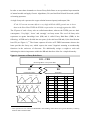
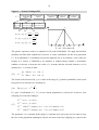
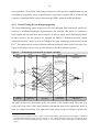
Modelling Expectations with GENEFER - an Artificial Intelligence approach by Eric Ringhut and [email protected] Stefan Kooths [email protected] Institut für industriewirtschaftliche Forschung Westfälische Wilhelms-Universität Münster Universitätsstr. 14-16, D - 48143 Münster, Germany http://www-wiwi.uni-muenster.de/iif June 2000 Abstract Economic modelling of financial markets means to model highly complex systems in which expectations can be the dominant driving forces. Therefore it is necessary to focus on how agents form their expectations. We believe that they look for patterns, hypothesize, try, make mistakes, learn and adapt. Agents’ bounded rationality leads us to a rule-based approach which we model using Fuzzy Rule-Bases. E. g. if a single agent believes the exchange rate is determined by a set of possible inputs and is asked to put their relationship in words his answer will probably reveal a fuzzy nature like: “IF the inflation rate in the EURO-Zone is low and the GDP growth rate is larger than in the US THEN the EURO will rise against the USD”. ‘Low’ and ‘larger’ are fuzzy terms which give a gradual linguistic meaning to crisp intervalls in the respective universes of discourse. In order to learn a Fuzzy Fuzzy Rule base from examples we introduce Genetic Algorithms and Artificial Neural Networks as learning operators. These examples can either be empirical data or originate from an economic simulation model. The software GENEFER (GEnetic NEural Fuzzy ExplorER) has been developed for designing such a Fuzzy Rule Base. The design process is modular and comprises Input Identification, Fuzzification, Rule-Base Generating and Rule-Base Tuning. The two latter steps make use of genetic and neural learning algorithms for optimizing the Fuzzy Rule-Base. 2 Contents 1. Introduction ........................................................................................................................ 3 2. A Genetic and Neural Fuzzy Rule-Base approach towards modelling expectations......... 5 3. Managing Fuzzy Rule-Bases with GENEFER .................................................................. 8 3.1. Input Identification..................................................................................................... 9 3.2. Fuzzification............................................................................................................. 10 3.3. Rule-Base Generating .............................................................................................. 11 3.3.1. Rule-Base Creating .......................................................................................... 12 3.3.2. Rule-Base Simplifying ..................................................................................... 16 3.4. Fuzzy Rule-Base Tuning.......................................................................................... 17 4.3.1. Genetic tuning .................................................................................................. 17 4.3.2. Neural Tuning (Error-Backpropagation).......................................................... 19 4. 3.5. Adaptability of the system in a changing environment............................................ 22 3.6. Key Facts of GENEFER for Economic Model Builders ......................................... 24 Summary and directions for further research................................................................... 24 References ................................................................................................................................ 26 3 1. Introduction Modelling expectations has always been a major endeavour for economists as well as for psychologists. In economics there is a variety of theories requiring explicit expectation modelling. During the course of this paper we refer in particular to financial markets because of the predominant influence of forecasts on asset market transactions. As financial markets keep on displaying phenomena such as bubbles, crashes, herd behaviour, contagion, GARCH effects or focal points we will continue to ask: What moves the asset prices? FARMER gives a first hint by stating: “... to have a good theory of how prices behave, we will need to explain the behaviour of the agents on whom they depend”1. The standard academic literature is still not very convincing about modelling expectation formation. Although agents face a pool of publicly available information which consists of past prices, trading volumes, economic indicators, political events, rumours, news, etc., “there may be many different, perfectly defensible statistical ways based on different assumptions and different error criteria to use them…”2. That is the point where the psychologists’ view comes into play. Some cognitive scientists believe that agents form ‘mental models’ of the world in order to deal with complex environments.3 They look for patterns, hypothesize, try, make mistakes, learn and adapt.4 In doing so they inductively form expectations.5 The attempt to model their underlying mental processes explicitly is challenging, but it “… helps to ensure that theorists are not taking too much for granted and that their theories are not vague, incoherent, or, like mystical insights, only properly understood by their proponents”6. In recent years, there is a growing literature about the use of Artificial Intelligence (AI) methods for modelling these ‘mental models’ and their adaptation to a constantly evolving economic environment. Several papers are about John Holland’s Classifier Systems7 and their applications to various economic problems.8 As discussed in section 2, this technique does not meet all our demands on an AI-based approach for modelling expectations. Therefore, we propose an alternative way to model the formation of expectations in a complex environment using Fuzzy Rule-Bases (FRB) as an operational representation of ‘mental models’. We divided the design process of such a FRB in four major 1 2 3 4 5 6 7 8 See Farmer (1999), p. 31. See Arthur (1995), p. 7. For an introduction on mental models see Johnson-Laird (1983). See Marengo/Tordjman (1996), p. 410. See Arthur (1994). See Johnson-Laird/Shafir (1993), p. 6. See Holland (1975). See for instance Vriend (2000); Arthur et al. (1996); Marengo/Tordjman (1996) and Beltrametti et al. (1997). 4 steps and apply Genetic Algorithms as well as Artificial Neural Networks in order to learn and tune FRBs from observed data. In section three these steps of modelling and training FRBs are described. We do so by following a typical FRB-design session with the software tool GENEFER (G E netic N E ural F uzzy ExplorE R ) which was developed for handling Neural- and Genetic-Fuzzy Rule-Bases and whose key features for model builders are highlighted in section 3.6. The papers closes with a glance at possible applications of GENEFER and some suggestions for further research. 5 2. A Genetic and Neural Fuzzy Rule-Base approach towards modelling expectations The ‘true model’ of the world economy or national economies or even their single subsystems (e.g. markets, industries or firms) is still to be found. The massive interaction between millions of heterogeneous agents is the source for complexity which is continuously challenging our understanding of the world we live and (trans)act in. Although we record stock and bond prices, interest rates, exchange rates and many more prices for more than a century, we still lack a commonly accepted theory explaining the formation of these prices. Especially in financial market research we see several competing theories who each seem appropriate to explain specific market phenomena. Recent research breaks away from the widespread idea of neoclassical market foundations and the assumption of homogenous rational agents who instantaneously discount new information into prices, so that no technical trading can offer any consistent speculative profits and let markets appear to be perfectly efficient. Homogeneity means mutual consistency of perceptions about the environment (one commonly shared ‘true model’) and allows for the representative agent framework. There is accumulating behavioural evidence against this rational view9 as well as theoretical objections like costs of gathering and processing information and transacting, bounded rationality of agents and indeterminacy of deductively formed expectations10.11 Real financial markets are characterised by heterogeneous agents, who have different motives to trade, different planning horizons12, different beliefs about the ‘functioning or driving forces of the market’ and future events that will affect their action today and influence tomorrow’s asset prices. Financial decision makers face theoretical (competing theories), empirical (spurious correlation) and operational (non-measurability of inputs) difficulties in identifying relevant input data. Therefore, they do not base their decisions on a uniform input data set nor on a single accepted theory (but rather on a mixture of theories, on technical analysis (chart analysis), on what their competitors do etc.). Despite all these problems agents have to form expectations when (trans)acting in financial markets. Since their expectations 9 10 11 12 See McFadden (1999), p. 75 onwards. George Soros, one of the most successful and therefore most famous traders, expressed his opinion about the standard academic theory as follows: “…this [efficient market theory] interpretation of the way financial markets operate is severely distorted. ... It may seem strange that a patently false theory should gain such widespread acceptance“. See Arthur (1995), p. 8. See Albin (1998). For an interesting discussion about the effect of different planning horizons see Olsen/Dacarogna/Müller/ Pictet (1992). 6 mainly determine the aggregate market outcome which they try to predict, expectations become self-referential and a rational deduction of the ‘true model’ becomes impossible. An agent cannot deductively form his expectations, since he needs to know others’ (privately held) expectations in order to form his own ones – consequently these are indeterminate.13 Even in the absence of informational deficits an agent might not be able to fully understand the complexity of a market or the costs of discovering the exact input-output relation in finite time exceed the benefits from it. Both, the limited information processing capability, that stems from the intrinsic data complexity, as well as the lack of information, bound the agents’ rationality. With respect to the case of non-measurability of others’ expectations, they face an absolute barrier to rationality. But of course we see agents forming expectations everyday. How do they do it? As we mentioned above, agents look for patterns or rules within the market. In doing so they mentally form a rule-based representation of the market’s functioning. These rules reflect their experiences and may be influenced by economic theory. This rule-based approach includes the expression of explicit (e. g. technical trading rules) as well as tacit knowledge. Due to agents’ bounded rationality these rules, however, should not be interpreted as exact mathematical functions but rather as a relationship between the agents’ interpretation of the input and output variables’ states. We contend that agents interpret these crisp states vaguely by associating them gradually with a limited number of linguistic terms (e. g. ‘low’, ‘medium’, ‘high’).14 An evolving economic environment continuously generates new observations which extend an agent’s experience. New observations might conflict with current knowledge so that there is a necessity to learn (by changing rules or the interpretation of crisp data). The conclusions we draw from the description above leads to the following list of demands on a realistic approach for modelling expectations: (D1) explicit knowledge representation ((theory-driven rules), model building) (D2) vague formulation of forecasts (bounded rationality) (D3) dependency upon experiences (ability to learn) 13 14 See Foley (1998), p. 53 onwards and for a beautiful explanation Arthur (1995), p. 3 onwards. This is opposed to classifier systems which usually interpret crisp data by means of crisp intervals (see fn. 8). 7 In order to meet these demands we choose Fuzzy-Rule Bases as an operational representation of mental models and apply Genetic Algorithms (GA) and Artificial Neural Networks (ANN) as learning operators. A single fuzzy rule expresses the vague relation between input(s) and output, like: IF the US current account deficit is very high AND the GDP growth rate is lower than in the Euro-Zone THEN the EURO is expected to rise strongly against the USD. The IF parts of such a fuzzy rule are called antecedents, whereas the THEN parts are their consequents. ‘Very high’, ‘lower’ and ‘strongly’ are fuzzy terms. The set of all fuzzy rules represents an agents knowledge base (KB) and is called Fuzzy Rule-Base (FRB) in the following. A FRB can be divided into two parts (i) the rule-base RB and (ii) the fuzzification base FB (see Figure 1).15 The former captures all rules as IF-THEN statements whereas the latter provides the fuzzy sets, which express the terms’ linguistic meaning as membership functions in the universes of discourse. We additionally assign a weight to each rule indicating its relative importance within the RB and therefore allow for a simple hierarchy. Figure 1: Structure of Fuzzy Rule-Bases KB = FRB Knowledge Base = Fuzzy Rule-Base FB RB Fuzzification Base Rule Base low medium high Input1 very low low medium high very high Input2 low medium high IF Input1 AND Input2 THEN Output low medium medium low very high high medium very low low high very high high low low low high medium medium high very low medium medium low low medium medium medium high medium medium Output 15 This separation is also realised in GENEFER’s data handling, which allows for a greater flexibility of linking different FBs to different RBs. 8 Both, FB and RB can be modified during an agent’s learning process. The GA-approach requires a suitable encoding of these objects in order to apply its genetic operators (selection, mutation, crossover). Transforming the FRB into an equivalent Artificial Neural Network opens it up to neural learning techniques (such as error-backpropagation). Whereas fuzzy systems account for (D1) and (D2), their combination with GA- and ANNtraining techniques meet all three demands. The use of Genetic and Neural Fuzzy Rule-Bases and their implementation in GENEFER is sketched in the next section. 3. Managing Fuzzy Rule-Bases with GENEFER GENEFER is a software for designing a FRB of the Mamdani multiple-input-single-output type. The primarily technical literature about fuzzy control proposes numerous ways of setting up a FRB. GENEFER does not focus on one of the many ways but separates the design process in four major steps (and thus offers the user to combine alternative methods): (i) identifying inputs, (ii) fuzzifying crisp input and output data (FB), (iii) generating a rule base (RB) and finally (iv) tuning the FRB.16 The design methods of each step can be run either in an inductive or in a manual (expert) mode. The former applies combinations of GA or ANN with Fuzzy Logic Controllers17 and requires a training data set of observations (TDS) for learning. GENEFER is equipped with a DESIGN NAVIGATOR that allows quick and easy navigation through the process of FRB-design. The description of each step below will show the respective DESIGN NAVIGATOR’s appearance. We will not explain the basics in fuzzy inference but only mention that we used t-norm operators for calculating the activation degree ADi of a single rule i and accumulated these degrees using the sum procedure [min(1, ∑ ADi )] in order to obtain a compositional activation degree. The fuzzy inference result can optionally be defuzzified by the (i) Centre of Maximum weighted by surface, (ii) Centre of Maximum weighted by significance, (iii) Centre of Gravity weighted by Surface or (iv) Centre of Gravity weighted by Significance. Since it is beyond our purposes here, we will also avoid to go into detail with GA and ANN and refer to the standard literature instead. We do not understand this paper as a user manual. We will rather highlight the most crucial features to model builders, in order to raise interest in applying GENEFER to economic simulations. 16 17 The modular design is strongly influenced by the work of Cordón/Herrera (1997). See Lin/Lee (1991), Lin (1994) and Cordón/Herrera (1997). 9 For the sake of better readability and easier access to mathematical notations, we list our frequently used indexes and variables below: j ∈ {1,…,J} Input index outt Output in t t ∈ {1,…,T} Period index Ai Antecedent of Rule i i ∈ {1,…,M} TDS Rule index Aij Fuzzy set of input j in Rule i Training data set Bi Output fuzzy set in Rule i p ∈ {1,…,P} Period index (only in 3.1.1.a) B = {B1,...,BNOut } Set of all output fuzzy sets n ∈ {1,...,N} injt Fuzzy set index Ai(injt) [Bi(outt)] Membership value of injt Input j in t Bi(outt) [Bi(outt)] Membership value of outt int = {in1t,...,inJt} Input vector in t outFRB(int) Crisp inference result 3.1. Input Identification GENEFER’s data interface uses an Excel 5 compatible file format with the following worksheet organisation: horizontally the worksheet is divided into the output range (first column) and the input range (following columns). The first row is designated for time series labels. The number of the following rows containing numerical data is equal to the number of periods. After importing data GENEFER offers three different ways to proceed. If the user has complete pre-knowledge about the relevant inputs he will choose the respective option in the DESIGN NAVIGATOR and select the desired time series. Otherwise he can apply GENEFER’s identification algorithm. If the user is completely or partially ignorant on the set of independent inputs, he will proceed along the tree items ‘none’ and ‘partial’ respectively. In the latter case preselected time series are definitely included in the final set of inputs before the user runs the FC/FS-identification algorithm. This algorithm iteratively eliminates unimportant and related inputs. In the first step it calculates J fuzzy curves (FC) for each input–output combination and determines the MSE between these curves and the observed output data. FC-Ranking in ascending order yields the most important input (lowest MSE). Each step will be closed by eliminating a FHUWDLQSHUFHQWDJH RILQVLJQLILFDQWLQSXWVKLJKHVW06(7KHIROORZLQJVWHSFRPELQHVWKH previously identified input with each remaining possible input and output to calculate (1⋅(N-1) fuzzy surfaces (FS). Sorting all FS according to MSE indicates the second most important input. Computation of these surfaces will proceed until the set of possible inputs is 10 empty. The FC/FS-algorithm is a computationally fast method to isolate an independent set of significant input variables of a complex, poorly defined, nonlinear system.18 3.2. Fuzzification As far as the previous step has been accomplished a variable’s fuzzification can be accessed directly via the DESIGN NAVIGATOR. Clicking on one of these variables opens the Fuzzification Dialog in Figure 2. Starting with a default FB this dialog allows the user to fuzzify each variable separately. The degree of granularity (number of fuzzy sets) or the type of fuzzy sets (triangular or gaussian) are not uniform but may differ for input(s) and output. As it is known from cognitive science, human beings are usually capable of distinguishing up to 7 significant classes.19 Therefore we restrict the number of fuzzy sets per variable. This may be either 3, 5 or 7. The fuzzification dialog assists the user in easily fuzzifying the output and the identified inputs. GENEFER displays the default fuzzification for all variables if the user has not specified a FB yet. The user may modify this by changing the settings in the displayed form below. These settings refer to the selected variable in ➀. The user determines the number of fuzzy sets in ➁ and their type in ➂. Grid ➃ shows the centres and widths but also allows for manual editing if this option is selected (deactivation of ➄). Additionally, a clustering algorithm is offered for which the required settings can be found in ➅ above the grid. This algorithm runs over all periods in the fuzzification interval ➆ and guarantees a minimum membership value (equal to the overlap in ➅) for each observation of the selected variable within this interval. Maximum and minimum values of the chosen variable within this interval are displayed in ➇. It is important to point to the ‘S-Shape (Border Sets)’ option ➈. In case of a new observation being outside the support of all fuzzy sets, this option helps avoiding the failure to generate an inference result.20 18 19 20 For a detailed description of the FC/FS-algorithm see Lin/Cunningham/Coggeshall (1996), pp. 65-71. In addition to their proposal all input time series are scaled within the unit interval in order to avoid distorted results due to significant differences in standard deviations. See Altrock (1995), p. 153 and Pedrycz/Gomide (1998), p. 67. Note that this failure cannot occur during the FRB-design process, since the interval for inductive learning can only be equal or part of the interval in the previous step. 11 Figure 2: Fuzzification Dialog 3 9 5 7 8 1 2 6 4 3.3. Rule-Base Generating The user’s decision about the granularity of input variables determines the maximum number J of possible rules MMax = ∏ Nj, which is equal to every possible combination of input fuzzy j=1 sets. A RB consisting of MMax rules will inevitably become intractable if the number of inputs increases. Therefore it seems advantageous to remove (or better not even create) all redundant rules. E. g. if an agent who distinguishes between a ‘low’, ‘medium’ and ‘high’ inflation rate and ‘weak’, ‘medium’ and ‘strong’ growth of GDP, has never experienced a combination of low inflation rate and strong growth of GDP, why should he have a rule for this case? 21 The DESIGN NAVIGATOR above shows the two major steps of the RB generating process which are described below. 21 See Legrenzi/Girotto/Johnson-Laird (1993), pp. 38 onwards. For those, who might ask what to do, if a new observation begets an unexperienced input value combination, we refer to section 3.5. 12 3.3.1. Rule-Base Creating Rule-Base Creating splits up in a descriptive and an approximate approach. They differ in the linguistic meaning of each fuzzy set when interpreting fuzzy rules. The descriptive approach is characterised by a uniform meaning of all fuzzy sets in all rules. If the second set of the third input appears in more than one rule, it always has the same meaning (e.g. medium) and is represented by the same membership function. Changing this function will consequently affect all rules that contain the respective fuzzy set. Hence there are no restrictions on economic interpretability of a descriptive FRB. In contrast to this, the approximate approach allows fuzzy sets to differ from rule to rule (free semantics). Whereas this may have advantages concerning the goodness of fit, it is not accessible to an economic interpretation. With respect to our purposes here, we do not consider the approximate approach in the following, but concentrate on the interpretable descriptive one.22 The designer of a FRB has to pay attention to two properties in order to obtain good results.23 The completeness property guarantees that the FRB is able to generate an inference result for each observation of input values in the TDS. The completeness property can be assigned to the FB and the RB. A FB is complete if the union of all fuzzy sets for each input variable covers the related universe of discourse. If it covers to a level of σ ∈ [0,1], the FB is called σcomplete. In contrast to this, a RB is called complete if it is able to generate an inference result for any input proposition. As we mentioned above this may lead to an unacceptable large number of rules if certain regions in the input space are not covered or can be excluded. Therefore we relax the RB completeness property by requiring each observation dt = (int, outt) in the TDS to be covered to a degree of at least CV(dt) ≥ ε > 0. The Covering Value CV is calculated as follows: (1) Ai (int) = min(Ai1 (in1t),…, AiJ (inJt)) (2) Ri (dt) = min(Ai (int), Bi (outt)) (3) CV(dt) = U Ri (dt) M i=1 M (4) CV(dt) = ∑ Ri (dt) i=1 22 23 We plan to test GENEFER’s forecast abilities and will, of course, include the approximate approach in order to evaluate if it shows better results than the descriptive one. See Pedrycz/Gomide (1998), ch. 10.6 and especially Gordón/Herrera (1997), pp. 377-380. 13 Equation 1 (2) is the compatibility degree between the ith rule’s antecedent (the ith rule) and the observation int (dt). Equation 3 is the generic Covering Value while the iterative nature of the evolutionary RB creating procedure (see below) requires its modification to equation 4. The second property is the consistency of a FRB. A Rule-Base (not FRB!) is called consistent if it does not contain contradictions. A contradiction arises when two or more rules have the same antecedents but not the same consequent. In FRBs there is a need to relax the consistency requirement due to fuzzy modelling. It is the essence of fuzzy modelling that a crisp observation may be consistent with more than one fuzzy rule, which may of course differ in their consequents. But this does not necessarily imply contradictions, just like there is no contradiction in stating that a person is tall to a degree of 0,9 and very tall to a degree of 0,25. In order to avoid contradictions in FRBs we will apply the concepts of positive and negative observations. An observation is regarded positive for a fuzzy rule if it matches its antecedent and consequent with a compatibility degree Ri(dp) greater than or equal to ω : (5) TDS + S (Ri) = {dp ∈ TDSp Ri (dp) ≥ ω} In case of matching the antecedent but not the consequent the observation is considered negative for the rule. TDSp-(Ri) = {dp ∈ TDSp Ri (dp) = 0 and Ai(inp) > 0} (6) With respect to this relaxation we call a FRB consistent if it provides a sufficient small number of negative observations, measured as the percentage k of positive observations. GENEFER offers three options to create a FRB as shown in the DESIGN NAVIGATOR above. The two first inductively create a FRB by using the information inside the TDS. The third one allows for manual creation of fuzzy rules in order to make use of expert knowledge. a) evolutionary The evolutionary method is an iterative process to generate a complete and consistent RB for all observations in the TDSp. It is therefore necessary to carefully select these observations so that they cover all possible input combinations. One step encompasses the four following substeps: • Creation of a candidate RB matching all observations within the TDSp. • Evaluation of all candidate rules according to a fitness function. • Copying the best (the fittest) rule to the generated RB and clearing the candidate RB. 14 • Removal of all observations in the TDSp for which CV(dt) > ε A candidate rule is created by linking those fuzzy sets that yield the highest membership value for the current observation’s variables values. A TDSp of P observations will therefore lead to a candidate RB of P or less fuzzy rules, since doubles are excluded. The consecutive evaluation uses a multicriterion fitness function which considers the following criterions: (7) High Frequency Value: P ∑ Ri (dp) TDS(Ri) (8) = p=1 P High Average Covering Degree Over Positive Observations: ∑ G (Ri) = Ri(dp) TDSp, +(Ri) dp∈TDSp, +(Ri) (9) Small Negative Example-Set: if TDSp-(Ri) ≤ k⋅TDSp, +(Ri) 1 gn(R i ) = 1 TDSp-(Ri) − k⋅TDSp, +(Ri) + exp(1) otherwise (10) Fitness function: F(Ri) = TDS(Ri)⋅G - (Ri)⋅gn(R i ) The best rule, the one with the highest fitness value, is copied to the generated RB. This generated RB is then used to compute the Covering Value for all dp ∈ TDSp (see Equation 4) and all observations whose CV is greater than or equal to ε will be removed. The candidate RB is cleared for the next step which runs over the reduced TDSp. This process terminates when TDSp = ∅. b) neural As an alternative to the evolutionary procedure GENEFER offers an unsupervised competitive neural learning algorithm for detecting rules in a given set of observations.24 The algorithm works as follows: At the beginning of the learning process all antecedents i are 24 For the underlying feature-map-algorithm see Kohonen (1988), ch. 5, particularly p. 132. 15 virtually connected with all consequent terms. “Virtually connected” means that there is a potential connection between each antecedent i (i = 1,...,MMax) and each consequent set q (q = 1,...,NOut) with an initial connection weight of zero (wiq = 0 ∀ i). Presenting a training pattern dt allows to compute the activation degree for each antecedent Ai(int) and the membership value for each fuzzy set q of the output variable Bq(outt). These values are used to adapt the connection weights by means of the following learning rule: (11) ∆wiq = Bq(outt)⋅[−wiq + Ai(int)] At the end of the learning procedure (after a given fixed number of training patterns) the connection with the maximum connection weight of each antecedent is kept and all others are removed. c) manual GENEFER’s expert mode allows to (re-)design the complete RB or parts of it including the rule weights vector manually (setting a rule weight to zero deactivates the rule). If no RB has yet been created the program delivers an initialized normalized RB by generating all MMax antecedents with the output’s mid-term as the default consequent. This basic RB can then be used as a starting point for further individual modelling. By setting influence factors inffj for each input variable j the antecedents of an initialized RB can be connected automatically to the respective consequent sets. Influence factors reflect ceteris paribus reasoning and are represented by integers reaching from –3 to 3 (-3 means strong negative influence, zero means no influence and 3 means strong positive influence). In the automatic RB-connection procedure each input and output fuzzy term is identified by its relative position (RP) towards the respective mid-term. E.g. the linguistic term set {very low, low, medium, high, very high} is represented as {-2,-1,0,1,2}. Given the user defined influence factors for all inputs the relative position RP(Bi) of the consequent set in any rule i is found as follows: (12) 1 J RP(Bi) = trunc3 ∑inffj⋅RP(Aij) ∧ RP(Bi) ≥ RP(B)min ∧ RP(Bi) ≤ RP(B)max j=1 16 3.3.2. Rule-Base Simplifying Although the previous step already provides a valid FRB, the user can try to improve its performance. The RB-creating process might lead to a larger amount of rules than necessary. Redundant rules occur due to overlearning, when some observations in the TDS have a higher covering degree than the desired one.25 The purpose of simplification is to remove these redundant rules by applying genetic operations on a population of encoded RBs. A RB is encoded as a binary string C of length M which can be regarded as a sequence of switches that either turn a rule on (digit 1) or off (digit 0). A string only containing the digit 1 represents the created RB of the previous step. All other individuals in the population are initialised randomly. The population is of constant size K with k ∈ {1,...,K}. The user may choose between three selection procedures: (i) Stochastic Universal Sampling (SUS) (rang-based), (ii) SUS (fitness-proportional) and (iii) Tournament Selection to determine the individuals for the mating pool. The activation of the elitist selection option guarantees the survival of the fittest individual in the next population. The offspring population is created by the classical binary multipoint crossover and uniform mutation operators. The fitness of one individual Ck is determined by its MSE over the TDS. The lower this error the better the individual. Since there is a need to fulfil the completeness requirement, the fitness value has to be modified in case of a completeness violation. We ensure this by requiring that each observation in the TDS has a CV (equation 3) of greater or equal to τ. The completeness property for Ck over the complete TDS is defined as training-set completeness degree: (13) TSCD(Ck, TDS) = dt∈TDS CVCk (dt) The following fitness function penalises the fitness value if the training-set completeness degree is violated: (14) MSE(Ck) F(Ck) = 1 ∑(outt)2 2 d ∈TDS if TSCD(Ck, TDS) ≥ τ otherwise t It is important to note that GENEFER does not delete any redundant rules. The procedure of simplifying attempts to improve the performance of a previously created FRB by switching 25 See Gordón/Herrera (1997), p. 391. 17 single rules on and off. As a result we obtain a binary code of switches that is linked to the generated FRB. This linkage might possibly yield a reduced FRB. Nevertheless the user is always able to work with the generated one by (re)-activating all rules (turning on all switches). 3.4. Fuzzy Rule-Base Tuning RB-simplifying and FRB-tuning both aim at improving the system’s forecast performance. Whereas RB-simplifying uses a given FB in order to refine the RB, the FRB-tuning focus is on adjusting the fuzzy sets parameters. The current fuzzification of input(s) and output might not be as suitable as it could be regarding the goodness of fit. The search space is limited to the fuzzy sets’ centres and widths without changing their a-priori defined type and the degrees of granularity. GENEFER offers two popular tuning algorithms for fuzzy systems: genetic and neural tuning (error-backpropagation). In the latter case the FRB is transformed into a Neural-FRB with a given topology. We do not apply explicit structural learning (changing the network’s topology) but focus on parametric learning. 4.3.1. Genetic tuning The genetic approach requires a suitable representation of the input and output fuzzification. We encode the complete FB as a sequence of real 3-tupels such as (fl, fc, fr) with fl (fr) as a fuzzy set’s left (right) border and fc as its centre. The complete encoding C of all fuzzified variables (= FB) is the object to be genetically modified. The encoded fuzzification of one input variable j contains 3⋅Nj elements c, so that the encoded FB is a sequence of 3⋅Nj⋅Nout⋅J elements. The encoded current fuzzification as well as randomly initialised individuals form the starting population in the first generation t. Initialisation and genetic operations take place in a specified search space. The structure of C as well as the search space for fuzzy parameter adaptation are shown in figure 3. 18 Figure 3 Genetic Tuning of FB C= Fuzzification Fuzzification Fuzzification Fuzzification Fuzzification ;...; ; ;...; Input 1 Input j Input J-1 ; Input J Output Aj1 Ajn AjN c , c , c c1, c2, c3 ;...; 3n-2 3n-1 3n ;...; c3N-2, c3N-1, c3N fl fc Ajn 1 fr fc-fl fc-fl fl ∈ [fll , flr] = l - 2 , fl + 2 fr-fc fc ∈ [fcl , fcr] = flr , fc + 2 fr-fc fr ∈ [frl , frr] = fcr , fr + 2 fll fl flr=fcl fc fcr=frl wl wr fr frr inj The genetic operators need to be adapted to real coded individuals. We apply non-uniform mutation and Max-Min arithmetical crossover to create individuals for the next generation t+1. If an individual C is randomly selected for mutation one of its elements c (one of the two borders or a centre) is identified to be mutated. A random binary number α determines whether to increase or decrease the value of c. Assume that the selected element cn to be mutated to cn’ is a centre fc then: (15) cn + ∆(t,fcr − cn) cn’ = cn - ∆(t,cn − fcl) if α = 1 if α = 0 The result of the function ∆(t, y) is a value in the range [0, y] and the probability of the result being close to 0 increases in t according to: t b (16) ∆(t, y) = y (1 − r (1 − T) ) If a pair of individuals (CP1, CP2) in the current population is selected for crossover, four offspring are created according to : C1t+1 = a CP1 + (1−a) CP2 C2t+1 = a CP2 + (1−a) CP1 (17) C3t+1 with c 3 = min(cP1, cP2) ∀ cP1 ∈ CP1 and cP2 ∈ CP2 C4t+1 with c 4 = max(cP1, cP2) ∀ cP1 ∈ CP1 and cP2 ∈ CP2 t+1 t+1 The parameter a is a constant in the range [0,1] and has to be set by the user. In order to keep the size of the population unchanged, only the two best of the four offspring are copied in the 19 next population. We used the same fitness function as in the previous simplification step for evaluating the population. Since each individual C represents a complete FB, it is linked to the created (or simplified) RB in order to determine the FRB’s output for MSE calculation. 4.3.2. Neural Tuning (Error-Backpropagation) The neural FRB-tuning option makes use of the fact that both fuzzy and neural systems are based on a distributed knowledge representation. On principle, this allows to transform a fuzzy system into an equivalent neural network, in order to apply neural learning procedures to fuzzy systems. For this purpose we interpret the FRB as a hybrid neuro-fuzzy system (connectionist fuzzy control system) according to the basic technology presented by Lin and Lee.26 This approach uses a layered feedforward neural network with a total of five layers (see Figure 4). Each layer carries out a specific function in the fuzzy inference process. Figure 4 Neural fuzzy system with two input variables layer 1 layer 2 layer 3 layer 4 layer 5 basic input nodes input term nodes antecedent nodes consequent nodes/ output term nodes defuzzifying node/ output node rule base/ inference engine fuzzy AND fuzzy AND fuzzy AND fuzzy AND crisp value of input 2 fuzzy AND fuzzy AND limit. SUM limit. SUM limit. SUM limit. SUM crisp forecast value crisp value of input 1 fuzzy AND limit. SUM fuzzy AND fuzzy AND signal distribution fuzzification of the input values aggregation conclusion/ accumulation defuzzification of the output value The nodes in layer one (basic input nodes) are sensors to the outside world. Their task is to receive the crisp values of the input variables and transmit them to the appropriate nodes in layer two (input term nodes). The input term nodes carry out the fuzzification function for 26 See Lin/Lee (1991) und Lin (1994). A good overiew of hybridizing neural and fuzzy technologies is delivered by Nauck/Klawonn/Kruse (1994), pp. 231 onwards. A very concise description of the basic concepts of neural networks can be found in Buckley/Feuring (1999), ch. 3. For details in neural technologies see Hecht-Nielsen (1991). 20 each input. Every basic input node is connected with all input term nodes of the respective input variable which represent the different linguistic terms.The parameters used for characterizing the membership functions (centers and widths) can be interpreted as link weights between layer one and two. After calculating the degrees of membership for all linguistic input terms the layer two nodes propagate this result to the next layer whose nodes represent the antecedents of the RB. Each of them computes the activation degree of the respective rule by means of the fuzzy AND operator. All cross term combinations between all inputs are represented in the aggregation layer, so the number of links of each conditional node to the anterior nodes equals the number of inputs. Since the aggregation procedure works with unweighted input data (i.e. degrees of membership of the concerned terms) the link weights between layer two and three are constant and equal to one. Each node at layer four (consequent nodes in the conclusion/accumulation layer) corresponds to one linguistic term of the output variable (output term nodes). Each of these nodes receives the degrees of application of those conditional nodes which point at the respective consecutive term represented by the considered node at layer four. Optionally the activation degrees can be weighted by means of link weights between the layers three and four. A link weight of zero means that the respective rule has been deactivated. The third and fourth layer constitute the connectionist inference engine which embodies the complete RB of the equivalent fuzzy system. The single node in the fifth layer (output node) defuzzifies the fuzzy inference result and delivers the crisp forecast value. The link weights between layer four and five represent the centers and widths of the fuzzy sets that represent the linguistic terms of the output variable. The efficiency of a neural network with a given topology and node functionality only depends upon the values of the link weights which determine how the node output of layer s is propagated to the subsequent nodes in layer s+1. The knowledge of a neural network is therefore embodied in the values of the link weights. The fact that the complete functionality of the fuzzy inference process is represented equivalently by the neural network allows the application of neural learning methods for FRB-tuning. GENEFER’s neural learning method is a modified error-backpropagation procedure (MEBP). The starting point of the learning process is the mean squared error over the TDS: (18) 11 T 2 MSE = 2 T ∑(outFRB(int) – outt) t=1 21 The learning procedure aims at minimizing the error function (18) by finding the weight vector which minimizes MSE. The underlying idea of error-backpropagation is that all nodes of the network (not only the output node) are responsible for the network error due to their influence on the signal propagated through the network. During the training phase the signal’s direction is reversed, so that each learning round starts at the output node with the network error being fed into the network. This error signal is then backpropagated layer by layer until it reaches the basic input nodes. Hereby, the global network error is distributed over all relevant nodes. Since each node’s signal can only be changed by adjusting its link weights these are the object of the learning process. The adjustment of each weight w is proportional to its marginal influence on the network error. This method implies a linear approximation of the error function in the environment of the current weight values. (19) ∆w = –µ ∂MSE ∂w If we plot the network error as a function of all link weights we get a mountain-like error surface in which equation (19) describes the steepest way down with the exogenous learning rate µ determining the stride (gradient descent algorithm). We omit further details and formulas of the parameter adjustment procedures here,27 but it should be noticed that they depend on the fuzzy types, the fuzzy AND operator and the rule weighting option. The neural learning operations described so far reflect the standard error-backpropagation algorithm (EBP) whose results do not necessarily account for the specific needs of a fuzzy rule base. Sometimes, it is suitable to exclude the adaptation of certain parameters or to restrict their adjustment ranges in order to keep the whole fuzzy system in a sound state. Otherwise it might happen that the EBP-algorithm ruffles the FB leaving us with a degenerated system that lacks economic interpretability (e. g. negative or extremely small fuzzy set widths or fuzzy set centres that can hardly be distinguished from each other). In these situations special MEBP-filters intervene in order to get a differentiated fuzzification of the relevant crisp data intervals (e. g. by ensuring a minimum overlap of adjacent fuzzy sets). The underlying idea of the adjustment-filters is the formulation of various criteria for a sound FRB and to inhibit the learning process whenever one (or more) of these criteria is running the risk to be violated. 27 See Kooths (1998), section 2.5.3.4. 22 The MEBP-algorithm was especially designed for applying a given FRB to observations which might differ considerably from the training data set. In this case GENEFER finds itself on „virgin soil“ which might be due to a radical change within the economic system. „Virgin soil“ appears whenever the fuzzy sets do not cover the relevant crisp interval in an adequately differentiated way and/or whenever the relevant crisp values lie in the border regions of the fuzzified interval. 3.5. Adaptability of the system in a changing environment This section is about GENEFER’s application in an economic simulation. As we have mentioned in section 2, there is a need to guarantee the system’s adaptability to a changing environment due to the learning ability of agents. The major steps in the design process reveal some useful procedures which can be used for our purposes here as well. Nevertheless GENEFER’s spectrum must be extended. The software must allow for exploitation of agents’ existing knowledge as well as for exploration of new knowledge if the observed data conflict with the agents’ expectations. The two tuning procedures in the section above could serve as means for exploitation of knowledge. E. g. an agent who is used to an inflation rate between 1% and 2% will (sooner or later) change his opinion about the meaning of ‘high’, if the inflation rate exceeds his experienced top level. The tuning routines adapt the fuzzification of input(s) and output according to a changing economic environment. They check for the existence of a better FB, that leads to an improved forecast performance. The user specifies a time interval in which no tuning occurs. If he wants to prohibit tuning, he will set this interval equal to the simulation interval – if he wants agents to learn continuously, the interval is set to one. In contrast to this, exploration procedures search for new rules without adjusting the FB. As we mentioned above the generation process creates a FRB, which covers all observations in the TDS but cannot guarantee to provide a fuzzy rule for all possible values of input-output combinations. In the case of a missing rule or poor covering of existing rules28, GENEFER offers two ways to explore the rule search space. The first one is to continuously replace an agent’s FRB after a user-specified number of simulation periods. GENEFER will therefore generate a new FRB on (i) an enlarged TDS including all new observations or (ii) a TDS of constant size including a user specified number of observations (moving window). The 28 A poor covering may occur with gaussian fuzzy sets, which always yield positive membership values but not necessarily significantly different from zero. 23 technical realisation might exceed computational capacity when the number of agents increases and/or when they are forced to replace their FRB quite frequently. Additionally one cannot exclude the case of false inference, if an uncovered observations occurs during the interval of unchanged FRB. For that reason, we introduce a second procedure, which allows to generate a new rule in case of a new observation, for which no forecast value can be inferred. If there has never been an observation of low inflation rate differential and high unemployment rate differential so far, there will probably be no rule covering such an observation. What should an agent expect about the exchange rate (assume that is the one to predict)? Will he throw dices to find out? Certainly not. We assume that such an agent will try to derive a new rule (and therefore a forecast result) by using his current knowledge. Let us consider an agent with the FRB in Figure 1 on page 7, who experiences a low inflation rate differential and a high unemployment differential. Let us also assume that none of his rules covers the observed data, so that no result can be inferred. The agent will then compare the existing rules’ antecedents with the observed input data in order to identify the most similar ones. If we index the fuzzy sets according to their position, we can encode the FRB as: IF Inflation rate differential AND Unemployment rate differential THEN 1 3 1 5 2 1 3 5 1 2 3 3 3 1 2 2 2 3 3 3 ¼86' 2 3 1 3 1 2 2 1 2 2 We compute the sum of the squared distance between each index of the new antecedent (1,4) and the ones for all antecedents in the FRB above for each rule. The lowest value yields the rule(s), which we regard as most similar. These are the first two in our example (02 + 12 = 1). The agent has to decide whether to expect the first rule’s consequent or the second one’s. We calculate the mean value and round the result, which will yield ‘high. The following rule will be added to the agent’s current FRB. 1 4 3 If the observed output at the end of this simulation period matches the newly appended rule’s consequent, it will be kept unchanged. If this is not the case, GENEFER will replace the consequent fuzzy set by the one yielding the highest membership value for the observed outcome. Therefore, an agent tends to expect what he has learned from observations so far. 24 3.6. Key Facts of GENEFER for Economic Model Builders GENEFER is not limited to a specific type of economic models. It can be implemented in: • macro-level simulations using a single FRB for modelling the representative agent’s or dominant market expectations (e. g. Dornbusch’s exchange rate model, Laidler’s monetarist business cycle model) • micro-level simulations for multiple-agent modelling with multiple FRBs giving room for analysing the interaction of heterogeneous expectations (see examples in fn. 8) The key AI-related features for expectation design are • 3 ways to set up a Knowledge Base consisting of fuzzy rules, which account for agents’ bounded rationality and allow for interpretability of the FRB inference result. • to modify this FRB in order to improve performance concerning a training data set (offline) or to model learning processes during a simulation (online). The modification includes the introduction of new fuzzy rules (exploration of knowledge) as well as the tuning of existing rules (exploitation of knowledge). • a huge flexibility in adapting the system’s behaviour to specific purposes. The user can set the agents’ inputs by default or let GENEFER learn which inputs are the most significant. He can define each rule in a FRB or let GENEFER learn a RB or even a combination of both. As far as simulation purposes are concerned the frequency to tune, simplify or even replace the FRB can be set individually for each agent. GENEFER comes with COM-server functionality giving access to those FRB-design related methods needed for the implementation of all features mentioned above. The user is therefore free to choose any preferred programming language for his computational economic simulations. 4. Summary and directions for further research In this paper we propose a new AI-based technique for modelling expectations. This technique combines fuzzy systems as a representation of knowledge bases with Genetic Algorithms (GA) and Artificial Neural Networks as learning operators. We describe their synthesis and present the software GENEFER (GEnetic NEural Fuzzy ExplorER). Economic model builders can implement GENEFER in their simulations via a COM-interface and make 25 use of its fuzzy inference and learning routines. Nevertheless it may also be used for pure forecasting purposes on empirical data. We are currently testing GENEFER’s performance in forecasting financial time series. The development of self-documenting-business-cycle-indicators is on our research agenda for the near future. GENEFER’s modular architecture gives room for further combinations of AI techniques. We plan to apply GA in order to evolve a population of Fuzzy Rule-Bases and therefore reduce the amount of exogenous parameters, e.g. the learning rate. 26 4GHGTGPEGU Altrock, C. v. (1995), Fuzzy Logic, Band 1: Technologie, 2nd edition, Munich. Arthur, W. B. (1994), Inductive Reasoning and Bounded Rationality, SFI Paper 94-03-014, http://www.santafe.edu/arthur/Papers/Papers.html. Arthur, W. B. (1995), Complexity in Economic and Financial Markets, http://www.santafe.edu/arthur/Papers/Papers.html. Arthur, W. B. / Holland, J. H. / LeBaron, B. / Palmer, R. / Taylor, P. (1996), Asset Pricing under endogenous expectations in an Artificial Stock Market, SFI Paper 96-12-093, http://www.santafe.edu/sfi/publications/96wplist.html. Beltrametti, L. / Fiorentini, R. / Marengo, L. / Tamborini R. (1997), A learning-to-forecast experiment on the foreign exchange market with Classifier System, in: Journal of Economic Dynamics & Control, vol. 21, pp. 1543-1575. Buckley, J. J. / Feuring, T. (1999): Fuzzy and Neural: Interactions and Applications, Heidelberg/New York. Cordón, O. / Herrera, F. (1997), A three stage evolutionary process for learning descriptive and approximate Fuzzy-Logic-Controller Knowledge Bases from examples, in: International Journal of Approximate Reasoning, vol. 17, pp. 369-407. Farmer, J. Doyne (1999), Physicists attempt to scale the ivory towers of finance, in: Computing in Science & Engineering. Foley, Duncan K. (1998), Introduction, in: Barriers and Bounds to Rationality – Essays on Economic Complexity and Dynamics in Interactive Systems, Albin, Peter S., Princeton University Press, Princeton, New Jersey. Hecht-Nielsen, R. (1991): Neurocomputing; Reading, Mass. Holland, J. H. (1975), Adaptation in natural and artificial systems, University of Michigan Press, Ann. Johnson-Laird, P. N. (1993), Mental Models, Cambridge University Press, Cambridge/MA. Johnson-Laird, P. N. / Shafir E. (1993), The interaction between reasoning and decision making: an introduction, in: Cognition, vol. 49, pp. 1-9. Kohonen, T. (1988): Self-Organisation and Associative Memory, 3rd ed., Berlin. 27 Kooths, S. (1998): Erfahrungsregeln und Konjunkturdynamik - Makromodelle mit NeuroFuzzy-generierten Erwartungen; Frankfurt/Main u.a.O. Legrenzi, P. / Girotto, V. / Johnson-Laird, P. N. (1993): Focussing in reasoning and decision making, in: Cognition, vol. 49, pp. 37 – 66. Lin, C. T. (1994): Neural Fuzzy Control Systems with Structure and Parameter Learning; Singapore. Lin / Cunningham / Coggeshall (1996), Input variable identification – Fuzzy curves and fuzzy surfaces, in: Fuzzy Sets and Systems, vol. 82, pp. 65-71. Lin, C. T. / LEE, C. S. G. (1991): Neural-Network-Based Fuzzy Logic Control and Decision System; in: IEEE Transactions on Computers, Vol. 40, No.12 (Dec. 1991). Mamdani, E. H. / Assilian, S. (1975): An Experiment in Linguistic Synthesis with a Fuzzy Logic Controller; in: International Journal of Man-Machines Studies, Vol. 7, pp. 1 - 13. Marengo, L. /Tordjman, H. (1996), Speculation, Heterogeneity and Learning: A Simulation Model of Exchange Rate Dynamics, in: Kyklos, vol. 49, p. 407-438. McFadden, D. (1999), Rationality for Economists ?, in: Journal of Risk and Uncertainty, vol. 19 (1/3), pp. 73-105. Nauck, D. / Klawonn, F. / Kruse, R. (1994): Neuronale Netze und Fuzzy-Systeme Grundlagen des Konnektionismus, Neuronaler Fuzzy-Systeme und der Kopplung mit wissensbasierten Methoden; Braunschweig/Wiesbaden. Olsen, R. B. / Dacrogna, M. M. / Müller, U. A. / Pictet, O. V. (1992), Going Back to the Basics – Rethinking Market Efficiency, O & A Working Paper 1992-09-07, http://www.olsen.ch/library/research/oa_working.html. Pedrycz, W. / Gomide, F. (1998), An Introduction to Fuzzy Sets – Analysis and Design, MIT Press, Cambridge, Massachusetts, London. Vriend, Nicolaas J. (2000), An illustration of the essential difference between individual and social learning, and its consequences for computational analyses, in: Journal of Economic Dynamics & Control, vol. 24, pp. 1-19. Zimmermann, H.-J. (1991): Fuzzy Set Theory - and Its Applications, 2nd ed., Boston et. al.