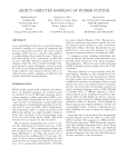
1
Object-oriented modelling of virtual-labs for
education in chemical process control
Carla Martin ∗, Alfonso Urquia, Sebastian Dormido
Dept. Informática y Automática, UNED, Juan del Rosal 16, 28040 Madrid, Spain
Abstract
Easy Java Simulations (Ejs) and Sysquake are two software tools specifically intended for implementation of virtual-labs. They allow easy definition of the virtuallab view (i.e., the model-to-user interface). However, the model definition capabilities
and the numerical solvers provided by these tools are not the state-of-the-art.
On the other hand, the use of the object-oriented modelling language Modelica
reduces considerably the modelling effort and permits better reuse of the models. Modelica is supported by the state-of-the-art simulation environment Dymola.
Nevertheless, Modelica does not provide the interactive capabilities required for
virtual-lab implementation.
The approach proposed in this manuscript is to combine the best features of each
tool. Ejs and Sysquake capability for building interactive user-interfaces composed
of graphical elements, whose properties are linked to the model variables. Modelica
capability for physical modelling and Dymola capability for simulating DAE-hybrid
models. This novel approach has been successfully applied to set up virtual-labs for
control education.
Key words: control education, virtual laboratory, interactive simulation, chemical
Preprint submitted to Elsevier Science
27 January 2006
process control, object-oriented modelling, Modelica
1
Introduction
Virtual-labs are effective educational tools for training of process engineers
and plant operators. They are distributed environments of simulation and
visualization tools, intended to illustrate some relevant properties of a system.
Virtual-labs are composed of: (1) the interactive computer simulation of the
system’s mathematical model; and (2) a narrative that provides information
about the system and the use of the virtual-lab.
Interactive computer simulations provide a flexible and user-friendly method
to define the experiments to be performed on the mathematical model. Interactive simulations allow the user to design and perform his own simulation
experiments. As a result, the user becomes an active player in his own learning
process, which motivates him to learn.
Typically, virtual-lab programming includes the definition of the mathematical
model and the virtual-lab view. The virtual-lab view is the user-to-model interface. It is intended to provide a visual representation of the model dynamic
behavior and to facilitate the user’s interactive actions on the model.
The model behavior can be represented in different ways. For instance, plotting
the model variables against each other and by means of animated schematic
diagrams of the system. In addition, linear systems can be described using
∗ Corresponding author. Tel.: +34 913988253.
Email address: [email protected] (Carla Martin).
2
pole-zero diagrams and frequency response diagrams (i.e., Bode and Nyquist
diagrams).
User’s actions on the model can be performed by manipulating different elements of the view, such as buttons, sliders, check-boxes and certain graphic
elements of the model schematic diagram. The graphical properties of the view
elements are linked to the model variables, producing a bidirectional flow of
information between the view and the model. Any change of a model variable
value is automatically displayed by the view. Reciprocally, any user interaction with the view automatically modifies the value of the corresponding
model variable.
1.1 Types of interactivity
User’s actions on the model are performed according to certain rules. Two
approaches are discussed next: runtime interactivity and batch interactivity.
Runtime interactivity allows the user to perform actions on the model at any
time during the simulation run. He can change the value of the model inputs,
parameters and state variables, perceiving instantly how these changes affect
to the model dynamic. An arbitrary number of actions can be made on the
model during a given simulation run.
In the case of the batch interactivity, the user’s action triggers the start of the
simulation, which is run to completion. During the simulation run, the user is
not allowed to interact with the model. Once the simulation run is finished,
the results are displayed and a new user’s action on the model is allowed.
3
1.2 Virtual-lab implementation software
Several virtual-lab packages, conceived to illustrate some selected topics in
automatic control, have been implemented. For instance, ICTools and CCSDEMO (Johansson et al., 1998; Wittenmark et al., 1998) are two packages
developed at the Dept. of Automatic Control, Lund Institute of Technology. In both cases, the virtual-labs are implemented using Matlab/Simulink
(http://www.mathworks.com/), a general-purpose simulation environment supporting the graphical block diagram modelling. As Matlab/Simulink is not specially suitable for interactive simulation, the development of new modules requires a considerable effort.
In addition, there are software tools specifically intended for implementation
of virtual-labs. These tools: (1) provide their own procedures to define the
narrative, the model and the view of the virtual-lab; (2) guide the virtual-lab
programmer in these tasks; and (3) automatically generate the virtual-lab executable code. Easy Java Simulations (http://fem.um.es/Ejs/) and Sysquake
(http://www.calerga.com/) are two of these tools.
A strong point of these tools is that they allow easy definition of the virtual-lab
view. Easy Java Simulations (hereafter cited as Ejs) provides a complete set
of interactive graphic elements which are ready to be used, in a simple dragand-drop way, to compose the view. Sysquake supports built-in functions to
include in the view different types of interactive plots and interactive graphic
elements (i.e., radio-buttons, sliders, dialog boxes, etc.).
However, the model definition capabilities and the numerical solvers provided
by these tools are not the state-of-the-art. They support the block diagram
4
modelling. This modelling paradigm requires of explicit state models (i.e.,
ordinary differential equations) and the computational causality of the model
must be explicitly set (i.e. the blocks have a unidirectional data flow from
inputs to outputs).
These restrictions do not facilitate the model reuse and they strongly condition
the modelling task, which requires a considerable effort. For instance, dummy
dynamics need to be introduced in the model to avoid the establishment of
systems of simultaneous equations. The model programmer has to manipulate the model to transform its equations to the form of ordinary differential
equations (ODE).
As a consequence, the modelling and simulation capabilities supported by
these tools are not the best possible ones for describing the large models used
in the physical-chemical field.
1.3 Contributions of this paper
The physical modelling paradigm, supported by the object-oriented modelling
languages, is an attractive alternative to the block diagram modelling (Aström
et al., 1998). Object-oriented modelling languages support a declarative description of the model, based on equations instead of assignment statements.
The computational causality is not included in the model. Thus, a model can
adapt to more than one data flow context. The modelling knowledge is represented as differential, algebraic and discrete equations that may change by
being triggered by events (i.e., hybrid-DAE models).
Some examples of object-oriented modelling languages are EcosimPro, gPROMS
5
and Modelica. The Modelica language (http://www.modelica.org/) has been
designed by the developers of the object-oriented modelling languages Allan,
Dymola, NMF, ObjectMath, Omola, SIDOPS+, Smile and a number of modelling practitioners in different fields. It is intended to serve as a standard
format for the external model representation, so that models arising in different engineering fields can be exchanged between tools and users. Modelica language is supported by the Dymola modelling environment (http://www.dynasim.se/).
The use of the Modelica language reduces considerably the modelling effort
and permits better reuse of the models. However, Modelica does not provide
the interactive capabilities required for virtual-labs implementation.
The approach proposed in this manuscript is to combine the best features of
each tool. Ejs and Sysquake capability for building interactive user-interfaces
composed of graphical elements, whose properties are linked to the model variables. Matlab/Simulink capability for modelling of automatic control systems
and for model analysis. Modelica capability for physical modelling, and finally
Dymola capability for simulating hybrid-DAE models. This software combination approach is discussed for implementation of virtual-labs with runtime
interactivity (Section 2) and with batch interactivity (Section 3).
This novel approach has been applied to the implementation of a set of virtuallabs. Their topic is the open-loop dynamic and the control of three process
units widely used in the chemical industry: a double-pipe heat exchanger (Section 4), an industrial boiler (Section 5) and a batch chemical reactor (Section
6).
The objective of these virtual-labs is to help the students to: (1) understand
the behavior of the plant non-linear models; (2) apply some linearization tech6
niques; (3) analyze the plant linearized models using zero-pole, Bode and
Nyquist diagrams; and (4) design the PID, lead and lag compensators required to control the processes.
2
Implementation of virtual-labs with runtime interactivity
Ejs is an open source, Java-based software tool intended to implement virtuallabs with runtime interactivity (Esquembre, 2004). It can be freely downloaded
from the Ejs’ web-site (http://fem.um.es/Ejs/).
Ejs guides the user in the process of creating the narrative, the model and
the view of the virtual-lab. It generates automatically: (1) the interactive
simulation as a Java application; and (2) HTML pages containing the narrative
and the interactive simulation as an Java applet. Then, the user can run the
virtual-lab and/or publish it on the Internet.
In addition, Ejs provides an interface to Matlab/Simulink. This feature allows
the combined use of both tools for virtual-lab implementation: the description
of the model using Matlab/Simulink and the description of the narrative and
the view using Ejs. The data exchange between the virtual-lab view (composed
using Ejs) and the model (i.e., the Simulink block diagram) is accomplished
through the Matlab workspace. The properties of the Ejs’ view elements are
linked to variables of the Matlab workspace, which can be written and read
from the Simulink block diagram. Further details can be found at the Ejs’ web
site.
On the other hand, a Dymola to Simulink interface can be found in the
Simulink’s library browser: the DymolaBlock block (Dynasim, 2002). A Mod7
elica model can be automatically embedded inside the DymolaBlock block,
which can be connected, in the Simulink’s workspace window, to other Simulink
blocks and also to other DymolaBlock blocks. Simulink synchronizes the numerical solution of the complete model, performing the numerical integration
of the DymolaBlock blocks together with the other blocks.
In order to embed a Modelica model inside a DymolaBlock block, the computational causality of the Modelica model interface needs to be explicitly
set (Dynasim, 2002). The input variables are calculated from other Simulink
blocks, while the output variables are calculated from the Modelica model.
In addition, the Modelica model needs to support the discontinuous changes
in the value of its state variables, parameters and input variables, which are
the result of the user’s interaction. In some cases, several choices of the state
variables need to be supported simultaneously in the model, in order to provide
the user with alternative ways of describing the state changes.
A design methodology has been developed in order to implement Modelica
models fulfilling all these requirements. In particular, this methodology provides a systematic procedure to adapt any existing Modelica library to a formulation suitable for runtime interactive simulation. All the details of this
design methodology can be found in (Martin et al. , 2004b; Martin et al.,
2005b).
3
Implementation of virtual-labs with batch interactivity
Sysquake is a commercial tool intended to develop virtual-labs with batch interactivity (Calerga, 2004). Typically, a Sysquake application contains several
8
interactive graphics, which are displayed simultaneously. These graphics contain elements that can be manipulated using the mouse. While one of these
elements is being manipulated, the other graphics are automatically updated
to reflect this change. The content represented by each graphic, and its dependence with respect to the content of the other graphics, is programmed using
LME (an interpreter for numerical computation which is mostly compatible
with Matlab).
In order to allow the combined use of Sysquake and Modelica/Dymola, a set of
LME functions have been programmed (Martin et al., 2005a). These functions
can be used from any Sysquake application. They facilitate the bi-directional
communication between the Sysquake application and the executable file generated by Dymola for the Modelica model. Further details can be found in
(Martin et al., 2005a).
4
Case study I: control of a double-pipe heat exchanger
JARA library has been used to compose the interactive model of a double-pipe
heat exchanger. JARA was originally written in Dymola language (Urquia,
2000; Urquia & Dormido, 2003). Later on, it was translated into Modelica
language. The design methodology proposed in (Martin et al. , 2004b; Martin
et al., 2005b) was applied in order to make JARA suitable for batch and
runtime interactive simulation.
JARA contains models of some fundamental physical-chemical principles, including: (1) mass, energy and momentum balances applied to ideal mixtures of
semi-perfect gases and homogeneous liquid mixtures; (2) mass transport due
9
to pressure and concentration gradients; (3) heat transport by conduction and
convection; (4) chemical reactions; and (5) liquid-vapor phase change. JARA’s
main application is the modelling of physical-chemical processes in the context
of automatic control. Further information about JARA library can be found
in (Urquia & Dormido, 2003; Martin et al., 2004a).
The JARA model of the heat exchanger is based on the physical model described in (Cutlip & Shacham, 1999). A gaseous mixture of carbon dioxide
and sulfur dioxide (in the tube) is cooled by water (in the shell). The JARA
model allows two modes of operation: cocurrent and countercurrent flow. The
temperature dependence with the spatial coordinate has been modeled by dividing in control volumes the flow paths of the water and the gas, and the
pipe wall. This approach allows for local variations in physical properties and
heat transfer coefficients. The diagram of the JARA model is shown in Fig.
1a (it has been represented using Dymola).
4.1 Virtual-lab with runtime interactivity
The objective of this virtual-lab is to illustrate the dynamic behavior of the
open-loop plant. It has been implemented by combining the use of Modelica/Dymola, Matlab/Simulink and Ejs. The procedure described in Section 2
has been applied.
The Simulink model of the heat exchanger is shown in Fig. 1b. The Modelica
model of the plant (whose diagram is shown in Fig. 1a) has been embedded
within the DymolaBlock block (see Fig. 1b). The blocks connected to the
DymolaBlock inputs (“MATLAB Fcn” blocks) transmit the value of the input
10
variables from the Matlab workspace to the Simulink block-diagram window.
The blocks connected to the DymolaBlock outputs (“To Workspace” blocks)
transmit the value of the output variables from the Simulink block-diagram
window to the Matlab workspace. Ejs reads the value of these output variables
from the Matlab workspace and writes the value of the input variables in the
Matlab workspace. The view of the virtual-lab, programmed using Ejs, is
shown in Fig. 1c.
The main window of the virtual-lab view (on the left side of Fig. 1c) contains:
(1) an animated diagram of the heat exchanger, which displays the temperatures of the gas, the liquid and the wall by means of a color code; (2) buttons
to pause, reset and play the simulation run; (3) sliders to modify the liquid and
the gas flow rates, and their inlet temperatures; (4) a text field to set the molar
fraction of carbon dioxide in the gas mixture; and (5) checkboxes to show and
hide the following three secondary windows: “Geometry Parameters”, “Modify
State” and “Characteristics”.
The “Geometry Parameters” window contains text fields that can be used to
modify the pipe length and diameters. The controls placed in the “Modify
State” window allow changing the temperature of the medium inside each
control volume. Finally, “Characteristics” window displays several plots of
the model variables.
4.2 Virtual-lab with batch interactivity
A second virtual-lab has been developed. Its objective is to illustrate the application to the heat exchanger of some linearization and control techniques. In
11
this case, the virtual-lab has been implemented combining the use of Sysquake
and Modelica/Dymola. The approach discussed in Section 3 has been applied.
The heat exchanger model, composed using the JARA library (see Fig. 1a), has
been translated automatically by Dymola into an executable file. In addition,
a Sysquake application has been programmed. It implements the virtual-lab
view and controls the execution of the Dymola executable file. The features
of this Sysquake application, that constitutes virtual-lab core, include: (1) the
application to the heat-exchanger model of several identification techniques;
and (2) the design of control strategies (using the linear models previously
obtained by applying the identification techniques). The challenge is to control
the gas exit temperature by manipulating the water flow.
The virtual-lab supports the automatic calculation of the plant linearized
model. This calculation is performed as follows (see Fig. 2a): (1) the change in
the value of the gas exit temperature, in response to a step in the water flow,
is calculated simulating the heat exchanger model; and (2) a transfer function
(abbreviated: TF) is fitted to this response.
In this identification procedure, the virtual-lab user is allowed to: (1) change
the parameter values and the input variable values of the heat exchanger
model, the simulation communication interval and the total simulated time;
(2) choose among different identification methods, including “first order TF
with delay”, “second order TF with delay” and “non-parametric identification”; (3) analyze the obtained TF by means of Bode and zero-pole diagrams,
and robustness margins; (4) start the simulation run; and (5) export the calculated TF to another Sysquake application.
In addition, the virtual-lab automates the controller synthesis and analysis.
12
The virtual-lab supports the following user’s operations (see Fig. 2b): (1) to
import the TF previously identified; (2) to analyze the TF characteristics using
Nyquist, Nichols and Bode diagrams; (3) to choose the controller type (possible
options are: PID, lead and lag compensators); (4) to synthesize the controller
(i.e., to set the value of the PID’s parameters, and to specify the error and
the phase margin of the system controlled by the lead or lag compensators);
(5) to simulate the closed-loop linear and non-linear models.
5
Case study II: control of an industrial boiler
JARA library has been used to compose the interactive model of an industrial boiler. It is based on the mathematical model of the process provided
in (Ramirez, 1989). The model diagram is shown in Fig. 3 (it has been represented using Dymola). The input of liquid water is located at the boiler
bottom, and the vapor output valve is placed at the boiler top. The water
contained inside the boiler is continually heated.
The model is composed of two control volumes, in which the mass and energy
balances are formulated: (1) a control volume containing the liquid water
stored in the boiler; and (2) a control volume containing the generated vapor.
The model of the boiling process connects both control volumes. The heat
flow from the heater to the water, the pressure at the valve output and the
water pump are modeled using JARA source models.
13
5.1 Virtual-lab with runtime interactivity
A virtual-lab with runtime interactivity has been implemented applying the
methodology discussed in Section 2. The objective of this virtual-lab is to
illustrate the boiler closed-loop dynamic for two different control strategies:
manual control and decentralized PID. The water level inside the boiler and
the output flow of vapor are the controlled variables. The pump throughput
and the heater power are the manipulated variables.
The view of the virtual-lab is shown in Fig. 4. At any time during the simulation run, the virtual-lab supports interactive change of: (1) the control mode
(i.e., manual or PID); (2) the parameters of the PID controllers; (3) the mass
and temperature of the water inside the boiler; (4) the mass and temperature
of the vapor inside the boiler; (5) the total inner volume of the boiler; (6) the
inlet temperature of the water and its input flow rate; and (7) the vapor valve
opening and the pressure downstream.
The virtual-lab view contains an animated diagram of the boiler and plots
of several variables against time, including: (1) the setpoints and the actual
values of the controlled variables; (2) the manipulated variables; (3) the water
and the vapor temperatures, and the boiling temperature corresponding to
the actual vapor pressure; and (4) the vapor pressure inside the boiler and the
valve downstream pressure.
14
5.2 Virtual-lab with batch interactivity
This virtual-lab is intended to illustrate the synthesis of the boiler control system. This control system is composed of two decoupled control loops: (1) the
water level inside the boiler is controlled by manipulating the pump throughput; and (2) the output flow of vapor is controlled by manipulating the heater
power. The synthesis procedure is similar to the one discussed in Section 4.2.
It is briefly described next.
The user is allowed to choose interactively the plant’s operation point. This
is accomplished by setting the value of: (1) the mass and temperature of the
liquid and the vapor inside the boiler; (2) the valve opening and its downstream
pressure; and (3) the flow and inlet temperature of the water.
Once the operation point has been set, the user can launch the calculation
of the two TF: (1) a TF from the “pump throughput” (input) to the “water
level” (output); and (2) a TF from the “heater power” (input) to the “vapor
flow” (output). These TF are automatically fitted to simulated step responses
by the virtual-lab. The user can choose among the following identification
methods (see Fig. 5a): “first order TF with delay”, “second order TF with
delay” and “non-parametric identification”.
The virtual-lab supports a set of graphical methods to analyze the fitted TF,
including Bode and pole-zero diagrams, and it automatically computes the
robustness margin. In addition, the virtual-lab allows to export the TF to any
other Sysquake application.
Finally, the virtual-lab facilitates the design and analysis of the two controllers
15
(see Fig. 5b). The water level inside the boiler is controlled using a PID. The
gas flow can be controlled using a PID, a lead or a lag compensator. The
user can change the controller parameters, and the error and phase-margin
specifications of the compensation networks.
6
Case study III: control of a batch chemical reactor
The model of a batch chemical reactor has been composed using JARA library.
An exothermic reaction A → P is carried out in the liquid phase. The reactor
contains a heat exchanger, which can be operated with steam and with cooling
water.
The reactor’s operation policy is the following (Froment & Bischoff, 1979):
(1) fill up the reactor with the reacting liquid (the inflow is controlled by a
PID); (2) preheat to certain temperature, and let the reaction proceed adiabatically (the heat exchanger is controlled by another PID); (3) start cooling
when either the maximum allowable reaction temperature occurs or the desired conversion is reached, and cool down to the desired temperature; and (4)
empty the reactor.
6.1 Virtual-lab with runtime interactivity
The methodology discussed in Section 2 has been applied. The reactor and the
controllers have been modelled using Modelica language, and they have been
embedded within Simulinks’ DymolaBlock blocks: SystemBlock and PIDBlock
respectively (see Fig. 6a).
16
The virtual-lab view is shown in Fig. 6b. The main window (on the left side)
contains the schematic diagram of the process (above) and the control buttons
(below). Both of them allow the user to experiment with the model.
The user can interactively choose between manual and automatic control. The
automatic control corresponds with the operation policy previously described.
The value of the PID-controller parameters, the temperatures defining the
operation policy and the desired conversion can be changed interactively in
the virtual-lab’s window shown in Fig. 6c.
At any time during the simulation run, the user is allowed to change interactively the value of: (1) the model state-variables (i.e., the temperature and
total mass of the reaction mixture, and the concentration of A and P ); (2) the
model parameters (i.e., the reactor volume and section, the area of the heat
exchanger, and the physical-chemical data of the steam and cooling water);
and (3) the input variables (i.e., the inlet temperature and concentration).
The secondary windows, located on the right side of the view (see Fig. 6b),
contain plots displaying the time evolution of the relevant process variables.
6.2 Virtual-lab with batch interactivity
The virtual-lab view is shown in Fig. 7. It contains sliders to change the model
parameters, the initial value of the state variables and the input variables. The
“Settings” menu allows the user to (see Fig. 7): (1) change the parameters of
the control policy; (2) set the communication interval and the total simulated
time; and (3) launch a simulation run. The view contains plots displaying
the time evolution of some process variables, including the mass of A, P and
17
water, the mixture temperature and the pump throughput.
7
Conclusions
The feasibility of combining Modelica/Dymola with Ejs and Sysquake, for implementing virtual-labs with runtime and batch interactivity respectively, has
been demonstrated. Ejs and Sysquake are software tools specifically intended
to develop virtual-labs. Their strong point is the programming of the virtuallab view. The use of Modelica language reduces considerably the modelling
effort and facilitates the model reuse.
In order to implement this software combination approach: (1) a novel modelling methodology, adequate for interactive simulation of Modelica models,
has been proposed; and (2) a Sysquake-to-Dymosim interface has been programmed. This approach has been successfully applied to the implementation
of virtual-labs intended for control education.
References
Aström, K.J., Elmqvist, H. & Mattsson, S.E. (1998). Evolution of continuoustime modelling and simulation. Proceedings of the 12th European Simulation
Multiconference, 9.
Calerga Sarl (2004). Sysquake 3. User’s manual. Calerga Sarl. Lausanne,
Switzerland.
Cutlip, M.B., & Shacham, M. (1999). Problem solving in chemical engineering
with numerical methods. Prentice-Hall.
18
Dynasim AB (2002). Dymola. User’s manual. Version 5.0a. Dynasim AB.
Lund, Sweden.
Esquembre, F. (2004). Easy Java Simulations: a software tool to create scientific simulations in Java. Computer Physics Communications, 156, 199.
Froment, G.F., & Bischoff, K.B. (1979). Chemical reactor analysis and design.
New York: John Wiley & Sons.
Johansson, M., Gäfvert, M., & Aström, K.J. (1998). Interactive tools for education in automatic control. IEEE Control Systems Magazine, 18(3), 33.
Martin, C., Urquia, A., & Dormido, S. (2004a). JARA 2i - A Modelica library for interactive simulation of physical-chemical processes. Proceedings
of European Simulation and Modelling Conference, 128.
Martin, C., Urquia, A., Sanchez, J., Dormido, S., Esquembre, F., Guzman,
J.L., & Berenguel, M. (2004b). Interactive simulation of object-oriented
hybrid models, by combined use of Ejs, Matlab/Simulink and Modelica/Dymola. Proceedings of 18th European Simulation Multiconference, 210.
Martin C, Urquia, A., & Dormido, S. (2005a). Object-oriented modelling of
interactive virtual laboratories with Modelica. Proceedings of 4th International Modelica Conference, 159.
Martin, C., Urquia, A., & Dormido, S. (2005b). Object-oriented modeling of
virtual laboratories for control education. Proceedings of 16th IFAC World
Congress, paper code: Th-A22-TO/2.
Ramirez, W.F. (1989). Computational methods for process simulation. Boston:
Butterworths Publishers.
Urquia, A. (2000). Modelado orientado a objetos y simulación de sistemas
hı́bridos en el ámbito del control de procesos quı́micos. Ph.D. Thesis, UNED.
Urquia, A., & Dormido, S. (2003). Object-oriented design of reusable model
libraries of hybrid dynamic systems. Mathematical and Computer Modelling
19
of Dynamical Systems, 9(1), 65.
Wittenmark, B., Häglund, H., & Johansson, M. (1998). Dynamic pictures and
interactive learning. IEEE Control Systems Magazine, 18(3), 26.
20
Fig. 1. Double-pipe heat exchanger: a) Diagram of the Modelica model composed
using JARA library; b) Diagram of the Simulink model; c) Virtual-lab view.
21
Fig. 2. Virtual-lab with batch interactivity of the double-pipe heat exchanger: a)
plant linearization; and b) controller synthesis.
22
Fig. 3. Modelica model of an industrial boiler, composed using JARA.
23
Fig. 4. View of the industrial boiler virtual-lab.
24
Fig. 5. Virtual-lab to illustrate the control of an industrial boiler.
25
Fig. 6. Virtual-lab with runtime interactivity of a chemical reactor: a) Simulink
model of the virtual-lab; b) view; c) window menu to determine the policy of operation.
26
Fig. 7. Virtual-lab with batch interactivity of a chemical reactor.
27