1
OBJECT-ORIENTED MODELING OF VIRTUAL
LABORATORIES FOR CONTROL EDUCATION
Carla Martin ∗ Alfonso Urquia ∗
Sebastian Dormido ∗
∗
Dept. Informática y Automática, E.T.S. de Ingenierı́a
Informática, U.N.E.D., Juan del Rosal 16, 28040 Madrid,
Spain. {carla,aurquia,sdormido}@dia.uned.es
Abstract: The combined use of Ejs, Matlab/Simulink and Dymola (with Modelica
language) has been successfully applied to set up virtual labs for control education.
The tasks completed to achieve this goal are discussed in this manuscript: (1) the
development of a novel modeling methodology adequate for interactive simulation;
(2) the object-oriented design and programming of JARA: a Modelica library
of dynamic hybrid models of some fundamental physical-chemical principles; (3)
the description of the JARA physical models in a way suitable for interactive
simulation; and finally (4) the implementation of the virtual labs. This is illustrated
c
by means of two case studies. Copyright 2005
IFAC
Keywords: Software tools, Education, Automatic control, Interactive approaches,
Object modelling techniques, PID control, Reactor control modeling, Steam
generators
1. INTRODUCTION
Virtual laboratories, supporting interactive simulations, are effective pedagogical resources for control education (Dormido, 2004). During the interactive simulation run, the students can change
the value of the model inputs, parameters and
state variables, perceiving instantly how these
changes affect to the model dynamic. Interaction
possibilities enhance the students’ understanding.
The students take an active role in the learning
process, and this promotes their motivation to
study the subject.
Virtual laboratories can be implemented by combining the use of three software tools: Ejs, Matlab/Simulink and Dymola (with Modelica language). This approach takes advantage of the best
features of each tool (Martin et al., 2004b). Ejs’
capability for building interactive user-interfaces
composed of graphical elements, whose properties
are linked to the model variables (Esquembre,
2004). Matlab/Simulink’s capability for modeling automatic control systems and for model
analysis. Modelica’s capability for physical modeling (http://www.modelica.org), and finally Dymola’s capability for simulating hybrid-DAE models (Dynasim, 2002). Next, the fundamentals of
Ejs and its use together with Matlab/Simulink
and Dymola are briefly discussed.
1.1 Fundamentals of Ejs
Ejs is a open source, Java-based tool intended
to program web-based virtual labs. It can be
freely downloaded from http://fem.um.es/Ejs/.
Ejs guides the user during the definition of the
virtual lab, and it automatically performs all the
tasks required to generate the virtual-lab code: a
Java application or an applet.
Ejs is based on a simplification of the “model view - control” paradigm. The virtual-lab definition is structured in the following three parts:
(1) introduction: html pages including educational
content related with the virtual-lab topic; (2)
model: dynamic model whose interactive simulation is the virtual-lab basis; and (3) view: user-tomodel interface.
The view is intended to provide a visual representation of the model dynamic behavior and
to facilitate the user’s interactive actions on the
model. Ejs includes a set of ready-to-use visual
elements, that allows easy creation of the virtuallab view. The graphical properties of the Ejs’ view
elements can be linked to the model variables,
producing a bi-directional flow of information between the view and the model. Any change of a
model variable value is automatically displayed by
the view. Reciprocally, any user interaction with
the view automatically modifies the value of the
corresponding model variable.
Ejs virtual-labs can run: (1) stand-alone; (2) in
conjunction with Matlab/Simulink; and (3) in
conjunction with Matlab/Simulink and with Dymola. In the first case, Ejs gives the user a procedure to define the model, and provides a set of
built-in ODE solvers to simulate it. In the second
case, the virtual-lab model can be partially or
completely described using Matlab code and Simulink block diagrams. In the last case, Modelica
models can be embedded within a Simulink block:
the DymolaBlock block. This block can be found
in the Simulink’s library browser. It is an interface to the C-code generated by Dymola for the
Modelica model (Dynasim, 2002). DymolaBlock
block can be connected to other Simulink blocks
and also to other DymolaBlock blocks.
1.2 Contributions of this paper
This software combination approach has been
successfully used to program a set of virtual labs
for chemical process control. To achieve this goal,
the following four tasks have been completed:
(1) Proposal of a modeling methodology intended
for interactive simulation (Martin et al.,
2004b). This methodology states how a Modelica model can be formulated to suit interactive simulation.
(2) Object-oriented design and programming of
JARA (Urquia, 2000; Urquia and Dormido,
2003). JARA is a library of dynamic hybrid models of some fundamental physicalchemical principles. Its main application is
the modeling of physical-chemical processes
in the context of automatic control.
(3) Re-formulation of JARA physical models
in a way suitable for interactive simula-
tion (Martin et al., 2004a). The modeling
methodology proposed in Task (1) has been
applied. The JARA library version, that is
written in Modelica language and intended
for interactive simulation, is JARA 2i.
(4) Implementation of the virtual labs. The physical models of the controlled chemical plants
have been composed using JARA 2i. The
controllers have also been modelled using
Modelica language. Plant and controller models have been translated using Dymola, and
embedded within Simulink’s DymolaBlock
blocks. The views of the virtual labs have
been programmed using Ejs.
The modeling methodology proposed in Task (1)
is discussed in this manuscript. Its application to
the implementation of the virtual labs is illustrated by means of the following two case studies:
(1) the control of an industrial boiler; and (2) the
control of a batch chemical reactor.
2. MODELING FOR INTERACTIVE
SIMULATION USING MODELICA
A modeling methodology adequate for interactive simulation using Ejs, Matlab/Simulink and
Dymola is proposed. It takes advantage of the
modeling and simulation capabilities of Modelica
and Dymola. The common characteristics of the
models intended for interactive simulation are discussed in this section. Next, the proposed modeling methodology is briefly described. Further
details can be found in (Martin et al., 2004b).
2.1 Characteristics of the interactive models
The proposed methodology states how a Modelica
model can be formulated to suit interactive simulation using Ejs, Matlab/Simulink and Dymola.
The obtained Modelica model fulfills the following
requirements (Martin et al., 2004b):
(1) Computational causality of the interface. In
order to embed the Modelica model within a
Simulink block, the computational causality
of the Modelica model interface needs to
be explicitly set. In other words, interface
variables needs to be classified into inputs
and outputs.
(2) Interactive changes on the model state. As a
result of the user interaction, the interactive
model needs to support instantaneous (discontinuous) changes in the value of the state
variables. In general, different choices of the
model state variables are possible. Therefore,
several choices of the state variables need to
be simultaneously supported by the interactive model, in order to provide alternative
ways of describing the state changes.
Fin
v
h
F
dV
Fin F
dt
F a 2 gh
V Ah
Fin kv
in the value of the liquid height (h) and flow (F ),
while the liquid volume remains constant. On the
contrary, if the state variable is the height or the
flow, these magnitude values do not change as the
result of an instantaneous change in A. In this
case, the volume does change.
2.2 Modeling methodology
Fig. 1. Model of a process
(3) Changes on the interactive parameters. Timeindependent properties of the system are
usually represented by model parameters.
However, sometimes one of the interactivesimulation goals is studying the dependence
between the model dynamic behavior and
the value of these properties. In this case,
the property value can be instantaneously
changed by the user’s action, remaining constant between consecutive interactive changes.
These variables of the model are called interactive parameters. Changes in the value of
the interactive parameters can have different
effects depending on the state variable selection. As a consequence, interactive models
need to support interactive changes in the
value of the interactive parameters, for different choices of the state variables.
Example 1. The model shown in Fig. 1 will be
used to illustrate these requirements (Martin et
al., 2004b). The voltage applied to the pump (v)
is an input variable. The cross-sections of the
tank (A) and the outlet hole (a), the pump parameter (k) and the gravitational acceleration (g)
are time-independent properties of the physical
system. The liquid volume (V ) and level (h), and
the liquid flows (F and Fin ) are time-dependent
properties.
Possible choices of the model state-variables include: e1 = {h}, e2 = {V }, e3 = {F }; where ei
represents one particular choice of the state variables. If the user wants to change interactively the
level value (h), the appropriate choice is e1 = {h}.
Likewise, if the user wants to change V , then the
right choice is e2 , and if he wants to change F ,
then e3 . The model should support the following
feature: every time the user needs to change the
state value, the user decides to represent it in
terms of a change in either the volume or the
height or the flow. Different choices are possible
during a given interactive simulation run.
Changes in the value of interactive parameters
can have different effects depending on the state
variable choice. For instance, consider an instantaneous change in the tank cross-section (A). If
the state variable is the liquid volume (V ), then
the change in A produces an instantaneous change
The proposed modeling methodology for interactive simulation consists in the following steps:
(1) Physical modeling. Object-oriented modeling
of the system using Modelica language. For
explanation purposes, lets suppose that this
model is called physicalModel.
(2) State selection control. Modelica supports the
user’s control on the state variables selection,
via the stateSelect attribute of Real variables
(Otter and Olsson, 2002). This attribute values include never (the variable will never be
selected as state variable) and always (the
variable will always be used as a state). This
Modelica feature allows controlling the model
state selection by means of a Boolean array.
The following example tries to illustrate it.
Example 2. State selection of the model in
Fig. 1 can be accomplished as shown below,
by means of the Boolean vector isState. For
instance, if isState is set to the value {false,
true, false} when instantiating the physicalmodel, then the volume (V ) is selected as a
state variable.
model tank
Real h (stateSelect = if hIsState
then StateSelect.always
else StateSelect.never);
Real V (stateSelect = if VIsState
then StateSelect.always
else StateSelect.never);
...
end tank;
model pipe
Real F (stateSelect = if FIsState
then StateSelect.always
else StateSelect.never);
...
end pipe;
partial model physicalModel
parameter Boolean[3] isState;
tank tank1 ( hIsState
= isState[1],
VIsState
= isState[2] );
pipe pipe1 ( FIsState
= isState[3] );
...
end physicalModel;
The Boolean vector isState controls the
state selection (see Fig. 2.a). The outputvariable array (O[:] in Fig. 2) contains the
variables representing the actual value of the
state, in addition to the other variables linked
1
t h
\
]^
d
_ ` a b c
e f g
b
h g t g
c
g
a
h
`
e u
234 5 6 78 76 9
H 2= I
F
Ejs
G
v
c
R S T U V U W X YZ
extends setParamVar
(isState={…});
m n V o V p X YZ
QQQ
[ X YZ
m q V o X YZ
[ X YZ
1 234 5 6 78 7 6 9
r s n V o V p
m S U V U W X YZ
r s S UV U W
L M
:
; < = 7 > ? @ A B C
when change(CKparam) then
reinit(p,Iparam);
end when;
when change(CKvar) then
reinit(v,Ivars);
end when;
r s q V o
9 7; D E
F
Simulink
G
(Modelica)
. . /
when change(CKstate) then
reinit(xs1,Istate[n1:m1]);
end when;
extends setParamVar
(isState={…});
J J ! "# " $ % &'
x
x
_
g hi
x
b j b k
l b j
t h
extends physicalModel;
m n V o V p X YZ
z { | } ~ }
[ X YZ
m n V o V p X YZ
b
h g t g
c
g
a
h
`
e u w
J
when change(CKparam) then
reinit(p,Iparam);
end when;
when change(CKvar) then
reinit(v,Ivars);
end when;
when change(CKstate) then
reinit(xs1,Istate[n1:m1]);
end when;
extends setParamVar
(isState={…});
(
(
(
yyy
m q V o X YZ
r s n
m q V o X YZ
r s q V o
when change(CKparam) then
reinit(p,Iparam);
end when;
when change(CKvar) then
reinit(v,Ivars);
end when;
m S U V U W X YZ
r s S UV U W
extends setParamVar
(isState={…});
when change(CKparam) then
reinit(p,Iparam);
end when;
when change(CKvar) then
reinit(v,Ivars);
end when;
K M
! "# " $ % &'
K when change(CKstate) then
reinit(xsN,Istate[nN:mN]);
end when;
K ) * + , - N
0
[ X YZ
r s n V o V p
V o V p
r s q V o
. .
(
(
(
O M
when change(CKparam) then
reinit(p,Iparam);
end when;
when change(CKvar) then
reinit(v,Ivars);
end when;
when change(CKstate) then
reinit(xs1,Istate[n1:m1]);
end when;
P M
Fig. 2. Schematic description of the modeling methodology
to the view elements. Ejs uses the value of
this output array (i.e., O[:]) to refresh the
control-lab view.
(3) Interactive parameters. The interactive parameters are defined in physicalModel as constant state variables (i.e., with zero timederivative). The interactive changes in the
value of these parameters are implemented
by re-initializing their values. The state
re-initialization is performed using whenclauses and a built-in Modelica operator:
reinit(x,expr). It re-initializes an state variable (x) with the value obtained of evaluating
an expression (expr), at an event instant.
(4) Input variables. The model symbolic manipulations performed by Dymola to formulate
the model according to a given state selection
can require differentiating an input variable
(Martin et al., 2004b). In this case, an error
is produced: Dymola cannot differentiate an
input variable. A valid approach consists in
defining the input variables in physicalModel
as constant state-variables. The changes in
the value of these variables are implemented
by re-initializing their values.
In conclusion, an analogous solution is applied to the input variables and the interactive parameters. The zero time-derivatives
are included in the physicalModel model. A
new model is defined: setParamVar. It inherits physicalModel and contains the whenclauses and reinit operators to change the
value of the interactive parameters and input
variables. Four input variables are used to
model the changes in the value of the interactive parameters and input variables (see
Fig. 2.b): two signal arrays (Iparam[:], Ivar[:])
containing the new values, and two signals
(CKparam and CKvar) for triggering the reinitialization events.
(5) State-variable choices. As many models (stateSelection1, stateSelection2, . . . ) are defined
as different state-variable choices are needed
(e1 , e2 , . . . ). Each of these models inherits
setParamVar (isState array is set to the value
adequate in each case) and contains a whenclause and a reinit operator to change the
value of the corresponding state-variable array. Two input variables are used to model
the interactive changes in the state: Istate[:]
and CKstate (see Fig. 2.c). The array Istate
contains the values used to reinitialize the
model state. The signal CKstate is used to
trigger the state re-initialization event.
(6) Interactive model. The interactive model is
defined (interactiveModel model in Fig. 2.d)
and embedded within a Simulink’s DymolaBlock block. It is composed of all the models defined in the previous step (i.e., stateSelection1, . . . , stateSelectionN). The value
of the input array Enabled[1:N] is set by Ejs
(see Fig. 2.d), and it selects which output is
connected to the output signal (O[:]).
3. CASE STUDY I: CONTROL OF AN
INDUSTRIAL BOILER
The interactive simulation of an industrial boiler
has been implemented, by the combined use
of Ejs, Matlab/Simulink and Modelica/Dymola
(Martin et al., 2004a). The mathematical model of
Fig. 3. a) Boiler model composed using JARA 2i; b) View of the virtual lab implemented using Ejs
the boiler is found in (Ramirez, 1989). The input
of liquid water is placed at the boiler bottom, and
the vapor output valve is placed at the top. The
water contained in the boiler is continually heated.
The diagram of the boiler model, composed using
JARA 2i, is shown in Fig. 3a. Two control volumes
are considered: (1) a control volume containing
the liquid water stored in the boiler; and (2) a
gaseous control volume containing the vapor. The
vapor volume is equal to the difference between
the boiler-recipient inner volume and the water
volume. The boiling is a transport phenomena
represented by a model connecting both control
volumes. The heat-flow into de boiler, the pressure at the valve output and the water pump are
modeled using JARA source models.
The Ejs view of the boiler virtual-lab is shown in
Fig. 3b. The plant has been modeled using JARA
2i (Martin et al., 2004a). The user can interactively choose between two control strategies: manual and decentralized PID. The control system has
been modeled using Modelica: a PID is used to
control the water level and another PID is used to
control the vapor flow. The manipulated variables
are the pump water-flow and the heater heat-flow
respectively. The parameters of these PID controllers can be changed interactively. In addition,
the value of the model state-variables (mass and
temperature of the water and the vapor), parameters (inner volume of boiler), and input variables
(temperature of the input water, valve opening
and output pressure) can be changed interactively
during the simulation run.
4. CASE STUDY II: CONTROL OF A BATCH
CHEMICAL REACTOR
The model of the batch reactor has been adapted
from (Froment and Bischoff, 1979). In a batch
reactor having a volume V , an exothermic reaction A → P is carried out in the liquid phase.
The reactor contains a heat exchanger and it can
be operated with steam and with cooling water.
The Simulink model of the reactor and its control
system is shown in Fig. 4c. The Modelica models
of the plant (composed using JARA 2i) and the
controllers are embedded within the SystemBlock
and PIDBlock blocks respectively.
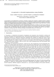
The virtual-lab view is shown in Fig. 4a. The
main window (on the left side of Fig. 4a) contains
the schematic diagram of the process (above)
and the control buttons (below). Both of them
allow the user to experiment with the model.
The user can interactively choose between manual
and automatic control. The automatic control is
intended to perform the following operation policy
(see Fig 4b):
(1) Fill up the reactor with the reacting liquid.
The inflow is controlled by a PID.
(2) Preheat to certain temperature, and let the
reaction proceed adiabatically. The heat exchanger is controlled by another PID.
(3) Start cooling when either the maximum allowable reaction temperature occurs or the
desired conversion is reached, and cool down
to the desired temperature.
(4) Empty the reactor.
The value of the PID-controller parameters, the
temperatures defining the operation policy and
the desired conversion can be changed interactively. Also, the value of the model state-variables
(i.e., the temperature and mass of the reaction
Fig. 4. a) Ejs’ view of the virtual lab; b) Window menu to determine the policy of operation; c) Simulink
model of the virtual lab
mixture, and the concentration of A and P ), the
model parameters (i.e., the reactor volume and
section, the area of the heat exchanger, and the
physicochemical data of the steam and cooling
water), and the input variables (i.e., the inflow
temperature and concentration) can be changed
interactively during the simulation run. The secondary windows on the right side of Fig. 4a contain plots showing the evolution of some relevant
process variables.
5. CONCLUSIONS
A novel modeling methodology adequate for interactive simulation has been proposed. It allows
easy creation of the virtual labs, by combining the
use of Ejs, Matlab/Simulink and Dymola (with
Modelica language). This approach has been successfully applied to the implementation of the
JARA 2i library. The use of Modelica language
has reduced considerably the modeling effort and
it has permitted better reuse of the models. The
use of JARA 2i, Ejs and Matlab/Simulink to develop virtual labs for control education has been
illustrated by means of two case studies.
ACKNOWLEDGEMENTS
Part of this work has been supported by the Spanish CICYT, under DPI2001-1012 and DPI200401804 grants.
REFERENCES
Dormido, S. (2004). Control learning: Present and
future. Annual Reviews in Control 28, 115–
136.
Dynasim (2002). Dymola. User’s Manual. Version
5.0a. Dynasim AB. Lund, Sweden.
Esquembre, F. (2004). Easy Java Simulations: a
software tool to create scientific simulations
in Java. Computer Physics Communications
156, 199–204.
Froment, G.F. and K.B. Bischoff (1979). Chemical
reactor analysis and design. John Wiley &
Sons. New York.
Martin, C., A. Urquia and S. Dormido (2004a).
JARA 2i - A Modelica library for interactive
simulation of physical-chemical processes. In:
Proc. European Simulation and Modelling
Conference. pp. 128–132.
Martin, C., A. Urquia, J. Sanchez, S. Dormido
and F. Esquembre (2004b). Interactive simulation of object-oriented hybrid models, by
combined use of Ejs, Matlab/Simulink and
Modelica/Dymola. In: Proc. 18th European
Simulation Multiconference. pp. 210–215.
Otter, M. and H. Olsson (2002). New features
in Modelica 2.0. In: Proc. 2nd International
Modelica Conference. pp. 7.1–7.12.
Ramirez, W.F. (1989). Computational Methods
for Process Simulation. Butterworths Publishers. Boston.
Urquia, A. (2000). Modelado Orientado a Objetos y Simulación de Sistemas Hı́bridos en el
Ámbito del Control de Procesos Quı́micos.
PhD thesis. Dept. Informática y Automática,
UNED, Madrid, Spain.
Urquia, A. and S. Dormido (2003). Objectoriented design of reusable model libraries of
hybrid dynamic systems. Mathematical and
Computer Modelling of Dynamical Systems
9(1), 65–118.