Download CMG-5T - Guralp Systems Ltd

CMG-5T
Triaxial Accelerometer
Operator's guide
Part No. MAN-050-0001
Designed and manufactured by
Güralp Systems Limited
3 Midas House, Calleva Park
Aldermaston RG7 8EA
England
Proprietary Notice: The information in this manual is
proprietary to Güralp Systems Limited and may not be
copied or distributed outside the approved recipient's
organisation without the approval of Güralp Systems
Limited. Güralp Systems Limited shall not be liable for
technical or editorial errors or omissions made herein,
nor for incidental or consequential damages resulting
from the furnishing, performance, or usage of this
material.
Issue E
2009-12-14
CMG-5T
Table of Contents
1 Introduction...............................................................................................................3
2 Installation.................................................................................................................5
2.1 Unpacking and packing......................................................................................5
2.2 Initial testing.......................................................................................................6
2.3 Installing the sensor...........................................................................................7
2.4 Centring the 5T...................................................................................................8
2.5 Electrical connections........................................................................................9
3 Calibration...............................................................................................................12
3.1 Absolute calibration.........................................................................................12
3.2 Relative calibration...........................................................................................12
3.3 Calibrating accelerometers...............................................................................13
4 Inside the 5T............................................................................................................17
4.1 The force transducer.........................................................................................18
4.2 Frequency response..........................................................................................18
5 Calibration information..........................................................................................21
5.1 Calibration sheet...............................................................................................21
5.2 Poles and zeroes................................................................................................21
6 Connector pinouts...................................................................................................22
6.1 5Ts with high gain output option....................................................................22
6.2 5T high pass filter output option.....................................................................23
7 Specifications..........................................................................................................24
8 Revision history.......................................................................................................25
2
Issue E
Operator's Guide
1 Introduction
The CMG-5T accelerometer is a three-axis strong-motion forcefeedback accelerometer in a sealed case. The sensor system is selfcontained except for its 10 – 36V power supply, which can be
provided through the same cable as the analogue data. An internal
DC–DC converter ensures that the sensor is completely isolated.
The 5T system combines low-noise components with high feedback
loop gain to provide a linear, precision transducer with a very large
dynamic range. In order to exploit the whole dynamic range two
separate outputs are provided, one with high gain and one with low
gain. Nominally, the high gain outputs are set to output a signal 10
times stronger than that from the low gain outputs.
The 5T sensor outputs are all differential with an output impedance of
47 Ω. A single signal ground line is provided as a return line for all the
sensor outputs.
Full-scale low-gain sensitivity is available from 4.0g down to 0.1g. The
most common configuration is for the 5T unit to output 5 V singleended output for 1 g (≈ 9.81 ms-2) input acceleration. The standard
December 2009
3
CMG-5T
frequency pass band is flat to acceleration from DC to 100 Hz
(although other low pass corners from 50 Hz to 100 Hz can be
ordered.) A high frequency option provides flat response from DC to
200 Hz.
Each seismometer is delivered with a detailed calibration sheet
showing its serial number, measured frequency response in both the
long period and the short period sections of the seismic spectrum,
sensor DC calibration levels, and the transfer function in poles/zeros
notation. Installation is simple, using a single fixing bolt to fix the
sensor onto any surface. No sensor levelling is required.
Optionally, you can use a Güralp Control Unit (CU) and Breakout Box
(BB) to distribute power and calibration signals to the sensor and to
receive the signals it produces. The CU can also trim DC offsets during
installation, if required. It is available in both rack-mounted and
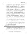
water-resistant portable formats. The accelerometer housing itself is
completely waterproof, with a hard anodised aluminium body and
“O”-ring seals throughout. The photograph below shows two
instruments under test by long-period total immersion in a tank of
water.
4
Issue E
Operator's Guide
2 Installation
2.1 Unpacking and packing
The CMG-5T accelerometer is delivered in a single cardboard box with
foam rubber lining. The packaging is specifically designed for the 5T
and should be reused whenever you need to transport the sensor.
Please note any damage to the packaging when you receive the
equipment, and unpack on a clean surface. The package should
contain:
•
the accelerometer;
•
a signal connection cable (if ordered); and
•
a connector, of type 06F-14-19S.
Place the accelerometer on a clean surface, and identify:
•
The signal cable connector on the top of the unit;
•
The N/S orientation line, engraved on the lid;
•
The N/S orientation pointers (studs);
•
The bubble level;
•
The screw-on cover for the output offset adjuster (see below);
December 2009
5
CMG-5T
•
The central hole for the main fixing bolt; and
•
The serial number. If you need to request the sensor production
history, you will need to quote either the serial number of the
sensor or the works order number, which is also provided on
the calibration sheet.
2.2 Initial testing
To test the 5T before installation, you will need a power source which
can deliver 100 mA at 10 to 36 V and a digital voltmeter (DVM) with 1
and 10 V ranges. Also ensure that the supplied cable is connected with
the correct polarity (see the Appendices).
To make it easier to measure the output from the sensor, you can use a
hand-held Control Unit or a custom interface box, which can be
manufactured from a screw clamp connector block. This will simplify
the connections to the appropriate connector pin outputs.
1. Place the 5T sensor on a flat, horizontal surface.
2. Connect the power supply, observing the correct polarity for
the cable supplied, and switch on.
3. Connect the voltmeter to pins L and M of the output connector
(corresponding to the low gain vertical component.) Measure
the output of the low gain vertical component. The steady
output voltage should be about zero (± 10 mV).
4. Repeat the measurement for the N/S and E/W low-gain
component outputs (pins C/D and K/U respectively).
5. Now gently turn the sensor onto its side, propping it carefully
to prevent rolling.
6. The low gain vertical component should now read about –5 V,
corresponding to –1g.
7. Roll the instrument until the N/S line is vertical, with N at the
top.
8. The low gain N/S component should now read +5 V,
corresponding to +1g.
9. Roll the instrument until the N/S line is horizontal.
10. The low gain E/W component should now read +5 V.
6
Issue E
Operator's Guide
If the performance so far has been as expected, the instrument may be
assumed to be in working order and you may proceed to install the
unit for trial recording tests. Most likely, however, you will need to
adjust the mass deflection offset (see Section 2.4, page 8.)
2.3 Installing the sensor
You will need a solid surface such as a concrete floor to install the 5T.
If you are in any doubt about how to install the sensor, you should
contact Güralp Systems.
1. Prepare the surface by scribing a N/S orientation line, and
installing a grouted-in fixing bolt around the middle of the line.
A 6 mm (0.25 in) threaded stud is suitable, or an expanding-nut
rock bolt or anchor terminating in a threaded stud. The bolt
should be about 120 mm (5 in) long.
2. Place the accelerometer over the stud, on the scribed base-line,
and rotate to bring the orientation line and studs accurately in
alignment with it. The accelerometer has no levelling feet, but
can use an internal simulated level adjustment to compensate as
long as it is fixed to a hard, clean surface within 1 ° of the
horizontal.
3. Fix the accelerometer in place using a fixing nut with spring
washer. Do not over-tighten.
4. If required, make a screening box for the sensor, to shield it
from draughts and sharp changes of temperature. A suitable box
can be constructed from expanded polystyrene slabs (e.g. 5 cm
building insulation slabs) with sealed joints between them and a
hole drilled for the connector. You can then use high-grade glass
fibre sealing tape to fix the leads in position and fasten the box
to the mounting surface. Commercial duct sealing tape is ideal.
5. Connect the sensor to your digitizing equipment or Control Unit
to start receiving signals.
Temporary installations
5T sensors are ideal for monitoring vibrations at field sites, owing to
their ruggedness, high sensitivity and ease of deployment. Temporary
installations will usually be in hand-dug pits or machine-augered
holes. Once a level base is made in the floor, the accelerometer can be
sited there and covered with a box or bucket. One way to produce a
level base is to use a hard-setting liquid:
December 2009
7
CMG-5T
1. Prepare a quick-setting cement/sand mixture, and pour it into
the hole.
2. “Puddle” the cement by vibrating it until it is fully liquefied,
allowing its surface to level out.
3. Depending on the temperature and type of cement used, the
mixture will set over the next 2 to 12 hours.
4. Install the sensor as above, cover, and back-fill the emplacement
with soil, sand, or polystyrene beads.
5. Cover the hole with a turf-capped board to exclude wind noise
and provide a stable thermal environment.
If you prefer, you can use quicker-setting plaster or polyester mixtures
to provide a mounting surface. However, you must take care to prevent
the liquid leaking away by “proofing” the hole beforehand. Dental
plaster, or similar mixtures, may need reinforcing with sacking or
muslin.
Installation in Hazardous environments
The fully enclosed aluminium case design of the 5T instrument makes
it suitable for use in hazardous environments where electrical
discharges due to the build up of static charge could lead to the
ignition of flammable gasses. To ensure safe operation in these
conditions, the metal case of the instrument must be electrically
bonded ('earthed') to the structure on which it is mounted, forming a
path to safely discharge static charge.
Where electrical bonding ('earthing') is required during the installation
of a 5T instrument, the central mounting hole that extends through the
instrument should be used as the connection point. This is electrically
connected to all other parts of the sensor case. Connection can be
made by either a cable from a local earthing point terminated in a
8mm ring tag or via the mounting bolt itself.
2.4 Centring the 5T
Once it is installed, you should centre the instrument ready for use.
The offset can be as much as the entire output range of the
accelerometer, which corresponds to around 1 ° from the horizontal or
vertical. You can check that the 5T is within this range by using the
bubble level on the top of the casing: as long as the bubble lies
completely within the scribed ring, the remaining adjustments can be
made internally.
8
Issue E
Operator's Guide
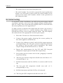
1. Remove the screwed cover protecting the level adjusters. The
cavity contains three adjustment screws, which are arranged as
shown in the diagram below:
2. Power up the sensor, and connect a digital multimeter to its
low-gain vertical outputs (pins L and M). Alternatively, use a
Güralp Systems CMG-5T hand-held control unit to monitor the
outputs more easily.
3. Adjust the vertical screw until the output voltage reads zero.
4. Repeat steps 2 and 3 for the N/S and E/W channels, (pins C/D
and K/U respectively).
5. If necessary, continue to adjust each channel in turn until
consistent results are obtained on all three channels.
6. Repeat steps 2 to 5 using the high-gain outputs, if available, and
refine the settings as far as possible.
7. Replace the protective cover firmly, to keep the instrument's
electronics protected from water and dust.
After the cover is installed, the accelerometer outputs may drift until
the system establishes temperature equilibrium with its environment
and the sensor settles down in its position. If required, the offset
adjustment can be repeated to achieve a better output offset. With
experience, it should be possible to reduce the output level to less than
± 1 mV.
2.5 Electrical connections
Each channel inside the 5T sensor has four output lines: a pair of
December 2009
9
CMG-5T
differential outputs with low gain and another pair with high (around
× 10) gain.
Optionally, the second gain block can be configured at the factory to
act as a high-pass filter to remove the DC offset at the output terminal.
If this is the case, the gain at these outputs will be set to × 1 (unity),
with a separate circuit board providing a filter with a corner frequency
of 0.05 Hz (20 s) or 0.025 Hz (40 s). The output offsets of a high-pass
output cannot be zeroed using the DC offset adjustment screws; in any
case, this offset should not be more than ± 1 mV. The high-pass
output is likely to take around five times the time constant of the highpass circuit to settle down. This time constant is provided on the
calibration sheet, together with accurately-measured frequency values.
The two pairs of output lines are balanced about signal ground so that
either differential drive or single-ended drives of opposite polarity
(phase) are available. For a single-ended drive, the signal ground must
be used as the signal return path. You must not ground any of the
active output lines, as this would allow damaging currents to flow
through the output circuits. Also, if single-ended outputs are used, the
positive acceleration outputs must be interfaced to the recorder.
For distances up to 10 metres, you can connect the sensor outputs
using balanced, screened twin lines terminated with a high-impedance
differential input amplifier. The sensor outputs have a nominal
impedance of 47 Ω.
The 5T is normally powered directly from a connected Güralp digitizer
through the 10-way connector, although you can use a separate
10 – 36 V DC power supply if you wish. The current consumption
from a 12 V supply is about 53 mA. An isolated DC–DC converter
installed inside the sensor housing forms the main part of the 5T unit's
power supply; its filtered outputs provide the ±12 V required to
operate the sensor electronics. The DC–DC converter is protected
against polarity reversal.
The calibration signal and calibration enable inputs are referenced to
the signal ground. If you are using a Güralp digitizer, these lines can
be connected directly to its calibration lines. Otherwise, you will need
to provide a 5 V logic level on the calibration enable input in order to
calibrate the instrument. The signal ground line is used as the return
for both calibration enable and calibration signal lines. See Chapter 3
for more details.
Modifying the sensitivity
This section applies to instruments before serial number T5225 only.
10
Issue E
Operator's Guide
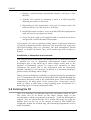
The primary gain block of the 5T is normally set at × 1 (unity). If
higher sensitivity is required, the gain of the instrument can be altered
by inserting gain-setting resistors onto the power supply board of the
unit:
If G is the gain change you require, then the value of the resistors to
insert is given by the formula
R = 10000 / (G – 1)
Care must be taken when soldering these resistors to the circuit board,
as overheating the terminal could easily damage surrounding circuit
elements.
December 2009
11
CMG-5T
3 Calibration
The 5T is supplied with a comprehensive calibration document, and it
should not normally be necessary to calibrate it yourself. However,
you may need to check that the response and output signal levels of
the sensor are consistent with the values given in the calibration
document.
3.1 Absolute calibration
The sensor's response (in V/ms-2) is measured at the production stage
by tilting the sensor through 90 ° and measuring the acceleration due
to gravity. Local g at the Güralp Systems production facility is known
to an accuracy of 5 digits. In addition, sensors are subjected to the
“wagon wheel” test, where they are slowly rotated about a vertical
axis.
The response of the sensor traces out a sinusoid over time, which is
calibrated at the factory to range smoothly from 1g to –1g without
clipping.
3.2 Relative calibration
The response of the sensor, together with several other variables, is
measured at the factory. The values obtained are documented on the
sensor's calibration sheet. Using these, you can convert directly from
voltage (or counts as measured in Scream!) to acceleration values and
back. You can check any of these values by performing calibration
experiments.
Güralp sensors and digitizers are calibrated as described below.
12
Issue E
Operator's Guide
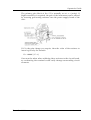
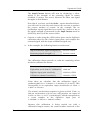
In this diagram a Güralp digitizer is being used to inject a calibration
signal into the sensor. This can be either a sine wave, a step function
or broad-band noise, depending on your requirements. As well as
going to the sensor, the calibration signal is returned to the digitizer on
a full rate channel (older digitizers used one of the 4 Hz auxiliary
(Mux) channels). The calibration signals and sensor output all travel
down the same cable from the sensor to an analogue input port on the
digitizer.
The signal injected into the sensor gives rise to an equivalent
acceleration (EA on the above diagram) which is added to the
measured acceleration to provide the sensor output. Because the
injection circuitry can be a source of noise, a Calibration enable line
from the digitizer is provided which disconnects the calibration circuit
when it is not required. Depending on the factory settings, the
Calibration enable line must be either allowed to float high (+5 to +10
V) or held low (0V, signal ground) during calibration: this is specified
on the sensor's calibration sheet.
The equivalent acceleration corresponding to 1 V of signal at the
calibration input is measured at the factory, and can be found on the
sensor calibration sheet. The calibration sheet for the digitizer
documents the number of counts corresponding to 1 V of signal at
each input port.
The sensor transmits the signal differentially, over two separate lines,
and the digitizer subtracts one from the other to improve the signal-tonoise ratio by increasing common mode rejection. As a result of this,
the sensor output should be halved to give the true acceleration.
CMG-5T instruments are tuned at the factory to produce 1 V of output
for 1 V input on the calibration channel. For example, a sensor with
an acceleration response of 0.25 V/ms-2 should produce 1 V output
given a 1 V calibration signal, corresponding to 1/0.25 = 4 ms-2
= 0.408 g of equivalent acceleration.
3.3 Calibrating accelerometers
Both the DM24 digitizer and Scream! software allow direct
configuration and control of any attached Güralp instruments. For full
information on how to use a DM24 series digitizer, please see its own
documentation. If you are using a third-party digitizer, you can still
calibrate the instrument as long as you activate the Calibration enable
line correctly and supply the correct voltages.
1. In Scream!'s main window, right-click on the digitizer's icon
and select Control.... Open the Calibration pane.
December 2009
13
CMG-5T
2. Select the calibration channel corresponding to the
instrument, make any other choices you require, and click
Inject now. A new data stream, ending Cn (n = 0 – 7) or MB,
should appear in Scream!'s main window containing the
returned calibration signal.
3. Open a Waveview window on the calibration signal and the
returned streams by selecting them and double-clicking. The
streams should display the calibration signal combined with
the sensors' own measurements. If you cannot see the
calibration signal, zoom into the Waveview using the scaling
icons at the top left of the window or the cursor keys.
4. If you need to scale one, but not another, of the traces, rightclick on the trace and select Scale.... You can then type in a
suitable scale factor for that trace.
5. Click on Ampl Cursors in the top right hand corner of the
window. A white square will appear inside the Waveview at
the top left. This is in fact two superimposed cursors.
6. Drag one cursor down to be level with the lowest point of the
signal trace.
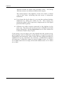
7. Drag the other down to be level with the highest point. In the
following example, a step function of 1 minute duration has
been applied to the Z3 stream. Note that ground movements
continue to be observed, superimposed on the returning
calibration signal.
14
Issue E
Operator's Guide
The Ampl Cursors button will now be displaying a value,
which is the strength of the returning signal in counts
(doubled, if using a sine wave). Measure the other two signal
strengths in this manner.
Note that if you have used the Scale... option described above,
you will need to take the scale factor into account to produce
the correct number of counts. In the example, the MB
(calibration input) signal has been scaled by a factor of 40, so
the signal strength as measured by the Ampl Cursors must be
divided by 40 to yield the correct value.
8. Convert to volts using the µV/Bit values given on the digitizer's
calibration sheet for the various input ports, and compare the
returned signal with the input calibration signal (MB).
9. In the example, the following data are now known:
Input calibration signal strength (MB)
697,221 counts
Returning signal strength (Z3)
701,512 counts
The calibration sheets provide us with the remaining values
needed to calibrate the sensor:
Sensor acceleration response
0.254 V/ms-2
Equivalent accel. from 1V calibration
1.968 ms-2
Digitizer input port sensitivity
3.507212 µV/Bit
Calibration channel sensitivity
3.491621 µV/Bit
From these we calculate that the calibration signal is
producing 697,221 × 3.491621 = 2,434,431 µV (2.434 V). This
corresponds to an equivalent input acceleration of 2.434 ×
1.968 = 4.791 ms-2.
The sensor's acceleration response is given as 0.254 V/ms-2, so
that an acceleration of 4.791 ms-2 will produce an output of
0.254 × 4.791 = 1.217 V (1,216,904 µV), which corresponds to
a count number at the digitizer's input port of
1,216,904 / 3. 507212 = 346,972 counts.
Because this calibration is being carried out with a
differential-output sensor, the count number observed at the
December 2009
15
CMG-5T
digitizer should be double this: 693,944 counts. All Güralp
Systems sensors use balanced differential outputs.
The actual signal at the digitizer of 701,512 counts is within
1.5% of this value, indicating that the sensor is adequately
calibrated.
10. If you know the local value of g, you can also perform absolute
calibration by tilting the sensor by 90 ° and varying the
calibration signal until it precisely compensates for the signal
generated due to gravity.
11. Calibrate any other sensors connected to the digitizer in the
same way. You must wait for the previous calibration to finish
before doing this: clicking Inject now has no effect whilst the
Calibration enable relay is open.
If you prefer, you can inject your own signals into the system at any
point (together with a Calibration enable signal, if required) to provide
independent measurements, and to check that the voltages around the
calibration loop are consistent. For reference, a DM24-series digitizer
will generate a calibration signal of around 16000 counts / 4 V when
set to 100% (sine-wave or step), and around 10000 counts / 2.5 V when
set to 50%.
16
Issue E
Operator's Guide
4 Inside the 5T
The 5T unit is constructed of hard-anodised aluminium with “O” rings
throughout, ensuring a completely waterproof housing.
Inside, the mass of the vertical and horizontal components is attached
to the rigid frame with parallel leaf springs. The geometry of the spring
spacing, together with the symmetrical design, ensures large cross-axis
rejection. The sensor mass is centred between two capacitor plates,
and moves in a true straight line, with no swinging motion. Feedback
coils are attached either side of the sensor mass, forming a constantflux force feedback transducer.
The vertical and horizontal sensors are identical in mechanical
construction; the vertical sensor's mass spring system is adjusted to
compensate for gravity. They are mounted directly onto the base, with
the sensor electronics fixed onto the rigid sensor frame. A single-row,
12-way surface mount R/A Molex connector joins each sensor to the
main power supply circuit board.
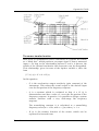
The signal and feedback circuits inside the 5T accelerometer are
arranged according to the following diagram:
December 2009
17
CMG-5T
The mass and the capacitor plates are energised by a two-phase
transformer driver, forming a differential capacitor. This acts as a
capacitive transducer, whose signal is then demodulated with a phasesensitive detector. The accelerometer feedback loop is completed with
a feedback loop compensator and a feedback force transducer power
amp.
The differential output amplifier scales the output sensor sensitivity
and a second stage amplifier can be configured (at the factory) either as
a further cascaded gain stage or as a high-pass filter with unity gain.
4.1 The force transducer
The CMG-5T is a force feedback strong-motion accelerometer which
uses a coil and magnet system to generate the restoring feedback force.
Such accelerometers inherently depend on the production of a
constant-strength field in the magnet gap. Although the high quality
magnets used in the 5T accelerometer are exceedingly stable under
normal conditions, if the sensor is sited in an area where the
background seismic noise is much higher than that of vaults built in
seismically stable locations, the flux density may be affected by the
external magnetic field generated by the feedback transducer coil.
In order to minimise non-linearities in the feedback force transducer,
the 5T uses a symmetrical system of two magnets and two force coils.
Any increase in flux in one coil is cancelled by a corresponding
decrease in flux in the other, thus eliminating any non-linearity due to
lack of symmetry.
4.2 Frequency response
The frequency response of each component is provided as amplitude
and phase plots.
When testing the instrument to confirm that it meets its design
specification, the range of frequencies used are concentrated over
about 3 decades (i.e. 1000 : 1) of excitation frequencies. Consequently,
the frequency plots of each component are provided in normalised
form. Each plot marks the frequency cut-off value (often quoted as “–
3dB” or “half-power” point).
Güralp Systems performs frequency response tests on every sensor at
the time of manufacture. All records are archived for future reference.
18
Issue E
Operator's Guide
The sensor transfer function
Most users of seismometers find it convenient to consider the sensor
as a “black box”, which produces an output signal V from a measured
input x. So long as the relationship between V and x is known, the
details of the internal mechanics and electronics can be disregarded.
This relationship, given in terms of the Laplace variable s, takes the
form
( V / x ) (s) = G × A × H (s)
In this equation
•
G is the acceleration output sensitivity (gain constant) of the
instrument. This relates the actual output to the desired input
over the flat portion of the frequency response.
•
A is a constant which is evaluated so that A × H (s) is
dimensionless and has a value of 1 over the flat portion of the
frequency response. In practice, it is possible to design a system
transfer function with a very wide-range flat frequency
response.
The normalising constant A is calculated at a normalising
frequency value fm = 1 Hz, with s = j fm, where j = √–1.
•
December 2009
H (s) is the transfer function of the sensor, which can be
expressed in factored form:
19
CMG-5T
In this equation zn are the roots of the numerator polynomial, giving the
zeros of the transfer function, and pm are the roots of the denominator
polynomial giving the poles of the transfer function.
In the calibration pack, G is the sensitivity given for each component on
the first page, whilst the roots zn and pm, together with the normalising
factor A, are given in the Poles and Zeros table. The poles and zeros given
are measured directly at Güralp Systems' factory using a spectrum
analyser. Transfer functions for the vertical and horizontal sensors may be
provided separately.
20
Issue E
Operator's Guide
5 Calibration information
Every CMG-5T is supplied with a comprehensive calibration pack
detailing the characteristics of the sensor.
5.1 Calibration sheet
The calibration sheet provides the measured acceleration
responsivities over the flat portion of the sensor frequency response, in
units of volts per metre per second squared (V/ms -2). Because the
sensor produces outputs in differential form (also known as push-pull
or balanced output), the signal received from the instrument by a
recording system with a differential input will be twice the true value.
For example, the calibration sheet may give the acceleration
responsivity as “2 x 0.50 V/ms-2”, indicating that this factor of 2 was
not included in the value given.
Caution: You must never ground any of the differential outputs. If you
are connecting to a single-input recording system, you should use the
signal ground line as the return line.
5.2 Poles and zeroes
The poles and zeroes table describes the frequency response of the
sensor. If required, you can use the poles and zeroes to derive the true
ground motion mathematically from the signal received at the sensor.
The 5T is designed to provide a flat response (to within 3dB) over its
passband. For example, the following curve describes the frequency
response of a 100 Hz sensor:
December 2009
21
CMG-5T
6 Connector pinouts
6.1 5Ts with high gain output option
The 5T sensor has a single connector for both power and signal output.
The following details apply if the second amplification stage is being
used to provide a high (10 ×) gain output channel.
This is a standard 19-pin “mil-spec” plug,
conforming to MIL-DTL-26482 (formerly
MIL-C-26482). A typical part-number is
02E-14-19P although the initial “02E” varies
with manufacturer.
Suitable mating connectors have partnumbers like ***-14-19S and are available
from Amphenol, ITT Cannon and other
manufacturers.
Pin Function
Pin Function
A
High gain +ve, N/S channel
L
Low gain –ve, vertical channel
B
High gain –ve, N/S channel
M Low gain +ve, vertical channel
C
Low gain +ve, N/S channel
N
High gain –ve, vertical channel
D
Low gain –ve, N/S channel
P
High gain +ve, vertical channel
E
Calibration signal (all channels)
R
High gain +ve, E/W channel
F
Power +12 V (all channels)
S
Calibration enable (all channels)
G
Power 0 V (all channels)
T
Signal ground (essential if a long
power cable is used)
H
not connected
U
Low gain +ve, E/W channel
J
Open/closed loop (all channels)
V
High gain –ve, E/W channel
K
Low gain –ve, E/W channel
Wiring details for the compatible socket,
***-14-19S, as seen from the cable end.
22
Issue E
Operator's Guide
6.2 5T high pass filter output option
The following table applies if the second amplification stage is being
used to provide a high-pass filter (with unity gain). The same
connector is used and the connector information above (in Section 6.1)
applies.
Pin Function
A
High pass filtered acceleration +ve, N/S channel
B
High pass filtered acceleration –ve, N/S channel
C
Acceleration +ve, N/S channel
D
Acceleration –ve, N/S channel
E
Calibration signal (all channels)
F
Power +12 V (all channels)
G
Power 0 V (all channels)
H
Power –12 V (all channels)
J
Open/closed loop (all channels)
K
Acceleration –ve, E/W channel
L
Acceleration –ve, vertical channel
M
Acceleration +ve, vertical channel
N
High pass filtered acceleration –ve, vertical channel
P
High pass filtered acceleration +ve, vertical channel
R
High pass filtered acceleration +ve, E/W channel
S
Calibration enable (all channels)
T
Signal ground (essential if a long power cable is used)
U
Acceleration +ve, E/W channel
V
High pass filtered acceleration –ve, E/W channel
December 2009
23
CMG-5T
7 Specifications
Outputs and
response
Calibration
controls
Physical
Power
24
Low gain output options
2g, 1g, 0.5g, 0.1g
Corresponding high gain
outputs
0.2g, 0.1g, 0.05g, 0.01g
Dynamic range at 2 g
standard
Dynamic range, 0.005 –
0.05 Hz
< 140 dB
Dynamic range, 3 – 30 Hz
< 127 dB
Standard frequency band
DC – 100 Hz (–3dB
point)
Optional low-pass corner
50, 100 or 200 Hz
Linearity
0.1 % of full scale
Cross-axis rejection
0.001g / g
Open-loop response
pin on connector
Closed-loop response
pin on connector
Step function response
may be added to openand closed-loop
calibrations
External inputs
Sine-wave, step, or
pseudo-random
Lowest spurious resonance 450 Hz
Operating temperature
range
–20° to +70 °C
Pressure jacket material
hard anodised
aluminium
Power / signal connector
Mil-spec connector on
sensor housing (02E14-19P)
Weight
2,270 g
Current at 12 V DC
8 mA per axis
Issue E
Operator's Guide
8 Revision history
1009-12-14 E
Revised calibration section and new “internals”
diagram.
2009-10-05 D
Additional connector information and some purely
cosmetic changes
2007-11-20 C
added.
Installation in hazardous environments section
2006-09-22 B
Added revision history
2006-01-06 A
New document
December 2009
25