Download Control Flow Graphs for Real-Time System Analysis

Control Flow Graphs for Real-Time System Analysis
Reconstruction from Binary Executables
and
Usage in ILP-Based Path Analysis
Dissertation
Zur Erlangung des Grades
Doktor der Ingenieurwissenschaften
(Dr.-Ing.)
der Naturwissenschaftlich-Technischen Fakultät I
der Universität des Saarlandes
von
Diplominformatiker
Henrik Theiling
aus Saarbrücken
Saarbrücken 2002
Tag des Kolloquiums:
4. Februar 2003
Dekan:
Prof. Dr.-Ing. Philipp Slusallek
Vorsitzender:
Prof. Dr.-Ing. Gerhard Weikum
Gutachter:
als Vertretung im Kolloquium:
Prof. Dr. Reinhard Wilhelm
Prof. Dr. Harald Ganzinger
Prof. Dr. Andreas Podelski
Beisitzer:
Dr.-Ing. Ralf Schenkel
Abstract
Real-time systems have to complete their actions w.r.t. given timing constraints. In order to validate that these constraints are
met, static timing analysis is usually performed to compute an
upper bound of the worst-case execution times (WCET) of all the
involved tasks.
This thesis identifies the requirements of real-time system analysis on the control flow graph that the static analyses work on.
A novel approach is presented that extracts a control flow graph
from binary executables, which are typically used when performing WCET analysis of real-time systems.
Timing analysis can be split into two steps: a) the analysis of the
behaviour of the hardware components, b) finding the worst-case
path. A novel approach to path analysis is described in this thesis that introduces sophisticated interprocedural analysis techniques that were not available before.
3
4
Zusammenfassung
Echtzeitsysteme müssen ihre Aufgaben innerhalb vorgegebener
Zeitschranken abwickeln. Um die Einhaltung der Zeitschranken
zu überprüfen, sind für gewöhnlich statische Analysen der
schlimmsten Ausführzeiten der Teilprogramme des Echtzeitsystems nötig.
Diese Arbeit stellt die Anforderungen von Echtzeitsystem an
den Kontrollflußgraphen vor, auf dem die statischen Analysen arbeiten. Ein neuartiger Ansatz zur Rückberechnung von Kontrollflußgraphen aus Maschinenprogrammen, die häufig die
Grundlage der WCET-Analyse von Echtzeitsystemen bilden,
wird vorgestellt.
WCET-Analysen können in zwei Teile zerlegt werden: a) die
Analyse des Verhaltens der Hardwarebausteine, b) die Suche
nach dem schlimmsten Ausführpfad. In dieser Arbeit wird ein
neuartiger Ansatz der Pfadanalyse vorgestellt, der für ausgefeilte
interprozedurale Analysemethoden ausgelegt ist, die vorher hier
nicht verfügbar waren.
5
6
Extended Abstract
Real-time systems are computer systems that have to perform their actions with fulfilment of timing constraints. Additional to performing the actions correctly, their correctness also depends on the fulfilments of these timing constraints.
The validation of timing aspects is called a schedulability analysis. A real-time system
often consists of many tasks. Existing techniques for schedulability analysis require
that the worst-case execution time (WCET) of each task is known.
Since the real WCET of a program is in general not computable, an upper bound to the
real WCET has to be computed instead. For real-time systems, these WCET predictions
must be safe, i. e., the real WCET must never be underestimated. On the other hand, to
increase the probability of a successful schedulability analysis, the predictions should
be as precise as possible.
Most static analyses, including approaches to WCET analysis, examine the control flow
of the program. Because the behaviour of the program is typically not known in advance, an approximation to the control flow is used as the basis of the analysis. This
approximation is called a control flow graph.
For good performance, modern real-time systems use modern hardware architectures.
These use heuristic components, like caches and pipelines, to speed up the program in
typical situations. Neglecting these speed up factors in a WCET analysis would lead to
a dramatic overestimation of the real WCET of the program.
For taking into account hardware components, the program usually has to be analysed
at the hardware level. Therefore, binary executables are the bases of analyses. Further, the
timing behaviour of typical modern hardware depends on the data that is processed,
and in particular on the addresses that are used to access memory. Again, full information about addresses is available from binary executables.
7
The first part of this work presents a novel approach to extracting control flow graphs
from binary executables. The general task is non-trivial, since often, the possible control
flow is not obvious, e. g., when function pointers, switch tables or dynamic dispatch
come into play. Further, it is often hard to predict what is the influence of a certain
machine instruction on control flow, e. g., because its usage is ambiguous.
The reconstruction algorithms presented in this work are designed with real-time systems in mind. The requirements for a safe analysis also have to be considered during
the extraction of control flow graphs from binaries, since analyses can only be safe if the
underlying data structure is safe, too.
The reconstruction of control flow graphs from binary executables will be conceptually
split into two separate tasks: a) given a stream of bytes from a binary executable and
the address in the processor’s code pointer, the precise classification of the instruction
that will be executed by the machine, b) given a set of instruction classifications and
possible program start nodes, the automatic composition of a safe and precise control
flow graph.
For solving the first task, we will use very efficient decision trees to convert raw bytes into
instruction classifications. An algorithm will be presented that computes the decision
trees automatically from very concise specifications that can trivially be derived from
the vendor’s architecture documentation. This is a novel approach that extricates the
user from error-prone programming that had to be done in the past.
For the reconstruction of control flow from a set of instruction classifications, a bottomup approach will be presented. This algorithm overcomes problems that top-down approaches usually have. Top-down approaches are fine for producing disassembly listings and for debugging purposes, but static analysis poses additional requirements on
safety and precision that top-down algorithms cannot fulfil. Our bottom-up approach
meets these requirements. Furthermore, it is implemented very efficiently.
The second part of this work deals with the analysis of real-time systems itself. Timing
analysis that is close to hardware can be split into two parts: a) the analysis of the
behaviour of the components at all blocks of the program and b) the computation of a
global upper bound for the WCET based on the results of the analysis of each block.
The latter analysis is called the path analysis.
An established technique of path analysis uses Integer Linear Programming (ILP). The
idea is as follows: the program’s control flow is described by a set of constraints, and the
execution times of the program’s blocks are combined in an objective function. The task
of finding an upper bound of the WCET of the whole program is solved by maximising
the objective function under consideration of the control flow constraints.
Because of the complex behaviour of modern hardware, sophisticated techniques for
WCET analysis must typically be used. For instance, routine invocations in the program should not be analysed in isolation, since their timing behaviour may be very
8
different from invocation to invocation. This is because the state of the machine’s hardware components is typically very different for each invocation and this state influences
performance a lot.
For this reason, analyses usually perform better when they consider routine invocations
in different execution contexts, where the contexts depend on the history of the program
execution.
To make use of contexts, both parts of WCET analysis, the analysis of the hardware
components and the path analysis must handle them. Up to now, it was not examined
how path analysis can be done with arbitrary static assignment of execution contexts.
This work will close this gap by presenting a new approach to ILP-based path analysis
that can handle contexts, providing a high degree of flexibility to the user of the WCET
analysis tool.
All algorithms presented in this thesis are implemented in tools that are now widely
used in educational as well as industrial applications.
9
10
Ausführliche Zusammenfassung
Echtzeitsysteme sind Computersysteme, die ihre Aufgaben innerhalb vorgegebener
Zeitschranken erfüllen müssen. Zu ihre Korrektheit gehört zusätzlich zur funktionalen
Korrektheit die Einhaltung dieser Zeitschranken.
Die Überprüfung des korrekten Zeitverhaltens nennt man Planbarkeitsanalyse (engl.:
schedulability analysis). Ein Echtzeitsystem besteht häufig aus mehreren Teilprogrammen. In allen bekannten Ansätzen zur Planbarkeitsanalyse wird vorrausgesetzt, daß
die schlimmste Ausführzeit (WCET, von engl. worst-case execution time) jedes einzelnen
Teilprogramms bekannt ist.
Da die wirkliche Maximallaufzeit eines Programmes im allgemeinen nicht berechenbar ist, wird stattdessen eine obere Schranke berechnet. Bei Echtzeitsystemen müssen
diese Vorhersagen sicher sein, d. h. die wirkliche Maximallaufzeit des Programmes darf
niemals unterschätzt werden. Weiterhin sollten die Vorhersagen möglichst genau sein,
um die Wahrscheinlichkeit einer erfolgreichen Planbarkeitsanalyse zu erhöhen.
Die meisten statischen Analysen, die WCET-Analyse eingeschlossen, untersuchen den
Kontrollfluß eines Programmes. Da aber das Verhalten normalerweise vor Ablauf des
Programms nicht bekannt ist, müssen Analysen mit einer Annäherung an den Kontrollfluß vorliebnehmen. Diese Annäherung nennt man Kontrollflußgraph.
Heutige Echtzeitsystem benutzen moderne Hardware, um deren Leistungsvorteile
auszunutzen. Die Architekturen benutzen häufig heuristische Bausteine, wie Caches
oder Pipelines, die die Ausführungsgeschwindigkeit des Programmes in häufig vorkommenden Situationen erhöhen sollen. Um starke Überschätzungen der Laufzeit zu
vermeiden, muß eine WCET-Analyse typischerweise das Verhalten dieser Bausteine
mitberücksichtigen.
Zur Vorhersage des Verhaltens von Hardwarebausteinen ist es normalerweise erforder11
lich, das Programm hardwarenah zu analysieren. Daher benutzt man für die Analyse
das Maschinenprogramm. Die Ausführgeschwindigkeit hängt auch von den verarbeiteten Daten ab, vor allem von den Adressen, die zum Zugriff auf den Speicher benutzt werden. Auch aus diesem Grund verwendet man Maschinenprogramme, denn
die nötigen Informationen sind dort vorhanden.
Im ersten Teil dieser Arbeit wird ein neuartiger Ansatz zur Rückberechnung von
Kontrollflußgraphen aus Maschinenprogrammen vorgestellt. Die allgemeine Aufgabe
ist schwierig, denn oft ist der mögliche Kontrollfluß nicht offensichtlich, z. B. bei
der Verwendung von Funktionszeigern, switch-Tabellen oder dynamischen Methodenaufrufen. Desweiteren ist es häufig schwierig, vorherzusagen, welchen Einfluß bestimmte Befehlen auf den Kontrollfluß haben, da diese mitunter in verschiedenen Situationen auftauchen.
Der in dieser Arbeit vorgestellte Algorithmus zur Rückberechnung von Kontrollflußgraphen wurde unter besonderer Beachtung der speziellen Anforderungen von
Echtzeitsystemanalyse entwickelt, denn ohne eine sichere Rückberechnung von Kontrollflußgraphen können darauf arbeitende Analysen ebenfalls nicht sicher sein.
Die Rückberechnung läßt sich in zwei Phasen zerlegen: a) die Erstellung einer Klassifizierung eines Maschinenbefehls bei Eingabe eines Byte-Stroms und der Adresse des
Befehls, b) die automatische Rückberechnung eines sicheren und genauen Kontrollflußgraphen bei Eingabe einer Menge von Befehlsklassifikationen.
Um die erste Aufgabe zu lösen, werde ich einen sehr effizienten Entscheidungsbaum
vorstellen, mit dessen Hilfe sich eine Folge roher Bytes in eine Befehlsklassifikation umwandeln läßt. Ein Algorithmus zur automatischen Berechnung eines solchen
Entscheidungsbaums wird vorgestellt werden, der als Eingabe einzig eine Spezifikation erhält, die sich leicht aus der Architekturbeschreibung des Herstellers erstellen läßt.
Dieser Ansatz befreit den Benutzer von fehlerträchtiger Programmierarbeit, die bisher
nötig war.
Zur Rückberechnung eines Kontrollflußgraphen aus einer Menge von Befehlsklassifikationen wird ein Bottom-Up-Ansatz vorgestellt werden. Dieser überwindet Probleme von
Top-Down-Ansätzen, die sich zwar gut zum Programmieren von Disassemblern oder
Debuggern eignen, aber keineswegs den Anforderungen von Echtzeitsystemen gerecht
werden. Unser Bottom-Up-Ansatz hingegen wird diesen gerecht und ist zudem sehr
effizient implementiert.
Der zweite Teil dieser Arbeit behandelt die Analyse von Echtzeitsystemen selbst. Hardwarenahe WCET-Analyse kann man in zwei Teile aufspalten: a) die Analyse des Verhaltens der Hardwarebausteine für jeden Block des Programmes, b) die Berechnung einer
oberen Schranke der WCET des Programms basierend auf den Ergebnissen der Analyse
in a). b) nennt man Pfadanalyse.
Eine verbreitete Methode der Pfadanalyse benutzt Ganzzahlige Lineare Program12
mierung (ILP von engl. Integer Linear Programming). Die Idee dabei ist, daß man den
Kontrollfluß des Programmes durch Nebenbedingungen beschreibt und die Laufzeiten
der einzelnen Blöcke des Programmes in einer Zielfunktion zusammenfaßt. Das Maximierungsproblem der Zielfunktion unter Beachtung der Nebenbedingungen löst dann
das Problem der Suche nach einer oberen Schranke für die Maximallaufzeit des Programmes.
Weil moderne Hardware sich komplex verhält, müssen normalerweise ausgefeilte
Methoden zur WCET-Analyse verwendet werden. Beispielsweise sollten Routinenaufrufe nicht isoliert behandelt werden, da sich ihr Verhalten von Aufruf zu Aufruf
stark unterscheiden kann. Das liegt daran, daß der Zustand der Hardwarebausteine die
Ausführzeiten stark beeinflussen.
Aus diesem Grunde verbessert man die Vorhersagen für gewöhnlich, indem man Routinenaufrufe in verschiedenen Kontexten analysiert, wobei die Kontexte davon abhängen,
was im Programm vorher schon ausgeführt wurde.
Um von Kontexten Gebrauch zu machen, müssen beide Teile der WCET-Analyse, die
der Bausteine und die Pfadanalyse, sie verarbeiten können. Bisher war es nicht untersucht, wie man auf ILP beruhende Pfadanalysen mit beliebigen statisch berechneten
Kontextzuweisungen durchführen kann. Diese Arbeit schließt diese Lücke und stellt
einen Ansatz vor, der dem Benutzer des Analysewerkzeugs einen hohen Grad an Freiheit überläßt.
Alle in dieser Arbeit vorgestellten Algorithmen sind in Werkzeugen implementiert, die
inzwischen in universitärem wie industriellem Gebrauch sind.
13
14
Acknowledgements
First of all, I very much thank Reinhard Wilhelm for letting me have the opportunity
to work and research at his chair and to write my thesis about this challenging and
interesting topic. He was very helpful in discussions about this work and provided me
with a lot of freedom for approaching my goals.
The research group provided a very pleasant working atmosphere. I would like to thank
Michael Schmidt for our good team work with discussions about interfaces, implementation and algorithms. We implemented parts of the overall WCET framework together
and Michael also contributed by writing some modules for exec2crl. Thanks are also
due to Florian Martin and Christian Ferdinand for fruitfully discussing a lot of different
topics with me. They often found peculiarities and had many hints and ideas. Thanks
to Reinhold Heckmann for providing helpful thoughts and links to other peoples’ research from most different areas of computer science. He was also a great help for me
by proof-reading this thesis.
For excellent team work and discussions, I also thank Daniel Kästner, Marc Langenbach
and Martin Sicks. Nico Fritz did a magnificent job implementing the ARM decoder
module for exec2crl, despite his being a complete novice to its internal structure when
he began.
During international conferences and other occasions, the whole real-time community
constituted a nice atmosphere. Most notably, I had a lot of discussions with Sheayun
Lee, Sungsoo Lim, Jan Gustafsson, Jakob Engblom and Andreas Ermedahl.
Thanks to Uta Hengst, Björn Huke, Daniel Kästner, Markus Löckelt and Nicola Wolpert
for proof-reading parts of this work and giving valuable hints.
Last but not least, I would like to thank my family for their support during the time of
my research and also Uta Hengst and Florian Martin for continuously reminding me to
work hard.
15
16
Contents
I Introduction
23
1 Introduction
25
1.1
Timing Analysis of Real-Time Systems . . . . . . . . . . . . . . . . . . . . . 25
1.2
Control Flow Graphs . . . . . . . . . . . . . . . . . . . . . . . . . . . . . . . 27
1.3
Path Analysis . . . . . . . . . . . . . . . . . . . . . . . . . . . . . . . . . . . 28
1.4
Scope of this Thesis . . . . . . . . . . . . . . . . . . . . . . . . . . . . . . . . 30
2 Basics
33
2.1
Selected Mathematical Notations . . . . . . . . . . . . . . . . . . . . . . . . 33
2.2
Program Structure . . . . . . . . . . . . . . . . . . . . . . . . . . . . . . . . . 34
2.2.1
Programs and Instructions
. . . . . . . . . . . . . . . . . . . . . . . 34
2.2.2
Basic Blocks . . . . . . . . . . . . . . . . . . . . . . . . . . . . . . . . 35
2.2.3
Routines . . . . . . . . . . . . . . . . . . . . . . . . . . . . . . . . . . 35
2.2.4
Control Flow Graph . . . . . . . . . . . . . . . . . . . . . . . . . . . 36
2.2.5
Call Graph . . . . . . . . . . . . . . . . . . . . . . . . . . . . . . . . . 36
2.2.6
Example in C . . . . . . . . . . . . . . . . . . . . . . . . . . . . . . . 37
2.2.7
Loops . . . . . . . . . . . . . . . . . . . . . . . . . . . . . . . . . . . . 38
17
Contents
2.3
Integer Linear Programming . . . . . . . . . . . . . . . . . . . . . . . . . . . 41
2.3.1
Linear Programs . . . . . . . . . . . . . . . . . . . . . . . . . . . . . 41
2.3.2
Simplex Algorithm . . . . . . . . . . . . . . . . . . . . . . . . . . . . 43
2.3.3
Integer Linear Programs . . . . . . . . . . . . . . . . . . . . . . . . . 44
2.3.4
Branch and Bound Algorithm . . . . . . . . . . . . . . . . . . . . . . 45
3 Control Flow Graphs
3.1
3.2
3.3
47
Control Flow Graphs for Real-Time System Analysis . . . . . . . . . . . . . 47
3.1.1
Safety . . . . . . . . . . . . . . . . . . . . . . . . . . . . . . . . . . . . 47
3.1.2
Precision . . . . . . . . . . . . . . . . . . . . . . . . . . . . . . . . . . 48
Detailed Structure of CFG and CG . . . . . . . . . . . . . . . . . . . . . . . . 48
3.2.1
Alternative Control Flow and Edge Types . . . . . . . . . . . . . . . 49
3.2.2
Unrevealed Control Flow . . . . . . . . . . . . . . . . . . . . . . . . 50
3.2.3
Calls . . . . . . . . . . . . . . . . . . . . . . . . . . . . . . . . . . . . 50
3.2.4
External Routines . . . . . . . . . . . . . . . . . . . . . . . . . . . . . 52
3.2.5
Difficult Control Flow . . . . . . . . . . . . . . . . . . . . . . . . . . 53
Contexts . . . . . . . . . . . . . . . . . . . . . . . . . . . . . . . . . . . . . . 54
3.3.1
CallString k
3.3.2
Graphs with Context . . . . . . . . . . . . . . . . . . . . . . . . . . . 57
3.3.3
Iteration Counts for Contexts . . . . . . . . . . . . . . . . . . . . . . 59
3.3.4
Recursive Example . . . . . . . . . . . . . . . . . . . . . . . . . . . . 59
3.3.5
VIVU
3.3.6
Example . . . . . . . . . . . . . . . . . . . . . . . . . . . . . . . . . . 63
. . . . . . . . . . . . . . . . . . . . . . . . . . . . . . . . 56
n k . . . . . . . . . . . . . . . . . . . . . . . . . . . . . . . . . . 60
II Control Flow Graphs and Binary Executables
65
4 Introduction
67
18
4.1
Problems . . . . . . . . . . . . . . . . . . . . . . . . . . . . . . . . . . . . . . 69
4.2
Steps of Control Flow Reconstruction . . . . . . . . . . . . . . . . . . . . . 70
Contents
4.3
Versatility . . . . . . . . . . . . . . . . . . . . . . . . . . . . . . . . . . . . . 71
5 Machine Code Decoding
5.1
5.2
5.3
5.4
5.5
Introduction . . . . . . . . . . . . . . . . . . . . . . . . . . . . . . . . . . . . 73
5.1.1
Bit Patterns . . . . . . . . . . . . . . . . . . . . . . . . . . . . . . . . 73
5.1.2
Selected Design Goals . . . . . . . . . . . . . . . . . . . . . . . . . . 74
5.1.3
Chapter Overview . . . . . . . . . . . . . . . . . . . . . . . . . . . . 76
Data Structure . . . . . . . . . . . . . . . . . . . . . . . . . . . . . . . . . . . 76
5.2.1
Selection Algorithm . . . . . . . . . . . . . . . . . . . . . . . . . . . 77
5.2.2
Restrictions on Pattern Sets . . . . . . . . . . . . . . . . . . . . . . . 79
Automatic Tree Generation . . . . . . . . . . . . . . . . . . . . . . . . . . . 80
5.3.1
Idea . . . . . . . . . . . . . . . . . . . . . . . . . . . . . . . . . . . . . 80
5.3.2
Algorithm . . . . . . . . . . . . . . . . . . . . . . . . . . . . . . . . . 81
5.3.3
Default Nodes . . . . . . . . . . . . . . . . . . . . . . . . . . . . . . . 83
5.3.4
Unresolved Bit Patterns . . . . . . . . . . . . . . . . . . . . . . . . . 85
5.3.5
Termination . . . . . . . . . . . . . . . . . . . . . . . . . . . . . . . . 85
5.3.6
Proof of Correctness . . . . . . . . . . . . . . . . . . . . . . . . . . . 85
Efficient Implementation . . . . . . . . . . . . . . . . . . . . . . . . . . . . . 87
5.4.1
Complexity . . . . . . . . . . . . . . . . . . . . . . . . . . . . . . . . 88
5.4.2
Generalisation . . . . . . . . . . . . . . . . . . . . . . . . . . . . . . . 88
Summary . . . . . . . . . . . . . . . . . . . . . . . . . . . . . . . . . . . . . . 88
6 Reconstruction of Control Flow
6.1
89
Introduction . . . . . . . . . . . . . . . . . . . . . . . . . . . . . . . . . . . . 89
6.1.1
6.2
73
Overview . . . . . . . . . . . . . . . . . . . . . . . . . . . . . . . . . 90
Approaches to Control Flow Reconstruction
. . . . . . . . . . . . . . . . . 90
6.2.1
Top-Down Approach . . . . . . . . . . . . . . . . . . . . . . . . . . . 91
6.2.2
Problems Unsolved by Top-Down Approach . . . . . . . . . . . . . 92
6.2.3
Intuition of Bottom-Up Approach . . . . . . . . . . . . . . . . . . . 94
19
Contents
6.2.4
Theory . . . . . . . . . . . . . . . . . . . . . . . . . . . . . . . . . . . 95
6.3
Modular Implementation . . . . . . . . . . . . . . . . . . . . . . . . . . . . 97
6.4
The Core Algorithms . . . . . . . . . . . . . . . . . . . . . . . . . . . . . . . 99
6.5
6.4.1
Gathering Routines . . . . . . . . . . . . . . . . . . . . . . . . . . . . 99
6.4.2
Decoding a Routine . . . . . . . . . . . . . . . . . . . . . . . . . . . 99
6.4.3
Properties of the Algorithm . . . . . . . . . . . . . . . . . . . . . . . 101
Implementation . . . . . . . . . . . . . . . . . . . . . . . . . . . . . . . . . . 103
6.5.1
PowerPC . . . . . . . . . . . . . . . . . . . . . . . . . . . . . . . . . . 104
6.5.2
Infineon TriCore . . . . . . . . . . . . . . . . . . . . . . . . . . . . . 105
6.5.3
ARM . . . . . . . . . . . . . . . . . . . . . . . . . . . . . . . . . . . . 105
III Path Analysis
107
7 Implicit Path Enumeration (IPE)
109
7.1
Times and Execution Counts . . . . . . . . . . . . . . . . . . . . . . . . . . . 109
7.2
Handling Special Control Flow . . . . . . . . . . . . . . . . . . . . . . . . . 110
7.3
7.2.1
External Routine Invocations . . . . . . . . . . . . . . . . . . . . . . 110
7.2.2
Unresolved Computed Branches . . . . . . . . . . . . . . . . . . . . 111
7.2.3
Unresolved Computed Calls . . . . . . . . . . . . . . . . . . . . . . 111
7.2.4
No-return calls . . . . . . . . . . . . . . . . . . . . . . . . . . . . . . 111
ILP . . . . . . . . . . . . . . . . . . . . . . . . . . . . . . . . . . . . . . . . . 112
7.3.1
Objective Function . . . . . . . . . . . . . . . . . . . . . . . . . . . . 112
7.3.2
Program Start Constraint . . . . . . . . . . . . . . . . . . . . . . . . 113
7.3.3
Structural Constraints . . . . . . . . . . . . . . . . . . . . . . . . . . 113
7.3.4
Loop Constraints . . . . . . . . . . . . . . . . . . . . . . . . . . . . . 115
7.3.5
Time Bounded Execution . . . . . . . . . . . . . . . . . . . . . . . . 116
7.3.6
User Added Constraints . . . . . . . . . . . . . . . . . . . . . . . . . 117
8 Interprocedural Path Analysis
20
119
Contents
8.1
8.2
8.3
Basic Constraints . . . . . . . . . . . . . . . . . . . . . . . . . . . . . . . . . 119
8.1.1
Objective Function . . . . . . . . . . . . . . . . . . . . . . . . . . . . 120
8.1.2
Program Start Constraint . . . . . . . . . . . . . . . . . . . . . . . . 120
8.1.3
Structural Constraints . . . . . . . . . . . . . . . . . . . . . . . . . . 120
Loop Bound Constraints . . . . . . . . . . . . . . . . . . . . . . . . . . . . . 121
8.2.1
Simple Loop Bound Constraints . . . . . . . . . . . . . . . . . . . . 122
8.2.2
Loop Bound Constraints for VIVU x ∞
8.2.3
Loop Bound Constraints for Arbitrary Mappings . . . . . . . . . . 127
. . . . . . . . . . . . . . . . 125
User Added Constraints . . . . . . . . . . . . . . . . . . . . . . . . . . . . . 134
IV Evaluation
135
9 Experimental Results
137
9.1
Implementation . . . . . . . . . . . . . . . . . . . . . . . . . . . . . . . . . . 137
9.2
Decision Trees . . . . . . . . . . . . . . . . . . . . . . . . . . . . . . . . . . . 137
9.3
CFG Reconstruction . . . . . . . . . . . . . . . . . . . . . . . . . . . . . . . . 139
9.4
Path Analysis . . . . . . . . . . . . . . . . . . . . . . . . . . . . . . . . . . . 141
10 Related Work
147
10.1 History of WCET Analysis . . . . . . . . . . . . . . . . . . . . . . . . . . . . 147
10.1.1 Abstract Interpretation . . . . . . . . . . . . . . . . . . . . . . . . . . 147
10.1.2 Worst-Case Execution Time Analysis . . . . . . . . . . . . . . . . . . 148
10.2 Decision Trees . . . . . . . . . . . . . . . . . . . . . . . . . . . . . . . . . . . 150
10.3 ICFG Reconstruction . . . . . . . . . . . . . . . . . . . . . . . . . . . . . . . 151
10.4 Path Analysis . . . . . . . . . . . . . . . . . . . . . . . . . . . . . . . . . . . 152
11 Conclusion
155
11.1 Decision Trees . . . . . . . . . . . . . . . . . . . . . . . . . . . . . . . . . . . 155
11.2 CFG Reconstruction . . . . . . . . . . . . . . . . . . . . . . . . . . . . . . . . 156
21
Contents
11.3 Path Analysis . . . . . . . . . . . . . . . . . . . . . . . . . . . . . . . . . . . 157
11.4 History & Development . . . . . . . . . . . . . . . . . . . . . . . . . . . . . 157
11.5 Outlook . . . . . . . . . . . . . . . . . . . . . . . . . . . . . . . . . . . . . . . 158
11.5.1 Cycles . . . . . . . . . . . . . . . . . . . . . . . . . . . . . . . . . . . 158
11.5.2 CFG Reconstruction . . . . . . . . . . . . . . . . . . . . . . . . . . . 159
11.5.3 Architectures . . . . . . . . . . . . . . . . . . . . . . . . . . . . . . . 159
A Experiments in Tables and Figures
161
A.1 Path Analysis . . . . . . . . . . . . . . . . . . . . . . . . . . . . . . . . . . . 161
A.1.1 One Loop, One Invocation . . . . . . . . . . . . . . . . . . . . . . . . 161
A.1.2 One Loop, Two Invocations . . . . . . . . . . . . . . . . . . . . . . . 164
A.1.3 Two Loops . . . . . . . . . . . . . . . . . . . . . . . . . . . . . . . . . 166
A.1.4 Recursion with Two Loop Entries . . . . . . . . . . . . . . . . . . . 169
22
Part I
Introduction
Chapter 1
Introduction
1.1 Timing Analysis of Real-Time Systems
The fundamental characteristic of real-time systems is that they are subject to timing
constraints that determine when actions have to be taken. The fulfilment of these timing
constraints, additional to the operational results, is part of the correctness of a real-time
system.
In literature, real-time systems are usually divided into two types: hard and soft realtime systems, depending on whether their timing constraints are imperative or desirable. If not explicitly stated otherwise, the term real-time system will be used for a hard
real-time system in this work. The imperative nature of the timing constraints makes
static analysis particularly interesting for real-time system validation.
Real-time systems occur in many areas, e. g. in process control, nuclear power plants,
avionics, air traffic control, medical devices, defence applications and controllers in automobiles.
A failure of a safety critical real-time system can lead to considerable damage or even a
loss of lives. Therefore, the system must be validated. Among other properties, it has
to be shown that it fulfils all its timing constraints. The validation of timing aspects is
called a schedulability analysis (see [Liu and Layland., 1973; Stankovic, 1996]).
A real-time system is often composed of many tasks. All existing techniques for schedulability analysis require the worst-case execution time (WCET) of each task in the system
25
Chapter 1. Introduction
to be known.
Since the exact WCET is in general not computable, estimations of the WCET have to be
calculated. These estimations have to be safe, meaning they must never underestimate
the actual WCET.
On the other hand, the WCET approximation should be tight, i. e., the overestimation
should be as small as possible. This helps to reduce the costs for the hardware and
increases the chances of a successful timing validation.
For simple hardware, i. e. for a processor with a fixed execution time for each instruction, estimation of the WCET is quite easy: if each instruction’s execution time is known,
the WCET can be computed by recursively combining execution times along the syntax
tree of the program. This method was used in [Puschner and Koza, 1989] and in [Park
and Shaw, 1991].
Modern hardware, however, becomes increasingly difficult to predict due to sophisticated heuristic components that increase execution speed of instructions for common
special cases, which most likely make programs much faster on average, while single
instructions may still be slow. This means that simple, conservative analysis techniques
strongly overestimate the actual WCET.
The execution time of an instruction may depend on the internal state of the processor.
This state gets more and more complex with the presence of the mentioned heuristic
components. Therefore, predicting the relevant parts of the processor’s internal state
that influence the timing behaviour becomes more and more difficult. The following
list shows some components of modern hardware that make predictions complicated.
Pipelines. Processing of a single instruction is usually split into several steps in a microprocessor: e. g., instruction fetch, instruction decode, compute, write-back, etc..
For one instruction, only one of these steps is used at the same time. Therefore,
the idea is to use free components for other instructions in parallel.
This leads to overlapping execution of instructions, so-called pipelining. And because
there might be dependencies between the instructions (e. g., a computed value
is needed by a subsequent instruction), this means that interaction can occur between instructions that are executed after one another.
Caches. Caches, i. e. fast memory with limited size between the processor and the main
memory of the computer, make execution times depend on execution history, because the access time of a cache depends on what was accessed before.
The degree of predictability of caches depends on various aspects, e. g. on the type
of data stored in the cache (instructions or data, or even mixed) and on the cache
design, in particular the cache replacement policy.
26
1.2. Control Flow Graphs
Speculative execution. To keep the pipeline filled at branches in the program, modern processors often implement a branch prediction, i. e. a heuristics to predict
what is executed after a conditional branch when the condition is not yet known.
These processors then speculatively fetch instructions from memory, which are
discarded if the prediction is found to having been wrong. This mechanism often
influences the cache behaviour in most complex ways.
The above list is not exhaustive.
Instructions not only interact with adjacent instructions w.r.t. their execution times, but
also with very distant instructions in the program and even with themselves during
subsequent executions. Additionally, the execution time depends on the input data for
the instructions. Therefore, a simple method of recursively composing the run-time is
usually not feasible for modern architectures.
1.2 Control Flow Graphs
Most static analyses work along the control flow of a program. The abstract concept
of control flow has to be approximated by a data structure for analysis. One common
structure is a control flow graph. In the following, the more precise term interprocedural
control flow graph (ICFG) will be used. (The difference will be formally introduced later.)
Usually, the actual control flow is not fully known in general due to complex control
transfers (e. g. computed branches, function pointers, dynamic dispatch, etc.). The more
precise the approximating ICFG is, the more precise the analysis will be. Most importantly for real-time systems, it is vital that the approximating ICFG is safe under all
circumstances.
Work about static analysis usually comes with the assumption that an ICFG is available.
Even if it is, we must guarantee that the approximation is safe.
In order to estimate the WCET of a program, the analysis has to take the timing semantics of all hardware components into account. For this, it is vital on modern architectures
to take all parts of hardware into account. Therefore, an analysis must typically consider
the machine code level.
Further, for predicting their precise behaviour, all aspects that lead to different timing
behaviour in any involved hardware component must be known. Any higher level
than machine code might lack vital information. E. g., assembly code lacks information
about addresses. Similarly, even compiled object files containing machine code sections
lack the information about absolute location in memory, making predictions of memory
accesses impossible. For these reasons, our framework performs WCET analysis on
statically linked binary executables.
27
Chapter 1. Introduction
executable
CFG builder
microarchitecture
analysis
loop transform
value analysis
CFG/CG
path analysis
ILP generator
ILP solver
cache/pipeline
exec. times
WCET
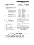
Figure 1.1: WCET Framework
Dealing with binary executables, the question arises whether an ICFG is really available
and whether this ICFG is really safe. Compilers often generate debug code containing
information about the ICFG of the program. Unfortunately, though, one usually cannot
always assume that this information is correct. Due to code optimisations the compiler
may have performed, the hints about the ICFG often only correspond vaguely with
reality.
It is even more unfortunate that executables for real-time systems most likely have no
debug information at all, at least not for all parts, since hand-written assembly code is
often included. E. g., hand-written assembly code can certainly be found in the realtime operating system, which is part of the statically linked executable.
In this work, an approach to a safe and precise ICFG reconstruction for real-time system
analysis will be presented. The reconstruction problem will be discussed in detail in
Chapter 4.
1.3 Path Analysis
Our analysis framework for predicting the worst-case execution time (WCET) of binary
executables for real-time systems is depicted in Figure 1.1. A WCET analysis can be split
into two basic steps.
The first step is the microarchitecture analysis. The result of the first step is a worst-case
execution time for each basic block of the program under examination.
The microarchitecture analysis consists of a chain of sub-analyses for different parts of
the hardware, like value analysis (to find values of registers, in particular addresses for
memory access), cache, pipeline and memory bus analyses. In our framework, all these
28
1.3. Path Analysis
analyses are implemented with the PAG tool (see [Martin, 1995b; Martin, 1999b]), that
uses Abstract Interpretation (AI) (see [Cousot and Cousot, 1977a; Nielson et al., 1999])
for analysis.
The second step of a WCET analysis is the worst-case path analysis. Based on the results
of the microarchitecture analysis, it computes an upper bound of the actual WCET. We
will call this the predicted WCET in the following.
Path analyses can be implemented in several ways. Because of good precision and
speed, we use Implicit Path Enumeration (IPE) (see [Li et al., 1995a; Li et al., 1996]),
which uses Integer Linear Programming (ILP) (see [Chvátal, 1983]) to find the WCET.
In this approach, the ICFG of the program is represented by a set of linear constraints.
Further, the objective function contains the execution time of each block of the program.
Then, finding the predicted WCET is the problem of maximising the objective function.
Chapter 7 will introduce this technique in detail.
Due to important deviation in whether routines are executed in isolation or in contexts,
routine invocations can be distinguished by their execution history, e. g., by their call
stacks as distinctive features. These distinctions are called execution contexts. The precise
methods of assigning contexts will be introduced in Chapter 3 and Chapter 8.
To make use of contexts, the original ICFG is transformed into one where nodes are
split according to their distinctive contexts. The resulting graph, the ICFG with contexts,
is then used for analysis instead of the original graph without contexts.
Our work group’s PAG tool for writing analyses using Abstract Interpretation comes
with interprocedural analysis methods, so ICFGs with contexts are can be used directly
by the microarchitecture analysis chain.
Up to now, ILP-based path analysis was not well adapted to interprocedural analysis
methods. It was shown in previous work (see [Theiling et al., 2000]) that it is possible in principle to combine microarchitecture analysis by Abstract Interpretation with
path analysis by IPE. However, ways of using arbitrary methods of context computation
were still unexamined. Chapter 8 proposes a general method of combining interprocedural analysis methods with ILP-based path analysis.
The task is non-trivial. ILP-based path analysis generates an objective function and some
sets of constraints of the following types:
Entry constraints. These state that the program entry is executed once.
Structural constraints. These describe incoming and outgoing control flow at each basic block.1
1A
basic block is a sequence of instructions in which control flow enters only at the beginning and
leaves at the end with no possibility of branching except at the end.
29
Chapter 1. Introduction
Loop bound constraints. Each loop needs a maximal iteration count to make the ILP
bounded. For good precision of analysis of loops, context distinction is desirable
for different iterations. This is made possible by transforming loops into tail recursive functions, so that interprocedural analysis methods become applicable.
User defined additional constraints. To improve precision by adding facts the user
knows to the set of constraints.
Most of these constraints can be generated in a straight-forward way even for graphs
with contexts. However, recursion poses a problem, since the presence of contexts restructures the analysis graphs w.r.t. the structure of cycles: entry and back edges of
cycles in the original graph are not necessarily entry and back edges of cycles in the
graph with context. Hence, a correspondence has to be found.
Chapter 8 will present how interprocedural analysis methods can be used for ILP-based
path analysis, dealing with the trade-off between analysis precision and speed. On the
one hand, high precision by using many contexts is desired, but one the other hand,
a distinction by the whole execution history is usually too expensive. For best results,
context computation should be as flexible as possible and should be limitable and adjustable for different programs under examination. Therefore, we will outline an algorithm for generating constraints, especially loop bound constraints, for ILP-based path
analyses with arbitrary static context computations.
1.4 Scope of this Thesis
We needed ICFGs in a framework for WCET analysis for real-time systems.2
In this thesis, I focus on the problem of constructing ICFGs for that WCET analysis
framework. I will identify the requirements for real-time systems and present safe, precise and also fast algorithms.
Further, I introduce a novel approach to interprocedural path analysis. Among other
things, this will show that the reconstructed ICFGs are perfectly suited for WCET analysis for real-time systems.
Consequently, this document is split into two major parts:
1. The design and implementation of novel algorithms for ICFG reconstruction will be
presented in the first part. The modular and versatile tool exec2crl is the result.
2 Our work group was partially supported by the research project Transferbereich 14, Runtime Guarantees
for Modern Architectures by Abstract Interpretation, 1999–2001, of Deutsche Forschungsgemeinschaft.
30
1.4. Scope of this Thesis
2. A new approach to interprocedural path analysis will be introduced in the second
part. The approach is much more generic than previous work.
The following list is a detailed overview of the structure of this work.
Part 1 contains chapters that introduce basic notations, terms and methods.
Chapter 2 introduces basic symbols and terms used in the following chapters.
Chapter 3 describes control flow graphs with their special properties and requirements for real-time system analysis. Also, methods of interprocedural analysis are introduced here.
Part 2 contains chapters that describe different stages of ICFG reconstruction implemented in our reconstruction tool exec2crl.
Chapter 4 describes the steps that are performed during a safe and precise extraction of control flow from binary executables.
Chapter 5 outlines the algorithms that are used to automatically transform a vendor’s machine description into a very efficient data structure that can be used
for classifying single machine instructions.
Chapter 6 presents the core of exec2crl, i. e., the algorithms it uses to safely reconstruct the whole ICFG of a program from instruction classifications.
Part 3 contains chapters that present the interprocedural path analysis developed for
our analysis framework.
Chapter 7 introduces the well-known technique of implicit path enumeration
(IPE) that is widely used today for implementing path analyses.
Chapter 8 presents our novel extension to IPE for interprocedural analysis.
Part 4 contains chapters that evaluate my work.
Chapter 9 presents the experimental results.
Chapter 10 concludes this work and discusses possible future work.
Chapter 11 relates this work to that of other researchers.
Appendix A depicts many control flow graphs to show how loop constraints are
generated in many different situations.
31
32
Chapter 2
Basics
This chapter will introduce basic symbols and notations that will be used in the following chapters.
2.1 Selected Mathematical Notations
This section clarifies in brief words the usage of some mathematical symbols in this
work. This section is not exhaustive, but only mentions some symbols that might be
unclear. Mathematical notation is assumed to be known to the reader.
Definition 2.1 (Tuples)
For an arbitrary domain D and for elements d1 d2 dn
written in two possible notations:
unrolled way: d1 d2 dn
indexed way: di
D, the according n-tuple is
i 1 n The domain of tuples of length n is written D1 n :
D1 n : di
i 1 n di
D
(2.1)
The empty tuple will be written ε.
33
Chapter 2. Basics
In contrast to this, the domain of vectors of length n is written Dn :
Dn : d1
.. .
dn
di
(2.2)
D
Definition 2.2 (Kleene Closure)
Given an arbitrary domain D, we define:
D
D1 n
(2.3)
ε
(2.4)
n D
D Definition 2.3 (Powerset)
For an arbitrary domain D, let D be its power set, i. e., the set of all subsets of D.
Definition 2.4 (Image)
Given a function f : M is defined as follows.
(2.5)
D : D D D N and a set M M, the image of M will be written f M and
f M :
f m
m
M
(2.6)
The image of f is the special case f M .
2.2 Program Structure
This section introduces notations that are used to analyse programs. The structure of
programs under examination will be clarified.
Let the program under examination be called P .
2.2.1 Programs and Instructions
Analyses work on programs, which are given as a sequence of instructions. Instructions
are either machine instructions, as is often the case for real-time system analysis, or more
generally minimal statements in the language the analysis works on.
Depending on control flow, the given sequence of instructions is split into basic blocks,
which are the basics of analysis.
34
2.2. Program Structure
2.2.2 Basic Blocks
The control flow of the program under examination is defined by jump instructions,
which are intraprocedural branches, and call instructions, which are interprocedural
branches. The branches divide the program into basic blocks, which control flow enters
at the beginning and leaves at the end, without the possibility of branching except for
the end of the basic block.
Let the set of basic blocks be V . This set must be finite: V ∞.
The reconstruction of control flow includes finding the division into basic blocks. For
raw machine code, this is not trivial. It is one topic of this work and will be described
in detail in Chapter 6.
In the scope of this work, we will use the following terms. The following terms will be
intuitively introduced now and clarified with
2.2.3 Routines
Structuring a program into smaller pieces of code is done in order to re-use parts of the
program (usually parameterised) and to get a nicer structure. These re-usable pieces of
code will be called routines. The words ‘function’ and ‘procedure’ occur in literature as
well, but this document keeps using ‘routine’ for the program substructures in order to
avoid confusion with mathematical functions.
Let R be the set of routines of P and let r0 be the routine to be invoked upon the start of
P , i. e., r0 is the main routine of P .
Every basic block belongs to exactly one routine. Let the function rout : V each basic block with its routine.
Let V f be the set of basic blocks of each routine: V f
v
V rout v
R associate
f .
Every routine has exactly one basic block that is the first to be executed upon invocation.
Let this basic block be called the routine’s start node. The set V contains all start
nodes of P , one for each routine.
Let there be a function
: R (2.7)
that associates the start node with its routine.
Another set of interesting basic blocks is constituted by those that contain routines invocations. These basic blocks are called call nodes. Let the set V contain all call
nodes of P .
The following function associates call nodes with their invoked start nodes. Call nodes
35
Chapter 2. Basics
may be associated with more than one start node, if there is more than one possible
routine to be invoked. This happens for computed calls.
The function will be defined for all nodes for convenience and returns
nodes.
: V v v
for non-call
(2.8)
V v invokes v
2.2.4 Control Flow Graph
Each routine has its own control flow graph, consisting of nodes that are basic blocks,
and edges representing the control flow between the blocks.
Let CFG f
Vf E f
f
R be the control flow graph of routine f .
As mentioned before, a control flow graph has exactly one start node f via which
all control flow enters routine f .
For a path in a graph G, e. g. in CFG f , from node v1 to v2 , we will write v1 v2 .
G
Definition 2.5 (Branch, Jump, Call)
If control flow has several alternative possibilities to continue at run-time after a given
basic block, i. e., if a node in a graph has several out-going edges, this situation will be
called a branch.
Branches in control flow graphs will be called jumps.
Branches in call graphs will be called calls or subroutine calls or subroutine invocations.
Call graphs will be defined now.
2.2.5 Call Graph
An important structure is a call graph. It is the graph that connects call nodes and start
nodes. It is defined by structures already defined: and constitute the nodes,
and restricted to defines the intraprocedural edges. The linkage between
start and call nodes is established by adding edges from start to call nodes for each
routine. Formally, we define the following.
36
2.2. Program Structure
c1
a()
main()
c2
b()
c3
Figure 2.1: CG (without context) of Example 2.2.6. Start nodes are labelled with the
name of the routine and a pair of parentheses, call nodes are labelled as shown in the
comment in the C source code. Note that our CGs contain no return edges, only call
edges.
Definition 2.6 (Call Graph)
Let CG V̂ Ê V̂ Ê V̂
as follows.
V̂ be the call graph of P , where Ê is defined
Ê
f F
:
s c
c s :c s c : s c :
s
CFG
f
c
It is required that call nodes have exactly one incoming edge in the CFG. This can be ensured by inserting additional empty nodes for the call nodes that contradict this requirement (the PAG framework does this). This way, together with the above definitions, each
call node c also has exactly one outgoing edge in the CFG. In the CG, c also has exactly
one incoming edge (from the start node) and possibly several outgoing edges (defined
by c ).
2.2.6 Example in C
void a() {
...
//
}
void b() {
a(); //
}
int main() {
a(); //
b(); //
}
basic block b1
invocation c3
invocation c1
invocation c2
Figure 2.1 shows the call graph of this short program.
Note 1: Definitions of call graphs in other literature often connect routines instead of
start and call nodes. However, the call graphs that we are going to use have to distin37
Chapter 2. Basics
a
a
b
c
b
c
loop
entry
node
local
d
d
back
node
exit
node
start nodes (CG & CFG)
call nodes (CG & CFG)
CFG only nodes
routines
CG edges
CFG edges
Figure 2.2: CFG modifications by loop transformation. The loop transformation introduces a new routine and new call nodes for each loop and transforms the loop into a
recursive routine. Dashed lines represent edges in the call graph, which are introduced
by this transformation.
guish call nodes, too. To get the call graphs used in other literature – those that connect
routines – simply form super nodes from start and call nodes of the same routine. This
way each node corresponds to a routine.
2.2.7 Loops
The term ‘loop’ will be used for a natural loop as defined in [Aho et al., 1986]. A natural
loops has two basic properties:
1. A natural loop has exactly one start node which is executed every time the loop iterates. This node is called header.
2. A natural loop is repeatable, i. e., there is a path back to the header.
We handle loops and recursion uniformly in our approach. This is done by transforming
all loops into recursive routines by making the loop body a routine on its own and
inserting interprocedural edges accordingly. The loop transformation that is used to
transform loops into routines uses an algorithm from [Lengauer and Tarjan, 1979] to
find and extract loops.
Figure 2.2 depicts a loop transformation.
Apart from loops, there must be no other cycles in the control flow graphs. Although
this is a restriction, compiled code and well-done hand written assembly code will not
use other types of cyclic control flow. The reason for this restriction is the unbounded
run-time of control flow cycles. When the path analysis searches the maximal run-time,
loops must be bounded with maximal iteration counts in order to make the problem
38
2.2. Program Structure
loop entry node
entry edge
loop header
exit edge
back edge
back node
exit node
Figure 2.3: A simple loop with all the important edges. Dotted lines and white nodes
are in the call graph, the other items are part of the control flow graph
solvable. Because only loop iteration counts are specifiable, only these types of cycles
are currently allowed.
After loop transformation, there must be no cycles in the control flow graphs at all. All
cycles must have been moved to the call graph and marked as loops.
Let L be the set of loops of program P . Because loops are converted into recursive
routines in our framework, it holds that L R. Therefore, the header of a loop is simply
the start node of the loop. Still, we define a function that assigns the header to a loop
for clarity.
Definition 2.7 (Loop Header)
The header of a loop l L is defined as follows.
header : L l l
(2.9)
Figure 2.3 shows a simple loop.
Because loops and recursion are the same in our framework, there may be more than
one entry for a loop. This case occurs when a recursive routine is invoked from several
different call sites. A more complex example of a loop is shown in Figure 2.4 on the next
page.
39
Chapter 2. Basics
loop entry node
back edge
back edge
loop entry node
entry edge
entry edge
loop header
back node
back node
Figure 2.4: Complex recursion, CG only. The loop is entered from two call sites. One of
the entry nodes also has an outgoing edge that calls a non-involved routine. There are
two back edges, one of which recurses via another function call. Further, one of the back
nodes has two outgoing edges, but only one is a back edge. To handle all this, much
care has to be taken.
40
2.3. Integer Linear Programming
Definition 2.8 (Entry Edges)
Let there be a function
entries : L Ê
(2.10)
that assigns to a loop its entry edges.
Let there also be a function that returns the set of back edges of the loop, i. e. those edges
that enter the loop from inside the loop. Note that usage of ‘inside’ here refers to nested
re-invocations of the loop as well.
Definition 2.9 (Back Edges)
back : L Ê
(2.11)
The number of iterations of loops will be specified using two functions. One for the
minimum iteration count and one for the maximum. The iteration bounds will be defined for each entry of the loop and, therefore, the two functions take and loop entry node
as their argument.
Definition 2.10 (Minimum and Maximum Loop Iteration Count)
Let l be a loop and e entries l one of its entry edges.
The minimum loop execution count per entrance of l via e will be written nmin e .
The maximum loop execution count per entrance of l via e will be written nmax e .
2.3 Integer Linear Programming
This section introduces the basics of Integer Linear Programming (ILP) briefly. A precise
description of the underlying theory can be found in many books (see [Chvátal, 1983;
Schrijver, 1996; Nemhauser and Wolsey, 1988]).
2.3.1 Linear Programs
This section introduces the structure of Linear Programs. How they can be solved will
be shown in the next section.
Definition 2.11 (Comparison of Vectors)
Let ∆ be a comparison operator and let a b
a ∆ b :
n.
Then we define
ai ∆ bi i 1 n
41
Chapter 2. Basics
Definition 2.12 (Linear Combination)
n
n
Let x
be variable and let a
be constant. Then aT x is called the linear combination
of x.
Definition 2.13 (Linear Program)
d
m
m d
be known and constant. A Linear Program (LP) is the task
b
A
Let t
d
T
to maximise t x in such a way that x
A x b. In short, this is written:
0
max : t T x A x
Definition 2.14
In Definition 2.13 the function C :
d b x
d
where C x
0
t T x is called objective function.
The inequalities given by A x b are called constraints. x is said to be a feasible solution,
d
if it satisfies A x b. Let P x
b be the set of feasible solutions of x. x is
0 Ax
T
said to be an optimal solution, if t x max t T x x P .
To reduce a problem of minimising to one of maximising, the objective function can be
multiplied by 1.
Further, the constraints that are used in the definition of a Linear Program are of the
form ak 1 x1 ak 2 x2
ak d xd bk . Other types of constraints like
a k 1 x1
where ∆
mations:
ak d xd ∆ ak 1 x1
ak e xd
(2.12)
can be reduced to the basic form by using the following transfor-
1. Instead of ∑1 ∆ ∑2 write ∑1 ∑2 ∆ 0.
2. Instead of ∑ 0 write ∑ 0.
3. Instead of ∑ 0 write ∑ 0 and add the constraint
∑
0.
There are three cases that can occur when an LP is tried to be solved:
1. P : The LP is infeasible.
2. P , but sup t T x x P . The LP is unbounded.
3. P , and max t T x x P . The LP is feasible and has a finite solution.
To find the solution of a linear program, upper bounds of the objective function must be
computed. The problem of finding the least upper bound is also an LP that is defined
as follows.
42
2.3. Integer Linear Programming
Definition 2.15 (Primal and Dual Problem)
d
Let max : t T x A x b x
0 be a Linear Program. Let this program be called primal
problem. The dual problem is the problem of finding the least upper bound of t T x, which
d
is defined as follows: min : yT b yT A t T y
0.
The two following theorems hold (Duality Theorems of Linear Programming):
Theorem 2.16 (Weak Duality)
Let x̄ be a feasible solution of the primal problem max : t T x A x
a feasible solution of its dual problem min : yT b yT A t T y
d and let ȳ be
b x
0
d . Then it holds that:
0
ȳT b t T x̄
Theorem 2.17 (Strong Duality)
d
Let x be a feasible solution of the primal problem max : t T x A x b x
0 and be y d
T
T
T
be a feasible solution of its dual problem min : y b y A t y
0 . Then it holds
that:
y T b t T x
x and y are optimal
Corollaries
If the primal problem is unbounded, the dual problem is infeasible.
If there are feasible solutions of the primal and the dual problems, then there is
an optimal solution. The values of the objective function of the two problems are
equal for the optimal solution.
The following Simplex algorithm exploits that for a feasible preliminary solution x of the
primal problem, there is a solution y of the dual problem. If that solution is feasible
in the dual problem, it is optimal (due to the second corollary). If it is not, the basic
solution can be improved.
2.3.2 Simplex Algorithm
This section introduces a non-formal description of the Simplex algorithm. There is a
vast amount of literature about LP solving and the Simplex algorithm available for the
interested reader, e. g. [Chvátal, 1983; Schrijver, 1996; Nemhauser and Wolsey, 1988].
The constraints of a linear program isolate a convex area in n 0 . An optimal solution
is found in one of the corners of this area. Starting with an arbitrary corner, a better
43
Chapter 2. Basics
Optimum
x2
Steps of the Simplex algorithm
Direction of optimisation
Basic solution
x1
Figure 2.5: The Simplex algorithm in 2 0 .
solution of the objective function is searched by following one of the outgoing edges of
that corner. This is repeated until no adjacent corner has a better value, which means
that the optimal solution has been found. Figure 2.5 on the next page illustrates this
algorithm.
The simplex algorithm can be used to solve large problems, since for most applications,
its runtime is O m for m constraints. However, constraints can be constructed so that the
algorithm performs in only O 2m time (e. g. the Klee Minty cube (see [Chvátal, 1983])).
There are better algorithms from the complexity point of view, e. g. the Ellipsoid method
or the Projective Scaling Algorithm by Karmarker, which have polynomial run-time.
2.3.3 Integer Linear Programs
Many problems only allow integer solutions for the solutions of an LP, i. e., in Defini
d . And because we already made
tion 2.13 on page 42 it must additionally hold that x
d.
the restriction that x 0, it must even hold that x
0
This type of constraint will be needed for the algorithms in Chapter 7, where the variables of the LP are execution counts of basic block, which are naturally integers.
Definition 2.18 (Integer Linear Program)
d
m
m d
Let t
b
A
be constant and known. An integer linear program (ILP) is
d Ax
b.
the task to maximise t T x in such a way that x
0
max : t T x A x
b x
d
0
To find a solution of an ILP, additional steps have to be taken, because the Simplex algorithm (and others for LP solving) cannot be used directly, since the additional restriction
44
2.3. Integer Linear Programming
Feasible solutions of the ILP
x2
Feasible solutions of the LP
x1
Figure 2.6: Domain of feasibility of an ILPs (grid points) and corresponding domain of
feasibility of the LP-relaxed problem (shaded area).
to integer variable cannot be handled by them. Actually, it is N P -complete to solve ILPs.
However, in practice, many large ILPs problems are solvable with a moderate amount
of effort.
Definition 2.19 (LP-Relaxed Problem)
d be an Integer Linear Program. Then max : t T x A x
Let max : t T x A x b x
b x
0
d
0 is said to be the corresponding LP-relaxed problem. In the following, it will also be
called relaxed problem.
The relaxed problem is used to solve ILPs. It does not contain demands for integer
variables and all feasible solutions of the ILP are also feasible for the LP. I. e., starting
from the LP the integer property of all variables is tried to be achieved. The following
algorithm works like that.
2.3.4 Branch and Bound Algorithm
The basic idea of the Branch and Bound Algorithm is to solve the relaxed LP and then
split the domain of feasibility into two sub-problems in order to satisfy the demand for
integer variables. Each sub-problem is then solved until all variables are integers.
Let Ψ be an ILP and let Ψ be the relaxed problem. If it is feasible, solving Ψ yields a
d
solution x̂
0.
d , so a solution is found for Ψ, too. If not a coordinate i
1 n is chosen such
If x̂
that x̂i
. The two sub-problems Ψ̃1 and Ψ̃2 are created from Ψ by adding one of the
following inequalities:
xi
xi x̂i
x̂i
(2.13)
(2.14)
45
Chapter 2. Basics
These constraints exclude x̂ as a solution for Ψ̃1 and Ψ̃2 . This method is repeated until
all variables are integers.
No word was said about major problems and methods used in this algorithm, such
as how to choose a coordinate, or which order the sub-problems should be solved in.
Again, interested readers should refer to standard literature like [Chvátal, 1983; Schrijver, 1996; Nemhauser and Wolsey, 1988].
There are freely available tools like lp solve1 that implement very good algorithms
for solving ILPs. lp solve was used for this thesis.
1 lp
solve
was
written
by
Michel
ftp://ftp.es.ele.tue.nl/pub/lp solve.
46
Berkelaar
and
is
freely
available
at
Chapter 3
Control Flow Graphs
While the previous chapter has already introduced basics about programs, their control
flow graphs and call graphs, this chapter will describe in detail the precise structure
of the control flow graphs our framework uses. Requirements of CFGs and CGs for
real-time system analysis will be discussed.
3.1 Control Flow Graphs for Real-Time System Analysis
To talk about control flow graphs and call graphs simultaneously, the term interprocedural control flow graph (ICFG) will be used to refer to all control flow graphs and to the call
graph of a program.
Real-time system analysis requires safe and precise analysis methods. Safety has the
highest priority since real-time systems are usually part of a large, safety-critical environment where errors can lead to fatal damage, as mentioned already in the introductory chapter.
3.1.1 Safety
For our WCET analysis framework, this means that all analyses must be based on a safe
ICFG in the first place. If the ICFG is unsafe, the whole analysis chain will be unsafe.
47
Chapter 3. Control Flow Graphs
To define safety for ICFGs, it must be thought about what unsafety means, since ICFGs
seem to be something that either represents a program, or which does not, in which
case it must be said to be incorrect. It is not that simple, however, since control flow
is sometimes unclear or unpredictable for analyses. Of course, our first requirement is
correctness. This is more than obvious:
A safe interprocedural control flow graph must be correct.
Secondly, if any uncertain control flow is encountered, it must be clearly marked for
analyses to be able to react to uncertain control flow.
A safe interprocedural control flow graph must mark uncertainties clearly.
Subsequent chapters will reason about how to achieve these goals when reconstructing
control flow. This chapter will focus on the precise structure of ICFGs and on how the
required information can be made available to analyses.
3.1.2 Precision
For analyses to be precise, the underlying ICFGs must be precise, too. Whenever control
flow can be represented precisely or imprecisely, this chapter will discuss that topic.
Precision in control flow is usually an issue for alternative flow, i. e., where the final
taken alternative is decided at run-time. Examples are computed jumps (e. g. switch tables) or computed calls (e. g. function pointers or virtual function calls in object-oriented
languages). The issue is usually a question of infeasibility: more precision means to be
able to predict statically which alternative paths are really infeasible. The more this can
be predicted, the more precise the ICFG will be.
3.2 Detailed Structure of CFG and CG
This section describes the precise structure of the ICFGs that are used in this thesis. It is
a clarification of the data structures presented in Chapter 2.
The graphs that are used are based on those provided by the PAG framework. However, the graphs used here are computed from the PAG graphs to suite the needs of the
presented algorithms best. This section will clarify how these graphs look like.
In order to prevent special cases, like conditional calls, etc., our CFGs and CGs contain
additional empty basic blocks at specific locations, i. e., when routines are invoked and
left. Because of loops being transformed to recursion, these empty blocks also help to
avoid special cases here, e. g., there cannot be two loops starting before the same basic
block. This can be programmed in Pascal with two nested repeat loops.
48
3.2. Detailed Structure of CFG and CG
f1()
f2()
start
start
CG edges
CFG edges
...
call
instr.
CG, CFG nodes
call
CFG only nodes
call
local
...
return
...
exit
exit
Figure 3.1: CFG and CG of a call of a recursive routine. The two graphs are shown in
one figure. This figure clarifies the use of local edges and shows that there are no return
edges (e. g. from a node in routine f2 back to the call node in f1).
Four types of empty nodes exist: at each routine invocation, two additional empty
nodes are inserted: a call node and a return node. The actual call instruction is located in
the block before the call node. Routines begin with an empty start node and returning
control flow is gathered in a unique exit node.
Our CFGs contain a local edge after each call node, because the call graphs will not
contain flow information about routine returns. This is the most convenient way of
representation for the analyses that will be described later (see Section 7.3.3 on page 113).
A routine call with all important nodes is depicted in Figure 3.1.
3.2.1 Alternative Control Flow and Edge Types
Alternative control flow occurs at two levels: in the control flow graph, where if-thenelse statements are the most common example, followed by switch-statements, and in
the call graph, where function pointers are the most common example. Virtual function
calls are usually a special case of function pointers.
To handle alternative control flow in control flow graphs, there are different types of
edges. Some analyses need this edge type in order to compute the correct behaviour.
E. g. jumps often have different execution times for different types of edges.
We formally define the edge type as a function that assigns a type to each edge.
49
Chapter 3. Control Flow Graphs
Definition 3.1 (Edge type)
Let type : E normal false true local normal edge: outgoing edge of basic blocks whose control flow exits without alternatives (i. e., without a branch)
false edge: for a conditional jump, this marks the edge that is taken if the branch is not
taken. This type of edge is also known as a fall-through edge. At each block, there
is maximally one of these edges.
true edge: for a jump, this marks possible branch targets of the jump.
local edge: this edge was introduced in the previous section: it is the representation of
control flow after a call.
For switch tables, there may be a number of true edges, one for each possible branch
target.
Alternative control flow in the call graph is marked in the same way by using multiple
outgoing edges from a call node to several start nodes.
3.2.2 Unrevealed Control Flow
If any control flow is unknown, it is required that the control flow graph contains information about this. This is vital for analyses, since they might analyse to the wrong
thing.
Unrevealed control flow, i. e., edges that are known to exist but with an unknown target,
can be marked at the basic block to have additional successors in the control flow graph
or the call graph. We introduce two sets to account for this.
Definition 3.2 (Unrevealed edges)
Let be the set of call nodes that contain instruction with unknown call targets. Because we cannot have edges with an unknown target, we use this set instead.
For a given routine f , let Ṽ f V f be the set of basic block that contain instructions with
unknown jump targets.
3.2.3 Calls
Modern architectures and run-time libraries have several interesting peculiarities that
have to be thought about. Many of these peculiarities showed up when the control flow
50
3.2. Detailed Structure of CFG and CG
a)
b1
normal
true
start 1
call
false
...
return
...
start n
normal
b2
b2
b1
true
call
false
start 2
local
return
start n
normal
start 1
call
start 2
local
b)
b1
local
return
b2
c)
d)
b1
true
start 1
start 2
...
call
false
local
return
start n
normal
b2
start 1
start 2
...
start n
exit
Figure 3.2: Different types of calls and their representation in the ICFG. a) normal call
(with several alternative targets), b) conditional call, c) conditional no-return call, e)
conditional immediate-return call
51
Chapter 3. Control Flow Graphs
reconstruction algorithms (see Chapter 6) were implemented for different targets. Calls
are more complex than normal jumps, since they involve the mechanism of returning
to the caller, so the fall-through edge has a totally different meaning for calls than for
jumps. Therefore, the generation of edges needs to be clarified for the interprocedural
case as well as for the intraprocedural case.
In the course of the examination of different programs, libraries and architectures, we
found the need to distinguish the following types of calls. The categories listed below
are not mutually exclusive.
computed calls: calls that use the value of a register as a branch target. These usually
result in alternative control flow.
unpredictable calls: calls that have unrevealed call targets.
conditional calls: calls that may possibly not be taken.
not-taken calls: calls that are never taken
no-return calls: calls that never return, e. g., because they invoke a routine that implements an infinite loop, or calls to a system function that exits the program.
immediate-return calls: calls that end the current function immediately when they return.
Handling of computed calls and unpredictable calls has been described already above.
Calls that are not taken are represented by having no call nodes at all.
Whether a call is conditional, not-taken, no-return or immediate-return is represented
by edges in the control flow graph. One interesting fact is that calls might not return to
the caller, but branch to somewhere else when they return. This is the case for no-return
and immediate-return calls.
Figure 3.2 on the previous page shows the ICFGs associated with different types of calls.
3.2.4 External Routines
External routine calls are frequent and should be handled by any WCET analysis framework. Our approach is to introduce a basic block of the type external, which represents
the execution of the external routine. It is like a black box.
Analyses can decide how to handle these external basic block nodes. The WCET analysis will have to assume that the run-time of such blocks is known, so either a library of
pre-analysed run-times is needed, or the user has to be queried.
52
3.2. Detailed Structure of CFG and CG
external routine
call
start
external
exit
Figure 3.3: External routine call: an external node is introduced that represents the external routine as a black box.
3.2.5 Difficult Control Flow
Programmers may use strange concepts of structure and produce something that is executable, but with weird control flow. This chapter deals with these cases.
Examples of weird, or better difficult control flow are the following.
Jumps into loops past the loop header.
Entering routines at different basic blocks.
Unfortunately, even so-called high-level programming languages sometimes support
the generation of structures that are difficult. E. g. most imperative programming languages support a goto command that allows for jumping to any point in the current
procedure. This way entering loops past the header is possible.
Some old imperative languages that are still in wide use, like C, even do not enforce a
clear block-structure for their own structuring mechanisms. E. g., while and case statements need not be nested correctly, triggering the same problem of entering loops past
the header. An infamous example is Duff’s device, used to unroll a typical memory
copy loop and interlace it with the initial aligning case. This is shown in Figure 3.4 on
the next page.
Many cycles that are not natural loops could be transformed into a natural loop by
unrolling them once. Duff’s device is one example for this. Usually, it is not clear which
block should be the loop header then, because with different entries it is unclear which
block inside the loop is executed as many times as the loop is executed.
The second example, entering routines at several basic blocks can usually only be programmed when using the assembly or machine language directly. Although this is assumed to be very bad coding style, it can often be reconstructed to nice control flow by
53
Chapter 3. Control Flow Graphs
unsigned int n = (count + 7) / 8;
switch (count % 8)
do
case 0: *to++ = *from++;
case 7: *to++ = *from++;
case 6: *to++ = *from++;
case 5: *to++ = *from++;
case 4: *to++ = *from++;
case 3: *to++ = *from++;
case 2: *to++ = *from++;
case 1: *to++ = *from++;
while (--n > 0);
Figure 3.4: Duff’s device. The loop is entered at several points by interlacing switch
statement and while loop in C.
introducing additional routines (e. g., when the same routine tail is used by two routines, this tail can be made a routine on its own if no jumps leave that new routine).
However, such a structure cannot always be reduced to nice control flow, so a full automation cannot be expected. Therefore, it seems unwise to start implementing without
observing the important special cases that should be handled automatically. Our framework is very flexible to easily allow such extensions as soon as they are encountered.
3.3 Contexts
Contexts were introduced in previous work already. They were used for analysis with
the PAG framework and described in most detail in [Martin et al., 1998] and [Martin,
1999b]. This section gives a brief introduction needed to understand the subsequent
chapters. Further, the newest development of our analysis framework is outlined by
presenting the VIVU n k context mapping with customised unrolling.
Our analysis framework provides the possibility of categorising different executions
of basic blocks by the control flow that led to its execution. These classes are called
contexts. Each basic block must only be assigned a finite number of contexts to ensure
the termination of the analysis.
There are different approaches for assigning contexts.
By the value of parameters. The idea is that routine invocations that use the same pa54
3.3. Contexts
rameters are identical for the analysis. This approach is called functional approach.
This technique may be used for analyses using Abstract Interpretation. The distinction criterion of routines is rather the abstract value of the analysis than the
parameters of the routine. For this analysis method to yield only a finite number
of contexts, the abstract domain must be finite, which is a limitation.
However, one problem with the functional approach is the potentially large number of contexts that is unknown before the analysis. Further, the contexts are computed dynamically during the course of the analysis and cannot be re-used in subsequent analyses since different abstract domains are usually used.
By the routine invocation history. These routine invocations used for context computation are specified in the call graph. Therefore, this approach is called call graph
approach.
Since the routine invocations are known before the analysis starts, the contexts can
be computed statically with this approach. So this approach is easily applicable to
multi-stage analyses where several sub-analyses can use the same set of contexts.
Throughout our framework for WCET analysis, the call graph approach is used for analyses. Any other static approaches of context computation could be used as well.
Contexts are computed in different ways, depending on the desired level of precision
and the acceptable computation effort for the specific analysis problem. The computation depends on the execution history by which the basic block is reached. The computation of contexts will be called a mapping and will be defined formally below.
Mappings that follow the call graph approach are finite abstractions of all possible call
histories of a routine. The call history of a routine can be represented by a string of call
edges that represent the path of the invocation of that routine. This string is called call
string.
Definition 3.3
Let S Ê be the set of call strings.
Of course, with the presence of recursion, S may be infinite. An operator is used to
compute a finite set of contexts for a set of call strings. Like call strings, contexts are
also represented by strings, where the links of the strings are from a domain Θ̂, which
depends on the mapping. Elements from Θ̂ are called context links, in analogy with
chain links.
55
Chapter 3. Control Flow Graphs
Definition 3.4 (Mapping, Connector)
A mapping is a pair Θ̂
, where the context connector is a function
: Θ̂ Θ̂ Ê To compute a context from a call string, let be applied recursively to each call string
link.
f : S
Θ̂ (3.1)
s1 s2 sn ε s 1 s2
sn
Let the set of contexts Θ Θ̂ be the image of f .
Θ
f s s
S
is called a finite context connector, if Θ ∞.
All connectors will be demanded to be finite in the following. Therefore, the term connector will be used for a finite context connector as an abbreviation.
If it is clear from context, Θ will be written instead of Θ .
3.3.1 CallString k A very simple mapping is the CallString k mapping, which simply limits the length of
the call strings to k elements. Only the most recent call edges are considered for context
distinction.
First, we need the operation that limits strings to length k.
Definition 3.5 (Strings of limited length)
For an arbitrary domain D, let d k d D be defined as follows.
1 dn dn d1
dn dn dk dk k Definition 3.6 (CallString k )
Let CallString k Ê k , where k
e1 e2 en
0,
1 1 d1
d1
if n k
otherwise.
and
k en 1 e1 e2 en en
1 k
Since most calls only have a single target, instead of writing the edges in the call string,
it is common to only write the call nodes for simplicity.
56
3.3. Contexts
CallString 0 corresponds to non-interprocedural analysis, since all contexts have length
0 and, therefore, yield no context distinction at all.
Of course, k is a tuning factor to limit the complexity of the mapping to make the analyses perform well.
In Example 2.2.6, basic block b1 in routine a() is executed with two different call stacks:
c1 and c2 c3 depending on the control flow that led to the invocation of routine a.
Starting from CallString 2 , we thus get two contexts for basic block b1.
3.3.2 Graphs with Context
Connectors can be used to define new graphs, namely, control flow graphs and call
graphs with context. These graphs are the basis of all of our interprocedural analyses.
The call graph with context, CG , is defined as follows:
Definition 3.7 (Call graph with context)
Let Θ be the set of contexts and a finite context connector and let CG V̂ Ê be a
call graph and let f0 be its main routine. Recall from Definition 2.6 on page 37 that
V̂ .
Then a call graph with context is a graph CG : V̂ Ê , where V̂ V̂ Θ and Ê V̂
V̂ are defined recursively from V̂ and Ê, respectively, using the connector .
The main routine with the empty context is part of V̂ :
f0 ε
V̂ .
Edges from start nodes to call nodes do not change context:
vϑ
Ê
v ϑ
V̂ and
vϑ
v v
v ϑ
V̂ v
Ê .
Edges from call nodes to start nodes change context according to
vϑ
V̂ v
v ϑ
vϑ
v v
v v
v ϑ
Ê
:
V̂ and
v v
Ê .
The set of routines with context is a set of pairs of routines and all their corresponding
contexts.
57
Chapter 3. Control Flow Graphs
Definition 3.8 (Routine with context)
The set of contexts of a routine r is written Θ r . It is defined as follows:
Θ r :
ϑϑ
Θ r ϑ
V̂
The set R of routines with context r ϑ is defined as follows.
R : r ϑ
r
Rϑ
Θr
A control flow graph with context, CFG , is defined as follows:
Definition 3.9 (Control flow graph with context)
Let r ϑ R be a routine with context and let CFG f
of routine r.
A control flow graph with context is the graph CFG
Vr ϑ : v ϑ
r ϑ v
V f E f be the control flow graph
Vr ϑ Er ϑ , where
Vf and
Er ϑ : e ϑ
e
Ef Thus, control flow graphs with context are isomorphic to their corresponding, original
control flow graph without context. Their nodes are simply extended by a context.
For convenience, we combine all nodes of all graphs with context in one set.
Definition 3.10 (Set of all nodes)
Let V : Vr
r R
Accordingly, the set of all edges is defined as follows.
Definition 3.11 (Set of all edges)
Let E : Er
r R
58
3.3. Contexts
Definition 3.12 (Other structures with contexts)
The sets and are defined by distinguishing nodes from CG by a context:
Θ
Θ
:
:
V̂
V̂
Similar definitions apply to sets of unrevealed control flow.
:
:
Ṽr ϑ
V̂
Vr ϑ
Ṽr
Θ
Θ rϑ
R
Further, edge types do not change with the presence of contexts.
type e ϑ
:
type e
eϑ
E
Finally, in order to talk about the possible contexts of a node, we define the following.
Definition 3.13 (Set of Contexts of a Node)
The set of contexts that are distinguished for a given node v in a control flow graph with
context CFG will be written Θ v . It is defined as follows.
Θv
Θ rout v
3.3.3 Iteration Counts for Contexts
With the introduction of contexts, we allow the minimum and maximum iteration count
(see Definition 2.10 on page 41) to be defined per entry edge and per context. So we
extend nmin and nmax as follows.
The minimum loop execution count per entrance of that loop via an entry edge e Ê
will be written nmin e . The maximum loop execution count per entrance will be written
nmax e .
Figure 3.5 on the next page depicts the CG of Example 2.2.6. It can be seen from the figure that the CallString 2 CG is maximally precise w.r.t. control flow, i. e., no control flow
from two different calls ever joins in deeper calls. In contrast to this, in the CallString 0
CG on the right, control flow from the calls c1 and c2 joins when a() is invoked from
c3.
3.3.4 Recursive Example
This section will clarify how different mappings make different CGs . Consider the
following program:
59
Chapter 3. Control Flow Graphs
a(),
c1
a(),
c2
a(), ε
c3
main(), ε
main(), ε
c1,
ε
b(),
c2
c1,
ε
b(), ε
c2,
ε
c3,
c2
c2,
ε
c3, ε
Figure 3.5: CG : each node is a pair of basic block and context. a) on the left: CallString 2 ,
b) on the right: CallString 0 . b) is isomorphic to the CG of this program.
Example
void a (int x)
{ ...
a(x-1);
// c2
...
}
int main (int, char**)
{
...
a(5);
// c1
...
}
The contexts for CallString 2 and CallString 1 are as follows:
CallString 2
for main() ε
for a()
c1
c1 c2
c2 c2
CallString 1
ε
c1
c2
As can be seen, the ‘older’ parts of the execution history are chopped off.
3.3.5 VIVU n k For better precision of loop analysis, we have developed a mapping technique that distinguishes the first few iterations from all other iterations, which are joined in one context. By this, loops are virtually unrolled.
60
3.3. Contexts
To do this, the CallString k approach is modified to add a saturated counter to each context link in order to count how often a routine is recursively invoked.
Saturation of the counter is indicated by the symbol . Loop back nodes do not occur
in contexts anymore, but instead, the corresponding counter is incremented. VIVU n k
is the mapping where n distinctions are the maximum, i. e., the counter may have the
values 1 n 1 , and where the contexts may not be longer than k elements.
Several VIVU mappings have been introduced before (see [Martin, 1999b]). The VIVU
mapping that will be introduced here is the most recent development involving different loop unroll counts per loop.
The idea is that in the best case, a loop should be unrolled as often as it is maximally
iterated for maximal precision. Because there might be problems with complexity, an
unroll limit n is added to the mapping. 1
Definition 3.14 (Saturated Set of Positive Integers)
∞ , let
For n
n :
1 n
1
if n
,
otherwise.
Definition 3.15 (Saturated sum)
For n
, let i n j i
n j
0 be defined as follows.
i
n
j
i
j
if i i j n
otherwise.
With this definition, we can now define VIVU n k . Also recall that nmax e is the maximum loop iteration count.
Definition 3.16 (VIVU n k –“VIVU-4”)
Let Ê call : Ê , i. e., those CG edges that enter a routine.
1 In
the PAG framework, the style of mapping introduced here is known as VIVU-4. (And the version
where k is the constant unroll count for all loops is known as VIVU-ht).
61
Chapter 3. Control Flow Graphs
Let VIVU n k
c ν s ν iν
Ê call
k
n
ν 1 l c ν s ν iν
n
cl
k
n
, where k
s
1 l 1
ν 1 λ 1 c ν s ν iν
ν 1 l 1 k
0
∞ n
∞ , and
c λ s λ iλ
where il
if λ such that sλ sl 1
(use the minimal λ here)
otherwise.
min n nmax cλ sλ 1
:
1
1
n0
Note: the minimal λ in the first clause of the definition is used for formally getting a
complete definition: when successively generating contexts from ε, there is maximally
one such λ.
Claim 3.17
k is well-defined.
n
Proof
The only thing that might be unclear is why the saturated addition may be used without
problems, since n is allowed to be ∞.
To see this, see that min n nmax cλ sλ ∞ for any n, even if n ∞, since it is required
that a maximal loop bound is given for each loop. So nmax cλ sλ
∞ for every cλ .
Since most calls only have a single possible target, it is common to only write the call
nodes for simplicity instead of the complete call edge in the VIVU context links.
Because recursion is folded in the VIVU-approach by the introduction of a saturated
counter, VIVU generates finite context sets even if k ∞, since nothing but call graph
cycles, i. e. recursion, leads to infinite call strings. However, this has to be proven.
Claim 3.18
k is a finite context connector.
n
Proof
It must be shown that
k
n
produces finitely many contexts only.
Unfortunately, the underlying domain of context links Ê call
n is infinite for n ∞.
However, for any given loop entry edge e entries l l L, it holds that min n nmax e ∞.
So there is a maximum saturated index for each program, namely n0 : max min n nmax e e entries l l L ∞, since ∞. Therefore, for a given
call
call
program, context links are rather in Ê call
∞ and
n0 Ê
n . Because Ê
call
call
n0 ∞, it follows that Ê
Ê
n0 ∞.
n0 62
3.3. Contexts
What is left to be shown is that each context that can be produced has finite length. For
k ∞, this is clear. The maximum length is k in that case.
If k ∞, there are still only finitely many contexts, since by Definition 3.16 on the previous page, no edge with the same start node can occur twice in one context (because
these edges are collapsed by the use of a counter). So the maximal length of a context is
∞.
Figure 3.6 on the next page also shows a VIVU n k mapping for the example recursion
to show how the mapping works.
Most significantly, the counter element of VIVU n k prevents that the CG contains joins
for every recursion, because the contexts are not shifted, but simply a counter is incremented. This yields better precision w.r.t. execution history.
3.3.6 Example
void a(int i) {
...
a(...); // c3
...
}
int main() {
a (10);
// c1
a (20);
// c2
}
Figure 3.6 on the next page shows the CG and some CGs for different context mappings.
63
Chapter 3. Control Flow Graphs
a)
c1
a()
c2
c3
c1, ε
a(), c1
c3, c1
c2, ε
a(), c2
c3, c2
main(), ε
main()
c)
b)
c1, ε
a(), c1
a(), c3
c3, c1
a(), c1 c3
c3, c1 c3
a(), c3 c3
main(), ε
d)
c2, ε
a(), c2
c1, ε
a(), (c1, 1)
c3, (c1, 1)
a(), (c1, )
c3, (c1, )
c2, ε
a(), (c2, 1)
c3, (c2, 1)
a(), (c2, )
c3, (c2, )
c3, c2
a(), c2 c3
c3, c3
c3, c3 c3
c3, c2 c3
main(), ε
Figure 3.6: a) CG of Example 3.3.4. b) CG with CallString 1 mapping: the distinction
by the two calls from main() is always lost in a(), because of the recursion. c) CG
with CallString 2 : regardless of the maximum length, a() is never distinguished by
the call from main(). d) CG with VIVU 2 1 mapping: the two calls in main remain
distinguished in spite of the recursion.
64
Part II
Control Flow Graphs and Binary
Executables
Chapter 4
Introduction
Analyses for WCET prediction for real-time systems usually work on executable programs. The reason is that modern hardware involves techniques that are only predictable at a level close to hardware. Examples for these techniques are caches and
pipelines.
Caches improve execution time by storing recently used data. Reading and writing
to a cache is much faster than writing to main memory, therefore, assuming that
recently used data is likely to be used again, accesses can be sped up.
This additional store between the main memory and the processor (sometimes
organised in several layers with different sizes and access times) makes program
execution time depend on the execution history. For an analysis to be able to take
cache behaviour into account, it must know about accessed memory addresses.
Pipelines improve execution speed by overlapping the processing of subsequently executed instructions. Due to dependencies between instructions, this overlap is
usually not perfect, but instead, instructions sometimes stall until dependencies
are resolved. An example is an instruction that has to wait for a result of a previously executed instruction before it can use that result for its own computations.
Due to this, instructions’ execution times depend on the instructions that have
been executed before. Also, pipeline behaviour usually depends on cache behaviour, since if an instruction waits for data from main memory, dependencies
in the pipelines may be resolved in parallel.
67
Chapter 4. Introduction
To summarise, for modern architectures it is usually necessary for a precise analysis to
know memory access addresses. I. e., it is not sufficient to know the names of data and
code labels, but the precise addresses on the hardware should be known for making
precise predictions.
Therefore, statically linked executables where all the low-level information are typically
needed for a precise WCET analysis. The contrast to assembly or source code is as
follows:
Machine instructions. In assembly programs, one assembly instruction might correspond to several machine instructions, e. g., some processors contain specialised
versions of instructions where a register operand is fixed, which can be stored in
less space.
On source code level, there is no information at all about what instructions are
executed on the processor, since code generation is the task of the compiler. Particularly in the presence of sophisticated code optimisations, predictions about
generated machine instructions are usually not possible.
For WCET analysis, it is important to precisely know which machine instruction
is used, because the execution behaviour is different.
Addresses. On assembly level (also on higher levels), branches are specified by names,
i. e., labels. For most modern processors, WCET analysis needs the addresses that
the processor uses to predict its behaviour, since accesses to different addresses
may result in different execution times.
Program analyses, including WCET analysis, usually work on an interprocedural control flow graph (ICFG), which must be available for all parts of the analysis chain. Chapter 3 has introduced ICFGs in detail.
When we started our research project, we needed such an ICFG from the very beginning
in order to perform analyses. Work about WCET prediction usually starts with the
assumption that the ICFG of the program is available.
To our best knowledge, there was no work in literature prior to our research that described a method of retrieving a CFG from binaries. This might have been the case,
because modern architectures become more and more complicated making the retrieval
of an ICFG more and more complex, or because other work groups were always supplied with and, therefore, could rely on debug information from the compiler.
However, there are cases where only the executable program is available, without debug
information, from which the ICFG has to be reconstructed. Furthermore, hand-written
assembly code that is compiled into the binary does not contain ICFG information from
the compiler. Further, trusting the compiler about its debug information is usually not
safe.
68
4.1. Problems
NET
executable
PowerPC
decoder
ELF
reader
exec2crl
core
COFF
reader
...
...
writer 1
writer 2
Coldfire
decoder
...
output file
Figure 4.1: exec2crl: reader modules load executables; decoder modules, with the help
of NET specifications, classify machine instructions for the core, which reconstructs the
control flow graph; writer modules write the CFG into output files.
The following chapters will describe in detail our method of reconstructing control flow
from binaries.
When analysing real-time systems, this control flow has to be safe and precise for analyses to be, too. Therefore, a generic tool named exec2crl was developed that reads binary
executables, analyses machine instructions and reconstructs the ICFG for analyses of
real-time systems.
The exec2crl tool is now used in all of our major projects on real-time system analysis
developed at Universität des Saarlandes and it is also used in commercial tools developed by AbsInt Angewandte Informatik GmbH. Although first developed for WCET
analysis, it is now also used for stack analyses, visualisation tools and will most likely
be used for optimisation frameworks, too.
Figure 4.1 shows the design of exec2crl. It consists of modules for readers, decoders and
writers, making it modular and generic.
4.1 Problems
The exact reconstruction of an ICFG from the binary for modern architectures is very difficult. Architectures use most different features and every new microprocessor seems to
introduce new features and, thereby, new problems for reconstruction. For this reason,
the ICFG reconstruction tool, exec2crl, is designed to consist of modules that can easily
be adapted to new architectures and, along with that, to new problems.
69
Chapter 4. Introduction
Typical problems of CFG reconstruction on modern hardware include the following:
memory indirections that are used to influence control flow (jump or call tables,
routine variables, etc.),
ambiguous usage of machine instructions,
support for multiple instruction sets that are switched while the program is executed. Even worse, sometimes a sequence of bytes at a fixed address might be
executed in different instruction sets.
In the following chapters, examples for these problems will be shown.
For some problems, a constant propagation would be helpful to get precise control flow.
However, for such an analysis, an ICFG is needed, so there is a chicken and egg problem.
Our solution to this chicken and egg problem is similar to that of [De Sutter et al., 2000],
namely to compute an approximation of a conservative ICFG first, which is annotated
with the aspects of uncertainty. This ICFG is then suitable for a subsequent analysis
(e. g. a constant propagation) to resolve the uncertainties left.
4.2 Steps of Control Flow Reconstruction
The process of ICFG reconstruction can be split into two parts:
classification of bytes in the input byte stream from the executable,
recursive reconstruction of control flow based on these classifications.
Figure 4.2 shows these two parts.
The classifier reads a stream of bytes from the executable.
The reconstruction part uses the classifier to get a classification for the bytes at a given
address. This classification contains precise information about the machine instruction
at this address, which is required to reconstruct the control flow. The result of the recursive reconstruction is the desired control flow graph.
The classification of single instructions from a stream of bytes will be described in detail
in Chapter 5. The recursive reconstruction of the CFG from the decoded instructions
will be dealt with in Chapter 6.
70
4.3. Versatility
stream of bytes
...
41 82 00 0c
...
start address(es)
Classifier
beq 0x1028c
address
classification: class = branch
conditional
targets = 0x1028c
Recursive
Reconstruction
CFG:
beq 0x1028c
...
...
Figure 4.2: Reconstruction of control flow is divided into two parts.
4.3 Versatility
Although our WCET framework for real-time systems only works with statically linked
executables, the ICFG reconstruction algorithm should also be able to handle object
files and partially linked executables with external routines, since our tool should be
versatile. It should be usable for other purposes, too, e. g. for optimisation or other
static analyses (e. g. stack usage analysis).
Therefore, the following chapters also focus on handling external routines.
71
72
Chapter 5
Machine Code Decoding
5.1 Introduction
In the first step of control flow reconstruction, it is necessary to efficiently extract machine instructions from a byte stream. The reconstruction algorithm will demand a
classification of a machine instruction for a byte stream and an offset position. So we
face the problem of matching the list of patterns for machine instructions given in the
user manual against a sequence of bytes. Debuggers and analysers all face this task.
Usually this step is implemented manually (e. g. in the BinUtils package (see [Binutils])).
Because we analyse real-time systems, our task is to decode byte streams into instructions, which must be classified precisely for safe analysis.
Manual implementation for every target architecture, however, is an error-prone task.
Instead, it is desirable to use the vendor’s machine code documentation directly to write
a specification and have the decoder generated automatically. This way, for every target,
only the specification has to be written, thereby increasing the degree of safety.
5.1.1 Bit Patterns
This chapter presents an algorithm whose input is a set of bit patterns, one for each
machine instruction to be recognised. This set of bit patterns can be taken directly from
the architecture’s manual. These bit patterns are characterised as follows: for each bit,
73
Chapter 5. Machine Code Decoding
Input bit stream: 10010100101. . .
000? Instruction ‘A op1’
01??0 Instruction ‘B op1’
01??1 Instruction ‘C op1’
10
Instruction ‘D’
11?? Instruction ‘E op1, op2’
Step 1: Mismatch
Step 2: Mismatch
Step 3: Mismatch
Step 4: Match
(not tried to be matched for this input stream)
Figure 5.1: Linear Way of Decoding with search complexity of O #patterns for each
instruction to be decoded. The left side shows an example set of bit patterns consisting
of five instructions. The right side shows how a simple algorithm would check each
pattern in the set until a matching one is found.
Instr.
A
B
C
D
E
Bit Pattern
b0 b1 b2 b3
0
0
1
1
0
0 1
0
1 1
0 0 0 0
03
0
0
12
def.
00
A E
C
1
1
0
2
1
0
B
1
D
Figure 5.2: Example input for four bit commands and the computed decision tree. The
nodes are labelled with the set of bit indices tested in that node. Specialised bit patterns
are handled by a default edge labelled def. (E is a specialisation of A).
it is specified whether its value is zero, one or insignificant.
Such a set of bit patterns can be used to decode a bit stream almost directly, but very
inefficiently, by matching each bit pattern against a given bit stream. This method has
linear runtime (in the size of the set of bit patterns). Figure 5.1 shows this method
of decoding. This solution is not acceptable and, therefore, a decoding method was
developed that is based on decision trees.
5.1.2 Selected Design Goals
Our algorithm uses the set of bit patterns to recursively compute a decision tree for
decoding. The decoding algorithm only accesses those bits that the user specified to be
significant, and only tests each bit maximally once. Figure 5.2 shows a simple example.
A major advantage is that our algorithm needs no user defined order in which bits
shall be tested and no specification of bit fields (e. g. primary, secondary opcode) in the
machine code, whereas programmers of decoders that are implemented manually have
to cope with deciding about the order of bit tests manually, too.
74
5.1. Introduction
00000
00001
...
11110
11111
Figure 5.3: A minimally deep decision tree for 5 bits: the root has 32 children. This kind
of tree is infeasible for 32 bit processors, of course.
Our algorithm facilitates writing a specification from vendor manuals that are organised
as a long list of machine instructions as well as from bit field based manuals that are
divided into instruction groups by e. g. a primary opcode. The framework has interfaces
for both specification methods. Other styles are easily supported by simply listing all
possible instructions. We even succeeded in converting an architecture manual in PDF
format into a specification skeleton automatically.
The generated decision tree consists of inner nodes that describe how to make a decision and of leaves that contain results. In the framework, the leaves contain machine
instruction classifications suitable for reconstruction of a control flow graph (see [Theiling, 2000]). They will be used in the following chapter to reconstruct the control flow.
Each decision node describes which bits have to be tested in the input bit string to select
a child at this node.
The decision tree should be as shallow as possible in order to require the smallest number of tests. Our algorithm computes a partition at each inner node of the decision
tree that tests the maximally possible number of bits at that node. This involves testing
non-adjacent bits in one step. This is an advantage compared to other approaches.
In addition to being shallow, the data structure should also be cheap w.r.t. memory
consumption. E. g., an ideally shallow tree for decoding could consist of 2n children directly at its root to be able to decode n bit machine instructions, resulting in a tree depth
of only 1. Obviously, the number of nodes is infeasibly huge e. g. for 32 bit processors.
Figure 5.3 shows such a trivial tree.
Furthermore, our tree is required to always test all significant bits for all inputs even if
the final selection decision can be drawn from fewer bits. This is because the algorithm
operates in the safety critical environment of real-time system analysis, where every
part is required to be safe. In this safety critical environment, the putatively superfluous
test serves to detect malformed input bit strings.
In general, sets of bit patterns need not be decidable, i. e., there may be more than one
pattern that matches the input bit string. Undecidable sets of bit patterns do occur in
spite of expecting existing CPUs to know what to do next from the bits they execute.
75
Chapter 5. Machine Code Decoding
Of course, the CPU deterministically decides what to do next (if a valid instruction is
executed). However, there may be an instruction with a general pattern and a special
instruction that is exceptional, where the special instruction is handled first. This might
be reflected in the manual by a general bit pattern and a more specific one, specifying
something different. Because this method of specification is quite frequent, our algorithm can handle these specialisations.
So our algorithm is able to handle specialisations of machine instructions, i. e., patterns
that are subsumed by others. This is done by a default child that is used if no special
child was found during a decision. This child must always be a leaf node.
We have implemented a decoder for the Coldfire architecture, the PowerPC and the
ARM/Thumb architecture using this technique. Sets of bit patterns have already been
tested for the Infineon C166 processor.
5.1.3 Chapter Overview
This chapter is structured as follows. Section 5.2 introduces decision trees for decoding
machine instructions formally. Then, Section 5.3 introduces our algorithm in detail. After that, Section 5.4 presents an efficient way of implementing the algorithm and shows
its run-time.
5.2 Data Structure
Given a mapping of bit patterns to machine instruction classifications, the goal is to construct a decision tree for implementing that mapping. Formally, this can be described
as follows:
Definition 5.1
. A bit pattern b is a string of bits together with
Let 0 1 be the set of bits. Let n
n
a set of significant bit indices: b
. Thus, n is the width of the bit patterns.
Let D be a set of machine instruction classifications (whose precise structure is irrelevant for the algorithm). Then f0 : n D is a mapping from bit patterns to
classifications.
A pattern could have been defined as a tuple over 0 1
cated the definition of the algorithms in the following.
, but this would have compli-
Also note that defining that all bit patterns have the same length n does not mean that
machine commands have the same length. Shorter patterns can simply be padded with
insignificant bits. But for the sake of easy presentation, the length was fixed to n.
76
5.2. Data Structure
In the following, we will regard the input for the algorithm as the set that represents f 0 ,
n n so we will treat f0 D. Let F : D to improve readability.
For a triple b m d
F, we define
bits b m d
mask b m d
data b m d
b
m
d
the bit values
the indices of significant bits
the classification
We will often show insignificant bits as .
In the following definition, the instruction classifications are used as terminal nodes of
decision trees for binary decoding.
Definition 5.2
A decision tree is a labelled tree V E where V D N, D the set of terminal nodes, N the
N D the edges of the tree.
set of inner nodes and E N
Node labels are assigned by a function node label v bers of the bits to be tested at node v.
For e
E let edge label e
n
v
N which are the bit num-
default be the function that labels an edge e.
Edge labels are required to unambiguously mark outgoing edges, i. e., n n1
E n1 n2 edge label n n1 edge label n n2 .
n n2
5.2.1 Selection Algorithm
A decision tree can be used to select a machine code classification from a bit string
as follows. Let b0 bk 1
be the input bit string of length k. In the decoder
application, this is a block of bytes from the executable of which the first instruction is
to be classified by a d D. d stores the bit width of the command, so that this many bits
can be skipped and the decoding can advance to the next instruction in the bit string.
The following selection algorithm selects the first instruction from the bit string by using
the decision tree.
During the algorithm, v is the current node in the decision tree and vd will be the most
recently encountered default node, i. e., the most specific one.
Step 1 Start the selection by letting v be the root node of the tree and vd
Step 2 If at the current node v
default, then let vd v .
N, there is an edge e undef.
v v such that edge label e
77
Chapter 5. Machine Code Decoding
bit 1
default
bit 1 bit 2 bit 2
A
1
1
1
B
1
0
C
1
D
1
bit 2
D
default
0
C
B
1
bit 3
1
A
Figure 5.4: Matching of (1,1,0) requires default node backtracking to find the match C.
Without it, selection would fail because the decision node for bit 3 has no default node,
so we must backtrack to the default node at the node for bit 2.
Step 3 If v is a leaf, that node is the algorithm’s result.
Step 4 At the current node v
i node label v :
N, try to select an outgoing edge e
v v such that
i k
edge label e
edge label e
i
default
bi
If such an edge e exists, go to Step 2 with v : v . (Since edge labels uniquely mark
outgoing edges, maximally one such node exists.)
If e does not exist, and if vd
undef, go to Step 3 with v : vd and let vd
undef.
Otherwise, let the selection fail, since no classification exists for the input bit pattern.
This selection algorithm keeps track of the most recent default node in order to be able
to backtrack if the selection algorithm fails on subsequent nodes. The backtracking is
important for the algorithm only to fail if there is no matching pattern:
Without keeping track of old default nodes, no node would be found for the input
1 1 0 , although C matches (see Figure 5.4). Note that we do not need a stack of default nodes for backtracking, since the default nodes are required to be leaves, so no
failure can occur in subtrees of default nodes.
78
5.2. Data Structure
Efficient Implementation
The selection algorithm can be implemented very efficiently if b0 bk 1 ,
edge label e and node label v are implemented as machine words (insignificant bits
set to zero). We will write the conversion to bit tuples (thus, machine words) using
parentheses, e. g.:
node label v
mi
1
0
mi
i 0 n 1
where
(5.1)
if i node label v
otherwise
(5.2)
Children of v N are stored in a hash table at node v that is indexed with the labels edge label e . Then, a child can be selected by indexing the hash table with
b0 bk 1 bit and node label v . (This operation possibly needs padding to equal
bit lengths. Typically, padding is done to the width of machine words). If the hash table
lookup fails, a default child can be selected if one exists.
5.2.2 Restrictions on Pattern Sets
The goal of the algorithm presented in the following section is to compute N, E,
node label and edge label in such a way that the number of edges and nodes is kept
small. Insignificant bits shall never be tested by the above selection algorithm. Significant bits shall only be tested once.
We do not expect that a decision tree can be built for all input bit pattern sets. Consider
the following patterns:
A 0
B
(5.3)
0
It is unclear which pattern should be selected for e. g. 0 0 0 0 .
One way of resolving this problem is by assigning priorities to ambiguous bit patterns.
However, our bit patterns are descriptions of micro processors, so we expect them to
be unambiguous since the processor can identify them uniquely as well. Therefore, we
decided that prioritisation need not be included in our algorithm.
Furthermore, our algorithm will not handle pattern sets like the following, which provide a unique match for all inputs, but require that insignificant bits be tested.
A 10
B 0 1
C
10
(5.4)
79
Chapter 5. Machine Code Decoding
Again, we assume that microprocessors will not have machine code bit patterns organised like that. Techniques to handle these patterns by testing some of the insignificant bits are described in [Laville, 1991] for functional languages with argument pattern
matching.
5.3 Automatic Tree Generation
We consider a decision tree where all possible bit combinations are checked in the root
node to be infeasible due to the typically huge number of O 2n edges.
The goal will be to have few nodes and few edges. We decided that the we will not check
any insignificant bits, which will naturally bound the number of nodes and edges, because bit patterns not in the input will not be checked in the tree. With this prerequisite,
the depth of the tree will be the measure of quality.
The principle of the construction will be to make inner nodes in such a way that they
test maximally many significant bits at once, since they have to be tested anyway. On
the other hand, the algorithm will prevent testing any insignificant bits in order to keep
the out-degree of the nodes small.
5.3.1 Idea
The idea of our algorithm is recursive partitioning of the input set of bit patterns. First, a
set of bits is computed that are significant for all patterns. Then, the input set is partitioned into subsets that have different values for these significant bits. For each set, the
algorithm recurses. The recursive function of the algorithm returns a new node with
the sub-tree underneath. Together with the subset of the input bit patterns, a mask of
already tested bits will be passed down the recursion to prevent double testing of bits
(this will be called gmask in the algorithm).
Figure 5.5 depicts the idea of recursive partitioning the bit patterns.
At the beginning of the algorithm, we assume all bits to be potentially significant, so
the initial bit mask is 0 n 1 . So in order to compute the decision tree, make tree is
invoked in the following way, where f 0 is the set of machine code bit patterns from the
user.
make tree (f 0 , 0 n
80
1 )
5.3. Automatic Tree Generation
000
01 0
01 1 10
11
000
01 0
01 1
10
11
00 0
01 0
01 1 10
11
00 0
01 0
01 1 10
11
0
1
recurse
Figure 5.5: Recursive partitioning for a small example. Step 1: pad bit patterns to equal
length. Step 2: Identify columns of significant bits. Step 3: Make a partition according
to significant pattern bits. Step 4: Recurse for non-singleton partitions.
5.3.2 Algorithm
The algorithm is depicted in Figure 5.6 on page 82 and will be described in detail now.
Throughout the algorithm, we require f
some points.
. This is needed for well-definedness at
Step 1 of the algorithm computes a bit pattern of bits that are significant in all patterns
in f . The bit pattern is maximal, i. e., a bit is only found to be insignificant if there is a
pattern where it is insignificant, due to the definition of the set intersection.
Deciding about termination in Step 2 works by checking that no significant bits remain
and that f is a singleton. It is necessary to ensure that no significant bits are left in mask ,
since the selection algorithm must test all significant bits in the input bit string even
if there is only one candidate left for selection. This must be done in order to detect
malformed input bit strings.
In Step 3, we know that no leaf, but an inner node will be generated.
For the sake of simplicity, explaining Step 4 will be postponed. For now, we assume that
if a default node was selected, it is the correct one, that its pattern has been excluded
from f and that mask after Step 4.
In Step 5, the selection mask for the new node is known and assigned as a node label.
Partitioning in Step 6 groups bit patterns that have the same bit values for the significant bits defined by mask . The function returns the set of equivalence classes for each
element of f . An efficient implementation will be given later.
fun partition (f F, mask )
return equ class p : p f where equ class (p ) =
p : p
f such that i mask : bits p i
bits p
i
Note that each equivalence class equ class p contains at least one element, namely p ,
81
Chapter 5. Machine Code Decoding
fun make tree (f F, gmask )
returns N D
– Step 1: compute a bit mask of bits that are significant for all patterns
mask : gmask
mask p
p f
– Step 2: possibly terminate: f must be singleton
if mask and f 1
return data p where f p – Step 3: construct a new node
v = new InnerNode
– Step 4: decide about default node and edge
if mask (v def , f , mask ):= get default (f , gmask )
e def := new Edge v v def
with edge label e def : default
– Step 5: label the current node
node label v := mask
– Step 6: make partition of f using mask
f 1 f k := partition (f , mask )
– Step 7: recurse on subsets and add edges
for i in 1 k v := make tree (f i, gmask mask )
e := new Edge v v with edge label e : get label f i mask
– Step 8: return the new node
return v
Figure 5.6: Decision tree generation algorithm
82
5.3. Automatic Tree Generation
so no empty sets will be used during the recursive calls in Step 7, thus the new sets all
fulfil the requirement made in Step 1.
Finally in Step 7, the function make tree invokes itself recursively for all subsets found
in Step 6. The bits that have been tested at node v are excluded from the new gmask
to prevent repeated testing of the same bits. Computation of an appropriate edge label
remains to be defined.
n
fun get label (f i F, mask ) returns
– Extract significant bits from some element of f i
return value bits p for some p f i
bits p j if j mask
where value bits (p ) j 0
otherwise
This function is well-defined since for every pair of elements of f i , the bit values selected
by mask are equal due to the construction of the equivalence classes in the partitioning
step.
5.3.3 Default Nodes
In the previous section, the handling of default nodes was postponed. To understand
when these are needed, assume the following input to the algorithm:
f
00
00
A
1 B
Here, A subsumes B and the computation of mask in Step 1 will yield mask
f not being a singleton.
with
At this point, the default node should select A and the decision node should use the
second bit to check whether B should rather be selected. If we made A the default node
and repeated the computation of mask in this example, the effect would be as desired.
When the algorithm arrives at a node requiring a default node, significant bits common
to all masks will always have been processed already, because otherwise the intersection
of the masks is non-empty, therefore, the algorithm would not have arrived in get default.
So finding the default node is very easy: its set of remaining significant bits must be
empty. This this node subsumes all others, therefore it classifies as a fall-back node, if
no pattern that is more special matches.
There must be at most one node with this property, otherwise, the input set is undecidable as A and B in the following example:
83
Chapter 5. Machine Code Decoding
fun get default (f F, gmask )
– Compute the set of bit patterns that have empty remaining bit masks
M : p : p f and mask p gmask if M 1
fail
– Similar to Step 1, get a mask. Fail if empty.
mask := gmask
mask p
if mask
fail
p f M
– Return the result, M is a singleton
return data p f M mask where M
p
Figure 5.7: The function that computes the default node and the new bit mask
A
B
C
D
b0 b1 b2 b3
1 0
1 0
1 0 0
1 0 0 0
(5.5)
So we have seen that a) finding the default node is trivial by searching for an empty
remaining bit mask and b) the algorithm need not recurse in the default node, because
it must be a single input bit pattern: M 1. We can simply use the data of that pattern
as a leaf node.
Figure 5.7 shows the function get default.
The algorithm fails if the set of bits is still irresolvable after exclusion of the default
node. An example input for this situation would be the following:
A
B
C
b0 b1 b2 b3
1 0
1 0 0
1 0
0
This function fulfils the constraint that after Step 4: mask
84
(5.6)
.
5.3. Automatic Tree Generation
5.3.4 Unresolved Bit Patterns
get default can be extended to handle bit patterns like (5.4) on page 79 but care must be
taken: obviously, a bit has to be tested that is insignificant in some pattern. In (5.4),
any bit could be chosen for disambiguation purposes. However, because machine instructions may have different lengths, decoding might fail although a valid instruction
is in the input. As an example, consider (5.4) and an input bit string of 1 0 . Clearly,
pattern A should be selected. But if the algorithm had selected bit index 2 to resolve the
pattern set, a node checking for a bit outside the input bit string is encountered before
the correct decision can be drawn. Decoding would fail because the input bit string has
fewer bits.
This is a similar problem as that of pattern sets in some lazy functional languages, where
accessing insignificant arguments of a function in order to select a pattern might lead to
non-termination if that operand does not terminate (see [Laville, 1991]).
Furthermore, in practice, we may have byte-swapped input, so in an implementation,
the problem of test bits being outside the input bit string occurs at both sides of the bit
patterns if the bit string is not known to be byte-swapped or not at pattern compilation
time. In (5.4), the second bit should be selected, because this bit is either significant, or
there are significant bits to both sides (and holes are impossible). So it can be concluded
that the input bit string will contain the middle bit, if it contains a valid instruction.
To optimise the disambiguation w.r.t. the number of nodes and edges that are required,
the number of patterns for which insignificant bits must be tested should be minimised.
This problem is non-trivial, but we do not expect it to occur with machine specifications
anyway, so we did not try to implement a way of disambiguation.
5.3.5 Termination
Termination happens by either failing, in get default, or succeeding, in which case the
recursion comes to an end normally.
It can be seen immediately that in each new incarnation of a recursion, gmask contains
fewer bit indices, as some are deleted in Step 7 by the non-empty mask , so eventually,
gmask becomes empty and the algorithm terminates.
5.3.6 Proof of Correctness
Correctness of the selection and make tree algorithms is defined in the following way.
Assume that a decision tree can be computed. This implies that the input set is resolvable. Using that tree, the selection algorithm
85
Chapter 5. Machine Code Decoding
1. always selects an input pattern that is matching if the set is resolvable,
2. selects the most specific pattern if more than one pattern matches,
3. never fails if a pattern matches unambiguously,
4. always tests all significant bits to have the desired value.
We will prove this claim by induction on the maximal number n of remaining significant
bits in the input pattern set, taking into account the value of gmask .
n 0: Step 1 finds mask
. There are two possibilities:
Case 1: f 1. This means that a node with the data of that pattern can be constructed.
The recursion terminates.
During the selection, all of the above correctness prerequisites are fulfilled: the pattern
matches (no more bits are significant), the most specific one is selected (there is only
one), the algorithm does not fail (so it does not fail even of matching patterns exist), and
all remaining significant bits have been tested (there is none left to be tested).
Case 2: f 1: The pattern set is irresolvable and the algorithm fails. (3) holds, too,
since the set is ambiguous.
n 1: Assume the claim to be true for all numbers of remaining significant bits
now prove this is is true for n 1. After Step 1, there are two major cases:
Case 1: mask
n. We
: This means that no default node is needed.
The claim holds for all recursion steps, because some bits are removed from gmask , so
n in all the recursive steps.
gmask 1. Partitioning makes clusters of patterns that are equal at the bits in mask . So when
testing these bits, the selection algorithm makes the only correct choice and selects a
pattern that is matched by the bits in mask . Because the claim holds for the recursion,
subsequent selection steps also select the correct patterns for the remaining bits. So in
total, the correct pattern is selected.
2. Because the default node is selected after all other patterns have been tested, the most
specific subset of patterns is selected, since all patterns that failed a match have strictly
more bits set. This holds in the recursion steps, too, so the most specific pattern is
selected.
3. If no pattern matches, the selection algorithm either chooses the most specific default
node (which matches) or fails, which means that no default node was available, so no
pattern matches.
4. The bits in mask , which are significant in all patterns, will all be tested. The recursive
steps make sure that all other significant bits will also be tested, so the claim is fulfilled
for n 1, too.
86
5.4. Efficient Implementation
Case 2: mask
. If there is only one pattern left, the argument is the same as for n 0.
Assume that f 1. A default node will be selected. If this succeeds, we have shown
in Section 5.3.3 above that the default node is the least specific node and that all its
significant bits have been processed. Furthermore, the number of significant bits of the
default node is n since the other patterns all have strictly more significant bits.
1. If it is selected, it is the correct choice as the number of bits is n.
2. Because the default node is selected after all other patterns do not match, the most
specific one is selected (the other patterns have strictly more significant bits).
3. Analogously to the previous case, the selection algorithm only fails if no default node
is available.
4. All significant bits of the default node have been tested.
For the other patterns, a new mask is computed in the same way as before, but excluding
the default node. So the argument is the same as for mask (note that it has been
shown that the default node is the least specific one, so the argument about specificity
is valid, too).
Because we start the recursion with gmask containing all potentially significant bits,
and the claim was proven for all remaining significant bits, the claim holds for all significant bits at the beginning.
5.4 Efficient Implementation
The algorithm can be implemented very efficiently by using bit masks if we require that
n directly. It can
a machine word has at least n bits, thus enough to store all values
be assumed that operations on machine words, like bitwise ‘or’, ‘and’ or ‘not’ work
in O 1 .
Bit masks can be stored in machine words by setting bits to 1 if the bit number of that
bit is in the masking set or to 0 otherwise.
The input set f0 can be stored efficiently in an array. The current subset can be marked
using two integers as parameters of make tree marking the first and last index of the
subset in this array. In the recursive step, this works as follows: When partitioning, the
sub-array is sorted locally considering only the bits in the bit mask. This way, the new
partitions are adjacent in the sub-array and can be passed down in the same way.
Further, in the algorithms in the next chapter, the selection algorithm is used very frequently in order to classify instructions. To further improve performance, decision trees
can be compiled together with the selection algorithm into ANSI C source code that can
be compiled to get a very fast classification tool. We implemented this for exec2crl.
87
Chapter 5. Machine Code Decoding
5.4.1 Complexity
With the help of the previous section a run-time for the algorithm can be computed. Let
m f0 be the size of the input set and n the maximal width of the input patterns.
In each step of the algorithm, almost all steps work in O f but partitioning takes
O f log f due to the sorting that is done.
In each step, at least one bit is removed from gmask , so recursion depth is maximally n. In the worst case, only two partitions are made in each step, one consisting of 1 element, the other of all but this element. Then the run-time is T n m O n ∑i m m n 1 i log i O n n m logm . So if n m, it becomes O m2 log m .
This worst case run-time looks slow. However, we expect m much larger than n, because
the input is machine code patterns, where there are much more commands than bits in
a machine word. We also expect that the recursion is much more shallow than n, since
usually only few groups of bits have to be looked at to select a command. In total, we
expect the recursion depths to be around log m , since with log m bits, maximally m
commands can be coded. Run-time then becomes quasi-linear in m.
The experiments have shown that the trees are even more shallow than log m , so practice has justified the assumption.
5.4.2 Generalisation
The bit patterns that were used above can be viewed as sets of boolean attributes. This
means that the algorithm is directly usable in applications where property tables with
boolean attributes are the input. The benefit is parallel testing of attributes in each
decision step and the possibility to have insignificant attributes.
Of course, the alphabet could also be extended to be non-boolean (only an equality
operator is required). However, the algorithm’s major efficiency results from working
with machine words, so that parallel testing of several attributes works in O 1 . But if
the attribute values can be distributed to several bits (e. g. a four-value attribute uses
two bits instead of one), the algorithm can still be applied.
5.5 Summary
This chapter has shown how a decision tree can be built from a bit pattern set to be
used in order to quickly select a bit pattern matching an input bit stream. For using this
selection for decoding, the bit patterns will be associated with a precise classification of
the machine instruction. This is used in the next chapter for reconstructing a safe ICFG.
88
Chapter 6
Reconstruction of Control Flow
6.1 Introduction
This chapter focuses on the second step of the CFG approximation, namely the approximation of a conservative CFG by using knowledge about the compiler and the target
architecture. We construct the approximative CFG with the real-time system analysis in
mind, i. e., it must be safe and must be as precise as possible. The next steps, refining the
CFG by constant propagation, loop reconstruction, and then performing analyses has
been discussed in literature (e. g. in [Ferdinand et al., 1999b; Kim et al., 1996; Li et al.,
1996; Martin, 1999b; Ramalingam, 2000; Sreedhar et al., 1996; De Sutter et al., 2000;
Theiling and Ferdinand, 1998]).
A bottom-up algorithm will be presented that overcomes some deficiencies of top-down
algorithms. This chapter will also describe how top-down algorithms for ICFG reconstruction work and work out their flaws in detail. Very briefly, top-down algorithms rely
on information about routine boundaries from executables. These are usually given as
start and end addresses. It is a common compiler technique, however, to store certain
data in code sections, e. g. target addresses of switch tables. When searching for target
addresses by looking at each instruction of a routine separated by the above method,
the data portions might be misinterpreted as instructions and incorrect target addresses
might be used for control flow reconstruction.
Another aspect is that routines might be interlocked if a cache-aware compiler is used.
This can also not be described by using start and end addresses.
89
Chapter 6. Reconstruction of Control Flow
A bottom-up approach does not suffer from these deficiencies. Each instruction must
be classified completely and correctly before it is used in analyses. Based on these safe
classifications, jump and call targets are used to compute routines and their extents.
This means that data portions will be skipped and interlocked routines can be handled
correctly. Finally, a bottom-up algorithm does not rely on additional information from
the executable. Instead, if available, it can be used for consistency checks.
Our approach aims at retargetability, so it was designed to be generic w.r.t. the underlying architecture, the used compiler and the input format of the executable. This was
achieved by a module concept allowing extensions.
For two selected architectures, it will be shown that the CFG approximation algorithm
is able to reconstruct the total CFG without the need of a constant propagation.
6.1.1 Overview
This chapter is structured as follows. Section 6.2 will identify the problems CFG reconstruction faces and will present the principal top-down algorithm to show its deficiencies. In Section 6.2.3, the algorithm will be introduced informally in order to make clear
the idea. Section 6.2.4 will formalise the bottom-up approach to CFG reconstruction.
Section 6.3 will present the module interface, Section 6.4 will show how our generic algorithms work and how they solve the problems. Section 6.5 will give an overview of
the modules and describe examples for given architectures.
6.2 Approaches to Control Flow Reconstruction
Recall that a program’s inter-procedural control flow graph (ICFG) is split into two
parts.
1. A call graph (CG) describes the relationship between routines. Its nodes are call nodes
and start nodes.
2. Each routine has a control flow graph (CFG), describing the control flow inside the
routine. The edges in the CFG describe jumps and fall-through edges.
The CG-edges and CFG-edges are called branches.
The input of a CFG approximation is a binary executable, object code, or an assembly
file. These contain a series of instructions, coded as bytes or text. Additional information may (but need not) be available: entry points, label and routine addresses, label
and routine names, relocation tables, etc.
90
6.2. Approaches to Control Flow Reconstruction
6.2.1 Top-Down Approach
A top-down approach to ICFG reconstruction works by relying on compiler generated
information that has to be present in the input file. We consider binary input here. In
the first step, the input byte stream is split into routines:
routine 1
code block
(uninterpreted
bytes)
debug information:
routine boundaries
routine 2
routine 3
...
routine n
The second step is to sequentially decode each instruction in each routine in order to
get a stream of instructions for each routine.
...
41 82 00 2c
7f 6c f8 38
2c 0c 00 00
41 82 00 0c
39 80 00 23
48 00 00 08
39 80 00 20
99 9a 00 00
...
sequential
decoding
...
beq 0x120a0
and r12, r27, r31
cmpi 0, 0, r12, 0x0
beq 0x1028c
addi r12, zero, 0x23
b 0x10290
addi r12, zero, 0x20
stb r12, 0x0(r26)
...
These instructions can then be interpreted step by step in order to find basic blocks. Basic block boundaries are reconstructed at targets of branches and directly after branches.
...
beq 0x120a0
and r12, r27, r31
cmpi 0, 0, r12, 0x0
beq 0x1028c
addi r12, zero, 0x23
b 0x10290
addi r12, zero, 0x20
stb r12, 0x0(r26)
...
beq 0x120a0
and r12, r27, r31
cmpi 0, 0, r12, 0x0
beq 0x1028c
addi r12, zero, 0x23
b 0x10290
addi r12, zero, 0x20
stb r12, 0x0(r26)
...
...
...
91
Chapter 6. Reconstruction of Control Flow
0x13ad4: addis r10, zero, 0x10000@h
0x13ad8: rlwinm r9, r12, 2, 0, 29
r10, r10, 0x3af0
0x13adc: ori
r9, r9, r10
0x13ae0: lwzx
r9, r9, r10
0x13ae4: add
0x13ae8: mtspr lr, r9
0x13a38, 0x13a3c, . . .
0x13aec: blr
0x13af0: jump table No Disassembly!
0x13b44:
addis
Figure 6.1: A jump table in code sections as inserted by many compilers makes sequential decoding infeasible.
In the final step, edges are inserted between basic blocks according to branch targets
and simple continuing control flow.
...
beq 0x120a0
and r12, r27, r31
cmpi 0, 0, r12, 0x0
beq 0x1028c
addi r12, zero, 0x23
b 0x10290
addi r12, zero, 0x20
stb r12, 0x0(r26)
...
...
beq 0x120a0
and r12, r27, r31
cmpi 0, 0, r12, 0x0
beq 0x1028c
addi r12, zero, 0x23
b 0x10290
addi r12, zero, 0x20
stb r12, 0x0(r26)
...
...
In the best case, this very simple method yields the correct control flow. However,
programs are far away from this nice structure as mentioned before. The most obvious
problem is that compilers often store data in code sections, making sequential decoding
infeasible. This immediately breaks the applicability of a top-down approach. Figure 6.1
shows this problem.
The next section will discuss more problems and will further elucidate why we used a
bottom-up algorithm in our approach instead.
6.2.2 Problems Unsolved by Top-Down Approach
1. Branch targets have to be determined. This might not always be possible for computed branches (Figure 6.2).
Examples are switch tables, exception handling code, etc. The tool for CFG approximation should resolve as many of them as possible.
2. Delay slots complicate the computation of the basic block boundaries.
92
6.2. Approaches to Control Flow Reconstruction
movh
addi
ld.a
ld.bu
add
mov
jlt.u
mov.a
addsc.a
ld.a
ji
d11, 45057
d11, d11, -14584
a15, [a12]0x0
d9, [a15]0x0
d15, d9, -43
d1, 58
d1, d15, L2
a3, d11
a15, a3, d15, 2
a15, [a15]0x0
a15
jge.u
movh.a
lea
addsc.a
ld.a
ji
d9, 5, L1
a15, 45057
a15, [a15]-0x3a44
a15, a15, d9, 2
a15, [a15]0x0
a15
Figure 6.2: Examples for switch table code generated by the HighTec GNU C compiler
for TriCore. The aspects that have to be extracted (the switch table base address and
its size) are in bold. Instructions that need not be considered are in italic. They were
inserted by the optimising compiler’s instruction scheduler.
cmpli
bgt
lis
slwi
ori
lwzx
add
mtlr
blr
0, 0, r12, 0x14
L4
r10, 0x10000@h
r9, r12, 2
r10, r10, 0xd44
r9, r9, r10
r9, r9, r10
r9
mflr
stw
stwu
addi
...
lwz
mtlr
ori
blr
r0
r0, 0x4(r1)
r1, -0x10(r1)
r11, r1, 0x10
r0, 0x14(r1)
r0
r1, r11, 0x0
Figure 6.3: On the PowerPC (see [PowerPC, 1997]), blr is used for switch tables (on
the left) as well as for routine exits (typical routine prologue and epilogue on the right).
Routine exits are not necessarily at the end of the routine.
3. Instruction sets may have instructions that are ambiguous w.r.t. how program flow is
controlled.
E. g. it might be complicated to find the end of a routine, because the given target does
not have a dedicated ‘return’ instruction (Figure 6.3).
4. Guarded code makes analysis complicated.
5. On architectures with very long instruction words (VLIW), instructions consist of several operations, of which more than one may be branches. The semantics of this situation differs from target to target.
6. Object code and linked binaries are analysed, so multiple entry points and external
routines must be handled.
7. Procedures might be interlocked or overlapping due to optimising compilers or handwritten assembly.
8. Data portions might be contained inside code blocks.
93
Chapter 6. Reconstruction of Control Flow
If a branch target is unknown, that branch is marked so subsequent analyses can decide
whether to transform the CFG to contain chaos nodes (see [De Sutter et al., 2000]).
The ICFG is approximated in two steps. First, a conservative ICFG is produced, then a
static analysis is performed to refine it, like constant propagation by abstract interpretation. The precise CFGs must be known, since if any CFG-edge is missing, it might
jump anywhere and influence analysed properties at any point of the program. Assuming well-formed compiler output assembler, it may be possible to restrict the scope of
interference to one routine.
If a table of all labels is available, these are the only possible targets of unpredictable
jumps.
Fortunately, uncertain or missing inter-procedural edges are easier to handle (they cannot split basic blocks). Subsequent analysis steps can assume worst case without invalidating the results at other points of the program. Knowing calling conventions (e. g.
callee save registers), it may then be possible to perform intra-procedural analyses without interference.
6.2.3 Intuition of Bottom-Up Approach
This section will introduce the ideas behind the CFG reconstruction algorithm intuitively.
The algorithm for bottom-up CFG reconstruction uses two agendas. The algorithm uses
these as the basis for two nested loops. The outer loop gathers routines, so its agenda
contains routine entry addresses. The inner loop finds the extents of each routine: it
uses an agenda of instruction addresses for each routine.
The algorithm starts by putting the executable’s entry address onto the outer agenda.
The outer loop of the algorithm simply puts routine start addresses on a fresh agenda
for the inner loop. Figure 6.4 shows these steps.
The inner loop successively decodes at addresses from its agenda to classify instructions
that belong to that routine. After the precise classification, new addresses can be found
that also belong to that routine. Figure 6.5 shows two successive steps of that loop.
Figure 6.6 on page 96 shows the situation for jumps, which may have several possible
successors, and for calls, which reveal new routine entries that are then put onto the
outer loops’ agenda of routine start addresses.
94
6.2. Approaches to Control Flow Reconstruction
block of code
...
block of code
agenda of
program entry routine entries
0x1438c: 7c 08 02 a6
...
94 21 ff f8
94 21 ff f8
...
61 08 ff a0
61 08 ff a0
4b ff ff 05
added only once (like a set)
7d 29 50 2e
0x1438c
7d 29 50 2e
taken out only once
...
instruction addresses
41 82 00 30
An agenda stores addresses:
4b ff ff 05
0x1438c
0x1438c: 7c 08 02 a6
0x1438c
...
41 82 00 30
routine entries
...
Figure 6.4: Left: program entries are put onto the agenda of routine start addresses,
right: the agenda for finding routine instructions is initialised with routine start address.
block of code
block of code
mfspr r0, lr
...
0x1438c: 7c 08 02 a6
94 21 ff f8
Classify
2
0x1438c: 7c 08 02 a6
2
successors:
0x14394
computed targets:
no
...
61 08 ff a0
41 82 00 30
Classify
0x14390: 94 21 ff f8
computed targets:
no
...
stwu r1, -0x8(r1)
...
successors:
0x14390
61 08 ff a0
instruction addresses
4b ff ff 05
0x1438c
7d 29 50 2e
0x14390
instruction addresses
41 82 00 30
1
1
4b ff ff 05
3
...
0x1438c
7d 29 50 2e
0x14390
...
0x14394
3
Figure 6.5: Two steps of the decoding algorithm: successively, the extents of a routine
are reconstructed by classifying instructions form the agenda.
6.2.4 Theory
In the following, the bottom-up approach of ICFG computation will be formalised.
Technical details are suspended until subsequent sections.
Let f g be functions. f g denotes functional composition: f g x
a set. M is the cardinality of M, M the power set of M.
f g x . Let M be
Let M I c j be a machine description with I the instruction set containing all concrete
instructions possible on that machine. Let c : I be the mapping of instructions
to their call target addresses, j : I the mapping of instructions to their jump
target addresses and to the address of the immediately following instruction if that is
reachable. We assume that
It is assumed that c and j can be computed from i I alone, i. e. an instruction contains all information about target addresses without further memory lookup. This is
95
Chapter 6. Reconstruction of Control Flow
block of code
block of code
beq 0x143ec
...
Classify
0x1438c: 7c 08 02 a6
0x14390: 94 21 ff f8
2
...
successors:
0x143c0 (false)
0x143ec (true)
computed targets:
no
0x1438c: 7c 08 02 a6
1
7d 29 50 2e
...
...
0x143bc
0x143c0
0x143ec
...
2
...
0x143bc: 61 08 ff a0
instruction addresses
4b ff ff 05
Classify
0x14390: 94 21 ff f8
0x143bc: 61 08 ff a0
41 82 00 30
bl 0x14364
...
0x143c0: 41 82 00 30
4b ff ff 05
7d 29 50 2e
3
...
1
successors:
0x143c4 (return)
0x14364 (call)
routine entries
...
0x1438c
0x14364
...
instruction addresses
...
0x143c0
0x143c4
...
3
Figure 6.6: Left: a jump with two successors in the CFG, right: a call with a return
address in the CFG and a routine start address.
no restriction, it only avoids the extra arguments of an address and a memory lookup
function to c and j.
, A
∞ the finite set of addresses
Let P M A e s be a binary of M, with A that contain instructions, e A the program entry address, s : A I the mapping from
addresses to instructions, i. e. the memory contents.
We assume that no jumps or calls leave the executable, so we restrict j and c to I A .
Further, j and c shall be omniscient w.r.t. computed branch targets. The next sections
will be more general. It is no problem to extend the construction to sets of entry points
to analyse object files.
To describe the ICFG, the following must be known:
the set R A of routine entry addresses,
for each r R, the set b r A of all addresses of instructions belonging to the
routine starting at r.
By j s and b r , each routine’s CFG is fully described.
The CG is described by c and R, as c s describes all CG edges when applied to each
b b r r R.
The series Rn bn will be used to define R and b.
The first routine starts at the entry point: R0 : e . Let
b 0 : R0 r 96
A
r
(6.1)
6.3. Modular Implementation
executable
ICFG
exec2crl
analysis 1
analysis 2
NET
specification
Figure 6.7: The structure of our analysis framework. The part discussed here is exec2crl.
exec2crl provides the analyses with a control flow graph, NET provides many architectural dependent information.
For Rk
, c s finds routine entries from bk Rk :
1 Rk :
1
Rk
csb
r R k b bk r
(6.2)
For the routines already known, edges are found by j s, and for new ones, the routine
entry address is used:
bk
:R
1 k 1
A
bk r j sb
r
For some k, Rk
and b : bk .
1
bk
1
if r
Rk
(6.3)
else
r
Rk bk , as A b bk r
∞ and addresses are never removed. So R : Rk
6.3 Modular Implementation
Figure 6.7 shows the our framework’s structure. exec2crl approximates the ICFG. Figure 6.8 depicts its modules.
CRL files (Control flow Representation Language, [Ferdinand et al., 1999a; Langenbach,
1998]) store the resulting ICFGs. It is a generic format not depending on the target
architectures. CRL consists of routines, containing basic blocks, containing instructions,
containing operations. Each structure can store additional information in attributes, e. g.
to mark unpredictability. We use CRL in our framework to store ICFGs; other output
formats can be supported by adding another writer modules to exec2crl.
NET files describe how operands and instructions are represented in the analysis. There
is one NET file for each target architecture. This file defines the view of all analyses on
the machine by assigning names to the bare numbers that occur in machine instructions.
97
Chapter 6. Reconstruction of Control Flow
executable
reader 1
reader 2
exec2crl
core
decoder 2
...
...
...
decoder 1
writer 1 writer 2
output file
Figure 6.8: Module concept and communication of exec2crl. The currently selected modules are framed with a solid line, the unselected ones with a dashed line. The core implements the CFG approximation algorithms, generic code slicing and generic machine
code pattern matching functionality.
E. g. registers and operations types are usually simply numbers, which are translated to
register names and mnemonics with the help of NET files. NET files are used in exec2crl’s
decoder modules in order to build decision trees and then to generate CRL files.
ICFG reconstruction is generic to work for many targets. Modules wrap target and file
format dependent parts.
Reader Modules: Readers split streams into code and data, extract entry points and
routine and label names, useful for human users. Henceforth, we assume to have binary
input, though assembly can be handled, too.
Writer Modules: Writers store ICFGs as CRL or generate visualisation files, e. g. Graph
Description Language files (see [Sander, 1994]).
Decoder Modules: A decoder exists for every architecture family, possibly parameterised for the processor and the compiler. Its main task is to classify instructions.
The following aspects exist. means the information can be marked preliminary so
post-processing is needed.
the instruction width in bytes,
the operations contained in the instruction (for non-VLIW architectures, there is
exactly one operation),
the number of delay slots of an instruction,
98
the impact of the operations on control flow: whether they are normal operations,
jumps, calls, or returns, fall-through edges (if the next instruction is reachable), 6.4. The Core Algorithms
procedure find cfg(program entry )
a = new Agenda
g = new CallGraph
a .insert(program entry )
while not a .empty
Routine r = find routine(a .get next)
g .add routine(r )
a .insert(r .call targets)
return g
Figure 6.9: The outer decoding loop in pseudo code.
jump targets, call targets, implied call targets. E. g. from calls to well-known routines like atexit in C, routine
entries are extracted. Decoders also classify operations to make available the operands to subsequent analyses. The classifications can be used for generic code slicing and pattern matching provided by the exec2crl framework.
6.4 The Core Algorithms
CFG approximation works with an outer loop that collects routines and CG edges, and
an inner one finding CFGs.
6.4.1 Gathering Routines
The analysis starts at the entry address. To traverse the executable it uses an agenda
that consists of a stack of routine start addresses (and possibly additional information
about each address) and a hash table marking addresses already processed to prevent
multiple processing.
The outer loop (Figure 6.9) puts addresses of routines onto the agenda, which are determined by find routine.
6.4.2 Decoding a Routine
In the following, the term safe set of targets is used for a set of branch targets that is:
99
Chapter 6. Reconstruction of Control Flow
procedure find routine(routine entry )
r = new Routine
a = new Agenda
c = new Set of Address
– routine’s call targets
a .insert(routine entry )
forever
while not a .empty
Instruction i = D.decode instr(a .get next)
r .add instruction(i )
c .insert(i .safe call targets)
a .insert(i .safe successors, i .delay slots)
if D.finalise routine(r ) = FINAL
r .call targets= c
return r
c .insert(r .revealed call targets)
a .insert(r .revealed jump targets)
Figure 6.10: Pseudo code for find routine. R is the reader module, D is the decoder module currently in use.
either a super-set of the real set of feasible branch targets,
or otherwise a possibly non-exhaustive set of branch targets that is clearly marked to
be non-exhaustive.
This definition guarantees that either all possibilities of control flow have been found, or
that the analysis is provided with the information that something is missing. The latter
information can be used to assume the worst case for that analysis in that situation.
This is important for real-time system analysis because we must not allow an arbitrary
approximation to the possible control flow, but we must compute a safe one. This means
that the reconstruction algorithms and its implementation must be designed in such a
way that they are always aware of missed branch targets.
Figure 6.10 shows the algorithm for the routine decoder.
safe successors returns all addresses that are possibly reached from the given
instruction. These are all jump targets and fall-through edges. It is important to mark unpredictable aspects to be preliminary for later examination by finalise routine.
This function cannot return computed branch targets due to the limited scope of
one instruction.
100
6.4. The Core Algorithms
delay slots returns the addresses of delay slots. Some analyses will account for
annulled delay slot instructions (e. g. on the SPARC architecture).
safe call targets returns addresses of safe callees.
finalise routine checks and resolves uncertainties. The whole routine is analysed to
decide from the context what uncertain operations really do.
revealed jump targets returns computed jump targets.
known, e. g. to find switch tables.
The compiler must be
revealed call targets does the same for call targets.
External Routines
By knowing the program’s address space, calls that leave it can be marked to be external.
Additional Information
Information about routine boundaries, sections types (code vs. data), labels, etc., is used
to check consistency of the approximated ICFG. Routine and label names are attached
to the output.
6.4.3 Properties of the Algorithm
The problems listed in Section 6.2.2 are solved either directly or by providing an extensible plug-in mechanism. This section refers to the problem items.
The algorithm finds overlapping routines (6.2.2.7), i. e. those that share code portions,
like merged routine tails produced by some optimising compilers. This would not be
possible by splitting byte blocks according to routine boundaries and branches given in
the input program, as top-down approaches try. Overlapping routines are analysed as
separate ones that use the same addresses.
The algorithm finds interlocked routines (6.2.2.7), which may be produced by cacheaware compilers. No consecutive block structure is assumed by the algorithm. This
cannot be done by only using boundary information. Accordingly, holes in the code
(pieces of data) can be handled (6.2.2.8).
The algorithm is prepared for switch tables and other dynamic program flow (6.2.2.1).
The decoders may use pattern matching and code slicing to detect them.
101
Chapter 6. Reconstruction of Control Flow
Delay slots are handled during the ICFG approximation and made available to subsequent analyses (6.2.2.2).
Uncertainties are marked clearly in the ICFG. So subsequent constant propagation can
disambiguate computed branches (6.2.2.1) and conditions of guarded code (6.2.2.4). If
something keeps yet unresolved, analyses are provided with that fact to take it into
account.
The module system solves problems by allowing architecture and compiler dependent
plug-ins when needed. This holds for all problems from Section 6.2.2, but is especially
useful for computed branches(6.2.2.1), ambiguous instructions (6.2.2.3) and VLIW instructions (6.2.2.5).
For code with multiple entries, the algorithm can simply add them to the initial agenda
(6.2.2.6).
By starting from several entry points and then doing a recursive decoding, a reachability analysis is performed. The run time for decoding is, therefore, usually very good
compared to a total decoding of all routines. This will be especially useful for analysing
unlinked object code when no smart linker has yet performed this analysis.
If information about routine entries is available from the reader module, all the routine
entries can optionally be inserted into the main agenda when the algorithm starts. Then,
even unreachable parts of the executable are analysed.
Worst-Case Runtime
Let n be the number of routines, m the number of instructions in the program, To n m
the runtime of the outer loop (Figure 6.9), Ti m the runtime of the inner loop (Figure 6.10) and Tr m the runtime of D.finalise routine.
The outer loop iterates over routines, so the worst case runtime is To n m n Ti m . The
inner loop will execute the body only for new branch targets, as a hash table marks processed addresses. At most m iterations will be performed. By using universal hashing
the expected runtime per operation is O 1 , so Ti m O 1 m Tr m .
If D.finalise routine resolves everything by iterating all instructions and looking at only a
constant number of other instructions for each of them, it follows Tr m O m . This is
the case for all implemented decoders.
So the total worst-case runtime is To n m
102
O n m2 .
6.5. Implementation
Expected Runtime
Expected runtimes will be called T̂ . The previous paragraph makes pessimistic assumptions. The inner loop only re-iterates if uncertainties occur. Usually the number of repetitions is small compared to the number of instructions per routine. (E. g. the PowerPC
decoder has one re-iteration due to ambiguous routine prologue and epilogue code, but
only re-iterates if switch tables are found). So T̂i m O 1 m c m Tr m where c m
is the expected number of re-iterations for m instructions. We expect c m
m.
The top-level loop’s runtime should rather be To n m O 1 n ∑ni 1 Ti mi , where mi
is the number of instructions per routine and ∑ni 1 mi m. So in total, almost linear
runtime is expected:
T̂o n m
On
O 1
cm
m
cm
m
Comparison to Top-Down Approach
The worst case runtime of a top-down approach typically is T n m O n m . It splits
the program into routines and analyses each instruction. Our approach is slightly more
complex, but it solves the problems we encountered. In practice, even large executables
are processed in only a few seconds, so the difference is only theoretical.
6.5 Implementation
To be able to analyse large executables, data structures for storing decoded routines are
not kept but freed as soon as a routine is analysed. This keeps the analysis small as these
structures tend to be large (for each operation, a fine-grained classification is generated).
Reader modules are straightforward to implement. Plug-ins to read ELF, Coff, Intel
Hex, IEEE695, and Motorola S-Record files have been implemented.
Decoder modules are more interesting. The routines for disambiguating operations are
usually complex. Focusing on processors for embedded systems, we completed the
implementation of decoder plug-ins for the Infineon TriCore (Rider B) architecture, the
IBM PowerPC (we validated the models 403GCX, 555 and 755 to be decodable), the
Motorola Coldfire 5307 and the ARM 5 architecture including both ARM and Thumb
mode and automatic detection of instruction set switching.
In the following, some selected architectures will be presented.
103
Chapter 6. Reconstruction of Control Flow
6.5.1 PowerPC
The PowerPC has no dedicated ‘return’ instruction (see Figure 6.3 on page 93). Instead,
a jump to the address contained in the link register (LR) is performed. Subroutine calls
fill LR with the return address. If the callee is a leaf routine not calling other subroutines,
this address is not necessarily stored on the system stack but may be kept in LR until
the routine returns.
The problem is that the compiler also uses LR for other computed branches, making the
instruction blr ambiguous. E. g. switch tables are implemented this way, too.
The finalise routine function for PowerPC is implemented to analyse the blr instruction’s
context to find switch tables and disambiguate return instructions. If any additional
jump targets are found, the analysis of the routine has to do another iteration.
Because the compiler we used has an instruction scheduler, the instructions performing
a return or a switch are in general not adjacent. Code slicing was used to trace register
usage and certain machine instruction patterns. Because the decoder provides generic
information about instruction operands, the slicing algorithms are implemented in a
machine independent way.
For recognising typical slices, a highly customisable pattern match generator was used
to match them against known machine code patterns. It generates C code that matches
C or C++ data structures. Most parts of the patterns are machine independent (e. g.
the access to the operands), but of course, the machine instructions themselves are not.
However, the pattern language is very concise so that the PowerPC decoder needed
less than 200 lines to match several sorts of switch tables, routine prologues and epilogues, etc. The patterns can contain variables in order to extract interesting constants
or registers from the machine code.
To show what happens when a routine is finalised and how pattern matching is used,
we assume that a switch table is to be revealed for a PowerPC processor. Figure 6.11
shows what must happen in order to extract addresses from a switch table that was
implemented by a computed branch: first, the start address and the number of entries
of the branch address table must be found. Then, these entries must be extracted and
put onto the decoding agenda.
Figure 6.12 shows how the switch table is recognised. First, exec2crl tries to cut a slice
out of the code that might be relevant. To do this, registers leading to the computation of
the register containing the branch target are traced. On the slice that was found, pattern
matching is performed in order to recognise typical switch table code.
The pattern matching also instantiates some important values from the machine code:
the start address (in two parts here) of the branch target table and its size. With the
help of these values, exec2crl can extract the branch targets from the binary data and
reconstruct the branch targets accordingly.
104
6.5. Implementation
0x13aec:
cmpli
addi
bgt
addis
rlwinm
ori
lwzx
add
mtspr
blr
0,
r12, 0x14
0,
r31, r31, 0x1
0x13b44
r10, zero, 0x10000@h
r9, r12, 2, 0, 29
r10, r10, 0x3af0
r9, r9, r10
r9, r9, r10
r9
lr,
jump table
0x13af0:
0xffffffb0
0x00000054
...
+ 0x13aec + 4
0x13aa0
0x13b44
...
Table Size
instruction addrs
...
0x13aa0
0x13b44
...
Figure 6.11: Example switch table on the PowerPC architecture: principle steps for extraction of possible branch targets at the computed branch blr.
Pattern
Match!
cmpli
addi
bgt
addis
rlwinm
ori
lwzx
add
mtspr
blr
Table Size
0,
0,
r12, 0x14
+1
r31, r31, 0x1
0x10000@h
0x13b44
+
r10, zero, 0x10000@h
+
r9, r12, 2, 0, 29
Table Start
0x3af0
r10, r10, 0x3af0
jump table
r9, r9, r10
r9, r9, r10
0x13af0:
0xffffffb0
lr,
r9
0x54
...
r9, r10, r12
0x13aec:blr
relative jump
instruction addrs
+ 0x13aec + 4
0x13aa0
0x13b44
...
...
0x13aa0
0x13b44
...
may be other registers.
not part of switch table code. 0x14 + 1
Figure 6.12: Left: code slicing and pattern matching recognise a switch table and extract
address and size, right: a branch target table is read and converted to branch target
addresses. In the example, an offset has to be added to the values in the table since the
branch is relative to the current value of the program counter.
6.5.2 Infineon TriCore
Because the TriCore architecture has dedicated instructions for subroutine calls and returns, no complex disambiguation was necessary for them.
Switch tables also occurred in TriCore code. We have implemented a similar mechanism
to recognise them as for the PowerPC and found that because of generic slicing code and
pattern matching techniques, the implementation was very concise.
6.5.3 ARM
The ARM decoder has to deal with similar peculiarities as the PowerPC decoder, particularly a link register instead of a push/pop call mechanism. Computed branches are
simple MOVE commands in the ARM architecture. The same mechanisms as for the
105
Chapter 6. Reconstruction of Control Flow
PowerPC solve the recognition problems.
Additionally, the ARM architecture is available with two instruction sets that can be
switched by special branch instructions. The additional instruction set mode introduced
for embedded systems, the Thumb mode, features shorter machine instructions in order
to make the code more compact.
The problem of dealing with mode switches during reconstruction is solved in exec2crl
by having an instruction set tag at each address on the decoding agendas. By this, the
algorithms handle mode switches elegantly without any need for modifications.
106
Part III
Path Analysis
Chapter 7
Implicit Path Enumeration (IPE)
After the previous chapters have shown how to reconstruct CFGs from binaries for realtime system analysis, the following chapter will show how the CFGs are used in a central analysis for WCET prediction, namely the path analysis.
This chapter will introduce the path analysis methods by Implicit Path Enumeration
(IPE) for graphs without context. IPE generates an ILP to perform path analysis.
Most types of generated constraints of that ILP can be directly used in the next chapter,
where the new algorithm for loop bound constraints for graphs with context will be
presented.
7.1 Times and Execution Counts
The following symbols will be used.
Definition 7.1
As introduced in the previous section, the execution time per execution of a node in
a graph G V E will be written t v v V . In the ILP, these symbols are constants
provided by previous analyses.
109
Chapter 7. Implicit Path Enumeration (IPE)
trav e1
e1
v1
if v1 then
v2
else
cnt v1
e3
e2
v3
v2
v3
e4
fi
e5
trav e2
cnt v2
trav e4
cnt v3
trav e5
cnt v4
e6
trav e3
v4
v4
trav e6
Figure 7.1: Nodes with execution counts and edges with traversal counts.
Also according to the previous section, the execution count of a node in G will be writ
ten cnt v v V . The traversal count of an edge in G will be written trav e e E. In
the ILP, these symbols are variables and will be derived from a solution of the ILP. Figure 7.1 shows the correspondence of nodes and edges to node execution counts and
edge traversal counts.
As introduced in Section 2.2.7 on page 38 already, the minimum loop execution count
per entrance of that loop via an entry edge e E will be written nmin e . The maximum
loop execution count per entrance will be written nmax e . In the ILP, these symbols are
constants provided either by previous analyses or by the user.
All these symbols can be used for all kinds of graphs, i. e. with or without context information.
7.2 Handling Special Control Flow
For ILP generation, we have to handle unknown control flow in the control flow graphs
and call graphs. The uncertainties in question are clearly marked, but we have to decide
what to do with them now.
7.2.1 External Routine Invocations
External routines are represented in the control flow graphs as normal routines that
contain a special external node that represents the routine as a black box. It is required
that the execution time is known for this black box and that it is annotated correctly.
This way, the algorithms in the following sections handle external nodes and normal
basic block nodes uniformly.
110
7.2. Handling Special Control Flow
7.2.2 Unresolved Computed Branches
It will be assumed that there are no unresolved computed branches in the control flow.
There is no easy way to weaken this assumption, since unresolved computed branches
represent unknown paths that have unknown run-time. E. g., with the presence of unknown branches, there may be unknown loops, so the run-time might be unbounded.
Because the analyser cannot know this, it has no means of conservatively approximating the run-time. The only conservative way of handling unknown branches is to state
that the run-time is unpredictable.
7.2.3 Unresolved Computed Calls
It will be assumed that there are no unresolved computed calls in the control flow graph.
If this is not the case after the automatic control flow reconstruction, the user is required
to add additional information, e. g., the precise set of possible call targets for a given call
node. Also, external nodes with additional timing information may have to be added
manually for unresolved call targets that are outside the scope of the executable.
Clearly, this restriction cannot be weakened, since the runtime of every node must be
statically known to compute a static WCET approximation.
Further, this restriction on the control flow graph means that whenever a call node is
encountered that has no call targets, this call node is infeasible, since no alternative is
given. The absence of call targets cannot be caused by unknown call targets, since these
are prohibited here.
7.2.4 No-return calls
No-return calls also pose a problem. For a call to not return may either mean that the
invoked routine ends the program immediately, or that it contains an infinite loop. Infinite loops, of course, have unlimited run-time, so we have to exclude them from our
analysis anyway. So we assume that all no-return calls immediately stop the program.
For this reason, no-return calls are handled a bit like immediate-return calls, since the
current path ends at the call under examination. Depending on whether this happens
unconditionally or whether the no-return call is conditional, the property of not returning propagates to outer routine calls.
Currently, the framework needs the help of the user to determine no-return calls, but if
the need arises in the future, an additional, special reachability analysis could be applied
to the CFGs to find this property automatically in many cases.
Note that if there really are reachable infinite loops, these are detected as loops by the
111
Chapter 7. Implicit Path Enumeration (IPE)
analyser, and if the user (and a value analysis) cannot give an upper bound, the analyser
rejects the program.
7.3 ILP
This section describes how an ILP is generated for worst case path analysis. The techniques are described in detail in previous work, e. g. in [Li et al., 1996; Theiling and
Ferdinand, 1998].
7.3.1 Objective Function
The WCET tmax of a program can be computed if a path through the program is known
that leads to the maximal execution time. Let v0 vn vi V be such a path. The runtime is the sum of the execution times of each node:
∑ t vi
tmax
i
The idea about Implicit Path Enumeration (IPE) is a re-formulation of this sum. The
problem with the above formulation is that a path must be known that executes in
worst-case time. However, programs usually have exponentially many paths, so checking each path for its specific execution behaviour is infeasible for interesting programs.
To overcome this problem, IPE counts executions of basic blocks, instead of analysing
paths explicitly. In the above sum, we count the occurrences of each node v V . Formally, let cnt v be defined as follows.
cnt v
ii
1 n v vi Then the above sum can be reformulated as:
tmax
∑t v
v V
cnt v
This sum is a linear combination, since the execution times are constant in the ILP as
they have been computed in a previous step of the analysis.
∑
v V
tv
const
cnt v
var
So the sum can be used in the objective function of the ILP and be maximised. The constraints of the ILP will restrict the possibilities of control flow so that the approximated
112
7.3. ILP
e1
...
en
n
∑ trav ei
v
e1
...
cnt v
i 1
i 1
em
m
∑ trav ei
Figure 7.2: Incoming and outgoing control flow can be formulated by equations between node execution counts and sums of edge traversal counts.
maximum of the objective function will be the predicted WCET of the program under
examination.
Therefore, the objective function of the generated ILP is as follows.
max :
∑t v
cnt v
v V
7.3.2 Program Start Constraint
Let v0 : r0 be the start node of the program. Since the WCET for one execution of
the program is to be derived, its execution count is 1 (we do not permit recursion back
to the program entry).
cnt v0
1
7.3.3 Structural Constraints
For all nodes, we sum up the outgoing and incoming control flow. Figure 7.2 shows the
idea of these constraints.
The following constraints are generated from the CFGs.
f
Rv
Vf
v v
Ef :
cnt v
∑
v v E f
trav v v
(7.1)
f
Rv
Vf
v v
Ef :
cnt v
∑
v v Ef
trav v v
(7.2)
Because of the local edges, call nodes are handled correctly by these constraints (recall
Figure 3.1 on page 49).
113
Chapter 7. Implicit Path Enumeration (IPE)
Care has to be taken at nodes with no incoming edges (e. g. start nodes of functions) or
no outgoing edges (e. g. exit nodes of functions), since it is usually wrong to generate
constraints of the form cnt v 0, as these nodes are really potentially executed. Therefore, these constraints are excluded in the description above, to prevent empty sums to
be generated that way.
From the CG we have to generate the following equations that state that start nodes
are executed as often as their entry edges are traversed in total. Further, we state by a
constraint that a call node is executed as many times as its call edges are traversed.
v
v
:
cnt v
:
cnt v
∑
trav v v
v v Eˆ
(7.3)
∑
trav v v
v v Eˆ
(7.4)
Note that empty sums are correct here in contrast to the CFG case, as start nodes that are
not called are not executed, thus have an execution count of 0. Further, call nodes that
do not call any routine are also infeasible and, therefore, also have an execution count
of 0.
Infeasible Nodes and Edges
Our microarchitecture analysis is able to find infeasible paths in many cases. To account for these by preventing that infeasible paths are considered in the path analysis,
additional constraints are generated for each v V that is infeasible:
cnt v
0
According constraints are generated for infeasible edges e
trav e
E:
0
Edge Weights
Our framework also allows the user to weight edges of the program for more flexibility and higher precision. This feature is used by our pipeline analysis since it is very
frequent that fall-through edges of branches have a different execution time as the edge
corresponding to the branch.
To support this, edge weights are introduced and added to the objective function.
114
7.3. ILP
It is very easy to extend the ILP formulation to handle weighted edges. The ILP has
variables for edge traversal counts already, which can be used in a straight-forward
manner in the objective function, too.
To do this, let t e be the time the edge e contributes to the runtime of the program.
These numbers can be computed by a previous microarchitecture analysis just like the
node execution times. Edge traversal times are more general than node execution times,
because node execution times can be distributed onto edge traversal times for the same
effect.
To have the maximum degree of freedom of formulation, we will allow both node execution times and edge traversal times to be defined.
This adds more precision and more flexibility to the framework.
precision: instead of only talking about execution times of nodes, one can exactly clarify the time that is consumed to leave one node and enter another, i. e. pairs of
nodes can be weighted.
flexibility: The user who wants to use edge weights can decide whether they want
to use edge weights only, or have a basic node weight and assign differences to
edges only where necessary. Note that weights may be negative, so speed up can
be represented by edge weights.
The full objective function with node and edge weights is as follows:
max :
∑t v
v V
cnt v ∑t e
e E
trav e
(7.5)
7.3.4 Loop Constraints
Loop constraints bound the number of iterations of a loop. They are specified as the
minimum and maximum number of iterations for each invocation of the loop. Because
the ILP-based approach adds up the execution counts on the loop entry nodes, the most
precise measure is the ratio between the number of executions of the loop entry node and the
number of executions of the start node of the loop. Recall that for an entry edge e0 , the
minimum and maximum ratios are nmin e0 and nmax e0 , resp. (see Definition 7.1).
Note that there may be more than one loop entry node for recursive loops (but not for
transformed iterative loops). In order to distinguish each of them, the minimum and
maximum loop counts are given for each loop entry node, not for each loop.
A loop is executed as many times as its header is executed. To limit the number of
iterations of the loop per entry, the execution count of the header must be compared to
the traversal counts of the loop’s entry edges (see Figure 7.3 on the next page).
115
Chapter 7. Implicit Path Enumeration (IPE)
loop entry node
entry edge e1
cnt v nmax e1 trav e1 loop header v
back edge
exit edge
back node
exit node
Figure 7.3: Loop bound constraint for maximum loop iteration for a simple loop l
Loop bound constraints are generated as follows for each loop l:
cnt header l
∑
cnt header l
∑
nmin e trav e
e entries l
nmax e trav e
e entries l
7.3.5 Time Bounded Execution
It is frequent that a real-time system makes use of an external timer, e. g., to synchronise
execution with hardware events. For a loop waiting for a hardware timer it would be
nice if the user could specify the maximum execution time for such a loop, instead of the
maximum iteration count.
Let l be a loop. The total execution time of l is the time consumed by executing and
traversing each block and edge belonging to l. The nodes and edges belonging to l form
a subset of V and E, resp.
Let V l V be the set of basic blocks that belong to l and let E l E be the set of edges
belonging to l. Similar to the formula of the objective function (see Equation 7.5 on the
previous page), the total execution time tl of l is:
tl
∑
v V l
116
t v cnt v
∑
e E l
t e trav e
7.3. ILP
We want to specify the maximum and minimum execution time for l per execution. So
for each entry edge e of l, let the maximum execution time of l be tmax e and let the
minimum execution time of l be tmin e .
Because these execution times are given per execution, we compare the total execution
time of l to its minimum and maximum execution times multiplied by the traversal
counts of all its entry edges.
∑
tl
∑
tl tmax e trav e
e entries l
tmin e trav e
e entries l
(7.6)
(7.7)
As can be seen, these constraints are fine-grained enough to have the maximum and
minimum execution times specified differently for each invocation of the loop l.
7.3.6 User Added Constraints
Users may add constraints to the ILP. Theoretically, users may add arbitrary constraints
(there is no restriction in our framework for this), but practically, the problem is that this
would require knowledge of the ILP, which most users do not have.
Instead, users will most probably want to reason about the relation between execution
counts of basic blocks. Therefore, our framework allows the user to add constraints that
relate two blocks’ execution counts. E. g. ‘v1 is executed (at least, at most) n times as
often as v2 ’.
These statements can most easily be translated into constraints:
cnt v1
Instead of , the operators
n cnt v2
and may be appropriate.
These constraints are then simply added to the generated ILP.
117
118
Chapter 8
Interprocedural Path Analysis
This chapter will introduce path analysis for graphs with context. It is the result of my
research in this area (see [Theiling, 2002]), improving the precision and flexibility of the
existing framework. The algorithms are implemented in a tool called pathan, which is
part of the WCET analysis framework.
8.1 Basic Constraints
In this section, the ideas from the previous chapter will be the basis for generating an
ILP for graphs with contexts.
It is important to note that the graphs with context information still represent control
flow in the same way as the normal graph: edges mark control flow and nodes represent basic blocks. The fact that context information has split one block or edge into
many ones does not influence this fact, because the edges are inserted at context changes
exactly according to the possibilities of context change. I. e. usually a call node has an
outgoing edge in the call graph that changes the context and enters the start node of
another routine.
Of course, this is no surprise, because the PAG framework introduces these graphs for
analysis, so they are constructed to work in the same way as graphs without contexts.
So in short, the basic idea of ILP generation still works on graphs with contexts in the
same way it does on graphs without.
119
Chapter 8. Interprocedural Path Analysis
8.1.1 Objective Function
The objective function for graphs with contexts follows the same idea as the one for
graphs without contexts: it adds up the execution time each basic block in any of its
contexts contributes to the total execution time. So the objective function is:
∑
max :
cnt v t v
v V
∑
trav e t e
e E
8.1.2 Program Start Constraint
Let v0 be the start node of the program in the start context. As for graphs without
context, it is executed once:
cnt v0
1
8.1.3 Structural Constraints
Structural constraints only consider control flow locally at one node. As stated before,
control flow is represented in the same way in graphs with and without contexts. So the
structural constraints from Section 7.3.3 on page 113 can be applied directly to graphs
with contexts.
The following constraints are generated from the CFGs .
f
Rv
Vf
v v
Ef :
cnt v
∑
trav v v
v v E f
(8.1)
f
Rv
Vf
v v
Ef :
cnt v
∑
trav v v
v v Ef
(8.2)
And for start and call nodes:
v
v
:
cnt v
∑
v v Eˆ
(8.3)
:
cnt v
∑
v v Eˆ
120
trav v v
trav v v
(8.4)
8.2. Loop Bound Constraints
v
v ϑ1
w
w ϑ1
v ϑ2
w ϑ2
Figure 8.1: A loop in the CG and the same loop in the CG (e. g. VIVU 2 1 ). The cycle in
the CG does not correspond to a cycle in the CG : v w v is split into two parts: its
first iteration (context ϑ1 ) and all other iterations (context ϑ2 ), so the iteration count of
the cycle in the CG is different from the loop iteration count. Note that in this section,
all figures will show call graphs if not stated differently.
8.2 Loop Bound Constraints
In contrast to most other kinds of constraints, precise loop bound constraints cannot
easily be generating for graphs with contexts. One problem is that the contexts of different basic blocks of a loop differ in non-trivial ways, because the involved edges and
nodes are in different routines in the graph and the context mapping may have assigned
them in most different ways.
Figure 8.1 shows another problem of loop bound constraints for call graphs with contexts: the original entry and back edges of a loop in the CG correspond to edges in the
CG that are not necessarily part of a cycle there (due to unrolling for instance). However, talking about iterations of a loop, we talk about that loop in the CG. So we have to
generate constraints on items in the CG that correspond to the loop in the CG.
The loop bound constraints will be introduced in several steps for easier understanding.
First, a very simple solution will be introduced that reduces to the method presented for
graphs without contexts in the previous chapter. It will be shown that these constraints
have bad precision and that better ones are desirable.
Second, the special case of VIVU x ∞ , i. e. VIVU without context length restriction is
presented, for which loop bound constraints with maximal precision can be easily generated.
Finally, an efficient algorithm will be presented that generates loop bound constraints
for arbitrary mappings.
121
Chapter 8. Interprocedural Path Analysis
8.2.1 Simple Loop Bound Constraints
Let CFGr Vr Er be a control flow graph for a routine r. For all the contexts ϑ Θ r by
which r is distinguished, let the control flow graph with contexts be CFG r ϑ Vr ϑ Er ϑ .
The control flow passing through a block v V is distributed to all of its contexts in the
control flow graph with context. Therefore, the total amount of times v is executed is a
sum over all of its contexts.
cnt v ∑ cnt v ϑ
ϑ Θ v
An analogous equation holds for edges.
For this reason, for any constraint that was generated for graphs without contexts, a
corresponding constraint can be generated for graphs with contexts by simply replacing
cnt v by the above sum. Of course, this is true for loop bound constraints, too, which
leads to the simple approach to generating loop bound constraints.
Recall the loop constraint for maximum iterations for a loop l in the call graph without
context:
cnt header l
∑ nmax e trav e
e entries l
Replacing the execution count of the header and the traversal counts of each entry edge
by their sum over all contexts, we get
∑
ϑ Θ header l
cnt header l ϑ
∑
e entries l
nmax e
∑
trav e ϑ ϑ Θ e
Distributing the coefficients of the last sum, we get a linear combination again. Figure 8.2 depicts this constraint.
∑
cnt header l ϑ
ϑ Θ header l
∑
∑
nmax e trav e ϑ
e entries l ϑ Θ e
A trivial improvement is to use the iteration counts per context.
∑
ϑ Θ header l
cnt header l ϑ
∑
∑
e entries l ϑ Θ e
nmax e ϑ trav e ϑ
(8.5)
Of course, for the iteration minimum, we get an according constraint using the same
steps:
(8.6)
∑ cnt header l ϑ ∑
∑ nmin e ϑ trav e ϑ
ϑ Θ header l
122
e entries l ϑ Θ e
8.2. Loop Bound Constraints
routine a
f()
f()
n2
rout: a
v12
n2
rout: a
v12 , ε
n35
v10
n9
v7
n45
n20
n9
v7 , ε
n35
v10 , ε
routine f
while . . . do – loop 1
...
n46
n20
n45
rout: f
v18 , ϑ1
n19
rout: f
v18
n65
v15
n19
rout: f
v18 , ϑ3
n69
v15 , ϑ1
10
max
n76
max
n141
v15 , ϑ3
10
n80
n75
loop 1
v4
n75
n106
v2
10 n76
max
10
n152
n79
loop 1
v4 , ϑ 2
n79
n151
10 n80
10 n152
n151
loop 1
v4 , ϑ 4
n184
v2 , ϑ 4
n112
v2 , ϑ 2
n116
n122
n194
Figure 8.2: Simple loop bound constraints for graphs with contexts. Left: CG, right:
or trav . Basically, contexts are
simply neglected by summing up the counts of all contexts. The loop constraints on
the right are generated from those on the left by the substitutions n75 n79
n151
and
n76 n80
n152
.
CG (VIVU 1 ∞ ). The ni are abbreviations for cnt These loop bound constraints are more imprecise than necessary. Consider Figure 8.3 on
page 124. There are two different programs, the first analysed without context distinction, which has two routines each containing a loop, and the other one analysed with
VIVU 1 ∞ , which only contains one routine with a loop. By use of VIVU, the routine in
the latter case is analysed inline, so the two CGs are isomorphic.
However, loop constraints are different in that figure. In the case of two proper routines,
two loop constraints are generated for the loops in each routine. For the VIVU case, only
one loop constraint is generated because contexts are neglected.
To see why the loop constraints are quite imprecise, imagine that one of the loops in
the CGs is slower. In the figure, n112 is marked to be slower in the left part of the right
graph. By the loop bounds on the right, the constraints permit that n151 is assumed to
be 19 while n79 is 1 (provided that n80 n152 1), since the sum is only constrained to be
20. This leads to overestimation of the run time, since the slower loop can in reality
not really be executed 19 times, since we know that its maximal iteration count is 10 in
123
Chapter 8. Interprocedural Path Analysis
routine a
f()
g()
routine a
f()
f()
routine f
while . . . do – loop 2
...
routine f
while . . . do – loop 1
...
routine g
while . . . do – loop 1
...
n2
rout: a
v12 , ε
n2
rout: a
v12
n35
v10
n9
v7
n46
n46
n112
v2
n122
n20
n45
rout: f
v18 , ϑ1
n19
rout: f
v24
max
10
n141
v21
max
n69
v15 , ϑ1
10
n19
rout: f
v18 , ϑ3
max
n141
v15 , ϑ3
10
n80
max
10
n152
n152
n80
n79
loop 1
v4
n9
v7 , ε
n20
n45
rout: g
v30
n69
v27
n35
v10 , ε
n79
10 n80
n151
loop 2
v18
n184
v16
n151
10 n152
n79
loop 1
v4 , ϑ 2
n112
v2 , ϑ 2
n79
n151
10 n80
10 n152
n151
loop 1
v4 , ϑ 4
n184
v2 , ϑ 4
slow
n194
n122
n194
Figure 8.3: Left: two function f and g containing a loop each, are invoked from a. The
program is is analysed without contexts. Right: the same function f containing a loop, is
called twice from a. The program is analysed with VIVU 1 ∞ , thus f has two different
contexts. The CGs are isomorphic, but simple loop bounds differ due to neglecting
contexts on the right. This leads to imprecision (see text).
124
8.2. Loop Bound Constraints
each context.
In the left graph, in the case of properly distinguished routines, this consequence is
impossible, since each loop is handled separately.
So our goal will be to get loop bound constraints that are most precise. This means that
we want to distinguish loop invocations to a maximal degree that is possible for a given
mapping.
Before we handle the case of arbitrary mappings, it will help to have a close look at loop
bound constraints for VIVU without context length restriction, since these mappings do
full inlining of loops, providing the same degree of precision as a program with separate
routines for each loop.
8.2.2 Loop Bound Constraints for VIVU x ∞ Figure 8.3 shows intuitively by isomorphic CGs that it should be possible to generate
the same loop bound constraints for the CG on the right, which has one loop, distinguished in two contexts, as for the one on the left, which has two loops each in a different routine: good constraints are obviously possible for the left graph, so they should
be adapted to the right graph.
This section will introduce maximally precise loop bound constraints for VIVU x ∞ , for
some x. Further, we will assume that loops have exactly one entry edge here. The
arbitrary case will be handled in the next section.
An important term of the following sections will be a dominator.
Definition 8.1 (Dominator)
In a graph G, a dominator v0 of a node v has the property that all paths from the start
node to v contain v0 .
In the context of loops, loop headers are dominators of the nodes in the loop, because
all control flow that enters the loop must pass through the loop header.
In the graphs with contexts, the original nodes are usually split into several nodes distinguished by contexts. These will be called instances of the corresponding original node
in the graph without context. Most importantly here, the original loop header, which
is the dominator of all nodes inside that loop, is split into several nodes by context distinction. Because we consider arbitrary static mappings, the distinction may be done
in such a way that the original dominator is not a dominator in the graph with context
anymore, since it may be possible that control flow enters the loop in the CG via several
different instances of the original dominator.
125
Chapter 8. Interprocedural Path Analysis
Let ϑ0 be a context of routine a.
n2
rout: a
v10 , ϑ0
routine a
while . . . do – loop 1
...
The loop entry call node is v7 ϑ0 .
n9
v7 , ϑ 0
Then ϑ1
n19
loop 1
v4 , ϑ 1
ϑ0 v7 1 for VIVU 2 ∞
n53
v2 , ϑ 1
Loop 1, unrolled once
and ϑ2
n63
loop 1
v4 , ϑ 2
ϑ0 v 7
.
n88
v2 , ϑ 2
Figure 8.4: For VIVU without context length restriction, e. g. VIVU 2 ∞ , nodes contained
in a loop have a context prefix equal to the prefix of the entering edge (i. e., the context
of the entering call node).
However, VIVU without context length restriction has the property that instances of
dominators are still dominators in the CG . (The loops in the CG may be unrolled,
though.) This property is the result of the particular context computation that never
loses track of a distinction ever made by a loop entry edge, because the context length is
not restricted. We will use this property to generate precise loop bound constraints for
VIVU without context length restriction.
Consider Figure 8.4. The call node of the entry edge of loop 1 has context ϑ0 . All the
nodes that are inside loop 1 have a context with prefix ϑ0 . This is due to the fact that
contexts have no length restriction, so additional calls never remove distinctions ever
made in the context up to that call.
This fact leads to a possibility of generating more precise loop bound constraints for
VIVU mappings by partitioning the instances of nodes by the context of the entry edge.
Obviously, this is also the most precise method of distinction, since loop bounds are
given per entry and every entry is distinguished by a different VIVU context on the
entry edge, and, therefore, it is handled in a separate loop bound constraint.
For each instance of an entry edge e ϑ0
entries l of loop l, and for VIVU x ∞ , loop
bound constraints can be generated as follows.
∑
ϑ0 ϑ Θ header l
126
cnt header l ϑ0 ϑ
nmax e ϑ0 trav e ϑ0
(8.7)
8.2. Loop Bound Constraints
v ϑ1
v ϑ2
v
Figure 8.5: Node v is reachable from two instances of dominators: v ϑ1 and v ϑ2 . So
v must be handled in the same loop bound constraint, since control flow may reach v from either v ϑ1 or v ϑ2 .
As can be seen, contexts of the header are considered in contexts that have the prefix ϑ 0 .
8.2.3 Loop Bound Constraints for Arbitrary Mappings
As mentioned in the previous section, with arbitrary mappings, computation of loop
bound constraints is more difficult since dominators in the CG are no dominators in the
CG anymore.
The basic idea for generating most precise loop bounds is to partition the instances of
dominators of the loop. We will then generate a loop bound constraint for each set in
the partition.
Consider Figure 8.5. To see how to make the partition, see that when v is reachable
from several instances of its original dominator, these instances must be handled in the
same loop bound constraint, since together, they act like one dominator for v: all control
flow must pass through one of these nodes to reach v. So these instances of dominators
should be in the same partition.
Moreover, for maximum precision, the partition should be maximal, i. e., the number
of sets in the partition should be maximal to get the maximum number of distinct loop
bound constraints.
So the main idea for an algorithm for finding a maximum partition is to search nodes
that are reachable from different instances of dominators, and then unify the sets they
stem from. A union-find algorithm will be the basis.
127
Chapter 8. Interprocedural Path Analysis
Definition 8.2 (Union-Find)
For a set of entities A and a disjoint partition A Ai , union-find has two operations:
find a Ai , where a Ai
I. e., this operation finds the set that a is contained in. (In practice, this operation
usually finds a representative for that set.)
union a b modifies the partition in such a way that find a
Note that union is commutative and transitive.
find b .
Our algorithm works on the call graph only, since contexts only change at call nodes,
so nodes can only be reached from two edges if also the start node of their routine is
reached from these edges.
For simplicity, we will perform union-find on all nodes contained in the loop, so we
gather nodes that are reachable from the same instance of a dominator.
Figure 8.6 shows an example of this algorithm.
Algorithm
1. Make an initial singleton partition: find v : l.
v for each node v contained in a loop
2. Perform depth first search (DFS) from each instance of a dominator v0 . For each node
v reached during DFS, unify the sets v and v0 belong to:
union v0 v .
Because there are no return edges in our call graphs, nodes contained in a loop are
those that are reachable from the header. Furthermore, missing return edges prevent
that during DFS, loops can be left and the re-entered via a different entry edge. So the
algorithm never leaves a loop that is once entered.
For the algorithm it is not vital to use DFS. Breadth-first-search or anything else that
finds reachable nodes is suitable, too.
128
8.2. Loop Bound Constraints
n2
rout: a
v12 , ε
routine a
f()
f()
routine f
while . . . do – loop 1
...
union
n35
v10 , ε
n9
v7 , ε
n45
rout: f
v18 , ϑ1
n19
rout: f
v18 , ϑ7
n70
v15 , ϑ1
n71
v15 , ϑ7
n82
loop 1
v4 , ϑ 2
n260
loop 1
v4 , ϑ 8
n117
v2 , ϑ 2
n179
v2 , ϑ 8
union
n127
loop 1
v4 , ϑ 4
n153
v2 , ϑ 4
n164
loop 1
v4 , ϑ 6
n180
v2 , ϑ 6
Figure 8.6: Union-Find loop bound algorithm depicted for two instances of header
nodes for a CG with CallString 2 . DFS steps are shown by dashed arrows. Union operations are shown as dotted lines. Dotted rectangles mark instances of the dominator v4 .
Union operations from node v4 ϑ4 and v4 ϑ6 are not shown for simplicity reasons. An
optimisation of the algorithm will be shown soon.
129
Chapter 8. Interprocedural Path Analysis
a
b
a
ab
b
ab
IDom
Eqv
Figure 8.7: The equivalence relation for the find operation, Eqv, and the IDom relation.
We prove that Eqv is the least equivalence relation such that IDom Eqv.
Claim 8.3
The algorithm computes a partition such that the following conditions hold:
Correctness: if node v is reached from an instance of a dominator v0 , then find v
find v0 .
Minimality:
Eqv : v1 v2
find v1
find v2
is the least equivalence relation such that
IDom : v 0 v1
v0
is an instance of a dominator and v1 is reachable from v0 Eqv
Figure 8.7 on page 130 depicts this situation.
Proof
Correctness is easy to prove: since DFS finds reachable nodes, union v v0 is eventually
performed. By definition of union , it then holds that find v find v0 .
Minimality: Assume the contrary, namely that there exists v v Eqv, such that for an
equivalence relation Eqv with v v
Eqv it holds that IDom Eqv .
This means that a union operation was performed by the algorithm, but need not be
performed for IDom Eqv to hold.
130
8.2. Loop Bound Constraints
Let union v v1 union v1 v2 union vn 1 vn union vn v be a sequence of union
operations that the algorithm performed that led to find v find v . For convenience,
we will define v v0 and v vn 1 .
One operand of the union operations the algorithm performs is always an instance of
a dominator of the other operand. This holds for each pair vi vi 1 i 0 n . For
each i, without loss of generality, let vi be an instance of a dominator. So by definition
of IDom : vi vi 1
IDom. And because we assumed IDom Eqv , it follows that i
0 n : vi vi 1
Eqv .
Because Eqv is an equivalence relation, and equivalence is transitive: v0 vn
This is a contradiction.
1
Eqv .
So we proved that the sets in the partition are minimal, meaning that the partition contains the maximum number of sets.
Constraints
After the partition of contexts of instances of header nodes is found, constraints can
easily be generated.
Let l be a loop and v0 : header l be its loop header node (in the CG). Recall that Θ v0
is defined to be the set of contexts of v0 .
Let Θ1 Θn be the partition of Θ v0 found by the algorithm in the previous section.
Let the set of entry edges Ê0 contain those edges in CG that enter v0 in one of these
contexts.
Ê Ê0 : v v0 ϑ
Then a loop bound constraint is generated for each Θi .
∑
ϑ Θi
cnt v0 ϑ
∑
e Eˆ0
nmax e trav e
The involved nodes and the constraint itself are depicted in Figure 8.8 on the next page.
In Appendix A, examples of loop bound constraints are shown for different programs
and different mappings.
Speed Optimisation
The above algorithm can be sped up a bit by checking the effect of union-operations.
Consider Figure 8.9 on page 133.
131
Chapter 8. Interprocedural Path Analysis
n2
rout: a
v12 , ε
n35
v10 , ε
n9
v7 , ε
n46
n20
n45
rout: f
v18 , ϑ1
n69
v15 , ϑ1
max
n80
n79
loop 1
v4 , ϑ 2
n188
v15 , ϑ7
10
Entry edges in CG n19
rout: f
v18 , ϑ7
n79
n124
n159
n253
10 n80
10 n254
max
10
n254
n253
loop 1
v4 , ϑ 8
n173
v2 , ϑ 8
n114
v2 , ϑ 2
n125
n276
n124
loop 1
v4 , ϑ 4
One partition of contexts
n149
v2 , ϑ 4
n160
n159
loop 1
v4 , ϑ 6
n217
v2 , ϑ 6
n227
Figure 8.8: The computed partition and the entry edges of that partition for a simple
CG with the generated constraint.
132
8.2. Loop Bound Constraints
n2
rout: a
v12 , ε
union
n35
v10 , ε
n9
v7 , ε
n45
rout: f
v18 , ϑ1
n19
rout: f
v18 , ϑ7
n70
v15 , ϑ1
n71
v15 , ϑ7
n82
loop 1
v4 , ϑ 2
n260
loop 1
v4 , ϑ 8
n117
v2 , ϑ 2
n179
v2 , ϑ 8
n127
loop 1
v4 , ϑ 4
union
stop DFS
n153
v2 , ϑ 4
n164
loop 1
v4 , ϑ 6
n180
v2 , ϑ 6
Figure 8.9: Optimisation of algorithm. Instances of the dominator v4 that have entry
edges are marked by dotted rectangles. When these instances of dominators are united
in one set, the current DFS can be stopped since all subsequent nodes are known to be
reached by a previous DFS already.
133
Chapter 8. Interprocedural Path Analysis
Important nodes are those instances of dominators that have an incoming edge that is
an entry edge. DFS needs to be performed only starting at these nodes. Further, when
a union-operation unites the current starting point of the DFS with another of these
instances of dominators (a previously reached one), the DFS can stop, since a previous
DFS has already found all subsequent nodes.
8.3 User Added Constraints
Fortunately, user added constraints are rare. For most application, the automatically
generated constraints give very good analysis results.
With the presence of contexts, user added constraints become extremely hard to understand for users that do not know anything about contexts at all.
So the framework should hide the actual context mapping from the user, since otherwise, they would need to know it in order to state constraints, which is unlikely to
work for unexperienced users. For experienced users, it would be a lot of work to state
constraints for the current mapping.
Instead, the most probable way this is going to be implemented is to allow the user
to specify an arbitrary piece of invocation history that led to a routine, i. e. to let them
specify a suffix of the concrete call string. The framework can then use this to find all
the contexts this suffix applies to and combine these in one constraint.
This briefly described technique is very flexible but would require a lot of additional
code in the analyser, so it is not implemented yet but will be implemented as soon as it
is urgently needed.
Currently, user added constraints are added for all contexts. In our applications, this
was always enough precision since the users did not know anything about invocation
history anyway.
134
Part IV
Evaluation
Chapter 9
Experimental Results
9.1 Implementation
Here is a list of programs that were implemented as part of this thesis.
exec2crl. This is the tool that reconstructs ICFGs for use with our framework’s analyses.
It consists of many modules for executable formats, machine decoders, and output
formats. The total implementation consists of approx. 37 000 lines of C++ code.
NET library. This library is used by exec2crl for generic description of different machine
architectures. Each description file contains information about machine code layout, instruction operands etc.. The implementation with all the machine descriptions totals approx. 46 000 lines in C++ and specification files.
pathan. This is the implementation of the path analysis. It consists of a library with all
the algorithms and a frontend implementing a user interface. The implementation
totals approx. 6400+2600 lines of C++ code.
9.2 Decision Trees
The algorithm was implemented in our analysis framework for real-time systems
(see [Ferdinand et al., 1999a; Ferdinand et al., 2001]).
137
Chapter 9. Experimental Results
We have written machine descriptions for the IBM PowerPC (see [PowerPC, 1997])1 ,
the Motorola ColdFire (see [ColdFire, 1997]) architecture and the ARM 5 architecture
(see [ARM, 2001]).
Moreover, with the help of a small script (only 194 lines of Perl) we could automatically
convert a PDF manual (see [Infineon, 1997]) for the Infineon C166 architecture into a
specification with all the processor’s bit patterns. The result is a template file where the
command classifications can be filled in. We included this file in our tests of the decision
tree building algorithm. Writing this script only took a few hours.
The time for tree generation was negligible for all test inputs. For the ColdFire specification it took less than 0 2 seconds on a Pentium III with 650 MHz. The specification
has 908 instruction patterns, because the ColdFire is quite a complex processor due to
its CISC history.
Self-evident by the construction of the selecting mask, but still not uninteresting, is the
fact that our algorithm generates a root node that tests exactly for the primary opcode
for both the PowerPC and the ColdFire processor.
The generated decision tree for the ColdFire architecture has a maximal leaf node depth
of 5 (including the root node). The average depth is 2 76, i. e., this is the average number
of decisions needed to decode one instruction at the front of a bit string, which is very
little.
To compare the algorithm to one that is limited to testing adjacent bit groups instead
of arbitrary ones, we explicitly forced it to select only adjacent bits for testing. The
generated tree then has a maximal depth of 7 and an average depth of 3 13.
The PowerPC 403 specification has 210 instruction patterns and the time to generate
the decision tree is below the precision limits of measurement. The maximal leaf node
depth is 3 including the root node. The average depth of the PowerPC decision tree
is 2 2. The PowerPC is a RISC architecture, so these 3 levels are explained very easily:
the root node tests opcode 1, the next node tests opcode 2 and some commands are
distinguished by either setting the condition code bits or not, thus another bit is tested
for those commands in the third node. And because of the layout of the bits of the
opcode 1 and 2, the decision tree always tests adjacent bit groups in this tree already.
The C166 specification is 230 instruction patterns and again, the time to generate the
decision tree is below the precision limits of measurement. The maximal leaf node depth
is 4, the average depth is 2 41. The tree with bit group tests of adjacent bits is a maximal
depth of 6, and the average depth increases marginally to 2 48, because only very few
commands have longer decoding paths.
The feature of default nodes for instructions that are subsumed by others is needed sev1 The PowerPC architecture standard was developed together with Motorola and Apple.
manufactures processors that are compliant with this standard.
138
IBM currently
9.3. CFG Reconstruction
eral times in the machine code specification of the ColdFire architecture. Some examples are two sorts of branch commands, which have different sizes if the displacement
constant of the shorter variant has a value of 0. Another example are the divide and
remainder instructions which share the same opcodes but are distinguished by whether
two of the three operands are identical.
The experiments show that writing a decoder for machine code of a new processor has
become much easier and less time-consuming, less error-prone and, therefore, much
safer.
9.3 CFG Reconstruction
To maximise reconstruction speed, the decision trees are compiled into ANSI C++ by
generating a nested switch statement, i. e., for each decision node, one switch statement is generated. The decision trees can be compiled for little and big endian code, if
the processors support both. This makes the following CFG reconstruction experiments
even faster, because the trees are not interpreted, but compiled.
To evaluate our algorithm, we used Infineon TriCore Rider B and IBM PowerPC 755
and 403GCX ELF executables, counted the number of uncertainties and examined how
many of them could be resolved. Because we had real-time systems in mind, only statically linked executables were used for evaluation. However, several dynamically linked
executables where screened to ensure that external routine calls are analysed correctly.
For the PowerPC architecture we used the MetaWare High C/C++ Compiler 3.50D to
compile our test programs. For the TriCore architecture, the HighTec C/C++ Compiler
was used, which is based on the GNU C Compiler. We used the maximum available
optimisation level.
The sizes of the executables ranged from a small program with only 300 instructions to
Livermore loop benchmarks which contained around 15000 instructions (TriCore architecture, 45000 bytes). Additionally, we analysed the unused parts of a bigger executable
(which were parts of its standard C library) in order to analyse optimised library code.
This totalled 13000 instructions (PowerPC architecture, 54000 bytes).
Figure 9.1 shows some results. Almost all computed branches could be predicted. The
ones that were left unpredictable occurred in highly optimised library code. In the TriCore library, a frequently used address was kept in a register throughout several routines. The address of the switch table depended on it. In the PowerPC code, the targets
of the computed branch were written into the jump table at run-time and depended on
the caller of the routine.
Apart from these specific tests, we reconstructed the ICFG of numerous other programs
that where analysed during commercial usage of exec2crl. These all worked without
139
Chapter 9. Experimental Results
Program
Fast Fourier Transform
AVL Trees
Livermore Loops
LCD Panel Control
LCD Jumping Ball
LCD Jumping Ball
Commercial RTS
Arch.
TriCore
TriCore
TriCore
PowerPC
PowerPC
PowerPC
PowerPC
#Instr.
5563
5577
14692
360
3163
13484
21505
#Bytes
17488
16786
46644
1440
12652
53932
86020
#Comp.
1
2
8
12
80
275
3
#Unres.
0
0
1
0
0
2
3
%Recogn.
100.0%
100.0%
87.5%
100.0%
100.0%
99.3%
100.0%
Figure 9.1: Some results of our disambiguation algorithm during ICFG reconstruction.
The program sizes, number of computed jumps and the number of unresolved computed jumps are given. In the example marked with , all the unreachable library code
was analysed, too.
Program
Fast Fourier Transform
AVL Trees
Livermore Loops
LCD Panel Control
LCD Jumping Ball
LCD Jumping Ball Commercial RTS 1
Commercial RTS 2
Commercial RTS 3
Commercial RTS 4
Arch.
TriCore
TriCore
TriCore
PowerPC
PowerPC
PowerPC
PowerPC
ColdFire
ColdFire
ARM/Thumb
#Instr.
5563
5577
14692
360
3163
13484
21505
9457
10811
13487
#Bytes Reconstruction Time [s]
17488
0.5
16786
0.6
46644
1.6
1440
0.2
12652
1.2
53932
3.9
86020
5.5
43890
1.8
49900
2.1
29058
4.5
Figure 9.2: Run-time of exec2crl for different input programs for different architectures.
The table compares the extracted amount of code to the time needed to produce a resulting CRL file on an Athlon XP1900+ processor (a 32 bit, 80x86 compatible processor
clocked with 1600 MHz) with 512 MB of main memory.
any flaw, and with a prediction of 100% for computed branches for the PowerPC architecture.
To see how fast our algorithm works, we used Infineon TriCore Rider B, IBM PowerPC 755 and 403GCX, Motorola ColdFire MCF 5307 and ARM 5 executables in ELF
(see [ELF]) and COFF2 format. Figure 9.2 shows reconstruction times. We used executables from various architectures and reconstructed the ICFG for several test programs
and some commercial real-time applications. As can be seen from the table, exec2crl
performs very well for all programs. Note that the times include compressing (with
gzip) the resulting CRL file and writing it to disk.
140
9.4. Path Analysis
9.4 Path Analysis
Our approach was implemented mainly in order to improve the analysis time of large
executables. W.r.t. the path analysis, the standard examples that are widely used for experiments (e. g. Fast-Fourier Transform, Bubblesort, Matrix Multiplication, Circle Drawing Algorithm, Prime Test) all resulted in an optimal 100% precise WCET path prediction.
We also ran tests of real-life programs from safety critical embedded hard real-time
systems for the Motorola ColdFire MCF 5307 (see [ColdFire, 1997]) architecture. Due to
the complex nature of these programs, the real WCET is not known.
Because of this, the most interesting measure is the analysis speed for real-life executables.
The path analysis is implemented in a hardware independent way. The framework
(see [Ferdinand et al., 2001]) we used for finding the run-time of the path analysis
comes with microarchitecture analyses for value analysis (see [Sicks, 1997; Ferdinand
et al., 1999a]), (instruction and data) cache analysis (see [Ferdinand, 1997; Theiling et al.,
2000]), and pipeline and memory bus analysis (see [Schneider and Ferdinand, 1999; Ferdinand et al., 2001]). All these can be parameterised (at least) with a specific mapping.
Loops are transformed at the beginning of the analysis suite, just after the executable’s
CFG has been reconstructed (see [Theiling, 2000; Theiling, 2001]). The loop transforma
tion also computes the sets l and l for each loop l.
The pipeline and memory bus analysis, which runs just before the path analysis, yields
execution times for each basic block/context pair. The path analysis then reads these
results and also the loop-transformed control flow graph, has the needed CG computed
by the given mapping and then generates constraints. In the last step of this generation,
loop bound constraints are generated using the algorithm described above. After the
ILP has been generated, lp solve2 is used to solve the ILP.
For us, it was most interesting to see how fast the ILP-generator is, and also how long
the ILP takes to be solved. The solving step has quite a high theoretical worst-case
run-time, namely exponential, due to the used branch-and-bound technique3 . For our
tests, we used twelve test programs from a real-life hard real-time application that all
had a size in the order of about 50kB. The target architecture was the Motorola ColdFire
MCF 5307 processor (see [ColdFire, 1997]). The programs contain several loops and were
analysed with a few user added constraints.
2 lp
solve
was
written
by
Michel
Berkelaar
and
is
freely
available
at
ftp://ftp.es.ele.tue.nl/pub/lp solve.
3 It could be reduced to polynomial run-time, if the ILP was relaxed to an LP. In this case, the resulting
execution counts might become non-integer, making them quite unusable for propositions and reasoning
about control flow. However, the value of the objective function is still usable, since it is guaranteed to be
only larger than the one of the ILP, so a WCET prediction is still useful, although maybe less precise.
141
Chapter 9. Experimental Results
Mapping
CallString 0
CallString 1
CallString 2
CallString 6
VIVU 1 1
VIVU 2 1
VIVU 5 1
VIVU 10 1
VIVU ∞ 1
VIVU 1 2
VIVU 2 2
VIVU 5 2
VIVU 10 2
VIVU ∞ 3
VIVU 1 ∞
VIVU 2 ∞
VIVU 5 ∞
VIVU 10 ∞
VIVU ∞ ∞
#Nodes #Edges gen. time [s]
7173
4728
4
21145
16139
12
22039
16872
13
25367
19432
15
21054
16069
12
21145
16139
13
21418
16349
13
21873
16699
13
22899
17499
14
21857
16732
13
22689
17372
14
25185
19292
15
29345
22492
17
39513
30412
23
21857
16732
13
22689
17372
14
25185
19292
15
29345
22492
17
39513
30412
23
#vars #constraints solv. time [s]
833
816
0
7457
6512
14
7709
6760
15
8733
7784
20
7429
6470
13
7457
6512
14
7541
6596
18
7681
6736
15
8001
7049
16
7653
6918
15
7909
7174
18
8677
7942
23
9957
9222
32
13125
12326
48
7653
6918
15
7909
7174
18
8677
7942
23
9957
9222
32
13125
12326
48
Figure 9.3: This table shows the generation and solving times for a fixed input program
for different mappings. Columns two and three show the size of the CFG for this program with the given mapping. The time for generation of the ILP is shown, the size of
that ILP, and the time to solve the ILP.
We used 59 different mappings for testing (CallString and VIVU mappings with different
parameters), including our most precise mapping, namely VIVU ∞ ∞ (where every loop
is unrolled by its maximal iteration count), which resulted in the largest ILPs. Figure 9.3
on the next page shows the results for selected mappings for one of the programs.
The ILP generation for any of our test executables never took longer than 25 seconds on
an Athlon processor with 1600 MHz and 512 MB main memory, so the algorithm can be
said to perform very well.
As can be seen from the table, the largest resulting ILPs had some 13000 non-trivial
variables (plus over 50000 pairs of variables that are not shown in the table, since they
were automatically collapsed due to trivial constraints of the form x y) and also some
thousand constraints (more than 12000). Still, solving took less than 50 seconds for this
program even for our most precise mappings. So this also shows very good performance.
With respect to its theoretical worst case solving time, an ILP with some thousand variables and constraints is quite threatening. Relievingly, the generated ILPs have a struc142
9.4. Path Analysis
ture similar to a network flow problem due to the localised generation of most kinds of
constraints and are, therefore, quickly solvable.
However, the ILP structure cannot be guaranteed to be easily solvable. Loop bound
constraints are not as local as the other constraints. Further, users may add arbitrary
constraints. But we found no settings where the solving time for the ILPs behaved
badly even with user added constraints and many different mappings.
In our tests, we found that all our solving times were polynomial in the number of
variables in the ILP with a seemingly small exponent 2 (though, as mentioned before,
no guarantees can be given, of course). So the potential exponential worst case solving
time of lp_solve was by far not reached. Figure 9.4 on the next page shows this for
the twelve example programs when analysed for 59 different mappings.
In order to check the presumption that the good solving time was reached because the
relaxed LP was integer by nature, we compared the results with another run of the
same 420 tests with relaxed LPs. The solving times were the same, so no branch-andbound step was necessary in lp solve, showing that the first solution of its simplex
algorithm is already integer for all tests. Figure 9.5 on page 145 shows a comparison
between solving times for the original ILPs and the corresponding relaxed LPs. There
is no difference.
We also did a lot of tests to check that the loop bound constraints are generated in
the correct way. Because the printed CFGs take up a lot of space, and because these
tests are only checks that the algorithm is programmed correctly, but not tests for other
interesting properties, the results were moved to an Appendix, Section A.1 on page 161.
143
Chapter 9. Experimental Results
100
solving time [s]
80
60
40
20
0
0
5000
10000
# variables in ILP
15000
20000
5000
10000
# variables in ILP
15000
20000
100
solving time [s]
80
60
40
20
0
0
Figure 9.4: Solving times of the ILPs for different mappings and different input programs. Depending on the mapping, differently sized ILPs result. The ILP size is shown
on the x-axis as the number of variables. Each line in the upper graph shows a different
program. The lower graph shows the same results as independent points.
144
9.4. Path Analysis
100
1∞
VIV
U
VIV
U
13
12 ∞
∞∞
12 3
∞2
12
11
12 2
VIV
U
Cal
VIV
U
ing
40
∞1
6
0
12 1
60
lStr
solving time [s]
∞3
80
20
0
0
10
20
30
Test #
40
50
60
Figure 9.5: Solving time comparison for a fixed program and different mappings.
Crosses: solving times of ILPs, circles: solving times of relaxed LPs. The two are virtually identical (apart from measurement imprecision), so no branch-and-bound branching was necessary to solve the ILPs.
145
146
Chapter 10
Related Work
This chapter is organised in four sections. The first section deals with related work
concerning WCET analysis for real-time systems and its history.
Each following part will show related work w.r.t. a different part of this thesis. This
structure was chosen since the work about decision trees, ICFG reconstruction and path
analysis is from very different areas and quite incomparable. Certain work might be
mentioned in more than one section if appropriate.
10.1 History of WCET Analysis
10.1.1 Abstract Interpretation
Abstract Interpretation (AI) is a widely used technique for static analysis of programs,
usually used in compilers (see [Wilhelm and Maurer, 1995; Aho et al., 1986]) but also
in other analysis tools, e. g. for WCET analysis (see [Ferdinand et al., 1999a; Ferdinand
et al., 2001]). Our framework uses AI for value, pipeline and cache analysis.
AI has its roots in publications by Cousot and Cousot (see [Cousot and Cousot, 1977a]).
Nielson et al. wrote a text book about that topic (see [Nielson et al., 1999]). Examples of
typical analyses using AI can be found in [Wilhelm and Maurer, 1995].
Florian Martin implemented the analysis tool PAG as described in his Ph. D. thesis
147
Chapter 10. Related Work
(see [Martin, 1995a; Martin, 1998; Martin, 1999b]). PAG is a program analysis generator
that allows the specification of an analysis in a functional language. The PAG framework
then translates such a specification into a C program that implements a program analyser. This analyser uses a fixed-point algorithm together with the user-defined specification to analyse programs. Many language frontends are available, including one for
performing analyses on machine code level, which is used in our WCET framework.
PAG incorporates approaches to interprocedural analysis (see [Martin et al., 1998; Martin, 1999a]).
10.1.2 Worst-Case Execution Time Analysis
One of the earliest approaches to WCET analysis is presented in [Puschner and Koza,
1989]. It combines execution times of basic blocks according to the structure of a program using timing schemata for different program constructs. Their method, due to the
state of computers at that time, does not deal with pipelines or caches or other sophisticated hardware features. Hardware was so simple that a source code analysis was
feasible for retrieving good WCETs.
In [Park and Shaw, 1991], a timing tool for retrieving WCETs from source level is presented. This paper also uses timing schemata to compute the WCET. The work group
has modified these timing schemata to allow for analysis of more complex architectural
features (see [Hur et al., 1995; Lim et al., 1995; Kim et al., 1996; Lim et al., 1998]). Although this work group has shown that their approach is applicable to many different
hardware features (pipelines, caches, multiple issue), there was no work that showed
how these features can be analysed together; each paper focuses on only one aspect.
Timing schemata are still used by some recent work (see [Colin and Puaut, 2001]) although the precision on modern architectures is not satisfying due to complex behaviour of hardware.
In 1995, the technique of ILP-based path analysis was presented to overcome the problems of tree-based approaches in combination with complex hardware. The first publications about this were [Li et al., 1995b; Li and Malik, 1995a; Li and Malik, 1995b].
In the same year, Puschner and Koza compiled a technical report about this topic
(see [Puschner and Koza, 1995]). The advantage of the ILP-based approach has been
mentioned in previous chapters: there is no need for an extensive path search since
the paths are considered implicitly by re-formulating the WCET computation (see Section 7.3 on page 112). Li et al. published more work to handle different hardware features (see [Li et al., 1995a; Li et al., 1996]). Their approach of combining microarchitecture analysis and path analysis in one ILP (see [Li et al., 1996]) showed complexity
problems with highly associative caches, so we follow a split approach, first published
in [Theiling and Ferdinand, 1998] and in full detail in [Theiling et al., 2000] (and in
German in [Theiling, 1998]).
148
10.1. History of WCET Analysis
After the basic techniques for microarchitecture analysis had been established, a lot of
specialised work was published that deals with hardware features of modern architectures.
Before 1994, real-time systems usually did not use caches. An overview of analysis
techniques up to that date is given in (see [Basumallick and Nilsen, 1994]). Analysis
of caches was then published, gradually improving the precision and adapting to data
caches. Work about caches includes [Liu and Lee, 1994; Mueller et al., 1994; Mueller,
1994; Ferdinand et al., 1997; Ferdinand, 1997; Ferdinand and Wilhelm, 1999; Ferdinand
et al., 1999b; Theiling and Ferdinand, 1998; Theiling et al., 2000; Li et al., 1996; Lim et al.,
1995; Blieberger et al., 2000]. The most sophisticated techniques can be considered to be
[Ferdinand, 1997] and [Blieberger et al., 2000]. However, the latter computes formulae
that describe the cache behaviour for different situations, which makes the approach
too complex for large programs.
Work about pipeline behaviour prediction was published in [Zhang et al., 1993; Schneider and Ferdinand, 1999; Engblom and Ermedahl, 1999; Stappert et al., 2001; Ferdinand
et al., 2001; Engblom, 2002; Langenbach et al., 2002]. From those, the most sophisticated
work can be considered to be [Ferdinand et al., 2001] and [Langenbach et al., 2002],
where a modern processor is analysed in a real-life commercial environment in full interaction with caches and memory busses.
A value analysis for address prediction has been published in [Sicks, 1997]. It is based
on interval analysis as described e. g. in [Moore, 1966; Alefeld and Herzberger, 1983]. An
extended and generic version of the value analysis is used in our framework (see [Ferdinand et al., 2001]).
There is also work about trying to exclude infeasible paths from the WCET calculation.
An automatic, very precise but unfortunately complex and slow analysis was proposed
in [Gustafsson, 2000]. This analysis is also based on Abstract Interpretation. The method
even iterates loops to find infeasible paths per iteration. Exclusion of paths by annotations was proposed in [Kirner and Puschner, 2000; Stappert et al., 2001]. Our framework
also allows annotations for this purpose by adding constraints to the generated ILP.
A combined, fully static approach to WCET analysis, considering all hardware components of by splitting microarchitecture and path analyses was published in [Ferdinand
et al., 2001].
Due to the complex nature of static WCET prediction, several work groups have proposed approaches that try to use measurements (see [Petters and Färber, 1999; Petters,
2000; Bernat et al., 2000; Bate et al., 2000; Lindgren et al., 2000]). or simulation along program traces (see [Nilsen and Rygg, 1995; Engblom and Ermedahl, 1999; Huang, 1997]) to
predict the WCET. Those approaches must clearly be considered unsafe and, therefore,
dangerous for hard real-time system analysis, because measurements are never exhaustive and in the same way, program traces only cover certain paths. These techniques
149
Chapter 10. Related Work
are only usable for soft real-time systems in no safety-critical environments. Those approaches cannot be compared to the methods in our framework.
The following sections compare related work to parts of this thesis, describe the differences and show the contribution of this work.
10.2 Decision Trees
There is a lot of work on decision trees in many different areas of Computer Science
(see [Moret, 1982; Russell and Norvig, 1995]). A survey of decision tree building methods is given by Sreerama K. Murthy in [Murthy, 1998]. The basic principles of recursive
partitioning and finding a splitting method are introduced there. Methods of compiling
lazy pattern matching can be found in [Laville, 1991].
[Hadjiyiannis et al., 1999] present an algorithm for disassembling that searches linearly
for the given bit patterns, thus not using a decision tree and involving O n decoding
runtime where n is the number of instruction patterns.
The contribution of the novel algorithm presented in Chapter 5 is the splitting function
for bit patterns given as machine words. They form a special class of multiple boolean
attributes, which this algorithm handles in parallel. To the best of our knowledge, no
solution to this problem has been published before ours (see [Theiling, 2001]).
Other approaches to real-time system analysis often do not read machine code, so the
problem of decoding bit strings does not occur there. Either assembly (see [Lim et al.,
1995; Lim et al., 1998]) or source code (see [Puschner and Koza, 1989; Gustafsson, 2000])
are used as input. For modern processors, the precise analysis of low-level effects of
caches and pipelines needs precise location information. This is only available with
machine code for most machines (not even on assembly level, because linking is not
performed), so our framework reads machine code from linked executables.
Another algorithm that tries to solve the same problem as ours is found in the New Jersey Machine-Code Toolkit (see [Ramsey and Fernandez, 1996; Ramsey and Fernandez,
1995]). The decision tree building algorithm used in that framework, however, it is not
described in publications. Looking at the documentation in the source code, it can be
seen that it uses opcode fields of the machine code defined by the user to compute the
decision tree, so the nodes in the decision tree are quite obviously available from the
user’s specification (each opcode field with its possible values becomes one node in the
decoding tree). Our approach is much more flexible by allowing a flat list of bit patterns
as input and finding the decision nodes automatically.
Another widely used way of decoding machine code is the GNU Binutils package
(see [Binutils]). One tool that uses Binutils is the Wisconsin Architectural Research
Tool Set (see [Cinderella; Li et al., 1996]). In Binutils, decoders are written manually
150
10.3. ICFG Reconstruction
for each processor. E. g. for the Motorola 68xxx processor, the decoding is done by linearly searching the bit patterns and limiting the search algorithm to partitions by sorting
the patterns by their 4-bit primary opcode. In contrast to this, that partitioning is done
automatically and in a generic way by our novel algorithm.
10.3 ICFG Reconstruction
First of all, this work of ICFG reconstruction is not comparable to that of the problem
occurring in object-oriented and functional language compilers of finding a call graph
(see [Grove and Chambers, 2001]). That problem is rather a compilation problem to find
a good mapping of the object-oriented or functional source program to machine or byte
code. In contrast to that, our problem is to read binaries and reconstruct a ICFG from
these.
In the Wisconsin Architectural Research Tool Set (WARTS), the control flow is reconstructed using program slices. As mentioned before, the framework incorporated in the
Cinderella tools (see [Cinderella]) relies on GNU Binutils (see [Binutils]). Our early prototype tools for the SPARC architecture used their EEL library (see [Larus, 1996; Larus
and Schnarr, 1995]) via a special frontend (see [Ramrath, 1997]), but genericity and safety
with real-time systems in mind made a new approach necessary in order to cope with
more complex architectures and compiler techniques.
One of the more recent works concerning ICFG reconstruction is [De Sutter et al., 2000].
The paper addresses the next step of the ICFG reconstruction, i. e. disambiguating uncertainties by constant propagation, and shows how it can be used to analyse the DEC
Alpha architecture. We focused more on the basic step, because we found it was complicated to obtain even a conservative ICFG approximation due to ambiguous usage of
machine instructions. Some problems [De Sutter et al., 2000] solves by an additional
analysis step are solved in our bottom-up algorithm, too, because some disambiguation
takes place during the reconstruction of the ICFG. We think, however, that for other
architectures than the ones evaluated so far, constant propagation using abstract interpretation will be needed.
Much work was done in order to restructure CFGs of optimised code for debugging
purposes (see [Brooks et al., 1992; Cifuentes and Gough, 1995; Adl-Tabatabai and Gross,
1996; Tice and Graham, 1998]). All work either assumes that instructions are easily
recognisable (e. g. Intel 80x86 (see [Brooks et al., 1992; Cifuentes and Gough, 1995])),
or that a basic ICFG is already known. The reconstruction usually uses a top-down
approach, assuming that a basic CFG exists.
A related problem is the reconstruction of control flow from assembly code. Recently,
our work group has extended its research to this problem and published [Kästner and
Wilhelm, 2002]. However, the problem is quite different from ICFG reconstruction from
151
Chapter 10. Related Work
binaries. Most importantly, top-down algorithms work very well for assembly code
since control structures (routines and branch targets) are clearly marked. Hence, a topdown algorithm is used in the above paper.
Nevertheless, due to some similarities of the two problems, for instance w.r.t. to disambiguation of instructions’ influence on control flow, there will certainly be communication inside our work group about cooperation and exchange.
10.4 Path Analysis
Work about ILP-based path analysis was first published by Li et al. in [Li et al., 1995a;
Li et al., 1995b; Li and Malik, 1995a]. In the same year, Puschner and Koza compiled
a technical report (see [Puschner and Koza, 1995]) dealing with the same topic. Li et al.
extended their work to include non-direct-mapped cache analysis in [Li et al., 1996]. For
caches with high associativity, a pure ILP-approach is not feasible using that technique
due to complexity problems.
In [Theiling and Ferdinand, 1998] an alternative approach was presented that split off
the microarchitecture modelling from the path analysis by ILP. This approach overcame
complexity problems Li et al. suffered as a tribute to a combined cache and path analysis
in one pass.
The method in [Theiling and Ferdinand, 1998] is usable for some simple mappings without context length restriction. Strongly extending that work, this thesis presents how
ILPs can be generated for any statically computed mapping. Analysis techniques using
contexts are described in detail in [Martin et al., 1998; Martin, 1999b].
Ottoson and Sjödin also used constraint-based path analysis with a different objective
function weighting the edges instead of the nodes (see [Ottoson and Sjödin, 1997]),
something we also do in this work. However, their approach uses non-linear constraints, making the analysis very slow. They report that their approach is not usable in
practice yet.
In total, the basic technique can be said to be well-established. However, to our best
knowledge, no other work group yet published the use of basic block contexts for precision improvement of ILP-based path analysis.
Lim et al. have proposed a method of WCET computation called extended timing
schema (see [Lim et al., 1995; Lim et al., 1998]). The approach also does not handle
contexts.
Another technique of path search was proposed by Stappert et al. (see [Stappert et al.,
2001]) where instead of extensive path search or implicit path enumeration by ILP, an
approach based on acyclic directed graphs (DAGs) is described. The result is a fast way
152
10.4. Path Analysis
of computing the WCET using a well-known graph algorithm (Dijkstra). The worst-case
run-time of their approach is better than that of ILP solving, whereas the precision of our
approach is higher because of the ability to include long-distance constraints. Furthermore, our approach is now much more flexible w.r.t. using different context mappings.
Also, the real-life analysis speed of our approach has turned out to be very good even
for large problems.
Moreover, the work uses simulation to predict microarchitecture behaviour, which is
not applicable to architectures like the ColdFire MCF 5307 whose timing behaviour depends very much on execution history. Using precise techniques, however, seems to
be possible for their approach as well, since the analysis phases for microarchitecture
behaviour prediction and for path analysis are decoupled just as in our approach.
Jan Gustafsson examines in [Gustafsson, 2000] how infeasible paths can be removed
from the worst case execution time analysis. He uses Abstract Interpretation. The approach is very precise, he even traces loops, and the results seem to be combinable with
our approach by automatically adding constraints about infeasible paths found by his
analysis. However, the analysis is very complex and, therefore, quite slow for larger
input programs, so it is not suited for our needs.
153
154
Chapter 11
Conclusion
This work described the successful generation and usage of control flow graphs that
were especially designed to be suitable for real-time system analysis. It was shown in
detail in Chapter 3 what requirements real-time systems have w.r.t. WCET analysis and
what the consequent requirements are for the underlying control flow graph.
The extraction of control flow graphs with these special requirements can be done
from binary executables without the help of any compiler generated additional metainformation about the structure of the program. The description of this extraction in this
thesis is structured into two parts: the usage of decision trees for very convenient classification of single instructions, and the central control flow reconstruction algorithm.
The first two sections of this chapter will summarise these two aspects.
Our novel approach to path analysis as part of our WCET framework also uses the
generated control flow graphs. Chapters 7 and 8 describe this ILP-based path analysis.
We presented how constraints can be generated for arbitrary static context mappings
used for interprocedural analysis. The last section of this chapter will summarise that
path analysis.
11.1 Decision Trees
In this work, a novel algorithm for decision tree generation from bit patterns was presented. The algorithm does not need any user-provided selection of bit fields, so no
155
Chapter 11. Conclusion
classification of opcodes and sub-opcodes is needed. All this error-prone work is done
automatically now.
Our algorithm can handle specialised instructions (those that are subsumed by others)
by default nodes. It is generic and can be applied to various specification formats.
By handling non-adjacent groups of bits in one step, the decision tree is kept more shallow than with opcode or single bit-oriented approaches, improving decoding speed.
We also mentioned that the decision trees together with their interpreting selection algorithm can be compiled by exec2crl into ANSI C in order to facilitate compilation for
maximum speed of instruction classification.
By its degree of automatism, the algorithm makes porting to new architectures much
easier and safer than doing it manually. We even succeeded in converting an architecture manual in PDF format into a specification skeleton automatically.
The implementation is very fast by using O 1 machine word operations and has proven
in practice to be integrable into existing frameworks.
We have stressed here that the safety properties of the algorithm make it suitable for
safety-critical applications like real-time system analysis, which was the most important
design goal for all algorithms throughout this thesis.
11.2 CFG Reconstruction
In this work, an algorithm for ICFG approximation from binary executables was presented. It provides real-time system analysers with a safe ICFG. The algorithm is designed for modern processors, and involves concepts like uncertainty in the very lowlevel reconstruction from streams of bytes, thereby making it possible to generate a
conservative ICFG approximation with most uncertainties disambiguated.
The bottom-up approach of ICFG reconstruction makes fine-grained instruction classifications available to the core of the algorithm, resulting in safer and more precise
ICFGs than those produced by top-down algorithms. It can cope with interlocked and
overlapping routines and it skips data portions even if located inside routines.
Further, the algorithm can handle different instruction sets that may be switched dynamically in the code. The switches are automatically recognised.
We presented the idealised formal version of the bottom-up approach as well as our
implementation of the algorithm, which follows a generic approach by using a module
interface and showed that CFG edges can be disambiguated for the supported architectures.
156
11.3. Path Analysis
11.3 Path Analysis
An extension to the established technique of implicit path enumeration using ILP for
WCET prediction was presented in Chapter 8.
Our approach makes it possible to add a very fine-grained tuning mechanism for analysis precision and speed by allowing context mappings for interprocedural analyses
that are parameterised for various aspects, e. g. maximal context length or the amount
of loop unrolling.
The method of using contexts for distinguishing basic blocks by execution history was
used already for microarchitecture behaviour prediction (value analysis, cache and
pipeline analyses) as these use the PAG framework where the interprocedural methods are integrated. This thesis now makes sophisticated context mappings available to
the urgently needed precise ILP-based path analysis.
We showed how well-known and very efficient methods of ILP-based path analysis
can be extended to be interprocedural. The great problem of precise loop bounds was
solved and shown to be optimally precise for all statically given context mappings.
The algorithms that are used for generating the ILP are very fast so that the path analysis
is even one of the fastest parts of our WCET framework.
And finally, the ILP solving was shown to be feasible for ILPs generated from graphs
with contexts as well.
Generally, this shows that our approach of splitting microarchitecture and path analyses
is faster, more flexible than and still equally precise as combined analyses.
11.4 History & Development
All parts that are described in this work are widely used in many projects now. These
include commercial ones by AbsInt Angewandte Informatik GmbH. It is also used for
research at our work group at Universität des Saarlandes.
exec2crl has become the universal tool for all of our projects that rely on ICFGs that have
to be extracted from binaries. These not only include our WCET tools but also ICFG
visualisation tools and stack analyses. exec2crl was developed during the time of our
research project TF14 (Transferbereich 14) in the years 1999 to 2001. Possible further
extensions will be done by AbsInt.
pathan is used in our WCET framework for different architectures. Most notably, it is
used in Coldfire and PowerPC WCET analysis tools developed in our research project
DAEDALUS starting in 1999. Soon it will be used for an ARM WCET tool developed
157
Chapter 11. Conclusion
Figure 11.1: A simple irreducible loop. The problem is that it is impossible to identify a
unique loop header due to two entry edges.
by AbsInt.
During my work at our work group’s WCET framework, I also re-implemented the
instruction cache analysis presented in [Ferdinand, 1997] for usage in that framework.
The description of this implementation is beyond the scope of this work, since the major
goal was to create a retargetable tool for industrial applications. For the sake of completeness, I want to report here that the reconstructed ICFGs are also very well suited
for the cache analysis. Additional to a standalone tool, the cache analysis is now available as a library in order to also allow for a combined pipeline and cache analysis that
can handle instruction and data cache accesses.
11.5 Outlook
11.5.1 Cycles
An interesting extension is the support for cycles that cannot be reduced to natural
loops. The standard example is shown in Figure 11.1.
The technique presented here allows for these kind of cycles to be handled, i. e., constraints can be generated.
One open problem is finding and classifying arbitrary cycles. A possible technique
would be to use algorithms for finding strongly connected components of the graphs
with cycles and to try to reason about the structures found.
In this work arbitrary cycles did not play an important role, because they are rare in
practice and due to their diversity, user interaction is likely to be required to handle
all cases. Irreducible cycles can currently be handled easily by user defined constraints
provided by the framework, so for these rare cases, there was no need to implement
automatic handling.
One example occurred in a piece of library code of a commercial real-time operating
system. As expected, it was easy to handle this special case by user defined constraints.
158
11.5. Outlook
11.5.2 CFG Reconstruction
A constant propagation to refine the approximated initial ICFG could be thought of the
future. Because exec2crl already has very good recognition ratios, it is currently not
needed. Other architectures, especially those with guarded code, possibly make this
extension necessary.
Nevertheless, we expect our algorithms to work for other architectures very well, too.
E. g. examination of guarded code of the Philips Trimedia processor revealed that the
guard is a trivial ‘true’ for relevant parts of the ICFG.
11.5.3 Architectures
In the future, our framework will support more architectures. Currently, the WCET
framework is being extended to the ARM processor. A decoder module is already built
into exec2crland is currently tested.
Other architectures will certainly follow for research or due to commercial needs.
159
160
Appendix A
Experiments in Tables and Figures
A.1 Path Analysis
For several test programs, this section lists analysis times and results of the path analysis. Different context mappings were used for each test program.
The crucial point about interprocedural path analysis are loop bound constraints. Therefore, selected test programs show how pathan generates them. In the scope of this work,
it is infeasible to print large graphs of commercially sided applications. Therefore, some
selected programs show the principles.
All call graphs shown in this section are loop-converted, i. e., the loop is represented by
an own routine. Further recall that the CG with CallString 0 is isomorphic to the CG of
a program.
A.1.1 One Loop, One Invocation
routine a
while . . . do – loop 1
...
161
Appendix A. Experiments in Tables and Figures
n2
rout: a
v10 , ε
n9
v7 , ε
max
10
n20
n2
rout: a
v10 , ε
n9
v7 , ε
n19
loop 1
v4 , ϑ 1
max
n9
v7 , ε
n19
loop 1
v4 , ϑ 1
max
10
n20
n19
loop 1
v4 , ε
n51
v2 , ε
n61
n19
10 n20
n63
n100
10 n20
n53
v2 , ϑ 1
10
n20
n2
rout: a
v10 , ε
n19
n64
n19
n63
10 n20
n63
loop 1
v4 , ϑ 2
n53
v2 , ϑ 1
n90
v2 , ϑ 2
n64
n101
n63
loop 1
v4 , ϑ 2
n100
loop 1
v4 , ϑ 4
n88
v2 , ϑ 2
n98
n125
v2 , ϑ 4
n135
Figure A.1: CG . Left: CallString 0 , Middle: CallString 1 , Right: CallString 2
162
A.1. Path Analysis
n2
rout: a
v10 , ε
n9
v7 , ε
max
10
n20
n2
rout: a
v10 , ε
n19
loop 1
v4 , ϑ 1
n9
v7 , ε
max
10
n9
v7 , ε
10
n20
n19
loop 1
v4 , ϑ 1
n51
v2 , ϑ 1
n61
n19
10 n20
n63
n100
10 n20
n64
n19
loop 1
v4 , ϑ 1
max
n53
v2 , ϑ 1
n20
n2
rout: a
v10 , ε
n19
n19
n63
n63
loop 1
v4 , ϑ 2
10 n20
n53
v2 , ϑ 1
n90
v2 , ϑ 2
n64
n101
n63
loop 1
v4 , ϑ 2
n100
loop 1
v4 , ϑ 3
n88
v2 , ϑ 2
n125
v2 , ϑ 3
n98
n135
Figure A.2: CG . Left: VIVU 1 ∞ , Middle: VIVU 1 ∞ , Right: VIVU 3 ∞
163
Appendix A. Experiments in Tables and Figures
n2
rout: a
v12 , ε
n9
v7 , ε
n35
v10 , ε
n46
n35
v10 , ε
n45
n69
v15 , ϑ4
n20
n65
v15 , ε
max
10
n136
v15 , ϑ3
max
10 n76
n124
n159
n253
10 n80
n122
10 n80
n276
n124
loop 1
v4 , ϑ 4
10 n202
n149
v2 , ϑ 4
n112
v2 , ϑ 1
n160
n159
loop 1
v4 , ϑ 6
n122
loop 1
v4 , ϑ 2
n217
v2 , ϑ 6
n166
v2 , ϑ 2
n227
n176
Figure A.3: CG . Left: CallString 0 , Middle: CallString 1 , Right: CallString 2
A.1.2 One Loop, Two Invocations
routine a
f()
f()
routine f
while . . . do – loop 1
...
164
n173
v2 , ϑ 8
n125
n79
10 n254
n114
v2 , ϑ 2
10
n123
n75
n188
v15 , ϑ7
10
max
n254
n79
n202
n106
v2 , ε
n116
10
n79
loop 1
v4 , ϑ 1
n76
n75
loop 1
v4 , ε
n80
n19
rout: f
v18 , ε
n79
loop 1
v4 , ϑ 2
n19
rout: f
v18 , ϑ3
max
max
n80
n20
n45
rout: f
v18 , ϑ4
n9
v7 , ε
n69
v15 , ϑ1
n9
v7 , ε
n46
n2
rout: a
v12 , ε
n19
rout: f
v18 , ϑ7
n45
rout: f
v18 , ϑ1
n2
rout: a
v12 , ε
n35
v10 , ε
n20
n253
loop 1
v4 , ϑ 8
10
A.1. Path Analysis
n2
rout: a
v12 , ε
n35
v10 , ε
n69
v15 , ϑ1
n20
max
n141
v15 , ϑ3
10
n80
n79
max
n151
loop 1
v4 , ϑ 4
10 n80
n112
v2 , ϑ 2
10
n178
v15 , ϑ4
10
n151
10 n152
n79
n124
10 n80
n188
loop 1
v4 , ϑ 5
n223
v2 , ϑ 5
n125
n234
n124
loop 1
v4 , ϑ 3
n233
loop 1
v4 , ϑ 6
n149
v2 , ϑ 3
n194
max
n114
v2 , ϑ 2
n184
v2 , ϑ 4
n122
10
n189
n79
loop 1
v4 , ϑ 2
n152
n79
loop 1
v4 , ϑ 2
max
n80
n19
rout: f
v18 , ϑ3
n45
rout: f
v18 , ϑ1
n19
rout: f
v18 , ϑ4
n45
rout: f
v18 , ϑ1
n9
v7 , ε
n46
n69
v15 , ϑ1
n20
n46
n2
rout: a
v12 , ε
n35
v10 , ε
n9
v7 , ε
n188
n233
10 n189
n258
v2 , ϑ 6
n159
n268
n2
rout: a
v12 , ε
n35
v10 , ε
n9
v7 , ε
n46
n20
n45
rout: f
v18 , ϑ1
n69
v15 , ϑ1
n19
rout: f
v18 , ϑ5
max
n215
v15 , ϑ5
10
n80
n79
loop 1
v4 , ϑ 2
n114
v2 , ϑ 2
max
n79
n124
n161
10 n80
n225
loop 1
v4 , ϑ 6
n225
n270
n307
10 n226
n260
v2 , ϑ 6
n125
n271
n270
loop 1
v4 , ϑ 7
n151
v2 , ϑ 3
n297
v2 , ϑ 7
n162
n308
n161
loop 1
v4 , ϑ 4
n307
loop 1
v4 , ϑ 8
n196
10
n226
n124
loop 1
v4 , ϑ 3
n186
v2 , ϑ 4
n332
v2 , ϑ 8
n342
Figure A.4: CG . Top Left: VIVU 1 ∞ , Top Right: VIVU 2 ∞ , Bottom: VIVU 3 ∞
165
Appendix A. Experiments in Tables and Figures
A.1.3 Two Loops
routine a
f()
g()
routine f
while . . . do – loop 2
...
routine g
while . . . do – loop 1
...
The purpose of this test program is to make explicit the split of a loop into two contexts
by simply programming the loop twice. Many of the mappings will, therefore, lead to
the same CG as for the previous program.
166
A.1. Path Analysis
n2
rout: a
v12 , ε
n35
v10 , ε
n46
n2
rout: a
v12 , ε
n35
v10 , ε
n141
v21 , ε
10
n80
n79
max
n151
loop 2
v18 , ε
10 n80
n112
v2 , ε
10
n151
10 n152
n184
v16 , ε
n79
n124
max
10 n80
n188
loop 2
v18 , ϑ3
n114
v2 , ϑ 1
n223
v16 , ϑ3
n125
n234
n124
loop 1
v4 , ϑ 2
n233
loop 2
v18 , ϑ4
n149
v2 , ϑ 2
n194
n122
n178
v21 , ϑ5
10
10
n189
n79
loop 1
v4 , ϑ 1
n152
n79
loop 1
v4 , ε
max
n80
n19
rout: f
v24 , ε
max
n19
rout: f
v24 , ϑ5
n69
v27 , ϑ6
n20
n45
rout: g
v30 , ε
n20
n45
rout: g
v30 , ϑ6
n9
v7 , ε
n46
n69
v27 , ε
n9
v7 , ε
n188
n233
10 n189
n258
v16 , ϑ4
n159
n268
n2
rout: a
v12 , ε
n9
v7 , ε
n35
v10 , ε
n20
n46
n19
rout: f
v24 , ϑ7
n45
rout: g
v30 , ϑ1
n69
v27 , ϑ1
max
n215
v21 , ϑ7
10
n114
v2 , ϑ 2
n79
n124
n161
10 n80
n225
loop 2
v18 , ϑ8
n125
n271
n270
loop 2
v18 , ϑ10
n151
v2 , ϑ 4
n297
v16 , ϑ10
n162
n308
n161
loop 1
v4 , ϑ 6
n307
loop 2
v18 , ϑ12
n196
10
n225
n270
n307
10 n226
n260
v16 , ϑ8
n124
loop 1
v4 , ϑ 4
n186
v2 , ϑ 6
n226
n80
n79
loop 1
v4 , ϑ 2
max
n332
v16 , ϑ12
n342
Figure A.5: CG . Top Left: CallString 0 , Top Right: CallString 1 , Bottom: CallString 2
167
Appendix A. Experiments in Tables and Figures
n2
rout: a
v12 , ε
n9
v7 , ε
n35
v10 , ε
n46
n2
rout: a
v12 , ε
n46
n69
v27 , ϑ1
n69
v27 , ϑ1
n20
n45
rout: g
v30 , ϑ1
n141
v21 , ϑ3
10
n80
n79
max
n151
loop 2
v18 , ϑ4
10 n80
n112
v2 , ϑ 2
10
n151
10 n152
max
n79
n124
10 n80
n188
loop 2
v18 , ϑ5
n114
v2 , ϑ 2
n223
v16 , ϑ5
n125
n234
n124
loop 1
v4 , ϑ 3
n233
loop 2
v18 , ϑ6
n149
v2 , ϑ 3
n184
v16 , ϑ4
n122
n178
v21 , ϑ4
10
10
n188
n233
10 n189
n258
v16 , ϑ6
n159
n194
n189
n79
loop 1
v4 , ϑ 2
n152
n79
loop 1
v4 , ϑ 2
max
n80
n19
rout: f
v24 , ϑ3
max
n19
rout: f
v24 , ϑ4
n45
rout: g
v30 , ϑ1
n9
v7 , ε
n35
v10 , ε
n20
n268
n2
rout: a
v12 , ε
n9
v7 , ε
n35
v10 , ε
n20
n46
n45
rout: g
v30 , ϑ1
n69
v27 , ϑ1
n19
rout: f
v24 , ϑ5
max
n215
v21 , ϑ5
10
n114
v2 , ϑ 2
n79
n124
n161
10 n80
n225
loop 2
v18 , ϑ6
n125
n271
n270
loop 2
v18 , ϑ7
n151
v2 , ϑ 3
n297
v16 , ϑ7
n162
n308
n161
loop 1
v4 , ϑ 4
n307
loop 2
v18 , ϑ8
n196
10
n225
n270
n307
10 n226
n260
v16 , ϑ6
n124
loop 1
v4 , ϑ 3
n186
v2 , ϑ 4
n226
n80
n79
loop 1
v4 , ϑ 2
max
n332
v16 , ϑ8
n342
Figure A.6: CG . Top Left: VIVU 1 ∞ , Top Right: VIVU 2 ∞ , Bottom: VIVU 3 ∞
168
A.1. Path Analysis
A.1.4 Recursion with Two Loop Entries
routine a
x = if . . . then b else c
x () – computed call
routine b
b()
routine c
b()
Additionally, this example show how the framework handles general user loop bounds
and special loop bounds for a given edge.
The user specified that the default maximum for the recursion is 5 iterations and that
the invocation from routine a iterates maximally 6 times and from c maximally 10 times.
With this input, the framework automatically uses the maximum found for each entry
edge.
The graphs shows the two given maximums at the entry call node.
169
Appendix A. Experiments in Tables and Figures
n2
rout: a
v3 , ε
max
max
n9
v1 , ε
max
n130
rout: c
v14 , ϑ3
6
5
n115
v12 , ϑ3
5
n28
n131
n2
rout: a
v3 , ε
6
max
n9
v1 , ε
n27
rout: b
v9 , ϑ 1
max
max
10
n27
n51
n147
6 n28
10 n148
n41
v7 , ϑ 1
5
n78
n148
n77
rout: c
v14 , ε
n99
max
n61
v12 , ε
10
max
n147
rout: b
v9 , ϑ 1
n100
v7 , ϑ 1
5
n94
n27
rout: b
v9 , ε
n38
v7 , ε
n48
n52
n170
n27
10 n94
6 n99
n2
rout: a
v3 , ε
n51
rout: b
v9 , ϑ 2
max
n9
v1 , ε
n78
v7 , ϑ 2
n88
max
5
n28
n182
n27
rout: b
v9 , ϑ 1
n181
rout: c
v14 , ϑ2
max
n166
v12 , ϑ2
6
max
10
5
n199
n27
n51
n90
n198
n221
6 n28
10 n199
n41
v7 , ϑ 1
n52
n51
rout: b
v9 , ϑ 4
n198
rout: b
v9 , ϑ 3
n152
v7 , ϑ 3
n80
v7 , ϑ 4
n222
n221
rout: b
v9 , ϑ 4
n91
n137
v7 , ϑ 4
n244
n90
rout: b
v9 , ϑ 6
n115
v7 , ϑ 6
n125
Figure A.7: CG . Top Left: CallString 0 , Top Right: CallString 1 , Bottom: CallString 2
170
A.1. Path Analysis
n2
rout: a
v3 , ε
max
n100
n2
rout: a
v3 , ε
max
n9
v1 , ε
max
n61
n27
rout: b
v9 , ϑ 1
max
max
10
n109
v7 , ϑ 3
n119
n38
v7 , ϑ 1
5
n48
n81
n80
rout: b
v9 , ϑ 3
5
5
n27
rout: b
v9 , ϑ 1
max
n109
v12 , ϑ2
max
10
n51
6 n28
n41
v7 , ϑ 1
5
n27
n132
n60
rout: c
v14 , ϑ2
n70
v12 , ϑ2
n28
n99
rout: c
v14 , ϑ2
6
6
max
n9
v1 , ε
n80
10 n81
n120
n27
6 n132
n119
rout: b
v9 , ϑ 3
n52
n119
n160
n51
rout: b
v9 , ϑ 5
10 n120
n150
v7 , ϑ 3
n78
v7 , ϑ 5
n88
n161
n160
rout: b
v9 , ϑ 4
n2
rout: a
v3 , ε
n185
v7 , ϑ 4
max
n9
v1 , ε
n195
max
n27
rout: b
v9 , ϑ 1
n136
rout: c
v14 , ϑ2
max
10
max
n27
n51
n90
6 n28
n41
v7 , ϑ 1
5
n52
n157
n156
rout: b
v9 , ϑ 3
5
n28
n137
n146
v12 , ϑ2
6
n156
n197
n234
10 n157
n51
rout: b
v9 , ϑ 6
n80
v7 , ϑ 6
n187
v7 , ϑ 3
n198
n91
n197
rout: b
v9 , ϑ 4
n90
rout: b
v9 , ϑ 7
n224
v7 , ϑ 4
n115
v7 , ϑ 7
n125
n235
n234
rout: b
v9 , ϑ 5
n259
v7 , ϑ 5
n269
Figure A.8: CG . Top Left: VIVU 1 ∞ , Top Right: VIVU 2 ∞ , Bottom: VIVU 3 ∞
171
172
Bibliography
Ali-Reza Adl-Tabatabai and Thomas Gross (1996). Source-Level Debugging of Scalar
Optimized Code. In Proceedings of the ACM SIGPLAN ’96 Conference on Programming
Language Design and Implementation (PLDI), May 1996, Philadephia, Pennsylvania,
USA, SIGPLAN Notices, 31(5):33–43. ACM.
Alfred V. Aho, Ravi Sethi, and Jeffrey D. Ullman (1986). Compilers: Principles, Techniques,
and Tools. Addison Wesley.
Götz Alefeld and Jürgen Herzberger (1983). Introduction to Interval Computations. Academic Press, New York City, New York, USA.
ARM (2001). ARM Architecture Reference Manual.
Swagato Basumallick and Kelvin Nilsen (1994). Cache Issues in Real-Time Systems.
In Proceedings of the ACM SIGPLAN 1994 Workshop on Languages, Compilers, & Tool
Support for Real-Time Systems (LCT-RTS), June 1994, Orlando, Florida, USA.
Iain Bate, Guillem Bernat, Greg Murphy, and Peter Puschner (2000). Low-Level Analysis
of a Portable Java Byte Code WCET Analysis Framework. In Proceedings of the 7th
International Conference on Real-Time Computing Systems and Applications (RTCSA),
December 2000, Cheju Island, South Korea.
Guillem Bernat, Alan Burns, and Andy J. Wellings (2000). Portable Worst-Case Execution Time Analysis Using Java Byte Code. In Proceedings of the 12th Euromicro
Workshop on Real-Time Systems, June 2000, Stockholm, Sweden.
Binutils. GNU Binutils. http://www.gnu.org.
Johann Blieberger, Thomas Fahringer, and Bernhard Scholz (2000). Symbolic Cache
Analysis for Real-Time Systems. Real-Time Systems, 18(2/3):181–215.
173
Bibliography
Gary Brooks, Gilbert J. Hansen, and Steve Simmons (1992). A New Approach to Debugging Optimized Code. In Proceedings of the ACM SIGPLAN ’92 Conference on
Programming Language Design and Implementation (PLDI), June 1992, San Francisco,
California, USA, SIGPLAN Notices, 27(7):1–11. ACM.
Vašek Chvátal (1983). Linear Programming. W. H. Freeman and Company.
Christina Cifuentes and K. John Gough (1995). Decompilation of Binary Programs. Software – Practice and Experience, 25(7):811–829.
Cinderella. Cinderella 3.0 Home Page. http://www.ee.princeton.edu/˜yauli/cinderella3.0/.
ColdFire (1997). ColdFire Microprocessor Family Programmer’s Reference Manual. Motorola.
Antoine Colin and Isabelle Puaut (2001). Worst-Case Execution Time Analysis of the
RTEMS Real-Time Operating System. In Proceedings of the 13th Euromicro Workshop
on Real-Time Systems, June 2001, Delft, The Netherlands.
Patrick Cousot and Radhia Cousot (1976). Static Determination of Dynamic Properties
of Programs. In Proceedings of the Second International Symposium on Programming,
Dunod, Paris, France.
Patrick Cousot and Radhia Cousot (1977a). Abstract Interpretation: A Unified Lattice
Model for Static Analysis of Programs by Construction or Approximation of Fixpoints. In Proceedings of the 4th ACM Symposium on Principles of Programming Languages, Los Angeles, California, USA.
Patrick Cousot and Radhia Cousot (1977b). Static Determination of Dynamic Properties
of Generalized Type Unions. In Proceedings of an ACM Conference on Language Design
for Reliable Software, Raleigh, North Carolina, USA, SIGPLAN Notices, 12(3). ACM.
Patrick Cousot and Radhia Cousot (1978). Static Determination of Dynamic Properties
of Recursive Procedures. Formal Description of Programming Concepts.
Patrick Cousot and Radhia Cousot (1979). Systematic Design of Program Analysis
Frameworks. In Proceedings of the 6th ACM Symposium on Principles of Programming
Languages, San Antonio, Texas, USA.
Patrick Cousot and Radhia Cousot (1992). Abstract Interpretation and Application to
Logic Programs. Journal of Logic Programming, 13(2).
Bjorn De Sutter, Bruno De Bus, Koenraad De Bosschere, Peter Keyngnaert, and Bart Demoen (2000). On the Static Analysis of Indirect Control Transfers in Binaries. In
Proceedings of the International Conference on Parallel and Distributed Processing Techniques and Applications (PDPTA), June 2000, Las Vegas, Nevada, USA.
174
Bibliography
ELF. Executable and Linking Format (ELF).
Jakob Engblom (2002). Processor Pipelines and Static Worst-Case Execution Time Analysis. Ph. D. Thesis, Acta Universitatis Upsaliensis.
Jakob Engblom and Andreas Ermedahl (1999). Pipeline Timing Analysis Using a TraceDriven Simulator. In Proceedings of the 6th International Conference on Real-Time Computing Systems and Applications (RTCSA), December 1999.
Christian Ferdinand (1997). Cache Behavior Prediction for Real-Time Systems. Ph. D.
Thesis, Universität des Saarlandes.
Christian Ferdinand, Reinhold Heckmann, Marc Langenbach, Florian Martin, Michael
Schmidt, Henrik Theiling, Stephan Thesing, and Reinhard Wilhelm (2001). Reliable
and Precise WCET Determination for a Real-Life Processor. In Proceedings of EMSOFT 2001, First Workshop on Embedded Software, Lecture Notes in Computer Science,
2211.
Christian Ferdinand, Daniel Kästner, Marc Langenbach, Florian Martin, Michael
Schmidt, Jörn Schneider, Henrik Theiling, Stephan Thesing, and Reinhard Wilhelm
(1999a). Run-Time Guarantees for Real-Time Systems – The USES Approach. In
Proceedings of Informatik ’99 – Arbeitstagung Programmiersprachen, Paderborn, Germany.
Christian Ferdinand, Florian Martin, and Reinhard Wilhelm (1997). Applying Compiler Techniques to Cache Behavior Prediction. In Proceedings of the ACM SIGPLAN
Workshop on Language, Compiler & Tool Support for Real-Time Systems (LCT-RTS).
Christian Ferdinand, Florian Martin, and Reinhard Wilhelm (1999b). Cache Behavior Prediction by Abstract Interpretation. Science of Computer Programming, 35(2–
3):163–189. Selected for special issue SAS’96.
Christian Ferdinand and Reinhard Wilhelm (1999). Efficient and precise cache behavior
prediction for real-time systems. Real-Time Systems, 17(2–3):131–181.
Mary Fernández and Norman Ramsey (1997). Automatic Checking of Instruction Specifications. In Proceedings of the 19th International Conference on Software Engineering.
ACM Press.
David Grove and Craig Chambers (2001). A Framework for Call Graph Construction
Algorithms. ACM Transactions on Programming Languages and Systems (TOPLAS),
23(6):685–746.
Jan Gustafsson (2000). Analyzing Execution-Time of Object-Oriented Programs Using
Abstract Interpretation. Ph. D. Thesis, Uppsala University, Mälardalens Högskola.
175
Bibliography
George Hadjiyiannis, Pietro Russo, and Srinivas Devadas (1999). A Methodology for
Accurate Performance Evaluation in Architecture Exploration. In Proceedings of the
36th Design Automation Conference (DAC’99), pages 927–932.
John L. Hennessy and David A. Patterson (1990). Computer Architecture: A Quantitative
Approach. Morgan Kaufmann.
Tai-Yi Huang (1997). Worst-Case Timing Analysis of Concurrently Executing DMA I/O
and Programs. Ph. D. Thesis, University of Illinois.
Yerang Hur, Young Hyun Bae, Sung-Soo Lim, Byung-Do Rhee, Sang Lyul Min,
Chang Yun Park, Minsuk Lee, Heonshik Shin, and Chong Sang Kim (1995). Worst
Case Timing Analysis of RISC Processors: R3000/R3010 Case Study. In Proceedings
of the 16th IEEE Real-Time Systems Symposium (RTSS).
Infineon (1997). Instruction Set Manual for the C16x Family of Siemens 16-Bit CMOS SingleChip Microcontrollers. Infineon.
Neil D. Jones and Flemming Nielson (1995). Abstract Interpretation: a Semantics-Based
Tool for Program Analysis. In Handbook of Logic in Computer Science. Oxford University Press.
Daniel Kästner and Stephan Wilhelm (2002). Generic Control Flow Reconstruction from
Assembly Code. In Proceedings of the ACM SIGPLAN 2002 Joined Conference on Languages, Compilers, and Tools for Embedded Systems (LCTES) and Software and Compilers
for Embedded Systems (SCOPES), June 2002, Berlin, Germany.
Sung-Kwam Kim, Sang Lyul Min, and Rhan Ha (1996). Efficient Worst Case Timing
Analysis of Data Caching. In Proceedings of the 1996 IEEE Real-Time Technology and
Applications Symposium.
Raimund Kirner and Peter Puschner (2000). Supporting Control-Flow Dependent Execution Times on WCET Calculation. In Proceedings of WCET-Tagung at C-Lab, October 2000, Paderborn, Germany.
Marc Langenbach (1998). CRL – A Uniform Representation for Control Flow. Technical
report, Universität des Saarlandes.
Marc Langenbach, Stephan Thesing, and Reinhold Heckmann (2002). Pipeline Modeling for Timing Analysis. In Proceedings of the 9th International Static Analysis Symposium (SAS), September 2002, Madrid, Spain, Lecture Notes in Computer Science.
Springer. To appear.
James Larus (1996). EEL Guts: Using the EEL Executable Editing Library. Computer Science Department, University of Wisconsin-Madison.
176
Bibliography
James R. Larus and Eric Schnarr (1995). EEL: Machine-Independent Executable Editing.
In Proceedings of the ACM SIGPLAN ’95 Conference on Programming Language Design
and Implementation (PLDI), June 1995, La Jolla, California, USA, SIGPLAN Notices,
30(5):291–300. ACM.
A. Laville (1991). Comparison of Priority Rules in Pattern Matching and Term Rewriting. Journal of Symbolic Computations, 11(4):321–348.
Thomas Lengauer and Robert Endre Tarjan (1979). A Fast Algorithm for Finding Dominators in Flowgraphs. ACM Transactions on Programming Languages and Systems
(TOPLAS), 1(1):121–141.
Yau-Tsun Steven Li and Sharad Malik (1995a). Performance Analysis of Embedded
Software Using Implicit Path Enumeration. In Proceedings of the 32nd ACM/IEEE
Design Automation Conference.
Yau-Tsun Steven Li and Sharad Malik (1995b). Performance Analysis of Embedded
Software Using Implicit Path Enumeration. In Proceedings of the ACM SIGPLAN
1995 Workshop on Languages, Compilers, & Tools for Real-Time Systems (LCT-RTS), June
1995, La Jolla, California, USA, SIGPLAN Notices, 30(11):88–98. ACM.
Yau-Tsun Steven Li, Sharad Malik, and Andrew Wolfe (1995a). Efficient Microarchitecture Modeling and Path Analysis for Real-Time Software. In Proceedings of the
16th IEEE Real-Time Systems Symposium (RTSS), December 1995, Pisa, Italy, pages
298–307. IEEE Computer Society Press.
Yau-Tsun Steven Li, Sharad Malik, and Andrew Wolfe (1995b). Performance Estimation of Embedded Software with Instruction Cache Modeling. In Proceedings of the
IEEE/ACM International Conference on Computer-Aided Design.
Yau-Tsun Steven Li, Sharad Malik, and Andrew Wolfe (1996). Cache Modeling for RealTime Software: Beyond Direct Mapped Instruction Caches. In Proceedings of the 17th
IEEE Real-Time Systems Symposium (RTSS), December 1996, Washington, District of
Columbia, USA. IEEE Computer Society Press.
Sung-Soo Lim, Young Hyun Bae, Gye Tae Jang, Byung-Do Rhee, Sang Lyul Min,
Chang Yun Park, Heonshik Shin, Kunsoo Park, Soo-Mook Moon, and Chong Sang
Kim (1995). An Accurate Worst Case Timing Analysis for RISC Processors. IEEE
Transactions on Software Engineering, 21(7).
Sung-Soo Lim, Jung Hee Han, Jihong Kim, and Sang Lyul Min (1998). A Worst Case
Timing Analysis Technique for Multiple Issue Machines. In Proceedings of the 19th
IEEE Real-Time Systems Symposium (RTSS), December 1998, Madrid, Spain, pages
334–345. IEEE Computer Society Press.
177
Bibliography
Markus Lindgren, Hans Hansson, and Henrik Thane (2000). Using Measurements to
Derive the Worst-Case Execution Time. In Proceedings of the 7th International Conference on Real-Time Computing Systems and Applications (RTCSA), December 2000,
Cheju Island, South Korea.
C. L. Liu and James W. Layland. (1973). Scheduling algorithms for multiprogramming
in a hard-real-time environment. Journal of the ACM, 20(1):46–61.
Jyh-Charn Liu and Hung-Ju Lee (1994). Deterministic Upperbounds of the Worst-Case
Execution Time of Cached Programs. In Proceedings of the 15th IEEE Real-Time Systems Symposium (RTSS).
Florian Martin (1995a). Die Generierung von Datenflußanalysatoren. Diploma Thesis,
Universität des Saarlandes.
Florian Martin (1995b). PAG Reference Manual. Universität des Saarlandes.
Florian Martin (1998). PAG – an efficient program analyzer generator. International
Journal on Software Tools for Technology Transfer, 2(1).
Florian Martin (1999a). Experimental Comparison of call string and functional Approaches to Interprocedural Analysis. In Stephan Jähnichen, editor, Proceedings of
the 8th International Conference on Compiler Construction, Lecture Notes in Computer
Science. Springer.
Florian Martin (1999b). Generation of Program Analyzers. PhD thesis, Universität des
Saarlandes.
Florian Martin, Martin Alt, Reinhard Wilhelm, and Christian Ferdinand (1998). Analysis
of Loops. In Kai Koskimies, editor, Proceedings of the 7th International Conference on
Compiler Construction, Lecture Notes in Computer Science, 1383. Springer.
David Melski and Tom W. Reps (2000). Interconvertibility of a Class of Set Constraints
and Context-Free Language Reachability. In Theoretical Computer Science, 248(1–
2):29–98.
Ramon E. Moore (1966). Interval Analysis. Prentice Hall, Englewood Cliffs, New Jersey,
USA.
Bernard M. E. Moret (1982). Decision Trees and Diagrams. Computing Surveys, 14(4).
Frank Mueller (1994). Static Cache Simulation and its Applications. Ph. D. Thesis,
Florida State University.
Frank Mueller, David B. Whalley, and Marion Harmon (1994). Predicting Instruction Cache Behavior. In Proceedings of the ACM SIGPLAN 1994 Workshop on Languages, Compilers, & Tool Support for Real-Time Systems (LCT-RTS), June 1994, Orlando, Florida, USA.
178
Bibliography
Sreerama K. Murthy (1998). Automatic Construction of Decision Trees from Data: A
Multi-Disciplinary Survey. Data Mining and Knowledge Discovery, 2(4).
George L. Nemhauser and Laurence A. Wolsey (1988). Integer and Combinatorial Optimization. John Wiley & Sons Ltd., New York City, New York, USA.
Flemming Nielson, Hanne Riis Nielson, and Chris Hankin (1999). Principles of Program
Analysis. Springer.
Kelvin D. Nilsen and Bernt Rygg (1995). Worst-Case Execution Time Analysis on Modern Processors. In Proceedings of the ACM SIGPLAN 1995 Workshop on Languages,
Compilers, & Tools for Real-Time Systems (LCT-RTS), June 1995, La Jolla, California,
USA, SIGPLAN Notices, 30(11):20–30. ACM.
Greger Ottoson and Mikael Sjödin (1997). Worst-Case Execution Time Analysis for
Modern Hardware Architectures. In Proceedings of the ACM SIGPLAN Workshop on
Language, Compiler & Tool Support for Real-Time Systems (LCT-RTS).
Chang Yun Park and Alan C. Shaw (1991). Experiments with a Program Timing Tool
Based on Source-Level Timing Schema. IEEE Computer, 24(5).
David A. Patterson and John L. Hennessy (1994). Computer Organization & Design: The
Hardware/Software Interface. Morgan Kaufmann.
Stefan M. Petters (2000). Bounding the Execution Time of Real-Time Tasks on Modern
Processors. In Proceedings of the 7th International Conference on Real-Time Computing
Systems and Applications (RTCSA), December 2000, Cheju Island, South Korea.
Stefan M. Petters and Georg Färber (1999). Making Worst Case Execution Time Analysis
for Hard Real-Time Tasks on State of the Art Processors Feasible. In Proceedings
of the 6th International Conference on Real-Time Computing Systems and Applications
(RTCSA), December 1999, Hong Kong, People’s Republik of China.
PowerPC (1997). PPC403GCX Embedded Controller, User’s Manual. IBM.
Peter Puschner and Christian Koza (1989). Calculating the Maximum Execution Time
of Real-Time Programs. Real-Time Systems, 1.
Peter Puschner and Christian Koza (1995). Computing Maximum Task Execution Times
with Linear Programming Techniques. Technical Report, Technische Universität
Wien, Institut für Technische Informatik, Vienna, Austria.
Ganesan Ramalingam (2000). On Loops, Dominators, and Dominance Frontier. In
Proceedings of the ACM SIGPLAN ’00 Conference on Programming Language Design
and Implementation (PLDI), June 2000, Vancouver B.C., Canada, SIGPLAN Notices,
36(5):233–241. ACM.
179
Bibliography
Thomas Ramrath (1997). Entwurf und Implementierung eines Frontends für Analysen
zur Vorhersage des Cache- und Pipelining-Verhaltens. Diploma Thesis, Universität
des Saarlandes.
Norman Ramsey and Mary Fernandez (1995). The New Jersey Machine-Code Toolkit.
In Usenix Technical Conference, New Orleans, Louisiana, USA.
Norman Ramsey and Mary Fernandez (1996). The New Jersey Machine-Code Toolkit, Reference Manual.
Stuart Russell and Peter Norvig (1995). Artificial Intelligence, A Modern Approach. Prentice
Hall.
Georg Sander (1994). Graph Layout through the VCG tool. In Proceedings of the DIMACS International Workshop on Graph Drawing, Lecture Notes in Computer Science,
894. Springer.
Jörn Schneider and Christian Ferdinand (1999). Pipeline Behaviour Prediction for Superscalar Processors by Abstract Interpretation. In Proceedings of the ACM SIGPLAN
’99 Workshop on Language, Compiler and Tools for Embedded Systems (LCTES), May
1999, Atlanta, Georgia, USA, SIGPLAN Notices, 34(7):35–44. ACM.
Alexander Schrijver (1996). Theory of Linear and Integer Programming. John Wiley & Sons
Ltd..
Micha Sharir and Amir Pnueli (1981). Two Approaches to Interprocedural Data Flow
Analysis. In Steven S. Muchnick and Neil D. Jones, editors, Program Flow Analysis:
Theory and Applications, chapter 7. Prentice-Hall.
Martin Sicks (1997). Adreßbestimmung zur Vorhersage des Verhaltens von DatenCaches. Diploma Thesis, Universität des Saarlandes.
Vugranam C. Sreedhar, Guang R. Gao, and Yong-Fong Lee (1996). Identifying Loops Using DJ Graphs. ACM Transactions on Programming Languages and Systems (TOPLAS),
18(6).
John A. Stankovic (1996).
Real-Time and Embedded Systems.
Anniversary Report on Real-Time Computing Research.
ccs.cs.umass.edu/sdcr/rt.ps.
ACM 50th
http://www-
Friedhelm Stappert, Andreas Ermedahl, and Jakob Engblom (2001). Efficient Longest
Executable Path Search for Programs with Complex Flows and Pipeline Effects. In
Proceedings of the 4th International Conference on Compilers, Architectures, and Synthesis
for Embedded Systems (CASES), November 2001, Atlanta, Georgia, USA.
180
Bibliography
Henrik Theiling (1998). Über die Verwendung ganzzahliger linearer Programmierung
zur Suche nach längsten Programmpfaden. Diploma Thesis, Universität des Saarlandes.
Henrik Theiling (2000). Extracting Safe and Precise Control Flow from Binaries. In
Proceedings of the 7th International Conference on Real-Time Computing Systems and
Applications (RTCSA), December 2000, Cheju Island, South Korea.
Henrik Theiling (2001). Generating Decision Trees for Decoding Binaries. In Proceedings
of the ACM SIGPLAN 2001 Workshop on Language, Compiler and Tools for Embedded
Systems (LCTES), June 2001, Snowbird, Utah, USA, SIGPLAN Notices, 36(8):112–120.
ACM.
Henrik Theiling (2002). ILP-based Interprocedural Path Analysis. In Proceedings of EMSOFT 2002, Second Workshop on Embedded Software, October 2002, Grenoble, France.
Henrik Theiling and Christian Ferdinand (1998). Combining Abstract Interpretation
and ILP for Microarchitecture Modelling and Program Path Analysis. In Proceedings of the 19th IEEE Real-Time Systems Symposium (RTSS), December 1998, Madrid,
Spain, pages 144–153. IEEE Computer Society Press.
Henrik Theiling, Christian Ferdinand, and Reinhard Wilhelm (2000). Fast and Precise WCET Prediction by Separated Cache and Path Analyses. Real-Time Systems,
18(2/3).
Caroline Tice and Susan L. Graham (1998). OPTVIEW: A New Approach for Examining
Optimized Code. In Proceedings of the SIGPLAN/SIGSOFT 1998 Workshop on Program
Analysis for Software Tools and Engineering (PASTE), June 1998, Montreal, Canada,
SIGPLAN Notices, 33(7). ACM.
Reinhard Wilhelm and Dieter Maurer (1995). Compiler Design. International Computer
Science Series. Addison Wesley. Second Printing.
Ning Zhang, Alan Burns, and Mark Nicholson (1993). Pipelined Processors and Worst
Case Execution Times. Real-Time Systems, 5.
181