Download Stochastic Stock Reduction Analysis (SRA) User Guide

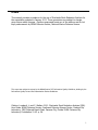
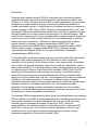
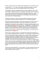
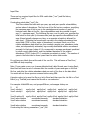
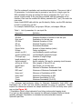
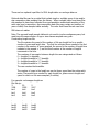
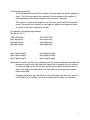
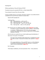
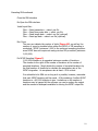
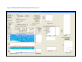
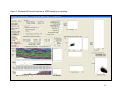
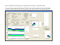
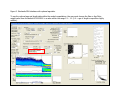
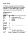
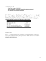
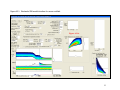
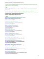
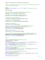
Stochastic
Stock Reduction Analysis
(SRA)
User Guide
1,3
Linda Lombardi
1
NOAA Fisheries Service
3500 Delwood Beach Road
Panama City, FL 32408
[email protected]
2,3
and Carl Walters
2
University of British Columbia
Fisheries Centre
British Columbia, Vancouver
[email protected]
3
University of Florida
Institute of Food and Agriculture Sciences
School of Forest Resources and Conservation
Fisheries and Aquatic Sciences Gainesville, FL 32653
Panama City Laboratory Contribution 2011-03
Preface
This manual provides procedures for the use of Stochastic Stock Reduction Analysis for
the executable produced in January 2011. These procedures are subject to change,
given future model changes. Opinions expressed herein are of the authors and do not
imply endorsement by NOAA Fisheries Service, National Marine Fisheries Service.
This report was subject to review by the NOAA Section 515 Information Quality Guidelines, abiding by the
Information Quality Act and Pre-Dissemination Review Guidelines.
Citation: Lombardi, L. and C. Walters. 2011. Stochastic Stock Reduction Analysis (SRA)
User Guide. NOAA Fisheries Service, Southeast Fisheries Science Center, Panama City
Laboratory, 3500 Delwood Beach Road, Panama City, Florida 32408. Panama City
Laboratory Contribution 11-03. p. 26.
1
Introduction
Stochastic stock reduction analysis (SRA) is a stochastic age structured population
model with Beverton-Holt stock-recruitment function that estimates forward in time
(Walters et al. 2006). SRA uses Umsy and MSY as leading parameters, and given these
parameters the model simulates changes in biomass by subtracting estimates of
mortality and adding recruits. A single trajectory of biomass over time is produced, as
well as, estimates of MSY, Umsy, U2009, Goodyear’s Compensation Ratio (recK), and
stock status. SRA is a less data-intensive method which can help to estimate how large
the stock needed to be to have produced the time series of observed landings. SRA
should not be a replacement for more computationally complex assessment models but
used more as a tool to make possible conclusions of stock status based on historical
catches and recent abundances. SRA has been applied to several Gulf of Mexico
species including red snapper (Lutjanus campechanus, SEDAR 2005), gag
(Mycteroperca microlepis, SEDAR 2006a), red grouper (Epinephelus morio, SEDAR
2006b), mutton snapper (Lutjanus analis, SEDAR 2008), yellowedge grouper
(Hyporthodus flavolimbatus, SEDAR 2011a), and golden tilefish (Lopholatilus
chamaeleonticeps, SEDAR 2011b).
In Stochastic SRA, recruitment is assumed to have had lognormally distributed annual
anomalies (with variance estimated from VPA estimates of recent recruitment
variability), and to account for the effects of these, a very large number of simulation
runs is made with anomaly sequences chosen from normal prior distributions (with or
without autocorrelation). The resulting trials of possible historical trajectories are used
as a starting point for Markov Chain Monte Carlo simulation (MCMC), but if the SIR
sampling is implemented more starting trials are necessary. During SIR sampling
regime SRA stores the priors and associated likelihoods, SIR only resamples within
these priors to find credible trials, and only a few probable best fit values are outputted
(bestfit.csv). Summing frequencies of occurrence of different values of leading
population parameter values over these sample amounts to solving the full state space
estimation problem for the leading parameters (i.e., find marginal probability
distribution for the leading population parameters integrated over the probability
distribution of historical state trajectories implied by recruitment process errors and by
the likelihood of observed population trend indices).
The stochastic SRA is parameterized by taking Umsy (annual exploitation rate producing
MSY at equilibrium) and MSY as leading parameters, then calculating the Beverton-Holt
stock-recruit parameters from these parameters and from per-recruit fished and
unfished eggs and vulnerable biomasses (Forrest et al. 2008). Under this
parameterization, we effectively assume a uniform Bayes prior for Umsy and MSY,
rather than a uniform prior for the stock-recruitment parameters. This is an agestructured version of the stock-recruitment parameterization in terms of policy
parameters suggested by Schnute and Kronlund (1996).
2
Natural mortality rate (M) is not treated as age-independent, and is determined from
M
survival rate (S = e- ). It is best to have fishery independent estimates of natural
mortality (if possible), given the size-selectivity practices of most fisheries.
Vulnerabilities at age can be calculated through a variety of methods (such as VPA,
dome-shaped or logistic selectivities). Age-specific vulnerabilities can vary by year to
track changes in historical fishing practices targeting specific age class or specific size
groups. Most fisheries have a high variance in abundances of older ages, thus
vulnerabilities can be fixed at an age when the vulnerabilities become stable (which
may or may not be the maximum age).
Fecundity is assumed to be proportional to the differences between age-specific
body weight and weight at maturity calculated from user-supplied parameters.
SRA provides probability distributions of leading parameters (Umsy, MSY) and other
population parameters (vulnerable biomass, catch, exploitation), as well as the
probability of the population being overfished or undergoing overfishing based on the
Pacific Fisheries Management Council 40/10 rule. The probability of overfishing shown
in the SRA interface (Figure 1) is calculated from the PFMC 40:10 rule whereby F is
targeted to be decremented below fishing mortality at maximum sustainable yield
(Fmsy) when the stock is less than 40% of virgin biomass, and F is targeted at zero
when the stock is less than or equal to 10% of virgin biomass. This rule is shown as
the diagonal line on Figure 1H.
SRA can also provide the proportion of overfished and overfishing as defined by the
given maximum sustainable yield as a benchmark. The probability of overfished occurs
when the spawning stock biomass in the last year of data/spawning stock biomass at
maximum sustainable yield (SSByear/SSBmsy) is less than one. The probability of
overfishing occurs when exploitation in the last year of data/exploitation at maximum
sustainable yield (Uyear/Umsy) is greater than one. SRA outputs a vector of
exploitation in the last year of data (Uyear)/exploitation at maximum sustainable yield
(Umsy) as well as a vector of spawning stock biomass in the last year of data (SSByear)
and a vector of spawning stock biomass at maximum sustainable yield (SSBmsy). The
user can calculate the proportion of SSByear/SSBmsy iterations that are less than one.
Each of these parameters is reported with a level of uncertainty determined through
MCMC.
SRA has three main assumptions: 1) the population is at virgin conditions the first year
data is provided, 2) there is stochastic variation in recruitment for all years, and 3)
survival rate is constant for all years.
3
Input Files
There are two required input files for SRA: catch data (".csv") and life history
parameters (".par")
Constructing catch data (".csv") file
This file contains the total catch per year, age and year specific vulnerabilities,
and an index of abundance. The first row of the file has two numbers, specifying
the maximum age of fish to use in the simulations and number of years of
historical catch data in the file. Age vulnerabilities must be provided for each
age (1 – maximum age). The following file rows, one for each year, specifies the
total catch for that year (in biomass units) and age-specific vulnerabilities for all
ages (these typically change over time, so a separate schedule is allowed for
each year). Following the annual catch records is the relative abundance time
series data (CPUE or other index of abundance) is entered. Each row of the
relative abundance data block has four numbers: sample year, abundance index
value, an independently estimated, log-normally distributed relative recruitment
anomaly for that year (value of 0.0 corresponds to average recruitment predicted
by stock-recruit relationship), and the standard deviation of the relative
abundance (CPUE) (value of 1.0, moderate uncertainty in index). The number of
years in the index can be fewer years than the entire catch series.
Do not leave any blank lines at the end of the .csv file. This will cause a ‘Run Error,’
and SRA will stop compiling.
Note: If you create a new .csv (comma delimited text) data file and save it using Excel,
then Excel will insert a set of commas after the number of years and ages on the first
file line, and after the relative abundance data on each of the lines in the data block.
You must edit out those spurious commas before using SRA.
A simpler option is to save the file as a .txt in Excel and then open the .txt file in a Text
Editor (e.g. TextPad) and resave the file with a .csv extension.
For example: tilefishSRA.csv; red grouperSRA.csv; red snapper history.csv
5
10
Year1 catchyr1
age1yr1vul age2yr1vul age3yr1vul age4yr1vul age5yr1vul
Year2 catchyr2
age1yr2vul age2yr2vul age3yr2vul age4yr2vul age5yr2vul
...
Year10 catchyr10 age1yr10vul age2yr10vul age3yr10vul age4yr10vul age5yr10vul
Year1 index relative
recruitment anomaly
standard deviation
Year2 index relative
recruitment anomaly
standard deviation
...
Year6 index relative
recruitment anomaly
standard deviation
Constructing life history parameters (".par") file
4
This file contains all population and recruitment parameters. There are a total of
20 parameters. A convenient way to generate a .par file is to simply open the
SRA executable file using an existing life history parameters file (“.par”) for a
species roughly similar to the one being modeled, edit the parameters in the
interface, then save the modified life history parameter file (".par") file under the
new name.
Users should NEVER edit with the .par file directly. Rather, use the SRA interface
to build or modify the .par file!
For example: tilefishSRA.par; red grouper SRA.par; red snapper SRA.par
Table 1. List of parameters for .par input file.
Parameter
Definition
Bhat year
Biomass in the last year, will reflect last year of data
SD Bhat
Standard Deviation of Number of fish last year
Uhat year**
Exploitation for the last year
SD Uhat
Standard Deviation of Uhat
SD rec
Standard Deviation of RecK
Rec rho
Recruitment Residuals
Future Catch
Amount of future landings (catch)
Ufuture
Future exploitation
growth von B K
von Bertalanffy growth coefficient
growth Linfinity (cm)
von Bertalanffy asymptotic length
CV length age
Variation of length at age
length maturity (cm)
Length at maturity
Age at maturity
Age at maturity; first age for spawning stock biomass
wt (kg) at 100 cm
Size (weight) of fish at 100 cm
growth tzero
Size (length, cm) at time zero
MSY min*
Minimum of Maximum Sustainable Yield
MSY max*
Maximum of Maximum Sustainable Yield
Umsy min*
Minimum of Exploitation at MSY
Umsy max*
S min
S max
Maximum of Exploitation at MSY
Minimum Survivalship (S-0.02)
Maximum Survivalship (S+0.02)
* The minimum and maximum values for Maximum Sustainable Yield (MSY) and
Exploitation (U) at MSY are best visually estimated as priors are compiled. Visually
inspect the relationship between the sample distribution of MSY and Umsy when priors
are run (see Figure 1A).
**Exploitation (Uhat) is best estimated from fishery independent tagging study.
If no such are data available, then examine the difference between total and natural
mortality estimates. Exploitation is calculated as catch/vulnerable biomass.
Optional Input Files
5
There are two optional input files for SRA: length data. csv and age data.csv
Optional data files can be provided that include single or multiple years of size and/or
age composition data sampled from the fishery. When included, data from these files
are assumed to have been collected from representative multinomial sampling of the
catch size (age) composition. Age composition data files may contain any number of
years of data, from samples taken annually. The order that these files are read into
SRA does not matter.
Note: The age and length sample tables do not need to involve contiguous years, but
must have the same number of age or size classes sampled every year.
Constructing length.csv file:
The file contains the count of the number of fish per length bin for a specific
number of years and length bins. The first line contains three numbers: the first
number is the number of years sampled, the second is the number of length bins
included in the sample + 1, and the third number is the number of lengths
increments in the bins.
The numbers of increments between length bins are categorized as follows:
0 = lengths 0 to binwidth
1 = lengths binwidth to 2 * binwidth
2 = lengths binwidth to 3 * binwidth
3 = lengths binwidth to 4 * binwidth
The user creates the binwidths.
The number of years in the length.csv can be fewer years than the entire catch
series. There must be a number for each length bin, place zeros in length and
years for which no fish were sampled (0 entries).
For example: red snapper length.csv
File Set-up:
3
50
2
1994
1995
2007
bin1
bin1
bin1
bin2
bin2
bin2
bin3
bin3
bin3
.
.
.
.
.
.
.
.
.
bin48
bin48
bin48
bin49
bin49
bin49
bin50
bin50
bin50
6
Constructing age.csv file:
The file contains the count of the number of fish per age for a specific number of
years. The first line contains two numbers: the first number is the number of
years sampled and the second number is the number of age bins.
The number of years in the length.csv can be fewer years than the entire catch
series. There must be a number for each age bin, place zeros in age and years
for which no fish were sampled (0 entries).
For example: red snapper age data.csv
File Set-up: 20 15
1984 1985
Age1 age1
Age2 age2
Age3 age3
1986 .
age1 .
age2 .
age3 .
.
.
.
Age13 age13 age13 .
Age14 age14 age14 .
Age15 age15 age15 .
.
.
...
...
...
...
2001 2002 2003
age1 age1 age1
age2 age2 age2
age3 age3 age3
age13 age13 age13
age14 age14 age14
age15 age15 age15
Remember to create .csv files: If you create a new .csv (comma delimited text) data file
and save it using Excel, then Excel will insert a set of commas after the number
of years and ages on the first file line, and after the relative abundance data on
each of the lines in the data block. You must edit out those spurious commas
before using SRA.
A simpler option is to save the file as a .txt in Excel and then open the .txt file in
a Text Editor (e.g. TextPad, Tinn-R) and resave the file with a .csv extension.
7
Figure 1. Stochastic SRA model interface.
Figure 1B
Figure 1A
Figure
1F
Figure 1G
Figure 1E
Figure 1C
Figure 1D
Figure 1H
8
Executing SRA
Platform specifications: Microsoft Windows 2003/XP
Download and save the executable SRA file to a folder labeled (SRA).
Copy and paste the input files in this same folder.
It does not matter where in your directory this folder is located, it only matters that the
executable and the input files are located in the same folder.
Open the SRA executable file
Install input files:
Files Read
Files Read
Files Read
Files Read
parameters select .par file
time series data select .csv file
length data select .csv file (optional)
age data select .csv file (optional)
Run Priors The user can indicate the number of trials (Figure 1B), as well as,
the number of years to simulate before either the MCMC or SIR sampling
is conducted. MCMC (minimum 1,000) is the preferred sampling
procedure since MCMC does not require as many priors as SIR procedure
(minimum 1,000,000).
After the trails are compiled, the user should visually inspect the distribution of
data shown in the plots on the interface.
If the plot of the vulnerable biomass trajectories is not displayed correctly,
than either increase or decrease the biomass scaler (default 0.5, Figure
1C).
If the sample distribution of Umsy and MSY values is not fully distributed
throughout the designated area, than either decrease or increase the
range of these two parameters (Figure 2A).
Run Priors again
If the display is satisfactory, than save parameters: Files Save parameters
9
Executing SRA continued
Close the SRA interface
Re-Open the SRA interface
Install input files:
Files Read
Files Read
Files Read
Files Read
parameters select .par file
time series data select .csv file
length data select .csv file (optional)
age data select .csv file (optional)
Run Priors
The user can indicate the number of trials (Figure 1B), as well as, the
number of years to simulate before either the MCMC or SIR sampling is
conducted. MCMC (minimum 1,000) is the preferred sampling procedure
since MCMC does not require as many priors as SIR procedure (minimum
1,000,000).
Do MCMC Sampling (Figure 3)
1,000,000 iterations is a suggested minimum number of iterations
The number to the right of the number of iterations is the number of
accepted iterations. Simply divide the number of accepted iterations by
the total number of iterations to calculate the acceptance rate of the
MCMC integration. An acceptance rate at least ~30% is ideal.
It is advisable to let SRA run as long as it is possible, however, remember
that each MCMC iterations will be saved. A file containing 2 million MCMC
iterations is ~400,000 kilobytes in size. Limitations on the number of
iterations may be caused by the software you use to analyze the output
and the amount of diskspace available for storing the MCMC output file.
10
Figure 2. Stochastic SRA model interface after Priors are run.
Figure 2A
11
Figure 3. Stochastic SRA model interface as MCMC sampling is executing.
Figure 3A
12
Figure 4. Stochastic SRA model interface once MCMC iterations are manually or automatically stopped.
To save the interface, enlarge the SRA interface, CTRL-Print Screen, and Paste into Microsoft Powerpoint/Word/Ecel.
Remember to also save the output files in a separate folder (a new compile of SRA will overwrite these output files).
13
Figure 5. Stochastic SRA interface with optional age data.
To use the optional age and length data within the model computations, the user must change the Size or Age Distn
weight value from the default 0.00000001 to a value within the range 0.1 – 1.0 (1.0 = age or length composition highly
reliable).
14
Markov Chain Monte Carlo simulation (MCMC)
SRA uses MCMC with a Metropolis-Hastings random walk algorithm to resample possible
historical stock trajectories by summing frequencies of occurrence of different values of
leading population parameter values over these sample amounts to solve the full state
space estimation problem for the leading parameters (i.e. find marginal probability
distribution for the leading population parameters integrated over the probability
distribution of historical state trajectories implied by recruitment process errors and by
the likelihood of observed population trend indices). MCMC convergence is usually
most rapid when the acceptance rate is around 20%; this is not a mathematical
requirement, but a practical one since very low acceptance rates (< 5%) typically mean
very slow sampling of the parameter space, i.e. requirement for many millions of trials
to adequately sample the space. Very high acceptance rates likewise usually mean that
the sampler is moving too slowly over the space, accepting too many tiny moves.
There are two parameters (Par step and Anom Step, Figure 1F) in SRA to bound the
maximum sizes of random parameter changes tested by the MCMC sampling procedure.
These have to be adjusted manually in cases where the acceptance rate is too high or
low. Setting lower steps typically causes higher acceptance rates, but slower movement
over the parameter space (watch the sample trial Umsy, MSY combinations sampled
over trials as the MCMC proceeds).
Currently, SRA does not include more sophisticated MCMC routines such as multiple
sample chains or tests for convergence as sample size increases. Absent of such
methods, allow the model to run very, very long runs (e.g. 8hr, ~5,000,000,000 trials)
to obtain convergence of any Bayes posterior sampling methods and compare how the
long against shorter runs (~1,000,000 trials). (The speed of a run is dependent upon
the processor of your computer, the computer's bus speed, and the speed of disk
operations.)
The number of trials completed, as well as, the number of trials accepted are shown on
the interface (Figure 3A: number of trials (right), number of acceptable trials (left)).
15
Output Files
SRA provides four output files:
1.
Pop.csv
A grid of MCMC sample frequencies for biomass over time (biomass grid points in
columns, relative frequencies of occurrence in rows).
2.
Par.csv
The MCMC sampled estimates of maximum sustainable yield (MSY), exploitation
at MSY (Umsy), survival rate (S), egg production for the final year of data/egg
production in the virgin year (E year/Eo), exploitation for the final year of
data/exploitation at MSY (U year/Umsy),Goodyear’s recruitment compensation
ratio (RecK), biomass total in final year of data (Btot 2009), spawning stock
biomass for the final year of data (SSB 2009), and spawning stock biomass at
maximum sustainable yield (SSBmsy). The output does not contain the first 200
MCMC burn-in iterations. This data is not automatically plotted. R code is
provided for basic plots of MSY, Umsy, S, Ucurrent, RecK, and stock status (see
Appendix 2). The Par.csv file contains multiple duplicate rows and rows of unique
values. The total number of trials equals the total number of rows. The
number of unique rows equals the number of accepted trials.
3.
PopandU.csv
The best population (pop) estimates and exploitation (u) estimates for each year,
estimated as the mean values of the sampled biomass and exploitation
combinations during the MCMC (these modes do not necessarily correspond to
any single trajectory sampled during the MCMC trials; that trajectory is in
bestfit.csv). This data is not automatically plotted. Note: The population
estimates shown in this file need to be scaled to the biomass scaler value as
indicated on the interface. The ‘true’ values of the population estimates need to
be multiplied by the biomass scaler.
4.
bestfit.csv
The estimates of vulnerable biomass, observed catch, and exploitation (U) by
year for the most likely parameter combination found during SIR procedure.
This file is only created when SIR sampling is compiled. The user must indicate
the number of priors to be compiled by the SIR posterior sampling. It is advised
that the number of priors is a minimum of 1,000,000.
These output files will be created as the MCMC sampling is begun and will write over
any previous model compilation output files. If you wish to save a model’s output, than
copy and paste these files in another folder before SRA is executed.
16
Problem Solving and Further Guidelines (in alphabetic order)
Age Vulnerabilities: Considering the high variance in abundances of older ages, fix the
vulnerabilities at age not at the maximum age but at an age the
vulnerabilities level off. For example, for red grouper maximum age
30, vulnerabilities were fixed at age 17.
Exploitation (Current): U current = Umsy* U year/Umsy Umsy and Uyear/Umsy refer to
the column headings in the Par.csv output file.
NPV: Mean NPV (see Figure 1G) is an index of economic performance for forward
simulations from the end of the historical data. It is the discounted sum of future
catches over the simulation period, averaged over simulation trials. It only has
meaning when you are comparing alternative future TAC or U policies.
RecK: Good year's Recruitment Compensation Ratio (recK) is calculated from estimates
of Umsy and MSY values, and SRA’s sampler will only except positive integers for
recK. Any combinations of Umsy and MSY that yield a negative recK are ignored.
Refer to the Compensation ratio plot (see Figure 1D) at the bottom of the
interface for the distribution of calculated recK values.
Run Error: SRA will occasionally stop and a ‘Run Error’ window will appear.
Possibly causes for this error:
1. Incorrect set up of .csv file (no blank lines are allowed, check end of file).
2. MCMC sampling is experiencing trouble sampling along a narrow ridge of
parameter combinations (re-evaluate population parameters, variation in
index, standard deviation of recruitment, etc.). Suggest opening Par.csv
from the crashed model run to view parameter values, normally in this kind
of error there is no change in MSY, Umsy, S, E year/Eo, U year/Umsy and
RecKs are mostly negative.
Survival rate: Survival rate S is S = exp (-M). A general observation (from Pauly’s
meta-analysis of natural mortality, M) is that M should be between 1.1 *
von B K and 1.6 * von B K, where K is the von Bertalanffy metabolic
parameter. But another estimator of M would be the Hewitt-Hoenig
estimate from maximum age (M = 4.3/max age). Considering setting the
S range depending on the uncertainty in the natural morality estimate for
your species modeled.
Variance in Index of Abundance: Labeled “var of abundance index” on the SRA
interface is defaulted to 0.04 (Figure 1E). This is the assumed
observation variance of the log relative to the index of abundance
(e.g. log CPUE) corresponding to catchability * biomass mean
value for each year. The default value represents a standard
17
deviation (CV on arithmetic scale) of around 0.2, a typical for
relative abundance time series. Using higher variance values:
Increasing the variance does not only assume the CPUE is ‘noisy’
but has another effect, namely to spread out the likelihood
function so that the MCMC has higher acceptance rates, allowing it
to move over the parameter space more widely and thus find the
ridge of high probability combinations for U 2009/Umsy and E
year/Eo.
Weight at 100cm: Although your species may not reach this size, this weight provides
any easy way to parameterize the length weight relationship.
18
Literature Cited
Forrest, R., Martell, S., Melnychuk, and C. Walters. 2008. Age-structured model with
leading management parameters, incorporating age-specific selectivity and maturity.
Can. J. Fish. Aquat. Sci. 65: 286-296.
Schnute, J.T. and A.R. Kronlund. 1996. A management oriented approach to stock
recruitment analysis. Can. J. Fish. Aquat. Sci. 53:1281-1293.
Southeast Data, Assessment and Review (SEDAR). 2005. Stock Assessment Report of
SEDAR07, Gulf of Mexico Red Snapper. Report 1. SEDAR, One Southpark Circle #306,
Charleston, SC 29414
SEDAR. 2006a. Stock Assessment Report of SEDAR10, Gulf of Mexico Gag Grouper.
Report 2. SEDAR, One Southpark Circle #306, Charleston, SC 29414
SEDAR. 2006b. Stock Assessment Report of SEDAR12, Gulf of Mexico Red Grouper.
Report 1. SEDAR, One Southpark Circle #306, Charleston, SC 29414
SEDAR. 2008. SEDAR 15A. Stock Assessment Report 3 (SAR 3) of South Atlantic
and Gulf of Mexico Mutton Snapper. One Southpark Circle #306, Charleston, SC
29414
SEDAR. 2011a. Stock Assessment Report of SEDAR 22, Gulf of Mexico Yellowedge
Grouper. Report 1. SEDAR, One Southpark Circle #306, Charleston, SC 29414
SEDAR. 2011b. Stock Assessment Report of SEDAR 22, Gulf of Mexico Golden Tilefish.
Report 1. SEDAR, One Southpark Circle #306, Charleston, SC 29414
Walters, C.J., S.J.D. Martell, and J. Korman. 2006. A stochastic approach to stock
reduction analysis. Can. J. Fish. Aquat. Sci. 63: 212-223.
19
Appendix 1.
Editing par.csv file for use in R.
The header of the par.csv file needs a few edits before used in the following R files.
Original header:
MCMC MSY,Umsy,S,E 2009/Eo,U 2009/Umsy,RecK,Btot 2009,SSB 2009,SSBmsy
Need to remove the following:
MCMC
Space between E 2009
Space between U 2009
Space between Btot 2009
Space between SSB 2009
Edited header:
MSY,Umsy,S,E2009/Eo,U2009/Umsy,RecK,Btot2009,SSB2009,SSBmsy
20
Appendix 2: Model Example
In March 2011, SRA was presented at the Assessment Tools Workshop (Oregon State
University, Portland, Oregon). This workshop’s focus was simple stock assessment
models for data-poor species. Several models were discussed and SRA was applied to
one of the 50 data-poor stocks managed in the Pacific Coast Groundfish Fishery, the
aurora rockfish (Sebastes aurora). SRA results were compared to model runs from
Depletion-Based Stock Reduction Analysis (DB-SRA, Dick and MacCall 2010) and Simple
Stock Synthesis (SSS, J. Cope, pers. comm.. NWFSC, Seattle, WA). DB-SRA and SSS
are based on 4 main data inputs: 1) natural mortality (M), 2) ratio of Fmsy/M, 3) ratio
of Bmsy/K (K = carrying capacity), and 4) relative stock status. SSS also requires
weight-length relationships as well as dimensioning of the length and age bins. The
comparisons of these three models provide an example of using limited data input
through a variety of model compilations. Resulting Overfishing Levels (OFLs) were
similar among models (Table A2.1).
SRA model inputs
Constructing .par file
Parameter
Value
Bhat year
500
SD Bhat
Uhat year
SD Uhat
SD rec
Rec rho
Future Catch
Ufuture
growth von B K
growth Linfinity
(cm)
CV length age
length maturity
(cm)
Age at maturity
wt (kg) at 100 cm
growth tzero
3000
0.03
0.05
0.5
0
0
0.1
0.12
37
0.10
17
Comment
Initial value calculated using average historical catch (29
mt) divided by exploitation = 0.05
Assumed large uncertainty in biomass
The initial value for Uhat was 0.03 with SD Uhat 0.02.
SD Uhat was increased to 0.05 for final model runs.
Default value
Default value
Based on minimal future exploitation
Values, except for wt (kg) at 100 cm and CV length
at age, reported in Dick and MacCall 2010.
5
11.26
0
MSY range
0 - 100
Umsy range
0.01-0.12
S range
0.92-0.96
Range of MSY was manipulated until distribution of MSY
was normally distributed (Figure A2.1A).
The initial values of Umsy were set at Fmsy = 0.05.
Range of Umsy was manipulated until distribution of Umsy
was normally distributed (Figure A2.1A).
M = 0.06 (maximum age 75 yr) (Dick and MacCall 2010)
21
Constructing .csv file
Catch (mt) by year: 1916-2009
Age vulnerabilities: knife edge vulnerabilities beginning at age 5
No Index and No recruitment anomalies
Table A2.1. Comparison of Overfishing Limits (OFLs) among three assessment models:
Stochastic Stock Reduction (SRA), Depletion-Based Stock Reduction Analysis (DB-SRA,
Dick and MacCall 2010) and Simple Stock Synthesis (SSS, J. Cope, pers. comm..
NWFSC, Seattle, WA). *Overfishing limits in SRA were calculated by multiplying the
predicted vulnerable biomass in the last year of data by Umsy.
Model
SRA Uhat 0.03 ± 0.02
SRA Uhat 0.03 ± 0.50
DB – SRA
SSS with symmetric depletion prior
SSS with informed beta depletion prior
OFLs in 2010
55*
43*
47 (median)
56 (median)
66 (median)
Literature Cited
Dick, E. J. and A. D. MacCall. 2010. Estimates of sustainable yield for 50 data-poor
stocks in the Pacific Coast Fishery Management Plan. NOAA Technical Memorandum.
NOAA-TM-NMFS-SWFSC-460.
22
Figure A2.1. Stochastic SRA model interface for aurora rockfish.
Figure A2.1A
23
Appendix 3. Summary of SRA output parameters (par.cvs)
# Purpose: provides parameter summaries from output of Stochastic Stock Reduction Analysis (SRA)
# Data file: Par.csv ouput file from SRA
# Data
output = unique(read.table("Par.csv", sep = ",", header = T)) #only unique rows used for analysis
attach (output)
output2 = subset(output, output$RecK >0) #removes negative recK values from dataframe
output3 = subset(output2, output2$RecK <101) #removes larger than 101 recK values from dataframe
biomassbenchmark = output2$SSB2009/output2$SSBmsy
Ucurrent = output2$Umsy*output2$U2009.Umsy
# Output
print("Summary Yellowedge Grouper WEST GOM: CMLL Index")
print("Estimates of Maximum sustainable yield")
print(mean(output2$MSY)); print(sd(output2$MSY))
print(summary(output2$MSY))
print("Estimates of Exploitation at MSY")
print(mean(output2$Umsy)); print(sd(output2$Umsy))
print(summary(output2$Umsy))
print("Estimates of Current Exploitation")
print(mean(Ucurrent)); print(sd(Ucurrent))
print(summary(Ucurrent))
print ("Summary recK")
print("recK: all positive values")
print(mean(output2$RecK)); print(sd(output2$RecK))
print(summary(output2$RecK))
print("recK: all values between 1 and 100")
print(mean(output3$RecK)); print(sd(output3$RecK))
print(summary(output3$RecK))
print ("Summary Total Biomass last year")
print(mean(output2$Btot2009)); print(sd(output2$Btot2009))
print(summary(output2$Btot2009))
print ("Summary Spawning Stock Biomass last year")
print(mean(output2$SSB2009)); print(sd(output2$SSB2009))
print(summary(output2$SSB2009))
print ("Summary Spawning Stock Biomass at MSY")
print(mean(output2$SSBmsy)); print(sd(output2$SSBmsy))
print(summary(output2$SSBmsy))
print ("Summary SSBcurrent/SSBmsy")
print(mean(biomassbenchmark)); print(sd(biomassbenchmark))
print(summary(biomassbenchmark))
print ("Summary Ucurrent/Umsy")
print(mean(output2$U2009.Umsy)); print(sd(output2$U2009.Umsy))
print(summary(output2$U2009.Umsy))
24
Appendix 4. Plotting parameters of SRA output and Stock Status Figure
# Purpose: plot simulated estimates of MSY, Umsy, recK, Ucurrent, and stock status from output of SRA
# Data file: Par.csv ouput file from SRA
# Data
outputalldata = unique(read.table("Par.csv", sep = ",", header = T)) #only unique rows used for
analysis
attach (outputalldata)
#Restricts the dataset to only sample combinations resulting in a postive recK
outputalldata2 = subset(outputalldata, outputalldata$RecK >0)
#Restricts the dataset to only sample combinations recK 1-100
outputalldata3 = subset(outputalldata2, outputalldata2$RecK <101)
#Calculating esimates of current exploitation
Ucurrentalldata = outputalldata2$Umsy*outputalldata2$U2009.Umsy
#Calculate the ratios of SSBcurrentyr/SSBmsy
biomassbenchmark = outputalldata2$SSB2009/outputalldata2$SSBmsy
#Provides the number of ratios
nbiobenchmark = length(biomassbenchmark)
#Proportion Overfished, provides the number of biomass benchmarks are less than one
noverfished = length (subset(biomassbenchmark, biomassbenchmark < 1.0))
percentoverfished = (noverfished/nbiobenchmark)*100
print("Proportion Overfished"); print(percentoverfished)
#Provides the number of ratios
nexploitbenchmark = length(outputalldata2$U2009.Umsy)
#Proportion Overfishing, provides the number of exploitation benchmarks are greater than one
noverfishing = length (subset(outputalldata2$U2009.Umsy, outputalldata2$U2009.Umsy > 1.0))
percentoverfishing = (noverfishing/nexploitbenchmark)*100
print("Proportion Overfishing"); print(percentoverfishing)
# Graphs
# Graph, x and y limits may need to be adjusted given your data
x11(width=80, height=50, pointsize=8)
par (mfrow=c(2,1))
utils::str(hist(outputalldata2$MSY, xlim = c(30000, 100000), ylim = c(0, 150000),breaks = 30, col=
"green3", labels = TRUE, xlab = "Maximum Sustainable Yield"))
utils::str(hist(outputalldata2$Umsy, xlim = c(0.05,0.20), ylim = c(0, 150000),breaks = 25, col=
"darkorange", labels = TRUE, xlab = "Exploitation at MSY"))
# Graph, x and y limits may need to be adjusted given your data
x11(width=20, height=5, pointsize=8)
utils::str(hist(outputalldata3$RecK, xlim = c(0, 100), ylim = c(0, 300000), breaks = 25, col="blue2",
labels = TRUE, xlab = "Goodyear's Compensation ratio"))
# Graph, x and y limits may need to be adjusted given your data
x11(width=80, height=50, pointsize=8)
utils::str(hist(Ucurrentalldata, xlim = c(0.001,0.20), ylim = c(0, 250000),breaks = 25, col="lightblue3",
labels = TRUE, xlab = "Current Exploitation"))
x11(width=80, height=50, pointsize=8)
25
#Smooth Scatter color symbolizes density of points (red highest density).
smoothScatter(biomassbenchmark, outputalldata2$U2009.Umsy, colramp = colorRampPalette(c("white",
"blue", "green", "yellow", "orange", "red")), nrpoints = 0,
xlim = c(0.0,3.0), ylim = c(0.0,3.0), xlab = "SSBcurrent/SSBmsy", ylab = "Ucurrent/Umsy", main =
"Stock Status")
abline(h=1, col = "red")
abline(v = 1, col = "red")
text (0.2, 2.5, "Overfished and ", font=2)
text(0.2, 2.4, "Overfishing", font = 2)
text (0.1,0.1,"Overfished", font = 2)
text (2.0,2.5,"Overfishing", font = 2)
26