
1
ZINC Tutorial Manual
Introduction ................................................................................................................................ 1
Example 1: Dielectric Problem .................................................................................................. 2
Introduction ............................................................................................................................ 2
Geometry and meshing........................................................................................................... 5
Input file *.zin ...................................................................................................................... 13
Running the simulation ........................................................................................................ 14
Viewing the output. .............................................................................................................. 16
A quick look at the result ..................................................................................................... 17
Post processing..................................................................................................................... 18
Traceability........................................................................................................................... 24
More advanced graph plotting.............................................................................................. 24
If you don’t like gnuplot....................................................................................................... 31
Also in the directory............................................................................................................. 31
Example 2: piezoelectric example............................................................................................ 31
Introduction .......................................................................................................................... 31
Simulation ............................................................................................................................ 34
Results .................................................................................................................................. 37
Comparison graphs............................................................................................................... 42
Also in the directory............................................................................................................. 43
Example 3: Fuel cell................................................................................................................. 43
Introduction .......................................................................................................................... 43
Zinc implementation ............................................................................................................ 48
DLL method ......................................................................................................................... 49
Expressions method.............................................................................................................. 53
Running the simulation ........................................................................................................ 54
Also in the directory............................................................................................................. 60
Appendix A: Description of differential equations .................................................................. 60
Introduction
This tutorial manual shows a series of real life problems being solved with Zinc. It is probably
the best place to learn how to use the program, though it may be helpful to refer back to the
User Manual from time to time. Each tutorial corresponds to one of the examples in the
“examples” folder that came with your Zinc distribution. These folders contain the input and
output files for the simulation as generated by us. When you run the simulations, you should
check you get the same answers we did. It’s probably a good idea to copy the input files to a
fresh folder so as not the overwrite the output files we’ve supplied. That way, you can do a
comparison easily.
1
Example 1: Dielectric Problem
Directory: examples/dielectric
Introduction
ZINC is a finite element program that is designed to solve problems having the form
− ∇ . ( C ∇U ) + a U = f ,
(1)
which is written explicitly in component form as follows
−
∂
∂xi
αβ ∂U β
C ij
+ a αβ U β = f α , α = 1, 2, ... , N
∂
x
j
(2)
where summation over 1, 2, …. N (where N is the number of variables) is implied by repeated
Greek superscripts, and where summation over 1, 2, 3 is implied by Arabic suffices.
Appendix A gives a more detailed description of the notation and definitions. The reader can
also refer to the Zinc User Manual, Chapter 4, for a more detailed description.
In this tutorial, the problem is to determine the electrical potential distribution, and other
derived properties such as the electric field and displacement field. The system consists of a
spherical sample of one type of material that is embedded in a cuboid of another material. The
system is excited by a potential difference between opposing faces of the cuboid. This
problem is in fact mathematically equivalent to both thermal and electrical conduction
problems, and to diffusion and magnetic permeability problems.
The field equations that must be solved is one of Maxwell’s equations, in the absence of
distributed charge, namely,
∇. D = 0 ,
(3)
where D is the electric displacement whose value is given by the constitutive relation
D = ε ε0E ,
(4)
where E is the electric field, ε0 is the permittivity of free space and ε is the relative
permittivity (a dimensionless material property). The electric field is related to the electric
potential V according to the relation
E = − ∇V .
(5)
The relations (3)-(5) imply that the electric potential must satisfy the equation
− ∇. ( ε ε0∇V ) = 0 .
2
(6)
In component form this equation is written
(
), j = 0 .
− ε ε 0 V, j
(7)
The relation (7) results from (2) if the following identifications are made (See Zinc User
Manual, Chapter 4)
N = 1,
a11 = 0,
f 1 = 0,
U1 = V,
C11
ij = ε ε0 δij ,
(8)
where δij is the Kronecker delta symbol having the value 1 if i = j, 0 otherwise. It follows
from (A10) that the C matrix used by ZINC has the values given by
11
C 1i1 j = C ij = εε 0δ ij
(9)
It should be noted that in ZINC all coefficients appearing in the general differential equations
(2) are zero unless non-zero values are set in the ZINC input files *.zin where * denotes an
input filename introduced by the user.
The differential equation (7) has a unique solution only if suitable boundary conditions are
applied.
The boundary condition assumed by Zinc is
∂U β
+ q αβ U = g α
∂x j
where n is the unit normal on the surface. It is easy to check that with
αβ
ni C ij
q11 = g 1 = 0
this becomes
n⋅D = 0
or
∂V
=0
∂n
which is the usual open boundary condition used in electrical problems. It implies the electric
field, E, will be parallel to the outer edges of the simulation. In the example to be solved this
boundary condition applies everywhere on the external surface of the system except on two
opposing planes of the cuboid where differing uniform electric potentials are to be imposed.
These Dirichlet boundary conditions are imposed simply be fixed the values of the nodes at
the appropriate potential (which will be simply 1 V and 0V). In ZINC, any unset components
of the C, a, f, q, g matrices defaults to zero so the condition n ⋅ D = 0 occurs automatically.
At the surface of the spherical region the normal component of the electric displacement must
be continuous across the boundary, and the electric potential must also be continuous across
this boundary. Provided we leave q and g at their default zero values, this condition will also
occur automatically. The boundary conditions that apply are illustrated in Fig.1.
3
Fig.1: Schematic diagram of geometry and the boundary conditions.
The default condition on the external boundary of Region 1 is, therefore,
∂ V1
=0,
∂n
implying that
n.D = 0 ,
(10)
where n is the unit outward normal to the free surface.
On the plane z = 1
On the plane z = −1
V1 = 1 ,
(11)
V1 = 0 .
(12)
On the interface between Regions 1 and 2 the following conditions must be satisfied
V1 = V2 , ε1
∂ V1
∂ V2
= ε2
,
∂n
∂n
implying that n . D is continuous across the interface, (13)
where n is now the unit outward normal to the interface, ∂ / ∂ n denotes the normal derivative
and where εi is the relative permittivity of Region i. The conditions (13) ensure that the
normal component of the electric displacement vector and the tangential component of the
electric potential are continuous across the surface. These “continuity conditions” are true, by
default, for all such internal interfaces and normally the user only needs to think about
applying boundary conditions at the outer surfaces.
4
The other boundary condition is the Dirichlet boundary in which the unknown variables, U,
are set at fixed values. In this tutorial, we will use the Dirichlet boundary at the top and
bottom faces of Fig 1 and the Neumann condition (n.D=0) at all other faces.
Geometry and meshing
Having installed ZINC onto your computer, it is useful to generate a new folder having name
‘ZINC_Runs’ (or similar) into which all simulations will be generated and saved. To deal
with the first example of this tutorial a new folder within ‘ZINC_Runs’ is created having the
filename ‘Dielectric’. This file will now be denoted in the following text by ‘*’.
Input file *.min
To represent the geometry shown in Fig.1 by finite elements the following input file must be
written and stored in ZINC_Runs/Dielectric. The first step defines the global mesh of cubic
elements which represents the entire region of the problem. The remainder of the file defines
‘parts’ of the system that are needed to define homogeneous regions having specific
properties and boundary and interface conditions. In the following code comments are
included to provide some explanation. More details of the *.min file are given in the Zinc
User Manual.
global
format ascii
xmesh
-1 1 0.2
end
The x range -1 < x < 1 is divided into elements of length 0.2
ymesh
-1 1 0.2
end
The y range -1 < x < 1 is divided into elements of length 0.2
zmesh
-1 1 0.2
end
The z range -1 < x < 1 is divided into elements of length 0.2
end
part 1
region 1
type box
fab 2 2 2
end
Defines a cubic box having sides of length 2 as Region 1
part 2
Defines a sphere having
region 2
type sphere
fab 0.5
surface region 1
end
part 3
radius 0.5 as Region 2, inserted into Region 1
Defines Region 3 to be the upper plane (z = 1)
5
region 3
type boundzup
end
part 4
region 4
type boundzdn
end
Defines Region 4 to be the lower plane (z = −1)
endfile
The next step is to generate a mesh using zmesh.exe which appears as two windows shown in
Figs. 2 and 3. The ZMesh window (Fig.2) enables the user to generate the required mesh
while the Output window (Fig.3) provides information on locations of files being used.
Fig.2: Window first opened by Zmesh.
6
Fig.3: Output window first opened by Zmesh.
Select File > Open MIN and open the file *.min whose contents are then displayed (see
Fig.4).
Fig.4: Window opened by Select File > Open MIN showing file *.min.
Select File/Process to generate the mesh. Provided no error occurred, the resulting mesh is
shown on screen and the mesh file is automatically stored as *.mtf in the folder ‘*’. The main
window now shows the geometry and mesh that has been generated (Fig 5). To view the
geometry from different angles, drag with the mouse.
7
Fig.5: Window opened by Select File > Open MIN showing file *.min after rotation of model.
Dragging rotates the model so that its 3D nature can be observed. It can be returned to a
standard state simply by pressing the buttons x, y or z which shows the view along the
selected axis.
NOTE:
Can rotate by dragging with mouse, or use arrow keys. Hold down SHIFT while dragging
with mouse to shift (rather than rotate) the figure. Press keys A/Z to zoom in/out and N/M to
rotate in the plane.
To observe the sphere alone press the button ‘Elem 1’ (in the key at the right) which switches
off the elements in Region 1 and reveals the embedded sphere in Region 2 (see Fig.6). When
the elements of a region are switched off a cross appears in the key symbol. Click on the key
symbol again to toggle the elements back on.
8
Fig.6: Spherical region is exposed by switching off the elements of Region 1.
The elements of Region 2 can be switched off by pressing the button ‘Elem 2’ and so on.
Nodes can also be toggled on or off by clicking on the key symbols marked ‘node 1’ etc. The
geometry of the nodes is best seen by dragging. Repeated pressing of all buttons simply
toggles between two possible states; visible or invisible. In Fig.7 is shown the result of
retaining the elements of Region 2 but showing the nodes.
Fig.7: Elements and nodes of spherical region shown by a suitable choice of active buttons.
9
The colours of the nodes and elements can be changed by right-clicking on node or element
buttons on top right hand side of the window. The colour is selected by specifying the mix of
primary colours using the Set Colour dialogue box (see Fig.8). The result of changing node
colours is shown in Fig. 9 while the result of changing element colours is shown in Fig.10.
Fig.8: Dialogue box for selecting the colours of elements and nodes.
Pressing the ‘xslice’, ‘yslice’ or ‘zslice’ buttons shows only a slice of the model in the x, y, or
z directions. The location of the slice can be changed using the Up/Down arrows on the
keyboard. While doing this, you can continue to rotate the system by dragging or use keys
A/Z or N/M normally. An example is shown in Fig.11 where the slice intersects both Regions
1 and 2. The elements for Region 2 can be switched off in a slice as shown in Fig.12.
10
Fig.9: The result of changing the colours of the nodes of the spherical region.
Fig.10: The result of changing the colours of the elements of the spherical region.
11
Fig.11: Example of a slice through Regions 1 and 2.
Fig.12: Example of a slice through Region 1 where elements for Region 2 are switched off.
In this case, the mtf file that is generated by Zmesh.exe is:
12
IMax:
JMax:
KMax:
10
10
10
I
J
K
x
y
z
RegNo RegUp
========================================================================
0
0
0 -1.0000E+00 -1.0000E+00 -1.0000E+00
4
1
1
0
0 -7.9998E-01 -1.0000E+00 -1.0000E+00
4
1
2
0
0 -5.9995E-01 -1.0000E+00 -1.0000E+00
4
1
3
0
0 -3.9991E-01 -1.0000E+00 -1.0000E+00
4
1
4
0
0 -1.9992E-01 -1.0000E+00 -1.0000E+00
4
1
5
0
0 2.2495E-05 -1.0000E+00 -1.0000E+00
4
1
6
0
0 1.9996E-01 -1.0000E+00 -1.0000E+00
4
1
7
0
0 3.9992E-01 -1.0000E+00 -1.0000E+00
4
1
8
0
0 5.9993E-01 -1.0000E+00 -1.0000E+00
4
1
9
0
0 7.9996E-01 -1.0000E+00 -1.0000E+00
4
1
10
0
0 1.0000E+00 -1.0000E+00 -1.0000E+00
4
0
0
1
0 -1.0000E+00 -7.9998E-01 -1.0000E+00
4
1
Etc. …………
The MTF file is not mysterious, it is just a text file showing the locations of nodes, their
Region, and their connectivity to neighbouring regions. This file is read in by the program
Zincwin (see later). Normally, the user does not have to look at this file.
Input file *.zin
ZINC requires information that controls the performance of the software, materials data for
each region, and data relating to boundary conditions that are not set by default. For the
dielectric problem this information is given in the following *.zin file:
! = 1 for static or steady/cyclic states, = 2 for transient problems
! No. of unknown variables (in this case just one: electrostatic potential)
! No. of iterations
! Successive over-relaxation parameter (<1) (Default 0.1)
! No. of Regions in model
! = 0 start from initial condition in *.zin (=1 continue from previous sim.)
! scaling factor for lengths found in *.mtf
! List of unknown variables (nvar in number)
key_sim=1
nvar=1
nstep=10000
omega=0.1
nreg=4
key_rdu=0
scale=1
labels=V
region 1 elements 3 values C
1 1 1 1 =
1 2 1 2 =
1 3 1 3 =
eps1
eps1
eps1
region 2 elements 3 values C
1 1 1 1 =
1 2 1 2 =
1 3 1 3 =
!For elements of Region 1 the are 3 non-zero
!coefficients of ZINC matrix C
!For elements of Region 2 the are 3 non-zero
!coefficients of ZINC matrix C
eps2
eps2
eps2
region 3 nodes 1 values
1 = 1.0
!For nodes of Region 3 there is 1 value 1.0 for unknown variable
13
region 4 nodes 1 values
1 = 0.0
!For nodes of Region 4 there is 1 value 0.0 for unknown variable
Init
1 = 0.0
!Initial value 0.0 for unknown variable
In this problem, as specified in Eq (8), the C matrix coefficients are just the permittivities. In
this simple case, all regions are isotropic so permittivities 11=22=33. Note that coefficient
1111 is permittivity 11; 1212 is permittivity 22 etc. The first and third index numbers refer to
the variable while the second and forth relate to spatial dimension (See User Manual, Chapter
4). In this case, there is only one variable so all indexes are 1x1y. It would, of course, be easy
to simulate an anisotropic dielectric rather than an isotropic one as in this example.
The constants “eps1” and “eps2” are in the constants file, dielectric.con. They specify the
permittivity of both regions. You can easily change these permittivities without altering the
dielectric.zin file.
Running the simulation
Having prepared the Zinc input file, it is time to run the actual simulation using Zinc shown in
Fig 13. Zinc also pops up an additional console window. As Zinc runs, information about
convergence is written into the console window.
Fig 13: Zinc (core) window
Now, use the Open button to select the file dielectric.zin, Fig 14
14
Fig 14: Zinc window with “dielectric.zin” selected.
The program checks all input files are present and shows the filename of
each. To run Zinc, at least an input file (*.zin) and a mesh file (*.mtf)
are needed. The constants and non-linearity (NL) files are optional. A
restart file is needed only in the case key_rdu=1 (which means, “continue
where you left off”. Since we’ve set this to zero (see above), this is not
needed.
You can view any file but clicking on the “view” button next to it. In Fig
15, we are viewing the *.zin file. Note that the program does not allow you
to edit files, you should use a text editor to do that. You can just use
Notepad, but a programming text editor is probably better. We personally
use Emacs, but there are many free editors to chose from.
Fig 15: Viewing one of the input files
If all seems to be in order it is now time to run Zinc. Press the “run”
button. In the console window you will see output shown in Fig 16.
15
Fig 16: Output console window showing simulation convergence.
The number of time steps is shown in the first column. Here we are running
up to 10,000 time steps. The second and fifth columns show numbers which
should get low when an approximate solution has been found to the problem.
The 3rd and 4th columns show a number which approximates the “left hand
side” and “right hand side” of the set of equations to be solved. These
numbers should be equal to each other. Clearly in this simulation, a
solution has been found to good accuracy. The final energy of the system is
output using two calculations. These numbers should be very similar to each
other. If they are not an error has occurred.
Viewing the output.
Once the simulation has completed, the Status shown returns to “READY” and the Zinc list
file *.zls becomes viewable (Fig 17). This file contains information about Zinc’s input
reflecting the specifications in the *.zin file. Note that all the components of the Zinc matrices
c, a, f, g, q are listed in this file, including the zero ones so the user can check what was
actually set up (recall that we only set the c values in the *.zin file so all other matrices should
be full of zeros in this simple system)
16
Fig 17: Viewing the output file in a completed run
As Zinc shows us, the output file containing the simulation result in
*.zou. This file is not viewable, because it is not intended to be human
readable. There’s no mystery involved, however, and you can look at this
file using a text editor.
Note that the output files are automatically saved to disk with the names
*.zou, *.zls. There is no need to save the files.
Zinc is now complete and you dismiss the window by pressing Cancel.
A quick look at the result
We can get a simple view of the data using Zmesh. In Zmesh, open the zinc output file,
dielectric.zou using the File > Open ZOU option as shown in Fig 17. We can see from the
figure that the boundary conditions V=1 and V=0 Volts have been implemented. In systems
with more than one variable, you can switch between the different variables using buttons at
the top-left of the screen. The usual features to hide regions and take slices are still available.
Fig 18 shows a slice through the data. Note that the inner region (region 2) has been set to
show the region while the outer region is showing the data. Thus, the colour key elements on
the right of the screen now have three states on / DATA / off.
17
Fig 17: Viewing the simulation output (ZOU) file
Fig 18: Slice view through the data showing simulation result in region 1.
Post processing
We now wish to examine the output of the simulation using ZPP (the Zinc post processor).
This program allows us to take various “scans” through the data and prepare graphs either of
the simulated quantities (electric potential in this case) or quantities derived from these. In a
particular, we will show how to calculate the E-field and D-field.
18
Open a new text file called *.zpp (Zinc post processor) and type in the following.
key_plot=2
ftol=1e-3
!
! output emf files
! tolerance for fitting
y1
z1
linescan 100
0.101 -0.3
linescan 100
0.101 -0.3
linescan 100
0.101 -0.3
linescan 100
0.0
0.0
linescan 100
0.0
0.0
-{1=eps1,2=eps2}*Vz
-1.0
-1.0
-1.0
-1.0
-1.0
!
N
yplane
x1
x2
y2
z2
0.101 -0.3
0.101 -0.3
0.101 -0.3
0.0
0.0
0.0
0.0
+1.0
+1.0
+1.0
+1.0
+1.0
=
=
=
=
=
V
V^2
-Vz
-Vz
&
y
x1
x2
z1
z2
Nx
Nz
planescan
2 0.0
planescan
2 0.0
-{1=eps1,2=eps2}*Vz
-1.0
-1.0
1.0
1.0
-1.0
-1.0
1.0
1.0
40
40
40 = V
40 = &
Here we are requesting 7 scans, 5 linescans and 2 planescans. Linescans are cuts through the
data along a line. The first one is a line scan with 100 points between coordinates (0.101,-0.3,1.0) and (0.101,-0.3,+1.0), i.e. it is a scan along the z-direction. The function to be plotted is
shown after the equals sign, V, in the case, the electrostatic potential. Zppwin knows about
“V” because it also reads the *.zin input file in which, we recall, we put the command
Labels = V
The labels command is optional: if you did not use it you’d have to refer to u1 instead of V. In
multi-variable simulations, the default names are u1, u2 etc. Clearly it is more readable to
specify a mnemonic name using “labels”.
The file illustrates the use of comments (with !) and the continuation character (&) for
splitting lines which are uncomfortably long. Whether split or not, each scan command should
not be more than 1000 characters long.
Having prepared the *.zpp file, launch ZPP and select the file using the “Open” button as
shown in Fig 19
19
Fig 19: Creating scans through the data using ZPP
The main input files used by zppwin are *.zpp and *.zou (the simulation solution). Zpp will
complain if any of these are absent. Zpp also reads *.zin, *.mtf *.con as used by Zinc so these
must also be present. As before we can examine files, using the view button as shown in Fig
20
Fig 20: Viewing the dielectric.zpp input file which specifies line and plane scans.
If all is well, run the post processor using “Run”. Once the post processing is complete, the
“graph files” list becomes active. This list shows us which datafiles correspond to which of
20
the selected scans. For example dielectric01.out will contain the first linescan requested.
Clicking on this line, as illustrated in Fig 21, allows us to view the file.
Fig 21: Once a run is complete the “Graph files” list is active and we see the resulting graphs
But it’s much more fun to view this as a graph. To do this, click “Graph” at the bottom right
of the window. Another window pops up, Fig 22, showing the graph. In this case, it is a graph
of voltage versus distance along the z-axis. The voltage goes from 0 to 1 V as we expect and
there is a “kink” in the middle where the high permittivity sphere is located.
21
Fig 22: Variation of voltage through the sample
You can look at the other graphs using the Next or Prev buttons on the graph window, or by
returning to the listbox in the zppwin window. Note that there is no need to save any of these
files: they are automatically saved when we run zppwin. In fact two types of files are saved in
this case, the dielecticxx.out files which contain a table of numbers corresponding to the scan
and the dielectricxx.emf which contain the actual graphs. Graph files are only generated if
key_plot is 1 or 2. key_plot=1 generates encapsulated postscript files (eps) while key_plot=2
(as used here) generates enhanced metafiles (emf). Graph previews within zppwin are only
available for emf files, key_plot=2. To view eps files, you’ll need to install ghostview, a free
program. It depends which word processor, you intend to import graphs to. Eps graphs are
suitable for LaTeX, while emf are suitable for Microsoft products, like Word and Powerpoint.
Both these graph formats are vector based.
Fig 22 is the second of the two plane scans showing Dz, the z component of the D-field.
22
Fig 23: Plot of Dz (C/m2) through the central plane of the system
Let us look at the command which generated this plot:
planescan
2 0.0
-{1=eps1,2=eps2}*Vz
-1.0
1.0
-1.0
1.0
40
40 = &
The {1=eps1,2=eps2} expressions means
“if we are in region 1, use value eps1; if we are in region 2, use value eps2”.
Here eps1 and eps2 are parameters appearing in the *.con file:
eps0=8.854e-12
eps1=eps0
eps2=eps0*2
As we scan in the plane indicated we will encounter region 1 and region 2 (inner sphere)
areas. The appropriate value of permittivity needs to be taken in each case. The expression is
then -eps*Vz. Vz means dV/dz. This is the standard notation used by Zinc: since we have
given potential the name V, the derivatives can be accessed using “Vx, Vy, Vz”. Thus, the
whole expression is eps*Ez=Dz, the z-component of displacement field.
The parameters after the planescan command indicate what sort of scan is needed. “2” means
perpendicular to the y-direction. –1.0 1.0 means scan x between [-1.0,1.0]. The next “-1.0
1.0” means z=[-1.0,1.0]. “40 40” is the number of points requested along each direction.
23
The meaning of the other scans should now be apparent. Note that quite arbitrary functions
involving the variables solved for and the constants in *.con can be used. The second line
scan plots V^2 which is the potential squared. All the usual operators are allowed and the
functions sin, cos, tan, exp, log etc can be used also. (see the Zinc User Manual, Chapter 5 for
more information)
Traceability
Before continuing this tutorial, a quick word about traceability. In running the dielectric
simulation we have generated 33 files:
Dielectric.zin
Dielectric.min
Dielectric.mtf
Dielectric.con
Dielectric.mls
Dielectric.zls
Dielectric.zou
Dielectric.zpp
Dielectric.gnu
Dielectricxx.out
Dielectricxx.emf
xx=01 to 10
xx=01 to 10
This might seem like rather a lot of files but this structure provides traceability. Imagine 6
months down the line you look at file dielectric01.emf and wonder “how on earth did I
generate this graph?”. By looking at dielectric.zpp, we can see that it is a line scan between
such-and-such points of the electric potential, V. But how did we get this simulation in the
first place? By looking at dielectric.zin (physics) and dielectric.min (geometry) we can see
exactly how the simulation was run. We can then reproduce the same simulation or a variation
of it easily. Thus, the Zinc, text-based, file based paradigm give clear traceability and is
superior to the “nested dialog box” approach used by most FE packages. With these other
packages, it is common to end up with graph picture files and not know how you generated
them.
More advanced graph plotting
We’ve seen that Zpp can generate basic graphs which give a good immediate insight into
what is happening in the simulation. For publication, however, these graphs are probably not
sufficient. For a start it will be necessary to re-label the y-axis of most graphs. Labels like
-{1=eps1,2=eps2}*Vz don’t mean much to most people! Zinc, of course, just labels the axes
with the formula you give it: it doesn’t know the physics, nor the right units to use. Beyond
this it might be necessary to compare to curves on the same graph with a legend to distinguish
them. Or, we might want to compare FE simulation results with theory or experimental data
obtained from elsewhere.
Zinc creates its graphs by running gnuplot, an open source graph plotting package bundled
with the Zinc distribution. The script file used to generate the graphs is shown called *.gnu
and can be viewed by pressing the view button, shown in Fig 24.
24
Fig 24: The gnuplot script file used to generate the graphs
The gnuplot file consists of a series of commands most of which revolve around the “plot”
command. There are also lots of “set” commands. In this case we are setting the “term(inal)”
to be emf so that gnuplot will output enhanced metafiles.
Let’s consider the first plot command in this file
set output 'd:\mgc\zincprog\examples\dielectric\dielectric01.emf'
set title "( 0.10100E+00 -0.30000E+00 -0.10000E+01) to ( 0.10100E+00 0.30000E+00 0.10000E+01)"
set xlabel "scan distance"
set ylabel "V"
plot 'd:\mgc\zincprog\examples\dielectric\dielectric01.out' u 1:5 w l
This instructs gnuplot to plot the file dielectric01.out to make graph file dielectric01.emf. “u
1:5” means use columns 1 and 5 (resp.) for the x and y axes. “w l” means “with lines” ie
datapoints are connected using lines. For more information about the gnuplot commands, see
the gnuplot manual and tutorials. However, a lot can be gleaned from the default gnuplot
script file generated by zppwin.
So how do we improve the graph quality? All gnuplot does it plot the *.out files. Since these
files are still present on disk, we can replot these files in different ways as needed. The best
way is to create a new gnuplot script file and run it through gnuplot. [In principle, one could
just alter dielectric.gnu (in this example), but this file will be overwritten next time zppwin is
run so its probably better to use a new file.] We will now prepare a file to
1) plot the first linescan with better labelled axes
2) plot the two Ez linescans in the same graph with a legend
3) plot the Dz planescan as a colour grid rather than a surface plot.
Create a text file called “comp.gnu” and enter the following
25
set term emf mono dashed
set output 'vscan.emf'
set xlabel 'Scan distance (m)'
set ylabel 'V (Volts)'
unset key
plot 'dielectric01.out' u 1:5 w l
set output 'Ezscan.emf'
set ylabel 'Ez (V/m)'
set key
plot 'dielectric03.out' u 1:5 t 'x=0.1 m' w l,\
'dielectric04.out' u 1:5 t 'x=0.0 m' w l
set output 'Dzmap.emf'
set title 'Dz (C/m^2)'
set xlabel 'x (m)'
set ylabel 'z (m)'
set size square
set pm3d map
splot 'dielectric07.out' u 1:3:4
By now, you should have a rough idea of what this is doing, but consult the gnuplot manual
for further details. We are simply plotting the files dielectric01.out, dielectric03.out,
dielectric04.out and dielectric07.out with slightly more advanced formatting.
There are several ways to run gnuplot. If you are unfamiliar with the command prompt, the
simplest is to start gnuplot from its desktop/start menu shortcut producing the window in Fig
25.
Fig 25: The gnuplot window
26
First make sure you are in the right directory using the pwd command (as shown) and change
directory using the cd command if necessary. Then use the load command to run the script
file you’ve prepared (comp.gnu in this case). If all goes well the graphs are created in the
same directory.
Tip: Note that we did not type in the full file path for the *.out files in comp.gnu. This is
because gnuplot works in the current directory by default.
If you are familiar with using the command prompt, you can simply run gnuplot at the
command line with the script file as an argument, fig 26
Fig 26: Running gnuplot under batch control
If all goes well the graph files are silently created (in the same directory). The three graphs
generated are shown in Figs 27-29.
1
0.9
0.8
0.7
V (Volts)
0.6
0.5
0.4
0.3
0.2
0.1
0
0
0.5
1
1.5
Scan distance (m)
27
2
Fig 27: Graph plotting with better axis labelling
-0.35
x=0.1 m
x=0.0 m
-0.4
-0.45
Ez (V/m)
-0.5
-0.55
-0.6
-0.65
-0.7
-0.75
0
0.5
1
1.5
2
Scan distance (m)
Fig 28: Graph with two curves and a legend.
Dz (C/m^2)
1
-3e-012
'dielectric07.out' u 1:3:4
-3.5e-012
0.5
-4e-012
z (m)
-4.5e-012
0
-5e-012
-5.5e-012
-0.5
-6e-012
-6.5e-012
-1
-7e-012
-1
-0.5
0
0.5
1
x (m)
Fig 29: Colour coded graph of Dz
Figs 27 and 28 were prepared in black and white (with dashed lines) which is more usual for
journal papers.
This is just a taste of the graphs one can prepare using gnuplot. The full range of graphs
commonly found in papers (inset graphs, multiple axes, histograms, vector fields, error bars
etc) can all be generated using gnuplot.
28
For completeness, Fig 30 shows the same 3 graphs rendered as eps (encapsulated postscript)
and being viewed using ghostview (freeware). EPS is the normal graph format when using
LaTeX: it arguably gives the best quality graphs.
29
Fig 30: Encapsulated
postscript graphs
generated by Zinc using
key_plot=1
30
If you don’t like gnuplot
You don’t have to use it! Since the data being plotted is created and stored as *.out files, you
can plot it using any spreadsheet program or graph plotter. Or you could use scripting
languages like Matlab to read the *.out files and prepare graphs. It’s also possible to get
Matlab to write Zinc’s input files, call Zinc and read in and plot the resulting graphs.
Also in the directory
Dielslap.zin: Exactly the same simulation but with key_sim=3. That is, diagonally scaled
GMRES solver.
Example 2: piezoelectric example
Directory: examples/piezo
Introduction
We now consider a piezoelectric problem. Here there are 4 variables to solve for, the x, y, z
components of elastic displacement (ux, uy, uz) and the electrostatic potential (V). This is our
first multiphysics problem. However, note that the problem is linear.
31
Fig 1: Piezoelectric simulation consisting of two piezoelectrics (cube in a cube). Region 3
nodes (cyan) are clamped and fixed at 1V. Region 4 nodes (red) are clamped and fixed at 0 V.
We consider a very simple geometry as shown in Fig 1. The outer area is a piezoelectric
known as PZT-5H while the inner area is a fictitious material with 10 times greater stiffness
and the same piezoelectric constant and permittivity. The top and bottom row of nodes shown
in Fig 1 are fixed in terms of all the variables: the displacements are fixed at zero (ux = uy = uz
= 0) while the potential is set at 1 V (top) and 0 V (bottom). In Zinc, it is, of course, possible
to fix only a selection of the variables on each node. Here we will fix all variables. We will
set the Zinc matrices g = q = 0 (the default) which results in a zero-stress, zero-charge
boundary condition at the x and y minimum and maximum edges. The simulation is rather
similar to that of Example 1 but with extra elastic interactions.
In Chapter 4 of the User Manual, the full C matrix for a multiferroic material is derived
resulting in equation (4.36). We won’t need all that matrix since we are only solving for a
piezoelectric. In fact, the C-matrix is given by the top left portion of that multiferroic matrix
where c11 etc are the elastic stiffnesses (N/m2), e11 etc are the piezoelectric constants(C/m2),
κ11 etc are the permittivities (F/m). The upper left block of this matrix gives the elastic
behaviour (the most complicated part of the simulation); the lower right block gives the
dielectric behaviour and is essentially the same as the matrix we derived in Example 1, except
we allow for anisotropy. The off diagonal blocks specify the elastic-electric coupling. See
User Manual, chapter 4 for the full derivation of this matrix.
We will use “C” for the Zinc matrix and “c” for elastic stiffnesses. Although the two are
related, it’s important not to get confused!
In our problem, all the other matrices can be set to zero as we have no body/surface forces or
charges. If these were required the f matrix would be used for body forces and charges while
the g matrix would be used for surface forces and charges. In the case of steady state, elastic
vibration, the a matrix can be used to encode the material densities and vibration frequency,
in fact the a vector would be given as
32
a = diag (− ρω 2 ,− ρω 2 ,− ρω 2 ,0)
This will not be needed here, however, since we are modelling a static situation.
In the Zinc input file, piezo.zin, it is necessary to enter the C matrix in its component form.
The equivalence is shown in Appendix A, equation A3. Thus, for example
11
C 1111 = C 11 = c11
11
C 1112 = C 12 = c16
11
C 1113 = C 13 = c15
Etc…
Which is entered using in the ZIN file using
region 1 elements 144 values C
1
1
1
1 = 0.12600E+12
1
1
1
2 = 0.00000E+00
1
1
1
3 = 0.00000E+00
:
etc
! c11
! c16
! c15
Note that, for example, that c16 is just a conventional way to specify the stiffness tensor
component c1112 (both in N/m2). Thus the Zinc C matrix components corresponding to
elasticity are simply equal to stiffness tensor components. The relation between tensor and
matrix components for elastic stiffness is
which is the standard used in elasticity textbooks.
The Zinc input file piezo.zin is pretty long for this problem and is not all shown here (see
examples/piezo/piezo.zin). In fact, we generated it automatically using a computer program.
Thus, as can be seen above, we have set all the stiffness components even those which are
zero. Also, we have input the constants directly rather than using constants in the piezo.con
file. However, the piezo.con file is used for post processing.
33
Simulation
Fig 2: Zinc window ready for simulation.
Having set up the geometry and output the MTF file, we are now ready to run the simulation
as shown in Fig 2.
Having run the simulation, we can take a look at the output using Zmesh, Fig 3.
Fig 3: Showing the output using Zmesh. The Yellow < and > buttons can be used to cycle
between the four variables solved for (ux, uy, uz, V).
34
WE now run Zpp to output scans through the data, Fig 4
Fig 4: Post Processing with ZPP.
Let’s look at the piezo.zpp input file here:
key_plot=2
ftol=1e-3
!
N
x1
y1
z1
x2
y2
z2
100
100
100
100
100
100
-1.0
-1.0
-1.0
-1.0
-1.0
-1.0
0.1
0.1
0.1
0.1
0.1
0.1
0.4
0.4
0.4
0.4
0.4
0.4
1.0
1.0
1.0
1.0
1.0
1.0
0.1
0.1
0.1
0.1
0.1
0.1
0.4
0.4
0.4
0.4
0.4
0.4
linescan 100
linescan 100
linescan 100
0.5
0.5
0.5
0.0
0.0
0.0
-1.0
-1.0
-1.0
0.5
0.5
0.5
0.0
0.0
0.0
1.0 = V
1.0 = ux
1.0 = uz
linescan
linescan
linescan
linescan
linescan
linescan
=
=
=
=
=
=
ux
uy
uz
V
-Vz
-Vx
linescan 100
-1.0 0.1
0.4
1.0
0.1
0.4 = &
{1=c11,2=c11inc}*uxx + {1=c12,2=c12inc}*uyy + {1=c13,2=c13inc}*uzz + &
{1=e31,2=e31inc}*Vz
linescan 100
-1.0 0.1
0.4
1.0
0.1
0.4 = &
{1=c12,2=c12inc}*uxx + {1=c22,2=c22inc}*uyy + {1=c23,2=c23inc}*uzz + &
{1=e32,2=e32inc}*Vz
The first batch of scans are along x and plot the raw output and also the electric fields. Recall
that Vz means dV/dz, so –Vz is the electric field, z-component, Ez.
The next batch of line scans are along z, between the two electrode plates.
35
The final two scans are stress plots, specifically σ1=σxx and σ2=σyy. Let us consider the
constitutive law of piezoelectrics.
σ 1 c11
σ 2 c 21
σ c
3 = 31
σ 4
σ
5
σ
6
c12
c 22
c32
c13
c 23
c33
c 44
c55
ε 1
ε 2
ε
3 −
ε 4
ε
5 e15
c 66 ε 6
e24
e31
e32
E1
e33
E 2
E3
Multiplying out gives
σ 1 = c11ε 1 + c12ε 2 + c13ε 3 − e31 E3
σ 2 = c 21ε 1 + c 22ε 2 + c 23ε 3 − e32 E3
which are precisely the formulas used in the last two linescans. The expression
{1=c12,2=c12inc}
means “take c12 when we are in region 1 and c12inc (inclusion) when we are in region 2”.
Note that uxx is simply dux/dx which is the necessary ε1 strain etc. The last two linescans make
use of constants in piezo.con:
eps0=8.854e-12
c11=12.6e10
c33=11.7e10
c44=2.3e10
c12=7.95e10
c13=8.41e10
c66=2.347e10
e31=-6.5
e33=23.3
e15=17
k11=1700*eps0
k33=1470*eps0
c22=c11
c23=c13
c55=c44
e32=e31
e24=e15
k22=k11
! ---------------------------------------------------------------------c11inc=12.6e11
c33inc=11.7e11
c44inc=2.3e11
36
c12inc=7.95e11
c13inc=8.41e11
c66inc=2.347e11
e31inc=-6.5
e33inc=23.3
e15inc=17
k11inc=1700*eps0
k33inc=1470*eps0
c22inc=c11inc
c23inc=c13inc
c55inc=c44inc
e32inc=e31inc
e24inc=e15inc
k22inc=k11inc
Note that parameters can be defined in terms of previously-specified parameters. Here, we use
this to enforce the symmetry equivalence of certain coefficients (assuming the piezoelectric
has 6mm symmetry and is poled along the z-direction).
Results
The following are the enhanced metafiles (EMF) supplied with the Zinc distribution for this
example (piezo01.emf, piezo02.emf etc). You should check you get the same results!
ux variation x-scan
( -0.10000E-01 0.10000E-02 0.40000E-02) to ( 0.10000E-01 0.10000E-02 0.40000E-02)
1.5e-011
1e-011
UX
5e-012
0
-5e-012
-1e-011
-1.5e-011
0
0.005
0.01
scan distance
37
0.015
0.02
uy variation x-scan
( -0.10000E-01 0.10000E-02 0.40000E-02) to ( 0.10000E-01 0.10000E-02 0.40000E-02)
1.2e-012
1.1e-012
1e-012
9e-013
UY
8e-013
7e-013
6e-013
5e-013
4e-013
3e-013
0
0.005
0.01
0.015
0.02
scan distance
uz variation x-scan
( -0.10000E-01 0.10000E-02 0.40000E-02) to ( 0.10000E-01 0.10000E-02 0.40000E-02)
-1e-012
-1.1e-012
-1.2e-012
UZ
-1.3e-012
-1.4e-012
-1.5e-012
-1.6e-012
-1.7e-012
0
0.005
0.01
scan distance
38
0.015
0.02
Voltage variation x-scan
( -0.10000E-01 0.10000E-02 0.40000E-02) to ( 0.10000E-01 0.10000E-02 0.40000E-02)
0.69765
0.6976
0.69755
0.6975
V
0.69745
0.6974
0.69735
0.6973
0.69725
0.6972
0.69715
0
0.005
0.01
0.015
0.02
scan distance
Ez variation x-scan
( -0.10000E-01 0.10000E-02 0.40000E-02) to ( 0.10000E-01 0.10000E-02 0.40000E-02)
-49.15
-49.2
-49.25
-VZ
-49.3
-49.35
-49.4
-49.45
-49.5
0
0.005
0.01
scan distance
ux variation z-scan
39
0.015
0.02
( 0.50000E-02 0.00000E+00 -0.10000E-01) to ( 0.50000E-02 0.00000E+00 0.10000E-01)
5e-012
4.5e-012
4e-012
3.5e-012
3e-012
UX
2.5e-012
2e-012
1.5e-012
1e-012
5e-013
0
-5e-013
0
0.005
0.01
0.015
0.02
scan distance
uz variation z-scan
( 0.50000E-02 0.00000E+00 -0.10000E-01) to ( 0.50000E-02 0.00000E+00 0.10000E-01)
2.5e-012
2e-012
1.5e-012
1e-012
UZ
5e-013
0
-5e-013
-1e-012
-1.5e-012
-2e-012
-2.5e-012
0
0.005
0.01
scan distance
40
0.015
0.02
{1=C11,2=C11INC}*UXX + {1=C12,2=C12INC}*UYY + {1=C13,2=C13INC}*UZZ +{1=E31,2=E31INC}*VZ
σxx x-scan
( -0.10000E-01 0.10000E-02 0.40000E-02) to ( 0.10000E-01 0.10000E-02 0.40000E-02)
140
120
100
80
60
40
20
0
-20
0
0.005
0.01
0.015
0.02
scan distance
{1=C12,2=C12INC}*UXX + {1=C22,2=C22INC}*UYY + {1=C23,2=C23INC}*UZZ +{1=E32,2=E32INC}*VZ
σyy x-scan
( -0.10000E-01 0.10000E-02 0.40000E-02) to ( 0.10000E-01 0.10000E-02 0.40000E-02)
150
100
50
0
-50
-100
0
0.005
0.01
scan distance
41
0.015
0.02
Comparison graphs
To check solution accuracy, it is often a good idea to compare simulation results between
different FE solvers. We have therefore compared ux(z) and uz(z) with Comsol (another finite
element solver). The Comsol results are in files ux.txt and uz.txt in the Zinc distribution. The
following gnuplot script file was written to perform the comparison.
set term emf
set output 'uzcomp.emf'
set xlabel 'z (cm)'
set ylabel 'uz (pm)'
plot 'piezo09.out' u ($1*100):($5*1e12) t 'Zinc','uz.txt' i 0 u 1:($2*1e12)
t 'Comsol' w l
set output 'uxcomp.emf'
set xlabel 'z (cm)'
set ylabel 'ux (pm)'
plot 'piezo08.out' u ($1*100):($5*1e12) t 'Zinc','ux.txt' i 0 u 1:($2*1e12)
t 'Comsol' w l
This results in the following graphs which show good agreement.
5
Zinc
Comsol
4.5
4
3.5
ux (pm)
3
2.5
2
1.5
1
0.5
0
-0.5
0
0.5
1
z (cm)
42
1.5
2
2.5
Zinc
Comsol
2
1.5
1
uz (pm)
0.5
0
-0.5
-1
-1.5
-2
-2.5
0
0.5
1
1.5
2
z (cm)
Also in the directory
Piezoslap.zin: Same simulation but using the Incomplete LU factorisation GMRES method.
Example 3: Fuel cell
Directory: examples/fuelcell
Cathode.zin: self contained simulation without programming
Cathodetoken.zin: simulation with DLL written in Fortran
Cathodetokenc.zin: simulation with DLL written in C.
Introduction
We now consider a multiphysics, non-linear example, the fuel cell. Fuel cells are ideal cases
for general purpose multiphysics solvers like Zinc since the precise set of equations and
boundary conditions is under constant debate. It is often necessary to solve a set of equations
only recently derived which cannot be done with traditional FE packages that have built in
modules corresponding to common problems. Zinc allows you to write down a new set of
equations and immediately solve them without having to wait for developers to explicitly add
the new equation sets in. This is precisely the approach we took in a recent fuel cell project at
NPL. We derived the equations ourselves from first principles and them implemented them in
Zinc. The full derivation of the fuel cell equations is given in NPL report MAT (RES) 108.
Here we will briefly summarise the derivation and show the working equation set that needs
to be implemented.
43
The fundamental equation for diffusion of n species is
∂ (ρωk )
+ ∇ ⋅ jk + ρu ⋅ ∇ωk = R k , k = 1…n−1
∂t
(1)
where denotes the density (kg/m3), ωk = ρ k / ρ is the mass fraction of species k, u is the
mass-based mean velocity vector (m/s) and R k is the reaction rate (kg/(m3·s)). Also,
jk = ρ k (u k − u) describes the diffusion-driven transport where uk is the mean velocity of the
kth species
The flux jk is given by
n
∇T
− ρωk ∑ D kjd j , k = 1…n ,
T
j=1
jk = − D Tk
(2)
where the “driving force” vector d is given by
∇p
d j = ∇x j + (x j − ω j ) , j = 1…n ,
p
(3)
where x j = c j / c is the molar fraction of species j and p is the pressure (Pa), and where cj is
the concentration (moles/m3) of the jth species and c is the mean molar concentration defined
by
n
c = ∑ ck
k =1
Thus, the driving force for diffusion comes from two parts, the variation in species
concentration xj and the variation of pressure, p.
The molar and mass fractions satisfy the relations
n
∑ xk = 1,
k =1
n
∑ω
k =1
k
= 1,
and can be expressed in terms of each other using
ωj =
mj
m
xj
with
n
m = ∑ m jx j
j=1
44
The total density ρ, in (1), can be written as
p n
ρ=
∑ m jx j
RT j=1
We now make several assumptions to simplify the problem. Firstly, we assume steady state so
that d/dt=0. Next, we assume no temperature variation for that ∇T = 0 . Finally, we assume
reaction rates, Rk of zero. With these assumptions, substituting (3) into (2) and then (2) into
(1) gives:
∇p
∇ ⋅ ρω k ∑ D kj ∇x j + ( x j − ω j ) + ρu ⋅ ∇ωk = 0
p
j
k=1,…n-1
(4)
In our problem we will consider a cathode simulation as shown in Fig 1. We will take n=3
species namely O2, H2O and N2. Since we are dealing with mass fractions (which sum to unity
we need only consider the first two species. Thus there are three variables to be solved: (xO2,
xH2O, p)
c
p c , x cO2 , x H2O
Key
2 mm
Cathode
1 mm
Insulation
Inf low
Outf low
pref
0.25 mm
Figure 1: Geometry and boundary conditions for the cathode model
The D coefficients in (4) are not constants but themselves depend on the mass fractions as
(ω2 + ω3 )2 +
ω32
ω22
+
~
~
~
x 1D 23
x 2 D13 x 3 D12
,
D11 =
x3
x1
x2
~ ~ +~ ~ +~ ~
D12 D13 D12 D 23 D13 D 23
45
(ω1 + ω3 )2 +
ω32
ω12
~
~ + ~
x 2 D13
x 1D 23 x 3 D12
,
D 22 =
x3
x1
x2
~ ~ +~ ~ +~ ~
D12 D13 D12 D 23 D13 D 23
(ω1 + ω2 )2 +
ω12
ω22
+
~
~
~
x 3 D12
x 1D 23 x 2 D13
D 33 =
,
x3
x1
x2
~ ~ +~ ~ +~ ~
D12 D13 D12 D 23 D13 D 23
ω1 (ω 2 + ω3 ) ω2 (ω1 + ω3 )
ω32
+
− ~
~
~
x 1D 23
x 2 D13
x 3 D12
D12 =
,
x3
x1
x2
~ ~ +~ ~ +~ ~
D12 D13 D12 D 23 D13 D 23
ω1 (ω2 + ω3 ) ω3 (ω1 + ω 2 )
ω2
+
− ~2
~
~
x 1D 23
x 3 D12
x 2 D13
D13 =
,
x3
x1
x2
~ ~ +~ ~ +~ ~
D12 D13 D12 D 23 D13 D 23
ω2 (ω1 + ω3 ) ω3 (ω1 + ω2 )
ω12
+
−
~
~
~
x 2 D13
x 3 D12
x 1D 23
D 23 =
.
x3
x1
x2
~ ~ +~ ~ +~ ~
D12 D13 D12 D 23 D13 D 23
The D coefficient matrix is symmetrical. Tables 1-4 summarise the full set of material
properties used in the simulation. These are present in the constants file (cathode.con,
cathodetoken.con).
Table 1: Constants for the electrode flow models.
Name
R
T
KH2
KO2
mO2
mH2
mH2O
mN2
κ
η
Pref
ε
Value
8.314
353
3.9×10⁴
3.2×10⁴
32.0×10⁻³
2.0×10⁻³
18.0×10⁻³
28.0×10⁻³
1.0×10⁻¹³
2.1×10⁻⁵
1.013×10⁵
0.4
Description
Gas constant
Temperature
Henry’s constant for H2 dissolved in H2O
Henry’s constant for O2 dissolved in H2O
Molar mass of O2
Molar mass of H2
Molar mass of H2O
Molar mass of N2
Permeability
Fluid/gas viscosity
Reference pressure
Macroscopic porosity
46
Units
J/K·mol
K
Pa·m3/mol
Pa·m3/mol
kg/mol
kg/mol
kg/mol
kg/mol
M2
Pa·s
Pa
Table 2: Effective diffusion coefficients.
Name
~
DO2N2
~
D O 2 H 2O
~
D H 2H 2O
~
D N 2 H 2O
Value
0.0000074
Description
Binary diffusion coefficient for O 2 and N 2
Units
m2/s
0.0000087
Binary diffusion coefficient for O 2 and H 2 O
m2/s
0.0000285
Binary diffusion coefficient for O 2 and N 2
m2/s
0.0000080
Binary diffusion coefficient for O 2 and N 2
m2/s
Table 3: Inlet parameters.
ωaH 2
0.1
Mass fraction of H2 at anode inlet
-
ωaH 2O
0.9
Mass fraction of H2O at anode inlet
-
ωcO 2
0.168
Mass fraction of O2 at cathode inlet
-
ωcH 2O
0.2
Mass fraction of H2O at cathode inlet
-
ωcN 2
0.632
Mass fraction of N2 at cathode inlet
-
x aH 2
0.5
Molar fraction of H2 at anode inlet
-
0.5
Molar fraction of H2O at anode inlet
-
x cO 2
0.1348486
Molar fraction of O2 at cathode inlet
-
x cH 2 O
0.2853939
Molar fraction of H2O at cathode inlet
-
x cN 2
0.5797574
Molar fraction of N2 at cathode inlet
-
x
a
H 2O
pa
111430
Pressure at the anode inlet
Pa
pc
111430
Pressure at the cathode inlet
Pa
Table 4: Initial conditions/parameters.
ωaH 2
0.5
Mass fraction of H2 in the anode
-
ωaH 2O
0.5
Mass fraction of H2O in the anode
-
ωcO 2
1/3
Mass fraction of O2 in the cathode
-
ωcH 2O
1/3
Mass fraction of H2O in the cathode
-
ωcN 2
1/3
Mass fraction of N2 in the cathode
-
x aH 2
0.9
Molar fraction of H2 in the anode
-
0.1
Molar fraction of H2O in the anode
-
x cO 2
0.2550607
Molar fraction of O2 in the cathode
-
x cH 2 O
0.4534413
Molar fraction of H2O in the cathode
-
x cN 2
0.2914980
Molar fraction of N2 in the cathode
-
x
a
H 2O
pa
p
c
5
Pressure in the anode
Pa
5
Pressure in the cathode
Pa
1.013×10
1.013×10
47
Zinc implementation
We now need to see how to implement equation (4) in Zinc. The Zinc PDE specification is
− ∇ ⋅ (C∇u) + au = f ,
(5)
n ⋅ (C∇u) + qu = g .
We will set a=q=g=0 and put non-zero values only in the C and f matrices. Let us split the C
matrix into 3 parts
C1
C = C 2
C3
Then, comparison of (5) with (4) shows that
B11
C1 = 0
0
B 21
C 2 = 0
0
0
0
B12
0
0
Q1
0
B11
0
0
B11
0
0
B12
0
0
B12
0
0
Q1
0
0
0
B 22
0
0
Q2
0
B 21
0
0
B 21
0
0
B 22
0
0
B 22
0
0
Q2
0
0 0 0 0 0 0 E 0 0
C3 = 0 0 0 0 0 0 0 E 0 .
0 0 0 0 0 0 0 0 E
0
0 ,
Q1
0
0 ,
Q 2
(6)
(7)
(8)
with
B kj =
pm k x k
(D kj − D kn ) ,
RT
j, k = 1 … n−1,
(9)
n −1
Q k = ∑ A kj + C k , k = 1 … n−1,
(10)
j=1
E=
pm κ
,
RT η
with A k and C k defined as
48
(11)
A kj =
mk x k m j
m
− D kn 1 − n
x j D kj 1 −
RT
m
m
C k = D kn
mk x k mn
1 −
RT
m
,
(12)
(13)
This completes the specification of the C matrix. The f-matrix is given by
f1
f = f2 ,
0
with
pκm1 ∂p ∂x 1 x 1 ∂m ∂p ∂x 1 x 1 ∂m ∂p ∂x 1 x 1 ∂m
+
f1 =
−
−
−
+
,
ηRT ∂x ∂x m ∂x ∂y ∂y m ∂y ∂z ∂z m ∂z
pκm 2 ∂p ∂x 2 x 2 ∂m ∂p ∂x 2 x 2 ∂m ∂p ∂x 2 x 2 ∂m
+
f2 =
−
−
−
+
,
ηRT ∂x ∂x m ∂x ∂y ∂y m ∂y ∂z ∂z m ∂z
f 3 = 0.
From (5), the Neumann boundary conditions that will exist on non fixed surfaces of the
simulation are
− n ⋅ j1
= 0 ,
− n ⋅ j2
with the flux j given in (1). The is the so-called convective boundary condition we want to
solve in this problem. The way we have set things up, the Zinc C matrix encodes the div jk
term in (1) while the Zinc f vector encodes the ρu ⋅ ∇ωk . Since C appears in the boundary
condition (5), n.jk=0 is the natural boundary condition we get.
There are two ways to solve non-linear problems in Zinc
1. Write a set of subroutines to encode the non-linearity, compile to a dynamic link
library (DLL) and run with Zinc
2. Write expression in the Zinc input file encoding the non-linear behaviour
In this tutorial, we will show both methods and furthermore, we will prepare the DLL using
both Fortran and C implementations. We will first consider the DLL method
DLL method
We will implement this method using the name cathodetoken. The input file,
cathodetoken.zin, looks like this
key_sim=1
nvar=3
49
nreg=3
key_rdu=0
scale=1e-3
omega=0.1
nstep=30000
nstride=100
nstrideNL=1000
labels = x1 x2 p
region 1 elements 21 values C
!
1
1
1
Row
1 1
2 1
3 1
1
1
2
3
of B
= $B11
= $B11
= $B11
1 1 2 1 = $B12
1 2 2 2 = $B12
1 3 2 3 = $B12
!
2
2
2
Row
1 1
2 1
3 1
2
1
2
3
of B
= $B21
= $B21
= $B21
2 1 2 1 = $B22
2 2 2 2 = $B22
2 3 2 3 = $B22
!
1
1
1
col
1 3
2 3
3 3
3, row 1 Q block
1 = $Q1
2 = $Q1
3 = $Q1
! col 3, row 2 Q block
2 1 3 1 = $Q2
2 2 3 2 = $Q2
2 3 3 3 = $Q2
!
3
3
3
E
1
2
3
section at bottom right
3 1 = $E
3 2 = $E
3 3 = $E
region 1 elements 2 values f
1 = $f1
2 = $f2
! ######################################################################
region 2 nodes 3 values
1 = x1c
2 = x2c
3 = pc
region 3 nodes 1 value
3 =pref
50
init
1 = x1c
2 = x2c
3 = (pc+pref)/2
The main concept here is token replacement whereby elements in the C and f matrices are
defined, not by expression but by tokens beginning $. Any string can be used; when Zinc
comes across the string it calls a user supplied function with the token name passed in as an
argument. Thus, for the C functions, Zinc calls function cfun; for the f tokens, it calls ffun.
Here is the cfun function written in Fortran (cathodetoken.f90)
function Cfun(label,x,y,z,ur,dur,nvar,istep)
use nlinc
implicit none
character label*(*)
integer nvar,istep
double precision Cfun,x,y,z,ur(nvar),dur(nvar,3)
double precision D11,D12,D13,D21,D22,D23,D31,D32,D33
double precision x1,x2,p,x3,w1,w2,w3,m,denom
call NLinit
x1=ur(1)
x2=ur(2)
p=ur(3)
x3=1-x1-x2
m=m1*x1+m2*x2+m3*x3
w1=m1*x1/m
w2=m2*x2/m
w3=m3*x3/m
denom=x1/(D12tilde*D13tilde)+x2/(D12tilde*D23tilde)+x3/(D13tilde*D23tilde)
D11=((w2+w3)**2/(x1*D23tilde)+w2**2/(x2*D13tilde)+w3**2/(x3*D12tilde))/denom
D22=((w1+w3)**2/(x2*D13tilde)+w1**2/(x1*D23tilde)+w3**2/(x3*D12tilde))/denom
D33=((w1+w2)**2/(x3*D12tilde)+w1**2/(x1*D23tilde)+w2**2/(x2*D13tilde))/denom
D12=(w1*(w2+w3)/(x1*D23tilde)+w2*(w1+w3)/(x2*D13tilde)-w3**2/(x3*D12tilde))/denom
D13=(w1*(w2+w3)/(x1*D23tilde)+w3*(w1+w2)/(x3*D12tilde)-w2**2/(x2*D13tilde))/denom
D23=(w2*(w1+w3)/(x2*D13tilde)+w3*(w1+w2)/(x3*D12tilde)-w1**2/(x1*D23tilde))/denom
D21=D12
D31=D13
D32=D23
if (label.eq.'$B11') then
Cfun=p*m1*x1*(D11-D13)/RT
else if (label.eq.'$B12') then
Cfun=p*m1*x1*(D12-D13)/RT
else if (label.eq.'$B21') then
Cfun=p*m2*x2*(D21-D23)/RT
else if (label.eq.'$B22') then
Cfun=p*m2*x2*(D22-D23)/RT
else if (label.eq.'$Q1') then
Cfun=m1*x1/RT*(x1*(D11*(1-m1/m)-D13*(1-m3/m)) &
51
+ x2*(D12*(1-m2/m)-D13*(1-m3/m)) &
+D13*(1-m3/m))
else if (label.eq.'$Q2') then
Cfun=m2*x2/RT*(x1*(D21*(1-m1/m)-D23*(1-m3/m)) &
+ x2*(D22*(1-m2/m)-D23*(1-m3/m)) &
+D23*(1-m3/m))
else if (label.eq.'$E') then
Cfun=p*m*kappa/(RT*eta)
else
print *,'Error in Cfun: token not recognised:',trim(label)
stop
endif
end function Cfun
The operation of this function should be clear by considering (6)-(13). For example, if the
“B11” token is called for, the function implements equation (9). This function calls Nlinit (see
cathodetoken.f90) which simply reads in the cathodetoeken.con file in order to obtain the
material properties stored there. This illustrates how user-written functions can call other
functions and perform input/output operations as required.
The cfun function in C is written as
double cfun(char *label, double *x, double *y, double *z,
double ur[3], double dur[3][3], int *nvar, int *istep, int length)
{
double D11,D12,D13,D21,D22,D23,D31,D32,D33;
double x1,x2,p,x3,w1,w2,w3,m,denom;
NLinit();
x1=ur[0];
x2=ur[1];
p=ur[2];
x3=1-x1-x2;
m=m1*x1+m2*x2+m3*x3;
w1=m1*x1/m;
w2=m2*x2/m;
w3=m3*x3/m;
denom=x1/(D12tilde*D13tilde)+x2/(D12tilde*D23tilde)+x3/(D13tilde*D23tilde);
D11=((w2+w3)*(w2+w3)/(x1*D23tilde)+w2*w2/(x2*D13tilde)+w3*w3/(x3*D12tilde))/denom;
D22=((w1+w3)*(w1+w3)/(x2*D13tilde)+w1*w1/(x1*D23tilde)+w3*w3/(x3*D12tilde))/denom;
D33=((w1+w2)*(w1+w2)/(x3*D12tilde)+w1*w1/(x1*D23tilde)+w2*w2/(x2*D13tilde))/denom;
D12=(w1*(w2+w3)/(x1*D23tilde)+w2*(w1+w3)/(x2*D13tilde)w3*w3/(x3*D12tilde))/denom;
D13=(w1*(w2+w3)/(x1*D23tilde)+w3*(w1+w2)/(x3*D12tilde)w2*w2/(x2*D13tilde))/denom;
D23=(w2*(w1+w3)/(x2*D13tilde)+w3*(w1+w2)/(x3*D12tilde)w1*w1/(x1*D23tilde))/denom;
D21=D12;
D31=D13;
D32=D23;
if (equal(label,length,"$B11"))
return p*m1*x1*(D11-D13)/RT;
else if (equal(label,length,"$B12"))
52
return p*m1*x1*(D12-D13)/RT;
else if (equal(label,length,"$B21"))
return p*m2*x2*(D21-D23)/RT;
else if (equal(label,length,"$B22"))
return p*m2*x2*(D22-D23)/RT;
else if (equal(label,length,"$Q1"))
return m1*x1/RT*(x1*(D11*(1-m1/m)-D13*(1-m3/m))
+x2*(D12*(1-m2/m)-D13*(1-m3/m))
+D13*(1-m3/m));
else if (equal(label,length,"$Q2"))
return m2*x2/RT*(x1*(D21*(1-m1/m)-D23*(1-m3/m))
+ x2*(D22*(1-m2/m)-D23*(1-m3/m))
+D23*(1-m3/m));
else if (equal(label,length,"$E"))
return p*m*kappa/(RT*eta);
else {
printf("Error in Cfun: token not recognised\n");
exit(1);
}
}
Note that the token is passed in as a fixed length variable (length “length”) rather than being
null-terminated. For this reason we have written a function “equal” which the user should
examine in the cathodetokenc.c file.
We used the free gcc compiler (including gfortran) to compile the Fortran and C DLLs.
gfortran -c –fnounderscoring cathodetoken.f90
gfortran -s -shared -mrtd -o cathodetoken.dll cathodetoken.o
and
gcc -c cathodetokenc.c
gcc -shared -mrtd -o cathodetokenc.dll cathodetokenc.o
The batch files compile.bat and ccompile.bat, included in the fuel cell directory, contain these
commands.
Expressions method
Instead of entering literal constants for the C, f coefficients, it is possible to enter these as
complex expressions. This approach is used in cathode.zin which does not require linking to a
DLL file. Thus, the full expression for C matrix element C1111 is
region 1 elements 21 values C
! p*m1*x1*(D11-D13)/RT
1 1 1 1 = p*m1*x1/RT*((x2*m23+m3-m3*x1)^2/(x1*D23) + m2^2*x2/D13 + m3^2*(1-x1-x2)/D12
&
-(m1*(x2*m23+m3-m3*x1)/D23 + m3*(m1*x1+m2*x2)/D12 - m2^2*x2/D13))/ &
(m13*x1+m23*x2+m3)^2/(x1*fac1+x2*fac2+fac3)
53
This can be derived from (6) and (9) and using the D coefficient expressions just after Figure
1. Everything needs to be substituted in so that the C and f coefficients are written purely in
terms of
1) The variables to be solved for x1, x2, p in this case (a labels command sets this up)
2) Constants in the cathode.con file. We have introduced a few new extra constants including
fac1, fac2 and fac3 here (see cathode.con)
Writing out the expressions explicitly like this is ok, but it makes them more complicated to
read. In the program based approach, the expressions were built up using intermediate
variables which is not possible here. Also the DLL file method will work faster since the
expressions are compiled into machine code. On the other hand, expressions like the one
shown above need to be repeatedly interpreted by Zinc when it runs.
In summary, the programming/DLL method should be used for more complicated nonlinearity systems and fuel cells certainly fit that category!
See the file cathode.zin for the full set of expressions.
Running the simulation
After a lengthy preamble, we are now ready to run the simulation. Fig 2 shows the simulation
geometry which may be compared to Fig 1. The geometry is essentially 2-D so we have only
two planes of elements in the third direction. Note that the distances in Fig 2 are in mm
whereas the equations we have derived are in SI units (m). therefore a scale factor of 0.001 is
needed and this is in the command
scale=1e-3
in the cathode.zin files. Finally let’s look at the node fixing (Dirichlet boundary) part of the
ZIN file and the initial condition
region 2 nodes 3 values
1 = x1c
2 = x2c
3 = pc
region 3 nodes 1 value
3 =pref
init
1 = x1c
2 = x2c
3 = (pc+pref)/2
This says that region 2 nodes will be completely fixed (see Fig 2) but region 3 nodes will be
fixed only in terms of the pressure. The two mass fractions are allowed to vary.
The initialisation block (init) fixes the mass fractions and pressures at x1c, x2c and
(pc+pref)/2. These constants are all in cathode.con.
54
Fig 2: Fuel cell geometry. Mass fractions and pressures are fixed on region 2 nodes (green).
Pressure only is fixed on region 3 nodes (cyan).
The Zinc window is shown in Fig 3. Note that Zinc has noticed the presence of the
cathodetoken.f90 file and allows you to view it (you can change the source file extension).
When you run zinc, the presence of the DLL file is detected and, in this case, cathodetoken.dll
is copied into the Zinc directory. Zinc then runs linked to that DLL.
Fig 3: Zinc solver ready to run the fuel cell problem. Here the non-linear source code routines
have the extension .f90 for a Fortran file. You can change this to match your language.
55
Having run the simulation, it is now time to post process with Zpp, Fig 4. Here we stick to
simple output of the raw quantities: the mass fractions and the pressure. Fig 5 shows the
simulation result viewed with Zmesh.
Fig 4: Post processing the fuel cell run
Fig 5: Fuel cell result viewed with Zmesh.
56
Results
( 0.12500E-03 -0.99000E-03 0.00000E+00) to ( 0.12500E-03 0.99000E-03 0.00000E+00)
0.1349
0.13485
0.1348
0.13475
0.1347
X1
0.13465
0.1346
0.13455
0.1345
0.13445
0.1344
0.13435
0
0.0002
0.0004
0.0006
0.0008
0.001
0.0012
0.0014
0.0016
0.0018
0.002
scan distance
X1
z= 0.20000E-04
0.1349
0.13485
0.1348
0.13475
0.1347
0.13465
0.1346
0.13455
0.1345
0.13445
0.1344
0.13435
0.001
0.0008
0.0006
0.0004
0.0002
-0.00015
0
-0.0001
-0.0002
-5e-005
-0.0004
0
-0.0006
5e-005
x
0.0001
-0.0008
-0.001
0.00015
Fig 6: Variation of xO2
57
y
( 0.12500E-03 -0.99000E-03 0.00000E+00) to ( 0.12500E-03 0.99000E-03 0.00000E+00)
0.2863
0.2862
0.2861
0.286
X2
0.2859
0.2858
0.2857
0.2856
0.2855
0.2854
0.2853
0
0.0002
0.0004
0.0006
0.0008
0.001
0.0012
0.0014
0.0016
0.0018
scan distance
X2
z= 0.20000E-04
0.2863
0.2862
0.2861
0.286
0.2859
0.2858
0.2857
0.2856
0.2855
0.2854
0.2853
0.001
0.0008
0.0006
0.0004
0.0002
-0.00015
0
-0.0001
-0.0002
-5e-005
-0.0004
0
-0.0006
5e-005
x
0.0001
-0.0008
-0.001
0.00015
Fig 7: Variation of xH2O
58
y
0.002
( 0.12500E-03 -0.99000E-03 0.00000E+00) to ( 0.12500E-03 0.99000E-03 0.00000E+00)
112000
110000
P
108000
106000
104000
102000
100000
0
0.0002
0.0004
0.0006
0.0008
0.001
0.0012
0.0014
0.0016
0.0018
scan distance
P
z= 0.20000E-04
112000
110000
108000
106000
104000
102000
100000
0.001
0.0008
0.0006
0.0004
0.0002
-0.00015
0
-0.0001
-0.0002
-5e-005
-0.0004
0
-0.0006
5e-005
x
0.0001
-0.0008
-0.001
0.00015
Fig 8: Variation of pressure
59
y
0.002
Figs 6-8 show the oxygen (x1), water (x2) and pressure (p) distribution in the sample.
Also in the directory
If the fuel cells runs take to long (especially the non-DLL version, cathode.zin) try
uncommenting the lines
! Try this for a quicker result
! Nstep=10000
! Key_rdu=1
in the ZIN files of this directory. This will continue from a previous simulation rather than
starting from scratch.
Appendix A: Description of differential equations
The differential equations solved by ZINC have the form
− ∇ . ( C ∇U ) + a U = f ,
(A1)
which are written explicitly in component form as follows
(
− Cijαβ Uβ, j
)
,i
+ a αβ Uβ = f α ,
α = 1, 2, .... , N,
(A2)
where summation over 1, 2, …. N is implied by repeated Greek superscripts, and where
summation over 1, 2, 3 is implied by Arabic suffices. Here, f i , j = ∂f i / ∂x j . The structure of
the (3N x 3N) C matrix when N = 2 is
C11
11
11
C21
11
C31
C21
11
C21
21
21
C31
C11
12
C11
13
C12
11
C12
12
C11
22
C11
23
C12
21
C12
22
C11
32
C11
33
C12
31
C12
32
21
C12
21
22
C13
C11
22
C12
C21
22
C21
23
C22
21
C22
22
21
C32
21
22
C33
C31
22
C32
C12
13
C12
23
C12
33
.
22
C13
C22
23
22
C33
(A3)
Note that
αβ
C ij = C α i β j
in the notation of the User Manual, Chapter 4. C components in the input ZIN file need to be
entered in the order α, i, β, j.
60
The general form of the matrix C is an (N x N) array of (3 x 3) matrices. The term ∇U
expands in component form as
( ∇U )βj
= Uβ, j ,
β = 1, 2, ... , N,
j = 1, 2, 3 .
(A4)
The term ∇U is regarded as a (1 x 3N) column vector. When N = 2 it would be written
U1,1
1
U,2
1
U,3
∇U = 2 .
U
,1
U,22
2
U,3
(A5)
The term C ∇U then expands in component form as follows
( C ∇U )iα
= Cijαβ Uβ, j ,
α = 1, 2, ... , N,
i = 1, 2, 3 .
(A6)
The term C ∇U is regarded as a (1 x 3N) column vector. When N = 2 it would be written
C11
11
11
C21
11
C31
C ∇U = 21
C
11
C21
21
21
C31
C11
12
C11
13
C12
11
C12
12
C11
22
C11
23
C12
21
C12
22
C11
32
C11
33
C12
31
C12
32
21
C12
21
22
C13
C11
22
C12
C 21
22
C21
23
C22
21
C22
22
21
C32
21
C33
22
C31
22
C32
C12
13
C12
23
C12
33
22
C13
22
C23
22
C33
C11jβ Uβ, j
U1,1
1
1β β
C
U
2j ,j
U,2
1
1β β
C
U
U
3j ,j
,3 =
.
U2
2β β
C
U
,1
1j
,
j
2
U,2
C22βj Uβ, j
2
2β β
U,3
C3 j U, j
(A7)
It then follows that
( ∇ . ( C ∇U ) )
α
(
= Cijαβ Uβ, j
)
,i
α = 1, 2, ... , N .
,
(A8)
The term ∇ . ( C ∇U ) is regarded as an (1 x N) column vector. When N = 2 it would be
written
C1ijβ Uβ, j
,i
∇ . ( C ∇U ) =
(A9)
.
2β β
C
U
ij , j ,i
(
(
)
)
The matrix C used by the ZINC code has components of the form Cαiβj which are given by
61
Cαiβj = Cijαβ ,
α, β = 1, 2, ..., N, i, j = 1, 2, 3.
(A10)
Boundary conditions
In order that the differential equations (A2) have a unique solution a set of boundary
conditions must be imposed on the external boundary of the system. Such boundary
conditions are assumed to be of the form (generalised Neumann condition)
n . ( C ∇U ) + q U = g ,
(A11)
where n is the outward unit vector on the external boundary, and where q is a prescribed
scalar function and g is a prescribed vector function (dimension N). In component form this
condition is written
n i Cijαβ Uβ, j + q U α = g α ,
62
α = 1, 2, .... , N.
(A12)
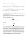

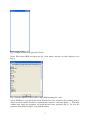
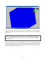
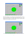

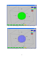
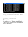
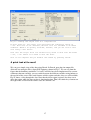
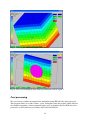
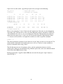
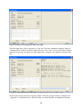
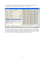
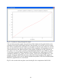
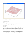

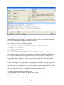
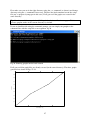
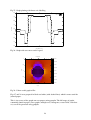

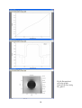
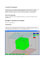
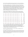
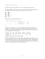
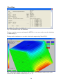
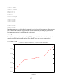
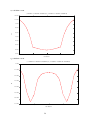
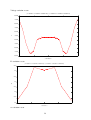
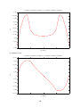
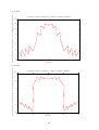
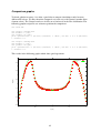
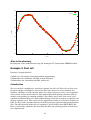
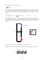

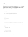
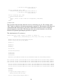
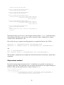
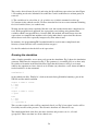
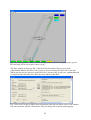
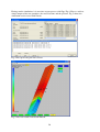
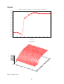
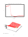
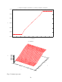
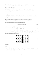


![[U4.84.11] Opérateur POST_DECOLLEMENT](http://vs1.manualzilla.com/store/data/006355898_1-cfc544bde2776e59771a8974d75a4cb3-150x150.png)