Download ZINC 3.2 (Finite element code) User Manual

NPL Report
ZINC 3.2 (Finite element code)
User Manual
John Blackburn
August 2011
NPL Report
ZINC 3.2 (Finite element code)
User Manual
John Blackburn
Materials Group
August 2011
ABSTRACT
This document describes the operation of Zinc, version 3.2. Zinc is a program to solve (nonlinear) multiphysics problems using the finite element method. It can be used to model almost
any physics system.
NPL Report
c Crown copyright 2010
Reproduced with the permission of the Controller of HMSO
and Queen’s Printer for Scotland
National Physical Laboratory,
Hampton Road, Teddington, Middlesex, United Kingdom TW11 0LW
Extracts from this report may be reproduced provided the source is acknowledged and the
extract is not taken out of context
We gratefully acknowledge the financial support of the UK Department for Innovation,
Universities and Skills (National Measurement System Directorate)
Approved on behalf of the Managing Director, NPL by Markys Cain,
Knowledge leader for the Materials Team
ZINC 3.2 user manual
NPL Report
Contents
1 Introduction
1.1 Comparison to other general purpose FE programs . . . . . . . . . . . . . . . . .
1.2 Zinc operation . . . . . . . . . . . . . . . . . . . . . . . . . . . . . . . . . . . . .
1
2
4
2 Installing and running Zinc
2.1 Zinc install directory . . . .
2.2 Uninstalling zinc . . . . . .
2.3 Linux and Mac . . . . . . .
2.4 Zinc Memory requirements
.
.
.
.
7
8
8
8
8
.
.
.
.
.
.
.
.
.
.
.
.
.
.
.
.
.
9
9
11
11
11
12
12
16
17
18
18
19
19
19
21
22
22
22
.
.
.
.
.
.
25
25
26
26
26
27
28
.
.
.
.
.
.
.
.
.
.
.
.
.
.
.
.
.
.
.
.
3 Meshing with Zmesh
3.1 The Zmesh program . . . . . . . . .
3.1.1 File menu . . . . . . . . . . .
3.1.2 View Menu . . . . . . . . . .
3.1.3 On screen controls . . . . . .
3.1.4 Output window . . . . . . . .
3.2 Structure of the geometry input file .
3.3 Neuman Boundaries . . . . . . . . .
3.4 List of part specification commands
3.5 List of global commands . . . . . . .
3.6 List of basic 3D parts . . . . . . . .
3.7 List of open parts . . . . . . . . . . .
3.8 Advanced parts . . . . . . . . . . . .
3.8.1 Extrusion . . . . . . . . . . .
3.8.2 Turning . . . . . . . . . . . .
3.8.3 Transition . . . . . . . . . . .
3.8.4 Neon . . . . . . . . . . . . . .
3.8.5 Summary of advanced shapes
.
.
.
.
.
.
.
.
.
.
.
.
.
.
.
.
.
.
.
.
.
.
.
.
.
.
.
.
.
.
.
.
.
.
.
.
.
.
.
.
.
.
.
.
.
.
.
.
.
.
.
.
.
.
.
.
.
.
.
.
.
.
.
.
.
.
.
.
.
.
.
.
.
.
.
.
.
.
.
.
.
.
.
.
.
.
.
.
.
.
.
.
.
.
.
.
.
.
.
.
.
.
.
.
.
.
.
.
.
.
.
.
.
.
.
.
.
.
.
.
.
.
.
.
.
.
.
.
.
.
.
.
.
.
.
.
.
.
.
.
.
.
.
.
.
.
.
4 PDE specification
4.1 Mode 1: Static problems . . . . . . . . . . . . . .
4.2 Mode 2: Transient problems . . . . . . . . . . . .
4.3 Static and steady state problems . . . . . . . . .
4.4 Example with thermal-electrical coupling . . . .
4.5 Matrix and component form PDE specification .
4.6 Multiferroic equations: a more complex example
i
.
.
.
.
.
.
.
.
.
.
.
.
.
.
.
.
.
.
.
.
.
.
.
.
.
.
.
.
.
.
.
.
.
.
.
.
.
.
.
.
.
.
.
.
.
.
.
.
.
.
.
.
.
.
.
.
.
.
.
.
.
.
.
.
.
.
.
.
.
.
.
.
.
.
.
.
.
.
.
.
.
.
.
.
.
.
.
.
.
.
.
.
.
.
.
.
.
.
.
.
.
.
.
.
.
.
.
.
.
.
.
.
.
.
.
.
.
.
.
.
.
.
.
.
.
.
.
.
.
.
.
.
.
.
.
.
.
.
.
.
.
.
.
.
.
.
.
.
.
.
.
.
.
.
.
.
.
.
.
.
.
.
.
.
.
.
.
.
.
.
.
.
.
.
.
.
.
.
.
.
.
.
.
.
.
.
.
.
.
.
.
.
.
.
.
.
.
.
.
.
.
.
.
.
.
.
.
.
.
.
.
.
.
.
.
.
.
.
.
.
.
.
.
.
.
.
.
.
.
.
.
.
.
.
.
.
.
.
.
.
.
.
.
.
.
.
.
.
.
.
.
.
.
.
.
.
.
.
.
.
.
.
.
.
.
.
.
.
.
.
.
.
.
.
.
.
.
.
.
.
.
.
.
.
.
.
.
.
.
.
.
.
.
.
.
.
.
.
.
.
.
.
.
.
.
.
.
.
.
.
.
.
.
.
.
.
.
.
.
.
.
.
.
.
.
.
.
.
.
.
.
.
.
.
.
.
.
.
.
.
.
.
.
.
.
.
.
.
.
.
.
.
.
.
.
.
.
.
.
.
.
.
.
.
.
.
.
.
.
.
.
.
.
.
.
.
.
.
.
.
.
.
.
.
.
.
.
.
.
.
.
.
.
.
.
.
.
.
.
.
.
.
.
.
.
.
.
.
.
.
.
.
.
.
.
.
.
.
.
.
.
.
.
.
.
.
.
.
.
.
.
.
.
.
.
.
.
.
.
.
.
.
.
.
.
.
.
.
.
.
.
.
.
.
.
.
.
.
.
NPL Report
ZINC 3.2 user manual
5 Zinc (core solver)
5.1 Mesh definition file file.mtf . . . . . . . .
5.2 Material/physics file filename.zin . . . .
5.2.1 Control variables . . . . . . . . . .
5.2.2 Region specification blocks . . . .
5.2.3 Specifying Neumann boundaries at
5.2.4 Initial state specification . . . . . .
5.3 Expressions . . . . . . . . . . . . . . . . .
5.4 The constants file, file.con . . . . . . .
5.5 Advanced, non-linear simulations . . . . .
5.6 Examples of zinc input files . . . . . . . .
5.7 Zinc: output files . . . . . . . . . . . . . .
. . . . .
. . . . .
. . . . .
. . . . .
surfaces
. . . . .
. . . . .
. . . . .
. . . . .
. . . . .
. . . . .
.
.
.
.
.
.
.
.
.
.
.
.
.
.
.
.
.
.
.
.
.
.
.
.
.
.
.
.
.
.
.
.
.
.
.
.
.
.
.
.
.
.
.
.
.
.
.
.
.
.
.
.
.
.
.
.
.
.
.
.
.
.
.
.
.
.
.
.
.
.
.
.
.
.
.
.
.
.
.
.
.
.
.
.
.
.
.
.
.
.
.
.
.
.
.
.
.
.
.
.
.
.
.
.
.
.
.
.
.
.
.
.
.
.
.
.
.
.
.
.
.
.
.
.
.
.
.
.
.
.
.
.
.
.
.
.
.
.
.
.
.
.
.
.
.
.
.
.
.
.
.
.
.
.
.
.
.
.
.
.
.
.
.
.
.
.
.
.
.
.
.
.
.
.
.
.
.
.
.
.
.
.
.
.
.
.
.
31
32
33
34
35
36
37
37
38
39
42
42
6 Zpp: the Zinc post processor
6.1 Zpp input files . . . . . . .
6.2 Scan expressions . . . . . .
6.3 Example calculations . . . .
6.4 Zpp output files . . . . . . .
.
.
.
.
.
.
.
.
.
.
.
.
.
.
.
.
.
.
.
.
.
.
.
.
.
.
.
.
.
.
.
.
.
.
.
.
.
.
.
.
.
.
.
.
.
.
.
.
.
.
.
.
.
.
.
.
.
.
.
.
.
.
.
.
.
.
.
.
.
.
.
.
49
49
51
52
53
.
.
.
.
.
.
.
.
.
.
.
.
.
.
.
.
.
.
.
.
.
.
.
.
.
.
.
.
.
.
.
.
.
.
.
.
.
.
.
.
.
.
.
.
.
.
.
.
A Comsol’s coefficient mode
57
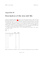
B Description of the zinc.mtf file
59
C Additional global variables in file.zin
63
ii
ZINC 3.2 user manual
NPL Report
Chapter 1
Introduction
Zinc is a finite element code capable of solving a wide range of physics and multiphysics problems. Zinc can solve pretty much any physics based problems which can be expressed as
second order partial differential equations. Examples of physics systems which can be solved
include: electrostatics, magnetics, elastic theory, thermal fluctuation, diffusion etc. Further,
any combination of these physics theories can also be solved as well. Zinc has been successfully used to solve piezoelectric (elastic+electric), multiferroic (elastic+electric+magnetic) and
fuel cells (multiple component diffusion+pressure variation). A near-infinity of other systems
could also be solved including all the most common scenarios in electromangetics, mechanics,
thermodynamics, fluid flow, diffusion and so on. The reason for Zinc’s generality is that it is
fundamentally a mathematical rather than physics program. Zinc solves equations and it is up
to the user to tune those equations to correspond to the needed physics system. This requires a
certain mathematical skill and familiarity with the problem in hand. However, we believe that
no FE code is a substitute for such knowledge: computer modelling is a highly skilled process
and cannot be done without skilled human input. We’ll see fully automated modelling the day
we have lawyer-less courtrooms and doctor-less hospitals! Nonetheless, the level of skill required
to use Zinc is not enormously high. Anyone with a physics, maths or engineering degree should
have no difficulty following the step-by-step instructions in this manual. If users don’t wish to
set up their own problems, they can come to NPL for help. Once a set of input files has been
prepared, it is easy to adapt it to, say, change material properties or geometry without needing
to adjust the detailed physics. Several examples of common physics systems are supplied in the
supplied Tutorial Manual and it should be easy to adapt these for many “bread and butter”
problems. The beauty of Zinc is that it can solve these familiar problems at full speed while
at the same time allowing the simulation of completely new or esoteric equations, which might
never have been written down before, let alone solved!
However, before we get too carried away, we should admit that Zinc, in common with other
general purpose FE packages, cannot necessarily solve any problem input to it. Some problems
will turn out to self-contradictory, a fact which is not always obvious when the equations are
written on paper. Other systems may be unstable giving a very poorly conditioned matrix
and needing special techniques to solve. Zinc comes with several built-in solvers, but users
having particular problems should approach NPL for advice. In some cases, problem-specific
solution techniques may be needed which NPL can possibly provide. We would like to emphasise
that this limitation is not specific to Zinc but is a necessary feature of all general-purpose FE
programs. For example, we have tested Zinc extensively against Comsol. When the equations
Page 1 of 63
NPL Report
ZINC 3.2 user manual
were well-formed, Zinc and Comsol both solved the problem and gave the same answer. When
the equation were not well formed, both solvers failed to converge and terminated with errors.
In general, the only way to see if a set of equations will solve nicely is to try solving them.
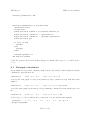
1.1
Comparison to other general purpose FE programs
As mentioned we have tested Zinc against Comsol quite extensively. In Comsol, equations can
be set up in the so-called ”coefficient mode”, the ”strong mode” and the ”weak mode”. Zinc’s
operation mirrors Comsol’s coefficient mode. That is the coefficients in a set of partial differential
equations are set to specify the required mathematical system. A simulation run in Zinc can
therefore be easily transfered to Comsol and vice versa. However, we have not implemented
the ”strong” and ”weak” formulations because most physics problems are naturally formulated
as differential equations. (It has been said that physics is the simply the study of differential
equations). The ”strong” and ”weak” formulations of Comsol are an alternative way of writing
the laws of physics which, however, do not appear naturally in most areas of physics, but
involve reformulating problems using advanced mathematical techniques. Above we’ve said that
it takes first year undergraduate skills to form the Zinc (and Comsol coefficient mode) equations,
but these weak and strong forms are more complex requiring at least PhD in mathematics or
theoretical physics. Given that most physical laws are not written in this way, the ”strong” and
”weak” forms seem both confusing and unnecessary.
However, many users of Comsol never come across these core formulations but are instead
encouraged to ”combine” areas of physics to get the system they need. For example a piezoelectric problem, you would combine the ”elastic” module with the ”electrostatic” module. We
strongly believe that this ”paint by numbers” approach to physics is extremely dangerous and
the user is almost certain to end up simulating something different from what they intended.
This method is therefore not supported in Zinc.
Another general purpose FE package we have some experience of is OpenFOAM. Whereas
Comsol is very much a point-and-click style program, requiring the user to enter data in a
large number of dialog boxes, openFOAM takes the opposite approach, requiring the user to
(re)write large portions of code and recompile openFOAM each time a new physics system is
attempted (specifically, the user rewrites the ”main loop” of the code and calls a large number
of built in functions, the operation of which the user must learn in detail). This provides
enormous flexibility in that the user can alter the fundamental operation of OpenFOAM, but
it also makes it very difficult for people to use the package without specialist help. To use
openFOAM you need, in addition to maths and physics knowledge, considerable understanding
of C++ (the language openFOAM is written in) and you must also study the internal structure
of the openFOAM source code in detail. We can see the advantages that openFOAM has in
terms of flexibility but we think that users should not need to be grandmasters of a particular
programming language to use an FE package. Also the user should not be exposed so much to
the internal workings of the code as they are in OpenFOAM.
In Zinc, we have therefore taken a middle ground. Most users will never need to write
any code to use Zinc. You just set up the coefficients to correspond to the physics/material
properties you want. Running a new physics problem just involves altering the input file: no
programming needed. To support non-linearity, material properties can be entered as expressions
of the variables being solved for. For instance, if you are solving a dielctric problem you can
Page 2 of 63
ZINC 3.2 user manual
NPL Report
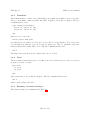
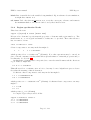
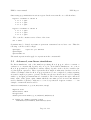
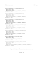
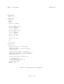
In Fortran:
function cfun(string,x,y,z,ur,dur,nvar,istep)
character(*) string
double precision x,y,z,ur(1),dur(1,3)
integer nvar
if (string.eq.’$permittivity’) Cfun=1+2*ur(1)
end function cfun
! ie, permttivity = 1+2*V
In C:
double cfun(char *label, double *x, double *y, double *z,
double ur[3], double dur[3][1], int *nvar, int *istep, int length)
{
if (equal(label,length,"$permittivity"))
return 1+2*ur[0];
// ie, permittivity = 1+2*V
}
Figure 1.1: Example of functions used in Zinc for non-linear simulation. Fortran and C forms
are showed but any language capable of producing a DLL can be used. Function “equal” is
described in Figure 5.2
set the permittivities to be constants like 1.0 or expressions like 1+2*V (where, for example,
V is the electrostatic potential). In the latter case the problem would be non-linear since the
permittivities depend on the potentials being solved for. Arbitrary expressions may be entered
depending on the solution variables (and their derivatives) and/or space position (x,y,z). For
conveniance the user can also refer to constants (in the .con file, see Section 5.4) which can
be altered between simulations. Thus we can change the shape of the system or its material
properties without going into details within the main ”physics” input file (.zin).
However, sometimes a simple expression like 1+2*V will not be sufficient: it may is necessary
to do a complex calculation with loops and branches to discover the material properties. An
extreme case might involve running a molecular dynamics code to discover the material property.
This code could easily be larger than Zinc itself! Zinc can therefore, optionally, be made to
link to arbitrary code. Instead of setting 1+2*V, the user writes several functions, an example
of which is shown in Figure 1.1.
This function (and a few others like it) is all that is expected from the user even in this
“advanced” method of using Zinc. Note that any programming language can be used provided
it can be compiled into a Dynamic Link Library (DLL). Unlike OpenFOAM, Zinc is deliberately
language agnostic and never needs to be recompiled. The user simply provides a function (in
a DLL) which calculates the needed material property given the point in space x,y,z and the
solved-for variables (ur) and their derivatives (dur). The user is entirely shielded from the inner
working of Zinc, and just needs to fill out a purely mathematical function. Of course instead of
the single line Cfun=1+2*ur(1), as above, the user can enter arbitrarily complex code with loops,
branches, calls to other functions, read/write from files etc. We believe that this approach is
much simpler and more effective than the OpenFOAM technique. Note again that programming
Page 3 of 63
NPL Report
ZINC 3.2 user manual
is optional, and only needed for advanced simulations. Full details of user functions accessed by
Zinc are given in Section 5.3.
1.2
Zinc operation
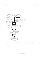
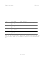
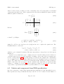
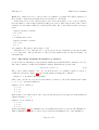
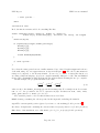
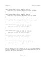
With these ideas in mind, let us look at the operation of Zinc, which is shown diagrammatically
in Figure 1.2. This looks complex but bear with us! The user can choose any stem name
”file” for the simulation. Thus, file.zin might become fuelcellcathode.zin for example.
The file.zin file contains all information about the physics of the problem to be solved.
file.con (optional) contains a list of convenient constants in the simulation which will be
referred in file.zin. Eg, we can store eps0=8.854e-12, the permittivity of free space. The
permittivity of a material with rel. permittivity 2 can then be entered as 2*eps0 rather than
the more cumbersome 1.778e-11. file.dll contains the above-mentioned non-linear functions
(if needed), more details of which are shown in Section 5.5.
Before a geometry can be solved in FE it needs to be broken up into many small shapes
called elements through a process known as meshing. Zmesh provides the functionalilty. The
user writes file.min which specifies the geometry in a simple way. Zmesh then processes this
file and outputs file.mtf which contains the geometry and position of all the elements.
Zinc then runs and writes an output file file.zou containing the solution on each of the
FE nodes. This file can be viewed directly using Zmesh but for more advanced views and post
processing, the code Zpp is provided. Zpp (Zinc post processor) reads the file file.zpp, in
which the user specifies a series of linescans and/or plane scans and generates corresponding
graphs. The user can plot arbitrary expressions based on the simulation variables and their
derivatives. Zpp automatically plots all files on the screen and also creates graph files in the form
of Enhanced Metafiles (EMF) or Encapsulated Postscript (EPS) files. EMF files are convenient
for Microsoft Office products while EPS is most suitable for LATEX: both are vector formats.
In order to generate these graphs, Zpp outputs the datafiles file01.out, file02.out...
etc. These are simply numbered in order created (depending on how many such plots the user has
requested). Zpp then calls Gnuplot (using auto-generated command file file.gnu) to generate
the graphs needed. Since the *.out files are still left behind on disk, its easy to recreate the
graphs when needed. The user can use Gnuplot to change the symbols, titles and formatting of
the graph or to plot several simulation results in one graph. It’s easy, for example, to compare
simulation results with experimental data. Since the raw data files are always on disk there’s
never any mystery about where a graph came from. This approach therefore provides good
traceability and flexiblity. See the Tutorial Manual, Chapter 1 for more details on advanced
graph plotting.
Page 4 of 63
ZINC 3.2 user manual
NPL Report
file.zin
file.min
[file.con]
ZMESH
[file.dll]
file.mtf
file.mls
[file.rst]
ZINC
file.zpp
file.zls
file.zou
ZPP
file01.out
etc
file.gnu
GNUPLOT
file01.eps or
file01.emf etc
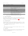
Figure 1.2: The operation of Zinc. Ellipses are files and rectangles are programs. Optional
input files are shown in [brackets]. The DLL file can be generated using any programming
language
Page 5 of 63
NPL Report
ZINC 3.2 user manual
Page 6 of 63
ZINC 3.2 user manual
NPL Report
Chapter 2
Installing and running Zinc
Zinc is installed using an automatic installer which will guide you through the process. The
three programs, Zmesh, Zinc, Zpp, are available to run from the Start Menu in Windows. The
programs can also be invoked from the command line as
zmesh filename
zinc filename
zpp filename
This latter technique is useful for running Zinc under batch control. Zinc can also be run from
external programming systems like Matlab, Python or Excel.
The actual filenames for the Zinc programs are:
zinc.exe Core solver, runs at the command line.
zincwin.exe Windows version of Zinc.
zpp.exe Post processor, runs at the command line.
zppwin.exe Windows version of Zpp.
zmesh.exe Non-interactive mesh generation.
zmeshwin.exe Interactive mesh generation/visualization package.
When Zinc installs, the windows versions of Zmesh, Zinc, and Zpp appear in the Start
Menu. The installer adds Zinc’s directory to your PATH so that you can conveniently run
Zinc from the command prompt. Windows programs like zincwin.exe operate by calling their
command line equivalents, like zinc.exe.
Zinc also comes bundled with Gnuplot. Zpp invokes Gnuplot to generate graphs. Gnuplot is
then available for the user to run independently from Zinc. Gnuplot comes with documentation
and many tutorial examples. Since Zpp emits text output files as well, these can be plotted
using any graph plotter or spreadsheet program. However, we recommend the user of Gnuplot
for best speed and quality.
For advanced, non-linear operation, the user will need to prepare DLL files for Zinc to link
to. A free compiler like gcc or gfortran will do (http://gcc.gnu.org/wiki/GFortran). See
the Tutorial Manual, Chapter 3, for an example of preparing a DLL file to link to Zinc. The
user does not need to recompile Zinc.
Page 7 of 63
NPL Report
2.1
ZINC 3.2 user manual
Zinc install directory
In the install directory you will find the directory examples. This contains several worked
examples which are described in the Tutorial Manual. Also there is a mesh examples directory
which contains various meshing examples (.min files). You should try some of these out in
Zmesh.
Other useful files include nltemplate.f90, nltemplate.c which contain empty user specified functions for non-linear simulations. If you are running an advanced non-linear simulation,
you can create your non-linear functions by copying these templates and filling in the functions
provided.
If you are running Zinc from another system like Python or Matlab, it may be preferable
to run Zinc and Zpp indirectly using the provided batch files zincrun, zpprun. These short
batch files simply ensure that the Zinc, Zpp command prompts stay open should an error occur.
Otherwise you will not be able to read the error before the box closes. Useage:
zincrun file
zpprun file
2.2
Uninstalling zinc
Simply use the “Unistall” icon in the Start Menu. If you install a newer version of Zinc, you
should uninstall the old version first. Note, everything in the Zinc install directory will be
deleted so you should not store simulation runs in the Zinc install directory.
2.3
Linux and Mac
While Zinc has been written for Windows computers, it should run perfectly on Linux and
Mac using the Wine system. Wine comes bundled with most Linux systems and is available for
download on Mac. The Wine website contains comprehensive information on running Windows
programs with Wine. To install Zinc, you should run the installer executable through Wine.
Then run Zmesh, Zinc and Zpp through Wine.
One issue we’ve noticed on Linux: it’s better to install Zinc in a directory without spaces
in its path, i.e., not in the default c:\program files\zinc directory. Similarly the directory
where you store your actual simulations should probably be free of spaces.
2.4
Zinc Memory requirements
Most of Zinc’s memory requirement is due to storing the matrix Q. This is stored in sparse
format in Qval(ip), iQ(ip), jQ(ip), ip=1,...,lenQ where lenQ=nnod*nvar2*27. Here,
nnod, nvar are the total number of nodes and number of variables respectively. Zinc uses
8 byte real numbers (double precision) and 4 byte integers. Therefore each entry in Q uses
8+4+4=16 bytes and the memory requirement is about nnod*nvar2*27*16 bytes.
Page 8 of 63
ZINC 3.2 user manual
NPL Report
Chapter 3
Meshing with Zmesh
Before we can simulate a problem in Zinc, the geometry must first be meshed. This is the process
of decomposing the required geometry into small elements. Zinc requires that the geometry be
meshed into hexahedral elements and this may be accomplished by using the included program
Zmesh. A hexahedron is a six sided solid figures resembling a squashed cube. Cuboids are
special cases of hexahedrons: if the geometry is a laminar system, for example, it may be
sufficient to use cuboid hexahedrons. In general, however, Zmesh will distort the hexahedrons
so as to conform to surfaces in the geometry specified. Zmesh works by reading in the geometry
specification from file file.min and writing out file.mtf which contains the shape and position
of each element. file.mtf is just a text file, whose format is described in Section B, so you can
write your own program to do the meshing if you want. This may be useful in cases where the
geometry consists of irregular shapes. For example, we had a project to model the stress/strain of
ferroelectric domains. We wrote a program to convert the domain map output by a microscopic
imaging device into the corresponding file.mtf. Zmesh would not have been helpful in this
case, since the shapes are irregular and better represented as a “map” rather than a series of
primitive shapes like spheres and boxes.
Zmeshuses the same geometry specification format as MetaMesh, a commercial meshing
program available from Field Precision1 . As such, MetaMesh can be used in place of Zmesh if
required. Metamesh has many more features than Zmesh including a CAD front end and the
ability to read stereo lithography and popular CAD files for geometry specification. Although
more basic, Zmesh will do the job in most systems and at least it’s free! The user may want
to try using Zmesh first, to see whether the Zinc package as a whole is suitable to their needs.
Then, if more sophisticated geometries are needed, the user can opt to purchase MetaMesh
directly from the Field Precision website.
3.1
The Zmesh program
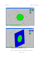
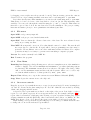
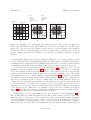
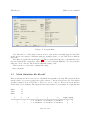
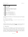
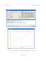
Zmesh is an interactive program as shown in Figure 3.1. The user first prepares an input file,
file.min which contains all the geometry details, Section 3.2. He then uses the File > Open MIN
command to read this file. At this point the file can be examined using File > View MIN. If
all is well, the file can be processed using File > Process. A meshed geometry is then created
and is saved automatically as file.mtf. This geometry appears on screen and can be rotated
1
www.fieldp.com
Page 9 of 63
NPL Report
ZINC 3.2 user manual
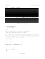
(a) Zmesh view with region 1 turned off to expose region 2
(b) Showing an "xslice" through the structure
Figure 3.1: Zmesh: a program for meshing arbitrary structures.
Page 10 of 63
ZINC 3.2 user manual
NPL Report
by dragging on screen (the arrow keys can also be used). Various viewing options also exist as
described below. A pre-existing mesh file file.mtf can be read using File > open MTF
If you have already run a Zinc simulation, you can view the result using File > open ZOU.
This shows a colour-coded view of the data with a colour bar (on the left) indicating value
variables. You can cycle through the variables using the “¡” and “¿” buttons. This feature is
intended to give a basic look at the raw data solved by the simulation. For post processing,
linescans and surface plots (i.e. more quantitative information) use Zpp.
3.1.1
File menu
Open MIN read geometry input file.
Open MTF read pre-processed mesh definition file.
Open ZOU View a solution file. Shows a basic view of the data. For more advanced views
and post processing, use Zpp.
View MIN Show input file on screen. Note that this file cannot be edited. The user should
use a text editor to edit the file. Notepad will do but a programming text editor may be
preferable. We use Emacs, a free text editor with many advanced features. For complex
geometries it may be necessary to generate file.min using a computer program.
Process Process the currently loaded MIN file.
Exit Terminate the program
3.1.2
View Menu
Bounding box Brings up a dialog allowing user to select a rectangular section of the simulation
volume to display. User selects minimum and maximum i,j,k values (indexing system
for elements). The maximum extents allowed are shown to the right of the dialog. Click
“All” to set the maximum extents and show the whole system. Click “one” to select only
one element which is taken to be that specified by imin, jmin, kmin
Export View Allows you to export the current view as an Enhanced Metafile (EMF).
Copy View Copies the current view to the clipboard.
3.1.3
On screen controls
Drag the on screen objects with the mouse to rotate (or use arrow keys). Zoom in/out using keys
“A” and “Z”. Rotate in the plane using keys “N” and “M”. Shift the view around by holding
“Shift” and dragging with the mouse.
A legend for the region numbers are listed on the right of the screen. Left click to toggle a
region on or off. (when a region is off a cross appears in the box). For example, in Figure 3.1(a),
region 1 has been switched off allowing easier viewing of region 2 (a sphere in this case). When
viewing a simultion result file (ZOU file), these buttons have three states: on, DATA, off. The
DATA state shows colour coded data for the given region with a colour legend on the left.
Right clicking on a region in the legend brings up a colour dialog box which allows the user
to change the colour for the indicated region number.
Page 11 of 63
NPL Report
ZINC 3.2 user manual
The buttons along the bottom are as follows
x,y,z View along the x, y or z axes.
xslice, yslice, zslice View a slice through the system (ie a single plane of elements), for example as shown in Figure 3.1(b). You can change which slice is displayed using the up and
down arrows on the keyboard.
off Switch off slices so that the whole system is displayed.
3.1.4
Output window
Zmesh gives various notifications to the user in the output window. These include, details of
meshing or any errors encountered in the input file.
3.2
Structure of the geometry input file
The mesh input file file.min has the form
global
<global commands>
end
part 1
<part commands>
end
part 2
<part commands>
end
:
endfile
The global commands specifies the logical mesh and various global variables which define the
quality of the meshing. The part commands define various shapes (spheres, cubes, extrusions
etc) that make up the geometry needed. Note that later parts overlap earlier ones so the order
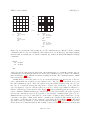
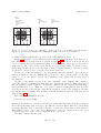
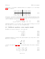
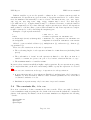
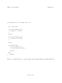
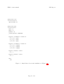
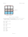
of parts is important. The logical mesh is illustrated in Figure 3.2: it is a simple cuboid mesh
defined by the global commands xmesh, ymesh, zmesh as illustrated in that figure. The logical
mesh defines the number of elements and nodes (intersection of the lines shown) in the simulation
and also the extent of the simulation. In Figure 3.2, for example, the simulation stretches from
−0.5 to 0.5 in all directions. Note that the overall simulation area is always cuboid shaped.
(However, it is possible to model curved outer boundaries by setting the properties of an outer
region to correspond to vacuum). Distance units are not specified at this stage, so the value 0.5
may be metres or angstroms. In Zinc input file file.zin it is possible to scale the geometry
using a scale factor as required, see Section 5.2.1. The global commands xmesh has the form
Page 12 of 63
ZINC 3.2 user manual
NPL Report
0.5
0.1
-0.1
x=-0.5
(a)
0.5
xmesh
-0.5 0.5 0.2
end
ymesh
-0.5 0.5 0.2
end
y=-0.5
x=-0.5
(b)
-0.1
0.1
0.5
xmesh
-0.5 -0.1 0.2
-0.1 0.1 0.033
0.1 0.5 0.2
end
ymesh
-0.5 -0.1 0.2
-0.1 0.1 0.033
0.1 0.5 0.2
end
Figure 3.2: Logical mesh formed using the global commands shown. (In the real file a zmesh
command is also needed. For simplicity, these figures show a 2-D analogy). (a) Single meshing
interval with one xmesh and one ymesh command; (b) variable meshing with multiple meshing
commands
xmesh
x1 x2 dx1
x2 x3 dx2
:
end
where [x1,x2] is a line segment divided into intervals dx1 wide etc. If xmesh contains only one
command line, the meshing is uniform across the whole simulation region. If there are multiple
lines as in Figure 3.2(b), this allows variable meshing as shown. The commands ymesh, zmesh
have exactly the same form.
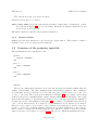
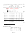
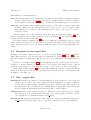
Zmesh then processes the parts one by one as shown in Figure 3.3. In response to the two
part commands shown, a sphere is created inside a cube. The cube is specified first and covers
the whole simulation region. Then, the sphere is specified which is inserted into the cube (ie
the cube is overwritten showing the importance of parts order in the file). Notice that the
cube is designated “region 1” and the sphere as “region 2”. These region numbers will later be
linked to material properties in file.zin. Figure 3.3(a) shows what happens in response to the
part 2 command. Zmesh identifies the elements whose centroids are inside the sphere specified
and sets the elements as region 2. In response to the surface command in the part 2 ’block’,
Zmesh then moves nodes so that they lie on the sphere creating a shape which more closely
conforms to the sphere. Without the surface command, the elements would remain cuboid and
the “sphere” would have the blocky, “staircase” appearance shown in Figure 3.3(a). The final
appearance and region number of each element is shown in Figure 3.3(b). (Note that the picture
shows an inverted elemnent which would actually be fixed by Zmesh. An inverted element has
Page 13 of 63
NPL Report
region 1
ZINC 3.2 user manual
part 2
region 2
type sphere
fab 0.3
end
part 1
region 1
type box
fab 1 1 1
surface region 1
end
region 2
xxxxxxxxxxxxxxxxxxxxxxxxxxxx
xxxxxxxxxxxxxxxxxxxxxxxxxxxx
xxxxxxxxxxxxxxxxxxxxxxxxxxxx
xxxxxxxxxxxxxxxxxxxxxxxxxxxx
xxxxxxxxxxxxxxxxxxxxxxxxxxxx
xxxxxxxxxxxxxxxxxxxxxxxxxxxx
xxxxxxxxxxxxxxxxxxxxxxxxxxxx
xxxxxxxxxxxxxxxxxxxxxxxxxxxx
xxxxxxxxxxxxxxxxxxxxxxxxxxxx
xxxxxxxxxxxxxxxxxxxxxxxxxxxx
xxxxxxxxxxxxxxxxxxxxxxxxxxxx
xxxxxxxxxxxxxxxxxxxxxxxxxxxx
xxxxxxxxxxxxxxxxxxxxxxxxxxxx
xxxxxxxxxxxxxxxxxxxxxxxxxxxx
xxxxxxxxxxxxxxxxxxxxxxxxxxxx
xxxxxxxxxxxxxxxxxxxxxxxxxxxx
xxxxxxxxxxxxxxxxxxxxxxxxxxxx
xxxxxxxxxxxxxxxxxxx
xxxxxxxxxxxxxxxxxxx
xxxxxxxxxxxxxxxxxxx
xxxxxxxxxxxxxxxxxxx
xxxxxxxxxxxxxxxxxxx
xxxxxxxxxxxxxxxxxxx
xxxxxxxxxxxxxxxxxxx
xxxxxxxxxxxxxxxxxxx
(a)
1
1
1
2
xxxxxxxxxxxxxxxxxxxxxxxxxxx
2
xxxxxxxxxxxxxxxxxxxxxxxxxxx
2
1 xxxxxxxxxxxxxxxxxxxxxxxxxxx
xxxxxxxxxxxxxxxxxxxxxxxxxxx
xxxxxxxxxxxxxxxxxxxxxxxxxxx2
xxxxxxxxxxxxxxxxxxxxxxxxxxx
1
1
1
1
1xxxxxxxxxxxxxxxxxxxxxxxxxxx
1
xxxxxxxxxxxxxxxxxxxxxxxxxxx
xxxxxxxxxxxxxxxxxxxxxxxxxxx
xxxxxxxxxxxxxxxxxxxxxxxxxxx
xxxxxxxxxxxxxxxxxxxxxxxxxxx
xxxxxxxxxxxxxxxxxxxxxxxxxxx
xxxxxxxxxxxxxxxxxxxxxxxxxxx
2
2 2
1xxxxxxxxxxxxxxxxxxxxxxxxxxx
xxxxxxxxxxxxxxxxxxxxxxxxxxx
1
xxxxxxxxxxxxxxxxxxxxxxxxxxx
xxxxxxxxxxxxxxxxxxxxxxxxxxx
1
xxxxxxxxxxxxxxxxxxxxxxxxxxx
xxxxxxxxxxxxxxxxxxxxxxxxxxx
xxxxxxxxxxxxxxxxxxxxxxxxxxx
xxxxxxxxxxxxxxxxxxxxxxxxxxx
xxxxxxxxxxxxxxxxxxxxxxxxxxx
xxxxxxxxxxxxxxxxxxxxxxxxxxx
xxxxxxxxxxxxxxxxxxxxxxxxxxx
xxxxxxxxxxxxxxxxxxxxxxxxxxx
xxxxxxxxxxxxxxxxxxxxxxxxxxx
xxxxxxxxxxxxxxxxxxxxxxxxxxx
xxxxxxxxxxxxxxxxxxxxxxxxxxx
xxxxxxxxxxxxxxxxxxxxxxxxxxx
xxxxxxxxxxxxxxxxxxxxxxxxxxx
xxxxxxxxxxxxxxxxxxxxxxxxxxx
xxxxxxxxxxxxxxxxxxxxxxxxxxx
1
1
2
2
1
2
1
2
1*
1
1
1
1
2
1
1
1
1
(b)
1
1
1
xxxxxxxxxxxxxxxxxxxxxxxxxxx
xxxxxxxxxxxxxxxxxxxxxxxxxxx
xxxxxxxxxxxxxxxxxxxxxxxxxxx
xxxxxxxxxxxxxxxxxxxxxxxxxxx
xxxxxxxxxxxxxxxxxxxxxxxxxxx
xxxxxxxxxxxxxxxxxxxxxxxxxxx
xxxxxxxxxxxxxxxxxxxxxxxxxxx
xxxxxxxxxxxxxxxxxxxxxxxxxxx
xxxxxxxxxxxxxxxxxxxxxxxxxxx
xxxxxxxxxxxxxxxxxxxxxxxxxxx
xxxxxxxxxxxxxxxxxxxxxxxxxxx
xxxxxxxxxxxxxxxxxxxxxxxxxxx
xxxxxxxxxxxxxxxxxxxxxxxxxxx
xxxxxxxxxxxxxxxxxxxxxxxxxxx
xxxxxxxxxxxxxxxxxxxxxxxxxxx
xxxxxxxxxxxxxxxxxxxxxxxxxxx
xxxxxxxxxxxxxxxxxxxxxxxxxxx
xxxxxxxxxxxxxxxxxxxxxxxxxxx
xxxxxxxxxxxxxxxxxxxxxxxxxxx
xxxxxxxxxxxxxxxxxxxxxxxxxxx
xxxxxxxxxxxxxxxxxxxxxxxxxxx
2
2
1
1
1
1
1
1
2
2
2
2
2
2
2
2
2
1
1
1
(c)
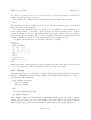
Figure 3.3: Meshing of two parts using the commands shown. The second part (sphere) is
inserted into the initial box part. (a) Identification of element region numbers in original logical
mesh; (b) nodes are moved onto surface between the two regions. Element region numbers
shown. Note that the element marked (*) is not acceptable since it is inverted (see text). In
practice, Zmesh avoids inverted elements or at least gives a warning; (c) Final node region
numbers
a Jacobian which changes sign across the element preventing the code from integrating correctly
over the element (See Theoretical Manual). Zmesh determines whether elements are inverted by
calculating the Jacobian. If it is inverted Zmesh relaxes the lattice to attempt to fix the element
even if that means having a less conforming mesh. A chevron shaped element is inverted)
Nodes are also given “region numbers” as shown in Figure 3.3(c). This is in order to specify
Dirichlet boundary conditions Section 5.2.2 whereby field values are specified on particular
nodes. For example, in an electrostatic problem we could designate region 2 nodes as having
a fixed potential which would make the sphere into a perfectly conducting object. The default
region numbering of nodes – in this example – is shown in Figure 3.3(c): all nodes surrounding
an element are given the same region number as that element. Thus, after processing part 1,
all nodes are designated region 1. After processing part 2, the elements within the sphere are
renumberd region 2 and their surrounding nodes are renumbered region 2 also. In particular the
nodes at the interface between the two regions are set to region 2 (since part 2 was processed
last). In some cases, it is necessary to override this behaviour and give a different region number
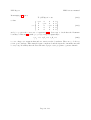
to the interface nodes. This can be accomplished by use of the coat command as shown in
Figure 3.4(a). In this case, while processing part 2, Zmesh gathers all nodes at the interface
between this part and region 1 and numbers these as region 6.
Another way to set node region numbers is to use “open parts” as shown in Figure 3.4(b).
Here we have used two additional parts (3 and 4). These define surfaces at the top and of the
simulation whose nodes are set to region 3 and region 4 respectively. In this example (assuming
an electrostatic problem), it would be possible to excite the system by putting 1 V on region 3
nodes (top, Dirichlet boundary) and zero volts on region 4 nodes (bottom, Dirichlet boundary).
This would create an electric field on the simulation. In elastic problems, this would correspond
Page 14 of 63
ZINC 3.2 user manual
NPL Report
part 2
region 2
type sphere
fab 0.3
surface region 1
coat 1 6
end
part 3
region 3
type boundyup
end
1
1
1
6
xxxxxxxxxxxxxxxxxxxxxxxxxxx
6
6
xxxxxxxxxxxxxxxxxxxxxxxxxxx
1 xxxxxxxxxxxxxxxxxxxxxxxxxxx
xxxxxxxxxxxxxxxxxxxxxxxxxxx6
xxxxxxxxxxxxxxxxxxxxxxxxxxx
1
1
1
1
1
1
xxxxxxxxxxxxxxxxxxxxxxxxxxx
xxxxxxxxxxxxxxxxxxxxxxxxxxx
xxxxxxxxxxxxxxxxxxxxxxxxxxx
xxxxxxxxxxxxxxxxxxxxxxxxxxx
xxxxxxxxxxxxxxxxxxxxxxxxxxx
xxxxxxxxxxxxxxxxxxxxxxxxxxx
xxxxxxxxxxxxxxxxxxxxxxxxxxx
xxxxxxxxxxxxxxxxxxxxxxxxxxx
xxxxxxxxxxxxxxxxxxxxxxxxxxx
xxxxxxxxxxxxxxxxxxxxxxxxxxx
xxxxxxxxxxxxxxxxxxxxxxxxxxx
xxxxxxxxxxxxxxxxxxxxxxxxxxx
xxxxxxxxxxxxxxxxxxxxxxxxxxx
xxxxxxxxxxxxxxxxxxxxxxxxxxx
xxxxxxxxxxxxxxxxxxxxxxxxxxx
xxxxxxxxxxxxxxxxxxxxxxxxxxx
xxxxxxxxxxxxxxxxxxxxxxxxxxx
xxxxxxxxxxxxxxxxxxxxxxxxxxx
xxxxxxxxxxxxxxxxxxxxxxxxxxx
xxxxxxxxxxxxxxxxxxxxxxxxxxx
xxxxxxxxxxxxxxxxxxxxxxxxxxx
xxxxxxxxxxxxxxxxxxxxxxxxxxx
6
2
6
2
6
1
6
1
2
6
6
1
6
6
1
3
1
1
1
1
1
1
1
1
1
1
1
4
(a)
3
part 4
region 4
type boundydn
end
3
2
3
3
3
xxxxxxxxxxxxxxxxxxxxxxxxxxx
xxxxxxxxxxxxxxxxxxxxxxxxxxx
xxxxxxxxxxxxxxxxxxxxxxxxxxx
xxxxxxxxxxxxxxxxxxxxxxxxxxx
xxxxxxxxxxxxxxxxxxxxxxxxxxx
xxxxxxxxxxxxxxxxxxxxxxxxxxx
xxxxxxxxxxxxxxxxxxxxxxxxxxx
xxxxxxxxxxxxxxxxxxxxxxxxxxx
xxxxxxxxxxxxxxxxxxxxxxxxxxx
xxxxxxxxxxxxxxxxxxxxxxxxxxx
xxxxxxxxxxxxxxxxxxxxxxxxxxx
xxxxxxxxxxxxxxxxxxxxxxxxxxx
xxxxxxxxxxxxxxxxxxxxxxxxxxx
xxxxxxxxxxxxxxxxxxxxxxxxxxx
xxxxxxxxxxxxxxxxxxxxxxxxxxx
xxxxxxxxxxxxxxxxxxxxxxxxxxx
xxxxxxxxxxxxxxxxxxxxxxxxxxx
xxxxxxxxxxxxxxxxxxxxxxxxxxx
xxxxxxxxxxxxxxxxxxxxxxxxxxx
xxxxxxxxxxxxxxxxxxxxxxxxxxx
xxxxxxxxxxxxxxxxxxxxxxxxxxx
xxxxxxxxxxxxxxxxxxxxxxxxxxx
xxxxxxxxxxxxxxxxxxxxxxxxxxx
xxxxxxxxxxxxxxxxxxxxxxxxxxx
xxxxxxxxxxxxxxxxxxxxxxxxxxx
xxxxxxxxxxxxxxxxxxxxxxxxxxx
xxxxxxxxxxxxxxxxxxxxxxxxxxx
2
2
1
1
4
4
4
4
2
2
2
2
2
2
2
2
1
2
1
2
2
2
4
1
(b)
Figure 3.4: (a) Use of the coat command to change the node region numbers at an interface;
(b) use of open parts (boundyup and boundydn) to change the node region numbers
to clamped displacements at the top and bottom of the simulation, and so on.
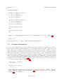
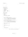
Figure 3.5 shows the corresponding file.zin for Figure 3.4 set up as an electrostatic problem. This file will be described in more detail in Section 5.2 but for now note how region 1 and
region 2 elements are given permittivity values of ǫ0 (permittivity of free space, 8.854 × 10−12
F/m) and 2ǫ0 . Also, region 3 and region 4 nodes are set to voltage values 1 V and 0 V respectively. Region 1 and 2 nodes are not set at all, so these nodes (the interior nodes in the problem)
are allowed to vary in order to solve the electrostatic equations.
By the end of the part fitting process, all elements and nodes should be given an region
number. If this is not the case, Zmesh will report an error. It is common practice for the first
part to be a box part which covers the whole simulation area. Other parts are then inserted
into this part.
We have so far described most of the part commands: type, region, fab, surface,
coat. The other two commands are shift and rotate, allowing the part to be shifted and rotated
into the required position. Parts are conceptually constructed at the origin (0, 0, 0) with major
axes generally along x, y, z. Thus, the “box” part is constructed with principle axes along the
x,y,z directions. It is centred at the origin and its extents are given by the 3 numbers following
the fab (fabricate) command. The meaning of the fab parameters depends on the part and is
given in Table 3.1.
The rotation command has the form
rotate rx ry rz [string]
If string is absent then a rotation is performed about the (global) x-axis, then the y-axis then
the z-axis by the angle given, in degrees. If a different order is required, this can be given using
the string. Eg using “yzx” would cause rotation to occur about y, then z then x. Since these are
Euler angles, rotation order is important. Furthermore, rotation is performed before the object
is shifted irrespective of the order of commands in the part block.
The shift command has the form
Page 15 of 63
NPL Report
ZINC 3.2 user manual
<global commands>
:
region 1 elements 3 values C
V x V x = 8.854e-12
V y V y = 8.854e-12
V z V z = 8.854e-12
region 2 elements 3 values C
V x V x = 1.7708e-11
V y V y = 1.7708e-11
V z V z = 1.7708e-11
region 3 nodes 1 value
V=1
region 4 nodes 1 value
V=0
Figure 3.5: Sample Zinc input file, file.zin corresponding to the setup of Figure 3.4(b)
shift x y z
and causes the part to be shifted along the displacement specified.
3.3
Neuman Boundaries
So far we have discussed the creation of elements and nodes and their region numbers, which are
later associated with volumetric material properties and Neuman boundary conditions respectively. The other boundary condition supported by Zinc is the Neuman boundary condition.
Whereas Dirichlet boundaries fix the variables being solved for, eg, voltage, temperature, elastic
displacement, Neuman boundaries fix derivatives of these: surface charge, thermal flux, traction
respectively. These quantities may be classified as fluxes or applied forces of some kind. Thus
fluxes are applied at boundaries which may be internal to the simulation or external. Zmesh
does not specify such surfaces explicitly, rather surfaces exist between volumetric regions. For
example, the curved surface in Figure 3.4(b) between region 1 and region 2 would be identified
1 − 2 giving an extra command in Figure 3.5
surface 1-2 1 value q
V V = 1.0
surface 1-2 1 value g
V = 2
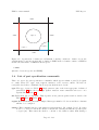
The simulation is conceptually surrounded by regions called “XMAX”, “XMIN”, “YMAX”,
“YMIN”, “ZMAX”, “ZMIN”, as shown in Figure 3.6. Thus the red outer edge on the left hand
of Figure 3.6 can be designated
Page 16 of 63
ZINC 3.2 user manual
NPL Report
YMAX
XMIN
XMAX
region 2
region 3
region 1
YMIN
Figure 3.6: Specification of surfaces for Neumann boundary conditions. Surface 1-2 is the
circular surface between regions 1 and 2. Surface 1-XMIN is the red surface, surface 3-YMIN is
shown blue and surface 3-XMAX is shown green
1-XMIN
(interface between region 1 and XMIN).
3.4
List of part specification commands
There are seven (7) part specification commands which appear within a part block (part
n...end). These are: type, fab, region, surface, coat, rotate, shift. We have already introduced these commands but now specify them in more detail
type The type of part, see Table 3.1. Single parts are just of the form type part. Advanced
parts Table 3.3 have the form type <part> <Vector list> end with each vector on a
separate line, Section 3.8.
fab Fabrication info for the part. This depends on the part in question and is described in
Table 3.1, Table 3.2, Table 3.3.
region Elements in this part will be assigned this region number. Nodes around those elements
will also be so assigned.
surface This command has the form surface {region|part} [n] {edge} [tol]. It causes
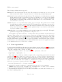
nodes to be moved towards the surface between the current part and the specified part
or region (n). This causes the mesh to conform to the surfaces rather than having a
Page 17 of 63
NPL Report
ZINC 3.2 user manual
“staircase” appearance. The edge command causes edge fitting to take place also. If
present, tol determines the speed of relaxation onto the surface. It is a number in the
range 0-1. If omitted, the default value is 0.9 is assumed
coat Has the form coat reg regnew. Finds all nodes at the interface between the current part
and region reg. These nodes are then given region number regnew.
rotate Has the form rotate x y z {string}. By default, rotate part about the x, y and z
axes in that order (angles in degrees). If string is present, the order of rotation may be
altered. Eg xzy means rotate about x, then about z, then about y. The order of rotation
is important: x,y and z are Euler angles. Rotation is performed before shifting.
shift shift x y z shift the part along the vector specified after rotation is complete.
protect Protects node region numbers in current part from being overwritten. This is useful in
filled parts whose nodes might be overwritten by open parts. Since open parts are always
processed after filled parts, it is not possible to simply rearrange the parts order. This
only affects node, not elements.
3.5
List of global commands
These commands must appear in the global section of the input file.
xmesh, ymesh, zmesh Specified line segments spanning the simulation area in the x direction.
This defines the logical mesh. Each line segment is divided into intervals allowing variable
meshing. Has the form xmesh <line segments> end with each line segment on a separate
line of the form x1 x2 dx. Commands ymesh, zmesh have the same form.
presmooth N Smooths the logical mesh using N smoothing steps. This is only important
when variable resolution is used in the logical mesh. Default: no smoothing.
axissmooth dir N Smooths along one direction “dir” only. Dir is either x, y, or z. N is the
number of steps. Default: no axis smoothing.
smooth N Smooths the final mesh after part fitting has been accomplished. N steps of relaxation, default 10.
format Format {ascii|binary} causes the mesh output file to be text (file.mtf) or binary
(file.mdf) respectively.
3.6
List of basic 3D parts
These parts may be rotated/shifted into position using rotate and shift commands. They are
listed in Table 3.1.
Page 18 of 63
ZINC 3.2 user manual
Shape
box
sphere
cylinder
cone
Fab parameters
Lx Ly Lz
R
RH
R H Hz
ellipcyl
Rx Ry H
ellipsoid
torus
Rx Ry Rz
Rr
helix
R r H Hw
trapezoid
LxU LxD Ly Lz
NPL Report
Description
Centred at origin and extends [-Lx,Lx] along x etc
Centred at origin with radius R
Centred at origin with radius R and extends [-H/2,H/2] along z
Truncated cone along z with base at z = 0 with radius R.
Apex at z = H and truncated at z = Hz
Cylinder along z with elliptical cross section extending
x=[-Rx,Rx], y=[-Ry,Ry]
Ellipsoid given by (x/Rx )2 + (y/Ry )2 + (z/Rz )2 = 1
R is major radius and r is minor radius.
Plane of the “hole” is normal to z
Circular cross section helix (radius r) which wraps around
a z-directed cylinder height H, radius R centred at the origin.
Hw is the height along z attained during 1 revolution.
Prism along z with trapezoidal cross section.
Full width in x is LxU (top) and LxD (bottom).
Full width in y and z given by Ly, Lz
Table 3.1: List of 3-D parts and the meaning of the fab command
3.7
List of open parts
These parts have no volume so elements are not effected. The only result is to change the region
numbers of nodes. These parts are 0, 1 or 2-D and may be rotated and shifted into position
using rotate and shift commands. Note that boundxup etc do not need fab commands and
are unaffected by rotate and shift. The parts are listed in Table 3.2.
3.8
Advanced parts
Zmesh supports 4 types of advanced parts which allow more general shapes to be created:
extrusion, turning, transition and neon. Whereas the simple parts above have a single
line type command (E.g. type sphere), these parts have a multi-line type command of the form,
type {extrusion|turning|transition|neon}
<data lines>
:
end
Apart from this, the part specification is the same and region, surface, coat, shift,
rotate commands may be used as usual.
3.8.1
Extrusion
An extrusion is a prism shape along the z axis. The cross section is built up using an arbitrary
number of line or arc segments which must form a closed 2-d shape in the x-y plane.
The type command has the form
Page 19 of 63
NPL Report
ZINC 3.2 user manual
Part
point
boundxup
boundxdn
boundyup
boundydn
boundzup
boundzdn
line
arc
fab params
xyz
(none)
(none)
(none)
(none)
(none)
(none)
L
R θmin θmax
circle
rectangle
disk
plate
bubble
R
Lx Ly
R
Lx Ly
R
Description
Creates a point at (x,y,z)
plate comprising the upper x plane of the simulation
plate comprising the lower x plane of the simulation
plate comprising the upper y plane of the simulation
plate comprising the lower y plane of the simulation
plate comprising the upper z plane of the simulation
plate comprising the lower z plane of the simulation
line from (0,0,-L/2) to (0,0,L/2)
Arc in z=0 plane centred at origin from angle
θmin to θmin , radius R. θ = 0 is the x-axis. Angles in degrees.
open circle centred at origin radius R
Open rectangle in z=0 from [-Lx,Lx] in x and [-Ly,Ly] in y
As circle but filled
As rectangle but filled
Spherical surface centred at origin radius R
Table 3.2: List of open parts
type extrusion {sidefit}
Vector 1 {S|SE}
Vector 2 {S|SE}
:
end
Each vector describes a line or arc in the x-y plane and is of the form
{L|A} xstart ystart xend yend {xcentre ycentre}
Here, “L” means line and “A” means arc. The xcentre ycentre specification is only required
for arcs. The line extends from (xstart,ystart) to (xend,yend) with arc centre (in the case
of arcs) at (xcentre,ycentre). Vectors should link to one another in sequence and form a
closed loop in the x-y plane. Eg to make a square use
type extrusion
L 0 0
1 0
L 1 0
1 1
L 1 1
0 1
L 0 1
0 0
end
To make a circle, we could adapt this to read
type extrusion
A 0 0 1 0 0.5
A 1 0 1 1 0.5
A 1 1 0 1 0.5
A 0 1 0 0 0.5
end
0.5
0.5
0.5
0.5
Page 20 of 63
ZINC 3.2 user manual
NPL Report
Note that arc segments may not be more the 90 degrees. Longer arcs should be divided into
smaller ones just as we have done here.
The extrusion fab command takes a single parameter: the length of the extrusion.
fab L
The extrusion is along the z axis from -L/2 to L/2. The whole extrusion can be rotated and
shifted into place in the usual way.
The S and SE commands at the end of each vector determine how surface fitting is done
on the extruded surface of the shape. If S is present, the segment is surface fitted. If SE is
present edge fitting is done also. Such surface fitting is performed only if a surface command
appears in the part specification. The top and bottom part of the surface is always fitted if such
a surface command is present. To turn off this fitting, use the sidefit specifier.
A complete part specification for extrusion looks like, for example,
part 1
region 1
type extrusion
L -1 0
1 0
A
1 0
0 1
0 0
A
0 1 -1 0
0 0
end
fab 1
rotate 90 0 0
shift 1.0 0.0 0.0
end
This creates prism of semi-circular cross section, length 1 along the z axis, then rotates it around
x so it now points along y. The part is shifted so that its centre is at (1,0,0).
3.8.2
Turning
A turning part is made by constructing a 2-D shape in (r,z) plane then rotating about the z-axis.
The type command has exactly the same form as for the extrusion (including the use of lines or
arcs and the S/SE commands):
type turning {sidefit}
Vector 1 {S|SE}
Vector 2 {S|SE}
:
end
The fab command has the form
fab angmin angmax
where angmin, angmax are the minimum and maximum turning angles (about the z axis) in
degrees. Use 0 and 360 to produce a full turning. If the angle difference is less than 360 the
turning will have “start” and “end” faces which are fitted according to the surface command
(unless sidefit is specified). The turning may be shifted and rotated in the usual way.
Page 21 of 63
NPL Report
3.8.3
ZINC 3.2 user manual
Transition
The transition shape consists of two planar shapes at z=zmin and z=zmax connected together.
As we go from zmin to zmax, the shape smoothly “morphs” between the two shapes. The type
command has the form
type transition {sidefit}
Vector 1a Vector 1b {S}
Vector 2a Vector 2b {S}
:
end
Each vector is of the form
xstart ystart xend yend
Note that arcs are not allowed so there is no need for the L or A specification. Vector 1a (on the
bottom surface) morphs into vector 1b (on the top surface) etc. The “S” parameter, if present,
indicates that surface fitting will be done. The fab command has the form
fab L
The shape then extends along the z axis from z=-L/2 to z=L/2.
3.8.4
Neon
The neon shape is an arbitrary tube of circular cross section. The trajectory of the cross section
is given by a series of points:
part neon
x1 y1 z1
x2 y2 z2
:
end
where (x1,y1,z1) etc are points in 3-D space. The fab command has the form
fab r
where r is the radius of the tube.
3.8.5
Summary of advanced shapes
The advanced shapes are summarised in Table 3.3.
Page 22 of 63
ZINC 3.2 user manual
type
extrusion
turning
transition
neon
type command
type extrusion {sidefit}
[Vector list]
end
type turning {sidefit}
[Vector list]
end
type transition {sidefit}
[Vector pair list]
end
type neon
[points list]
end
NPL Report
fab
L
Description
extrusion from z=-L/2 to z=L/2
θ1 θ2
turning about z from θ1 to θ2 (◦ )
L
transition along z from z=-L/2 to L/2
r
Circular tube radius r
Table 3.3: Table of advanced shapes. A Vector has the form xstart ystart xend yend
{xcentre ycentre} {S|SE}. A Vector pair has the form xstarta ystarta xstartb ystartb
{S}
Page 23 of 63
NPL Report
ZINC 3.2 user manual
Page 24 of 63
ZINC 3.2 user manual
NPL Report
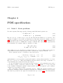
Chapter 4
PDE specification
4.1
Mode 1: Static problems
For static systems, Zinc supports the following partial differential equation sets
− ∇ · C∇u + au = f
(4.1)
n · C∇u + qu = g, (Neumann)
(4.2)
Here u = (u1 , u2 , ...) where u1 (x, y, z) etc are the independent variables to be solved for. For
example u1 might be electrostatic potential and u2 temperature (as in the example of Section
4.4). One must set the various components of C, a, f, q, g so that, when (4.1) is multiplied out,
we obtain the needed set of PDEs and boundary conditions. Here, the meaning of grad and div
is non-standard. For example, with two variables, we define
∇u = (∇u1 , ∇u2 )
(4.3)
∇ · (a|b) = (∇ · a, ∇ · b)
(4.4)
where (a|b) is a 6-vector (in 3D space) partitioned into two, 3-vectors. Thus, grad is applied to
each element in u and div takes groups of three variables and compacts them into one.
These equations can also be written in component form as
− (Cijkl uk,l ),j + aik uk = fi ,
i = 1, . . . , N
(4.5)
nj Cijkl uk,l + qik uk = gi , Neumann i = 1, . . . , N
(4.6)
with summation over repeat indices and N is the number of independent variables to be solved.
Here uk,l = ∂uk /∂xl etc. This general PDE specification allows a wide range of systems to be
solved including those mentioned in the introduction.
To give an example, in an electrostatics problem, setting C to the permittivity tensor and f
to the charge density ρ defines the equation ∇ · D = ρ and (4.2) (with q = g = 0) corresponds
to the “natural”, Neumann boundary condition n · D = 0 which is a typical “open boundary”
condition for electrostatic problems.
The components of C, a, f, q, g all vary in space. When the system is meshed, it is
divided into a structured mesh of hexahedral elements each of which is assigned a region number.
The mesh is specified in the input file filename.mtf (see Section 5.1). The materials file
Page 25 of 63
NPL Report
ZINC 3.2 user manual
filename.zin specifies C, a, f, q, g values for each region, thus specifying material properties
(such as permittivity in the above example) for each element.
The values of C, a, f, q, g components may be set to constant values or set to vary depending
on the local values of the u vector. For example, they might be temperature dependent, in a
thermal problem. In this case, the problem becomes non-linear Section 5.5.
Comsol implements a similar set of equations: these are described in Appendix A. A problem
set in Zinc may easily be converted to Comsol and vice versa.
4.2
Mode 2: Transient problems
Zinc can solve transient problems of the form
∂u
= ∇ · C∇u − au + f
∂t
n · C∇u + qu = g, (Neumann)
(4.7)
(4.8)
or, in component format
∂us
= (Csjkl uk,l ),j − ask uk + fs , s = 1, 2, .., N
∂t
nj Cijkl uk,l + gik uk = gi , Neumann i = 1, . . . , N
(4.9)
(4.10)
Note that the boundary conditions are the same as in the static case. Again, one can set up
either linear or non-linear problems.
4.3
Static and steady state problems
The static mode of Zinc can be made to solve steady state problems as well. Consider the
problem where the u variables depend on time as
u(r, t) = Re[uω (r) exp(jωt)]
(4.11)
In that case we replace ∂/∂t with jωt in the PDEs and the problem again becomes spatial
but we are solving for the phasors uω (r). These phasors are complex numbers whose modulus
indicates time-oscillation amplitude and whose phase gives a phase shift according to (4.11).
However, Zinc does not support complex variables so it will be necessary to write u = ur + iui
and expand each complex equation in terms of two real equations.
Some harmonic problems give real solutions, for example if the material properties are real
(lossless). In that case uω (r) gives amplitudes of oscillation with each point oscillating in phase.
4.4
Example with thermal-electrical coupling
A simple example of how to set the matrices is an electrical conduction/thermal system. In this
case we have
∂V
∂
σ11
−
−
∂x
∂x
∂
∂T
−
k11
−
∂x
∂x
∂
∂V
∂
∂V
σ22
−
σ33
=0
∂y
∂y
∂z
∂z
∂
∂T
∂
∂T
k22
−
k33
=Q
∂y
∂y
∂z
∂z
Page 26 of 63
(4.12)
(4.13)
ZINC 3.2 user manual
NPL Report
where V is the electric potential, σij is the conductivity tensor, T is temperature, k is thermal
conductivity, Q is heat source. These equations follow directly from Maxwell’s equation and the
diffusion equation. In this case,
!
V
u=
(4.14)
T

We have




C=



σ11 0
0
0 σ22 0
0
0 σ33
0
0
0
0
0
0
0
0
0
∇u =
so that ∇ · (−C∇u) is
∇V
∇T
!
0
0
0
k
0
0





=



0
0
0
0
k
0
V,1
V,2
V,3
T,1
T,2
T,3
0
0
0
0
0
k









(4.15)









−(σ11 V,1 ),1 − (σ22 V,2 ),2 − (σ33 V,3 ),3
−(kT,1 ),1 − (kT,2 ),2 − (kT,3 ),3
(4.16)
!
(4.17)
(using V,1 = ∂V /∂x1 etc). And we set f = (0, Q) and a = 0 to complete the equation set. The
Neumann BCs are of the form
n1 σ11 V,1 + n2 σ22 V,2 + n3 σ33 V,3 = 0
(4.18)
n1 kT,1 + n2 kT,2 + n3 kT,3 = 0
(4.19)
which are open or natural boundaries. The latter states that no energy flows out of the system
(insulator).
It may be noted that there is no coupling between V and T in this problem. In fact we
could have just solved for V and T separately. Coupling could be introduced by putting some
non-zero off diagonals in (4.15) or by introducing non-linearity. For example, the conductivities
σ11 etc might depend on temperature while the heat source Q might depend on electric field
(eg Q ∼ E 2 ). Zinc can solve non-linear problems such as this. In linear problems we must set
all the components of C, a, f, q, g to literal constants in the input files (or expressions that
evaluate to constants, see Section 5.3). In non-linear problems we can set some or all of the
components to expressions involving the dependent variables. See Section 5.5.
4.5
Matrix and component form PDE specification
It is often convenient to consider C as a matrix when specifying the problem. Internally, however,
Zinc regards it as being a 4 dimensional array of size N × d × N × d where N is the number of
Page 27 of 63
NPL Report
ZINC 3.2 user manual
variables and d = 3, the number of dimensions. In the above example N = 2, d = 3, the matrix
(4.15) can be written as









C1111
C1211
C1311
C2111
C2211
C2311
C1112
C1212
C1312
C2112
C2212
C2312
C1113
C1213
C1313
C2113
C2213
C2313
C1121
C1221
C1321
C2121
C2221
C2321
C1122
C1222
C1322
C2122
C2222
C2322
C1123
C1223
C1323
C2123
C2223
C2323









(4.20)
and it is these components Cijkl which must be entered in Zinc’s input file. In this way, C may
be written as a series of 3 × 3 “blocks” with the 1st and 3rd component indicating the index of
each block. Written in component form, (4.1), (4.2) become,
− (Cijkl uk,l ),j + aik uk = fi ,
i = 1, . . . , N
(4.21)
nj Cijkl uk,l + qik uk = gi , Neumann i = 1, . . . , N
(4.22)
with implied summation over repeat indices. Also, a, q are matrices and f , g are vectors and
their components aik , qik and fi , gi are entered straightforwardly.
4.6
Multiferroic equations: a more complex example
In multiferroics, frequency domain (∂/∂t → jω) we may write
σij,j + pi = −ρω 2 ui
(4.23)
∇·B=0
(4.25)
∇×H=0
(4.27)
∇·D=0
(4.24)
∇×E = 0
(4.26)
(with Einstein summation convention). The equations assume no space charge and no current.
In this case we can introduce
E = −∇V
H = −∇Vm
1
ǫij = (ui,j + uj,i )
2
(4.28)
(4.29)
(4.30)
so that the curl equations (4.26), (4.27) are automatically satisfied. We use linear constitutive
laws as
m
σij = cEH
ijkl ǫkl − ekij Ek − ekij Hk
Di = eijk ǫjk +
κǫH
ij Ej
(4.31)
+ αij Hj
(4.32)
ǫE
Bi = em
ijk ǫjk + αji Ej + µij Hj
(4.33)
Page 28 of 63
ZINC 3.2 user manual
NPL Report
so that the magnetic and electric equations
in matrix form as

 
σ
cEH

 
 D = e
em
B
look just the same. The equations can be written
−eT
κǫH
αT


ǫ
−(em )T


α
 E 
H
µǫE
(4.34)
Substituting (4.31)-(4.33) in (4.23)-(4.25) and using (4.28)-(4.30), we obtain 5 PDEs
1 EH
+ pi = −ρω 2 ui
c (uk,l + ul,k ) + ekij V,k + em
kij Vm,k
2 ijkl
,j
1
ǫ,H
= 0
eijk (uj,k + uk,j ) − κij V,j − αij Vm,j
2
,i
1 m
= 0
eijk (uj,k + uk,j ) − αji V,j − µǫ,E
V
m,j
ij
2
,i
i = 1, 2, 3
(4.35)
To input these in Zinc we use the following C matrix (omitting some superscripts for clarity)






























c11
c61
c51
c61
c21
c41
c51
c41
c31
e11
e21
e31
em
11
em
21
em
31
c16
c66
c56
c66
c26
c46
c56
c46
c36
e16
e26
e36
em
16
em
26
em
36
c15
c65
c55
c65
c25
c45
c55
c45
c35
e15
e25
e35
em
15
em
25
em
35
c16
c66
c56
c66
c26
c46
c56
c46
c36
e16
e26
e36
em
16
em
26
em
36
c12
c62
c52
c62
c22
c42
c52
c42
c32
e12
e22
e32
em
12
em
22
em
32
c14
c64
c54
c64
c24
c44
c54
c44
c34
e14
e24
e34
em
14
em
24
em
34
c15
c65
c55
c65
c25
c45
c55
c45
c35
e15
e25
e35
em
15
em
25
em
35
c14
c64
c54
c64
c24
c44
c54
c44
c34
e14
e24
e34
em
14
em
24
em
34
c13
c63
c53
c63
c23
c43
c53
c43
c33
e13
e23
e33
em
13
em
23
em
33
e11
e16
e15
e16
e12
e14
e15
e14
e13
−κ11
−κ21
−κ31
−α11
−α12
−α13
e21
e26
e25
e26
e22
e24
e25
e24
e23
−κ12
−κ22
−κ32
−α21
−α22
−α23
e31
e36
e35
e36
e32
e34
e35
e34
e33
−κ13
−κ23
−κ33
−α31
−α32
−α33
em
11
em
16
em
15
em
16
em
12
em
14
em
15
em
14
em
13
−α11
−α21
−α31
−µ11
−µ21
−µ31
em
21
em
26
em
25
em
26
em
22
em
24
em
25
em
24
em
23
−α12
−α22
−α32
−µ12
−µ22
−µ32
em
31

em
36 

em
35 


em
36 
m
e32 


em
34 

m
e35 


em
34 
m
e33 


−α13 

−α23 

−α33 

−µ13 


−µ23 
−µ33
(4.36)

where we use the matrix representation
tensor
matrix
11
1
22
2
33
3
23,32
4
13,31
5
12,21
6
so that c1213 = c65 etc. Of course c is not to be confused with C, the Zinc PDE matrix.
The C matrix above is such that
 h1
m
2 c1jkl (uk,l + ul,k ) + ek1j V,k + ek1j Vm,k
i
 h
i,j
 1
V
 2 c2jkl (uk,l + ul,k ) + ek2j V,k + em
k2j m,k ,j
 h
i
 1
m V
c
(u
+
u
)
+
e
V
+
e
∇ · (C∇u) = 
l,k
k3j ,k
k3j m,k ,j
 2h 3jkl k,l
i

1

e
(u
+
u
)
−
κ
V
−
α
V
ij
,j
ij
m,j
ijk j,k
k,j

 h2
i,i
1 m
2 eijk (uj,k
+ uk,j ) − αji V,j − µij Vm,j
Page 29 of 63
,i












(4.37)
NPL Report
ZINC 3.2 user manual
Rearranging (4.1) gives,
∇ · (C∇u) + f = au
so that




a=


−ρω 2
0
0
0
−ρω 2
0
0
0
−ρω 2
0
0
0
0
0
0
(4.38)
0
0
0
0
0
0
0
0
0
0







(4.39)
and fi = pi gives the correct set of equations (4.35). It is easy to check that the Neumann
boundary condition (4.2) (with q = g = 0) corresponds physically to
nj σij = 0, ni Di = 0, ni Bi = 0
(4.40)
i.e., zero charge, zero magnetic flux and zero traction at the boundaries. These are good choices
for an open boundary. This example if quite complicated and the input file, filename.zin will
be very long. It is likely that the user will write a preprocessor program to generate this file.
Page 30 of 63
ZINC 3.2 user manual
NPL Report
Chapter 5
Zinc (core solver)
Zinc has two basic input files, a geometry file (filename.mtf) specifying the system mesh;
and a materials file (filename.zin) specifying material properties, physics, initial state, boundary conditions and convergence information. There are three optional files: a file containing
constants (filename.con); a restart file filename.rst for specifying the initial state if not
supplied in filename.zin, see key rdu; and filename.dll which contains non-linear functions
if needed. Regarding the restart file, to continue from a previous run, copy filename.zou to
filename.rst. In this case, you will need to set key rdu=1 in file filename.zin.
Zinc outputs two major files (filename.zou, filename.zls). The output file filename.zou
contains the value of each of the variables solved for at each node (in static/steady state problems,
this file contains just the final snapshot, in transient problems it contains several intermediate
snapshots showing the time evolution, see nstride below). filename.zls contains the full set
of input data and information on the convergence etc of the run.
The information in filename.zou is not directly useable for graph plotting. Accordingly a
post processor has been prepared, Zpp, which reads filename.zou as prepared by Zinc and
outputs a series of scans through the data, see Chapter 6.
Zinc also, optionally, exports files in ParaView format (see key export below). Paraview is
a powerful and free post processor that allows 3-D visualization of the simulation results. For
static runs, just one paraview file, filename.vtk, is output corresponding to the final state.
In transient runs, snapshots are output every nstride timesteps. These are written to files
filenamexx.vtk, where xx is 1,2,3...
The normal procedure for using Zinc is
1. Prepare filename.mtf (generated by Zmesh or another program), filename.zin, filename.con
for simulation
2. Run Zinc.
3. Prepare filename.zpp for post processing scans
4. Run Zpp to generate scans through the data. Zpp can automatically create graphs or
these files can be plotted with a graph plotter or spreadsheet of the user’s preference.
5. Alternatively, results can be output and viewed with Paraview
Page 31 of 63
NPL Report
ZINC 3.2 user manual
Figure 5.1: Program Zinc
If a different set of line/plane scans is needed, just update filename.zpp and run Zpp
again. It is not necessary to run Zinc again if you simply want to see the data along a different
direction!
The Zinc program is shown in Figure 5.1. The program allows the user to marshal and view
the various input and output files. Click “open” to select an input (ZIN) file. You can view files
using the “view” buttons. Then run the simulation using “run”.
Zinc can also be run at the command line using
zinc filename
5.1
Mesh definition file file.mtf
Zinc works with a 3-D structured mesh of hexahedrons (squashed cuboids). The strucured mesh
has the same topology as a regular cubic grid so that no connection table is needed. It is always
guaranteed that node (I, J, K) will be connected to (I + 1, J, K) etc. Every node in the interior
is surrounded by 8 elements. The input file zinc.mtf is therefore very simple, it begins like this
IMax:
JMax:
KMax:
20
20
27
I
J
K
x
y
z
RegNo RegUp
========================================================================
0
0
0 -3.0000E+02 -3.0000E+02 -2.5000E+01
3
1
1
0
0 -2.4531E+02 -3.0000E+02 -2.5000E+01
3
1
Page 32 of 63
ZINC 3.2 user manual
2
3
4
5
6
0
0
0
0
0
NPL Report
0
0
0
0
0
-1.9140E+02
-1.4003E+02
-9.4604E+01
-5.9265E+01
-3.5648E+01
-3.0000E+02
-3.0000E+02
-3.0000E+02
-3.0000E+02
-3.0000E+02
-2.5000E+01
-2.5000E+01
-2.5000E+01
-2.5000E+01
-2.5000E+01
3
3
3
3
3
1
1
1
1
1
:
:
Nodes are numbered (I,J,K)=(0,0,0) to (IMax,JMax,KMax). Each row in the table gives the
(I, J, K) index of the node, its coordinate, its region number and the region number of the
element in the positive x, y, z directions (RegUp). A detailed description of the .mtf file format
is given in Appendix B. In practice file.mtf is normally generated by Zmesh.
Once nodes and region numbers have been set in the .mtf file, the materials file, filename.zin,
sets the material properties associated with these regions. The elements are given values C, a,
f according to region numbers while nodes can be fixed at specified values according to their
region numbers giving Dirichlet boundaries. Nodes can be fixed within the volume not just over
the boundary, it is possible to set only certain variables while leaving others free on a given
node. Finally Neumann boundaries are set using q, g values.
5.2
Material/physics file filename.zin
The file consists of several parts, which may be given in any order:
1. Control variables of the form variable=value. This includes number of time steps to run,
the simulation type etc.
2. Region specification blocks. Associates material properties and physics with each region
number. These blocks start with region xx elements... or region xx nodes..., see
below.
3. Surface statements applying Neuman boundary conditions
4. The initial condition. This is followed by nvar lines of specifying the initial state of each
simulation variable.
The above information may be given in any order. Line spacing is unimportant and comment
lines may be inserted beginning with !. Lines may be continued using the ampersand (&)
character, for example:
key_sim= &
1
is the same as
key_sim=1
Page 33 of 63
NPL Report
5.2.1
ZINC 3.2 user manual
Control variables
Some control variable are compulsory and Zinc will report an error if they are not set. Others
are optional and will take on default values if not set.
Compulsory control variables: These are nvar,nreg,key sim,nstep. Also, if key sim=2
(transient simulation), the time step tstep must be set.
nvar Number of variables. Eg, 5 in multiferroics.
nstep number of iteration steps. With key sim=1,2 this is the total number of steps with nonlinear elements being updated periodically, according to nstrideNL. In key sim=3,4,5,6,
it is the number of times the elements are updated1
nreg Number of regions in file. Zinc.mtf should contain the same number of regions
tstep Time step for transient problems.
key sim 1: Static or steady state run; 2 transient run; 3 static run with GMRES solver (diagonally scaled); 4 GMRES solver (Incomplete LU factorisation); 5 Biconjugate Gradient
solver (Diagonally scaled); 6 Biconjugate Gradient solver (Incomplete LU factorisation)
Optional variables: These are omega, key rdu, scale, nstride, nstrideNL, labels.
Some other control variables, which are only of interest for debugging and code development,
are listed in Appendix C.
omega Successive over-relaxation parameter. Less than 1, of order 0.1. (default 0.1)
key rdu 0: Start from initial condition in the init section of filename.zin. 1: read filename.rst
to define initial state. If you want to continue from a pervious run, copy filename.zou
to filename.rst (If the previous simulation was transient, filename.zou will consist
of several snapshots. In this case Zinc automatically reads the last one of these from
filename.rst and continues from that). (Default 0)
scale factor to multiply distances found in zinc.mtf to put them in metres (or whatever distance unit in implied in the PDEs that have been set). E.g. if the dimensions in the
zinc.mtf file are mm set scale to 0.001. (Default 1).
nstride Steps between output of convergence information and writing snapshots (in transient
problems) (default 10)
nstrideNL Steps between updating finite element matrices during non-linear runs. In nonlinear problems, the matrices must be updated to account for changing material properties.
Only used if key sim=1,2 (default 10)
key export . 0: No export. 1: Export to Paraview format .vtk files. (default 0)
1
This is unfortunately a bit confusing. In the case of key sim=1,2, the system runs for nstep timesteps and,
in the case of non-linear systems, updates the matrices every nstride NL steps. Other solvers simply converge
based on tol and itmax. For linear problems, nstep is not used; for non-linear, nstep is the number of non-linear
iterations
Page 34 of 63
ZINC 3.2 user manual
NPL Report
labels List of nvar labels for the variables being simulated. Eg, in a thermo-electric simulation,
we might have labels T V
tol, itmax Used only when key sim=3,4,5,6. tol is the convergence tolerance and itmax is
the maximum number of iterations carried out by these linear solvers.
5.2.2
Region specification blocks
These have the form
region i [keyword] N values [matrix name]
If keyword is “elements” specify material properties of elements with region number i. The
matrix name, C, a or f is given and number of values N to be specified. There then follows a
list of N entries of form:
<list of indices> = value
C has 4 components so an entry in the list might be
1
1
1
1 = 0.31100E+11
which specifies C1111 = 0.31100 × 1011 (SI units). Note that expressions may be entered in
place of literal constants, a facility which allows spacial variation of material properties and/or
non-linearity. See Section 5.3.
An alternative, if labels has been specified, is to enter the variable names and the directions
x,y,z. Thus we might have
V x V x = 0.31100E+11
This still sets C1111 = 0.31100 × 1011 as before, but may be more helpful as it gives a clearer
idea what the meaning of this C element is.
Coefficient a has 2 components so and entry in the list might be
1 1 = -3.03983816e15 OR
V V = -3.03983816e15
which specifies a11 = −3.03983816 × 1015 (SI units). Coefficient f has 1 component so an entry
might be
1 = 0.5 OR
V = 0.5
which specifies f1 = 0.5 (SI units)
A complete region entry would look like
region 2 elements 3 values a
1 1 = -3.03983816e15
2 2 = -3.03983816e15
3 3 = -3.03983816e15
Page 35 of 63
NPL Report
ZINC 3.2 user manual
Note: Zero values need not be entered, these are assumed by default. The full specification of
C, a, f will be written in filename.zls, it is advisable to check this.
If the keyword is “nodes” then specify nodes to have fixed values of one or more variables.
N is the number of fixed values, [matrix name] is not used. There then follows a list of fixed
variables of form variable number (or symbol) then value. Eg, to fix variables 4 and 5 in region
9 use:
region 9 nodes 2 values
4 = 0.04
5 = 0
or, if labels has been set
region 9 nodes 2 values
T = 0.04
V = 0
(for example). The latter form is easier to read.
This fixes, u4 = T = 0.04 and u5 V == 0 in region 9 nodes. Variables not specified default
to not being fixed. The specification of all nodes and whether they are fixed is written out
filename.zls.
5.2.3
Specifying Neumann boundaries at surfaces
So far we have set material properties/physics within regions and Dirichlet boundaries on nodes.
The other boundary condition is Neumann boundary which has the general form
nj Cijkl uk,l + qik uk = gi
(5.1)
The q and g values default to zero. To set them non-zero, we identify a surface between to
volumetric regions (see Figure 3.6) and attach parameters using the command
surface i j N values [matrix name]
where i and j are the two regions, N is the number of entries to follow and “matrix name” must
be “g” or “g”. A typical example is
surface 1-2 3 values g
1 = 1.0
2 = 2.0
3 = 3.0
If labels have been defined, these can be used as well. Eg in an electrostatic problem with labels
(displacements) u, v, w
surface 1-2 3 values g
u = 1.0
v = 2.0
w = 3.0
As shown in Figure 3.6, the simulation is conceptually surrounded by regions called XMAX etc.
Thus, 1-XMAX is the surface between region 1 and the maximum-x edge of the simulation.
Page 36 of 63
ZINC 3.2 user manual
Name
pi
i
x
y
z
nx
ny
nz
u1
u2
:
u1x
u1y
u1z
u2x
u2y
u2z
:
NPL Report
Meaning
The constant π
√
The constant −1
x position in space
y position in space
z position in space
x-component of unit normal (used for q, g only)
y-component of unit normal (used for q, g only)
z-component of unit normal (used for q, g only)
first variable value
second variable value
:
derivative of first variable with respect to x
derivative of first variable with respect to y
derivative of first variable with respect to z
derivative of second variable with respect to x
derivative of second variable with respect to y
derivative of second variable with respect to z
:
Table 5.1: Built in variables which can be used in Zinc expressions. If the user defines the names
of variables, these will be used in place of u1, u2 etc. The user may also reference constants in
the .con file.
5.2.4
Initial state specification
It is also necessary to specify the initial state of the system. For example, in a thermo-electric
problem, with labels T, V we could have
init
T=1
V=0
which sets the initial temperature to 1 and the initial voltage to zero. It is also possible to set
the initial state from a previous Zincrun, by setting key rdu=1. In this case, a file.rst must
be present. Of course, the user could write a program to generate his own initial state.
5.3
Expressions
Instead of entering a literal constant like 1.0, it is possible, in C, a, f, q, g, nodal and initial specifications, to enter mathematical expressions. The expression may depend on: the
constants in filename.con; the built-in variables pi=3.14159, i=sqrt(-1); spatial variables
x,y,z; and variables corresponding to the dependent variables to be solved for. These last are
called u1,u2,...u(nvar). Their derivatives are also available and are called u1x,u1y,u1z,
u2x,u2y,u2z.... However, if labels has been set, these names are used instead. Thus, in a
thermo-electric system, with variables T,V, the standard variables are T, V, Tx, Ty, Tz, Vx,
Vy, Vz. The full set of built-in variables in shown in Table 5.1.
Page 37 of 63
NPL Report
ZINC 3.2 user manual
Built-in variables x,y,z are the spatial coordinate in the coordinate system specified in
filename.mtf. If expressions are given in terms of dependent variables u1 etc or their derivatives, the simulation automatically becomes non-linear. The functions sin, cos, tan, sqrt,
exp, log, ln, abs, ang, real, imag, conjg, complex may be used. Note that log is
log10 while ln is loge . Complex numbers may be constructed as a+b*i or with the function
complex: complex(a,b). Note that, although complex expressions are allowed, all expressions
must evaluate to real since Zinc operates with real numbers only. If an expression is complex,
it will be truncated to real by discarding the imaginary part.
Examples of legal expressions include:
1
1+h/2
1e-6*(1+exp(-(x-x0)^2/(2*sig^2)))
u1^2+u2y/u3z
!
!
!
!
same as 1.0, 1e0
h must be present in filename.con
Gaussian, x0, sig must be in filename.con
Depends on solution variables: non-linear
Allowed operators include addition (+), multiplication (*), subtraction (-), division (/),
exponentiation (ˆ).
There are some restrictions on the size of expressions
1. The total string length of each expression is limited to 1000 characters (including blank
spaces)
2. The total number of “items” in each expression is limited to 350. Here, an item is: a
variable, a constant, an operator, an open or close bracket, a function like sin, cos, exp...
3. The maximum number of variables is 1000.
In practice these restrictions still allow highly complex equations. If your expressions are getting
more complex than this, you should consider using a DLL to specify the expression. See Section
5.5.
There are some restrictions on the type of expressions for each specification:
1. q, g specifications and node specifications (Dirichlet boundaries) may only be in terms of
variables not their derivatives. This is because derivative quantities are not well defined
on element boundaries or nodes.
2. Initialisation expressions may only be in terms of x,y,z and constants
5.4
The constants file, file.con
It is often convenient to define constants in the file.con file. These can easily be changed
between simulation without getting into the details of the file.zin file (which also contains the
physics of the system). For instance, in an electrostatic simulation, we might have the following
.con file.
eps0=8.854e-12
eps1=eps0
eps2=2*eps0
Page 38 of 63
ZINC 3.2 user manual
NPL Report
thus setting up permittivities in various regions. In the file.zin file, we could then have
region
1 1
1 2
1 3
1
1
1
1
elements 3 values C
1 = eps1
2 = eps1
3 = eps1
region
1 1
1 2
1 3
2
1
1
1
elements 3 values C
1 = eps2
2 = eps2
3 = eps2
The .con file contains a series of lines of the form
var = value
Constants may be defined in terms of pervious constants but not later ones. Thus the
following .con file would be illegal
eps1=eps0
! eps0 not yet defined
eps2=2*eps0
eps0=8.854e-12
The usual expression rules apply for expressions in the constants file.
5.5
Advanced, non-linear simulations
For linear simulations, each of the numbers specifying C, a, f q, g is: either a constant or
evaluates to a constant OR depends only on x,y,z. In non-linear simulations, one or more
C, a, f q, g numbers (or Dirichlet boundary values) depends on the solved-for variables (u1
etc) through an expression. These expressions allow simple non-linearity but there is a more
advanced technique when the C, a, f q, g expressions become complicated, perhaps requiring
an actual computer program to generate. In this case the user should enter a token beginning
with $ e.g., $copper_stiffness instead of a number. The token is passed through to functions
Cfun, afun, ffun, gfun, qfun, BCfun which the user must provide in file.dll. BCfun is
used for Dirichlet boundary conditions, i.e., for node specification “region x nodes ...”. An
example of ffun in Fortran would be
function ffun(label,x,y,z,ur,dur,nvar,istep)
implicit none
character(*) label
integer nvar
double precision Cfun,x,y,z,ur(nvar),dur(nvar,3)
if (label.eq.’$ohmic_heating’) then
ffun=dur(1,1)**2+dur(1,2)**2+dur(1,3)**2
Page 39 of 63
NPL Report
ZINC 3.2 user manual
! other options...
endif
end function ffun
In C, the function ffun would look something like this
double ffun(char *label, double *x, double *y, double *z,
double ur[1], double dur[3][1], int *nvar, int *istep, int length)
{
double Ex,Ey,Ez;
if (equal(label,length,"$ohmic_heating"){
Ex=dur[0][0];
Ey=dur[1][0];
Ez=dur[2][0];
return Ex*Ex+Ey*Ey+Ez*Ez;
}
// other options...
}
Note that the string passed in is not null-terminated but of fixed length length and is hence
dealt with using our own equal function as shown in Figure 5.2. Also the C dur matrix is
transposed compared to the Fortran matrix. You need to be aware of issues like this if you
are using a different language (read your compiler manual!). Chapter 3 of the Tutorial Manual
shows a fuel cell simulation using Fortran and C non-linear functions using the free gcc compiler.
In this example, the program substitutes the value
∂u1
∂x1
2
+
∂u1
∂x2
2
+
∂u1
∂x3
2
(5.2)
wherever the token $ohmic_heating appears in filename.zin. For example in an electrostatic
run, u1 = V , the potential so the above expression is |E|2 . In functions cfun, afun, ffun,
qfun, gfun, ur(i)= ui , dur(i,j)= ∂ui /∂xj .
The variables passed to the non-linear functions are as follows
label A string containing the token specified in the input file, including the initial $.
x,y,z The current spatial position (given by reference to the meshing (double precision2 )
ur Array of length nvar containing the current solution at (x,y,z), ur(i)= ui (double precision)
dur Array of size dur(nvar,3) so that dur(i,j)= ∂ui /∂xj at (x,y,z) (double precision)
2
8 byte reals
Page 40 of 63
ZINC 3.2 user manual
NPL Report
int equal(char *s, int length, char *t)
{
int i,len1,len2;
for (i=0;i<length;i++){
if (s[i]==’ ’) break;
}
len1=i;
for (i=0;i<length;i++){
if (t[i]==’\0’) break;
}
len2=i;
if (len1==len2){
for (i=0;i<len1;i++)
if (s[i]!=t[i]) return 0;
return 1;
}
else
return 0;
}
Figure 5.2: A simple function to compare strings s (fixed length length) and t (null terminated)
Page 41 of 63
NPL Report
ZINC 3.2 user manual
nvar Number of variables (integer)
istep The current iteration step. In transient problems the current time is istep*tstep where
tstep is described in Section 5.2.1. istep may be useful in static problems as well since
the non-linear routines can use it to find out when the Zinc matrices have been updated.
nx,ny,nz (only available when forming q and g matrices. The current outward surface unit
normal pointing from the first specified region to the second. eg for a surface beginning surface 1-2 3 values g, the normal provided would be from region 1 to region 2.
(double precision)
The full template the for the non-linear functions in file.dll is shown in Figure 5.3. The
function scanfun is used by Zpp, which is described in Chapter 6. The full template for C
non-linear functions is given in Figure 5.4.
Note that derivative quantities are available for forming C, a, f matrices but not for q, g
matrices (since derivatives are not well defined on element boundaries). On the other hand, only
qfun, gfun have access to the local surface normal since this concept is only meaningful on a
surface.
5.6
Examples of zinc input files
Refering to the simple “sphere in a cube” geometry shown in Figure 3.4, Figure 5.5 shows a
simple linear system to solve an electrostatic problem with 1 V applied across the system. The
inner sphere has rel. permittivity 2 and the outer area rel. permittivity 1. The initial voltage is
0 V.
In the second example, Figure 5.6, the permittivity depends on the electric field as (1 +
E/|E0|) ∗ ǫ. In this example, we have chosen a better guess for the initial voltage: a linear
variation between 0 (at z = −h/2, say) and 1 V (at z = h/2) on the top and bottom plates.
In the third example, Figure 5.7, the exact same simulation is carried out using non-linear
functions in dielectric.dll. In this case, Zinc will detect the presence of dielectric.dll
and link it to the Zinc core.
5.7
Zinc: output files
filename.zls Describes specification of run including C, a, f q, g values for each region and
which nodes are fixed. Also shows initial and final distribution of energy in different
regions. The program actually calculates energy in two different ways which should give
the same answer. For checking purposes, this file lists how many times each element was
used in forming the FE matrix. Each element should be used 64 times.
filename.zou Value of each variable at each node. This can be read by Zpp in post processing.
The format is I, J ,K, variable number and value. To continue another run where you left
off, copy this file to filename.rst and set key rdu=1
filenamexx.vtk Snapshots in Paraview format. These are output every nstride timesteps if
key export=1. In static runs, only one .vtk file is output at the end of the simulation.
Page 42 of 63
ZINC 3.2 user manual
NPL Report
function Cfun(label,x,y,z,ur,dur,nvar,istep)
character(*) label
integer nvar,istep
double precision Cfun,x,y,z,ur(nvar),dur(nvar,3)
end function Cfun
function afun(label,x,y,z,ur,dur,nvar,istep)
character(*) label
integer nvar,istep
double precision afun,x,y,z,ur(nvar),dur(nvar,3)
end function afun
function ffun(label,x,y,z,ur,dur,nvar,istep)
character(*) label
integer nvar,istep
double precision ffun,x,y,z,ur(nvar),dur(nvar,3)
end function ffun
function qfun(label,x,y,z,nx,ny,nz,ur,nvar,istep)
character(*) label
integer nvar,istep
double precision qfun,x,y,z,nx,ny,nz,ur(nvar)
end function qfun
function gfun(label,x,y,z,nx,ny,nz,ur,nvar,istep)
character(*) label
integer nvar,istep
double precision gfun,x,y,z,nx,ny,nz,ur(nvar)
end function gfun
function BCfun(label,x,y,z,ur,nvar,istep)
character(*) label
integer nvar,istep
double precision BCfun,x,y,z,ur(nvar)
end function BCfun
function scanfun(label,x,y,z,nx,ny,nz,ur,dur,nvar)
character(*) label
integer nvar
double precision scanfun,x,y,z,nx,ny,nz,ur(nvar),dur(nvar,3)
end function scanfun
Figure 5.3: Template for Fortran non-linear functions, file.dll
Page 43 of 63
NPL Report
ZINC 3.2 user manual
double cfun(char *label, double *x, double *y, double *z,
double ur[1], double dur[3][1], int *nvar, int *istep, int length)
{
}
double afun(char *label, double *x, double *y, double *z,
double ur[1], double dur[3][1], int *nvar,int *istep, int length)
{
}
double ffun(char *label, double *x, double *y, double *z,
double ur[1], double dur[3][1], int *nvar, int *istep, int length)
{
}
double qfun(char *label, double *x, double *y, double *z,
double *nx, double *ny, double *nz,
double ur[1], int *nvar, int *istep, int length)
{
}
double gfun(char *label, double *x, double *y, double *z,
double *nx, double *ny, double *nz,
double ur[1], int *nvar, int *istep, int length)
{
}
double BCfun(char *label, double *x, double *y, double *z,
double ur[1], int *nvar, int *istep, int length)
{
}
double scanfun(char *label, double *x, double *y, double *z,
double *nx, double *ny, double *nz,
double ur[1], int *nvar, int length)
{
}
Figure 5.4: Template for C non-linear functions, file.dll. Here we have assumed that there
is 1 variable. The C functions receive an additional variable, length, which is the length of the
string label. This string is not null terminated.
Page 44 of 63
ZINC 3.2 user manual
NPL Report
dielectric.con:
===============
eps0=8.854e-12
dielectric.zin
==============
nvar = 1
nreg = 3
labels = V
<other global commands>
:
region 1 elements 3 values C
V x V x = eps0
V y V y = eps0
V z V z = eps0
region 2 elements 3 values C
V x V x = 2*eps0
V y V y = 2*eps0
V z V z = 2*eps0
region 3 nodes 1 value
V = 1
region 4 nodes 1 value
V = 0
init
V=0
Figure 5.5: Simple linear electrostatic simulation, cf Figure 3.4
Page 45 of 63
NPL Report
ZINC 3.2 user manual
dielectric.con:
===============
eps0=8.854e-12
eps1=eps0
eps2=2*eps0
E01=1000
! V/m
E02=2000
! V/m
h=1e-3
! m
dielectric.zin
==============
nvar = 1
nreg = 3
labels = V
<other global commands>
:
region 1 elements 3 values C
V x V x = (1+sqrt(Vx^2+Vy^2+Vz^2)/E0)*eps1
V y V y = (1+sqrt(Vx^2+Vy^2+Vz^2)/E0)*eps1
V z V z = (1+sqrt(Vx^2+Vy^2+Vz^2)/E0)*eps1
region 2 elements 3 values C
V x V x = (1+sqrt(Vx^2+Vy^2+Vz^2)/E0)*eps2
V y V y = (1+sqrt(Vx^2+Vy^2+Vz^2)/E0)*eps2
V z V z = (1+sqrt(Vx^2+Vy^2+Vz^2)/E0)*eps2
region 3 nodes 1 value
V = 1
region 4 nodes 1 value
V = 0
init
V=0.5*(z/h+1)
Figure 5.6: Non-linear dielectric simulation
Page 46 of 63
ZINC 3.2 user manual
NPL Report
dielectric.con:
===============
h=1e-3
! m
dielectric.zin
==============
nvar = 1
nreg = 3
labels = V
<other global commands>
:
region 1 elements 3 values C
V x V x = $epsilon1
V y V y = $epsilon1
V z V z = $epsilon1
region 2 elements 3 values C
V x V x = $epsilon2
V y V y = $epsilon2
V z V z = $epsilon2
region 3 nodes 1 value
V = 1
region 4 nodes 1 value
V = 0
init
V=0.5*(z/h+1)
dielectric.dll
==============
function Cfun(label,x,y,z,ur,dur,nvar,istep)
character(*) label
double precision Cfun,x,y,z,ur(nvar),dur(nvar,3)
integer nvar,istep
double
double
double
double
precision, parameter :: eps0=8.854e-12
precision, parameter :: eps1=eps0,eps2=eps0*2
precision, parameter ::E10=1000, E20=2000
precision E
E=sqrt(dur(1,1)**2+dur(1,2)**2+dur(1,3)**2)
if (label.eq.’$epsilon1’) then
Cfun=(1+E/E10)*eps1
else if (label.eq.’$epsilon2’) then
Cfun=(1+E/E20)*eps2
endif
end function Cfun
Figure 5.7: Non-linear dielectric simulation
Page 47 of 63
NPL Report
ZINC 3.2 user manual
Page 48 of 63
ZINC 3.2 user manual
NPL Report
Chapter 6
Zpp: the Zinc post processor
The Zinc Post Processor, Zpp, is shown in Figure 6.1. Use “Open” to select a file.zpp input
file (see below), then “Run” to perform the post processing. The lower list box shows the output
files generated. Clicking on one and selecting “graph” shows a graph of the line or plane scan
selected (this button is deactivated for integrals since these do not generate a graph). Again,
individual files can be examined using the “view” buttons.
Zpp allows complex views to be taken through the data and can also perform integrations.
You can plot the raw solved-for variables, their derivatives or any function of these according
to the usual rules for expressions, Section 5.3. However, there is a new conditional expression
type, described in Section 6.2. If you want to plot an additional view, just add it to the input
file and re-run Zpp. There is no need to re-run Zinc itself just to get a different line scan! A
basic view of the simulation output can also be obtained using Zmesh, Section 3.1.
6.1
Zpp input files
Zpp reads filename.zin, filename.mtf, filename.con just as Zinc does. It also reads its
own file filename.zpp which has the form
<global commands>
calculation 1
calculation 2
etc
The global commands are
ftol tolerance for finding points in elements. Must be less then 1, typically order 1e-3. This
is used when the program tries to evaluate variable values at a point (x, y, z) e.g. in
line/plane scans. If the point lies on the interface between elements there is ambiguity and
this tolerance is needed to find a value. (default 0.001)
key plot 0: do not plot; 1: automatically create Encapsulated Postscript files (.eps) using
gnuplot (which must be installed); 2: automatically create Enhanced Metafiles (.emf)
Calculations have the form
{calculation} [parameters] = expression
Page 49 of 63
NPL Report
ZINC 3.2 user manual
Figure 6.1: Program Zpp, top, and automatically generated graph, bottom.
Page 50 of 63
ZINC 3.2 user manual
NPL Report
The following calculations are supported
linescan Perform a linescan through the data. The parameters are nline x1 y1 z1 x2 y2 z2
where nline is the number of points between coordinates (x1,y1,z1) and (x2,y2,z2)
planescan Perform a planescan through the data. The parameters are inorm pnorm a1 a2 b1
b2 Na Nb where inorm=1,2,3 indicates a plane perpendiculer to x,y,z respectively. Within
this plane (a1,b1) is the starting coordinate and (a2,b2) is the end coordinate. Na and Nb
are the number of intervals along each direction. If inorm=1, a=y, b=z; if inorm=2, a=x,
b=z; if inorm=3, a=x, b=y.
R
surfint Integrate over a specified surface giving (expression)dS. The parameters are ifrom
ito such that the surface exists between regions ifrom and ito. (the same concept as for
Neuman boundaries, Section 3.3). The unit normal is available under variables nx,ny,nz
and points from ifrom to ito. Derivative quantities may be used and are taken in the
ito region evaluated on the surface.
R
volint Integrate over a volume within the region specified giving (expression)dV . The single
parameter is region, the region number to integrate over.
All calculations put their results into .out files named after the simulation with a numerical
subscript. Thus, file01.out, file02.out etc. Linescans and planescans produce data which
can be plotted in the form of a graph and indeed these graphs will be generated, in the form
of EPS of EMF picture files, if key plot=1,2. The integration commands simply output the
integral result in their output files and no picture is generated. The interactive version of Zpp
allows the user to view the graphs generated immediately but in any case the graphs are written
to the simulation directory for the user to examine.
6.2
Scan expressions
Scan expressions basically have the same form as non-linear expressions Section 5.3. Expressions
can depend on solved-for variables, the spatial position, the unit normal (surface intregration
only), and constants in the .con file, see Table 5.1.
However, it is also possible to use region dependent expressions of the form
{reg1=expr1, reg2=expr2,...}
Here, reg1 etc is a valid region number, expr1 is the corresponding expression in the usual
form Section 5.3. Note that region expressions may not be nested. Region expressions are
introduced because different regions have different material properties and it is often necessary
to chose the right one. An expression should be provided for each region traversed during the
scan, or an error will result. For example, to calculate the x-component of the displacement
field in the electrostatic calculation shown in Figure 5.5, we could use
linescan [parameters] = -{1=eps1,2=eps2}*Vx
In region 1, the expression evaluates to -eps1*Vx; in region 2, it becomes -eps2*Vx.
NOTE: Zpp reads the files filename.con, filename.zin so is aware of the constants
specified e.g.,(eps1,eps2) and the variable names, e.g., (V).
Alternatively, the user may refer to the function scanfun in filename.dll. In this case, we
use tokens beginning with $, eg
Page 51 of 63
NPL Report
ZINC 3.2 user manual
linescan [parameters] = $D
:
function scanfun(label,x,y,z,ur,dur,nvar)
character(*) label
integer nvar
double precision scanfun,x,y,z,ur(nvar),dur(nvar,3)
double precision, parameter :: eps0=8.854e-12
double precision, parameter :: eps1=eps0,eps2=eps0*2
double precision eps
if (z.gt.0) then
eps=eps1
else
eps=eps2
endif
scanfun=-eps*dur(1,1)
end function scanfun
would also generate the D-field. In this example, we assume that region 1 z > 0 and region 2
z < 0.
6.3
Example calculations
Let us assume an electrostatic calculation with V as the only variable (defined using the labels
command in .zin). In that case
linescan 100
0.101 -0.3
-1.0
0.101 -0.3
+1.0 = V
creates a line scan graph of voltage from (0.101,-0.3,-1.0) to (0.101,-0.3,+1.0) with 100 points
sampled.
linescan 100
0.101 -0.3
-1.0
0.101 -0.3
+1.0 = (V+1)^2/L
creates the same graph but plotting (V + 1)2 /L assuming constant L is defined in the file.con
file.
linescan 100
0.101 -0.3
-1.0
0.101 -0.3
+1.0 = -Vz
creates a plot of −∂V /∂z which is the z component of electric field (in this example).
planescan
2 0.0
-{1=eps1,2=eps2}*Vz
-1.0
1.0
-1.0
Page 52 of 63
1.0
40
40 = &
ZINC 3.2 user manual
NPL Report
creates a planescan in the plane y = 0.0 with x = [−1, 1] and z = [−1, 1]. A 40 × 40 grid will be
generated. The expression is equal to -eps1 Vz in region 1 and -eps2 Vz in region 2. Recalling
that V z is ∂V /dz and assuming the constants eps1 and eps2 are the permittivities of regions 1
and 2, the expression is the z component of electric displacement field (D-field).
surfint 2 1 = eps0*(Vx*nx+Vy*ny+Vz*nz)
Integrates over the surface between regions 1 and 2 and calculates
Z
ǫ0 E · n dS
(6.1)
In this case the electric field is evaluated on the region 1 side of the interface (the second region
specified) and the unit normal points from region 2 to region 1. If region 1 is vacuum and region
2 is a fixed potential electrode region, this integral will give the electric charge on the electrode.
6.4
Zpp output files
filename01.out, filename02.out,.. Output files corresponding to the scans in filename.zpp
in the order they were defined. In the transient case, all specified snapshots are output in
each file, each separated by a double blank line. These files can be plotted with any graph
plotter or spreadsheet. The timestep for each snapshot is indicaed in the file.
filename01.eps, filename02.eps,.. In the case, key plot=1, these are graphs are generated
by gnuplot corresponding to the scans requested.
filename01.emf, filename02.emf,.. In the case, key plot=2, these are graphs are generated
by gnuplot corresponding to the scans requested.
Page 53 of 63
NPL Report
ZINC 3.2 user manual
Page 54 of 63
ZINC 3.2 user manual
NPL Report
Bibliography
[1] Field Precision Ltd, PO Box 13595, Albuquerque, New Mexico 87192 USA, www.fieldp.com
[2] MetaMesh, Three-dimensional Conformal Mesh generator, Field Precision (2003).
[3] ASEN 5367 – Advanced Finite Element Methods, Carlos A. Felippa, Aerospace Engineering
Sciences, University of Colorado at Boulder, www.colorado.edu, (2006), Chapter 18
Page 55 of 63
NPL Report
ZINC 3.2 user manual
Page 56 of 63
ZINC 3.2 user manual
NPL Report
Appendix A
Comsol’s coefficient mode
Comsol allows the user to specify PDEs in the form
∇ · (−C∇u − αu + γ) + au + β · ∇u = f
(A.1)
hu = r, (Dirichlet)
(A.3)
T
n · (C∇u + αu − γ) + qu = g − h µ, (Neumann)
(A.2)
Here u = (u1 , u2 , ...) where u1 (x, y, z) etc are the independent variables to be solved for. For
example u1 might be electrostatic potential and u2 temperature as in Section 4.4. One must set
the various components of C etc so that, when (A.1) is multiplied out, we obtain the needed set
of PDEs. Here, the meaning of grad and div is non-standard. For example, with two variables,
we define
∇u = (∇u1 , ∇u2 )
∇ · (a|b) = (∇ · a, ∇ · b)
(A.4)
(A.5)
where (a|b) is a 6-vector (in 3D space) partitioned into two, 3-vectors.
In principle, Zinc could be extended to allow the other variables in (A.1). However, the
boundary condition variables q and g would be difficult to do in Zinc as these require a surface
integral to be added to the energy function. Currently the mesh specification file zinc.mtf does
not identify mesh faces so this would not be possible.
Note that comsol uses a Lagrange multiplier µ. This means that when Dirichlet boundary
conditions are used, the Neumann equation (A.2) becomes trivial. When Dirichlet is not set (so
that h = 0) we default to the Neumann boundary.
Page 57 of 63
NPL Report
ZINC 3.2 user manual
Page 58 of 63
ZINC 3.2 user manual
NPL Report
Appendix B
Description of the zinc.mtf file
Consider the illustration Figure B.1. Here the problem is shown in 2-D for clarity. The 3-D
mesh used in Zincis analogous. In the figure, there are 3 material regions and we need to label
the elements as region 1, 2 or 3 appropriately (we will later associate material properties with
each region). We want to label the top row of nodes as region 4 and the bottom row as region
5. (We will later set Dirichlet boundaries for nodes with region number 4 and 5). The region
numbers of the internal nodes does not matter provided it is not 4 or 5. Nodes with numbers 1,
2 or 3 will not be fixed. We will label internal nodes as 1. Note: Metamesh will generally label
the internal nodes the same as adjacent elements as it performs the mesh.
Nodes are indexed as (0,0), (1,0) etc. Node (2,1) is indicated in the figure. The complete
zinc.mtf file would be:
IMax:
JMax:
3
3
I
J
x
y
RegNo
RegUp
==================================
0
0
0.0 0.0
5
3
1
0
0.5 0.0
5
3
2
0
etc...
5
3
3
0
5
0
0
1
1
2
1
1
1
2
2
1
1
2
3
1
1
0
0
2
1
1
1
2
1
1
2
2
1
1
3
2
1
0
0
3
4
0
1
3
4
0
2
3
4
0
3
3
4
0
RegNo specifies the region number of the node in question. RegUp specified the region number
Page 59 of 63
NPL Report
ZINC 3.2 user manual
3
top nodes, region 4
region 1
region 2
region 2
region 3
region 3
region 1
region 2
xxxxxxxxxxxxxxxxxxxxxxxxx
xxxxxxxxxxxxxxxxxxxxxxxxx
xxxxxxxxxxxxxxxxxxxxxxxxx
xxxxxxxxxxxxxxxxxxxxxxxxx
xxxxxxxxxxxxxxxxxxxxxxxxx
xxxxxxxxxxxxxxxxxxxxxxxxx
xxxxxxxxxxxxxxxxxxxxxxxxx
xxxxxxxxxxxxxxxxxxxxxxxxx
Node (2,1)
region 3
0
1
2
region 1
0
1
2
3
bottom nodes, region 5
Figure B.1: 2-D analogue of Zincmeshing.
of the element connected to this node in the positive I, J (and K for the 3-D case) direction.
Note that elements which do not exists are labelled “0”.
Assuming one variable, the corresponding filename.zin file would be something like
region 1 elements 3 values C
1 1 1 1
2e-6
1 2 1 2
2e-6
1 3 1 3
2e-6
region 2 elements 4 values C
1 1 1 1
7e-6
1 1 1 2
4e-6
1 2 1 2
7e-6
1 3 1 3
7e-6
region 3 elements 6 values C
1 1 1 1
4e-6
1 2 1 2
4e-6
1 3 1 3
4e-6
1 1 1 2
3.6e-6
1 1 1 3
3.2e-6
1 3 1 3
7e-6
Page 60 of 63
ZINC 3.2 user manual
NPL Report
region 4 nodes 1 value
1 1.0
region 5 nodes 1 value
1 2.0
Page 61 of 63
NPL Report
ZINC 3.2 user manual
Page 62 of 63
ZINC 3.2 user manual
NPL Report
Appendix C
Additional global variables in file.zin
These options should only be used by developers or if you are feeling adventurous!
key db 0: no debug info; 1: write debug info to zinc.out; 2: write detailed debug information.
Create files showing shape of each element. (default 0)
idmin, idbmax, jdbmin, jdbmax, kdbmin, kdbmax range for elements (specified by lower
nodes) to be written for debuging. Only used when key db=2
key Q 1: Build Q by node pairs (seems to be faster); 2 build Q by element (does not implement
Surface commands). (default 1)
Page 63 of 63