Download "user manual"

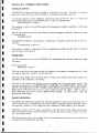
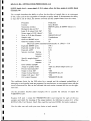
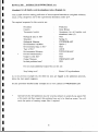
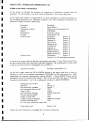
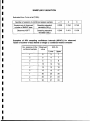
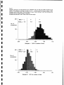
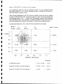
Institute of
Rreshwater
Ecology
Pnctical Sessions on RIVPACS ID+
A series of step-by-step exercises to demonstrate some of the
major options available in RIVPACS III+.
by R T Clarke, M T Furse, J F Wright & K L Symes
CONTENTS
Installing RIVPACS III+
1. Interactive predictions
la)
lb)
lc)
Id)
le)
If)
lg)
BMWP family level : manual data input
BMWP family level : data input from files
BMWP family level : 0-E input from files, assign to quality bands
BMWP family level : manual 0-E input, allow for sample bias
Abundance for all families and the abundance index
Multiple taxonomic levels (andlor seasons) on a single run
Setting up and using a customisation
2. Interactive sample comparisons
2a) Compare : manual 0 - E input, differences in O/E and quality band
2b) Compare : 0-E input from files, allow for sample biases
3. Interactive classification
4. Setting up and using defaults files
5. Batch mode operation
5a)
5b)
5c)
Using the batch setup menu option
Running a simple batch mode prediction
Multiple predictions in batch mode
6. Bias file setup
7. Quality bands file setup
RIVPACS
m+ : INTRODUC'rORY NOTES
Loading the software
The RIVPACS software should be loaded in a directory of its own. This does not prevent
input and output files being stored elsewhere if necessary (see later exercises).
To load the software, the PC should be switched on and set at the C: drive. To create the
required directory for carrying RIVPACS HI+, at the C:> prompt type
MD RIVPAC3P <<enter>>
The symbols << and >> are used throughout this document to signify a single key which must
be pressed.
The PC should now be set to the new directory before loading the software. Therefore, at the
C:> prompt type
CD RIVPAC3P
The RIVPACS software is provided on a single disk. To load it, insert the disk in drive A:
and type
A:\INSTALLR <<enter>>
The software, which is compressed, will be expanded and loaded and the state of progress
will be shown on the screen.
Your PC should now be set at the C:RIVPAC3P> prompt and the software loaded and ready
for action.
To get going type
RIVPACS <<enter>>
The first screen is the title page and this is followed by two pages of background text. Each
is exited by pressing <<enter>> or any other key.
The main menu panel offers the basic choice of type of run and the seven main options are
described in this collection of exercises.
For each of the exercises that follow you need to select one of the main panel options. The
exercises successively cover PREDICTION, COMPARE, CLASSIFICATION, DEFAULTS
SETUP, AUTOIBATCH SETUP, SAMPLE BIAS SETUP and QUALITY BAND SETUP.
HELP boxes with informative text are a menu option at many key stages. EXIT is used to
leave RIVPACS and return to the C:\RIVPAC3P> prompt. At each exercise select the
appropriate menu option.
Genela1 considerations
Throughout the following exercises the selected response to each on-screen prompt box or
menu is determined by highlighting your chosen option, using the upldown, lefdright arrows,
and pressing <<enter>> or by typing the option number or initial letter of your selection.
Sometimes <<Esc>> can be used to terminate a run and return to the initial main menu.
Many prompt boxeslmenus offer the option to return to previous screens or return to the start
(i.e. main menu panel)
Most prompt boxes allow only a single choice to be made but more than one taxonomic level
or season can be selected for each run.
IUVPACS II1+ : INTERACTIVE PREDICTIONS ( l a )
Introductolv note
Many keyboard operations are common to all RIVPACS III+ runs and are tedious to repeat
throughout this primer. They are given in italics in this first example only and are assumed
for subsequent exercises.
Pressing <<enter>> is not necessary if the initial letter of your chosen option or its menu
number is used to select it.
BMWP familv level
- manual data inout (Example la)
As a simple, introductory example, make the following choices:
<<enter>>
Procedure
Prediction
Country
Great Britain
<<enter>>
Taxonomic level(s)
BMWP families & BMWP indices (1)
<<enter>>
The C: SELECTION COMPLETED bar is now highlighted
Press <<C>>or <<enter>>
Biological data on file?
NO
<<enter>>
File input of 0 - E values?
:
NO
<<enten>
Screen input of 0 - E values? :
NO
<<enter>>
Season (s)
Spring, summer & autumn combined (7) <<enter>>
The C: SELECTION COMPLETED bar is now highlighted
Press <<C>>or <enter>>
Environmental variables
Option 1
<enter>>
Continue/Previous screen
:
Continue
<enter>>
Environmental data on file? :
NO
<<enter>>
Proceed automatically?
NO
<<enter>>
[the environmental data to be manually entered]
Predicted taxa on screen?
:
YES
<<enter>>
Outputs to disk file?
NO to each option
<<entee> d t e r each response
[in this run see taxa and scores on screen]
Stop listing taxa?
Keep it as 0.1 % for BMWP level
<enter>>
Continue/Previous screen
:
Continue
<enter>>
Now enter the following data (1 site only).
Site reference
Grid reference
Altitude (m)
Distance from source (km)
Water width (m)
Water depth (cm)
Discharge category
Boulders (% cover)
Gravel (% cover)
Sand (% cover)
Silt (% cover)
Alkalinity (mg l ~ CaCO,)
'
Slope (m km-')
Are environmental data correct?
Enter data for another site?
Environmental data are then displayed
Probabilities of group membership are given
Predicted BMWP families are listed
BMWP index values are presented
Frome at East Stoke
SY 866 867
13
43
18
64
6
13
61
22
4
172
10
Y (YES)
N (NO)
<<enter>>
<<enteo>
<<enter>>
<<enter>>
Press <<enter>> to scroll through the list
Press <<enter>> to return to the main panel
RIVPACS HI+ : INTERACTIVE PREDICTIONS ( l b )
BMWP family level
- data input fmm files (Example l b )
Initially, we offer a straightforward example to familiarise you with the use of inputloutput
files and confidence limits for OIE values.
This can be followed by examples of your own using different responses at each asterisk (*).
The responses for this exercise are as follows:
*
Procedure
Country
*
Taxonomic level(s)
Biological data on file?
Season(s)
*
Biological file name
Environmental variables
*
Environmental data on file? :
Type of file
*
Environmental filename
Allow for sample bias?
Assign to quality bands
Proceed automatically?
Output to disk file?
Output listing filename
Include predicted taxa?
*
Do not create additional output files on this run
*
Stop listing taxa?
Prediction
Great Britain
BMWP family & BMWP indices ( I )
YES
Spring, summer & autumn combined (7)
TSTFAMGB.ASC
Option 1
YES
ASCII
TSTENVGB.ASC
NO
NO
YES
YES
WKBMWPlB.LST
YES
0.1%
The three Great Britain test file sites are flagged as the prediction proceeds,
before the main panel reappears.
Examine your output file WKBMWPI.LST as follows:
Exit from main panel
At the prornpt C:WIVPAC3P> type
EDIT WKBMWP 1.LST <<enter>>
To close the DOS editor press the following three keys in sequence
<<Alt>> <<F>> <<X>>
Then re-enter RIVPACS from the C:\RIVPAC3P> prompt, type
RIVPACS <<enter>>
Now do another run and make your own choice at e x h asterisk. When making your own
choices, refer to the list of example input files in Appendix 3 of the RIVPACS III+ manual
to be sure of entering the correct file names.
RIVPACS III+ : LNTEKACTIVE PREDICTIONS ( l c )
BMWP familv level
- file input 0 - E values. assipn samples to auditv bands (Example lc)
This example introduces the option to use previously calculated observed(0) and expected(E)
BMWP index values for the samples as an input file and the facility to assign samples
probabilistically to quality bands. The 0 - E file to be used as input in RIVPACS III+ could
have been derived as an output file from a run of RIVPACS 111 which used the biological and
environmental data files for the samples.
Use the procedure detailed under example (Ib) to view the contents of 0 - E input file
TSTOET2.DAT to be used in this example.
Procedure
Country
Taxonomic level(s)
Biological data on file?
Input 0 - E values from file? :
0 - E input data filename
:
Allow for sample bias?
Assign to quality bands
Proceed automatically?
Output to disk file?
Output listing filename
:
Output 0 - E type 1 file?
Prediction
Great Britain
BMWP family & BMWP indices (1)
NO
YES
TSTOET2.DAT
No
YES use default GQA limits (2)
NO
YES
WKBMWP1C.LST
NO
The confidence limits for the OIE ratios for a sample and the subsequent estimated
probabilities of belonging to each quality band are presented, for convenience, on one output
screen. As the band given to a sample based on the GQA banding system is the lower of its
bands based on each of OIE for number of taxa and ASPT, no information is given for OIE
based on BMWP score.
Use the procedure detailed under example (lb) to view the contents of output file
WKBMWP1C.LST
KMWP familv level - screen input of 0 - E values, allow for bias. assien to aualitv bands
(Example i d )
This example introduces the ability to allow for the effect of sample bias on an assessment
of OIE values and on the assignment of samples to quality bands. It demonstrates the abiltty
to input the 0 and E values, the seasons involved and the sample biases from the screen.
Procedure
Country
Taxonomic level(s)
Biological data on file?
Input 0 - E values from file? :
Screen input of 0 - E values? :
Store in 0 - E data filename :
Sample code
Observed BMWP score
:
Observed number of taxa
Observed ASPT calculated
Expected BMWP score
Expected number of taxa
:
Expected ASPT
Seasons involved Spring :
Summer :
Autumn :
Specify sample biases?
Bias for
Summer :
Autumn :
Enter another sample?
Assign to quality bands
Proceed automatically?
Output to disk file?
Output listing filename
Output 0 - E type I file?
:
0 - E output filename
Prediction
Great Britain
BMWP family & BMWP indices (1)
NO
NO
YES
WKOETID.DAT
Tumbledown
139
25
automatically as 139/25 = 5.56
190.1
30.2
6.29
N
Y
Y
Y
1.9
2.4
N
YES use default GQA limits (2)
NO
YES
WKBMWP1D.LST
YES
WKBMWPI D.OE1
The confidence limits for the O/E ratios for a sample and the estimated probabilities of
belonging to each quality band are presented, for convenience, on one output screen with the
results uncorrected for bias on the left-hand side and results corrected for bias on the righthand side.
Use the procedure detailed under example (Ib) to examine the contents of output file
WKBMWPI D.LST.
Examine 0 - E type 1 output file WKBMWPlC.OE1 (one long line for each of the two
samples) and check the meaning of the output statistics by referring to section 6.11 of the
RIVPACS III+ User Manual. (Such files could be read into EXCEL for further analysis.)
Now do other runs and make your own choice at each asterisk
RIVPACS III+
INTERACTIVE PREDICTIONS ( l e )
Abundance for all families and the abundance index (Examole l e )
This example involves making predictions of mean expected abundances (weighted arithmetic
means of log categories) and of the experimental abundance index 414.
The required responses for this exercise are:
Procedure
Country
Taxonomic level(s)
Biological data on file?
*
Biological filename
Environmental variables
Environmental data on file?
Type of file?
Environmental filename
Proceed automatically?
Output to disk file?
Output filename
Include predicted taxa?
Prediction
Great Britain
Abundance for all families and
abundance index (2)
YES
Spring (1)
TSTSPRGB.ASC
Option 1
YES
ASCII
TSTENVGB.ASC
YES
YES
WKSPABUN.LST
YES
Do not create additional output files on this run
Stop listing taxa?
Retain 0.0 log abundance.
As in the previous example (b), the three test sites are flagged as the prediction proceeds,
before the main panel reappears.
Use the procedure detailed under example (b) to view contents of WKSPABUN.LST
*
Alternatively the full prediction may be viewed at leisure on screen if you answer NO
at this point and then request that predicted taxa are to be listed on screen. You still
retain the option of creating output files if required.
Multiple taxonomic levels (andlor seasons) on a single tun (Exam~lei f )
In theory it is possible to request predictions at 5 taxonomic levels (1-5) and for 7
seasonslseasonal combinations (1-7). However, when using BMWP families and indices
(taxonomic level I ) with error assessment, no other taxonomic level should be selected. Also,
we recommend that you exclude taxonomic level 5 (Existing customisation) until you have
become familiar with this option (see next section on setting up a customisation).
Merely excluding taxonomic levels 1 and 5 could still generate 17 predictions for each site
if you request all of taxonomic levels 2-4 and seasons 1-7 (NB taxonomic level 2, abundance
for all families only operates on seasons 1-3 (i.e. single seasons) at present).
Hence, we suggest that you are selective in your initial choice. Bear in mind that there are
3 sites i n the environmental data example files and that if you request output files they will
be substantial if you ask for the inclusion of predicted taxa.
As one example, try the following:
Procedure
Country
Taxonomic level(s)
Biological data on file?
Season(s)
Environmental variables
Environmental data on file? :
Type of file
Environmental filename
Proceed automatically?
Output to disk file?
Output biological filename :
Include predicted taxa?
Do not create additional output files
Stop listing taxa?
Prediction
Great Britain
Choose 3 & 4
NO - on this initial run.
[ On a later run, reply YES, but bear in
mind the need to input the appropriate
example files when requested]
Choose 1 & 7
Option I
YES
ASCII
TSTENVGB.ASC
YES
YES
WKSPMULT.LST
YES
Retain as 0.1 for all families
Change to 50.0 for species
Follow the previous instructions for example (b) to examine the output file.
For each of the 3 example sites, the output sequence is,
Site namelcode
Environmental data
Probabilities of group membership
Predicted families
Spring
Spring, summer and autumn combined
Predicted species
Spring
Spring, summer and autumn combined
To
To
To
To
0.1%
0.1%
50.0%
50.0%
RNPACS
-
III+ : INTERACTIVE PREDICTIONS (ld
Settinp u~ and using a customisation.
I
At the outset, go through the sequence of operations to familiarise yourself with the
procedure. Do not attempt to set up a useful customisation. This can be done later.
I
In the simple (and unlikely!) example below, we want a prediction in which all members of
the Tricladida (flatworms) are identified at generic level. The remaining invertebrates are
predicted at major taxonomic group only.
Procedure
Country
Taxonomic level(s)
Name?
Description?
Country
Current taxon
Prediction
Great Britain
Chose new customisation (6)
CUSTOM 1
Triclads to genus
Great Britain (G)
Tricladida.
Select? N
Planariidae.
Select? N
Planan'a sp.
Select? Y
Polycelis sp.
Select? Y
Phugocata sp.
Select? Y
Crenobiu sp.
Select? Y
Dugesiu sp.
Select? Y
Dendrocoelidae
Select? N
Bdellocephala sp.
Select? Y
Dendrocoelum sp.
Select? Y
Gastropoda
Select? Y
Answer Y to all subsequent questions
Current taxon
1
I
1
I
At the end, the screen indicates that this customisation generates 3 1 taxa. The necessary files
are then created before the taxonomic level panel reappears. The customisation is thus saved
to file and can be accessed in subsequent runs as follows:
Existing customisation ( 5 )
Taxonomic level(s)
On the next screen choose the UP or DOWN options in the upper menu box as often as
necessary to scroll to the required customisation (CUSTOMI) in the lower menu box. After
highlighting the required customisation, choose SELECT. Choose SELECT again on the
subsequent screen to re-enforce your choice. [This screen also offers the option of deleting
unwanted customisations. Use it on a subsequent occasion to delete CUSTOMI ]
Biological data on file?
NO
Season(s)
Spring ( 1 )
Environmental variables
Option I
Environmental data on file? :
YES
Type of file?
ASCII
Environmental filename
TSTENVGB.ASC
Proceed automatically?
YES
Output to disk file?
YES
WKSPCUST.BI0
Output biological filename :
Include predicted taxa?
YES
Do not create additional output files
I
I
Stop listing taxa?
Retain 0.1 %
Follow prevlous instructions in example (b) to examine output file.
8
RIVPACS HI+ : INTERACTIVE COMPARE (2al
Cornoam two sarnoles - screen inout of 0 - E values. assess differences in OIE values and
likelihood of differences in aualitv bands (Examole 2 4
This example introduces main menu procedure Compare. This is used to compare two samples
(or multiple pairs of samples) by assessing the statistical significance of the differences in
their OIE values and by assessing the likelihood of a difference in quality bands.
The two samples can be the same site at different times, or two different sites; the season(s)
involved can be the same or different. The only information needed for each sample is:
the previously calculated observed(0) and expected(E) values of BMWP score,
number of taxa and ASPT for the two samples.
( i i ) the seasons involved
(iii) the sample biases applicable to each season involved (optional)
(iv) whether the expected values of both samples were based on the same values of the
environmental variables.
(i)
In this example, the information is input from the screen; in later examples it is read from
files.
Procedure
Input 0 - E values from file? :
*
Store in 0 - E data filename :
*
Sample code
3
Observed BMWP score
:
*
Observed number of taxa
Observed ASPT calculated automatically as:
*
Expected BMWP score
*
Expected number of taxa
:
*
Expected ASPT
*
Seasons involved Spring :
*
Summer
%
Autumn :
*
Specify sample biases?
*
Bias for
Summer
*
Autumn
*
Enter another sample?
:
*
Same values for variables
Assign to quality bands
*
Proceed automatically?
Output to disk file?
Output listing filename
*
Tables of change in band
:
Output 0 - E type 1 file?
Output 0 - E type 2 file?
Compare
NO
WKOET2A.DAT
Pickmeup Place
Tumbledown
139
83
25
17
83/17 = 4.88
139i25 = 5.56
190.1
175.6
30.2
27.1
6.29
6.48
N
N
Y
Y
Y
N
Y
1.9
2.5
2.4
N
N
YES use default GQA limits (2)
NO
YES
WKCOMP2A.LST
Taxa, ASPT and Overall table
No
No
The assessment of the OIE values and probabilistic banding for each of the two individual
samples is given first; this part of the output to the screen andlor listing file and 0 - E type 1
file is exactly the same as for procedure Prediction for the individual samples. Next is a
statistical assessment for differences in O/E values between the two samples and finally an
assessment of the likelihood of differences in quality band when based on O/E for number
of taxa, ASPT or the overall GQA band.
Use the procedure detailed under example (Ib) to view the contents of 0 - E input file
WKOET2A.DAT made from the screen input and the output listing file WKCOMP2A.LST.
KIVPACS III+ : Ih'TEKACTIVE COMPARE (2b)
Compare two samples - file input of 0 - E values. assess differences in OIE values and
likelihood of differences in aualitv bands both ignoring- and corrected for sample biases
(Examole 2bl
This example demonstrates the potential effect of allowing for sample biases in the
comparison of two samples. The observed(0) and expected(E) values for the samples are also
read from an 0 - E input file; this input file could have been derived as an output file, from
a previous run of RIVPACS Ill+ or RIVPACS 111, based on the biological and environmental
data files for the samples.
Use the procedure detailed under example (lb) to view the contents of 0 - E input file
TSTOET2.DAT to be used in this example.
*
*
*
*
*
*
Procedure
Input 0 - E values from file?
Single or pair of files
0 - E input data filename
Same values for variables
Allow for sample bias?
Obtain biases from?
Bias filename
Assign to quality bands
Proceed automatically?
Output to disk file?
Output listing filename
Tables of change in band
Output 0 - E type 1 file?
0 - E type 1 output filename
Output 0 - E type 2 file?
0 - E type 1 output filename
:
Compare
YES
1
:
:
:
:
:
:
TSTOET2.DAT
No
YES
bias file ( I )
TSTBIAS.DAT
YES use default GQA limits (2)
NO
YES
WKCOMP2B.LST
Overall table only
Yes
WKCOMP2B.OE 1
Yes
WKCOMP2B.OE2
When correction for sample bias is requested all assessments are first given uncorrected for
bias and then corrected for bias.
The assessment of the OIE values and probabilistic banding for each of the two individual
samples is given first; this part of the output to the screen andlor listing file and 0 - E type I
file is exactly the same as for procedure Prediction for the individual samples. Next is a
statistical assessment for differences in O/E values between the two samples. The assessment
of the likelihood of differences in quality band is given in a sequence of output screens based
on (in order) O/E for number of taxa, ASPT or the overall GQA band, uncorrected for bias,
then corrected for bias.
Use the procedure detailed under example ( l b ) to view the contents of output listing file
WKBMWP2B.LST
Examine 0 - E type I output file WKBMWP2B.OEI (one long line for each of the two
samples) and 0 - E type 2 output file WKCOMP2B.OE2 (one long line for sample comparison
statistics ignoring bias and a second corrected for bias). Check the meaning of the output
statistics in both files by referring to sections 6.1 I and 6.12 of the RIVPACS III+ User
Manual. (Such files could be read into EXCEL for further analysis).
RIVPACS III+ : INTERACTIVE BIOLOGICAL CLASSIFICATlON (3)
Soecies level classification
The classification procedures are simple to operate and depend upon the biological data being
held on file. Only one practical example is given here.
A new site may only be classified using species level data (three seasons combined) or
BMWP family data (three seasons combined).
Bear in mind that when the reference sites were used to develop the 35 group Great Britain
and seven group Northern Ireland classifications, information on both species composition and
family abundances was utilised. Use of this same procedure for classification of new sites
would have been very cumbersome and is unlikely to have been used in practice. The
simplified options of species or BMWP family classification have, thus, been retained from
RIVPACS 11.
We recommend that classification results are used, with caution, to allocate sites to a
restricted area of the classification. It is unwise to place great importance to the individual
classification group with which the site has most in common.
As an example, use the following procedure:
Procedure
Country
Taxonomic level
Type of file?
Biological filename
Output to disk file?
Proceed automatically?
Then view the results on screen,
Biological classification
Great Britain
Species
ASCII
TSTSPRGB.ASC
NO
NO
RlVPACS LII+ : DEFAULTS FILES (4al
Using defaults files
Defa~~lts
files contain the paths for the user's input and output files
At installation, the RIVPACS III+ program is instructed to find all of the input files (eg the
example environmental and biological files) in the RIVPACS III+ software directory and all
output files are initially written to this directory. RIVPACS III+ is supplied with a main
"defaults" file entitled DEFAULTS.DAT which contains this instruction.
The user may make alternative defaults files, if required, instructing the program to input and
output files to alternative directories or sub-directories. This example shows how defaults files
are created and used.
In this exercise you will:
i)
ii)
iii)
iv)
create a new directory and suitable sub-directories for holding input and output files
place example environmental and biological files in the input sub-directories
use the input files in a prediction
examine the results in the new output sub-directory
Creating directories and sub-directolies
Exit RIVPACS at the main panel
Return to the main C:> prompt by typing CD.. <<enter>>
Create a directory called RUBBISH by typing MD RUBBISH <<enter>>
Move to your new directory by typing CD RUBBISH <<enter>>
Create six new sub-directories (BIO, ENV and OUT) by typing
MD
MD
MD
MD
MD
MD
BIO <<enter>>
ENV <<enter>>
OEl <<enter>>
BIAS <<enter>>
BAND <<enter>>
OUT <<enter>>
Put example input files in the new sub-directories
Whilst at the existing prompt of C:\RUBBISH>, type
COPY C:\RIVPAC3P\TSTENVGB.ASC
C:\RUBBISH\ENV
This copies a test file of environmental data to sub-directory C:\RUBBISH\ENV
Whilst at the existing prompt of C:\RUBBISH>, type
COPY C:\RIVPAC3P\TSTFAMGB,ASC C:\RUBBISH\BIO
This copies a test file of family level biological data to sub-directory C:\RUBBISH\BIO
Similarly, whilst at the existing prompt of C:\RUBBISH>, type
COPY C:\RIVPAC3P\TSTOET2.DAT C:\RUBBISH\OEI
COPY C:\RIVPAC3P\TSTBIAS,DAT C:\RUBBISH\BIAS
COPY C:\RIVPAC3P\TSTBAND.DAT C:\RUBBISH\BAND
RIVPACS I l l + : DEFAULTS FILES (4b)
Returning to RIVPACS Kl+
At the prompt C:\RUBBISH> type CD C:\RIVPAC3P <<enter>>
At the prompt C:\RIVPAC3P> type RIVPACS <<enter>>
Creatin~a new defaults file
In RIVPACS III+ select Defaults setup from the main panel
The screen shows a series of questions which must be answered successively by typing the
necessary information in screen boxes. In this example the following actions are required:
The first screen box appears with the file name DEFAULTS.DAT already entered. Enter the
new defaults file name by over-typing
DEF3.DAT <<enter>>
The next screen box highlights the instruction E: Edit this file. Select this option by pressing
either <<enten> or <<E>>.
A new screen is now displayed
The next two screen boxes allow the input paths to be entered for the biological and
environmental data respectively. Type the following
C:\RUBBISH\BIO <<enter>> (The input path for the biological data)
C:\RUBBISH\ENV <<enter>> (The input path for the environmental data)
C:\RUBBISH\OEI <<enter>> (The input path for the 0 - E data)
C:\RUBBISH\BIAS <<enter>> (The input path for the sample bias file)
C:\RUBBISH\BAND <<enter>> (The input path for the quality band limit file)
The next box allows the output path to be defined. Type the following
Press <<enter>> again to move on to the next screen
At the next box type Y <<enter>> to initiate the saving of the file.
The next box displays your chosen defaults file name, DEF3.DAT
Type <<enter>> to confirm this.
You will be asked if you want to overwrite the existing file. In this exercise respond YES.
This prompt is a useful reminder to ensure you don't lose an existing file which you want to
keep.
Now press <<F3>> in order to save the file.
RlVPACS ILL+ : DEFAULTS FILES (4cl
select in^ a defaults file
In order to use your new defaults file i n interactive mode you first need to select it as follow.;:
Select Defaults setup at the main panel
In the first screen box, replace DEFAULTS.DAT as the defaults file name, by typing
DEF3.DAT
At the next screen box either
Select U: Use as defaults file by pressing <<enter>>,
Either option automatically returns you to the main panel.
or
Press <<Uz>
Your new defaults file is set and you can proceed with whatever procedure run you require.
[Jsinp
-
vour defaults file
Having created and selected your new defaults file, DEF3.DAT, try the following exercise
which uses biological and environmental data only from file.
Make a simple family level prediction for Great Britain by choosing option 1 from the
taxonomic selection menu and option 7, spring, summer and autumn, from the season menu.
Select the options that state that you hold environmental data on file in ASCII format.
When requested, give the appropriate biological and environmental file names.
Biological filename
Environmental filename
TSTFAMGB.ASC
TSTENVGB.ASC
Your defaults file, DEF3.DAT, will find these files for you using the paths you have
stipulated.
When prompted, request that the prediction proceeds automatically without user intervention.
When requested send the results, including the probabilities of taxon occurrences, to output
file WKSPDFIL.LST
Your defaults file will automatically send this to the required sub-directory
To see the contents of the output file exit RIVPAC3P at the main panel and type:
EDIT C:\RUBBISH\OUT\WKSPDFIL.LST
Further information
After exiting RIVPACS III+, the next use of the system will automatically revert to using
DEFAULTS.DAT as the defaults file.
If you wish to use DEF3.DAT again it needs to be re-selected using the procedure above. If
you want to change the defaults directory semi-permanently, then you must edit the file
DEFAULTS.DAT as required.
For a fuller explanation of the defaults file procedures it is important to study section 2.5 of
the RIVPACS III+ Manual.
KIVPACS IU+ : BATCH MODE (5a)
Thc making, use and format of batch files is described in the Sections 2.6, 2.9.3 and 6.2 of
the RIVPACS IIIt- User Manual.
us in^ the AutolBatch setup menu o ~ t i o n(Examole 5al
At the main panel choose Auto/Batch setup. Type in the following responses:
Batch file name
Edit batch instructions set number
Edit or delete this set
Defaults file name
Procedure
Country
Taxonomic level(s)
Biological data files?
Season(s)
Predictive variables
Biological filename
Environmental file format
Environmental filename
Allow for sample bias?
Bias filename
Assign to quality bands
Output listing file
Include predicted taxa?
Stop listing taxa at % probability?
Additional output files
Environmental data
BMWP 0 - E type 1
Overwrite existing files?
Save changes?
NEWAUTO.DAT
1 (first instruction set of new file)
E (to allow entry of new instructions)
DEFAULTS.DAT
[This means that the input and outpi~t
files will be in the same directory as the
RIVPACS III+ software]
Prediction (1)
Great Britain (1)
BMWP families (1)
YES (Y)
All three seasons combined (7)
Option 1
TSTFAMGB.ASC
ASCII (1)
TSTENVGB.ASC
I: Yes (fixed)
TSTBIAS.DAT
I: Yes (use EA GQA defaults)
WKBATCHI .LST
Y
0.1%
WKBATCHl .ENV
WKBATCHI .OE1
YES (Y)
YES (Y), to file NEWAUTO.DA1
Press <<F3>> to save the batch file and to return to the main panel.
Exit the main panel and use the procedure detailed under example (lb) to view the contents
of batch file NEWAUTO.DAT created above. The file includes the batch mode instruction
line and a list of the specified files.
Runnin~a simole batch mode orediction
To run RIVPACS III+ in batch mode, at the C:\RIVPAC3P> prompt type
RIVPACS AUTO NEWAUTO.DAT <<enter;.>
The program only displays the name of the sample(sj currently being processed
On completion of the batch run, examine the various output files, of the form
WKBATCHI.***, using the procedure detailed under example (lb).
Multiple runs in batch mode (Example 5bl
This example runs a prediction using 0 - E input files, then runs a comparison using the output
0 - E type I file for the three samples i n example 5a with the first three samples i n another OE input file called TSTOETI .DAT.
Procedure
AutoIBatch setup
Batch file name
MULTAUTO.DAT
Edit batch instructions set number :
1
Edit or delete this set
E
DEFAULTS.DAT
Defaults file name
Procedure
Prediction (1)
Country
Great Britain (1)
BMWP families ( I )
Taxonomic level(s)
Biological data files?
N
0 - E type 1 file as input?
Y
0 - E type 1 input filename
TSTOET2.DAT
Allow for sample bias?
1: Yes (fixed)
TSTBIAS.DAT
Bias filename
Assign to quality bands
2: No
WKBATCH2.LST
Output listing file
Additional output files
BMWP 0 - E type 1
WKBATCH2.0E I
Overwrite existing files?
YES (Y)
Save changes?
YES (Y), to file MULTAUTO.DAT
Press <<F3>> to save the batch file and return to the main panel.
AutolBatch setup
Procedure
MULTAUTO.DAT
Batch file name
Edit batch instructions set number :
2
Edit or delete this set
E
DEFAULTS.DAT
Defaults file name
Procedure
Compare (2)
2
No. of files containing 0 - E values :
N
Same values of variables
0 - E filename for samples A
W KBATCH 1.OE l
0 - E filename for samples A
TSTOETI .DAT
Allow for sample bias?
I : Yes (fixed)
TSTBIAS.DAT
Bias filename
Assign to quality bands
I: Yes (use EA GQA defaults)
Output listing file
WKBATCH3.LST
Tables of change i n band
Overall table only
Additional output files
BMWP 0 - E type 1
WKBATCH3.0EI
BMWP 0 - E type 2
WKBATCH3.0E2
Overwrite existing files?
YES (Y)
Save changes?
YES (Y), to file MULTAUTO.DAT
Press <<F3>> to save the batch file and return to the main panel.
Now run MULTAUTO.DAT from the C:\RIVPAC3P> prompt by typing
RIVPACS AUTO MULTAUTO.DAT <<enter>>
After the batch run, examine the output files as directed previously
Batch files can also be used to run classifications or a mixed package of both predictions,
comparisons and classifications. Defaults files other than the standard DEFAULTS.DAT can
be used to input and output files from and to other directories.
Try some other examples.
RIVI'ACS IU+ : SAMPLE BIAS FILE SETUP (6)
To allow for sample bias, RIVPACS requires an appropriate estimate of the average bias for
single season samples from each of the three RIVPACS seasons. In interactive runs of
RIVPACS samples, these biases can either be entered from the screen, or read from a sample
bias file. In batch mode, the biases must be read from a sample bias file.
The format of bias files is described in Section 6.9 of the RIVPACS III+ User Manual
A bias file could be made using an ASCII file editor (such as EDIT in MS-DOS)
This example demonstrates how to make a sample bias file using the sample bias setup option
of interactive RIVPACS. The bias file will contain biases for each pair of samples (A and B)
to be compared using RIVPACS procedure Compare. However, this bias file can also be used
in RIVPACS prediction runs; in which case all the samples are assumed to have the biases
specified for samples A.
Using the Sample bias setuo menu option (Examole 6)
Procedure
Bias filename
Single or Paired samples
Sample A bias for : Spring
Summer
Autumn
Sample B bias for : Spring
Summer
Autumn
Sample bias setup
WKBIAS.DAT
2 (paired)
2.7
2.3
2.1
1.9
1.9
1.7
Save changes?
YES (Y), to file WKBIAS.DAT
Press <<F3>> to save the batch file and return to the main panel
RIVI'ACS IlI+ : OUALITY B A N D FILE SETUP (7)
'1.0 assign samples to quality bands, RIVPACS requires the lower limit of OIE for each baritl
for each of BMWP score, number of taxa and ASPT. In interactive runs of RIVPACS
samples, the band lower limits can either be entered from the screen, or read from a quality
band file. In batch mode, the limits must be read from a quality band file.
The format of quality band files is described in Section 6.10 of the RIVPACS III+ User
Manual.
A quality band file could be made using an ASCII file editor (such as EDIT in MS-DOS)
This example demonstrates how to make a quality band file using the Quality band setup
option of interactive RIVPACS.
Usine
-
the Ouditv band setup menu ootion (Examole 7)
Procedure
Quality band setup
WKBAND.DAT
Bias filename
Number of bands
4
Name for first band
Fine
Score O/E
:
0.80
Lower limit for :
0.85
Taxa OIE
0.90
ASPT OIE :
Name for second band
Good
Score OIE
:
0.60
Lower limit for :
:
0.70
Taxa OIE
ASPT OIE
:
0.80
Name for third band
Fair
Score OIE
:
0.40
Lower limit for :
:
0.55
Taxa OIE
ASPT OIE :
0.70
Name for fourth band
Poor
Lower limits,for La~thand are automatically set to 0.00
Save changes?
YES (Y), to file WKBAND.DAT
Press c<F3>> to save the batch file and return to the main panel.
STATISTICAL NOTES ON METHODS USED
TO ASSESS ERRORS IN O/E MEASURES OF
BIOLOGICAL QUALITY
RIVPACS Ill+
STATISTICAL METHODS USED TO ASSESS ERRORS
IN O/E MEASURES OF BIOLOGICAL QUALITY
Details of exact procedures are given in Section 7 of the RIVPACS
Ill+ User Manual.
Background research in :
Furse, M.T., Clarke, R.T., Winder, J.M., Symes, K.L., Blackbum, J.H., Grieve, N J. &
Gunn, R.J.M.(1995).
Biological assessment methods: c o n t r o the
~ quality of biological data. package 1:
The variability of data used for assessing the biological condition of rivers.
Final report to the National Rivers Authority. R&D Note 412. 114 pp.
BMWP indices : ASPT, number of taxa and BMWP score
0 = Actual or 'face' value of OBSERVED BMWP index for sample
E = Actual EXPECTED BMWP index value for the sample
Index of biological quality
=
Q
=
OIE
Computer simulation of possible values of OIE for the sample
based on estimates of :
(i)
typical sampling variation
(ii) sample sorting and identification errors
(iii) errors in the values of the environmental predictor variables
Frequency distribution of simulated values provides confidence
limits for the sample's OIE index of quality
SAMPLING VARIATION
Estimatedfrom Furse et al (1995) :
-> 1
2
3
Sampling standard
deviation (SDq6~)
0.228
0.164
0.145
Sampling standard
deviation (SDA)
0.249
0.161
0.139
Number of seasons in combined season sample
Square root of observed
number of BMWP taxa
Observed ASPT
Examples of 95% sampling confidence intervals (95%CL) for observed
values of number of taxa based on single or combined season samples
SAMPLE SORTING AND IDENTIFICATION ERRORS
Results derived from Furse et al (1995) analyses of sample audit data:
Bias = Net underestimation of number of taxa in the sample
= Net "gains"estimated from a quality control procedure or audit scheme
Assume a Poisson distribution for the sample bias
Poisson distributbn of sample
biases when average bias is 2.0
Need to specify B1, B2 and B3, the average biases for each of
spring, summer and autumn single season samples
Average bias for a two seasons combined sample
51% (sum of the biases in the two individuals seasons)
Average bias for a three seasons combined sample
37% (sum of the biases in the three individuals seasons)
ERRORS IN THE EXPECTED (E) VALUES
DUE TO ERRORS IN MEASURING THE ENVIRONMENTAL
PREDICTOR VARIABLES
Remember : ALL RIVPACS predictions must be based on the average values
of the environmental variables measured in each of the three RIVPACS
seasons. Ideally they should be the average of several years three season
averages.
Results derived by Furse et al(1995):
Size of error in E values does not depend significantly on either :
the number of seasons involved in the biological sample
(i)
or
(ii)
the type of site
Estimates are :
Standard deviation for Expected number of taxa
Standard deviation for Expected ASPT
-
0.53
0.081
Note : may under-estimate size of errors in the Expected value, especially for
long-term average predictions
GENERATING THE SIMULATED VALUES OF OIE
Q,
=
OIE for r'h simulation =
0
RO
B
=
--
Actual OBSERVED value
random element of sampling variation
random Poisson bias term
E
RE
-
Actual EXPECTED value
random variation due to errors in values for environmental variables
O + R -o- + B
E +RE
COMPARING TWO SAMPLES
Q,, and
D,
-
Qn denote the OIE values for samples 1 and 2
(or samples A and 6)for the thsimulation
Qa
-
Q,, = difference in OIE values for the thsimulation
Frequency distribution and confidence limits for D, indicate whether the OIE
values for the hnro samples are statistically significantly different.
Figure I:
Frequency histogram of 1000 RIVPACS III+ simulated values of 0E for number of taxa for two
samples. The histogram is divided into bands (A, B, C,. ..) based on the Environment Agency's GQA
biological quality band system. The percentage of values (%prob) falling in each band estimates the
probability that the sample belongs to each band.
X denotes the o b s e ~ e dor 'face' value of OIE for each sample
No. of
simulations
Sample A : OIE for number of taxa
No. of
simulations
.
I
I
I
I
I
0.55
0.70
0.55
1.00
1.15
Sample B : OIE for number of taxa
1
I
I
I
I
Figure 2: RIVPACS Ill+ conlparison of two samples
Cross-classification table showing the probability sample A is in one biological quality
band whilst sample B in is in another (perhaps the same or different) band based on
their O E values for number of taxa
Table plots the distribution of the O E values for number of taxa for the two samples
for each of 1000 RIVPACS III+ simulations (shown as dots). The plot is divided into
cells denoting bands (A, B, C,. . .) based on the Environment Agency's GQA biological
quality banding system. The percentage of simulations falling in each cell of the twoway table estimates the probability that samples A and B have the indicated bands.
X denotes the observed or 'face' value of OIE for each of the two samples
Band -->
c
% Prob 29.7%
1.1
Sample A
-
1.o
-
69.0%
.
:.- . ..
:
a
1.3%
b
Band % Prob
.
.
.:.. .. .. . ..
a
84.9%
b
15.1%
-
.
-
0.0%
0.0%
I
0.6
.
0.7
0.0%
c
I
I
I
I
0.8
0.9
1.O
1.1
Sample B : OIE for taxa
Probability
No difference in band
=
1.3% + 10.0% =
11.3%
Sample B one band worse than Sample A
= 59.0% + 5.1% =
64.1%
Sample B two bands worse than Sample A
= 24.6%
24.6%
=
0.0%