Download P4.26 R4.25 Parallelization-with-increased-performance

Prototype P4.26, Report R4.25
Parallelization with increased performance based
on model partitioning with TLM-couplings
December, 2012
Peter Fritzson, Mahder Gebremedhin, Martin Sjölund (LIU)
•••••••••••••••••••••••••••••••••••••••••••••
This document is public.
Deliverable
OPENPROD
(ITEA 2)
Page 2 of 2
Summary
This deliverable includes two prototypes using two different approaches to parallelism, described in the
following papers. Both prototypes are implemented within OpenModelica.
 Paper 1, “A Data-Parallel Algorithmic Modelica Extension for Efficient Execution on Multi-Core Platforms”
describes a parallel extension to the algorithmic part of the Modelica. This extension is fully integrated in the
OpenModelica, and was used in a parallel programming tutorial at the Modelica conference in Munich,
December 2012. Code written in this language extension is compiled to the OpenCL parallel programming
C-style language, which is portable both to multi-core GPUs and CPUs. Speedup up to 300 for large
problems has been achieved for some applications.

Paper 2, “TLM and Parallelization”, describes a way of using transmission line modeling to partition
equation-based model, thus enabling the parts to be simulated partly in parallel. Transmission line modeling
(TLM) is a technique where the wave propagation of a signal in a medium over time can be modeled. The
propagation of this signal is limited by the time it takes for the signal to travel across the medium. By
utilizing this information it is possible to partition the system of equations in such a way that the equations
can be partitioned into independent blocks that may be simulated in parallel. This leads to improved
efficiency of simulations since it enables taking advantage of most of the full performance of multi-core
CPUs. An early prototype implementation has been developed in OpenModelica where the Modelica delay()
built-in function is used to introduce TLM-style decoupling between model parts, which is then detected by
the compiler for parallelization purposes.
Publications and Reports included in this Document
1. Mahder Gebremedhin, Afshin Hemmati Moghadam, Peter Fritzson, Kristian Stavåker. A Data-Parallel
Algorithmic Modelica Extension for Efficient Execution on Multi-Core Platforms. In Proceedings of the 9th
International Modelica Conference (Modelica'2012), Munich, Germany, Sept.3-5, 2012
2.
Martin Sjölund. TLM and Parallelization. Internal Research Report, Linköping University, December 2012.
OPENPROD
A Data-Parallel Algorithmic Modelica Extension for Efficient
Execution on Multi-Core Platforms
Mahder Gebremedhin, Afshin Hemmati Moghadam, Peter Fritzson, Kristian Stavåker
Department of Computer and Information Science
Linköping University, SE-581 83 Linköping, Sweden
{mahder.gebremedin, peter.fritzson, Kristian.stavaker}@liu.se, [email protected]
Abstract
New multi-core CPU and GPU architectures promise
high computational power at a low cost if suitable
computational algorithms can be developed. However,
parallel programming for such architectures is usually
non-portable, low-level and error-prone. To make the
computational power of new multi-core architectures
more easily available to Modelica modelers, we have
developed the ParModelica algorithmic language extension to the high-level Modelica modeling language,
together with a prototype implementation in the
OpenModelica framework. This enables the Modelica
modeler to express parallel algorithms directly at the
Modelica language level. The generated code is portable between several multi-core architectures since it is
based on the OpenCL programming model. The implementation has been evaluated on a benchmark suite
containing models with matrix multiplication, Eigen
value computation, and stationary heat conduction.
Good speedups were obtained for large problem sizes
on both multi-core CPUs and GPUs. To our
knowledge, this is the first high-performing portable
explicit parallel programming extension to Modelica.
Keywords: Parallel, Simulation, Benchmarking,
Modelica, Compiler, GPU, OpenCL, Multi-Core
1
Introduction
Models of large industrial systems are becoming increasingly complex, causing long computation time for
simulation. This makes is attractive to investigate
methods to use modern multi-core architectures to
speedup computations.
Efficient parallel execution of Modelica models has
been a research goal of our group for a long time [4],
[5], [6], [7], involving improvements both in the compilation process and in the run-time system for parallel
execution. Our previous work on compilation of dataparallel models, [7] and [8], has primarily addressed
compilation of purely equation-based Modelica models
for simulation on NVIDIA Graphic Processing Units
(GPUs). Several parallel architectures have been targeted, such as standard Intel multi-core CPUs, IBM Cell
B.E, and NVIDIA GPUs. All the implementation work
has been done in the OpenModelica compiler framework [2], which is an open-source implementation of a
Modelica compiler, simulator, and development environment. Related research on parallel numeric solvers
can for example be found in [9].
The work presented in this paper presents an algorithmic Modelica language extension called ParModelica for efficient portable explicit parallel Modelica programming. Portability is achieved based on the
OpenCL [14] standard which is available on several
multi-core architectures. ParModelica is evaluated using a benchmark test suite called Modelica PARallel
benchmark suite (MPAR) which makes use of these
language extensions and includes models which represent heavy computations.
This paper is organized as follows. Section 2 gives a
general introduction to Modelica simulation on parallel
architectures. Section 3 gives an overview of GPUs,
CUDA and OpenCL, whereas the new parallel Modelica language extensions are presented in Section 4. Section 5 briefly describes measurements using the parallel
benchmark test suite. Finally, Section 6 gives programming guidelines to use ParModelica, and Section 7
presents conclusions and future work.
2
Parallel Simulation of Modelica
Models on Multi-Core Computers
The process of compiling and simulating Modelica
models to sequential code is described e.g. in [3] and
[12]. The handling of equations is rather complex and
involves symbolic index reduction, topological sorting
according to the causal dependencies between the equations, conversion into assignment statement form, etc.
Simulation corresponds to "solving" the compiled
equation system with respect to time using a numerical
integration method.
Compiling Modelica models for efficient parallel
simulation on multi-core architectures requires additional methods compared to the typical approaches described in [3] and [12]. The parallel methods can be
roughly divided into the following three groups:
In Section 3.1 the NVIDIA GPU with its CUDA
programming model is presented as an influential example of GPU architecture, followed by the portable
OpenCL parallel programming model in Section 3.2.
 Automatic parallelization of Modelica models. Several approaches have been investigated: centralized
solver approach, distributed solver approach and
compilation of unexpanded array equations. With
the first approach the solver is run on one core and
in each time-step the computation of the equation
system is done in parallel over several cores [4]. In
the second approach the solver and the equation system are distributed across several cores [5]. With
the third approach Modelica models with array
equations are compiled unexpanded and simulated
on multi-core architectures.
 Coarse-grained explicit parallelization using components. Components of the model are simulated in
parallel partly de-coupled using time delays between the different components, see [11] for a
summary. A different solver, with different time
step, etc., can be used for each component. A related approach has been used in the xMOD tool [26].
 Explicit parallel programming language constructs.
This approach is explored in the NestStepModelica
prototype [10] and in this paper with the ParModelica language extension. Parallel extensions have
been developed for other languages, e.g. parfor loop
and gpu arrays in Matlab, Visual C++ parallel_for,
Mathematica parallelDo, etc.
An important concept in NVIDIA CUDA (Computer
Unified Device Architecture) for GPU programming is
the distinction between host and device. The host is
what executes normal programs, and the device works
as a coprocessor to the host which runs CUDA threads
by instruction from the host. This typically means that a
CPU is the host and a GPU is the device, but it is also
possible to debug CUDA programs by using the CPU
as both host and device. The host and the device are
assumed to have their own separate address spaces, the
host memory and the device memory. The host can use
the CUDA runtime API to control the device, for example to allocate memory on the device and to transfer
memory to and from the device.
3
GPU Architectures, CUDA, and
OpenCL
Graphics Processing Units (GPUs) have recently become increasingly programmable and applicable to
general purpose numeric computing. The theoretical
processing power of GPUs has in recent years far surpassed that of CPUs due to the highly parallel computing approach of GPUs.
However, to get good performance, GPU architectures should be used for simulation of models of a regular structure with large numbers of similar data objects.
The computations related to each data object can then
be executed in parallel, one or more data objects on
each core, so-called data-parallel computing. It is also
very important to use the GPU memory hierarchy effectively in order to get good performance.
3.1
NVIDIA GPU CUDA – Compute Unified
Device Architecture
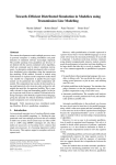
Figure 1. Simplified schematic of NVIDIA GPU
architecture, consisting of a set of Streaming
Multiprocessors (SM), each containing a number of Scalar
Processors (SP) with fast private memory and on-ship
local shared memory. The GPU also has off-chip DRAM.
The building block of the NVIDIA CUDA hardware
architecture is the Streaming Multiprocessor (SM). In
the NVIDIA Fermi-Tesla M2050 GPU, each SM contains 32 Scalar Processors (SPs). The entire GPU has
14 such SMs totaling to 448 SPs, as well as some offchip DRAM memory, see Figure 1. This gives a scalable architecture where the performance of the GPU can
be varied by having more or fewer SMs.
To be able to take advantage of this architecture a
program meant to run on the GPU, known as a kernel,
needs to be massively multi-threaded. A kernel is just a
C-function meant to execute on the GPU. When a kernel is executed on the GPU it is divided into thread
blocks, where each thread block contains an equal
number of threads. These thread blocks are automatically distributed among the SMs, so a programmer
need not consider the number of SMs a certain GPU
has. All threads execute one common instruction at a
time. If any threads take divergent execution paths,
then each of these paths will be executed separately,
and the threads will then converge again when all paths
have been executed. This means that some SPs will be
idle if the thread executions diverge. It is thus important that all threads agree on an execution path for
optimal performance.
This architecture is similar to the Single Instruction,
Multiple Data (SIMD) architecture that vector processors use, and that most modern general-purpose CPUs
have limited capabilities for too. NVIDIA call this architecture Single Instruction, Multiple Thread (SIMT)
instead, the difference being that each thread can execute independently, although at the cost of reduced performance. It is also possible to regard each SM as a
separate processor, which enables Multiple Instructions, Multiple Data (MIMD) parallelism. Using only
MIMD parallelism will not make it possible to take full
advantage of a GPU’s power, since each SM is a SIMD
processor. To summarize:
 Streaming Multiprocessors (SM) can work with different code, performing different operations with
entirely different data (MIMD execution, Multiple
Instruction Multiple Data).
 All Scalar processors (SP) in one streaming multiprocessor execute the same instruction at the same
time but work on different data (SIMT/SIMD execution, Single Instruction Multiple Data).
3.1.1
NVIDIA GPU Memory Hierarchy
As can be seen in Figure 1 there are several different
types of memory in the CUDA hardware architecture.
At the lowest level each SP has a set of registers, the
number depending on the GPU’s capabilities. These
registers are shared between all threads allocated to a
SM, so the number of thread blocks that a SM can have
active at the same time is limited by the register usage
of each thread. Accessing a register typically requires
no extra clock cycles per instruction, except for some
special cases where delays may occur.
Besides the registers there is also the shared (local)
memory, which is shared by all SPs in a SM. The
shared memory is implemented as fast on-chip
memory, and accessing the shared memory is generally
as fast as accessing a register. Since the shared memory
is accessible to all threads in a block it allows the
threads to cooperate efficiently by giving them fast access to the same data.
Most of the GPU memory is off-chip Dynamic
Random Access Memory (DRAM). The amount of off-
chip memory on modern graphics cards range from
several hundred megabytes to few gigabytes. The
DRAM memory is much slower than the on-chip memories, and is also the only memory that is accessible to
the host CPU, e.g. through DMA transfers. To summarize:
 Each scalar processor (SP) has a set of fast registers.
(private memory)
 Each streaming multiprocessor (SM) has a small local shared memory (48KB on Tesla M2050 ) with
relatively fast access.
 Each GPU device has a slower off-chip DRAM
(2GB on Tesla M2050) which is accessible from all
streaming multiprocessors and externally e.g. from
the CPU with DMA transfers.
3.2
OpenCL – the Open Computing Language
OpenCL [14] is the first open, free parallel computing
standard for cross-platform parallel programming of
modern processors including GPUs. The OpenCL programming language is based on C99 with some extensions for parallel execution management. By using
OpenCL it is possible to write parallel algorithms that
can be easily ported between multiple devices with
minimal or no changes to the source code.
The OpenCL framework consists of the OpenCL
programming language, API, libraries, and a runtime
system to support software development. The framework can be divided into a hierarchy of models: Platform Model, Memory model, Execution model, and
Programming model.
Figure 2. OpenCL platform architecture.
The OpenCL platform architecture in Figure 2 is similar to the NVIDIA CUDA architecture in Figure 1:





Compute device – Graphics Processing Unit (GPU)
Compute unit – Streaming Multiprocessor (SM)
Processing element – Scalar Processor (SP)
Work-item – thread
Work-group – thread block
The memory hierarchy (Figure 3) is also very similar:
 Global memory – GPU off-chip DRAM memory
 Constant memory – read-only cache of off-chip
memory
 Local memory – on-chip shared memory that can be
accessed by threads in the same SM
 Private memory – on-chip registers in the same
Figure 4. OpenCL execution model, work-groups
depicted as groups of squares corresponding to workitems. Each work-group can be referred to by a unique ID,
and each work-item by a unique local ID.
Figure 3. Memory hierarchy in the OpenCL memory
model, closely related to typical GPU architectures such
as NVIDIA.
The memory regions can be accessed in the following
way:
Memory Regions
Constant Memory
Local Memory
Private Memory
Global Memory
3.2.1
Access to Memory
All work-items in all work-groups
All work-items in a work-group
Private to a work-item
All work-items in all work-groups
OpenCL Execution Model
The execution of an OpenCL program consists of two
parts, the host program which executes on the host and
the parallel OpenCL program, i.e., a collection of kernels (also called kernel functions), which execute on
the OpenCL device. The host program manages the
execution of the OpenCL program.
Kernels are executed simultaneously by all threads
specified for the kernel execution. The number and
mapping of threads to Computing Units of the OpenCL
device is handled by the host program.
Each thread executing an instance of a kernel is
called a work-item. Each thread or work item has
unique id to help identify it. Work items can have additional id fields depending on the arrangement specified
by the host program.
Work-items can be arranged into work-groups. Each
work-group has a unique ID. Work-items are assigned
a unique local ID within a work-group so that a single
work-item can be uniquely identified by its global ID
or by a combination of its local ID and work-group ID.
The work-items in a given work-group execute concurrently on the processing elements of a single compute
unit as depicted in Figure 4.
Several programming models can be mapped onto
this execution model. OpenCL explicitly supports two
of these models: primarily the data parallel programming model, but also the task parallel programming
model
4
ParModelica: Extending Modelica
for Explicit Algorithmic Parallel
Programming
As mentioned in the introduction, the focus of the current work is an extension (ParModelica) of the algorithmic subset of Modelica for efficient explicit parallel
programming on highly data-parallel SPMD (Single
Program Multiple Data) architectures. The current
ParModelica implementation generates OpenCL [14]
code for parallel algorithms. OpenCL was selected instead of CUDA [15] because of its portability between
several multi-core platforms. Generating OpenCL code
ensures that simulations can be run with parallel support on OpenCL enabled Graphics and Central Processor Units (GPUs and CPUs). This includes many multicore CPUs from [19] and Advanced Micro Devices
(AMD) [18] as well as a range of GPUs from NVIDIA
[17] and AMD [18].
As mentioned earlier most previous work regarding
parallel execution support in the OpenModelica compiler has been focused on automatic parallelization
where the burden of finding and analyzing parallelism
has been put on the compiler. In this work, however,
we have decided to leave this responsibility to the end
user programmer. The compiler provides additional
high level language constructs needed for explicitly
stating parallelism in the algorithmic part of the modeling language. These, among others, include parallel
variables, parallel functions, kernel functions and paral-
lel for loops indicated by the parfor keyword. There are
also some target language specific constructs and functions (in this case related to OpenCL).
4.1
Parallel Variables
OpenCL code can be executed on a host CPU as well
as on GPUs whereas CUDA code executes only on
GPUs. Since the OpenCL and CUDA enabled GPUs
use their own local (different from CPU) memory for
execution, all necessary data should be copied to the
specific device's memory. Parallel variables are allocated on the specific device memory instead of the host
CPU. An example is shown below:
function parvar
protected
Integer m = 1000;
Integer A[m,m];
Integer B[m,m];
// global and local
parglobal Integer
parglobal Integer
parglobal Integer
parlocal Integer
parlocal Integer
end parvar;
// Host Scalar
// Host Matrix
// Host Matrix
device memories
pm;
// Global Scalar
pA[m,m];// Glob Matrix
pB[m,m];// Glob Matrix
pn;
// Local Scalar
pS[m]; // Local Array
The first two matrices A and B are allocated in normal
host memory. The next two matrices pA and pB are
allocated on the global memory space of the OpenCL
device to be used for execution. These global variables
can be initialized from normal or host variables. The
last array pS is allocated in the local memory space of
each processor on the OpenCL device. These variables
are shared between threads in a single work-group and
cannot be initialized from hast variables.
Copying of data between the host memory and the
device memory used for parallel execution is as simple
as assigning the variables to each other. The compiler
and the runtime system handle the details of the operation. The assignments below are all valid in the function given above
 Normal assignment - A := B
 Copy from host memory to parallel execution device memory - pA := A
 Copy from parallel execution device memory to
host memory - B := pB
 Copy from device memory to other device memory
– pA := pB
Modelica parallel arrays are passed to functions only by reference. This is done to reduce the rather expensive copy operations.
4.2
Parallel Functions
ParModelica parallel functions correspond to OpenCL
functions defined in kernel files or to CUDA device
functions. These are functions available for distributed
(parallel) independent execution in each thread executing on the parallel device. For example, if a parallel
array has been distributed with one element in each
thread, a parallel function may operate locally in parallel on each element. However, unlike kernel functions,
parallel functions cannot be called from serial code in
normal Modelica functions on the host computer just as
parallel OpenCL functions are not allowed to be called
from serial C code on the host. Parallel functions have
the following constraints, primarily since they are assumed to be called within a parallel context in workitems:
 Parallel function bodies may not contain parforloops. The reason is that the kernel containing the
parallel functions is already distributed on each
thread.
 Explicitly declared parallel variables are not allowed since execution is already taking place on the
parallel device.
 All memory allocation will be on the parallel device's memory.
 Nested parallelism as in NestStepModelica [10] is
not supported by this implementation.
 Called functions must be parallel functions or supported built-in functions since execution is on the
parallel device.
 Parallel functions can only be called from the body
of a parfor-loop, from parallel functions, or from
kernel functions.
Parallel functions in ParModelica are defined in the
same way as normal Modelica functions, except that
they are preceded by the parallel keyword as in the
multiply function below:
parallel function multiply
input parglobal Integer a;
input parlocal Integer b;
output parprivate Integer c;
output Integer c;
algorithm
c := a * b;
end multiply;
4.3
// same as
Kernel Functions
ParModelica kernel functions correspond to OpenCL
kernel functions [14] or CUDA global functions [16].
They are simply functions compiled to execute on an
OpenCL parallel device, typically a GPU. ParModelica
kernel functions are allowed to have several return- or
output variables unlike their OpenCL or CUDA counterparts. They can also allocate memory in the global
address space. Kernel functions can be called from serial host code, and are executed by each thread in the
launch of the kernel. Kernels functions share the first
three constraints stated above for parallel functions.
However, unlike parallel functions, kernel functions
cannot be called from the body of a parfor-loop or from
other kernel functions.
Kernel functions in ParModelica are defined in the
same way as normal Modelica functions, except that
they are preceded by the kernel keyword. An example
usage of kernel functions is shown by the kernel function arrayElemtWiseMult. The thread id function
oclGetGlobalId() (see Section 4.5) returns the integer
id of a work-item in the first dimension of a work
group.
kernel function arrayElemWiseMultiply
input Integer m;
input Integer A[m];
input Integer B[m];
output Integer C[m];
protected
Integer id;
algorithm
id := oclGetGlobalId(1);
// calling the parallel function
multiply is OK from kernel functions
C[id] := multiply(A[id],B[id]); //
multiply can be replaced by A[id]*B[id]
end arrayElemWiseMultiply;
4.4
ParModelica parallel for loops, compared to normal
Modelica for loops, have some additional constraints:
 All variable references in the loop body must be to
parallel variables.
 Iterations should not be dependent on other iterations i.e. no loop-carried dependencies.
 All function calls in the body should be to parallel
functions or supported built-in functions only.
4.5
// Matrix multiplication using parfor loop
parfor i in 1:m loop
for j in 1:pm loop
ptemp := 0;
for h in 1:pm loop // calling the
// parallel function multiply is OK
// from parfor-loops
ptemp := multiply(pA[i,h], pB[h,j])
+ ptemp;
end for;
pC[i,j] := ptemp;
end for;
end parfor;
OpenCL
Code
There are also some additional ParModelica features
available for directly compiling and executing userwritten OpenCL code:

oclbuild(String) takes a name of an OpenCL source
file and builds it. It returns an OpenCL program
object which can be used later.

oclkernel(oclprogram, String) takes a previously
built OpenCL program and create the kernel specified by the second argument. It returns an OpenCL
kernel object which can be used later.

oclsetargs(oclkernel,...) takes a previously created
kernel object variable and a variable number of arguments and sets each argument to its corresponding one in the kernel definition.

oclexecute(oclkernel) executes the specified kernel.
Parallel For Loop: parfor
The iterations of a ParModelica parfor-loop are executed without any specific order in parallel and independently by multiple threads. The iterations of a parfor-loop are equally distributed among available processing units. If the range of the iteration is smaller
than or equal to the number of threads the parallel device supports, each iteration will be done by a separate
thread. If the number of iterations is larger than the
number of threads available, some threads might perform more than one iteration. In future enhancements
parfor will be given the extra feature of specifying the
desired number of threads explicitly instead of automatically launching threads as described above. An
example of using the parfor-loop is shown below:
Executing User-written
from ParModelica.
All of the above operations are synchronous in the
OpenCL jargon. They will return only when the specified operation is completed. Further functionality is
planned to be added to these functions to provide better
control over execution.
4.6
Synchronization and Thread Management
All OpenCL work-item functions [20] are available in
ParModelica. They perform the same operations and
have the “same” types and number of arguments. However, there are two main differences:
 Thread/work-item index ids start from 1 in ParModelica, whereas the OpenCL C implementation
counts from 0.
 Array dimensions start from 1 in Modelica and
from 0 in OpenCL and C.
For example oclGetGlobalId(1) call in the above
arrayElemWiseMultiply will return the integer ID of
a work-item or thread in the first dimension of a work
group. The first thread gets an ID of 1. The OpenCL C
call
for
the
same
operation
would
be
ocl_get_global_id(0) with the first thread obtaining an ID of 0.
5
Benchmarking and Evaluation
To be able to evaluate the relative performance and
behavior of the new language extensions described in
Section 4, performing systematic benchmarking on a
set of appropriate Modelica models is required. For this
purpose we have constructed a benchmark test suite
containing some models that represent heavy and highperformance computation, relevant for simulation on
parallel architectures.
5.1
The MPAR Benchmark Suite
The MPAR benchmark test suite contains seven different algorithms from well-known benchmark applications such as the LINear equations software PACKage
(LINPACK) [21], and Heat Conduction [23]. These
benchmarks have been collected and implemented as
algorithmic time-independent Modelica models.
The algorithms implemented in this suite involve rather large computations and impose well defined workloads on the OpenModelica compiler and the run-time
system. Moreover, they include different kinds of forloops and function calls which provide parallelism for
domain and task decomposition. For space reasons we
have provided results for only three models here.
Time measurements have been performed of both
sequential and parallel implementations of three models: Matrix Multiplication, Eigen value computation,
and Stationary Heat Conduction, on both CPU and
GPU architectures. For executing sequential codes generated by the standard sequential OpenModelica compiler we have used the Intel Xeon E5520 CPU [24]
which has 16 cores, each with 2.27 GHz clock frequency. For executing generated code by our new OpenCL
based parallel code generator, we have used the same
CPU as well as the NVIDIA Fermi-Tesla M2050 GPU
[25].
5.2
Measurements
In this section we present the result of measurements
for simulating three models from the implemented
benchmark suite. On each hardware configuration all
simulations are performed five times with start time
0.0, stop time of 0.2 seconds and 0.2 seconds time step,
measuring the average simulation time using the
clock_gettime() function from the C standard li-
brary. This function is called once when the simulation
loop starts and once when the simulation loop finishes.
The difference between the returned values gives the
simulation time.
All benchmarks have been simulated on both the Intel Xeon E5520 CPU (16 cores) and the NVIDIA Fermi-Tesla M2050 GPU (448 cores).
5.3
Simulation Results
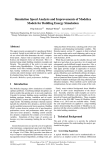
The Matrix Multiplication model (Appendix A) produces an M×K matrix C from multiplying an M×N matrix A by an N×K matrix B. This model presents a very
large level of data-parallelism for which a considerable
speedup has been achieved as a result of parallel simulation of this model on parallel platforms. The simulation results are illustrated in Figure 5 and Figure 6. The
obtained speedup of matrix multiplication using kernel
functions is as follows compared to the sequential algorithm on Intel Xeon E5520 CPU:
 Intel 16-core CPU – speedup 26
 NVIDIA 448-core GPU – speedup 115
Speedup
114,67
CPU E5520
GPU M2050
35,95
26,34
24,76
4,36 0,61
13,41
64
4,61
128
256
512
Parameter M (Matrix sizes MxM)
Figure 5. Speedup for matrix multiplication, Intel 16-core
CPU and Nvidia 448 core GPU.
The measured matrix multiplication model simulation
times can be found in Figure 6.
Simulation Time (second)
In addition to the above features, special built-in
functions for building user written OpenCL code directly from source code, creating a kernel, setting arguments to kernel and execution of kernels are also
available. In addition parallel versions of some built-in
algorithm functions are also available.
512
256
128
64
32
16
8
4
2
1
0,5
0,25
0,125
0,0625
32
64
128
256
512
CPU E5520 (Serial)
0,093
0,741
5,875
58,426
465,234
CPU E5520 (Parallel)
0,137
0,17
0,438
2,36
17,66
GPU M2050 (Parallel)
1,215
1,217
1,274
1,625
4,057
Figure 6. Simulation time for matrix multiplication, Intel
1-core, 16-core CPU, NVidia 448 core GPU.
The second benchmark model performs Eigen-value
computation, with the following speedups:
 Intel 16-core CPU – speedup 3
Simulation Time (second)
 NVIDIA 448-core GPU – speedup 48
Speedup
47,71
CPU E5520
GPU M2050
33,25
16,95
1,020,71
256
6,68
2,24
1,992,27
512
1024
2,75
2,51
2,32
2048
4096
Figure 7. Speedup for Eigen value computation as a
function of model array size, for Intel 16-core CPU and
NVIDIA 448 core GPU, compared to the sequential
algorithm on Intel Xeon E5520 CPU.
The measured simulation times for the Eigen-value
model are shown in Figure 8.
1024
512
Simulation Time (second)
128
256
512
1,543
5,116
16,7
52,462 147,411 363,114 574,057
CPU E5520 (Parallel) 3,049
5,034
8,385
23,413 63,419 144,747 208,789
GPU M2050 (Parallel) 7,188
7,176
7,373
7,853
CPU E5520 (Serial)
1024
2048
4096
8,695
8192
10,922 12,032
Figure 8. Simulation time for Eigen-value computation as
a function of model array size, for Intel 1-core CPU, 16core CPU, and NVIDIA 448 core GPU.
The third benchmark model computes stationary heat
conduction, with the following speedups:
 Intel 16-core CPU – speedup 7
 NVIDIA 448-core GPU – speedup 22
Speedup
22,46
CPU E5520
GPU M2050
10,1
2,04
5,85
4,21
0,22
128
0,87
256
6,23
6,41
3,32
512
1024
128
256
512
102
4
204
8
CPU E5520 (Serial)
1,958
7,903
32,104
122,754
487,342
CPU E5520 (Parallel)
0,959
1,875
5,488
19,711
76,077
GPU M2050 (Parallel)
8,704
9,048
9,67
12,153
21,694
8192
Figure 10. Simulation time (seconds) for heat conduction
model as a function of model size parameter M, for 1-core
CPU, 16-core CPU, and 448 core GPU.
Array size
256
128
64
32
16
8
4
2
1
512
256
128
64
32
16
8
4
2
1
0,5
2048
Parameter M (Matrix size MxM)
Figure 9. Speedup for the heat conduction model as a
function of model size parameter M, Intel 16-core CPU
and Nvidia 448 core GPU, compared to sequential
algorithm on Intel Xeon E5520 CPU.
The measured simulation times for the stationary heat
conduction model are shown in Figure 10.
According to the results of our measurements illustrated in Figure 5, Figure 7, and Figure 9, absolute
speedups of 114, 48, and 22 respectively were achieved
when running generated ParModelica OpenCL code on
the Fermi-Tesla M2050 GPU compared to serial code
on the Intel Xeon E5520 CPU with the largest data sizes.
It should be noted that when the problem size is not
very large the sequential execution has better performance than the parallel execution. This is not surprising since for executing even a simple code on OpenCL
devices it is required to create an OpenCL context within those devices, allocate OpenCL memory objects,
transfer input data from host to those memory objects,
perform computations, and finally transfer back the
result to the host. Consequently, performing all these
operations normally takes more time compared to the
sequential execution when the problem size is small.
It can also be seen that, as the sizes of the models
increase, the simulations get better relative performance
on the GPU compared to multi-core CPU. Thus, to fully utilize the power of parallelism using GPUs it is required to have large regular data structures which can
be operated on simultaneously by being decomposed to
all blocks and threads available on GPU. Otherwise,
executing parallel codes on a multi-core CPU would be
a better choice than a GPU to achieve more efficiency
and speedup.
6
Guidelines for Using the New Parallel Language Constructs
The most important task in all approaches regarding
parallel code generation is to provide an appropriate
way for analyzing and finding parallelism in sequential
codes. In automatic parallelization approaches, the
whole burden of this task is on the compiler and tool
developer. However, in explicit parallelization approaches as in this paper, it is the responsibility of the
modeler to analyze the source code and define which
parts of the code are more appropriate to be explicitly
parallelized. This requires a good understanding of the
concepts of parallelism to avoid inefficient and incorrect generated code. In addition, it is necessary to know
the constraints and limitations involved with using explicit parallel language constructs to avoid compile
time errors. Therefore we give some advice on how to
use the ParModelica language extensions to parallelize
Modelica models efficiently:
 Try to declare parallel variables as well as copy assignments among normal and parallel variables as
less as possible since the costs of data transfers from
host to devices and vice versa are very expensive.
 In order to minimize the number of parallel variables as well as data transfers between host and devices, it is better not to convert forloops with few iterations over simple operations to parallel for-loops
(parfor-loops).
 It is not always useful to have parallel variables and
parfor-loops in the body of a normal for-loop which
has many iterations. Especially in cases where there
are many copy assignments among normal and parallel variables.
 Although it is possible to declare parallel variables
and also parfor-loops in a function, there are no advantages when there are many calls to the function
(especially in the body of a big for-loop). This will
increase the number of memory allocations for parallel variables as well as the number of expensive
copies required to transfer data between host and
devices.
 Do not directly convert a for-loop to a parfor-loop
when the result of each iteration depends on other
iterations. In this case, although the compiler will
correctly generate parallel code for the loop, the result of the computation may be incorrect.
 Use a parfor-loop in situations where the loop has
many independent iterations and each iteration takes
a long time to be completed.
 Try to parallelize models using kernel functions as
much as possible rather than using parfor-loops.
This will enable you to explicitly specify the desired
number of threads and work-groups to get the best
performance.
 If the global work size (total number of threads to
be run in parallel) and the local work size (total
number of threads in each work-group) need to be
specified explicitly, then the following points
should be considered. First, the work-group size
(local size) should not be zero, and also it should
not exceed the maximum work-group size supported
by the parallel device. Second, the local size should
be less or equal than the global-size. Third, the
global size should be evenly divisible by the local
size.
 The current implementation of OpenCL does not
support recursive functions; therefore it is not possible to declare a recursive function as a parallel
function.
7
Conclusions
New multi-core CPU and GPU architectures promise
high computational power at a low cost if suitable
computational algorithms can be developed. The
OpenCL C-based parallel programming model provides
a way of writing portable parallel algorithms that perform well on a number of multi-core architectures.
However, the OpenCL programming model is rather
low-level and error-prone to use and intended for parallel programming specialists.
This paper presents the ParModelica algorithmic
language extension to the high-level Modelica modeling language together with a prototype implementation
in the OpenModelica compiler. This makes it possible
for the Modelica modeler to directly write efficient parallel algorithms in Modelica which are automatically
compiled to efficient low-level OpenCL code. A
benchmark suite called MPAR has been developed to
evaluate the prototype. Good speedups have been obtained for large problem sizes of matrix multiplication,
Eigen value computation, and stationary heat condition.
Future work includes integration of the ParModelica
explicit parallel programming approach with automatic
and semi-automatic approaches for compilation of
equation-based Modelica models to parallel code. Autotuning could be applied to further increase the performance and automatically adapt it to varying problem
configurations. Some of the ParModelica code needed
to specify kernel functions could be automatically generated.
8
Acknowledgements
This work has been supported by Serc, by Elliit, by the
Swedish Strategic Research Foundation in the EDOp
and HIPo projects and by Vinnova in the RTSIM and
ITEA2 OPENPROD projects. The Open Source Modelica Consortium supports the OpenModelica work.
Thanks to Per Östlund for contributions to Section 3.1.
References
[1] Modelica Association. The Modelica Language
Specification Version 3.2, March 24th 2010.
http://www.modelica.org. Modelica Association.
Modelica Standard Library 3.1. Aug. 2009.
http://www.modelica.org./
[2] Open Source Modelica Consortium. OpenModelica System Documentation Version 1.8.1, April
2012. http://www.openmodelica.org/
[3] Peter Fritzson. Principles of Object-Oriented
Modeling and Simulation with Modelica 2.1.
Wiley-IEEE Press, 2004.
[4] Peter Aronsson. Automatic Parallelization of
Equation-Based Simulation Programs, PhD thesis, Dissertation No. 1022, Linköping University,
2006.
[5] Håkan Lundvall. Automatic Parallelization using
Pipelining for Equation-Based Simulation Languages, Licentiate thesis No. 1381, Linköping
University, 2008.
[6] Håkan Lundvall, Kristian Stavåker, Peter
Fritzson, Christoph Kessler: Automatic Parallelization of Simulation Code for Equation-based
Models with Software Pipelining and Measurements on Three Platforms. MCC'08 Workshop,
Ronneby, Sweden, November 27-28, 2008.
[7] Per Östlund. Simulation of Modelica Models on
the CUDA Architecture. Master Thesis. LIUIDA/LITH-EX-A{09/062{SE. Linköping University, 2009.
[8] Kristian Stavåker, Peter Fritzson. Generation of
Simulation Code from Equation-Based Models
for Execution on CUDA-Enabled GPUs. MCC'10
Workshop, Gothenburg, Sweden, November 1819, 2010.
[9] Matthias Korch and Thomas Rauber. Scalable
parallel rk solvers for odes derived by the method
of lines. In Harald Kosch, Laszlo Böszörményi,
and Hermann Hellwagner, editors, Euro-Par, volume 2790 of Lecture Notes in Computer Science,
pages 830-839. Springer, 2003.
[10] Christoph Kessler and Peter Fritzson. NestStepModelica – Mathematical Modeling and BulkSynchronous Parallel Simulation. In Proc. of
PARA'06, Umeå, June 19-20, 2006. In Lecture
Notes of Computer Science (LNCS) Vol 4699, pp
1006-1015, Springer Verlag, 2006.
[11] Martin Sjölund, Robert Braun, Peter Fritzson and
Petter Krus. Towards Efficient Distributed Simulation in Modelica using Transmission Line Modeling. In Proceedings of the 3rd International
Workshop on Equation-Based Object-Oriented
Modeling Languages and Tools, (EOOLT'2010),
Published by Linköping University Electronic
Press, www.ep.liu.se, In conjunction with MODELS’2010, Oslo, Norway, Oct 3, 2010.
[12] Francois Cellier and Ernesto Kofman. Continuous
System Simulation. Springer, 2006.
[13] Khronos Group, Open Standards for Media Authoring and Acceleration, OpenCL 1.1, accessed
Sept 15, 2011. http://www.khronos.org/opencl/
[14] The OpenCL Specication, Version: 1.1, Document Revision: 44, accessed June 30 2011.
http://www.khronos.org/registry/cl/specs/opencl1.1.pdf
[15] NVIDIA CUDA, accessed September 15 2011.
http://www.nvidia.com/object/cuda
home
new.html
[16] NVIDIA CUDA programming guide, accessed 30
June 2011. http://developer.download.nvidia.com/
compute/cuda/4 0 rc2/toolkit/docs/CUDA C Programming Guide.pdf
[17] OpenCL Programming Guide for the CUDA Architecture, Appendix A, accessed June 30 2011.
http://developer.download.nvidia.com/compute/D
evZone/docs/html/OpenCL/doc/OpenCL
Programming Guide.pdf
[18] AMD OpenCL, System Requirements & Driver
Compatibility, accessed June 30 2011.
http://developer.amd.com/sdks/AMDAPPSDK/pa
ges/DriverCompatibility.aspx
[19] INTEL OpenCL, Technical Requirements, accessed
June
30
2011.
http://software.intel.com/enus/articles/openclrelease-notes/
[20] OpenCL Work-Item Built-In Functions, accessed
June
30
2011.
http://www.khronos.org/registry/cl/sdk/1.0/docs/
man/xhtml/workItemFunctions.html
[21] Jack J. Dongarra, J. Bunch, Cleve Moler, and G.
W. Stewart. LINPACK User's Guide. SIAM,
Philadelphia, PA, 1979.
[22] Ian N. Sneddon. Fourier Transforms. Dover Publications, 2010. ISBN-13: 978-0486685229.
[23] John H. Lienhard IV and John H. Lienhard V. A
Heat Transfer Textbook. Phlogiston Press Cambridge, Massachusetts, U.S.A, 4th edition, 2011.
[24] Intel Xeon E5520 CPU Specifications, accessed
October
28
2011.
http://ark.intel.com/products/40200/Intel-XeonProcessor-E5520-(8M-Cache-2 26-GHz-5 86GTs-Intel-QPI)
[25] NVIDIA Tesla M2050 GPU Specifications, accessed
June
30
2011.
http://www.nvidia.com/docs/IO/43395/BD05238-001 v03.pdf
[26] Cyril Faure. Real-time simulation of physical
models toward hardware-in-the-loop validation.
PhD Thesis. University of Paris East, October
2011.
Appendix A. Serial Matrix Multiply
model MatrixMultiplication
parameter Integer m=256 ,n=256 ,k =256;
Real result ;
algorithm
result := mainF (m,n,k);
end MatrixMultiplication ;
function mainF
input Integer m;
input Integer n;
input Integer k;
output Real result ;
protected
Real A[m,n];
Real B[n,k];
Real C[m,k];
algorithm
// initialize matrix A, and B
(A,B) := initialize (m,n,k);
// multiply matrices A and B
C := matrixMultiply (m,n,k,A,B);
// only one item is returned to speed up
// computation
result := C[m,k];
end mainF;
function initialize
input Integer m;
input Integer n;
input Integer k;
output Real A[m,n];
output Real B[n,k];
algorithm
for i in 1:m loop
for j in 1:n loop
A[i,j] := j;
end for;
end for;
for j in 1:n loop
for h in 1:k loop
B[j,h] := h;
end for;
end for;
end initialize ;
function matrixMultiply
input Integer m;
input Integer p;
input Integer n;
input Real A[m,p];
input Real B[p,n];
output Real C[m,n];
Real localtmp ;
algorithm
for i in 1:m loop
for j in 1:n loop
localtmp := 0;
for k in 1:p loop
localtmp := localtmp +(A[i,k]*
B[k,j]);
end for;
C[i,j] := localtmp ;
end for;
end for;
end matrixMultiply;
Appendix B. Parallel Matrix-Matrix
Multiplication with parfor and Kernel
functions
model MatrixMultiplicationP
parameter Integer m=32,n=32,k=32;
Real result;
algorithm
result := mainF(m,n,k);
end MatrixMultiplicationP ;
function mainF
input Integer m;
input Integer n;
input Integer k;
output Real result ;
protected
Real C[m,k];
parglobal Real pA[m,n];
parglobal Real pB[n,k];
parglobal Real pC[m,k];
parglobal Integer pm;
parglobal Integer pn;
parglobal Integer pk;
// the total number of global threads
// executing in parallel in the kernel
Integer globalSize [2] = {m,k};
// the total number of local threads
// in parallel in each workgroup
Integer localSize [2] = {16 ,16};
algorithm
// copy from host to device
pm := m;
pn := n;
pk := k;
(pA ,pB) := initialize(m,n,k,pn ,pk);
// specify the number of threads and
// workgroups
// to be used for a kernel function
// execution
oclSetNumThreads(globalSize, localSize);
pC := matrixMultiply(pn ,pA ,pB );
// copy matrix from device to host
// and resturn result
C := pC;
result := C[m,k];
// set the number of threads to
// the available number
// supported by device
oclSetNumThreads(0);
end mainF ;
function initialize
input Integer m;
input Integer n;
input Integer k;
input parglobal Integer pn;
input parglobal Integer pk;
output parglobal Real pA[m,n];
output parglobal Real pB[n,k];
algorithm
parfor i in 1:m loop
for j in 1: pn loop
pA[i,j] := j;
end for;
end parfor;
parfor j in 1:n loop
for h in 1: pk loop
pB[j,h] := h;
end for;
end parfor ;
end initialize ;
parkernel function matrixmultiply
input parglobal Integer pn;
input parglobal Real pA [: ,:];
input parglobal Real pB [: ,:];
output parglobal Real pC[size(pA,1),
size(pB,2)];
protected
Real plocaltmp ;
Integer i,j;
algorithm
// Returns unique global thread Id value
// for first and second dimension
i := oclGetGlobalId (1);
j := oclGetGlobalId (2);
plocaltmp := 0;
for h in 1: pn loop
plocaltmp := plocaltmp + (pA[i,h] *
pB[h,j]);
end for;
pC[i,j] := plocaltmp;
end matrixmultiply;
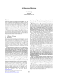
TLM and Parallelization
Martin Sjölund
December 3, 2012
Abstract
Transmission line modeling (TLM) is a technique where the wave propagation of a signal in a medium over time can be modelled. The propagation of this signal is limited by the time it takes for the signal to
travel across the medium. By utilizing this information it is possible to
partition the system of equations in such a way that the equations can
be partitioned into independent blocks that may be simulated in parallel. This leads to improved efficiency of simulations since it enables full
performance of multi-core CPUs.
1
Background and Related Work
An increasingly important way of creating efficient computations is to use parallel computing, i.e., dividing the computational work onto multiple processors
that are available in multi-core systems. Such systems may use either a CPU
[10] or a GPU using GPGPU techniques [13, 28]. Since multi-core processors are
becoming more common than single-core processors, it is becoming important
to utilize this resource. This requires support in compilers and development
tools.
However, while parallelization of models expressed in equation-based objectoriented (EOO) languages is not an easily solved task, the increased performance
if successful is important. A hardware-in-the-loop real-time simulator using
detailed computationally intensive models certainly needs the performance to
keep short real-time deadlines, as do large models that take days or weeks to
simulate. There are a few common approaches to parallelism in programming:
• No parallelism in the programming language, but accessible via library
calls. You can divide the work by executing several processes or jobs at
once, each utilizing one CPU core.
• Explicit parallelism in the language. You introduce language constructs
so that the programmer can express parallel computations using several
CPU cores.
• Automatic parallelization. The compiler itself analyzes the program or
model, partitions the work, and automatically produces parallel code.
1
Automatic parallelization is the preferred way because the users do not need
to learn how to do parallel programming, which is often error-prone and timeconsuming. This is even more true in the world of equation-based languages
because the ”programmer/modeler” can be a systems designer or modeler with
no real knowledge of programming or algorithms.
However, it is not so easy to do automatic parallelization of models in
equation-based languages. Not only is it needed to decide which processor to
perform a particular operation on; it is also needed to determine in which order
to schedule computations needed to solve the equation system.
This scheduling problem can become quite difficult and computationally expensive for large equation systems. It might also be hard to split the sequence of
operations into two separate threads due to dependencies between the equations
[1].
There are methods that can make automatic parallelization easier by introducing parallelism over time, e.g. distributing solver work over time [24].
However, parallelism over time gives very limited speedup for typical ODE systems of equations.
A single centralized solver is the normal approach to simulation in most
of today’s simulation tools. Although great advances have been made in the
development of algorithms and software, this approach suffers from inherent
poor scaling. That is, execution time grows more than linearly with system
size.
By contrast, distributed modeling, where solvers can be associated with
or embedded in subsystems, and even component models, has almost linear
scaling properties. Special considerations are needed, however, to connect the
subsystems to each other in a way that maintains stability properties without
introducing unwanted numerical effects. Technologies based on bilateral delay
lines [2], also called transmission line modeling, TLM, have been developed for
a long time at Linköping University. It has been successfully implemented in
the Hopsan simulation package, which is currently almost the only simulation
package that utilizes the technology, within mechanical engineering and fluid
power. It has also been demonstrated in [15] and subsequently in [4]. Although
the method has its roots already in the sixties, it has never been widely adopted,
probably because its advantages are not evident for small applications, and that
wave-propagation is regarded as a marginal phenomenon in most areas, and thus
not well understood.
In this paper we focus on introducing distributed simulation based on TLM
technology in Modelica, and combining this with solver inlining which further
contributes to avoiding the centralized solver bottleneck. In a future paper we
plan to demonstrate these techniques for parallel simulation.
Summarizing the main contents of the paper.
• We propose using a structured way of modeling with model partitioning using transmission lines in Modelica that is compatible with existing
Modelica tools (Section 6).
2
• We investigate two different methods to model transmission lines in Modelica and compare them to each other (Section 6).
• We show that such a system uses a distributed solver and may contain
subsystems with different time steps, which may improve simulation performance dramatically (Section 7).
• We demonstrate that solver inlining and distributed simulation using TLM
can be combined, and that the resulting simulation results are essentially
identical to those obtained using the Hopsan simulation package.
We use the Modelica language [7, 21] and the OpenModelica Compiler [8,
9] to implement our prototype, but the ideas should be valid for any similar
language.
1.1
Related Work
Several people have performed work on parallelization of Modelica models [1,
18, 19, 20, 23, 30], but there are still many unsolved problems to address.
The work closest to ours is [23], where Nyström uses transmission lines to
perform model partitioning for parallelization of Modelica simulations using
computer clusters. The problem with clusters is the communication overhead,
which is huge if communication is performed over a network. Real-time scheduling is also a bit hard to reason about if you connect your cluster nodes through
TCP/IP. Today, there is an increasing need to parallelize simulations on a single
computer because most CPUs are multi-core. One major benefit is communication costs; we will be able to use shared memory with virtually no delay in
interprocessor communication.
Another thing that is different between the two implementations is the way
TLM is modeled. We use regular Modelica models without function calls for
communication between model elements. Nyström used an external function
interface to do server-client communication. His method is a more explicit way
of parallelization, since he looks for the submodels that the user created and
creates a kind of co-simulation.
Inlining solvers have also been used in the past to introduce parallelism in
simulations [18].
Parallelization of Modelica-based simulation on GPUs has been explored by
Stavåker [27] and Östlund [30].
2
Transmission Line Element Method
A computer simulation model is basically a representation of a system of equations that model some physical phenomena. The goal of simulation software is
to solve this system of equations in an efficient, accurate and robust way. To
achieve this, the by far most common approach is to use a centralized solver
algorithm which puts all equations together into a differential algebraic equation
3
system (DAE) or an ordinary differential equation system (ODE). The system is
then solved using matrix operations and numeric integration methods. One disadvantage of this approach is that it often introduces data dependencies between
the central solver and the equation system, making it difficult to parallelize the
equations for simulation on multi-core platforms. Another problem is that the
stability of the numerical solver often will depend on the simulation time step.
An alternative approach is to let each component in the simulation model
solve its own equations, i.e. a distributed solver approach. This allows each
component to have its own fixed time step in its solvers. A special case where
this is especially suitable is the transmission line element method. Such a simulator has numerically highly robust properties, and a high potential for taking
advantage of multi-core platforms [14]. Despite these advantages, distributed
solvers have never been widely adopted and centralized solvers have remained
the de facto strategy on the simulation software market. One reason for this
can perhaps be the rapid increase in processor speed, which for many years
has made multi-core systems unnecessary and reduced the priority of increasing
simulation performance. Modeling for multi-core-based simulation also requires
applications of significant size for the advantages to become significant. With
the recent development towards an increase in the number of processor cores
rather than an increase in speed of each core, distributed solvers are likely to
play a more important role.
The fundamental idea behind the TLM method is to model a system in
a way such that components can be somewhat numerically isolated from each
other. This allows each component to solve its own equations independently
of the rest of the system. This is achieved by replacing capacitive components
(for example volumes in hydraulic systems) with transmission line elements of
a length for which the physical propagation time corresponds to one simulation
time step. In this way a time delay is introduced between the resistive components (for example orifices in hydraulic systems). The result is a physically
accurate description of wave propagation in the system [14]. The transmission
line element method (also called TLM method) originates from the method of
characteristics used in Hytran [16], and from Transmission Line Modeling [12],
both developed back in the nineteen sixties [2]. Today it is used in the Hopsan
simulation package for fluid power and mechanical systems, see Section 3, and
in the SKF TLM-based co-simulation package [25].
Mathematically, a transmission line can be described in the frequency domain by the four pole equation [29]. Assuming that friction can be neglected
and transforming these equations to the time domain, they can be described
according to equation 1 and 2.
p1 (t) = p2 (t − T ) + Zc q1 (t) + Zc q2 (t − T )
(1)
p2 (t) = p1 (t − T ) + Zc q2 (t) + Zc q1 (t − T )
(2)
Here p equals the pressure before and after the transmission line, q equals
the volume flow and Zc represents the characteristic impedance. The main
property of these equations is the time delay they introduce, representing the
4
x
Figure 1: Transmission line components calculate wave propagation through a
line using a physically correct separation in time.
communication delay between the ends of the transmission line, see Figure 1. In
order to solve these equations explicitly, two auxiliary variables are introduced,
see equations 3 and 4.
c1 (t) = p2 (t − T ) + Zc q2 (t − T )
(3)
c2 (t) = p1 (t − T ) + Zc q1 (t − T )
(4)
These variables are called wave variables or wave characteristics, and they represent the delayed communication between the end nodes. Putting equations
1 to 4 together will yield the final relationships between flow and pressure in
equations 5 and 6.
p1 (t) = c1 + Zc q1 (t)
(5)
p2 (t) = c2 + Zc q2 (t)
(6)
These equations can now be solved using boundary conditions. These are provided by adjacent (resistive) components. In the same way, the resistive components get their boundary conditions from the transmission line (capacitive)
components.
One noteworthy property with this method is that the time delay represents a physically correct separation in time between components of the model.
Since the wave propagation speed (speed of sound) in a certain liquid can be
calculated, the conclusion is that the physical length of the line is directly proportional to the time step used to simulate the component, see equation 7. Note
that this time step is a parameter in the component, and can very well differ
from the time step used by the simulation engine. Keeping the delay in the
5
transmission line larger than the simulation time step is important, to avoid
extrapolation of delayed values. This means that a minimum time delay of the
same size as the time step is required, introducing a modeling error for very
short transmission lines.
s
β
l = ha =
(7)
ρ
Here, h represents the time delay and a the wave propagation speed, while β
and ρ are the bulk modulus and the density of the liquid. With typical values
for the latter two, the wave propagation speed will be approximately 1000 m/s,
which means that a time delay of 1 ms will represent a length of 1 m. [15]
3
Hopsan
Hopsan is a simulation software for simulation and optimization of fluid power
and mechanical systems. This software was first developed at Linköping University in the late 1970’s [6]. The simulation engine is based on the transmission line
element method described in Section 2, with transmission lines (called C-type
components) and restrictive components (called Q-type) [17]. In the current
version, the solver algorithms are distributed so that each component uses its
own local solvers, although many common algorithms are placed in centralized
libraries.
In the new version of Hopsan, which is currently under development, all
equation solvers will be completely distributed as a result of an object-oriented
programming approach [3]. Numerical algorithms in Hopsan are always discrete. Derivatives are implemented by first or second order filters, i.e. a loworder rational polynomial expression as approximation, and using bilinear transforms, i.e. the trapetzoid rule, for numerical integration. Support for built-in
compatibility between Hopsan and Modelica is also being investigated.
4
Example Model with Pressure Relief Valve
The example model used for comparing TLM implementations in this paper is
a simple hydraulic system consisting of a volume with a pressure relief valve,
as can be seen in Figure 2. A pressure relief valve is a safety component, with
a spring at one end of the spool and the upstream pressure, i.e., the pressure
at the side of the component where the flow is into the component, acting on
the other end, see Figure 3. The preload of the spring will make sure that the
valve is closed until the upstream pressure reaches a certain level, when the force
from the pressure exceeds that of the spring. The valve then opens, reducing
the pressure to protect the system.
In this system the boundary conditions are given by a constant prescribed
flow source into the volume, and a constant pressure source at the other end of
the pressure relief valve representing the tank. As oil flows into the volume the
6
Figure 2: The example system consists of a volume and a pressure relief valve.
Boundary conditions is represented by a constant flow source and a constant
pressure source.
Figure 3: A pressure relief valve is designed to protect a hydraulic system by
opening at a specified maximum pressure.
pressure will increase at a constant rate until the reference pressure of the relief
valve is reached. The valve then opens, and after some oscillations a steady
state pressure level will appear.
A pressure relief valve is a very suitable example model when comparing
simulation tools. The reason for this is that it is based on dynamic equations
and also includes several non-linearities, making it an interesting component
to study. It also includes multiple physical domains, namely hydraulics and
mechanics. The opening of a relief valve can be represented as a step or ramp
response, which can be analyzed by frequency analysis techniques, for example using bode plots or Fourier transforms. It also includes several physical
phenomena useful for comparisons, such as wave propagations, damping and
self oscillations. If the complete set of equations is used, it will also produce
non-linear phenomena such as cavitation and hysteresis, although these are not
included in this paper.
The volume is modeled as a transmission line, in Hopsan known as a Ctype component. In practice this means that it will receive values for pressure
and flow from its neighboring components (flow source and pressure relief valve),
and return characteristic variables and impedance. The impedance is calculated
from bulk modulus, volume and time step, and is in turn used to calculate the
characteristic variables together with pressures and flows. There is also a low-
7
pass damping coefficient called α, which is set to zero and thereby not used in
this example.
mZc = mBulkmodulus/mVolume ∗ mTimestep ;
c10 = p2 + mZc ∗ q2 ;
c20 = p1 + mZc ∗ q1 ;
c1 = mAlpha∗ c1 + (1.0 −mAlpha ) ∗ c10 ;
c2 = mAlpha∗ c2 + (1.0 −mAlpha ) ∗ c20 ;
The pressure relief valve is a restrictive component, known as Q-type. This
means that it receives characteristic variables and impedance from its neighboring components, and returns flow and pressure. Advanced models of pressure
relief valves are normally performance oriented. This means that parameters
that users normally have little or no knowledge about, such as the inertia of the
spool or the stiffness of the spring are not needed as input parameters but are
instead implicitly included in the code. This is however complicated and not
very intuitive. For this reason a simpler model was created for this example. It
is basically a first-order force equilibrium equation with a mass, a spring and a
force from the pressure. Hysteresis and cavitation phenomena are also excluded
from the model.
The first three equations below calculate the total force acting on the spool.
By using a second-order filter, the x position can be received from Newton’s
second law. The position is used to retrieve the flow coefficient of the valve,
which in turn is used to calculate the flow using a turbulent flow algorithm.
Pressure can then be calculated from impedance and characteristic variables
according to transmission line modeling.
mFs = mPilotArea ∗ mPref ;
p1 = c1 + q1 ∗ Zc1 ;
Ftot = p1∗ mPilotArea − mFs ;
x0 = m F i l t e r . v a l u e ( Ftot ) ;
mTurb . s e t F l o w C o e f f i c i e n t (mCq∗mW∗ x0 ) ;
q2 = mTurb . getFlow ( c1 , c2 , Zc1 , Zc2 ) ;
q1 = −q2 ;
p1 = c1 + Zc1 ∗ q1 ;
p2 = c2 + Zc2 ∗ q2 ;
5
OpenModelica and Modelica
OpenModelica [8, 9] is an open-source Modelica-based modeling and simulation environment, whereas Modelica [21] is an equation-based, object-oriented
modeling/programming language. The Modelica Standard Library [22] contains
almost a thousand model components from many different application domains.
Modelica supports event handling as well as delayed expressions in equations.
We will use those properties later in our implementation of a distributed TLMstyle solver. It is worth mentioning that Hopsan may access the value of a state
8
variable, e.g. x, from the previous time step. This value may then be used to
calculate derivatives or do filtering since the length of time steps is fixed.
In standard Modelica, it is possible to access the previous value before an
event using the pre() operator, but impossible to access solver time-step related
values, since a Modelica model is independent of the choice of solver. This is
where sampling and delaying expressions comes into play. Note that while
delay(x,0) will return a delayed value, if the solver takes a time step > 0, it
will extrapolate information. Thus, it needs to take an infinite number of steps
to simulate the system, which means a delay time > 0 needs to be used.
6
Transmission Lines in an Equation-based Language
There are some issues when trying to use TLM in an equation-based language.
TLM has been proven to work well using fixed time steps. In Modelica
however, events can happen at any time. When an event is triggered due to
an event-inducing expression changing sign, the continuous-time solver is temporarily stopped and a root-finding solution process is started in order to find
the point in time where the event occurs. If the event occurs e.g. in the middle
of a fixed time step, the solver will need to take a smaller (e.g. half) time step
when restarted, i.e. some solvers may take extra time steps if the specified tolerance is not reached. However, this occurs only for hybrid models. For pure
continuous-time models which do not induce events, fixed steps will be kept
when using a fixed step solver.
The delay in the transmission line can be implemented in several ways. If
you have a system with fixed time steps, you get a sampled system. Sampling
works fine in Modelica, but requires an efficient Modelica tool since you typically
need to sample the system quite frequently. An example usage of the Modelica
sample() built-in function is shown below. Variables defined within whenequations in Modelica (as below) will have discrete-time variability.
when sample(−T, T) then
l e f t . c = p r e ( r i g h t . c ) + 2 ∗ Zc ∗ p r e ( r i g h t . q ) ;
r i g h t . c = p r e ( l e f t . c ) + 2 ∗ Zc ∗ p r e ( l e f t . q ) ;
end when ;
Modelica tools also offer the possibility to use delays instead of sampling. If
you use delays, you end up with continuous-time variables instead of discretetime ones. The methods are numerically very similar, but because the variables
are continuous when you use delay, the curve will look smoother.
l e f t . c = d e l a y ( r i g h t . c + 2 ∗ Zc ∗ r i g h t . q , T) ;
r i g h t . c = d e l a y ( l e f t . c + 2 ∗ Zc ∗ l e f t . q , T) ;
Finally, it is possible to explicitly specify a derivative rather than obtaining
it implicitly by difference computations relating to previous values (delays or
9
Figure 4: Pressure increases until the reference pressure of 10 MPa is reached,
where the relief valve opens.
Figure 5: Comparison of spool position using different TLM implementations.
sampling). This then becomes a transmission line without delay, which is a
good reference system.
d e r ( l e f t . p ) = ( l e f t . q+r i g h t . q ) /C ;
der ( r i g h t . p) = der ( l e f t . p) ;
Figure 4 contains the results of simulating our example system, i.e., the
pressure relief valve from section 4. Figures 5 and 6 are magnified versions that
show the difference between our different TLM implementations. The models
used to create the Figures, are part of the Modelica package DerBuiltin in
Appendix A.
If you decrease the delay in the transmission even closer to zero (it is now
10−4 ), the signals are basically the same (as would be expected). It does however come at a significant increase in simulation times and decreased numerical
stability. This is not acceptable if stable real-time performance is desired. We
use the same step size as the delay of the transmission line since that is the maximum allowed time step using this method, and better shows numerical issues
than a tiny step size.
Due to the nature of integrating solvers, we calculate the value der(x),
and use reinit() when der(x) changes sign. The OpenModelica dassl solver
cannot be used in all of these models due to an incompatibility with the delay()
operator (the solver does not limit its step size as it should). Dassl is used
together with sampling since the solver does limit its step size if a zero crossing
occurs; in the other simulations the Euler solver is used.
Because of these reasons we tried to use another method of solving the
equation system, see package DerInline in Appendix A. We simply inlined a
derivative approximation (x−delay(x,T))/T instead of der(x), which is much
closer to the discrete-time approximation used in the Hopsan model. This is
quite slow in practice because of the overhead delay adds, but it does implicitly
inline the solver, which is a good property for in parallelization.
If you look at Figures 7 and 8, you can see that all simulations now have
the same basic shape. In fact, the OpenModelica ones have almost the same
values. The time step is still 10−4 , which means you get the required behavior
even without sacrificing simulation times.
Even in this small example, the implementation using delays has 1 state
variable, while the ideal, zero-delay, implementation has 3 state variables. This
Figure 6: Comparison of system pressure using different TLM implementations.
10
Figure 7: Comparison of spool position with inlined explicit euler.
Figure 8: Comparison of system pressure with inlined explicit euler.
makes it easier to automatically parallelize larger models since the centralized
solver handles fewer calculations. When inlining the der() operator, we end up
with 0 continuous-time state variables.
Table 1 contains some performance numbers on the models used. At this
early stage in the investiagtion the numbers are not that informative for several
reasons.
We only made single-core simulations so far. Models that have better parallelism will get better speedups when we start doing multi-core simulations.
The current OpenModelica simulation runtime system implementation does
not have special efficient implementations of time events or delayed expressions.
The inlined solver uses delay explicitly instead of being an actual inlined
solver. This means it needs to search an array for the correct value rather than
accessing it directly, resulting in an overhead that will not exist once inline
solvers are fully implemented in OpenModelica.
We used the -noemit flag in OpenModelica to disable generation of result
files. Generating them takes between 20% and 90% of total simulation runtime
depending on solver and if many events are generated.
Do not compare the current Dymola [5] performance numbers to OpenModelica. We run Dymola inside a Windows virtual machine, while we run
OpenModelica on Linux.
The one thing that the performance numbers really tells you is not to use
sampling in OpenModelica until performance is improved, and that the overhead
of inlining the derivative using delay is a lot lower in Dymola than it is in
OpenModelica.
Table 1: Performance comparison between different models in the DerBuiltin
and DerInline packages.
Method
OpenModelica Delay
OpenModelica Ideal
OpenModelica Sample
Dymola Ideal
Dymola Sample
Builtin (sec)
0.13
0.04
3.65
0.64
1.06
11
Inlined (sec)
0.40
0.27
63.63
0.75
1.15
7
Distributed Solver
The implementation using an inlined solver in Section 6 is essentially a distributed solver. It may use different time steps in different submodels, which
means a system can be simulated using a very small time step only for certain
components. The advantage of such a distributed system becomes apparent in
[15].
In the current OpenModelica implementation this is not yet taken advantage
of, i.e., the states are solved in each time step regardless.
8
Further Work
To progress further we need to introduce replace the use of the delay() operator in the delay lines with an algorithm section. This would make the initial
equations easier to solve, the system would simulate faster, and it would retain
the property that connected subsystems don’t depend on each other.
Once we have partitioned a Modelica model into a distributed system model,
we will be able to start simulating the submodels in parallel, as described in
[11, 15].
Some of the problems inherent in parallelization of models expressed in EOO
languages are solved by doing this partitioning. By partitioning the model, you
essentially create many smaller systems, which are trivial to schedule on multicore systems.
To progress this work further a larger more computationally intensive model
is also needed. Once we have a good model and inlined solvers, we will work on
making sure that compilation and simulation scales well both with the target
number of processors and the size of the problem.
9
Conclusions
We conclude that all implementations work fine in Modelica.
The delay line implementation using delays is not considerably slower than
the one using the der() operator, but can be improved by using for example
algorithm sections here instead. Sampling also works fine, but is far too slow
for real-time applications. The delay implementation should be preferred over
using der(), since the delay will partition the whole system into subsystems,
which are easy to parallelize.
Approximating integration by inline euler using the delay operator is not
necessary to ensure stability although it produces results that are closer to the
results of the same simulation in Hopsan. When you view the simulation as a
whole, you can’t see any difference (Figure 4).
12

∗
∗



∗
∗
∗
∗




∗
∗



∗
∗
∗
∗
(a) Regular system



∗
∗
∗
∗
∗ ∗
∗
(c) Partitioned systems
(b) TLM system
Figure 9: Adjacency matrices in lower triangular form.
10
Partitioning
The reason for using TLM is that you implicitly gain a course-grained parallelization of the system. We present a general approach to partitioning a system
of equations that utilizes the time-delay introduced by TLM.
Each partition of the equation system will be independent from any other
within the current time step. This means they can be parallelized by synchronizing between time steps.
To illustrate what our algorithm does, consider the standard approach to
causalize (i.e. deciding what order and which assignments should be performed)
an equation system. The equation system is put in block lower triangle (BLT)
form, where each BLT block corresponds to either a single equation of the
original system or a strong component (several equations). The examples below
are lower triangular matrices (the strong components have been replaced with
a single one to make them easier to read). Since the matrix has no variables
above the diagonal (see Figure 9a), no block depends on a subsequent block and
the whole system can solved sequentially.
What happens when TLM is used to model the system is that some entries in
the adjacency matrix disappear since delay expressions are allowed to decouple
the system if they only access data in former time steps. In Figure 9b, one such
entry has been removed from Figure 9a. The new matrix can be cut into two
separate ones and solved sequentially in parallel since the two blocks are now
totally independent from each other (Figure 9c).
The basic data structure needed to perform this analysis is the incidence
matrix (which may be represented by an adjacency list or matrix depending on
the sparsity of the system). The benefit of only looking at the adjacency matrix
is that we may partition the equation system before we perform optimizations,
some of which are costly to perform on large systems since they do not have
linear time complexity.
10.1
Testcase
The testcase (see Appendix A) is a scalable version of the model in [26], where
instead of a volume, we can scale it to a sequence of volumes and orifices.
This means the automatic partitioning will be able to create a lot of independent subsystems, which can then be run in parallel (synchronized only between
13
timesteps).
10.2
Algorithm
...
11
Restrictions
Step size of the solver has to be enforced to be lower than or equal to the delay
of the shortest delay line in the system.
12
Runtime
The runtime uses OpenMP to run the independent equation systems in parallel.
The main changes to the runtime is that it needs to be thread-safe.
References
[1] Peter Aronsson. Automatic Parallelization of Equation-Based Simulation
Programs. Doctoral thesis No 1022, Linköping University, Department of
Computer and Information Science, June 2006.
[2] D. M. Auslander. Distributed System Simulation with Bilateral Delay-Line
Models. Journal of Basic Engineering, Trans. ASME:195–200, 1968.
[3] Mikael Axin, Robert Braun, Petter Krus, Alessandro dell’Amico, Björn
Eriksson, Peter Nordin, Karl Pettersson, and Ingo Staack. Next Generation
Simulation Software using Transmission Line Elements. In Proceedings of
the Bath/ASME Symposium on Fluid Power and Motion Control (FPMC),
Sep 2010.
[4] JD Burton, KA Edge, and CR Burrows. Partitioned Simulation of Hydraulic Systems Using Transmission-Line Modelling. In ASME WAM, 1993.
[5] Dassault Systèmes. Dymola 7.3, 2009.
[6] Björn Eriksson, Peter Nordin, and Petter Krus. Hopsan, A C++ Implementation Utilising TLM Simulation Technique. In Proceedings of the 51st
Conference on Simulation and Modelling (SIMS), October 2010.
[7] Peter Fritzson. Principles of Object-Oriented Modeling and Simulation with
Modelica 2.1. Wiley-IEEE Press, February 2004.
[8] Peter Fritzson, Peter Aronsson, Håkan Lundvall, Kaj Nyström, Adrian
Pop, Levon Saldamli, and David Broman. The OpenModelica Modeling,
Simulation, and Software Development Environment. Simulation News Europe, 44/45, December 2005.
14
[9] Peter Fritzson et al. Openmodelica 1.5.0 system documentation, June 2010.
[10] Jason Howard et al. A 48-core IA-32 message-passing processor with DVFS
in 45nm CMOS. In Solid-State Circuits Conference Digest of Technical
Papers (ISSCC), 2010 IEEE International, pages 108 –109, 7-11 2010.
[11] Arne Jansson, Petter Krus, and Jan-Ove Palmberg. Real Time Simulation
Using Parallel Processing. In The 2nd Tampere International Conference
on Fluid Power, 1991.
[12] P. B. Johns and M. A. O’Brien. Use of the transmission line modelling
(t.l.m) method to solve nonlinear lumped networks. The Radio and Electronic Engineer, 50(1/2):59–70, 1980.
[13] David B. Kirk and Wen-Mei W. Hwu. Programming Massively Parallel
Processors: A Hands-On Approach. Morgan Kaufmann Publishers, 2010.
[14] Petter Krus. Robust System Modelling Using Bi-lateral Delay Lines. In
Proceedings of the 2nd Conference on Modeling and Simulation for Safety
and Security (SimSafe), Linköping, Sweden, 2005.
[15] Petter Krus, Arne Jansson, Jan-Ove Palmberg, and Kenneth Weddfelt.
Distributed Simulation of Hydromechanical Systems. In The Third Bath
International Fluid Power Workshop, 1990.
[16] Air Force Aero Propulsion Laboratory. Aircraft hydraulic system dynamic
analysis. Technical report, Air Force Aero Propulsion Laboratory, AFAPLTR-76-43, Ohio, USA, 1977.
[17] Linköping University, Linköping University. The hopsan Simulation Program, User’s Manual, 1985. LiTH-IKP-R-387.
[18] Håkan Lundvall. Automatic Parallelization using Pipelining for EquationBased Simulation Languages. Licentiate thesis No 1381, Linköping University, Department of Computer and Information Science, 2008.
[19] Håkan Lundvall, Kristian Stavåker, Peter Fritzson, and Christoph Kessler.
Automatic Parallelization of Simulation Code for Equation-based Models
with Software Pipelining and Measurements on Three Platforms. Computer
Architecture News. Special Issue MCC08 – Multi-Core Computing, 36(5),
December 2008.
[20] Martina Maggio, Kristian Stavåker, Filippo Donida, Francesco Casella,
and Peter Fritzson. Parallel Simulation of Equation-based Object-Oriented
Models with Quantized State Systems on a GPU. In Proceedings of the 7th
International Modelica Conference, September 2009.
[21] Modelica Association. Modelica: A unified object-oriented language for
physical systems modeling, language specification version 3.2, 2010.
15
[22] Modelica Association. Modelica Standard Library version 3.1, 2010.
[23] Kaj Nyström and Peter Fritzson. Parallel Simulation with Transmission
Lines in Modelica. In Christian Kral and Anton Haumer, editors, Proceedings of the 5th International Modelica Conference, volume 1, pages 325–331.
Modelica Association, September 2006.
[24] Thomas Rauber and Gudula Rünger. Parallel execution of embedded and
iterated runge-kutta methods. Concurrency - Practice and Experience,
11(7):367–385, 1999.
[25] Alexander Siemers, Dag Fritzson, and Peter Fritzson. Meta-Modeling for
Multi-Physics Co-Simulations applied for OpenModelica. In Proceedings
of International Congress on Methodologies for Emerging Technologies in
Automation (ANIPLA), November 2006.
[26] Martin Sjölund, Robert Braun, Peter Fritzson, and Petter Krus. Towards
efficient distributed simulation in Modelica using transmission line modeling. In Peter Fritzon, Edward Lee, François Cellier, and David Broman,
editors, Proceedings of the 3rd International Workshop on Equation-Based
Object-Oriented Modeling Languages and Tools, pages 71–80. Linköping
University Electronic Press, October 2010.
[27] Kristian Stavåker. Contributions to Parallel Simulation of Equation-Based
Models on Graphics Processing Units. Licentiate thesis No 1507, Linköping
University, Department of Computer and Information Science, 2011.
[28] Ryoji Tsuchiyama, Takashi Nakamura, Takuro Iizuka, Akihiro Asahara,
and Satoshi Miki. The OpenCL Programming Book. Fixstars Corporation,
2010.
[29] T. J. Viersma. Analysis, Synthesis and Design of Hydraulic Servosystems
and Pipelines. Elsevier Scientific Publishing Company, Amsterdam, The
Netherlands, 1980.
[30] Per Östlund. Simulation of Modelica Models on the CUDA Architecture.
Master’s thesis, Linköping University, Department of Computer and Information Science, November 2009.
A
ParallelPRV
package TLM
connector Connector Q
output Real p ;
output Real q ;
input Real c ;
16
input Real Zc ;
end Connector Q ;
connector Connector C
input Real p ;
input Real q ;
output Real c ;
output Real Zc ;
end Connector C ;
model FlowSource
Connector Q s o u r c e ;
parameter Real f l o w V a l ;
equation
so ur ce .q = flowVal ;
source.p = source.c + source.q ∗ source.Zc ;
end FlowSource ;
model P r e s s u r e S o u r c e
Connector C p r e s s u r e ;
parameter Real P ;
equation
pressure.c = P;
pressure.Zc = 0;
end P r e s s u r e S o u r c e ;
model H y d r a u l i c A l t e r na t i v e P R V
Connector Q l e f t ;
Connector Q r i g h t ;
parameter Real P r e f = 20000000 ” R e f e r e n c e Opening
Pressure ” ;
parameter Real cq = 0 . 6 7 ” Flow C o e f f i c i e n t ” ;
parameter Real s p o o l d i a m e t e r = 0 . 0 1 ” S p o o l Diameter ” ;
parameter Real f r a c = 1 . 0 ” F r a c t i o n o f S p o o l
C i r c u m f e r e n c e t h a t i s Opening ” ;
parameter Real W = s p o o l d i a m e t e r ∗ f r a c ;
parameter Real p i l o t a r e a = 0 . 0 0 1 ” Working Area o f P i l o t
Pressure ” ;
parameter Real k = 1 e6 ” S t e a d y S t a t e C h a r a c t e r i s t i c s o f
Spring ” ;
parameter Real c = 1000 ” S t e a d y S t a t e Damping
Coefficient” ;
parameter Real m = 0 . 0 1 ”Mass” ;
parameter Real x h y s t = 0 . 0 ” H y s t e r e s i s o f S p o o l
Position ” ;
17
constant Real xmax = 0 . 0 0 1 ”Maximum S p o o l P o s i t i o n ” ;
constant Real xmin = 0 ”Minimum S p o o l P o s i t i o n ” ;
parameter Real T ;
parameter Real Fs = p i l o t a r e a ∗ P r e f ;
Real Ftot = l e f t . p ∗ p i l o t a r e a − Fs ;
Real Ks = cq ∗W∗x ;
Real x ( s t a r t = xmin, min = xmin, max = xmax ) ;
parameter I n t e g e r one = 1 ;
Real x f r a c = x∗ P r e f /xmax ;
Real v = der ( xtmp ) ;
Real a = der ( v ) ;
Real v2 = c ∗v ;
Real x2 = k∗x ;
Real xtmp ;
equation
left.p = left.c + left.Zc∗ left.q ;
right.p = right.c + right.Zc ∗ right.q ;
l e f t . q = −r i g h t . q ;
r i g h t . q = s i g n ( l e f t . c − r i g h t . c ) ∗ Ks ∗ ( noEvent ( s q r t ( abs
( l e f t . c − r i g h t . c ) +(( l e f t . Z c+r i g h t . Z c ) ∗Ks ) ˆ 2 / 4 ) ) − Ks
∗ ( l e f t . Z c+r i g h t . Z c ) / 2 ) ;
xtmp = ( Ftot − c ∗v − m∗ a ) /k ;
x = i f noEvent ( xtmp < xmin ) then xmin e l s e i f noEvent (
xtmp > xmax ) then xmax e l s e xtmp ;
end H y d r a u l i c A l t e r n a t i v e P R V ;
model Volume
parameter Real V;
parameter Real Be ;
f i n a l parameter Real Zc = Be∗T/V;
parameter Real T ;
Connector C l e f t ;
Connector C r i g h t ;
equation
l e f t . Z c = Zc ;
r i g h t . Z c = Zc ;
l e f t . c = d e l a y ( r i g h t . c +2∗Zc∗ r i g h t . q , T ) ;
r i g h t . c = d e l a y ( l e f t . c +2∗Zc∗ l e f t . q , T ) ;
end Volume ;
18
model O r i f i c e
parameter Real K;
Connector Q l e f t ;
Connector Q r i g h t ;
equation
l e f t . q = ( r i g h t . p − l e f t . p ) ∗K;
r i g h t . q = −l e f t . q ;
left.p = left.c + left.Zc∗ left.q ;
right.p = right.c + right.Zc ∗ right.q ;
end O r i f i c e ;
end TLM;
model PRVSystem
import TLM.{
Volume,Orifice,FlowSource,PressureSource,HydraulicAlternativePRV
};
constant Boolean b = f a l s e ;
parameter Real T = 1e−4 ;
Volume volume1 ( f i n a l V=1 e − 3 , f i n a l Be=1 e 9 , f i n a l T=T) ;
O r i f i c e o r i f i c e 1 ( f i n a l K=1) i f b ;
Volume volume2 ( f i n a l V=1 e − 3 , f i n a l Be=1 e 9 , f i n a l T=T) i f
b;
FlowSource f l o w S o u r c e ( f l o w V a l = 1e−5 ) ;
P r e s s u r e S o u r c e p r e s s u r e S o u r c e (P = 1 e5 ) ;
H y d r a u l i c A l t e r n a t i v e P R V hydr ( P r e f=1 e 7 , c q = 0 . 6 7 ,
s p o o l d i a m e t e r = 0 . 0 0 2 5 , f r a c = 1 . 0 , p i l o t a r e a =5e−5,xmax
= 0 . 0 1 5 ,m= 0 . 1 2 , c =400, k =150000,T=T) ;
equation
connect ( f l o w S o u r c e . s o u r c e , v o l u m e 1 . l e f t ) ;
i f b then
connect ( v o l u m e 1 . r i g h t , o r i f i c e 1 . l e f t ) ;
connect ( o r i f i c e 1 . r i g h t , v o l u m e 2 . l e f t ) ;
connect ( v o l u m e 2 . r i g h t , h y d r . l e f t ) ;
else
connect ( v o l u m e 1 . r i g h t , h y d r . l e f t ) ;
end i f ;
connect ( h y d r . r i g h t , p r e s s u r e S o u r c e . p r e s s u r e ) ;
end PRVSystem ;
19