Download Fulltext - LiU E-Press

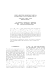
Towards Efficient Distributed Simulation in Modelica using
Transmission Line Modeling
Martin Sjölund1
1
Robert Braun2
Petter Krus2
Dept. of Computer and Information Science, Linköping University, Sweden,
{martin.sjolund,peter.fritzson}@liu.se
2
Dept. of Management and Engineering, Linköping University, Sweden,
{robert.braun,petter.krus}@liu.se
Abstract
The current development towards multiple processor cores
in personal computers is making distribution and parallelization of simulation software increasingly important.
The possible speedups from parallelism are however often limited with the current centralized solver algorithms,
which are commonly used in today’s simulation environments. An alternative method investigated in this work utilizes distributed solver algorithms using the transmission
line modeling (TLM) method. Creation of models using
TLM elements to separate model components makes them
very suitable for computation in parallel because larger
models can be partitioned into smaller independent submodels. The computation time can also be decreased by using small numerical solver step sizes only on those few submodels that need this for numerical stability. This is especially relevant for large and demanding models. In this paper we present work in how to combine TLM and solver inlining techniques in the Modelica equation-based language,
giving the potential for efficient distributed simulation of
model components over several processors.
Keywords TLM, transmission lines, distributed modeling, Modelica, H OPSAN, parallelism, compilation
1.
Peter Fritzson1
Introduction
An increasingly important way of creating efficient computations is to use parallel computing, i.e., dividing the computational work onto multiple processors that are available
in multi-core systems. Such systems may use either a CPU
[11] or a GPU using GPGPU techniques [14, 26]. Since
multi-core processors are becoming more common than
single-core processors, it is becoming important to utilize
this resource. This requires support in compilers and development tools.
3rd International Workshop on Equation-Based Object-Oriented
Languages and Tools. October, 2010, Oslo, Norway.
Copyright is held by the author/owner(s). The proceedings are published by
Linköping University Electronic Press. Proceedings available at:
http://www.ep.liu.se/ecp/047/
EOOLT 2010 website:
http://www.eoolt.org/2010/
However, while parallelization of models expressed in
equation-based object-oriented (EOO) languages is not an
easily solved task, the increased performance if successful
is important. A hardware-in-the-loop real-time simulator
using detailed computationally intensive models certainly
needs the performance to keep short real-time deadlines, as
do large models that take days or weeks to simulate. There
are a few common approaches to parallelism in programming:
• No parallelism in the programming language, but acces-
sible via library calls. You can divide the work by executing several processes or jobs at once, each utilizing
one CPU core.
• Explicit parallelism in the language. You introduce lan-
guage constructs so that the programmer can express
parallel computations using several CPU cores.
• Automatic parallelization. The compiler itself analyzes
the program or model, partitions the work, and automatically produces parallel code.
Automatic parallelization is the preferred way because
the users do not need to learn how to do parallel programming, which is often error-prone and time-consuming. This
is even more true in the world of equation-based languages
because the "programmer/modeler" can be a systems designer or modeler with no real knowledge of programming
or algorithms.
However, it is not so easy to do automatic parallelization of models in equation-based languages. Not only is it
needed to decide which processor to perform a particular
operation on; it is also needed to determine in which order to schedule computations needed to solve the equation
system.
This scheduling problem can become quite difficult and
computationally expensive for large equation systems. It
might also be hard to split the sequence of operations
into two separate threads due to dependencies between the
equations [2].
There are methods that can make automatic parallelization easier by introducing parallelism over time, e.g. distributing solver work over time [24]. However, parallelism
71
over time gives very limited speedup for typical ODE systems of equations.
A single centralized solver is the normal approach to
simulation in most of today’s simulation tools. Although
great advances have been made in the development of algorithms and software, this approach suffers from inherent
poor scaling. That is, execution time grows more than linearly with system size.
By contrast, distributed modeling, where solvers can be
associated with or embedded in subsystems, and even component models, has almost linear scaling properties. Special considerations are needed, however, to connect the
subsystems to each other in a way that maintains stability properties without introducing unwanted numerical effects. Technologies based on bilateral delay lines [3], also
called transmission line modeling, TLM, have been developed for a long time at Linköping University. It has been
successfully implemented in the H OPSAN simulation package, which is currently almost the only simulation package
that utilizes the technology, within mechanical engineering and fluid power. It has also been demonstrated in [16]
and subsequently in [5]. Although the method has its roots
already in the sixties, it has never been widely adopted,
probably because its advantages are not evident for small
applications, and that wave-propagation is regarded as a
marginal phenomenon in most areas, and thus not well understood.
In this paper we focus on introducing distributed simulation based on TLM technology in Modelica, and combining this with solver inlining which further contributes to
avoiding the centralized solver bottleneck. In a future paper
we plan to demonstrate these techniques for parallel simulation.
Summarizing the main contents of the paper.
• We propose using a structured way of modeling with
model partitioning using transmission lines in Modelica
that is compatible with existing Modelica tools (Section
6).
• We investigate two different methods to model trans-
mission lines in Modelica and compare them to each
other (Section 6).
• We show that such a system uses a distributed solver
and may contain subsystems with different time steps,
which may improve simulation performance dramatically (Section 7).
• We demonstrate that solver inlining and distributed sim-
ulation using TLM can be combined, and that the resulting simulation results are essentially identical to those
obtained using the H OPSAN simulation package.
We use the Modelica language [8, 21] and the OpenModelica Compiler [9, 10] to implement our prototype, but
the ideas should be valid for any similar language.
2.
Transmission Line Element Method
ena. The goal of simulation software is to solve this system
of equations in an efficient, accurate and robust way. To
achieve this, the by far most common approach is to use
a centralized solver algorithm which puts all equations together into a differential algebraic equation system (DAE)
or an ordinary differential equation system (ODE). The system is then solved using matrix operations and numeric
integration methods. One disadvantage of this approach is
that it often introduces data dependencies between the central solver and the equation system, making it difficult to
parallelize the equations for simulation on multi-core platforms. Another problem is that the stability of the numerical solver often will depend on the simulation time step.
An alternative approach is to let each component in the
simulation model solve its own equations, i.e. a distributed
solver approach. This allows each component to have its
own fixed time step in its solvers. A special case where
this is especially suitable is the transmission line element
method. Such a simulator has numerically highly robust
properties, and a high potential for taking advantage of
multi-core platforms [15]. Despite these advantages, distributed solvers have never been widely adopted and centralized solvers have remained the de facto strategy on the
simulation software market. One reason for this can perhaps be the rapid increase in processor speed, which for
many years has made multi-core systems unnecessary and
reduced the priority of increasing simulation performance.
Modeling for multi-core-based simulation also requires applications of significant size for the advantages to become
significant. With the recent development towards an increase in the number of processor cores rather than an increase in speed of each core, distributed solvers are likely
to play a more important role.
The fundamental idea behind the TLM method is to
model a system in a way such that components can be
somewhat numerically isolated from each other. This allows each component to solve its own equations independently of the rest of the system. This is achieved by replacing capacitive components (for example volumes in
hydraulic systems) with transmission line elements of a
length for which the physical propagation time corresponds
to one simulation time step. In this way a time delay is
introduced between the resistive components (for example
orifices in hydraulic systems). The result is a physically accurate description of wave propagation in the system [15].
The transmission line element method (also called TLM
method) originates from the method of characteristics used
in H YTRAN [17], and from Transmission Line Modeling
[13], both developed back in the nineteen sixties [3]. Today it is used in the H OPSAN simulation package for fluid
power and mechanical systems, see Section 3, and in the
SKF TLM-based co-simulation package [25].
Mathematically, a transmission line can be described
in the frequency domain by the four pole equation [27].
Assuming that friction can be neglected and transforming
these equations to the time domain, they can be described
according to equation 1 and 2.
A computer simulation model is basically a representation
of a system of equations that model some physical phenom-
p1 (t) = p2 (t − T ) + Zc q1 (t) + Zc q2 (t − T )
72
(1)
p1,q1
Zc
3.
p2,q2
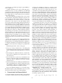
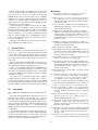
Figure 1. Transmission line components calculate wave
propagation through a line using a physically correct separation in time.
p2 (t) = p1 (t − T ) + Zc q2 (t) + Zc q1 (t − T )
(2)
Here p equals the pressure before and after the transmission
line, q equals the volume flow and Zc represents the characteristic impedance. The main property of these equations
is the time delay they introduce, representing the communication delay between the ends of the transmission line, see
Figure 1. In order to solve these equations explicitly, two
auxiliary variables are introduced, see equations 3 and 4.
c1 (t) = p2 (t − T ) + Zc q2 (t − T )
(3)
c2 (t) = p1 (t − T ) + Zc q1 (t − T )
(4)
These variables are called wave variables or wave characteristics, and they represent the delayed communication between the end nodes. Putting equations 1 to 4 together will
yield the final relationships between flow and pressure in
equations 5 and 6.
p1 (t) = c1 + Zc q1 (t)
(5)
p2 (t) = c2 + Zc q2 (t)
(6)
These equations can now be solved using boundary conditions. These are provided by adjacent (resistive) components. In the same way, the resistive components get their
boundary conditions from the transmission line (capacitive) components.
One noteworthy property with this method is that the
time delay represents a physically correct separation in
time between components of the model. Since the wave
propagation speed (speed of sound) in a certain liquid can
be calculated, the conclusion is that the physical length of
the line is directly proportional to the time step used to
simulate the component, see equation 7. Note that this time
step is a parameter in the component, and can very well
differ from the time step used by the simulation engine.
Keeping the delay in the transmission line larger than the
simulation time step is important, to avoid extrapolation of
delayed values. This means that a minimum time delay of
the same size as the time step is required, introducing a
modeling error for very short transmission lines.
s
β
(7)
l = ha =
ρ
Here, h represents the time delay and a the wave propagation speed, while β and ρ are the bulk modulus and the density of the liquid. With typical values for the latter two, the
wave propagation speed will be approximately 1000 m/s,
which means that a time delay of 1 ms will represent a
length of 1 m. [16]
H OPSAN
H OPSAN is a simulation software for simulation and optimization of fluid power and mechanical systems. This software was first developed at Linköping University in the late
1970’s [7]. The simulation engine is based on the transmission line element method described in Section 2, with
transmission lines (called C-type components) and restrictive components (called Q-type) [1]. In the current version,
the solver algorithms are distributed so that each component uses its own local solvers, although many common
algorithms are placed in centralized libraries.
In the new version of H OPSAN, which is currently under
development, all equation solvers will be completely distributed as a result of an object-oriented programming approach [4]. Numerical algorithms in H OPSAN are always
discrete. Derivatives are implemented by first or second
order filters, i.e. a low-order rational polynomial expression as approximation, and using bilinear transforms, i.e.
the trapetzoid rule, for numerical integration. Support for
built-in compatibility between H OPSAN and Modelica is
also being investigated.
4.
Example Model with Pressure Relief
Valve
The example model used for comparing TLM implementations in this paper is a simple hydraulic system consisting
of a volume with a pressure relief valve, as can be seen
in Figure 2. A pressure relief valve is a safety component,
with a spring at one end of the spool and the upstream pressure, i.e., the pressure at the side of the component where
the flow is into the component, acting on the other end, see
Figure 3. The preload of the spring will make sure that the
valve is closed until the upstream pressure reaches a certain level, when the force from the pressure exceeds that of
the spring. The valve then opens, reducing the pressure to
protect the system.
In this system the boundary conditions are given by
a constant prescribed flow source into the volume, and a
constant pressure source at the other end of the pressure
relief valve representing the tank. As oil flows into the
volume the pressure will increase at a constant rate until
the reference pressure of the relief valve is reached. The
valve then opens, and after some oscillations a steady state
pressure level will appear.
A pressure relief valve is a very suitable example model
when comparing simulation tools. The reason for this is
that it is based on dynamic equations and also includes
several non-linearities, making it an interesting component
to study. It also includes multiple physical domains, namely
hydraulics and mechanics. The opening of a relief valve
can be represented as a step or ramp response, which can
be analyzed by frequency analysis techniques, for example
using bode plots or Fourier transforms. It also includes
several physical phenomena useful for comparisons, such
as wave propagations, damping and self oscillations. If
the complete set of equations is used, it will also produce
non-linear phenomena such as cavitation and hysteresis,
although these are not included in this paper.
73
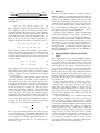
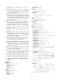
Figure 2. The example system consists of a volume and
a pressure relief valve. Boundary conditions is represented
by a constant flow source and a constant pressure source.
Figure 3. A pressure relief valve is designed to protect
a hydraulic system by opening at a specified maximum
pressure.
The volume is modeled as a transmission line, in H OP known as a C-type component. In practice this means
that it will receive values for pressure and flow from its
neighboring components (flow source and pressure relief
valve), and return characteristic variables and impedance.
The impedance is calculated from bulk modulus, volume
and time step, and is in turn used to calculate the characteristic variables together with pressures and flows. There is
also a low-pass damping coefficient called α, which is set
to zero and thereby not used in this example.
SAN
mZc = mBulkmodulus/mVolume * mTimestep;
c10 = p2 + mZc * q2;
c20 = p1 + mZc * q1;
c1 = mAlpha*c1 + (1.0-mAlpha)*c10;
c2 = mAlpha*c2 + (1.0-mAlpha)*c20;
The pressure relief valve is a restrictive component,
known as Q-type. This means that it receives characteristic variables and impedance from its neighboring components, and returns flow and pressure. Advanced models of
pressure relief valves are normally performance oriented.
This means that parameters that users normally have little
or no knowledge about, such as the inertia of the spool or
the stiffness of the spring are not needed as input parameters but are instead implicitly included in the code. This is
however complicated and not very intuitive. For this reason
a simpler model was created for this example. It is basically a first-order force equilibrium equation with a mass,
a spring and a force from the pressure. Hysteresis and cavitation phenomena are also excluded from the model.
The first three equations below calculate the total force
acting on the spool. By using a second-order filter, the x
position can be received from Newton’s second law. The
position is used to retrieve the flow coefficient of the valve,
which in turn is used to calculate the flow using a turbulent flow algorithm. Pressure can then be calculated from
impedance and characteristic variables according to transmission line modeling.
mFs = mPilotArea*mPref;
p1 = c1 + q1*Zc1;
Ftot = p1*mPilotArea - mFs;
x0 = mFilter.value(Ftot);
mTurb.setFlowCoefficient(mCq*mW*x0);
q2 = mTurb.getFlow(c1,c2,Zc1,Zc2);
q1 = -q2;
p1 = c1 + Zc1*q1;
p2 = c2 + Zc2*q2;
5.
OpenModelica and Modelica
OpenModelica [9, 10] is an open-source Modelica-based
modeling and simulation environment, whereas Modelica
[21] is an equation-based, object-oriented modeling/programming language. The Modelica Standard Library [22]
contains almost a thousand model components from many
different application domains.
Modelica supports event handling as well as delayed
expressions in equations. We will use those properties later
in our implementation of a distributed TLM-style solver. It
is worth mentioning that H OPSAN may access the value
of a state variable, e.g. x, from the previous time step.
This value may then be used to calculate derivatives or do
filtering since the length of time steps is fixed.
In standard Modelica, it is possible to access the previous value before an event using the pre() operator, but
impossible to access solver time-step related values, since a
Modelica model is independent of the choice of solver. This
is where sampling and delaying expressions comes into
play. Note that while delay(x,0) will return a delayed
value, if the solver takes a time step > 0, it will extrapolate information. Thus, it needs to take an infinite number
of steps to simulate the system, which means a delay time
> 0 needs to be used.
6.
Transmission Lines in an Equation-based
Language
There are some issues when trying to use TLM in an
equation-based language.
TLM has been proven to work well using fixed time
steps. In Modelica however, events can happen at any
time. When an event is triggered due to an event-inducing
expression changing sign, the continuous-time solver is
temporarily stopped and a root-finding solution process is
started in order to find the point in time where the event
74
when sample(-T,T) then
left.c = pre(right.c) + 2 * Zc * pre(
right.q);
right.c = pre(left.c) + 2 * Zc * pre(
left.q);
end when;
1.2e+07
OpenModelica, ideal
1e+07
8e+06
pressure
occurs. If the event occurs e.g. in the middle of a fixed time
step, the solver will need to take a smaller (e.g. half) time
step when restarted, i.e. some solvers may take extra time
steps if the specified tolerance is not reached. However, this
occurs only for hybrid models. For pure continuous-time
models which do not induce events, fixed steps will be kept
when using a fixed step solver.
The delay in the transmission line can be implemented
in several ways. If you have a system with fixed time
steps, you get a sampled system. Sampling works fine in
Modelica, but requires an efficient Modelica tool since
you typically need to sample the system quite frequently.
An example usage of the Modelica sample() built-in
function is shown below. Variables defined within whenequations in Modelica (as below) will have discrete-time
variability.
6e+06
4e+06
2e+06
0
0
0.2
0.4
0.6
0.8
time
1
1.2
1.4
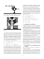
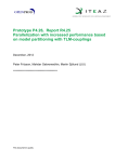
Figure 4. Pressure increases until the reference pressure of
10 MPa is reached, where the relief valve opens.
3.5e-06
Modelica tools also offer the possibility to use delays
instead of sampling. If you use delays, you end up with
continuous-time variables instead of discrete-time ones.
The methods are numerically very similar, but because the
variables are continuous when you use delay, the curve will
look smoother.
OpenModelica, ideal
OpenModelica, sample
OpenModelica, delay
Hopsan
3e-06
position of valve
2.5e-06
left.c = delay(right.c + 2 * Zc * right
.q, T);
right.c = delay(left.c + 2 * Zc * left.
q, T);
2e-06
1.5e-06
1e-06
5e-07
0
1
Finally, it is possible to explicitly specify a derivative
rather than obtaining it implicitly by difference computations relating to previous values (delays or sampling). This
then becomes a transmission line without delay, which is a
good reference system.
1.005
1.01
1.015
time
1.02
1.025
1.03
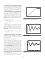
Figure 5. Comparison of spool position using different
TLM implementations.
der(left.p) = (left.q+right.q)/C;
der(right.p) = der(left.p);
1.002e+07
OpenModelica, ideal
OpenModelica, sample
OpenModelica, delay
Hopsan
1.0015e+07
1.001e+07
1.0005e+07
pressure
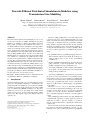
Figure 4 contains the results of simulating our example
system, i.e., the pressure relief valve from section 4. Figures 5 and 6 are magnified versions that show the difference
between our different TLM implementations. The models
used to create the Figures, are part of the Modelica package
DerBuiltin in Appendix A.
If you decrease the delay in the transmission even closer
to zero (it is now 10−4 ), the signals are basically the same
(as would be expected). It does however come at a significant increase in simulation times and decreased numerical
stability. This is not acceptable if stable real-time performance is desired. We use the same step size as the delay
of the transmission line since that is the maximum allowed
time step using this method, and better shows numerical
issues than a tiny step size.
Due to the nature of integrating solvers, we calculate
the value der(x), and use reinit() when der(x)
1e+07
9.995e+06
9.99e+06
9.985e+06
9.98e+06
1
1.005
1.01
1.015
1.02
1.025
time
Figure 6. Comparison of system pressure using different
TLM implementations.
75
3.5e-06
3e-06
OpenModelica, ideal
OpenModelica, sample
OpenModelica, delay
Hopsan
1.0015e+07
2.5e-06
1.001e+07
2e-06
1.0005e+07
pressure
position of valve
1.002e+07
OpenModelica, ideal
OpenModelica, sample
OpenModelica, delay
Hopsan
1.5e-06
1e+07
1e-06
9.995e+06
5e-07
9.99e+06
0
9.985e+06
-5e-07
9.98e+06
1
1.005
1.01
1.015
time
1.02
1.025
1.03
1
1.005
1.01
1.015
1.02
1.025
time
Figure 7. Comparison of spool position with inlined explicit euler.
Figure 8. Comparison of system pressure with inlined explicit euler.
Table 1. Performance comparison between different models in the DerBuiltin and DerInline packages.
Method
Builtin (sec) Inlined (sec)
OpenModelica Delay
0.13
0.40
OpenModelica Ideal
0.04
0.27
OpenModelica Sample
3.65
63.63
Dymola Ideal
0.64
0.75
Dymola Sample
1.06
1.15
The current OpenModelica simulation runtime system
implementation does not have special efficient implementations of time events or delayed expressions.
The inlined solver uses delay explicitly instead of being an actual inlined solver. This means it needs to search
an array for the correct value rather than accessing it directly, resulting in an overhead that will not exist once inline solvers are fully implemented in OpenModelica.
We used the -noemit flag in OpenModelica to disable
generation of result files. Generating them takes between
20% and 90% of total simulation runtime depending on
solver and if many events are generated.
Do not compare the current Dymola [6] performance
numbers to OpenModelica. We run Dymola inside a Windows virtual machine, while we run OpenModelica on
Linux.
The one thing that the performance numbers really tells
you is not to use sampling in OpenModelica until performance is improved, and that the overhead of inlining the
derivative using delay is a lot lower in Dymola than it is
in OpenModelica.
changes sign. The OpenModelica DASSL solver cannot be
used in all of these models due to an incompatibility with
the delay() operator (the solver does not limit its step
size as it should). DASSL is used together with sampling
since the solver does limit its step size if a zero crossing
occurs; in the other simulations the Euler solver is used.
Because of these reasons we tried to use another method
of solving the equation system, see package DerInline
in Appendix A. We simply inlined a derivative approximation (x-delay(x,T))/T instead of der(x), which is
much closer to the discrete-time approximation used in the
H OPSAN model. This is quite slow in practice because of
the overhead delay adds, but it does implicitly inline the
solver, which is a good property for in parallelization.
If you look at Figures 7 and 8, you can see that all simulations now have the same basic shape. In fact, the OpenModelica ones have almost the same values. The time step
is still 10−4 , which means you get the required behavior
even without sacrificing simulation times.
Even in this small example, the implementation using
delays has 1 state variable, while the ideal, zero-delay, implementation has 3 state variables. This makes it easier to
automatically parallelize larger models since the centralized solver handles fewer calculations. When inlining the
der() operator, we end up with 0 continuous-time state
variables.
Table 1 contains some performance numbers on the
models used. At this early stage in the investiagtion the
numbers are not that informative for several reasons.
We only made single-core simulations so far. Models
that have better parallelism will get better speedups when
we start doing multi-core simulations.
7.
Distributed Solver
The implementation using an inlined solver in Section 6
is essentially a distributed solver. It may use different time
steps in different submodels, which means a system can
be simulated using a very small time step only for certain
components. The advantage of such a distributed system
becomes apparent in [16].
In the current OpenModelica implementation this is not
yet taken advantage of, i.e., the states are solved in each
time step regardless.
8.
Related Work
Several people have performed work on parallelization of
Modelica models [2, 18, 19, 20, 23, 28], but there are still
many unsolved problems to address.
The work closest to this paper is [23], where Nyström
uses transmission lines to perform model partitioning for
parallelization of Modelica simulations using computer
clusters. The problem with clusters is the communication
76
overhead, which is huge if communication is performed
over a network. Real-time scheduling is also a bit hard to
reason about if you connect your cluster nodes through
TCP/IP. Today, there is an increasing need to parallelize
simulations on a single computer because most CPUs are
multi-core. One major benefit is communication costs; we
will be able to use shared memory with virtually no delay
in interprocessor communication.
Another thing that is different between the two implementations is the way TLM is modeled. We use regular
Modelica models without function calls for communication between model elements. Nyström used an external
function interface to do server-client communication. His
method is a more explicit way of parallelization, since he
looks for the submodels that the user created and creates a
kind of co-simulation.
Inlining solvers have also been used in the past to introduce parallelism in simulations [18].
9.
[1] The HOPSAN Simulation Program, User’s Manual.
Linköping University, 1985. LiTH-IKP-R-387.
[2] Peter Aronsson. Automatic Parallelization of EquationBased Simulation Programs. Doctoral thesis No 1022,
Linköping University, Department of Computer and Information Science, 2006.
[3] D. M. Auslander. Distributed System Simulation with
Bilateral Delay-Line Models. Journal of Basic Engineering,
Trans. ASME:195–200, 1968.
[4] Mikael Axin, Robert Braun, Petter Krus, Alessandro
dell’Amico, Björn Eriksson, Peter Nordin, Karl Pettersson,
and Ingo Staack. Next Generation Simulation Software
using Transmission Line Elements. In Proceedings of the
Bath/ASME Symposium on Fluid Power and Motion Control
(FPMC), Sep 2010.
[5] JD Burton, KA Edge, and CR Burrows. Partitioned
Simulation of Hydraulic Systems Using Transmission-Line
Modelling. In ASME WAM, 1993.
[6] Dassault Systèmes. Dymola 7.3, 2009.
Further Work
To progress further we need to introduce replace the use of
the delay() operator in the delay lines with an algorithm
section. This would make the initial equations easier to
solve, the system would simulate faster, and it would retain
the property that connected subsystems don’t depend on
each other.
Once we have partitioned a Modelica model into a distributed system model, we will be able to start simulating
the submodels in parallel, as described in [12, 16].
Some of the problems inherent in parallelization of
models expressed in EOO languages are solved by doing
this partitioning. By partitioning the model, you essentially
create many smaller systems, which are trivial to schedule
on multi-core systems.
To progress this work further a larger more computationally intensive model is also needed. Once we have a
good model and inlined solvers, we will work on making
sure that compilation and simulation scales well both with
the target number of processors and the size of the problem.
10.
References
Conclusions
We conclude that all implementations work fine in Modelica.
The delay line implementation using delays is not considerably slower than the one using the der() operator,
but can be improved by using for example algorithm sections here instead. Sampling also works fine, but is far too
slow for real-time applications. The delay implementation
should be preferred over using der(), since the delay will
partition the whole system into subsystems, which are easy
to parallelize.
Approximating integration by inline euler using the delay operator is not necessary to ensure stability although it
produces results that are closer to the results of the same
simulation in H OPSAN. When you view the simulation as a
whole, you can’t see any difference (Figure 4).
[7] Björn Eriksson, Peter Nordin, and Petter Krus. H OPSAN, A
C++ Implementation Utilising TLM Simulation Technique.
In Proceedings of the 51st Conference on Simulation and
Modelling (SIMS), October 2010.
[8] Peter Fritzson. Principles of Object-Oriented Modeling and
Simulation with Modelica 2.1. Wiley, 2004.
[9] Peter Fritzson, Peter Aronsson, Håkan Lundvall, Kaj
Nyström, Adrian Pop, Levon Saldamli, and David Broman.
The OpenModelica Modeling, Simulation, and Software
Development Environment. Simulation News Europe,
44/45, December 2005.
[10] Peter Fritzson et al. Openmodelica 1.5.0 system documentation, June 2010.
[11] Jason Howard et al. A 48-core IA-32 message-passing
processor with DVFS in 45nm CMOS. In Solid-State
Circuits Conference Digest of Technical Papers (ISSCC),
2010 IEEE International, pages 108 –109, 7-11 2010.
[12] Arne Jansson, Petter Krus, and Jan-Ove Palmberg. Real
Time Simulation Using Parallel Processing. In The 2nd
Tampere International Conference on Fluid Power, 1991.
[13] P. B. Johns and M. A. O’Brien. Use of the transmission
line modelling (t.l.m) method to solve nonlinear lumped
networks. The Radio and Electronic Engineer, 50(1/2):59–
70, 1980.
[14] David B. Kirk and Wen-Mei W. Hwu. Programming
Massively Parallel Processors: A Hands-On Approach.
Morgan Kaufmann Publishers, 2010.
[15] Petter Krus. Robust System Modelling Using Bi-lateral
Delay Lines. In Proceedings of the 2nd Conference on
Modeling and Simulation for Safety and Security (SimSafe),
Linköping, Sweden, 2005.
[16] Petter Krus, Arne Jansson, Jan-Ove Palmberg, and Kenneth
Weddfelt. Distributed Simulation of Hydromechanical
Systems. In The Third Bath International Fluid Power
Workshop, 1990.
[17] Air Force Aero Propulsion Laboratory. Aircraft hydraulic
system dynamic analysis. Technical report, Air Force Aero
77
Propulsion Laboratory, AFAPL-TR-76-43, Ohio, USA,
1977.
[18] Håkan Lundvall. Automatic Parallelization using Pipelining
for Equation-Based Simulation Languages. Licentiate thesis
No 1381, Linköping University, Department of Computer
and Information Science, 2008.
[19] Håkan Lundvall, Kristian Stavåker, Peter Fritzson, and
Christoph Kessler. Automatic Parallelization of Simulation
Code for Equation-based Models with Software Pipelining
and Measurements on Three Platforms. Computer Architecture News. Special Issue MCC08 – Multi-Core Computing,
36(5), December 2008.
[20] Martina Maggio, Kristian Stavåker, Filippo Donida,
Francesco Casella, and Peter Fritzson. Parallel Simulation of Equation-based Object-Oriented Models with
Quantized State Systems on a GPU. In Proceedings of the
7th International Modelica Conference, September 2009.
[21] Modelica Association. The Modelica Language Specification version 3.2, 2010.
[22] Modelica Association. Modelica Standard Library version
3.1, 2010.
[23] Kaj Nyström and Peter Fritzson. Parallel Simulation with
Transmission Lines in Modelica. In Christian Kral and
Anton Haumer, editors, Proceedings of the 5th International
Modelica Conference, volume 1, pages 325–331. Modelica
Association, September 2006.
[24] Thomas Rauber and Gudula Rünger. Parallel execution of
embedded and iterated runge-kutta methods. Concurrency Practice and Experience, 11(7):367–385, 1999.
[25] Alexander Siemers, Dag Fritzson, and Peter Fritzson. MetaModeling for Multi-Physics Co-Simulations applied for
OpenModelica. In Proceedings of International Congress
on Methodologies for Emerging Technologies in Automation
(ANIPLA), November 2006.
[26] Ryoji Tsuchiyama, Takashi Nakamura, Takuro Iizuka, Akihiro Asahara, and Satoshi Miki. The OpenCL Programming
Book. Fixstars Corporation, 2010.
[27] T. J. Viersma. Analysis, Synthesis and Design of Hydraulic
Servosystems and Pipelines. Elsevier Scientific Publishing
Company, Amsterdam, The Netherlands, 1980.
[28] Per Östlund. Simulation of Modelica Models on the
CUDA Architecture. Master’s thesis, Linköping University,
Department of Computer and Information Science, 2009.
A.
Pressure Relief Valve - Modelica Source
Code
package TLM
package Basic
connector Connector_Q
output Real p;
output Real q;
input Real c;
input Real Zc;
end Connector_Q;
connector Connector_C
input Real p;
input Real q;
output Real c;
output Real Zc;
end Connector_C;
model FlowSource
Connector_Q source;
parameter Real flowVal;
equation
source.q = flowVal;
source.p = source.c + source.q*
source.Zc;
end FlowSource;
model PressureSource
Connector_C pressure;
parameter Real P;
equation
pressure.c = P;
pressure.Zc = 0;
end PressureSource;
model HydrAltPRV
Connector_Q left;
Connector_Q right;
parameter Real Pref = 20000000;
parameter Real cq = 0.67;
parameter Real spooldiameter = 0.01;
parameter Real frac = 1.0;
parameter Real W = spooldiameter*frac
;
parameter Real pilotarea = 0.001;
parameter Real k = 1e6;
parameter Real c = 1000;
parameter Real m = 0.01;
parameter Real xhyst = 0.0;
constant Real xmax = 0.001;
constant Real xmin = 0;
parameter Real T;
parameter Real Fs = pilotarea*Pref;
Real Ftot = left.p*pilotarea - Fs;
Real Ks = cq*W*x;
Real x(start = xmin);
parameter Integer one = 1;
constant Boolean useDerInlineDelay;
Real xfrac = x*Pref/xmax;
Real v = if useDerInlineDelay then (
x-delay(x,T))/T else der(xtmp);
Real a = if useDerInlineDelay then (
v-delay(v,T))/T else der(v);
Real v2 = c*v;
Real x2 = k*x;
Real xtmp;
equation
left.p = left.c + left.Zc*left.q;
right.p = right.c + right.Zc*right.q;
left.q = -right.q;
right.q = sign(left.c-right.c) * Ks *
(sqrt(abs(left.c-right.c)+((
left.Zc+right.Zc)*Ks)^2/4) - Ks*(
left.Zc+right.Zc)/2);
xtmp = (Ftot - c*v - m*a)/k;
78
x = if noEvent(xtmp < xmin) then xmin
else if noEvent(xtmp > xmax)
then xmax else xtmp;
end HydrAltPRV;
end Basic;
package Continuous
extends Basic;
model Volume
parameter Real V;
parameter Real Be;
parameter Real Zc = Be*T/V;
parameter Real T;
Connector_C left(Zc = Zc);
Connector_C right(Zc = Zc);
equation
left.c = delay(right.c+2*Zc*right.q,T
);
right.c = delay(left.c+2*Zc*left.q,T)
;
end Volume;
end Continuous;
package ContinuousNoDelay
extends Basic;
model Volume
parameter Real V;
parameter Real Be;
parameter Real Zc = Be*T/V;
parameter Real T;
parameter Real C =V/Be;
Connector_C left(Zc = Zc);
Connector_C right(Zc = Zc);
protected
Real derleftp;
equation
derleftp = (left.q+right.q)/C;
derleftp = der(left.p);
derleftp = der(right.p);
end Volume;
end ContinuousNoDelay;
package Discrete
extends Basic;
model Volume
parameter Real V;
parameter Real Be;
parameter Real Zc = Be*T/V;
parameter Real T = 0.01;
Connector_C left(Zc = Zc);
Connector_C right(Zc = Zc);
equation
when sample(-T,T) then
left.c = pre(right.c)+2*Zc*pre(
right.q);
right.c = pre(left.c)+2*Zc*pre(
left.q);
end when;
end Volume;
end Discrete;
end TLM;
package BaseSimulations
constant Boolean useDerInlineDelay;
model HydrAltPRVSystem
replaceable model Volume =
TLM.Continuous.Volume;
parameter Real T = 1e-4;
Volume volume(V=1e-3,Be=1e9,T=T);
TLM.Continuous.FlowSource
flowSource(flowVal = 1e-5);
TLM.Continuous.PressureSource
pressureSource(P = 1e5);
TLM.Continuous.HydrAltPRV hydr(Pref
=1e7,cq=0.67,spooldiameter
=0.0025,frac=1.0,pilotarea=5
e-5,xmax=0.015,m=0.12,c=400,k
=150000,T=T,useDerInlineDelay=
useDerInlineDelay);
equation
connect(
flowSource.source,volume.left);
connect(volume.right,hydr.left);
connect(
hydr.right,pressureSource.pressure
);
end HydrAltPRVSystem;
model DelayDassl
extends HydrAltPRVSystem;
end DelayDassl;
model DelayEuler
extends HydrAltPRVSystem;
end DelayEuler;
model NoDelay
extends HydrAltPRVSystem(redeclare
model Volume =
TLM.ContinuousNoDelay.Volume);
end NoDelay;
model Disc
extends HydrAltPRVSystem(redeclare
model Volume =
TLM.Discrete.Volume);
end Disc;
end BaseSimulations;
package DerBuiltin
extends BaseSimulations(
useDerInlineDelay = false);
redeclare class extends
HydrAltPRVSystem
equation
when (hydr.v > 0) then
reinit(hydr.xtmp, max(
hydr.xmin,hydr.xtmp));
elsewhen (hydr.v < 0) then
reinit(hydr.xtmp, min(
hydr.xmax,hydr.xtmp));
end when;
end HydrAltPRVSystem;
end DerBuiltin;
package DerInline
79
extends BaseSimulations(
useDerInlineDelay = true);
end DerInline;
80