Download SBML Viewer User Manual

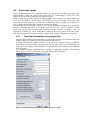
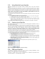
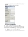
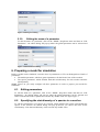
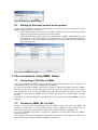
SBML Viewer User Manual
Laurent Francioli
[email protected]
Swiss Institute of Technology, 1015 Lausanne, Switzerland
March 10th, 2006
Version 1.0
Table of Contents
SBML Viewer User Manual.................................................................................................................... 1
Table of Contents .................................................................................................................................... 1
1. Introduction ..................................................................................................................................... 1
1.1.
The SBML Viewer window................................................................................................... 2
2. Prerequisites and installation........................................................................................................... 2
3. Launching and closing SBML Viewer ............................................................................................ 2
3.1.
Launching SBML Viewer...................................................................................................... 2
3.2.
Closing SBML Viewer .......................................................................................................... 2
4. Handling files using SBML Viewer ................................................................................................ 2
4.1.
Opening a file......................................................................................................................... 3
4.2.
Closing a file .......................................................................................................................... 3
4.3.
Saving a file ........................................................................................................................... 3
5. Graph layout .................................................................................................................................... 3
5.1.
Manual Layout ....................................................................................................................... 3
5.2.
Automatic layout.................................................................................................................... 4
5.2.1. Simulated Annealing Layout Algorithm ........................................................................... 4
5.2.2. Spring Embedded Layout Algorithm................................................................................. 5
5.2.3. Sugiyama Layout Algorithm ............................................................................................. 5
5.2.4. GEM Layout Algorithm .................................................................................................... 5
5.3.
Species, Reactions and parameters name editing................................................................... 6
5.3.1. Editing the name of a Species or a Reaction ..................................................................... 6
5.3.2. Editing the name of a parameter........................................................................................ 7
6. Preparing a model for simulation .................................................................................................... 7
6.1.
Editing parameters ................................................................................................................. 7
6.2.
Specifying the stoichiometry of a species in a reaction ......................................................... 7
6.3.
Setting up the initial amount of the species ........................................................................... 8
7. File conversions using SBML Viewer ............................................................................................ 8
7.1.
Converting a TSed file to SBML ........................................................................................... 8
7.2.
Convert an SBML file to LaTeX ........................................................................................... 8
7.3.
Export the SBML Model to a Matlab file for simulation....................................................... 9
8. More about SBML Viewer and its framework................................................................................ 9
9. References ....................................................................................................................................... 9
1. Introduction
SBML Viewer is a java application to display and work on biological networks in the Systems
Biology Markup Language (SBML) format. It is part of the Bio-Chemical Modelling Tools framework
that provides tools to describe, represent and simulate networks of biological interactions.
This user manual explains how to use SBML Viewer to efficiently display biological network models
and work with them.
1.1. The SBML Viewer window
Figure 1 shows an empty SBML Viewer window and its main components.
Figure 1: SBML Viewer window
2. Prerequisites and installation
Since SBML Viewer is written in Java, it requires Java 1.4 or higher to be installed.
The installation of SBML Viewer is rather simple and is explained in the user manual of the
framework available on the world wide web at: http://lcawww.epfl.ch ; please refer to it to install
SBML Viewer.
3. Launching and closing SBML Viewer
3.1. Launching SBML Viewer
Once installed, go in the directory you installed SBML Viewer in and simply run the executable file.
Under Linux, run SView by typing “./SView” to launch SBML Viewer. Under windows, double-click
on SView.bat to launch SBML Viewer.
3.2. Closing SBML Viewer
To close SBML Viewer, either double-click on the cross at the top-right of the SBML Viewer
windows or go use the drop-down menu File and click on Exit.
Please note that SBML Viewer does not automatically save your work on exit.
4. Handling files using SBML Viewer
SBML Viewer gives a graphical representation of SBML files. It only supports the SBML format, but
features an easy link with TSed2SBML to convert TSed [1] files to SBML in order to use them as
well. See section 7.1 about how to convert a TSed file to SBML.
4.1. Opening a file
To open a file, click on the “Open” button of the “File” drop-down menu. A file chooser will pop
up and let you choose the file to open. Once a file is opened its graph is automatically displayed.
Please note that only SBML files are supported.
4.2. Closing a file
To close a file, click on the “Close” button of the “File” drop-down menu. Please note that SBML
Viewer does not automatically save your work before closing a file.
4.3. Saving a file
If you want to save the changes made to a file, click on the “Save” button of the “File” drop-down
menu.
If you want to save the file with its changes under a new file, click on the “Save As…” button of
the “File” drop-down menu. A file chooser will then pop up and let you choose where you want to
save your file and what name you want it to have. Please note that SBML Viewer won’t add the
extension for you; therefore to save it using the standard SBML extension, save it with the .xml
extension.
5. Graph layout
Once an SBML file is opened, its graph will be displayed. Depending on whether it already contains
information relative to its display or not, the graph will be either nicely displayed or all shrunk in the
upper left corner of SBML Viewer. To nicely layout the graph, you will probably have to first use one
or more of the automatic layout algorithms and then finish the layout manually.
5.1. Manual Layout
To manually layout part of a graph, simply drag and drop any reaction or species anywhere on the
screen.
The size of each cell can also be adjusted. To do so, first select a cell by clicking on it. Then hold
the left mouse button pressed on one of the 8 anchors of the cell and drag it until the desired size is
obtained. When dragging the anchor, SBML Viewer displays a shadow representing the new size
of the cell. Note that the mouse shape changes into a double-headed arrow when hovering over an
anchor.
Figure 2: Resizing of a Cell
5.2. Automatic layout
The use of automatic layout can considerably reduce the layout time of a graph by providing a first
approximation of what the graph of the model looks like. Unfortunately in most cases some
manual work will still be needed after the automatic layout.
SBML Viewer proposes four automatic layout algorithms. They can work very well by themselves
or be used in parallel for better results. The sections 5.2.1 to 5.2.3 briefly present these four
algorithms and their parameters. To efficiently automatically layout a graph it is imperative to
have a rough understanding of the algorithms and their parameters.
All automatic layout algorithms, except for the spring embedded algorithm, are configurable
through a configuration dialog. To reach this dialog: click on the “Layout” drop-down menu,
scroll down on the name of the desired algorithm and then click on “Configure”. Once an
algorithm is configured, it can be launched by clicking on the “Run” button of the same menu.
Note that if an algorithm is launched without configuration, a default configuration is provided.
5.2.1.
Simulated Annealing Layout Algorithm
The simulated annealing layout algorithm is implemented from the work of R.Davidson and
D.Harel, "Drawing Graphs Nicely Using Simulated Annealing" [2].
Its output minimizes the number of edges crossings but doesn’t penalize vertices overlapping.
Thus results in a good looking graph requiring few user works afterwards. Unfortunately the
algorithm is very complex and requires lots of computing time, thus making it a bad candidate
for large graphs.
The simulated annealing algorithm has 15 parameters configurable through a configuration
dialog. Please see [2] for a description of the algorithm and its parameters.
Figure 3: Simulated Annealing Layout Algorithm Configuration Dialog
5.2.2.
Spring Embedded Layout Algorithm
The spring embedded layout algorithm available in SBML Viewer is the work of S.Luzar
[REF].
The spring embedded layout algorithm is very good at separating sub graphs from a complex
graph and at separating strongly connected regions of a graph in general. Its solution comport
minimum vertices overlapping but can result in extra edges crossings. Distances in between
vertices of the strongly connected regions of the graph are usually small and therefore the
output usually is too compact. To correct this default, a good solution is to use it in
conjunction with the GEM layout algorithm.
This algorithm works fast and well, even for large graphs, but requires some user works after
completion.
The spring embedded algorithm is iterative and works by:
ƒ Considering every edge like a spring that tends to get its two connected cells together
ƒ Considering that every vertex repulses the other vertices.
ƒ Each iteration: calculating the forces between that attract the connected vertices
together and the forces that repulse the vertices from each other and moving the
vertices accordingly to these forces.
The algorithm works iteratively and only requires one parameter: the number of iterations.
5.2.3.
Sugiyama Layout Algorithm
The sugiyama layout algorithm is based on the work of K.Sugiyama and P.Eades: “How to
draw a directed graph” [4].
The sugiyama layout algorithm is quick and good at separating sub graphs from a complex
model. It is therefore highly recommended to use it when the model is composed of a number
of small graphs. The output of this algorithm is quite well spaced. Unfortunately all the
entities of a reaction are linearly aligned without caring for edges crossing vertices, which
often leads to confusing representations. Nonetheless it is a very powerful algorithm that can
eventually be applied to first space out the graph before applying other algorithms.
The sugiyama layout algorithm works by spreading out the graph, laying the vertices linearly
on one dimension if connected and in the other dimension if not. The algorithm has only 4
parameters configurable through a configuration dialog:
ƒ Horizontal Spacing: the spacing desired horizontally between two vertices
ƒ Vertical Spacing: the spacing desired vertically between two vertices
ƒ Vertical Orientation: If selected, the connected vertices will be laid vertically and the
non-connected vertices horizontally. If not selected, the connected vertices will be laid
horizontally and the non-connected vertices vertically.
ƒ Flush to Origin: If selected, the first group of connected vertices will be shifted to the
top-left corner of SBML Viewer.
For further information about the sugiyama algorithm and its parameters, please see [4].
Figure 4: Sugiyama Layout Algorithm Configuration Dialog
5.2.4.
GEM Layout Algorithm
The GEM layout algorithm is based on the work of A.Frick, A.Ludwig, H.Mehldau: "A Fast
Adaptive Layout Algorithm for Undirected Graphs" [3].
Its output is a graph with few vertices overlapping and - although the algorithm doesn’t
explicitly minimize it – reasonable edges crossings.
Its downside is that it tends to output very spread out graphs; therefore combining this
algorithm with the spring embedded is a great solution to automatically layout large and
complex graphs.
The GEM Layout Algorithm has 16 parameters configurable through a configuration dialog.
Please see [3] for a description of the algorithm and its parameters.
Figure 5: GEM Layout Algorithm Configuration Dialog
5.3. Species, Reactions and parameters name editing
Since a graph aims to represent a model in an easily understandable way, the naming of its entities
is also important. Therefore, SBML Viewer proposes tools to easily edit the names of the species,
reactions and parameters of a model. Since SBML Viewer always stays consistent with SBML2,
the names of these entities have to follow the SBML2 guidelines [5]. Especially a name is unique
among the model in order to prevent naming ambiguities.
5.3.1.
Editing the name of a Species or a Reaction
To change the name of a reaction or a species, simply double-click on its cell representation in
the graph. An edition dialog will then pop up where you can edit its name.
Figure 6: Edit Species Dialog
5.3.2.
Editing the name of a parameter
To edit the name of a parameter, click on the “SBML” drop-down menu and then on “Edit
Parameters”. An edition dialog will pop up where the global parameters can be selected and
edited.
Figure 7: Edit Parameters Dialog
6. Preparing a model for simulation
Before a model can be simulated, it needs to have its parameters set. We can distinguish two kinds of
parameters:
ƒ The models parameter, which are general parameters for the kinetic laws of the reactions.
ƒ The species parameters, which includes both their stoichiometry for each reaction and their
initial quantity.
SBML Viewer let you easily configure all these parameters in order to prepare your model for
simulation.
6.1. Editing parameters
To edit the name of a parameter, click on the “SBML” drop-down menu and then on “Edit
Parameters”. An edition dialog will pop up where the global parameters can be selected and
edited. Note that the model’s parameters can take any double value. See figure Figure 7.
6.2. Specifying the stoichiometry of a species in a reaction
To edit the stoichiometry of a species in a reaction, simply double-click on the edge binding the
species to the reaction. An edition dialog will pop up and let you choose the value of the
stoichiometry. Note that stoichiometry values can take any double value.
Figure 8: Stoichiometry Edititon Dialog
6.3. Setting up the initial amount of the species
To successfully simulate a model, the initial amount of every species has to be specified. To do so
SBML Viewer provides two interfaces:
ƒ Set the initial amount of one species by double-clicking on its cell in the graph. An edition
dialog will pop up and let you specify its initial amount.
ƒ Set the initial amount of all the species by clicking on the “SBML” menu and then on “Set
Concentrations”. An edition dialog will pop up and let you change the initial amount of
any species in a table. This option is convenient is you have to set the initial amount for
many species at once.
Figure 9: Set Concentrations Dialog
7. File conversions using SBML Viewer
7.1. Converting a TSed file to SBML
Converting a TSed file to SBML let you then display this file using SBML Viewer, prepare it for
simulation and then convert it to a Matlab file for simulation.
To convert a TSed file to SBML, click on the “Translate a TSed file to SBML” from the “SBML”
drop-down menu. A file chooser will pop up and let you select the TSed file you want to convert.
Once chosen, the file is converted to SBML and saved under the same name as the selected TSed
file with the .xml extension. SBML Viewer will then ask the user if it should display its graph
directly.
Note that if you choose to display the graph, it will close any other opened file without saving its
changes.
7.2. Convert an SBML file to LaTeX
Thanks to a built-in link with SBML2LaTeX [6], SBML Viewer can convert the SBML file
opened to a LaTeX file. It can be greatly useful to convert a SBML file into LaTeX since it is
easier to read and gives a good textual resume of the model described by the SBML file.
To convert an SBML file to LaTeX, click on the “Translate to LaTeX” button from the “SBML”
drop-down menu.
Once clicked, two files are automatically generated in the directory of the opened file. These files
both have the name of the opened file but different extensions:
ƒ
ƒ
The first file has a .tex extension and is a LaTeX file describing the SBML model of the
opened file.
The second file has a .sh extension and will compile the .tex file into a PDF file if run.
7.3. Export the SBML Model to a Matlab file for simulation
Once your model is ready for simulation, you will need to export it into a Matlab simulation file.
Thanks to a built-in link with SBML2Matlab [6], this can be done directly from SBML Viewer.
To export the opened file into a Matlab simulation file, click on the “Export to Matlab” button
from thw “SBML” drop-down menu. Once clicked, SBML Viewer will automatically generate
two files. These files can be found in the same directory as the opened file.
ƒ The first file has the same name as the opened file and has a .m extension. This file
contains the SBML model translated into a Matlab structure and Matlab ODEs.
ƒ The second file is named like the opened file + “_simulate” and has a .m extension. This
file contains basic simulation commands using the first file.
Please note that it is important to set up the parameters of your model and the initial quantities of
every species before exporting your model for simulation. See section REF to do so.
8. More about SBML Viewer and its framework
To find out more about how to SBML Viewer within the bio-chemical modelling tools network and
the LCA research group, visit our website at: lcawww.epfl.ch.
9. References
[1] M. Sede (2006). “Fast Chemical Reactions Modeling with TSed”. Available on the World Wide
Web at: http://lcawww.epfl.ch
[2] R. Davidson, D. Harel. “Drawing graphs nicely using simulated annealing” (1996). ACM
Transactions on Graphing (TOG), Volume 15, Issue 4, pp. 301-331. ACM Press, New-York, USA
[3] A.Frick, A.Ludwig, H.Mehldau (1994). "A Fast Adaptive Layout Algorithm for Undirected
Graphs". Proceedings of the DIMACS International Workshop on Graph Drawing, pp. 388-403,
Springer-Verlag, London, UK
[4] K.Sugiyama, P.Eades (1991). “How to draw a directed graph”. Journal of Information Processing,
volume 13, issue 4, pp.424-437. Processing Society of Japan, Tokyo, Japan.
[5] A.Finney, M.Hucka (2003). “Systems Biology Markup Language (SBML) Level 2: Structures and
Facilities for Model Definitions”. California Institute of Technology, Pasadena, USA
[6] . Eperon (2006). “On modelling a bio-chemical process, from models to simulation”. Available on
the World Wide Web at: http://lcawww.epfl.ch