Download Linux® Application Tuning Guide for SGI® X86

Linux Application Tuning Guide for SGI
X86-64 Based Systems
®
007–5646–007
®
COPYRIGHT
© 2010–2014, SGI. All rights reserved; provided portions may be copyright in third parties, as indicated elsewhere herein. No
permission is granted to copy, distribute, or create derivative works from the contents of this electronic documentation in any manner,
in whole or in part, without the prior written permission of SGI.
LIMITED RIGHTS LEGEND
The software described in this document is "commercial computer software" provided with restricted rights (except as to included
open/free source) as specified in the FAR 52.227-19 and/or the DFAR 227.7202, or successive sections. Use beyond license provisions is
a violation of worldwide intellectual property laws, treaties and conventions. This document is provided with limited rights as defined
in 52.227-14.
TRADEMARKS AND ATTRIBUTIONS
Altix, ICE, NUMAlink, OpenMP, Performance Co-Pilot, SGI, the SGI logo, SHMEM, and UV are trademarks or registered trademarks
of Silicon Graphics International Corp. or its subsidiaries in the United States and other countries.
Cray is a registered trademark of Cray, Inc. Dinkumware is a registered trademark of Dinkumware, Ltd. Intel, GuideView, Itanium,
KAP/Pro Toolset, Phi, VTune, and Xeon are trademarks or registered trademarks of Intel Corporation, in the United States and other
countries. Oracle and Java are registered trademarks of Oracle and/or its affiliates. Linux is a registered trademark of Linus Torvalds
in several countries. Red Hat and Red Hat Enterprise Linux are registered trademarks of Red Hat, Inc., in the United States and other
countries. PostScript is a trademark of Adobe Systems Incorporated. SUSE is a registered trademark of SUSE LLC in the United States
and other countries. TotalView and TotalView Technologies are registered trademarks and TVD is a trademark of Rogue Wave
Software, Inc. Windows is a registered trademark of Microsoft Corporation in the United States and/or other countries. All other
trademarks are the property of their respective owners.
New Features
This revision includes the following updates:
• Removed references to the Unified Parallel C (UPC) product.
• Revised chapter 5, Data Placement Tools for SGI UV Computers
• Added information about the madvise keyword for transparent huge pages.
• Miscellaneous editorial and technical corrections.
007–5646–007
iii
Record of Revision
007–5646–007
Version
Description
001
November 2010
Original publication.
002
February 2011
Supports the SGI Performance Suite 1.1 release.
003
November 2011
Supports the SGI Performance Suite 1.3 release.
004
May 2012
Supports the SGI Performance Suite 1.4 release.
005
November 2013
Supports the SGI Performance Suite 1.7 release.
006
November 2013
Supports the SGI Performance Suite 1.7 release and includes a
correction to the PerfSocket installation documentation.
007
May 2014
Supports the SGI Performance Suite 1.8 release.
v
Contents
About This Guide
. . . .
Related SGI Publications
.
.
.
. . . .
.
.
Related Publications From Other Sources
. . .
. . . .
. . . .
. .
xiii
.
.
.
.
.
.
.
.
.
.
.
.
.
.
.
.
xiii
.
.
.
.
.
.
.
.
.
.
.
.
.
.
.
.
xv
Obtaining Publications
.
.
.
.
.
.
.
.
.
.
.
.
.
.
.
.
.
.
.
.
.
.
xvi
Conventions
.
.
.
.
.
.
.
.
.
.
.
.
.
.
.
.
.
.
.
.
.
.
.
xvi
.
.
.
.
.
.
.
.
.
.
.
.
.
.
.
.
.
.
.
.
.
.
.
xvi
. . . .
. .
1
.
.
Reader Comments
1. System Overview
. . .
. . . .
An Overview of SGI System Architecture
The Basics of Memory Management
.
.
Environment Modules
. . . .
.
.
.
.
.
.
.
.
.
.
.
.
.
.
.
.
1
.
.
.
.
.
.
.
.
.
.
.
.
.
.
.
.
1
. . . .
. .
3
2. The SGI Compiling Environment
Compiler Overview
. . .
.
. . .
. . . .
.
.
.
.
.
.
.
.
.
.
.
.
.
.
.
.
.
.
.
.
.
.
3
.
.
.
.
.
.
.
.
.
.
.
.
.
.
.
.
.
.
.
.
.
.
4
Library Overview
.
.
.
.
.
.
.
.
.
.
.
.
.
.
.
.
.
.
.
.
.
.
.
5
Static Libraries
.
.
.
.
.
.
.
.
.
.
.
.
.
.
.
.
.
.
.
.
.
.
.
6
.
.
.
.
.
.
.
.
.
.
.
.
.
.
.
.
.
.
.
.
.
.
6
.
.
.
.
.
.
.
.
.
.
.
.
.
.
.
.
.
.
.
.
.
.
6
.
.
.
.
.
.
.
.
.
.
.
.
.
.
.
.
.
7
. . . .
. .
9
Dynamic Libraries
C/C++ Libraries
.
SHMEM Message Passing Libraries
3. Performance Analysis and Debugging
. . .
. . . .
Determining System Configuration
.
.
.
.
.
.
.
.
.
.
.
.
.
.
.
.
.
.
9
Sources of Performance Problems
.
.
.
.
.
.
.
.
.
.
.
.
.
.
.
.
.
.
17
Profiling with perf
.
.
.
.
.
.
.
.
.
.
.
.
.
.
.
.
.
.
.
.
.
17
Profiling with PerfSuite
.
.
.
.
.
.
.
.
.
.
.
.
.
.
.
.
.
.
.
.
17
007–5646–007
.
vii
Contents
Other Performance Analysis Tools
About Debugging
.
.
.
Using the Intel Debugger
Using TotalView
.
.
.
.
.
.
.
.
.
.
.
.
.
.
.
.
.
.
.
.
.
18
.
.
.
.
.
.
.
.
.
.
.
.
.
.
.
.
.
.
.
.
19
.
.
.
.
.
.
.
.
.
.
.
.
.
.
.
.
.
.
.
.
20
.
.
.
.
.
.
.
.
.
.
.
.
.
.
.
.
.
.
.
.
21
.
.
.
.
.
.
.
.
.
.
.
.
.
.
.
.
.
22
. . . .
. .
25
Using the Data Display Debugger
4. Monitoring Tools
System Monitoring Tools
. . .
.
.
.
. . . .
.
.
.
.
Hardware Inventory and Usage Commands
. . .
. . . .
.
.
.
.
.
.
.
.
.
.
.
.
.
.
25
.
.
.
.
.
.
.
.
.
.
.
.
.
.
25
topology(1) Command
.
.
.
.
.
.
.
.
.
.
.
.
.
.
.
.
.
.
.
25
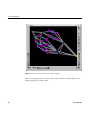
gtopology(1) Command
.
.
.
.
.
.
.
.
.
.
.
.
.
.
.
.
.
.
.
26
Performance Co-Pilot Monitoring Tools
.
.
.
.
.
.
.
.
.
.
.
.
.
.
.
.
29
hubstats(1) Command
.
linkstat-uv(1) Command
.
.
.
.
.
.
.
.
.
.
.
.
.
.
.
.
.
.
30
.
.
.
.
.
.
.
.
.
.
.
.
.
.
.
.
.
.
30
.
.
.
.
.
.
.
.
.
.
.
.
.
30
Other Performance Co-Pilot Monitoring Tools
System Usage Commands
.
.
.
.
.
.
.
.
.
.
.
.
.
.
.
.
.
.
.
.
32
.
.
.
.
.
.
.
.
.
.
.
.
.
.
.
.
.
.
.
.
32
Using the ps(1) Command
.
.
.
.
.
.
.
.
.
.
.
.
.
.
.
.
.
.
.
33
.
.
.
.
.
.
.
.
.
.
.
.
.
.
.
.
.
.
34
Using the vmstat(8) Command
.
.
.
.
.
.
.
.
.
.
.
.
.
.
.
.
.
34
Using the iostat(1) command
.
.
.
.
.
.
.
.
.
.
.
.
.
.
.
.
.
34
.
.
.
.
.
.
.
.
.
.
.
.
.
.
.
.
.
35
.
.
.
.
.
.
.
.
.
.
.
.
.
.
36
. . . .
. .
39
Using the w command
Using the top(1) Command
Using the sar(1) command
.
Memory Statistics and nodeinfo Command
5. Data Process and Placement Tools
.
. . .
About Nonuniform Memory Access (NUMA) Computers
Distributed Shared Memory (DSM)
ccNUMA Architecture
viii
.
.
.
.
. . . .
.
.
.
.
.
.
.
.
.
.
.
39
.
.
.
.
.
.
.
.
.
.
.
.
.
.
.
.
.
40
.
.
.
.
.
.
.
.
.
.
.
.
.
.
.
.
.
40
007–5646–007
®
®
Linux Application Tuning Guide for SGI X86-64 Based Systems
Cache Coherency
.
.
.
.
.
.
.
.
.
.
.
.
.
.
.
.
40
Non-uniform Memory Access (NUMA)
.
.
.
.
.
.
.
.
.
.
.
.
.
.
.
41
About the Data and Process Placement Tools
.
.
.
.
.
.
.
.
.
.
.
.
.
.
.
41
cpusets and cgroups
.
.
.
.
.
.
.
.
.
.
.
.
.
.
.
.
.
.
.
.
.
.
.
.
.
.
.
43
.
.
.
.
.
.
.
.
.
.
.
.
.
.
.
.
.
.
.
.
.
44
omplace Command
.
.
.
.
.
.
.
.
.
.
.
.
.
.
.
.
.
.
.
.
.
50
taskset Command
.
.
.
.
.
.
.
.
.
.
.
.
.
.
.
.
.
.
.
.
.
51
numactl Command
.
.
.
.
.
.
.
.
.
.
.
.
.
.
.
.
.
.
.
.
.
53
.
.
.
.
.
.
.
.
.
.
.
.
.
.
.
.
.
.
.
.
.
53
. . . .
. .
61
dplace Command
.
dlook Command
.
6. Performance Tuning
. .
About Performance Tuning
.
. . . .
. . .
. . . .
.
.
.
.
.
.
.
.
.
.
.
.
.
.
.
.
.
.
.
61
Single Processor Code Tuning
.
.
.
.
.
.
.
.
.
.
.
.
.
.
.
.
.
.
.
62
Getting the Correct Results
.
.
.
.
.
.
.
.
.
.
.
.
.
.
.
.
.
.
.
62
.
.
.
.
.
.
.
.
.
.
.
.
.
.
.
.
63
Managing Heap Corruption Problems
Using Tuned Code
.
.
.
Determining Tuning Needs
.
.
.
.
.
.
.
.
.
.
.
.
.
.
.
.
.
.
.
63
.
.
.
.
.
.
.
.
.
.
.
.
.
.
.
.
.
.
.
64
.
.
.
.
.
.
.
.
.
.
.
.
.
.
.
64
Using Compiler Options Where Possible
Tuning the Cache Performance
Managing Memory
.
.
Memory Use Strategies
Data Decomposition
.
.
Parallelizing Your Code
Use MPT
Use OpenMP
.
.
.
.
.
.
.
.
.
.
.
.
.
.
.
.
.
67
.
.
.
.
.
.
.
.
.
.
.
.
.
.
.
.
.
.
.
69
.
.
.
.
.
.
.
.
.
.
.
.
.
.
.
.
.
.
.
.
70
.
.
.
.
.
.
.
.
.
.
.
.
.
.
.
.
.
.
70
.
.
.
.
.
.
.
.
.
.
.
.
.
.
.
.
.
.
.
.
71
.
.
.
.
.
.
.
.
.
.
.
.
.
.
.
.
.
.
.
.
71
.
.
.
.
.
.
.
.
.
.
.
.
.
.
.
.
.
.
.
.
72
.
.
.
.
.
.
.
.
.
.
.
.
.
.
.
.
.
.
.
.
.
.
.
73
.
.
.
.
.
.
.
.
.
.
.
.
.
.
.
.
.
.
.
.
.
.
.
73
.
.
.
.
.
.
.
.
.
.
.
.
.
.
.
.
.
.
74
OpenMP Nested Parallelism
007–5646–007
.
.
Memory Hierarchy Latencies
Multiprocessor Code Tuning
.
ix
Contents
Use Compiler Options
.
.
.
.
.
.
.
.
.
Identifying Parallel Opportunities in Existing Code
Fixing False Sharing
.
.
.
.
.
.
.
.
.
Environment Variables for Performance Tuning
.
.
.
.
.
.
.
.
.
.
74
.
.
.
.
.
.
.
.
.
.
.
75
.
.
.
.
.
.
.
.
.
.
.
.
.
75
.
.
.
.
.
.
.
.
.
.
.
.
.
76
.
.
.
.
.
.
.
.
.
.
.
.
77
Understanding Parallel Speedup and Amdahl’s Law
Adding CPUs to Shorten Execution Time
.
.
.
.
.
.
.
.
.
.
.
.
.
.
.
.
78
.
.
.
.
.
.
.
.
.
.
.
.
.
.
.
.
78
.
.
.
.
.
.
.
.
.
.
.
.
.
.
.
.
79
.
.
.
.
.
.
.
.
.
.
.
.
.
.
.
.
79
Calculating the Parallel Fraction of a Program
.
.
.
.
.
.
.
.
.
.
.
.
.
.
80
Predicting Execution Time with n CPUs
.
.
.
.
.
.
.
.
.
.
.
.
.
.
.
81
Understanding Parallel Speedup
.
.
Understanding Superlinear Speedup
Understanding Amdahl’s Law
Gustafson’s Law
.
.
.
.
.
.
.
.
Floating-point Program Performance
About MPI Application Tuning
.
.
.
.
.
.
.
.
.
.
.
.
.
.
.
.
.
.
.
.
82
.
.
.
.
.
.
.
.
.
.
.
.
.
.
.
.
.
83
.
.
.
.
.
.
.
.
.
.
.
.
.
.
.
.
.
83
.
.
.
.
.
.
.
.
.
.
.
.
84
MPI Application Communication on SGI Hardware
MPI Job Problems and Application Design
.
.
.
.
.
.
.
.
.
.
.
.
.
.
.
84
MPI Performance Tools
.
.
.
.
.
.
.
.
.
.
.
.
.
.
.
86
.
.
.
.
.
.
87
.
.
.
88
. . . .
. .
89
.
.
.
.
.
.
Using Transparent Huge Pages (THPs) in MPI and SHMEM Applications
Enabling Huge Pages in MPI and SHMEM Applications on Systems Without THP
7. Flexible File I/O
FFIO Operation
.
. . . .
. . . .
. . .
. . . .
.
.
.
.
.
.
.
.
.
.
.
.
.
.
.
.
.
.
.
.
.
.
.
89
Environment Variables
.
.
.
.
.
.
.
.
.
.
.
.
.
.
.
.
.
.
.
.
.
.
90
Simple Examples
.
.
.
.
.
.
.
.
.
.
.
.
.
.
.
.
.
.
.
.
.
.
91
.
.
.
.
.
.
.
.
.
.
.
.
.
.
.
.
.
.
.
94
.
Multithreading Considerations
Application Examples
Event Tracing
x
.
.
.
.
.
.
.
.
.
.
.
.
.
.
.
.
.
.
.
.
.
.
.
.
95
.
.
.
.
.
.
.
.
.
.
.
.
.
.
.
.
.
.
.
.
.
.
96
007–5646–007
®
®
Linux Application Tuning Guide for SGI X86-64 Based Systems
System Information and Issues
8. I/O Tuning
. .
.
.
. . . .
.
.
.
.
. . . .
Application Placement and I/O Resources
.
.
.
. . .
.
.
.
.
.
.
. . . .
.
.
.
.
.
.
96
. . . .
. .
97
.
.
.
.
.
.
.
.
.
.
.
.
97
Layout of Filesystems and XVM for Multiple RAIDs
.
.
.
.
.
.
.
.
.
.
.
.
98
9. Suggested Shortcuts and Workarounds
. .
. . . .
. .
99
Determining Process Placement
.
.
. . . .
.
.
.
.
.
.
.
.
.
.
.
.
.
.
.
.
.
.
.
99
Example Using pthreads
.
.
.
.
.
.
.
.
.
.
.
.
.
.
.
.
.
.
.
.
100
Example Using OpenMP
.
.
.
.
.
.
.
.
.
.
.
.
.
.
.
.
.
.
.
.
102
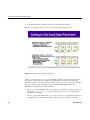
Combination Example (MPI and OpenMP)
.
.
.
.
.
.
.
.
.
.
.
.
.
.
.
104
.
.
.
.
.
.
.
.
.
.
.
.
.
.
.
106
.
.
.
.
.
.
.
.
.
.
.
.
.
.
.
107
Resetting System Limits
.
.
.
.
.
.
Resetting the File Limit Resource Default
Resetting the Default Stack Size
.
.
.
.
.
.
.
.
.
.
.
.
.
.
.
.
.
.
109
Avoiding Segmentation Faults
.
.
.
.
.
.
.
.
.
.
.
.
.
.
.
.
.
.
109
Resetting Virtual Memory Size
.
.
.
.
.
.
.
.
.
.
.
.
.
.
.
.
.
.
111
Linux Shared Memory Accounting
.
.
.
.
.
.
.
.
.
.
.
.
.
.
.
.
.
.
112
.
.
.
.
.
.
.
.
.
.
.
.
.
.
.
.
113
.
.
.
.
.
.
.
.
.
.
.
.
.
.
.
.
114
. . . .
. .
117
OFED Tuning Requirements for SHMEM
Setting Java Enviroment Variables
10. Using PerfSocket
About SGI PerfSocket
.
.
. . .
.
.
Installing and Using PerfSocket
.
. . . .
. . .
.
.
.
.
.
.
.
.
.
.
.
.
.
.
.
.
.
.
.
117
.
.
.
.
.
.
.
.
.
.
.
.
.
.
.
.
.
.
.
117
.
.
.
.
.
.
.
.
.
.
.
.
.
118
Installing PerfSocket (Adminstrator Procedure)
Running an Application With PerfSocket
About Security When Using PerfSocket
Troubleshooting
007–5646–007
.
.
.
.
.
. . . .
.
.
.
.
.
.
.
.
.
.
.
.
.
.
.
.
.
.
119
.
.
.
.
.
.
.
.
.
.
.
.
.
.
.
.
120
.
.
.
.
.
.
.
.
.
.
.
.
.
.
.
.
120
xi
Contents
Index
xii
.
. . . .
. . . .
. . . .
. . .
. . . .
. . . .
. .
121
007–5646–007
About This Guide
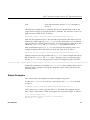
This publication provides information about how to tune C and Fortran application
programs that you compiled with an Intel compiler on an SGI® UVTM series system
that hosts either the Red Hat Enterprise Linux (RHEL) or the SUSE Linux Enterprise
Server (SLES) operating system. Some parts of this manual are also applicable to other
SGI X86-64 based systems, such as the SGI® ICETM X and SGI® RackableTM systems.
This guide is written for experienced programmers who are familiar with Linux
commands and with either the C or Fortran programming languages. The focus in this
document is on achieving the highest possible performance by exploiting the features
of your SGI system. The material assumes that you know the basics of software
engineering and that you are familiar with standard methods and data structures. If
you are new to programming or software design, this guide will not be of use to you.
Related SGI Publications
The release notes for the SGI Foundation Suite and the SGI Performance Suite list SGI
publications that pertain to the specific software packages in those products. The
release notes reside in a text file in the /docs directory on the product media. For
example, SGI-MPI-1.x-readme.txt. After installation, the release notes and other
product documentation reside in the /usr/share/doc/packages/product directory.
All SGI publications are available on the Technical Publications Library at
http://docs.sgi.com. The following publications provide information about Linux
implementations on SGI systems:
• SGI UV System Software Installation and Configuration Guide
Explains how to install the operating system on an SGI UV system. This manual
also includes information about basic configuration features such as CPU
frequency scaling and partitioning.
• SGI Cpuset Software Guide
Explains how to use cpusets within your application program. Cpusets restrict
processes within a program to specific processors or memory nodes.
• Message Passing Toolkit (MPT) User Guide
007–5646–007
xiii
About This Guide
Describes the industry-standard message passing protocol optimized for SGI
computers. This manual describes how to tune the run-time environment to
improve the performance of an MPI message passing application on SGI
computers. The tuning methods do not involve application code changes.
• MPInside Reference Guide
Documents the SGI MPInside MPI profiling tool.
• SGI hardware documentation.
SGI creates hardware manuals that are specific to each product line. The hardware
documentation typically includes a system architecture overview and describes the
major components. It also provides the standard procedures for powering on and
powering off the system, basic troubleshooting information, and important safety
and regulatory specifications.
The following procedure explains how to retrieve a list of hardware manuals for
your system.
Procedure 0-1 To retrieve hardware documentation
1. Type the following URL into the address bar of your browser:
docs.sgi.com
2. In the search box on the Techpubs Library, narrow your search as follows:
– In the search field, type the model of your SGI system.
For example, type one of the following: "UV 2000", "ICE X", Rackable.
Remember to enclose hardware model names in quotation marks (" ") if the
hardware model name includes a space character.
– Check Search only titles.
– Check Show only 1 hit/book.
– Click search.
xiv
007–5646–007
®
®
Linux Application Tuning Guide for SGI X86-64 Based Systems
Related Publications From Other Sources
Compilers and performance tool information for software that runs on SGI Linux
systems is available from a variety of sources. The following additional documents
might be useful to you:
• http://sourceware.org/gdb/documentation/
GDB: The GNU Project Debugger website with documentation, such as, Debugging
with GDB, GDB User Manual, and so on.
• http://www.intel.com/cd/software/products/asmo-na/eng/perflib/219780.htm;
documentation for Intel compiler products can be downloaded from this website.
Intel Software Network page with links to Intel documentation, such as, Intel
Professional Edition Compilers, Intel Thread Checker, Intel VTune Performance Analyzer,
and various Intel cluster software solutions.
• Intel provides detailed application tuning information including the Intel Xeon
processor 5500 at
http://www.intel.com/Assets/en_US/PDF/manual/248966.pdf?wapkw= Intel
Xeon processor 5500 Series tuning manual
• Intel provides specific tuning information tutorial for Nehalem (Intel Xeon 5500) at
http://software.intel.com/sites/webinar/tuning-your-application-for-nehalem/.
• Intel provides information for Westmere (Intel Xeon 5600) at
http://www.intel.com/itcenter/products/xeon/5600/index.htm
• http://software.intel.com/en-us/articles/intel-vtune-performance-analyzer-forlinux-documentation/
Intel Software Network page with information specific to Intel VTune Performance
Analyzer including links to documentation.
• Intel provides information about the Intel Performance Tuning Utility (PTU) at
http://software.intel.com/en-us/articles/intel-performance-tuning-utility/.
• Information about the OpenMP Standard can be found at
http://openmp.org/wp/.
The OpenMP API specification for parallel programming website is found here.
007–5646–007
xv
About This Guide
Obtaining Publications
You can obtain SGI documentation in the following ways:
• You can access the SGI Technical Publications Library at the following website:
http://docs.sgi.com
Various formats are available. This library contains the most recent and most
comprehensive set of online books, release notes, man pages, and other
information.
• You can view man pages by typing man title at a command line.
Conventions
The following conventions are used in this documentation:
[]
Brackets enclose optional portions of a command or
directive line.
command
This fixed-space font denotes literal items such as
commands, files, routines, path names, signals,
messages, and programming language structures.
...
Ellipses indicate that a preceding element can be
repeated.
user input
This bold, fixed-space font denotes literal items that the
user enters in interactive sessions. (Output is shown in
nonbold, fixed-space font.)
variable
Italic typeface denotes variable entries and words or
concepts being defined.
manpage(x)
Man page section identifiers appear in parentheses after
man page names.
Reader Comments
If you have comments about the technical accuracy, content, or organization of this
publication, contact SGI. Be sure to include the title and document number of the
publication with your comments. (Online, the document number is located in the
xvi
007–5646–007
®
®
Linux Application Tuning Guide for SGI X86-64 Based Systems
front matter of the publication. In printed publications, the document number is
located at the bottom of each page.)
You can contact SGI in either of the following ways:
• Send e-mail to the following address:
[email protected]
• Contact your customer service representative and ask that an incident be filed in
the SGI incident tracking system:
http://www.sgi.com/support/supportcenters.html
SGI values your comments and will respond to them promptly.
007–5646–007
xvii
Chapter 1
System Overview
Tuning an application involves making your program run its fastest on the available
hardware. The first step is to make your program run as efficiently as possible on a
single processor system and then consider ways to use parallel processing.
This chapter provides an overview of concepts involved in working in parallel
computing environments.
An Overview of SGI System Architecture
For information about system architecture, see the hardware manuals that are
available on the Tech Pubs Library at the following website:
http://docs.sgi.com
The Basics of Memory Management
Virtual memory (VM), also known as virtual addressing, is used to divide a system’s
relatively small amount of physical memory among the potentially larger amount of
logical processes in a program. It does this by dividing physical memory into pages,
and then allocating pages to processes as the pages are needed.
A page is the smallest unit of system memory allocation. Pages are added to a
process when either a page fault occurs or an allocation request is issued. Process size
is measured in pages and two sizes are associated with every process: the total size
and the resident set size (RSS). The number of pages being used in a process and the
process size can be determined by using either the ps(1) or the top(1) command.
Swap space is used for temporarily saving parts of a program when there is not
enough physical memory. The swap space may be on the system drive, on an
optional drive, or allocated to a particular file in a filesystem. To avoid swapping, try
not to overburden memory. Lack of adequate memory limits the number and the size
of applications that can run simultaneously on the system, and it can limit system
performance. Access time to disk is orders of magnitude slower than access to
random access memory (RAM). A system that runs out of memory and uses swap to
disk while running a program will have its performance seriously affected, as
007–5646–007
1
1: System Overview
swapping will become a major bottleneck. Be sure your system is configured with
enough memory to run your applications.
Linux is a demand paging operating system, using a least-recently-used paging
algorithm. Pages are mapped into physical memory when first referenced, and pages
are brought back into memory if swapped out. In a system that uses demand paging,
the operating system copies a disk page into physical memory only if an attempt is
made to access it, that is, a page fault occurs. A page fault handler algorithm does the
necessary action. For more information, see the mmap(2) man page.
2
007–5646–007
Chapter 2
The SGI Compiling Environment
This chapter provides an overview of the SGI compiling environment on the SGI
family of servers and covers the following topics:
• "Compiler Overview" on page 3
• "Environment Modules" on page 4
• "Library Overview" on page 5
• "About Debugging" on page 19
The remainder of this book provides more detailed examples of the use of the SGI
compiling environment elements.
Compiler Overview
You can obtain an Intel Fortran compiler or an Intel C/C++ compiler from Intel
Corporation or from SGI. For more information, see one of the following links:
• http://software.intel.com/en-us/intel-sdp-home
• http://software.intel.com/en-us/intel-sdp-products
In addition, the GNU Fortran and C compilers are available on SGI systems.
For example, the following is the general format for the Fortran compiler command
line:
% ifort [options] filename.extension
An appropriate filename extension is required for each compiler, according to the
programming language used (Fortran, C, C++, or FORTRAN 77).
Some common compiler options are:
• -o filename: renames the output to filename.
• -g: produces additional symbol information for debugging.
• -O[level]: invokes the compiler at different optimization levels, from 0 to 3.
007–5646–007
3
2: The SGI Compiling Environment
• -ldirectory_name: looks for include files in directory_name.
• -c: compiles without invoking the linker; this options produces an a.o file only.
Many processors do not handle denormalized arithmetic (for gradual underflow) in
hardware. The support of gradual underflow is implementation-dependent. Use the
-ftz option with the Intel compilers to force the flushing of denormalized results to
zero.
Note that frequent gradual underflow arithmetic in a program causes the program to
run very slowly, consuming large amounts of system time (this can be determined
with the time command). In this case, it is best to trace the source of the underflows
and fix the code; gradual underflow is often a source of reduced accuracy anyway..
prctl(1) allows you to query or control certain process behavior. In a program,
prctl tracks where floating point errors occur.
Environment Modules
A module is a user interface that provides for the dynamic modification of a user’s
environment. By loading a module, a user does not have to change environment
variables in order to access different versions of the compilers, loaders, libraries and
utilities that are installed on the system.
Modules can be used in the SGI compiling environment to customize the
environment. If the use of modules is not available on your system, its installation
and use is highly recommended.
To view which modules are available on your system, use the following command
(for any shell environment):
% module avail
To load modules into your environment (for any shell), use the following commands:
% module load intel-compilers-latest mpt/2.04
Note: The above commands are for example use only; the actual release numbers
may vary depending on the version of the software you are using. See the release
notes that are distributed with your system for the pertinent release version numbers.
4
007–5646–007
®
®
Linux Application Tuning Guide for SGI X86-64 Based Systems
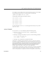
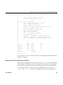
The module help command provides a list of all arguements accepted, as follows:
sys:~> module help
Modules Release 3.1.6 (Copyright GNU GPL v2 1991):
Available Commands and Usage:
+ add|load
modulefile [modulefile ...]
+ rm|unload
modulefile [modulefile ...]
+ switch|swap
modulefile1 modulefile2
+ display|show
modulefile [modulefile ...]
+ avail
[modulefile [modulefile ...]]
+ use [-a|--append]
dir [dir ...]
+ unuse
dir [dir ...]
+ update
+ purge
+ list
+ clear
+ help
[modulefile [modulefile ...]]
+ whatis
[modulefile [modulefile ...]]
+ apropos|keyword
string
+ initadd
modulefile [modulefile ...]
+ initprepend
modulefile [modulefile ...]
+ initrm
modulefile [modulefile ...]
+ initswitch
modulefile1 modulefile2
+ initlist
+ initclear
--------
For details about using modules, see the module(1) man page.
Library Overview
Libraries are files that contain one or more object (.o) files. Libraries are used to
simplify local software development by hiding compilation details. Libraries are
sometimes also called archives.
The SGI compiling environment contains several types of libraries; an overview about
each library is provided in this subsection.
007–5646–007
5
2: The SGI Compiling Environment
Static Libraries
Static libraries are used when calls to the library components are satisfied at link time
by copying text from the library into the executable. To create a static library, use the
ar(1), or an archiver command.
To use a static library, include the library name on the compiler’s command line. If
the library is not in a standard library directory, be sure to use the -L option to
specify the directory and the -l option to specify the library filename.
To build an appplication to have all static versions of standard libraries in the
application binary, use the -static option on the compiler command line.
Dynamic Libraries
Dynamic libraries are linked into the program at run time and when loaded into
memory can be accessed by multiple programs. Dynamic libraries are formed by
creating a Dynamic Shared Object (DSO).
Use the link editor command (ld(1)) to create a dynamic library from a series of
object files or to create a DSO from an existing static library.
To use a dynamic library, include the library on the compiler’s command line. If the
dynamic library is not in one of the standard library directories, use the -L path and
-l library_shortname compiler options during linking. You must also set the
LD_LIBRARY_PATH environment variable to the directory where the library is stored
before running the executable.
C/C++ Libraries
The following C/C++ libraries are provided with the Intel compiler:
• libguide.a, libguide.so: for support of OpenMP-based programs.
• libsvml.a: short vector math library
• libirc.a: Intel’s support for Profile-Guided Optimizations (PGO) and CPU
dispatch
• libimf.a, libimf.so: Intel’s math library
• libcprts.a, libcprts.so: Dinkumware C++ library
6
007–5646–007
®
®
Linux Application Tuning Guide for SGI X86-64 Based Systems
• libunwind.a, libunwind.so: Unwinder library
• libcxa.a, libcxa.so: Intel’s runtime support for C++ features
SHMEM Message Passing Libraries
The SHMEM application programing interface is implemented by the libsma library
and is part of the Message Passing Toolkit (MPT) product on SGI systems. The
SHMEM programming model consists of library routines that provide low-latency,
high-bandwidth communication for use in highly parallelized, scalable programs. The
routines in the SHMEM application programming interface (API) provide a
programming model for exchanging data between cooperating parallel processes. The
resulting programs are similar in style to Message Passing Interface (MPI) programs.
The SHMEM API can be used either alone or in combination with MPI routines in the
same parallel program.
A SHMEM program is SPMD (single program, multiple data) in style. The SHMEM
processes, called processing elements or PEs, all start at the same time, and they all
run the same program. Usually the PEs perform computation on their own
subdomains of the larger problem, and periodically communicate with other PEs to
exchange information on which the next computation phase depends.
The SHMEM routines minimize the overhead associated with data transfer requests,
maximize bandwidth, and minimize data latency. Data latency is the period of time
that starts when a PE initiates a transfer of data and ends when a PE can use the data.
SHMEM routines support remote data transfer through put operations, which transfer
data to a different PE, get operations, which transfer data from a different PE, and
remote pointers, which allow direct references to data objects owned by another PE.
Other operations supported are collective broadcast and reduction, barrier
synchronization, and atomic memory operations. An atomic memory operation is an
atomic read-and-update operation, such as a fetch-and-increment, on a remote or local
data object.
For details about using the SHMEM routines, see the intro_shmem(3) man page or
the Message Passing Toolkit (MPT) User’s Guide.
007–5646–007
7
Chapter 3
Performance Analysis and Debugging
Tuning an application involves determining the source of performance problems and
then rectifying those problems to make your programs run their fastest on the
available hardware. Performance gains usually fall into one of three categories of
measured time:
• User CPU time: time accumulated by a user process when it is attached to a CPU
and is executing.
• Elapsed (wall-clock) time: the amount of time that passes between the start and
the termination of a process.
• System time: the amount of time performing kernel functions like system calls,
sched_yield, for example, or floating point errors.
Any application tuning process involves the following steps:
1. Analyzing and identifying a problem
2. Locating where in the code the problem is
3. Applying an optimization technique
This chapter describes the process of analyzing your code to determine performance
bottlenecks. See Chapter 6, "Performance Tuning" on page 61, for details about tuning
your application for a single processor system and then tuning it for parallel
processing.
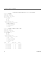
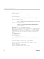
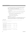
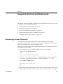
Determining System Configuration
One of the first steps in application tuning is to determine the details of the system
that you are running. Depending on your system configuration, different options
might or might not provide good results.
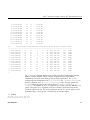
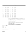
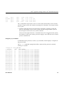
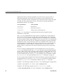
The topology(1) command displays general information about SGI systems, with a
focus on node information. This can include node counts for blades, node IDs,
NASIDs, memory per node, system serial number, partition number, UV Hub
versions, CPU to node mappings, and general CPU information. The topology
command is installed by the pcp-sgi RPM package.
007–5646–007
9
3: Performance Analysis and Debugging
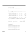
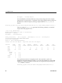
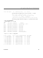
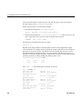
The following is example output from two topology(1) commands:
uv-sys:~ # topology
System type: UV2000
System name: harp34-sys
Serial number: UV2-00000034
Partition number: 0
8 Blades
256 CPUs
16 Nodes
235.82 GB Memory Total
15.00 GB Max Memory on any Node
1 BASE I/O Riser
2 Network Controllers
2 Storage Controllers
2 USB Controllers
1 VGA GPU
uv-sys:~ # topology --summary --nodes --cpus
System type: UV2000
System name: harp34-sys
Serial number: UV2-00000034
Partition number: 0
8 Blades
256 CPUs
16 Nodes
235.82 GB Memory Total
15.00 GB Max Memory on any Node
1 BASE I/O Riser
2 Network Controllers
2 Storage Controllers
2 USB Controllers
1 VGA GPU
Index
ID
NASID CPUS
Memory
-------------------------------------------0 r001i11b00h0
0
16
15316 MB
1 r001i11b00h1
2
16
15344 MB
2 r001i11b01h0
4
16
15344 MB
3 r001i11b01h1
6
16
15344 MB
4 r001i11b02h0
8
16
15344 MB
10
007–5646–007
®
®
Linux Application Tuning Guide for SGI X86-64 Based Systems
5
6
7
8
9
10
11
12
13
14
15
r001i11b02h1
r001i11b03h0
r001i11b03h1
r001i11b04h0
r001i11b04h1
r001i11b05h0
r001i11b05h1
r001i11b06h0
r001i11b06h1
r001i11b07h0
r001i11b07h1
10
12
14
16
18
20
22
24
26
28
30
16
16
16
16
16
16
16
16
16
16
16
15344
15344
15344
15344
15344
15344
15344
15344
15344
15344
15344
MB
MB
MB
MB
MB
MB
MB
MB
MB
MB
MB
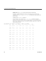
CPU
Blade PhysID CoreID APIC-ID Family Model Speed L1(KiB) L2(KiB) L3(KiB)
--------------------------------------------------------------------------------0 r001i11b00h0
00
00
0
6
45 2599 32d/32i
256
20480
1 r001i11b00h0
00
01
2
6
45 2599 32d/32i
256
20480
2 r001i11b00h0
00
02
4
6
45 2599 32d/32i
256
20480
3 r001i11b00h0
00
03
6
6
45 2599 32d/32i
256
20480
4 r001i11b00h0
00
04
8
6
45 2599 32d/32i
256
20480
5 r001i11b00h0
00
05
10
6
45 2599 32d/32i
256
20480
6 r001i11b00h0
00
06
12
6
45 2599 32d/32i
256
20480
7 r001i11b00h0
00
07
14
6
45 2599 32d/32i
256
20480
8 r001i11b00h1
01
00
32
6
45 2599 32d/32i
256
20480
9 r001i11b00h1
01
01
34
6
45 2599 32d/32i
256
20480
10 r001i11b00h1
01
02
36
6
45 2599 32d/32i
256
20480
11 r001i11b00h1
01
03
38
6
45 2599 32d/32i
256
20480
...
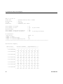
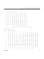
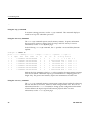
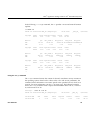
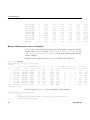
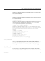
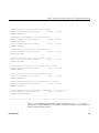
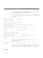
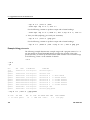
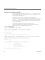
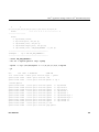
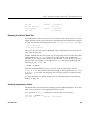
The cpumap(1) command displays logical CPUs and shows relationships between
them in a human-readable format. Aspects displayed include hyperthread
relationships, last level cache sharing, and topological placement. The cpumap
command gets its information from /proc/cpuinfo, the /sys/devices/system
directory structure, and /proc/sgi_uv/topology. When creating cpusets, the
Socket numbers reported in the output section Processor Numbering on
Socket(s) corresponds to the mems argument you would use in the definition of a
cpuset. The cpuset mems argument is the list of memory nodes that tasks in the
cpuset are allowed to use. For more information, see the SGI Cpuset Software Guide
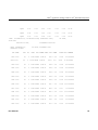
available at http://docs.sgi.com. The following is example output:
uv# cpumap
Thu Sep 19 10:17:21 CDT 2013
harp34-sys.americas.sgi.com
007–5646–007
11
3: Performance Analysis and Debugging
This is an SGI UV
model name
Architecture
cpu MHz
cache size
Total Number of
Total Number of
Hyperthreading
Total Number of
Total Number of
:
:
:
:
Genuine Intel(R) CPU @ 2.60GHz
x86_64
2599.946
20480 KB (Last Level)
Sockets
Cores
Physical Processors
Logical Processors
:
:
:
:
:
16
128
ON
128
256
(8 per socket)
(2 per Phys Processor)
UV Information
HUB Version:
UVHub 3.0
Number of Hubs:
16
Number of connected Hubs:
16
Number of connected NUMAlink ports:
128
=============================================================================
Hub-Processor Mapping
Hub Location
--- ---------0 r001i11b00h0
(
1 r001i11b00h1
(
2 r001i11b01h0
(
3 r001i11b01h1
(
4 r001i11b02h0
(
5 r001i11b02h1
(
6 r001i11b03h0
(
7 r001i11b03h1
(
12
Processor Numbers -- HyperThreads in ()
--------------------------------------0
1
2
3
4
5
6
7
128 129 130 131 132 133 134 135
8
9
10
11
12
13
14
15
136 137 138 139 140 141 142 143
16
17
18
19
20
21
22
23
144 145 146 147 148 149 150 151
24
25
26
27
28
29
30
31
152 153 154 155 156 157 158 159
32
33
34
35
36
37
38
39
160 161 162 163 164 165 166 167
40
41
42
43
44
45
46
47
168 169 170 171 172 173 174 175
48
49
50
51
52
53
54
55
176 177 178 179 180 181 182 183
56
57
58
59
60
61
62
63
184 185 186 187 188 189 190 191
)
)
)
)
)
)
)
)
007–5646–007
®
®
Linux Application Tuning Guide for SGI X86-64 Based Systems
8 r001i11b04h0
(
9 r001i11b04h1
(
10 r001i11b05h0
(
11 r001i11b05h1
(
12 r001i11b06h0
(
13 r001i11b06h1
(
14 r001i11b07h0
(
15 r001i11b07h1
(
64
192
72
200
80
208
88
216
96
224
104
232
112
240
120
248
65
193
73
201
81
209
89
217
97
225
105
233
113
241
121
249
66
194
74
202
82
210
90
218
98
226
106
234
114
242
122
250
67
195
75
203
83
211
91
219
99
227
107
235
115
243
123
251
68
196
76
204
84
212
92
220
100
228
108
236
116
244
124
252
69
197
77
205
85
213
93
221
101
229
109
237
117
245
125
253
70
198
78
206
86
214
94
222
102
230
110
238
118
246
126
254
71
199
79
207
87
215
95
223
103
231
111
239
119
247
127
255
)
)
)
)
)
)
)
)
=============================================================================
Processor Numbering on Node(s)
Node
-----0
1
2
3
4
5
6
7
8
9
10
11
12
13
14
15
(Logical) Processors
------------------------0
1
2
3
4
5
8
9
10
11
12
13
16
17
18
19
20
21
24
25
26
27
28
29
32
33
34
35
36
37
40
41
42
43
44
45
48
49
50
51
52
53
56
57
58
59
60
61
64
65
66
67
68
69
72
73
74
75
76
77
80
81
82
83
84
85
88
89
90
91
92
93
96
97
98
99 100 101
104 105 106 107 108 109
112 113 114 115 116 117
120 121 122 123 124 125
6
14
22
30
38
46
54
62
70
78
86
94
102
110
118
126
7
15
23
31
39
47
55
63
71
79
87
95
103
111
119
127
128
136
144
152
160
168
176
184
192
200
208
216
224
232
240
248
129
137
145
153
161
169
177
185
193
201
209
217
225
233
241
249
130
138
146
154
162
170
178
186
194
202
210
218
226
234
242
250
131
139
147
155
163
171
179
187
195
203
211
219
227
235
243
251
132
140
148
156
164
172
180
188
196
204
212
220
228
236
244
252
133
141
149
157
165
173
181
189
197
205
213
221
229
237
245
253
134
142
150
158
166
174
182
190
198
206
214
222
230
238
246
254
135
143
151
159
167
175
183
191
199
207
215
223
231
239
247
255
=============================================================================
007–5646–007
13
3: Performance Analysis and Debugging
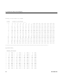
Sharing of Last Level (3) Caches
Socket
-----0
1
2
3
4
5
6
7
8
9
10
11
12
13
14
15
(Logical) Processors
------------------------0
1
2
3
4
5
8
9
10
11
12
13
16
17
18
19
20
21
24
25
26
27
28
29
32
33
34
35
36
37
40
41
42
43
44
45
48
49
50
51
52
53
56
57
58
59
60
61
64
65
66
67
68
69
72
73
74
75
76
77
80
81
82
83
84
85
88
89
90
91
92
93
96
97
98
99 100 101
104 105 106 107 108 109
112 113 114 115 116 117
120 121 122 123 124 125
6
14
22
30
38
46
54
62
70
78
86
94
102
110
118
126
7
15
23
31
39
47
55
63
71
79
87
95
103
111
119
127
128
136
144
152
160
168
176
184
192
200
208
216
224
232
240
248
129
137
145
153
161
169
177
185
193
201
209
217
225
233
241
249
130
138
146
154
162
170
178
186
194
202
210
218
226
234
242
250
131
139
147
155
163
171
179
187
195
203
211
219
227
235
243
251
132
140
148
156
164
172
180
188
196
204
212
220
228
236
244
252
133
141
149
157
165
173
181
189
197
205
213
221
229
237
245
253
134
142
150
158
166
174
182
190
198
206
214
222
230
238
246
254
135
143
151
159
167
175
183
191
199
207
215
223
231
239
247
255
=============================================================================
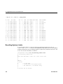
HyperThreading
Shared Processors
----------------(
0, 128) (
1,
(
4, 132) (
5,
(
8, 136) (
9,
(
12, 140) (
13,
(
16, 144) (
17,
(
20, 148) (
21,
(
24, 152) (
25,
(
28, 156) (
29,
(
32, 160) (
33,
(
36, 164) (
37,
(
40, 168) (
41,
(
44, 172) (
45,
(
48, 176) (
49,
14
129)
133)
137)
141)
145)
149)
153)
157)
161)
165)
169)
173)
177)
(
(
(
(
(
(
(
(
(
(
(
(
(
2,
6,
10,
14,
18,
22,
26,
30,
34,
38,
42,
46,
50,
130)
134)
138)
142)
146)
150)
154)
158)
162)
166)
170)
174)
178)
(
(
(
(
(
(
(
(
(
(
(
(
(
3,
7,
11,
15,
19,
23,
27,
31,
35,
39,
43,
47,
51,
131)
135)
139)
143)
147)
151)
155)
159)
163)
167)
171)
175)
179)
007–5646–007
®
®
Linux Application Tuning Guide for SGI X86-64 Based Systems
(
(
(
(
(
(
(
(
(
(
(
(
(
(
(
(
(
(
(
52,
56,
60,
64,
68,
72,
76,
80,
84,
88,
92,
96,
100,
104,
108,
112,
116,
120,
124,
180)
184)
188)
192)
196)
200)
204)
208)
212)
216)
220)
224)
228)
232)
236)
240)
244)
248)
252)
(
(
(
(
(
(
(
(
(
(
(
(
(
(
(
(
(
(
(
53,
57,
61,
65,
69,
73,
77,
81,
85,
89,
93,
97,
101,
105,
109,
113,
117,
121,
125,
181)
185)
189)
193)
197)
201)
205)
209)
213)
217)
221)
225)
229)
233)
237)
241)
245)
249)
253)
(
(
(
(
(
(
(
(
(
(
(
(
(
(
(
(
(
(
(
54,
58,
62,
66,
70,
74,
78,
82,
86,
90,
94,
98,
102,
106,
110,
114,
118,
122,
126,
182)
186)
190)
194)
198)
202)
206)
210)
214)
218)
222)
226)
230)
234)
238)
242)
246)
250)
254)
(
(
(
(
(
(
(
(
(
(
(
(
(
(
(
(
(
(
(
55,
59,
63,
67,
71,
75,
79,
83,
87,
91,
95,
99,
103,
107,
111,
115,
119,
123,
127,
183)
187)
191)
195)
199)
203)
207)
211)
215)
219)
223)
227)
231)
235)
239)
243)
247)
251)
255)
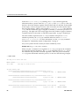
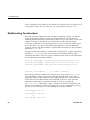
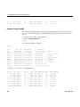
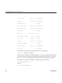
The x86info(1) command displays x86 CPU diagnostics information. Type one of
the following commands to load the x86info(1) command if the command is not
already installed:
• On Red Hat Enterprise Linux (RHEL) systems, type the following:
# yum install x86info.x86_64
• On SUSE Linux Enterprise Server (SLES) systems, type the following:
# zypper install x86info
The following is an example of x86info(1) command output:
uv44-sys:~ # x86info
x86info v1.25. Dave Jones 2001-2009
Feedback to .
Found 64 CPUs
-------------------------------------------------------------------------CPU #1
EFamily: 0 EModel: 2 Family: 6 Model: 46 Stepping: 6
CPU Model: Unknown model.
007–5646–007
15
3: Performance Analysis and Debugging
Processor name string: Intel(R) Xeon(R) CPU
E7520 @ 1.87GHz
Type: 0 (Original OEM) Brand: 0 (Unsupported)
Number of cores per physical package=16
Number of logical processors per socket=32
Number of logical processors per core=2
APIC ID: 0x0
Package: 0 Core: 0
SMT ID 0
-------------------------------------------------------------------------CPU #2
EFamily: 0 EModel: 2 Family: 6 Model: 46 Stepping: 6
CPU Model: Unknown model.
Processor name string: Intel(R) Xeon(R) CPU
E7520 @ 1.87GHz
Type: 0 (Original OEM) Brand: 0 (Unsupported)
Number of cores per physical package=16
Number of logical processors per socket=32
Number of logical processors per core=2
APIC ID: 0x6
Package: 0 Core: 0
SMT ID 6
-------------------------------------------------------------------------CPU #3
EFamily: 0 EModel: 2 Family: 6 Model: 46 Stepping: 6
CPU Model: Unknown model.
Processor name string: Intel(R) Xeon(R) CPU
E7520 @ 1.87GHz
Type: 0 (Original OEM) Brand: 0 (Unsupported)
Number of cores per physical package=16
Number of logical processors per socket=32
Number of logical processors per core=2
APIC ID: 0x10
Package: 0 Core: 0
SMT ID 16
-------------------------------------------------------------------------...
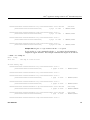
You can also use the uname command, which returns the kernel version and other
machine information. For example:
uv44-sys:~ # uname -a
Linux uv44-sys 2.6.32.13-0.4.1.1559.0.PTF-default #1 SMP 2010-06-15 12:47:25 +0200 x86_64 x86_64 x86_64
For more system information, change directory to the
/sys/devices/system/node/node0/cpu0/cache directory and list the contents.
For example:
uv44-sys:/sys/devices/system/node/node0/cpu0/cache # ls
index0 index1 index2 index3
16
007–5646–007
®
®
Linux Application Tuning Guide for SGI X86-64 Based Systems
Change directory to index0 and list the contents, as follows:
uv44-sys:/sys/devices/system/node/node0/cpu0/cache/index0 # ls
coherency_line_size level number_of_sets physical_line_partition
shared_cpu_list
shared_cpu_map
size
Sources of Performance Problems
There are usually three areas of program execution that can have performance
slowdowns:
• CPU-bound processes: processes that are performing slow operations (such as
sqrt or floating-point divides) or non-pipelined operations such as switching
between add and multiply operations.
• Memory-bound processes: code which uses poor memory strides, occurrences of
page thrashing or cache misses, or poor data placement in NUMA systems.
• I/O-bound processes: processes which are waiting on synchronous I/O, formatted
I/O, or when there is library or system level buffering.
Several profiling tools can help pinpoint where performance slowdowns are
occurring. The following sections describe some of these tools.
Profiling with perf
Linux Performance Events provides a performance analysis framework for systems
that use Intel Xeon Phi technology. It includes hardware-level CPU performance
monitoring unit (PMU) features, software counters, and tracepoints.
Before you use these profiling tools, make sure the perf RPM is installed. The perf
RPM comes with the your operating system and is not an SGI product.
For more information, see the following man pages: perf(1), perf-stat(1),
perf-top(1), perf-record(1), perf-report(1), perf-list(1). The perf RPM
includes these man pages.
Profiling with PerfSuite
PerfSuite is a set of tools, utilities, and libraries that you can use to analyze
application software performance Linux-based systems. You can use PerfSuite tools to
007–5646–007
17
type
way
3: Performance Analysis and Debugging
perform performance-related activities, ranging from assistance with compiler
optimization reports to hardware performance counting, profiling, and MPI usage
summarization. PerfSuite is Open Source software. It is approved for licensing under
the University of Illinois/NCSA Open Source License (OSI-approved).
For more information, see one of the following websites:
• http://perfsuite.ncsa.uiuc.edu/
• http://perfsuite.sourceforge.net/
• http://www.ncsa.illinois.edu/UserInfo/Resources/Software/Tools/PerfSuite/,
which hosts NCSA-specific information about using PerfSuite tools
The psrun utility is a PerfSuite command line utility that gathers hardware
performance information on an unmodified executable. For more information, see
http://perfsuite.ncsa.uiuc.edu/psrun/.
Other Performance Analysis Tools
The following tools might be useful to you when you try to optimize your code:
• The Intel® VTuneTM Amplifier XE, which is a performance and thread profiler. This
tool does remote sampling experiments. The VTune data collector runs on the
Linux system and an accompanying GUI runs on an IA-32 Windows machine,
which is used for analyzing the results. VTune allows you to perform interactive
experiments while connected to the host through its GUI. An additional tool, the
Performance Tuning Utility (PTU), requires the Intel VTune license.
For information about Intel VTune Amplifier XE, see the following URL:
http://software.intel.com/en-us/intel-vtune-amplifier-xe#pid-3773–760
• Intel Inspector XE, which is a memory and thread debugger. For information
about Intel Inspector XE, see the following:
http://software.intel.com/en-us/intel-inspector-xe/
• Intel Advisor XE, which is a threading design and prototyping tool. For
information about Intel Advisor XE, see the following:
http://software.intel.com/en-us/intel-advisor-xe
18
007–5646–007
®
®
Linux Application Tuning Guide for SGI X86-64 Based Systems
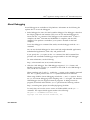
About Debugging
Several debuggers are available on SGI platforms. Information in the following list
explains how to access the debuggers:
• Intel® Debugger for Linux, the Intel symbolic debugger. This debugger is based on
the Eclipse graphical user interface (GUI). You can run the Intel Debugger for
Linux from the idb command. This debugger works with the Intel® C and C++
compilers, the Intel® Fortran90 and FORTRAN 77 compilers, and the GNU
compilers. This product is available if your system is licensed for the Intel
compilers.
To run the debugger in command line mode, start the debugger with the idbc
command.
You can use the Intel Debugger for Linux with both single-threaded applications,
multithreaded applications, serial code, and parallel code.
If you specify the -gdb option on the idb command, the shell command line
provides user commands and debugger output similar to the GNU debugger.
For more information, see the following:
http://software.intel.com/en-us/articles/idb-linux/
• GDB, the GNU debugger. The GDB debugger supports C, C++, Fortran, and
Modula-2 programs. Use the gdb command to start GDB. To use GDB through a
GUI, use the ddd command.
When compiling with C and C++, include the -g option on the compiler command
line. The -g option produces the dwarf2 symbols database that GDB uses.
When using GDB for Fortran debugging, include the -g and -O0 options. Do not
use gdb for Fortran debugging when compiling with -O1 or higher. The standard
GDB debugger does not support Fortran 95 programs. To debug Fortran 95
programs, download and install the gdbf95 patch from the following website:
http://sourceforge.net/project/showfiles.php?group_id=56720
To verify that you have the correct version of GDB installed, use the gdb -v
command. The output should appear similar to the following:
GNU gdb 5.1.1 FORTRAN95-20020628 (RC1)
Copyright 2012 Free Software Foundation, Inc.
007–5646–007
19
3: Performance Analysis and Debugging
For a complete list of GDB commands, use the help option or see the following
user guide:
http://sources.redhat.com/gdb/onlinedocs/gdb_toc.html
Note that the current instances of GDB do not report ar.ec registers correctly. If
you are debugging rotating, register-based, software-pipelined loops at the
assembly code level, try using the Intel Debugger for Linux.
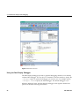
• TotalView, which is a licensed graphical debugger that you can use with MPI
programs. For information about TotalView, see the following:
http://www.roguewave.com
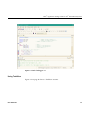
In addition to the preceding debuggers, you can start the Intel Debugger and GDB
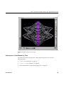
with the ddd command. The ddd command starts the Data Display Debugger, a GNU
product that provides a graphical debugging interface.
The following topics provide more information:
• "Using the Intel Debugger" on page 20
• "Using TotalView" on page 21
• "Using the Data Display Debugger" on page 22
Using the Intel Debugger
The Intel Debugger idb is part of Intel® Composer XE. You are asked during the
installation if you want to install it or not. The idb command starts the graphical
user interface (GUI). The idbc command starts the command line interface.
The following figure shows the GUI:
20
007–5646–007
®
®
Linux Application Tuning Guide for SGI X86-64 Based Systems
Figure 3-1 Intel® Debugger GUI
Using TotalView
Figure 3-2 on page 22 shows a TotalView sesssion.
007–5646–007
21
3: Performance Analysis and Debugging
Figure 3-2 TotalView Session
Using the Data Display Debugger
The Data Display Debugger provides a graphical debugging interface to an arbitrary
command line debugger. You use the ddd command to start this interface. Specify the
--debugger option to specify the debugger you want to use. For example, specify
--debugger "idb" to specify the Intel Debugger. The default debugger is gdb.
When the debugger loads, the Data Display Debugger screen appears divided into
panes that show the following information:
22
007–5646–007
®
®
Linux Application Tuning Guide for SGI X86-64 Based Systems
• Array inspection
• Source code
• Disassembled code
• A command line window to the debugger engine
These panes can be switched on and off from the View menu.
Some commonly used commands can be found on the menus. In addition, the
following actions can be useful:
• Select an address in the assembly view, click the right mouse button, and select
lookup. The gdb command is executed in the command pane and it shows the
corresponding source line.
• Select a variable in the source pane and click the right mouse button. The current
value is displayed. Arrays are displayed in the array inspection window. You can
print these arrays to PostScript by using the Menu>Print Graph option.
• You can view the contents of the register file, including general, floating-point,
NaT, predicate, and application registers by selecting Registers from the Status
menu. The Status menu also allows you to view stack traces or to switch OpenMP
threads.
007–5646–007
23
Chapter 4
Monitoring Tools
This chapter describes several tools that you can use to monitor system performance.
The tools are divided into two general categories: system monitoring tools and
nonuniform memory access (NUMA) tools.
System monitoring tools include the topology(1), top(1) commands and the
Performance Co-Pilot pmchart(1) commmand and other operating system commands
such as the vmstat(1) , iostat(1) command and the sar(1) commands that can help
you determine where system resources are being spent.
The gtopology(1) command displays a 3D scene of the system interconnect using
the output from the topology(1) command.
System Monitoring Tools
You can use system utilities to better understand the usage and limits of your system.
These utilities allow you to observe both overall system performance and
single-performance execution characteristics. This section covers the following topics:
• "Hardware Inventory and Usage Commands" on page 25
• "Performance Co-Pilot Monitoring Tools" on page 29
• "System Usage Commands" on page 32
• "Memory Statistics and nodeinfo Command" on page 36
Hardware Inventory and Usage Commands
This section descibes hardware inventory and usage commands and covers the
following topics:
• "topology(1) Command" on page 25
• "gtopology(1) Command" on page 26
topology(1) Command
The topology(1) command provides topology information about your system.
007–5646–007
25
4: Monitoring Tools
Applications programmers can use the topology command to help optimize
execution layout for their applications. For more information, see the topology(1)
man page.
For an example of the topology command’s output, see "Determining System
Configuration" on page 9.
gtopology(1) Command
The gtopology(1) command is included as part of the sgi-pcp package of the SGI
Accelerate, part of SGI Performance Suite software. It displays a 3D scene of the
system interconnect using the output from the topology(1) command. See the man
page for more details.
Figure 4-1 on page 27, shows the ring topology (the eight nodes are shown in pink,
the NUMAlink connections in cyan) of an SGI system with 16 CPUs.
26
007–5646–007
®
®
Linux Application Tuning Guide for SGI X86-64 Based Systems
Figure 4-1 Ring Topology of an System with 16 CPUs
Figure 4-2 on page 28, shows the fat-tree topology of an SGI system with 32 CPUs.
Again, nodes are the pink cubes. Routers are shown as blue spheres (if all ports are
used) otherwise, yellow.
007–5646–007
27
4: Monitoring Tools
Figure 4-2 An SGI System with 32 CPUs Fat-tree Topology
Figure 4-3 on page 29, shows an SGI system with 512 CPUs. The dual planes of the
fat-tree topology are clearly visible.
28
007–5646–007
®
®
Linux Application Tuning Guide for SGI X86-64 Based Systems
Figure 4-3 An SGI System with 512 CPUs
Performance Co-Pilot Monitoring Tools
This section describes Performance Co-Pilot monitoring tools and covers the
following topics:
• "hubstats(1) Command" on page 30
• "linkstat-uv(1) Command" on page 30
• "Other Performance Co-Pilot Monitoring Tools" on page 30
007–5646–007
29
4: Monitoring Tools
hubstats(1) Command
The hubstats(1) command monitors NUMAlink traffic, directory cache operations,
and global reference unit (GRU) traffic statistics on SGI UV systems. It does not work
on any other platform. For more information, see the hubstats(1) man page.
linkstat-uv(1) Command
The linkstat-uv(1) command monitors NUMAlink traffic and error rates on SGI
UV systems. It does not work on any other platform. This command returns
information about packets and Mbytes sent/received on each NUMAlink in the
system, as well as error rates. It is useful as a performance monitoring tool and as a
tool for helping you to diagnose and identify faulty hardware. For more information,
see the linkstat-uv(1) man page.
Note that this command is specific to SGI UV systems and does not return the same
information as the linkstat(1) command.
Other Performance Co-Pilot Monitoring Tools
In addition to the UV specific tools described above, the pcp and pcp-sgi packages
also provide numerous other performance monitoring tools, both graphical and
text-based. It is important to remember that all of the performance metrics displayed
by any of the tools described in this chapter can also be monitored with other tools
such as pmchart(1), pmval(1), pminfo(1) and others. Additionally, the pmlogger(1)
command can be used to capture Performance Co-Pilot archives, which can then be
"replayed" during a retrospective performance analysis.
A very brief description of other Performance Co-Pilot monitoring tools follows. See
the associated man page for each tool for more details.
• pmchart(1) — graphical stripchart tool, chiefly used for investigative performance
analysis.
• pmgsys(1) — graphical tool showing miniature CPU, Disk, Network, LoadAvg
and memory/swap in a miniature display, for example, useful for permanent
residence on your desktop for the servers you care about.
• pmgcluster(1) — pmgsys, but for multiple hosts and thus useful for monitoring
a cluster of hosts or servers.
• clustervis(1) – 3D display showing per-CPU and per-Network performance for
multiple hosts.
30
007–5646–007
®
®
Linux Application Tuning Guide for SGI X86-64 Based Systems
• nfsvis(1) – 3D display showing NFS client/server traffic, grouped by NFS
operation type
• nodevis(1) – 3D display showing per-node CPU and memory usage.
• webvis(1) – 3D display showing per-httpd traffic.
• dkvis(1) - 3D display showing per-disk traffic, grouped by controller.
• diskstat(1) – command line tool for monitoring disk traffic.
• topdisk(1) – command line, curses-based tool, for monitoring disk traffic.
• topsys(1) – command line, curses-based tool, for monitoring processes making a
large numbers of system calls or spending a large percentage of their execution
time in system mode using assorted system time measures.
• pmgxvm(1) – miniature graphical display showing XVM volume topology and
performance statistics.
• osvis(1) – 3D display showing assorted kernel and system statistics.
• pmdumptext(1) — command line tool for monitoring multiple performance
metrics with a highly configurable output format. Therefore, it is a useful tools for
scripted monitoring tasks.
• pmval(1) — command line tool, similar to pmdumptext(1), but less flexible.
• pminfo(1) — command line tool, useful for printing raw performance metric
values and associated help text.
• pmprobe(1) — command line tool useful for scripted monitoring tasks.
• pmie(1) — a performance monitoring inference engine. This is a command line
tool with an extraordinarily powerful underlying language. It can also be used as
a system service for monitoring and reporting on all sorts of performance issues of
interest.
• pmieconf(1) - command line tool for creating and customizing "canned" pmie(1)
configurations.
• pmlogger(1) – command line tool for capturing Performance Co-Pilot
performance metrics archives for replay with other tools.
• pmlogger_daily(1) and pmlogger_check(1) – cron driven infrastructure for
automated logging with pmlogger(1).
007–5646–007
31
4: Monitoring Tools
• pmcd(1) – the Performance Co-Pilot metrics collector daemon
• PCPIntro(1) - introduction to Performance Co-Pilot monitoring tools, generic
command line usage and environment variables
• PMAPI(3) - introduction to the Performance Co-Pilot API libraries for developing
new performance monitoring tools
• PMDA(3) - introduction to the Performance Co-Pilot Metrics Domain Agent API, for
developing new Performance Co-Pilot agents
• topology(1) – displays general information about SGI UV systems, with a focus
on node information. This includes counts of the CPUs, nodes, routers and
memory, as well as, various I/O devices. More detailed information is available
for node IDs, NASIDs, memory per node, system serial number, partition number,
UV Hub versions, CPU to node mappings, I/O device descriptions, and general
CPU and I/O information.
System Usage Commands
The following topics show several commands that can be used to determine user
load, system usage, and active processes:
• "Using the w command" on page 32
• "Using the ps(1) Command" on page 33
• "Using the top(1) Command" on page 34
• "Using the vmstat(8) Command" on page 34
• "Using the iostat(1) command" on page 34
• "Using the sar(1) command" on page 35
Using the w command
To obtain a high-level view of system usage that includes information about who is
logged into the system, use the w(1) command, as follows:
uv44-sys:~ # w
15:47:48 up 2:49, 5 users, load average: 0.04, 0.27, 0.42
USER
TTY
LOGIN@
IDLE
JCPU
PCPU WHAT
root
pts/0
13:10
1:41m 0.07s 0.07s -bash
32
007–5646–007
®
®
Linux Application Tuning Guide for SGI X86-64 Based Systems
root
boetcher
root
root
pts/2
pts/4
pts/5
pts/6
13:31
14:30
14:32
15:09
0.00s
2:13
1:14m
31:25
0.14s
0.73s
0.04s
0.08s
0.02s
0.73s
0.04s
0.08s
w
-csh
-bash
-bash
The w command’s output shows who is on the system, the duration of user sessions,
processor usage by user, and currently executing user commands. The output consists
of two parts:
• The first output line shows the current time, the length of time the system has
been up, the number of users on the system, and the average number of jobs in
the run queue in the last one, five, and 15 minutes.
The rest of the output from the w command shows who is logged into the system,
the duration of each user session, processor usage by user, and each user’s current
process command line.
Using the ps(1) Command
To determine active processes, use the ps(1) command, which displays a snapshot of
the process table.
The ps -A r command example that follows returns all the processes currently
running on a system:
[user@profit user]# ps
PID TTY
STAT
211116 pts/0
R+
211117 pts/0
R+
211118 pts/0
R+
211119 pts/0
R+
211120 pts/0
R+
211121 pts/0
R+
211122 pts/0
R+
211123 pts/0
R+
211124 pts/0
R+
211125 pts/0
R+
211126 pts/0
R+
211127 pts/0
R+
211128 pts/0
R+
211129 pts/0
R+
211130 pts/0
R+
211131 pts/0
R+
007–5646–007
-A r
TIME
4:08
4:08
4:08
4:08
4:08
4:08
4:08
4:08
4:08
4:08
4:08
4:08
4:08
4:08
4:08
4:08
COMMAND
/usr/diags/bin/olconft
/usr/diags/bin/olconft
/usr/diags/bin/olconft
/usr/diags/bin/olconft
/usr/diags/bin/olconft
/usr/diags/bin/olconft
/usr/diags/bin/olconft
/usr/diags/bin/olconft
/usr/diags/bin/olconft
/usr/diags/bin/olconft
/usr/diags/bin/olconft
/usr/diags/bin/olconft
/usr/diags/bin/olconft
/usr/diags/bin/olconft
/usr/diags/bin/olconft
/usr/diags/bin/olconft
RUNTIME=5
RUNTIME=5
RUNTIME=5
RUNTIME=5
RUNTIME=5
RUNTIME=5
RUNTIME=5
RUNTIME=5
RUNTIME=5
RUNTIME=5
RUNTIME=5
RUNTIME=5
RUNTIME=5
RUNTIME=5
RUNTIME=5
RUNTIME=5
33
4: Monitoring Tools
...
Using the top(1) Command
To monitor running processes, use the top(1) command. This command displays a
sorted list of top CPU utilization processes.
Using the vmstat(8) Command
The vmstat(8) command reports virtual memory statistics. It reports information
about processes, memory, paging, block IO, traps, and CPU activity. For more
information, see the vmstat(8) man page.
In the following vmstat(8) command, the 10 specifies a 10–second delay between
updates.
uv44-sys:~ # vmstat 10
procs -----------memory---------- ---swap-- -----io---- --system-- -----cpu----r b
swpd
free
buff cache
si
so
bi
bo
in
cs us sy id wa st
2 0
0 235984032 418748 8649568
0
0
0
0
0
0 0 0 100 0
1 0
0 236054400 418748 8645216
0
0
0 4809 256729 3401 0 0 100
1 0
0 236188016 418748 8649904
0
0
0
448 256200 631 0 0 100
2 0
0 236202976 418748 8645104
0
0
0
341 256201 1117 0 0 100
1 0
0 236088720 418748 8592616
0
0
0
847 257104 6152 0 0 100
1 0
0 235990944 418748 8648460
0
0
0
240 257085 5960 0 0 100
1 0
0 236049568 418748 8645100
0
0
0 4849 256749 3604 0 0 100
0
0
0
0
0
0
0
0
0
0
0
0
0
Without the delay parameter, which is 10 in this example, the output returns averages
since the last reboot. Additional reports give information on a sampling period of
length delay. The process and memory reports are instantaneous in either case.
Using the iostat(1) command
The iostat(1) command monitors system input/output device loading by observing
the time the devices are active, relative to their average transfer rates. You can use
information from the iostat command to change system configuration information
to better balance the input/output load between physical disks. For more
information, see the iostat(1) man page.
34
007–5646–007
®
®
Linux Application Tuning Guide for SGI X86-64 Based Systems
In the following iostat(1) command, the 10 specifies a 10–second interval between
updates:
# iostat 10
Linux 2.6.32-430.el6.x86_64 (harp34-sys)
avg-cpu:
%user
46.24
Device:
sda
sdb
avg-cpu:
tps
53.66
0.01
%user
99.96
Device:
sda
sdb
avg-cpu:
%nice %system %iowait
0.01
0.67
0.01
Device:
sda
sdb
...
Blk_read/s
149312.00
0.00
Blk_read/s
146746.05
0.00
%steal
0.00
Blk_wrtn/s
150423.20
0.00
%nice %system %iowait
0.00
0.05
0.00
tps
305.19
0.00
%steal
0.00
_x86_64_
(256 CPU)
%idle
53.08
Blk_wrtn/s
Blk_read
Blk_wrtn
23791.93 21795308343 21869098736
0.00
17795
0
%nice %system %iowait
0.00
0.04
0.00
tps
321.20
0.00
%user
99.95
Blk_read/s
23711.65
0.02
02/21/2014
%steal
0.00
Blk_wrtn/s
148453.95
0.00
%idle
0.00
Blk_read
1493120
0
Blk_wrtn
1504232
0
%idle
0.00
Blk_read
1468928
0
Blk_wrtn
1486024
0
Using the sar(1) command
The sar(1) command returns the content of selected, cumulative activity counters in
the operating system. Based on the values in the count and interval parameters, the
command writes information count times spaced at the specified interval, which is in
seconds. For more information, see the sar(1) man page. The following example
shows the sar(1) command with a request for information about CPU 1, a count of
10, and an interval of 10:
uv44-sys:~ # sar -P 1 10 10
Linux 2.6.32-416.el6.x86_64 (harp34-sys)
11:24:54 AM
11:25:04 AM
007–5646–007
CPU
1
%user
0.20
%nice
0.00
09/19/2013
%system
0.10
%iowait
0.00
_x86_64_
(256 CPU)
%steal
0.00
%idle
99.70
35
4: Monitoring Tools
11:25:14
11:25:24
11:25:34
11:25:44
11:25:54
11:26:04
11:26:14
11:26:24
11:26:34
Average:
AM
AM
AM
AM
AM
AM
AM
AM
AM
1
1
1
1
1
1
1
1
1
1
10.10
99.70
99.70
8.99
0.10
38.70
99.80
80.42
0.10
43.78
0.00
0.00
0.00
0.00
0.00
0.00
0.00
0.00
0.00
0.00
0.30
0.30
0.30
0.60
0.20
0.10
0.10
0.70
0.20
0.29
0.00
0.00
0.00
0.00
0.00
0.00
0.00
0.00
0.00
0.00
0.00
0.00
0.00
0.00
0.00
0.00
0.00
0.00
0.00
0.00
89.60
0.00
0.00
90.41
99.70
61.20
0.10
18.88
99.70
55.93
Memory Statistics and nodeinfo Command
nodeinfo(1) is a tool for monitoring per-node NUMA memory statistics on SGI UV
systems. The nodeinfo tool reads /sys/devices/system/node/*/meminfo and
/sys/devices/system/node/*/numastat on the local system to gather NUMA
memory statistics.
Sample memory statistic from the nodeinfo(1) command are, as follows:
uv44-sys:~ # nodeinfo
Memory Statistics Tue Oct 26 12:01:58 2010
uv44-sys
---------------------- Per Node KB ------------------------
------ Preferred Alloc ------miss foreign interlv
-- Loc/Rem ---
node
Total
Free
Used
Dirty
Anon
Slab
hit
local
remote
0
1
16757488
16777216
16277084
16433988
480404
343228
52
68
34284
6772
36288
17708
20724
4477
0
0
0
0
0
0
20720
3381
4
1096
2
16777216
16438568
338648
76
6908
12620
1804
0
0
0
709
1095
3
16760832
16429844
330988
56
2820
16836
1802
0
0
0
708
1094
4
16777216
16444408
332808
88
10124
13588
1517
0
0
0
417
1100
5
16760832
16430300
330532
72
1956
17304
4546
0
0
0
3453
1093
6
7
16777216
16760832
16430788
16435532
346428
325300
36
44
3236
1220
15292
14800
3961
3971
0
0
0
0
0
0
2864
2877
1097
1094
TOT
134148848
131320512
2828336
492
67320
144436
42802
0
0
0
35129
7673
Press "h" for help
From an interactive nodeinfo session, enter h for a help statement:
Display memory statistics by node.
q
quit
+
Increase starting node number. Used only if more nodes than will
fit in the current window.
36
007–5646–007
®
®
Linux Application Tuning Guide for SGI X86-64 Based Systems
b
e
k
m
p
t
A
H
L
Decrease starting node number. Used only if more nodes than will
fit in the current window.
Start output with node 0.
Show highest node number.
show sizes in KB.
show sizes in MB.
show sizes in pages.
Change refresh rate.
Show/Hide memory policy stats.
Show/Hide hugepage info.
Show/Hide LRU Queue stats.
Field definitions:
hit - page was allocated on the preferred node
miss - preferred node was full. Allocation occurred on THIS node
by a process running on another node that was full
foreign - Preferred node was full. Had to allocate somewhere
else.
interlv - allocation was for interleaved policy
local - page allocated on THIS node by a process running on THIS node
remote - page allocated on THIS node by a process running on ANOTHER node
(press any key to exit from help screen)
007–5646–007
37
Chapter 5
Data Process and Placement Tools
This chapter contains the following topics:
• "About Nonuniform Memory Access (NUMA) Computers" on page 39
• "About the Data and Process Placement Tools" on page 41
About Nonuniform Memory Access (NUMA) Computers
On symmetric multiprocessor (SMP) computers, all data is visible from all processors.
Each processor is functionally identical and has equal time access to every memory
address. That is, all processors have equally fast (symmetric) access to memory. These
types of systems are easy to assemble and have limited scalability due to memory
access times.
NUMA computers also have a shared address space. In both cases, there is a single
shared memory space and a single operating system instance. However, in an SMP
computer, each processor is functionally identical and has equal time access to every
memory address.
In contrast, a NUMA system has a shared address space, but the access time to
memory varies over physical address ranges and between processing elements. The
Intel Xeon 7500 series processor (i7 architecture) is an example of NUMA architecture.
Each processor has its own memory and can address the memory attached to another
processor through the Quick Path Interconnect (QPI).
The SGI UV 1000 series is a family of multiprocessor, distributed shared memory
(DSM) computer systems that initially scale from 32 to 2560 Intel processor cores, as a
cache-coherent single system image (SSI). The SGI UV 100 series is a family of
multiprocessor distributed shared memory (DSM) computer systems that initially
scale from 16 to 768 Intel processor cores as a cache-coherent SSI. The SGI UV 2000
series scales from 32 to 4,096 Intel processor cores as a cache-coherent SSI.
There are two levels of NUMA: intranode, managed by the Intel QPI, and internode,
managed through the SGI HUB ASIC and SGI NUMAlink 5 or SGI NUMAlink 6.
The following topics explain other aspects of the SGI NUMA computers:
• "Distributed Shared Memory (DSM)" on page 40
007–5646–007
39
5: Data Process and Placement Tools
• "ccNUMA Architecture" on page 40
Distributed Shared Memory (DSM)
Scalability is the measure of how the work done on a computing system changes as
you add CPUs, memory, network bandwidth, I/O capacity, and other resources.
Many factors, for example, memory latency across the system, can affect scalability.
In the SGI UV 2000, SGI UV 1000, and SGI UV 100 series systems, memory is
physically distributed both within and among the IRU enclosures, which consist of
the compute, memory, and I/O blades. However, memory is accessible to and shared
by all devices, connected by NUMAlink, within the single-system image (SSI). In
other words, all components connected by NUMAlink share a single Linux operating
system, and they operate and share the memory fabric of the system. Memory latency
is the amount of time required for a processor to retrieve data from memory. Memory
latency is lowest when a processor accesses local memory.
The following are the terms used to refer to the types of memory within a system:
• If a processor accesses memory that is on a compute node blade, that memory is
referred to as the node’s local memory.
• If processors access memory located on other blade nodes within the IRU or
within other NUMAlink IRUs, the memory is referred to as remote memory.
• The total memory within the NUMAlink system is referred to as global memory.
ccNUMA Architecture
As the name implies, the cache-coherent non-uniform memory access (ccNUMA)
architecture has two parts, cache coherency and nonuniform memory access, which
the following topics describe:
• "Cache Coherency" on page 40
• "Non-uniform Memory Access (NUMA)" on page 41
Cache Coherency
The SGI UV systems use caches to reduce memory latency. Although data exists in
local or remote memory, copies of the data can exist in various processor caches
throughout the system. Cache coherency keeps the cached copies consistent.
40
007–5646–007
®
®
Linux Application Tuning Guide for SGI X86-64 Based Systems
To keep the copies consistent, the ccNUMA architecture uses directory-based
coherence protocol. In directory-based coherence protocol, each block of memory (64
bytes) has an entry in a table that is referred to as a directory. Like the blocks of
memory that they represent, the directories are distributed among the compute and
memory blade nodes. A block of memory is also referred to as a cache line.
Each directory entry indicates the state of the memory block that it represents. For
example, when the block is not cached, it is in an unowned state. When only one
processor has a copy of the memory block, it is in an exclusive state. And when more
than one processor has a copy of the block, it is in a shared state. A bit vector indicates
the caches that may contain a copy.
When a processor modifies a block of data, the processors that have the same block of
data in their caches must be notified of the modification. The SGI UV systems use an
invalidation method to maintain cache coherence. The invalidation method purges all
unmodified copies of the block of data, and the processor that wants to modify the
block receives exclusive ownership of the block.
Non-uniform Memory Access (NUMA)
In DSM systems, memory is physically located at various distances from the
processors. As a result, memory access times (latencies) are different or nonuniform.
For example, it takes less time for a processor blade to reference its locally installed
memory than to reference remote memory.
About the Data and Process Placement Tools
For cc-NUMA systems, like the SGI UV systems, performance degrades when the
application accesses remote memory, versus local memory. Because the Linux
operating system has a tendency to migrate processes, SGI recommends that you use
the data and process placement tools.
Special optimization applies to SGI UV systems to exploit multiple paths to memory,
as follows:
• By default, all pages are allocated with a first touch policy.
• The initialization loop, if executed serially, gets pages from single node.
Perform initialization in parallel, such that each processor initializes data that it is
likely to access later for calculation.
007–5646–007
41
5: Data Process and Placement Tools
• In the parallel loop, multiple processors access that one memory.
Figure 5-1 on page 42, shows how to code to get good data placement.
Figure 5-1 Coding to Get Good Data Placement
The dplace(1) tool, the taskset(1) command, and the cpuset tools are built upon
the cpusets API. These tools enable your applications to avoid poor data locality
caused by process or thread drift from CPU to CPU. The omplace(1) tool works like
the dplace(1) tool and is designed for use with OpenMP applications. The
differences among these tools are as follows:
• The taskset(1) command restricts execution to the listed set of CPUs when you
specify the -c or --cpu-list option. The process is free to move among the
CPUs that you specify.
• The dplace(1) tool differs from taskset(1) in that dplace(1) binds processes to
specified CPUs in round-robin fashion. After a process is pinned, it does not
42
007–5646–007
®
®
Linux Application Tuning Guide for SGI X86-64 Based Systems
migrate, so you can use this for high performance and reproducibility of parallel
codes.
• Cpusets are named subsets of system cpus/memories and are used extensively in
batch environments. For more information about cpusets, see the SGI Cpuset
Software Guide.
The following topics provide more information about the data and process placement
utilities:
• "cpusets and cgroups" on page 43
• "dplace Command" on page 44
• "omplace Command" on page 50
• "taskset Command" on page 51
• "numactl Command" on page 53
• "dlook Command" on page 53
cpusets and cgroups
SGI systems support both cgroups and cpusets. cpusets are a subsystem of cgroups,
and these two facilities are as follows:
• The cpuset facility is a workload manager tool that permits a system administrator
to restrict the number of processor and memory resources that a process or set of
processes can use. A cpuset defines a list of CPUs and memory nodes. A process
contained in a cpuset can execute only on the CPUs in that cpuset and can only
allocate memory on the memory nodes in that cpuset. Essentially, a cpuset
provides you with a CPU and a memory container or a soft partition within which
you can run sets of related tasks. Using cpusets on an SGI UV system improves
cache locality and memory access times and can substantially improve an
application’s performance and runtime repeatability.
For information about cpusets, see the SGI Cpuset Software Guide.
• cgroups allow you to exert finer control over memory than cpusets. If you use
cgroups, be aware that their use can result in a 1–5% memory overhead penalty. If
you use a batch scheduler, verify that it supports cgroups before you configure
cgroups.
007–5646–007
43
5: Data Process and Placement Tools
For general information about cpusets and cgroups, see one of the following websites:
• https://www.kernel.org/doc/Documentation/cgroups/cpusets.txt
• https://www.kernel.org/doc/Documentation/cgroups/cgroups.txt
dplace Command
You can use the dplace(1) command to improve the performance of processes
running on your SGI nonuniform memory access (NUMA) machine.
By default, memory is allocated to a process on the node on which the process is
executing. If a process moves from node to node while it is running, a higher
percentage of memory references are made to remote nodes. Because remote accesses
typically have higher access times, performance can degrade. CPU instruction
pipelines also have to be reloaded.
The dplace(1) command specifies scheduling and memory placement policies for the
process. You can use the dplace command to bind a related set of processes to
specific CPUs or nodes to prevent process migrations. In some cases, this improves
performance because a higher percentage of memory accesses are made to local nodes.
Processes always execute within a cpuset. The cpuset specifies the CPUs on which a
process can run. By default, processes usually execute in a cpuset that contains all the
CPUs in the system. For information about cpusets, see the SGI Cpuset Software Guide.
The dplace command creates a placement container that includes all the CPUs, or a
or a subset of CPUs, of a cpuset. The dplace process is placed in this container and,
by default, is bound to the first CPU of the cpuset associated with the container. Then
dplace invokes exec to execute the command.
The command executes within this placement container and remains bound to the
first CPU of the container. As the command forks child processes, the child processes
inherit the container and are bound to the next available CPU of the container.
If you do not specify a placement file, dplace binds processes sequentially in a
round-robin fashion to CPUs of the placement container. For example, if the current
cpuset consists of physical CPUs 2, 3, 8, and 9, the first process launched by dplace
is bound to CPU 2. The first child process forked by this process is bound to CPU 3.
The next process, regardless of whether it is forked by a parent or a child, is bound to
CPU 8, and so on. If more processes are forked than there are CPUs in the cpuset,
binding starts over with the first CPU in the cpuset.
44
007–5646–007
®
®
Linux Application Tuning Guide for SGI X86-64 Based Systems
For more information about dplace(1), see the dplace(1) man page. The dplace(1)
man page also includes examples of how to use the command.
Example 5-1 Using the dplace command with MPI Programs
The following command improves the placement of MPI programs on NUMA systems
and verifies placement of certain data structures of a long-running MPI program:
% mpirun -np 64 /usr/bin/dplace -s1 -c 0-63 ./a.out
The -s1 parameter causes dplace(1) to start placing processes with the second
process, p1. The first process, p0, is not placed because it is associated with the job
launch, not with the job itself. The -c 0-63 parameter causes dplace(1) to use
processors 0–63.
You can then use the dlook(1) command to verify placement of the data structures in
another window on one of the slave thread PIDs. For more information about the
dlook command, see "dlook Command" on page 53 and the dlook(1) man page.
Example 5-2 Using dplace command with OpenMP Programs
The following command runs an OpenMP program on logical CPUs 4 through 7
within the current cpuset:
% efc -o prog -openmp -O3 program.f
% setenv OMP_NUM_THREADS 4
% dplace -c4-7 ./prog
Example 5-3 Using dplace command with OpenMP Programs
The dplace(1) command has a static load balancing feature, so you do not have to
supply a CPU list. To place prog1 on logical CPUs 0 through 3 and prog2 on logical
CPUs 4 through 7, type the following:
% setenv OMP_NUM_THREADS 4
% dplace ./prog1 &
% dplace ./prog2 &
You can use the dplace -q command to display the static load information.
Example 5-4 Using the dplace command with Linux commands
The following examples assume that you run the dplace commands from a shell that
runs in a cpuset consisting of physical CPUs 8 through 15.
007–5646–007
45
5: Data Process and Placement Tools
Command
Run Location
dplace -c2 date
Runs the date command on physical CPU 10.
dplace make linux
Runs gcc and related processes on physical CPUs 8 through 15.
dplace -c0-4,6 make linux
Runs gcc and related processes on physical CPUs 8 through 12 or 14.
taskset 4,5,6,7 dplace app
The taskset command restricts execution to physical CPUs 12
through 15. The dplace command sequentially binds processes to
CPUs 12 through 15.
Example 5-5 Using dplace and a debugger for verification
To use the dplace command accurately, you should know how your placed tasks are
being created in terms of the fork, exec, and pthread_create calls. Determine
whether each of these worker calls are an MPI rank task or are groups of pthreads
created by rank tasks. Here is an example of two MPI ranks, each creating three
threads:
cat <<EOF > placefile
firsttask cpu=0
exec name=mpiapp cpu=1
fork
name=mpiapp cpu=4-8:4 exact
thread name=mpiapp oncpu=4 cpu=5-7 exact thread name=mpiapp oncpu=8
cpu=9-11 exact EOF
#
#
#
#
#
#
mpirun is placed on cpu 0 in this example
the root mpiapp is placed on cpu 1 in this example
or, if your version of dplace supports the "cpurel=" option:
firsttask cpu=0
fork
name=mpiapp cpu=4-8:4 exact
thread name=mpiapp oncpu=4 cpurel=1-3 exact
# create 2 rank tasks, each will pthread_create 3 more
46
007–5646–007
®
®
Linux Application Tuning Guide for SGI X86-64 Based Systems
# ranks will be on 4 and 8
# thread children on 5,6,7
9,10,11
dplace -p placefile mpirun -np 2 ~cpw/bin/mpiapp -P 3 -l
exit
You can use the debugger to determine if it is working. It should show two MPI rank
applications, each with three pthreads, as follows:
>> pthreads | grep mpiapp
px *(task_struct *)e00002343c528000
member task: e000013817540000
member task: e000013473aa8000
member task: e000013817c68000
px *(task_struct *)e0000234704f0000
member task: e000023466ed8000
member task: e00002384cce0000
member task: e00002342c448000
17769
17795
17796
17798
17770
17794
17797
17799
17769
17769
17769
17769
17770
17770
17770
17770
17763
17763
17763
17763
17763
17763
17763
17763
0
0
0
0
0
0
0
0
mpiapp
5 mpiapp
6 mpiapp
mpiapp
mpiapp
9 mpiapp
mpiapp
mpiapp
You can also use the debugger to see a root application, the parent of the two MPI
rank applications, as follows:
>> ps | grep mpiapp
0xe00000340b300000
0xe00002343c528000
0xe0000234704f0000
1139
1139
1139
17763
17769
17770
17729
17763
17763
1
0
0
0xc800000
0xc800040
0xc800040
8
mpiapp
mpiapp
mpiapp
These are placed as specified:
>> oncpus e00002343c528000 e000013817540000 e000013473aa8000
>> e000013817c68000 e0
000234704f0000 e000023466ed8000 e00002384cce0000 e00002342c448000
task: 0xe00002343c528000 mpiapp cpus_allowed: 4
task: 0xe000013817540000 mpiapp cpus_allowed: 5
task: 0xe000013473aa8000 mpiapp cpus_allowed: 6
task: 0xe000013817c68000 mpiapp cpus_allowed: 7
task: 0xe0000234704f0000 mpiapp cpus_allowed: 8
task: 0xe000023466ed8000 mpiapp cpus_allowed: 9
task: 0xe00002384cce0000 mpiapp cpus_allowed: 10
task: 0xe00002342c448000 mpiapp cpus_allowed: 11
007–5646–007
47
5: Data Process and Placement Tools
Example 5-6 Using dplace for compute thread placement troubleshooting
Sometimes compute threads do not end up on unique processors when using
commands such a dplace(1) or profile.pl. For information about Perfsuite, see
the following:
"Profiling with PerfSuite" on page 17
In this example, a user used the dplace -s1 -c0-15 command to bind 16
processes to run on 0-15 CPUs. However, output from the top(1) command shows
only 13 CPUs running with CPUs 13, 14, and 15 still idle, and CPUs 0, 1 and 2 are
shared with 6 processes.
263 processes: 225 sleeping, 18 running, 3 zombie, 17 stopped
CPU states: cpu
user
nice system
irq softirq iowait
idle
total 1265.6%
0.0%
28.8%
0.0%
11.2%
0.0% 291.2%
48
cpu00
100.0%
0.0%
0.0%
0.0%
0.0%
0.0%
0.0%
cpu01
90.1%
0.0%
0.0%
0.0%
9.7%
0.0%
0.0%
cpu02
99.9%
0.0%
0.0%
0.0%
0.0%
0.0%
0.0%
cpu03
99.9%
0.0%
0.0%
0.0%
0.0%
0.0%
0.0%
cpu04
100.0%
0.0%
0.0%
0.0%
0.0%
0.0%
0.0%
cpu05
100.0%
0.0%
0.0%
0.0%
0.0%
0.0%
0.0%
cpu06
100.0%
0.0%
0.0%
0.0%
0.0%
0.0%
0.0%
cpu07
88.4%
0.0%
10.6%
0.0%
0.8%
0.0%
0.0%
cpu08
100.0%
0.0%
0.0%
0.0%
0.0%
0.0%
0.0%
cpu09
99.9%
0.0%
0.0%
0.0%
0.0%
0.0%
0.0%
cpu10
99.9%
0.0%
0.0%
0.0%
0.0%
0.0%
0.0%
cpu11
88.1%
0.0%
11.2%
0.0%
0.6%
0.0%
0.0%
cpu12
99.7%
0.0%
0.2%
0.0%
0.0%
0.0%
0.0%
007–5646–007
®
®
Linux Application Tuning Guide for SGI X86-64 Based Systems
cpu13
0.0%
0.0%
2.5%
0.0%
0.0%
0.0%
97.4%
cpu14
0.8%
0.0%
1.6%
0.0%
0.0%
0.0%
97.5%
cpu15
0.0%
0.0%
2.4%
0.0%
0.0%
0.0%
Mem: 60134432k av, 15746912k used, 44387520k free,
0k shrd,
672k buff
351024k active,
13594288k inactive
Swap: 2559968k av,
2652128k cached
0k used, 2559968k free
PID USER
PRI
NI
7653 ccao
25
0
7656 ccao
25
97.5%
0
SIZE
RSS SHARE STAT %CPU %MEM
115G 586M
115G 586M
114G R
114G R
99.9
99.9
0.9
0.9
TIME CPU COMMAND
0:08
0:08
3 mocassin
6 mocassin
7654 ccao
25
0
115G 586M
114G R
99.8
0.9
0:08
4 mocassin
7655 ccao
25
0
115G 586M
114G R
99.8
0.9
0:08
5 mocassin
7658 ccao
25
0
115G 586M
114G R
99.8
0.9
0:08
8 mocassin
7659 ccao
25
0
115G 586M
114G R
99.8
0.9
0:08
9 mocassin
7660 ccao
25
0
115G 586M
114G R
99.8
0.9
0:08
10 mocassin
7662 ccao
25
0
115G 586M
114G R
99.7
0.9
0:08
12 mocassin
7657 ccao
25
0
115G 586M
114G R
88.5
0.9
0:07
7 mocassin
7661 ccao
25
0
115G 586M
114G R
88.3
0.9
0:07
11 mocassin
7649 ccao
25
0
115G 586M
114G R
55.2
0.9
0:04
2 mocassin
7651 ccao
25
0
115G 586M
114G R
54.1
0.9
0:03
1 mocassin
7650 ccao
25
0
115G 586M
114G R
50.0
0.9
0:04
0 mocassin
007–5646–007
49
5: Data Process and Placement Tools
7647 ccao
25
0
115G 586M
114G R
49.8
0.9
0:03
0 mocassin
7652 ccao
25
0
115G 586M
114G R
44.7
0.9
0:04
2 mocassin
7648 ccao
25
0
115G 586M
114G R
35.9
0.9
0:03
1 mocassin
An application can start some threads executing for a very short time, yet the threads
still have taken a token in the CPU list. Then, when the compute threads are finally
started, the list is exhausted and restarts from the beginning. Consequently, some
threads end up sharing the same CPU. To bypass this, try to eliminate the ghost
thread creation, as follows:
• Check for a call to the system function. This is often responsible for the placement
failure due to unexpected thread creation. If all the compute processes have the
same name, you can do this by issuing a command such as the following:
% dplace -c0-15 -n compute-process-name ...
• You can also run dplace -e -c0-32 on 16 CPUs to understand the pattern of
the thread creation. If this pattern is the same from one run to the other
(unfortunately race between thread creation often occurs), you can find the right
flag to dplace. For example, if you want to run on CPU 0-3, with dplace -e
-C0-16 and you see that threads are always placed on CPU 0, 1, 5, and 6, then
dplace -e -c0,1,x,x,x,2,3 or dplace -x24 -c0-3 (24 =11000, place the 2
first and skip 3 before placing) should place your threads correctly.
omplace Command
The omplace(1) command controls the placement of MPI processes and OpenMP
threads. This command is a wrapper script for dplace(1). Use omplace(1), rather
than dplace(1), if your application uses MPI, OpenMP, pthreads, or hybrid
MPI/OpenMP and MPI/pthreads codes. The omplace(1) command generates the
proper dplace(1) placement file syntax automatically. It also supports some unique
options, such as block-strided CPU lists.
The omplace(1) command causes the successive threads in a hybrid MPI/OpenMP
job to be placed on unique CPUs. The CPUs are assigned in order from the effective
CPU list within the containing cpuset. The CPU placement is performed by
dynamically generating a placement file and invoking dplace(1) with the MPI job
launch.
50
007–5646–007
®
®
Linux Application Tuning Guide for SGI X86-64 Based Systems
For example, to run two MPI processes with four threads per process, and to display
the generated placement file, type a command similar to the following:
# mpirun -np 2 omplace -nt 4 -vv ./a.out
The preceding command places the threads as follows:
rank
rank
rank
rank
rank
rank
rank
rank
0
0
0
0
1
1
1
1
thread
thread
thread
thread
thread
thread
thread
thread
0
1
2
3
0
1
2
3
on
on
on
on
on
on
on
on
CPU
CPU
CPU
CPU
CPU
CPU
CPU
CPU
0
1
2
3
4
5
6
7
For more information, see the omplace(1) man page and the Message Passing Toolkit
(MPT) User’s Guide.
taskset Command
You can use the taskset(1) command to perform the following tasks:
• Restricting execution to a list of CPUs. Use the -c parameter and the
--cpu-list parameter.
• Retrieving or setting the CPU affinity of a process. Use the following parameters:
taskset [options] mask command [arg]...
taskset [options] -p [mask] pid
• Launching a new command with a specified CPU affinity.
CPU affinity is a scheduler property that bonds a process to a given set of CPUs on
the system. The Linux scheduler honors the given CPU affinity and runs the process
only on the specified CPUs. The process does not run on any other CPUs. Note that
the scheduler also supports natural CPU affinity in which the scheduler attempts to
keep processes on the same CPU as long as practical for performance reasons.
Forcing a specific CPU affinity is useful only in certain applications.
The CPU affinity is represented as a bitmask, with the lowest order bit corresponding
to the first logical CPU and the highest order bit corresponding to the last logical
CPU. The mask parameter can specify more CPUs than are present. In other words, it
007–5646–007
51
5: Data Process and Placement Tools
might be true that not all CPUs specified in the mask exist on a given system. A
retrieved mask reflects only the bits that correspond to CPUs physically on the
system. If the mask does not correspond to any valid CPUs on the system, the mask
is invalid, and the system returns an error. The masks are typically specified in
hexadecimal notation. For example:
mask specification
CPUs specified
0x00000001
Processor #0
0x00000003
Processors #0 and #1
0xFFFFFFFF
All processors (#0 through #31)
When taskset(1) returns, it is guaranteed that the given program has been
scheduled to a valid CPU.
The taskset(1) command does not pin a task to a specific CPU. It only restricts a
task so that it does not run on any CPU that is not in the CPU list. For example, if
you use taskset(1) to launch an application that forks multiple tasks, it is possible
that the scheduler initially assigns multiple tasks to the same CPU, even though there
are idle CPUs that are in the CPU list. Scheduler load balancing software eventually
distributes the tasks so that CPU-bound tasks run on different CPUs. However, the
exact placement is not predictable and can vary from run to run. After the tasks are
evenly distributed, a task can jump to a different CPU. This outcome can affect
memory latency as pages that were node-local before the jump can be remote after
the jump.
If you are running an MPI application, SGI recommends that you do not use the
taskset(1) command because the taskset(1) command can pin the MPI shepherd
process, which wastes a CPU, and then put the remaining working MPI rank on one
of the CPUs that already had some other rank running on it. Instead of taskset(1),
SGI recommends that you use the dplace(1) command or the environment variable
MPI_DSM_CPULIST. For more information, see "dplace Command" on page 44.
If you are using a batch scheduler that creates and destroys cpusets dynamically, SGI
recommends that you use the MPI_DSM_DISTRIBUTE environment variable instead
of either MPI_DSM_CPULIST environment variable or the dplace command.
Example 1. The following example shows how to run an MPI program on eight CPUs:
# mpirun -np 8 dplace -s1 -c10,11,16-21 myMPIapplication ...
Example 2. The following example sets the MPI_DSM_CPULIST variable:
# setenv MPI_DSM_CPULIST 10,11,16-21 mpirun -np 8 myMPIapplication ...
52
007–5646–007
®
®
Linux Application Tuning Guide for SGI X86-64 Based Systems
Example 3. The following example runs an executable on CPU 1. The mask for CPU 1
is 0x2, so type the following:
# taskset 0x2 executable_name
Example 4. The following example moves PID 14057 to CPU 0. The mask for CPU 0 is
0x1, so type the following:
# taskset -p 0x1 14057
Example 5. The following example runs an MPI Abaqus/Standard job on an SGI UV
system with eight CPUs. Standard input is redirected to /dev/null to avoid a
SIGTTIN signal for MPT applications. Type the following:
# taskset -c 8-15 ./runme < /dev/null &
Example 6. The following example uses the taskset(1) command to lock a given
process to a particular CPU, CPU5, and then uses the profile(1) command to profile
it. The second command moves the process to another CPU, CPU3. Type the
following:
# taskset -p -c 5 16269
pid 16269’s current affinity list: 0-15
pid 16269’s new affinity list: 5
# taskset -p 16269 -c 3
pid 16269’s current affinity list: 5
pid 16269’s new affinity list: 3
For more information, see the taskset(1) man page.
numactl Command
The numactl(8) command runs processes with a specific NUMA scheduling or
memory placement policy. The policy is set for an executable command and inherited
by all of its children. In addition numactl(8) can set persistent policy for shared
memory segments or files. For more information, see the numactl(8) man page.
dlook Command
You can use the dlook(1) command to find out where, in memory, the operating
system is placing your application’s pages and how much system and user CPU time
007–5646–007
53
5: Data Process and Placement Tools
it is consuming. The command allows you to display the memory map and CPU
usage for a specified process. For each page in the virtual address space of the
process, dlook(1) generates the following information:
• The object that owns the page, such as a file, SYSV shared memory, a device
driver, and so on.
• The type of page, such as random access memory (RAM), FETCHOP, IOSPACE,
and so on.
If the page type is RAM memory, the following information is displayed:
– Memory attributes, such as, SHARED, DIRTY, and so on
– The node on which the page is located
– The physical address of the page (optional)
Example 5-7 Using dlook(1) with a PID
To specify a PID as a parameter to the dlook(1) command, you must be the owner of
the process or you must be logged in as the root user. The following dlook(1)
command example shows output for the sleep process, with a PID of 191155:
$ dlook 191155
_______________________________________________________________________________
Peek: sleep
Pid: 191155 Fri Sep 27 17:14:01 2013
Process memory map:
00400000-00406000 r-xp 00000000 08:08 262250 /bin/sleep
[0000000000400000-0000000000401000]
1 page
on node
4 MEMORY|SHARED
[0000000000401000-0000000000402000]
1 page
on node
5 MEMORY|SHARED
[0000000000403000-0000000000404000]
1 page
on node
7 MEMORY|SHARED
[0000000000404000-0000000000405000]
1 page
on node
8 MEMORY|SHARED
00605000-00606000 rw-p 00005000 08:08 262250 /bin/sleep
[0000000000605000-0000000000606000]
1 page
on node
2 MEMORY|RW|DIRTY
54
007–5646–007
®
®
Linux Application Tuning Guide for SGI X86-64 Based Systems
00606000-00627000 rw-p 00000000 00:00 0 [heap]
[0000000000606000-0000000000608000]
2 pages
2 MEMORY|RW|DIRTY
7ffff7dd8000-7ffff7ddd000 rw-p 00000000 00:00 0
[00007ffff7dd8000-00007ffff7dda000]
2 pages
2 MEMORY|RW|DIRTY
[00007ffff7ddc000-00007ffff7ddd000]
1 page
2 MEMORY|RW|DIRTY
on node
on node
on node
7ffff7fde000-7ffff7fe1000 rw-p 00000000 00:00 0
[00007ffff7fde000-00007ffff7fe1000]
3 pages
2 MEMORY|RW|DIRTY
on node
7ffff7ffa000-7ffff7ffb000 rw-p 00000000 00:00 0
[00007ffff7ffa000-00007ffff7ffb000]
1 page
2 MEMORY|RW|DIRTY
on node
7ffff7ffb000-7ffff7ffc000 r-xp 00000000 00:00 0 [vdso]
[00007ffff7ffb000-00007ffff7ffc000]
1 page
on node
7 MEMORY|SHARED
7ffff7ffe000-7ffff7fff000 rw-p 00000000 00:00 0
[00007ffff7ffe000-00007ffff7fff000]
1 page
2 MEMORY|RW|DIRTY
on node
7ffffffea000-7ffffffff000 rw-p 00000000 00:00 0 [stack]
[00007fffffffd000-00007ffffffff000]
2 pages on node
2 MEMORY|RW|DIRTY
ffffffffff600000-ffffffffff601000 r-xp 00000000 00:00 0 [vsyscall]
[ffffffffff600000-ffffffffff601000]
1 page
on node
0 MEMORY|DIRTY|RESERVED
_______________________________________________________________________________
The dlook(1) command generates the name of the process (Peek: sleep), the
process ID, and time and date it was invoked. It provides total user and system CPU
time in seconds for the process.
007–5646–007
55
5: Data Process and Placement Tools
Under the Process memory map heading, the dlook(1) command generates
information about a process from the /proc/pid/cpu and /proc/pid/maps files. On
the left, it shows the memory segment with the offsets below in decimal. In the middle
of the output, it shows the type of access, time of execution, the PID, and the object
that owns the memory, which in this example is /lib/ld-2.2.4.so. The characters
s or p indicate whether the page is mapped as sharable (s) with other processes or is
private (p). The right side of the output page shows the number of pages of memory
consumed and shows the nodes on which the pages reside. A page is 16,384 bytes.
The node numbers reported by the dlook(1) command correspond to Socket
numbers reported by the cpumap(1) command under the section Processor
Numbering on Socket(s). For more information, see the cpumap(1) command
description in "Determining System Configuration" on page 9.
Dirty memory means that the memory has been modified by a user.
Example 5-8 Using dlook(1) with a command
When you pass a command as an argument to dlook(1), you specify the command
and optional command arguments. The dlook(1) command issues an exec call on
the command and passes the command arguments. When the process terminates,
dlook(1) prints information about the process, as shown in the following example:
$ dlook date
Thu Aug 22 10:39:20 CDT 2002
_______________________________________________________________________________
Exit: date
Pid: 4680
Thu Aug 22 10:39:20 2002
Process memory map:
2000000000030000-200000000003c000 rw-p 0000000000000000 00:00 0
[2000000000030000-200000000003c000]
3 pages on node
3
MEMORY|DIRTY
20000000002dc000-20000000002e4000 rw-p 0000000000000000 00:00 0
[20000000002dc000-20000000002e4000]
2 pages on node
3
MEMORY|DIRTY
2000000000324000-2000000000334000 rw-p 0000000000000000 00:00 0
[2000000000324000-2000000000328000]
1 page on node
3
MEMORY|DIRTY
4000000000000000-400000000000c000 r-xp 0000000000000000 04:03 9657220
[4000000000000000-400000000000c000]
3 pages on node
1
56
/bin/date
MEMORY|SHARED
007–5646–007
®
®
Linux Application Tuning Guide for SGI X86-64 Based Systems
6000000000008000-6000000000010000 rw-p 0000000000008000 04:03 9657220
[600000000000c000-6000000000010000]
1 page on node
3
/bin/date
MEMORY|DIRTY
6000000000010000-6000000000014000 rwxp 0000000000000000 00:00 0
[6000000000010000-6000000000014000]
1 page on node
3
MEMORY|DIRTY
60000fff80000000-60000fff80004000 rw-p 0000000000000000 00:00 0
[60000fff80000000-60000fff80004000]
1 page on node
3
MEMORY|DIRTY
60000fffffff4000-60000fffffffc000 rwxp ffffffffffffc000 00:00 0
[60000fffffff4000-60000fffffffc000]
2 pages on node
3
MEMORY|DIRTY
Example 5-9 Using the dlook(1) command with the -s secs option
If you use the dlook(1) command with the -s secs option, the information is
sampled at regular internals. The example command and output are as follows:
$ dlook -s 5 sleep 50
Exit: sleep
Pid: 5617
Thu Aug 22 11:16:05 2002
Process memory map:
2000000000030000-200000000003c000 rw-p 0000000000000000 00:00 0
[2000000000030000-200000000003c000]
3 pages on node
3
MEMORY|DIRTY
20000000003a4000-20000000003a8000 rw-p 0000000000000000 00:00 0
[20000000003a4000-20000000003a8000]
1 page on node
3
MEMORY|DIRTY
20000000003e0000-20000000003ec000 rw-p 0000000000000000 00:00 0
[20000000003e0000-20000000003ec000]
3 pages on node
3
MEMORY|DIRTY
4000000000000000-4000000000008000 r-xp 0000000000000000 04:03 9657225
[4000000000000000-4000000000008000]
2 pages on node
3
/bin/sleep
MEMORY|SHARED
6000000000004000-6000000000008000 rw-p 0000000000004000 04:03 9657225
[6000000000004000-6000000000008000]
1 page on node
3
/bin/sleep
MEMORY|DIRTY
2000000000134000-2000000000140000 rw-p 0000000000000000 00:00 0
6000000000008000-600000000000c000 rwxp 0000000000000000 00:00 0
007–5646–007
57
5: Data Process and Placement Tools
[6000000000008000-600000000000c000]
1 page
on node
3
MEMORY|DIRTY
60000fff80000000-60000fff80004000 rw-p 0000000000000000 00:00 0
[60000fff80000000-60000fff80004000]
1 page on node
3
MEMORY|DIRTY
60000fffffff4000-60000fffffffc000 rwxp ffffffffffffc000 00:00 0
[60000fffffff4000-60000fffffffc000]
2 pages on node
3
MEMORY|DIRTY
Example 5-10 Using the dlook(1) command with the mpirun(1) command
You can run a Message Passing Interface (MPI) job using the mpirun(1) command
and generate the memory map for each thread, or you can redirect the ouput to a file.
In the following example, the output has been abbreviated and bold headings added
for easier reading:
$ mpirun -np 8 dlook -o dlook.out ft.C.8
Contents of dlook.out:
_______________________________________________________________________________
Exit: ft.C.8
Pid: 2306
Fri Aug 30 14:33:37 2002
Process memory map:
2000000000030000-200000000003c000 rw-p 0000000000000000 00:00 0
[2000000000030000-2000000000034000]
1 page on node
[2000000000034000-200000000003c000]
2 pages on node
21
MEMORY|DIRTY
12
MEMORY|DIRTY|SHARED
12
MEMORY|DIRTY|SHARED
2000000000044000-2000000000060000 rw-p 0000000000000000 00:00 0
[2000000000044000-2000000000050000]
3 pages on node
...
_______________________________________________________________________________
_______________________________________________________________________________
Exit:
ft.C.8
Pid: 2310
Fri Aug 30 14:33:37 2002
Process memory map:
2000000000030000-200000000003c000 rw-p 0000000000000000 00:00 0
58
[2000000000030000-2000000000034000]
1 page
on node
25
MEMORY|DIRTY
[2000000000034000-200000000003c000]
2 pages on node
12
MEMORY|DIRTY|SHARED
007–5646–007
®
®
Linux Application Tuning Guide for SGI X86-64 Based Systems
2000000000044000-2000000000060000 rw-p 0000000000000000 00:00 0
[2000000000044000-2000000000050000]
3 pages on node
12
MEMORY|DIRTY|SHARED
[2000000000050000-2000000000054000]
1 page
25
MEMORY|DIRTY
on node
...
_______________________________________________________________________________
_______________________________________________________________________________
Exit:
ft.C.8
Pid: 2307
Fri Aug 30 14:33:37 2002
Process memory map:
2000000000030000-200000000003c000 rw-p 0000000000000000 00:00 0
[2000000000030000-2000000000034000]
1 page
on node
30
MEMORY|DIRTY
[2000000000034000-200000000003c000]
2 pages on node
12
MEMORY|DIRTY|SHARED
2000000000044000-2000000000060000 rw-p 0000000000000000 00:00 0
[2000000000044000-2000000000050000]
3 pages on node
12
MEMORY|DIRTY|SHARED
[2000000000050000-2000000000054000]
1 page
30
MEMORY|DIRTY
on node
...
_______________________________________________________________________________
_______________________________________________________________________________
Exit: ft.C.8
Pid: 2308
Fri Aug 30 14:33:37 2002
Process memory map:
2000000000030000-200000000003c000 rw-p 0000000000000000 00:00 0
[2000000000030000-2000000000034000]
1 page
on node
0
[2000000000034000-200000000003c000]
2 pages on node
12
MEMORY|DIRTY|SHARED
2000000000044000-2000000000060000 rw-p 0000000000000000 00:00 0
[2000000000044000-2000000000050000]
3 pages on node
12
MEMORY|DIRTY|SHARED
[2000000000050000-2000000000054000]
1 page
on node
0
MEMORY|DIRTY
MEMORY|DIRTY
...
For more information about the dlook(1) command, see the dlook(1) man page.
007–5646–007
59
Chapter 6
Performance Tuning
This chapter includes the following topics:
• "About Performance Tuning" on page 61
• "Single Processor Code Tuning" on page 62
• "Multiprocessor Code Tuning" on page 71
• "Understanding Parallel Speedup and Amdahl’s Law" on page 77
• "Gustafson’s Law" on page 82
• "Floating-point Program Performance" on page 83
• "About MPI Application Tuning" on page 83
• "Using Transparent Huge Pages (THPs) in MPI and SHMEM Applications" on
page 87
• "Enabling Huge Pages in MPI and SHMEM Applications on Systems Without
THP" on page 88
About Performance Tuning
After analyzing your code to determine where performance bottlenecks are occurring,
you can turn your attention to making your programs run their fastest. One way to
do this is to use multiple CPUs in parallel processing mode. However, this should be
the last step. The first step is to make your program run as efficiently as possible on a
single processor system and then consider ways to use parallel processing.
Intel provides tuning information, including information about the Intel processors, at
the following website:
http://developer.intel.com/Assets/PDF/manual/248966.pdf
This chapter describes the process of tuning your application for a single processor
system and then tuning it for parallel processing. It also addresses how to improve
the performance of floating-point programs and MPI applications.
007–5646–007
61
6: Performance Tuning
Single Processor Code Tuning
Several basic steps are used to tune performance of single-processor code:
• Get the expected answers and then tune performance. For details, see "Getting the
Correct Results" on page 62.
• Use existing tuned code, such as that found in math libraries and scientific library
packages. For details, see "Using Tuned Code" on page 63.
• Determine what needs tuning. For details, see "Determining Tuning Needs" on
page 64.
• Use the compiler to do the work. For details, see "Using Compiler Options Where
Possible" on page 64.
• Consider tuning cache performance. For details, see "Tuning the Cache
Performance" on page 67.
• Set environment variables to enable higher-performance memory management
mode. For details, see "Managing Memory" on page 69.
Getting the Correct Results
One of the first steps in performance tuning is to verify that the correct answers are
being obtained. Once the correct answers are obtained, tuning can be done. You can
verify answers by initially disabling specific optimizations and limiting default
optimizations. This can be accomplished by using specific compiler options and by
using debugging tools.
The following compiler options emphasize tracing and porting over performance:
• -O: the -O0 option disables all optimization. The default is -O2.
• -g: the -g option preserves symbols for debugging. In the past, using -g
automatically put down the optimization level. In Intel compiler today, you can
use -O3 with -g.
• -fp-model: the -fp-model option lets you specify the compiler rules for:
– Value safety
– Floating-point (FP) expression evaluation
– FPU environment access
62
007–5646–007
®
®
Linux Application Tuning Guide for SGI X86-64 Based Systems
– Precise FP exceptions
– FP contractions
Default is -fp-model fast=1. Note that -mp option is an old flag replaced by
-fp-model.
• -r:, -i: the -r8 and -i8 options set default real, integer, and logical sizes to 8
bytes, which are useful for porting codes from Cray, Inc. systems. This explicitly
declares intrinsic and external library functions.
Some debugging tools can also be used to verify that correct answers are being
obtained. See "Using TotalView" on page 21 for more details.
Managing Heap Corruption Problems
You can use environment variables to check for heap corruption problems in
programs that use glibc malloc/free dynamic memory management routines.
Set the MALLOC_CHECK_ environment variable to 1 to print diagnostic messages or to
2 to abort immediately when heap corruption is detected.
Overruns and underruns are circumstances where an access to an array is outside the
declared boundary of the array. Underruns and overruns cannot be simultaneously
detected. The default behavior is to place inaccessible pages immediately after
allocated memory.
Using Tuned Code
Where possible, use code that has already been tuned for optimum hardware
performance.
The following mathematical functions should be used where possible to help obtain
best results:
• MKL: Intel’s Math Kernel Library. This library includes BLAS, LAPACK, and FFT
routines.
• VML: the Vector Math Library, available as part of the MKL package
(libmkl_vml_itp.so).
• Standard Math library
007–5646–007
63
6: Performance Tuning
Standard math library functions are provided with the Intel compiler’s libimf.a
file. If the -lm option is specified, glibc libm routines are linked in first.
Documentation is available for MKL and VML at the following website:
http://intel.com/software/products/perflib/index.htm?iid=ipp_home+software_libraries&
Determining Tuning Needs
Use the following tools to determine what points in your code might benefit from
tuning:
• time: Use this command to obtain an overview of user, system, and elapsed time.
• gprof: Use this tool to obtain an execution profile of your program (a pcsamp
profile). Use the -p compiler option to enable gprof use.
• VTune: This is an Intel performance monitoring tool. You can run it directly on
your SGI UV system. The Linux server/Windows client is useful when you are
working on a remote system.
• psrun is a PerfSuite command-line utility that allows you to take performance
measurements of unmodified executables. psrun takes as input a configuration
XML document that describes the desired measurement. For more information,
see the following website:
http://perfsuite.ncsa.uiuc.edu/
For information about other performance analysis tools, see Chapter 3, "Performance
Analysis and Debugging" on page 9.
Using Compiler Options Where Possible
Several compiler options can be used to optimize performance. For a short summary
of ifort or icc options, use the -help option on the compiler command line. Use
the -dryrun option to show the driver tool commands that ifort or icc generate.
This option does not actually compile.
Use the following options to help tune performance:
• -ftz: Flushes underflow to zero to avoid kernel traps. Enabled by default at -O3
optimization.
64
007–5646–007
®
®
Linux Application Tuning Guide for SGI X86-64 Based Systems
• -fno-alias: Assumes no pointer aliasing. Pointer aliasing can create uncertainty
about the possibility that two unrelated names might refer to the identical
memory; because of this uncertainty, the compiler assumes that any two pointers
can point to the same location in memory. This can remove optimization
opportunities, particularly for loops.
Other aliasing options include -ansi_alias and -fno_fnalias. Note that
incorrect alias assertions may generate incorrect code.
• -ip: Generates single file, interprocedural optimization; -ipo generates multifile,
interprocedural optimization.
Most compiler optimizations work within a single procedure (like a function or a
subroutine) at a time. This intra-procedural focus restricts optimization
possibilities because a compiler is forced to make worst-case assumptions about
the possible effects of a procedure. By using inter-procedural analysis, more than
a single procedure is analyzed at once and code is optimized. It performs two
passes through the code and requires more compile time.
• -O3: Enables -O2 optimizations plus more aggressive optimizations, including
loop transformation and prefetching. Loop transformations are found in a
transformation file created by the compiler; you can examine this file to see what
suggested changes have been made to loops. Prefetch instructions allow data to be
moved into the cache before their use. A prefetch instruction is similar to a load
instruction.
Note that Level 3 optimization may not improve performance for all programs.
• -opt_report: Generates an optimization report and places it in the file specified
in -opt_report_file.
• -override_limits: This is an undocumented option that sometimes allows the
compiler to continue optimizing when it has hit an internal limit.
• -prof_gen and -prof_use: Generates and uses profiling information. These
options require a three-step compilation process:
1. Compile with proper instrumentation using -prof_gen.
2. Run the program on one or more training datasets.
3. Compile with -prof_use, which uses the profile information from the
training run.
007–5646–007
65
6: Performance Tuning
• -S: Compiles and generates an assembly listing in the .s files and does not link.
The assembly listing can be used in conjunction with the output generated by the
-opt_report option to try to determine how well the compiler is optimizing
loops.
• -vec-report: For information specific to the vectorizer. Intel Xeon 7500 series
processors can perform short vector operations which provides a powerful
performance boost.
• -fast: equivalent to writing: -ipo -O3 -no-prec-div -static -xHos
• -xHost: Can generate instructions for the highest instruction set and processor
available on the compilation host.
• Specific processor architecture to compile for: -xSSE4.2 for Nehalem EP/EX, for
example. Useful if compiling in a different system than an SGI UV.
• -xSSE4.2: Can generate Intel® SSE4 Efficient Accelerated String and Text
Processing instructions supported by Intel® Core i7 processors. Can generate
Intel® SSE4 Vectorizing Compiler and Media Accelerator, Intel® SSSE3, SSE3, SSE2,
and SSE instructions and it can optimize for the Intel® CoreTM processor family.
Another important feature of new Intel compilers is the Source Checker, which is
enabled using the flag -diag -enable + options. The source checker is a
compiler feature that provides advanced diagnostics based on detailed analysis of
source code. It performs static global analysis to find errors in software that go
undetected by the compiler itself. It is a general source code analysis tool that
provides an additional diagnostic capability to help you debug your programs.
You can use source code analysis options to detect potential errors in your
compiled code.
Specific processor architecture to compile for: -xSSE4.2 for Nehalem EP/EX Useful
if compiling in a different system than an SGI UV.
-xSSE4.2: Can generate Intel® SSE4 Efficient Accelerated String and Text Processing
instructions supported by Intel® Core i7 processors. Can generate Intel® SSE4
Vectorizing Compiler and Media Accelerator, Intel® SSSE3, SSE3, SSE2, and SSE
instructions and it can optimize for the Intel® CoreTM processor family. Another
important feature of new Intel compilers is the Source Checker, which is enabled
using the flag -diag-enable + options The source checker is a compiler feature that
provides advanced diagnostics based on detailed analysis of source code. It performs
static global analysis to find errors in software that go undetected by the compiler
itself. general source code analysis tool that provides an additional diagnostic
66
007–5646–007
®
®
Linux Application Tuning Guide for SGI X86-64 Based Systems
capability to help you debug your programs. You can use source code analysis
options to detect potential errors in your compiled code including the following:
• Incorrect usage of OpenMP directives
• Inconsistent object declarations in different program units
• Boundary violations
• Uninitialized memory
• Memory corruptions
• Memory Leaks
• Incorrect usage of pointers and allocatable arrays
• Dead code and redundant executions
• Typographical errors or uninitialized variables
• Dangerous usage of unchecked input
Source checker analysis performs a general overview check of a program for all
possible values simultaneously. This is in contrast to run-time checking tools that
execute a program with a fixed set of values for input variables; such checking tools
cannot easily check all edge effects. By not using a fixed set of input values, the
source checker analysis can check for all possible corner cases. In fact, you do not
need to run the program for Source Checker, the analysis is performed at compilation
time. Only requirement is a successful compilation. Important caveat: Limitations of
Source Checker Analysis: Since the source checker does not perform full
interpretation of analyzed programs, it can generate so called false-positive messages.
This is a fundamental difference between the compiler and source checker generated
errors; in the case of the source checker, you decide whether the generated error is
legitimate and needs to be fixed.
Tuning the Cache Performance
The processor cache stores recently-used information in a place where it can be
accessed quickly. This discussion uses the following terms:
• A cache line is the minimum unit of transfer from next-higher cache into this one.
• A cache hit is reference to a cache line which is present in the cache.
007–5646–007
67
6: Performance Tuning
• A cache miss is reference to a cache line which is not present in this cache level and
must be retrieved from a higher cache (or memory or swap space).
• The hit time is the time to access the upper level of the memory hierarchy, which
includes the time needed to determine whether the access is a hit or a miss.
• A miss penalty is the time to replace a block in the upper level with the
corresponding block from the lower level, plus the time to deliver this block to the
processor. The time to access the next level in the hierarchy is the major
component of the miss penalty.
There are several actions you can take to help tune cache performance:
• Avoid large power-of-2 (and multiples thereof) strides and dimensions that cause
cache thrashing. Cache thrashing occurs when multiple memory accesses require
use of the same cache line. This can lead to an unnecessary number of cache
misses.
To prevent cache thrashing, redimension your vectors so that the size is not a
power of two. Space the vectors out in memory so that concurrently accessed
elements map to different locations in the cache. When working with
two-dimensional arrays, make the leading dimension an odd number; for
multidimensional arrays, change two or more dimensions to an odd number.
Consider the following example: a cache in the hierarchy has a size of 256 KB (or
65536 4—byte words). A Fortran program contains the following loop:
real data(655360,24)
...
do i=1,23
do j=1,655360
diff=diff+data(j,i)-data(j,i+1)
enddo
enddo
The two accesses to data are separated in memory by 655360*4 bytes, which is a
simple multiple of the cache size; they consequently load to the same location in
the cache. Because both data items cannot simultaneously coexist in that cache
location, a pattern of replace on reload occurs that considerably reduces
performance.
• Use a memory stride of 1 wherever possible. A loop over an array should access
array elements from adjacent memory addresses. When the loop iterates through
68
007–5646–007
®
®
Linux Application Tuning Guide for SGI X86-64 Based Systems
memory by consecutive word addresses, it uses every word of every cache line in
sequence and does not return to a cache line after finishing it.
If memory strides other than 1 are used, cache lines could be loaded multiple
times if an array is too large to be held in memory at one time.
• Cache bank conflicts can occur if there are two accesses to the same 16-byte-wide
bank at the same time.
A maximum of four performance monitoring events can be counted
simultaneously.
• Group together data that is used at the same time and do not use vectors in your
code, if possible. If elements that are used in one loop iteration are contiguous in
memory, it can reduce traffic to the cache and fewer cache lines will be fetched for
each iteration of the loop.
• Try to avoid the use of temporary arrays and minimize data copies.
Managing Memory
Nonuniform memory access (NUMA) uses hardware with memory and peripherals
distributed among many CPUs. This allows scalability for a shared memory system
but a side effect is the time it takes for a CPU to access a memory location. Because
memory access times are nonuniform, program optimization is not always
straightforward.
Codes that frequently allocate and deallocate memory through glibc malloc/free
calls may accrue significant system time due to memory management overhead. By
default, glibc strives for system-wide memory efficiency at the expense of
performance.
In compilers up to and including version 7.1.x, to enable the higher-performance
memory management mode, set the following environment variables:
% setenv MALLOC_TRIM_THRESHOLD_ -1
% setenv MALLOC_MMAP_MAX_ 0
Because allocations in ifort using the malloc intrinsic use the glibc malloc
internally, these environment variables are also applicable in Fortran codes using, for
example, Cray pointers with malloc/free. But they do not work for Fortran 90
allocatable arrays, which are managed directly through Fortran library calls and
007–5646–007
69
6: Performance Tuning
placed in the stack instead of the heap. The example, above, applies only to the csh
shell and the tcsh shell.
Memory Use Strategies
This section describes some general memory use strategies, as follows:
• Register reuse: do a lot of work on the same data before working on new data
• Cache reuse: the program is much more efficient if all of the data and instructions
fit in cache; if not, try to use what is in cache a lot before using anything that is
not in cache.
• Data locality: try to access data that is near each other in memory before data that
is far.
• I/O efficiency: do a bunch of I/O all at once rather than a little bit at a time; do
not mix calculations and I/O.
Memory Hierarchy Latencies
Programmers tend to think of memory as a flat, random access storage device. It is
critical to understand that memory is a hierarchy to get good performance. Memory
latency differs within the hierarchy. Performance is affected by where the data
resides. Registers: 0 cycles latency (cycle = 1/freq) L1 cache: 1 cycle L2 cache: 5-6
cycles L3 cache: 12-17 cycles Main memory: 130-1000+ cycles. CPUs which are
waiting for memory are not doing useful work. Software should be "hierarchy-aware"
to achieve best performance:
• Perform as many operations as possible on data in registers
• Perform as many operations as possible on data in the cache(s)
• Keep data uses spatially and temporally local
• Consider temporal locality and spatial locality
Memory hierarchies take advantage of temporal locality by keeping more recently
accessed data items closer to the processor. Memory hierarchies take advantage of
spatial locality by moving contiguous words in memory to upper levels of the
hierarchy.
70
007–5646–007
®
®
Linux Application Tuning Guide for SGI X86-64 Based Systems
Multiprocessor Code Tuning
Before beginning any multiprocessor tuning, first perform single processor tuning.
This can often obtain good results in multiprocessor codes also. For details, see
"Single Processor Code Tuning" on page 62.
Multiprocessor tuning consists of the following major steps:
• Determine what parts of your code can be parallelized. For background
information, see "Data Decomposition" on page 71.
• Choose the parallelization methodology for your code. For details, see
"Parallelizing Your Code" on page 72.
• Analyze your code to make sure it is parallelizing properly. For details, see
Chapter 3, "Performance Analysis and Debugging" on page 9.
• Check to determine if false sharing exists. False sharing refers to OpenMP, not
MPI. For details, see "Fixing False Sharing" on page 75.
• Tune for data placement. For details, see Chapter 5, "Data Process and Placement
Tools" on page 39.
• Use environment variables to assist with tuning. For details, see "Environment
Variables for Performance Tuning" on page 76.
Data Decomposition
In order to efficiently use multiple processors on a system, tasks have to be found
that can be performed at the same time. There are two basic methods of defining
these tasks:
• Functional parallelism
Functional parallelism is achieved when different processors perform different
functions. This is a known approach for programmers trained in modular
programming. Disadvantages to this approach include the difficulties of defining
functions as the number of processors grow and finding functions that use an
equivalent amount of CPU power. This approach may also require large amounts
of synchronization and data movement.
• Data parallelism
007–5646–007
71
6: Performance Tuning
Data parallelism is achieved when different processors perform the same function
on different parts of the data. This approach takes advantage of the large
cumulative memory. One requirement of this approach, though, is that the
problem domain be decomposed. There are two steps in data parallelism:
1. Data decomposition
Data decomposition is breaking up the data and mapping data to processors.
Data can be broken up explicitly by the programmer by using message
passing (with MPI) and data passing (using the SHMEM library routines) or
can be done implicitly using compiler-based MP directives to find parallelism
in implicitly decomposed data.
There are advantages and disadvantages to implicit and explicit data
decomposition:
–
Implicit decomposition advantages: No data resizing is needed; all
synchronization is handled by the compiler; the source code is easier to
develop and is portable to other systems with OpenMP or High
Performance Fortran (HPF) support.
–
Implicit decomposition disadvantages: The data communication is hidden
by the user
–
Explicit decomposition advantages: The programmer has full control over
insertion of communication and synchronization calls; the source code is
portable to other systems; code performance can be better than implicitly
parallelized codes.
–
Explicit decomposition disadvantages: Harder to program; the source
code is harder to read and the code is longer (typically 40% more).
2. The final step is to divide the work among processors.
Parallelizing Your Code
The first step in multiprocessor performance tuning is to choose the parallelization
methodology that you want to use for tuning. This section discusses those options in
more detail.
You should first determine the amount of code that is parallelized. Use the following
formula to calculate the amount of code that is parallelized:
p=N(T(1)-T(N)) / T(1)(N-1)
72
007–5646–007
®
®
Linux Application Tuning Guide for SGI X86-64 Based Systems
In this equation, T(1) is the time the code runs on a single CPU and T(N) is the time it
runs on N CPUs. Speedup is defined as T(1)/T(N).
If speedup/N is less than 50% (that is, N>(2-p)/(1-p)), stop using more CPUs and tune
for better scalability.
CPU activity can be displayed with the top or vmstat commands or accessed by
using the Performance Co-Pilot tools (for example, pmval
kernel.percpu.cpu.user) or by using the Performance Co-Pilot visualization
tools pmchart.
Next you should focus on a parallelization methodology, as discussed in the
following subsections.
Use MPT
You can use the Message Passing Interface (MPI) from the SGI Message Passing
Toolkit (MPT). MPI is optimized and more scalable for SGI UV series systems than
generic MPI libraries. It takes advantage of the SGI UV architecture and SGI Linux
NUMA features. MPT is included with the SGI MPI, part of the SGI Performance
Suite software.
Use the -lmpi compiler option to use MPI. For a list of environment variables that
are supported, see the mpi man page.
MPIO_DIRECT_READ and MPIO_DIRECT_WRITE are supported under Linux for local
XFS filesystems in SGI MPT version 1.6.1 and beyond.
MPI provides the MPI-2 standard MPI I/O functions that provide file read and write
capabilities. A number of environment variables are available to tune MPI I/O
performance. See the mpi_io(3) man page for a description of these environment
variables.
Performance tuning for MPI applications is described in more detail in the Message
Passing Toolkit (MPT) User’s Guide.
Use OpenMP
OpenMP is a shared memory multiprocessing API, which standardizes existing
practice. It is scalable for fine or coarse grain parallelism with an emphasis on
performance. It exploits the strengths of shared memory and is directive-based. The
OpenMP implementation also contains library calls and environment variables.
007–5646–007
73
6: Performance Tuning
OpenMP is included with the C, C++, and Fortran compilers. To use OpenMP
directives, specify the following compiler options:
• ifort -openmp or icc -openmp: These options use the OpenMP front-end that
is built into the Intel compilers. The latest Intel compiler OpenMP runtime name
is libiomp5.so. The latest Intel compiler also supports the GNU OpenMP
OpenMP library as an either/or option (not to be mixed-and-matched with the
Intel version).
For details about OpenMP usage see the OpenMP standard, available at
http://www.openmp.org/specs.
OpenMP Nested Parallelism
This section describes OpenMP nested parallelism. For additional information, see the
dplace(1) man page.
The following Open MP nested parallelism output shows 2 primary threads and 4
secondary threads, called master/nested:
% cat place_nested
firsttask cpu=0
thread name=a.out oncpu=0 cpu=4 noplace=1 exact onetime thread name=a.out oncpu=0
cpu=1-3 exact thread name=a.out oncpu=4 cpu=5-7 exact
% dplace -p place_nested a.out
Master thread 0 running on cpu 0
Master thread 1 running on cpu 4
Nested thread 0 of master 0 gets
Nested thread 2 of master 0 gets
Nested thread 0 of master 1 gets
Nested thread 2 of master 1 gets
task
task
task
task
0
2
0
2
on
on
on
on
cpu
cpu
cpu
cpu
0
2
4
6
Nested
Nested
Nested
Nested
thread
thread
thread
thread
1
3
1
3
of
of
of
of
master
master
master
master
0
0
1
1
gets
gets
gets
gets
task
task
task
task
1
3
1
3
on
on
on
on
cpu
cpu
cpu
cpu
Use Compiler Options
Use the compiler to invoke automatic parallelization. Use the -parallel and
-par_report option to the ifort or icc compiler. These options show which
loops were parallelized and the reasons why some loops were not parallelized. If a
source file contains many loops, it might be necessary to add the
-override_limits flag to enable automatic parallelization. The code generated by
-parallel is based on the OpenMP API; the standard OpenMP environment
variables and Intel extensions apply.
74
007–5646–007
1
3
5
7
®
®
Linux Application Tuning Guide for SGI X86-64 Based Systems
There are some limitations to automatic parallelization:
• For Fortran codes, only DO loops are analyzed
• For C/C++ codes, only for loops using explicit array notation or those using
pointer increment notation are analyzed. In addition, for loops using pointer
arithmetic notation are not analyzed nor are while or do/while loops. The
compiler also does not check for blocks of code that can be run in parallel.
Identifying Parallel Opportunities in Existing Code
Another parallelization optimization technique is to identify loops that have a
potential for parallelism, such as the following:
• Loops without data dependencies; a data dependency conflict occurs when a loop
has results from one loop pass that are needed in future passes of the same loop.
• Loops with data dependencies because of temporary variables, reductions, nested
loops, or function calls or subroutines.
Loops that do not have a potential for parallelism are those with premature exits, too
few iterations, or those where the programming effort to avoid data dependencies is
too great.
Fixing False Sharing
If the parallel version of your program is slower than the serial version, false sharing
might be occurring. False sharing occurs when two or more data items that appear
not to be accessed by different threads in a shared memory application correspond to
the same cache line in the processor data caches. If two threads executing on different
CPUs modify the same cache line, the cache line cannot remain resident and correct
in both CPUs, and the hardware must move the cache line through the memory
subsystem to retain coherency. This causes performance degradation and reduction in
the scalability of the application. If the data items are only read, not written, the
cache line remains in a shared state on all of the CPUs concerned. False sharing can
occur when different threads modify adjacent elements in a shared array. When two
CPUs share the same cache line of an array and the cache is decomposed, the
boundaries of the chunks split at the cache line.
You can use the following methods to verify that false sharing is happening:
• Use the performance monitor to look at output from pfmon and the
BUS_MEM_READ_BRIL_SELF and BUS_RD_INVAL_ALL_HITM events.
007–5646–007
75
6: Performance Tuning
• Use pfmon to check DEAR events to track common cache lines.
• Use the Performance Co-Pilot pmshub utility to monitor cache traffic and CPU
utilization.
If false sharing is a problem, try the following solutions:
• Use the hardware counter to run a profile that monitors storage to shared cache
lines. This will show the location of the problem.
• Revise data structures or algorithms.
• Check shared data, static variables, common blocks, and private and public
variables in shared objects.
• Use critical regions to identify the part of the code that has the problem.
Environment Variables for Performance Tuning
You can use several different environment variables to assist in performance tuning.
For details about environment variables used to control the behavior of MPI, see the
mpi(1) man page.
Several OpenMP environment variables can affect the actions of the OpenMP library.
For example, some environment variables control the behavior of threads in the
application when they have no work to perform or are waiting for other threads to
arrive at a synchronization semantic; other variables can specify how the OpenMP
library schedules iterations of a loop across threads. The following environment
variables are part of the OpenMP standard:
• OMP_NUM_THREADS (The default is the number of CPUs in the system.)
• OMP_SCHEDULE (The default is static.)
• OMP_DYNAMIC (The default is false.)
• OMP_NESTED (The default is false.)
In addition to the preceding environment variables, Intel provides several OpenMP
extensions, two of which are provided through the use of the KMP_LIBRARY variable.
The KMP_LIBRARY variable sets the run-time execution mode, as follows:
• If set to serial, single-processor execution is used.
76
007–5646–007
®
®
Linux Application Tuning Guide for SGI X86-64 Based Systems
• If set to throughput, CPUs yield to other processes when waiting for work. This
is the default and is intended to provide good overall system performance in a
multiuser environment.
• If set to turnaround, worker threads do not yield while waiting for work. Setting
KMP_LIBRARY to turnaround may improve the performance of benchmarks run
on dedicated systems, where multiple users are not contending for CPU resources.
If your program gets a segmentation fault immediately upon execution, you may
need to increase KMP_STACKSIZE. This is the private stack size for threads. The
default is 4 MB. You may also need to increase your shell stacksize limit.
Understanding Parallel Speedup and Amdahl’s Law
There are two ways to obtain the use of multiple CPUs. You can take a conventional
program in C, C++, or Fortran, and have the compiler find the parallelism that is
implicit in the code.
You can write your source code to use explicit parallelism, stating in the source code
which parts of the program are to execute asynchronously, and how the parts are to
coordinate with each other.
When your program runs on more than one CPU, its total run time should be less.
But how much less? What are the limits on the speedup? That is, if you apply 16
CPUs to the program, should it finish in 1/16th the elapsed time?
This section covers the following topics:
• "Adding CPUs to Shorten Execution Time" on page 78
• "Understanding Parallel Speedup" on page 78
• "Understanding Amdahl’s Law" on page 79
• "Calculating the Parallel Fraction of a Program" on page 80
• "Predicting Execution Time with n CPUs" on page 81
007–5646–007
77
6: Performance Tuning
Adding CPUs to Shorten Execution Time
You can distribute the work your program does over multiple CPUs. However, there
is always some part of the program’s logic that has to be executed serially, by a single
CPU. This sets the lower limit on program run time.
Suppose there is one loop in which the program spends 50% of the execution time. If
you can divide the iterations of this loop so that half of them are done in one CPU
while the other half are done at the same time in a different CPU, the whole loop can
be finished in half the time. The result: a 25% reduction in program execution time.
The mathematical treatment of these ideas is called Amdahl’s law, for computer
pioneer Gene Amdahl, who formalized it. There are two basic limits to the speedup
you can achieve by parallel execution:
• The fraction of the program that can be run in parallel, p, is never 100%.
• Because of hardware constraints, after a certain point, there is less and less benefit
from each added CPU.
Tuning for parallel execution comes down to doing the best that you are able to do
within these two limits. You strive to increase the parallel fraction, p, because in some
cases even a small change in p (from 0.8 to 0.85, for example) makes a dramatic
change in the effectiveness of added CPUs.
Then you work to ensure that each added CPU does a full CPU’s work and does not
interfere with the work of other CPUs. In the SGI UV architectures this means:
• Spreading the workload equally among the CPUs
• Eliminating false sharing and other types of memory contention between CPUs
• Making sure that the data used by each CPU are located in a memory near that
CPU’s node
Understanding Parallel Speedup
If half the iterations of a loop are performed on one CPU, and the other half run at
the same time on a second CPU, the whole loop should complete in half the time. For
example, consider the typical C loop in Example 6-1.
78
007–5646–007
®
®
Linux Application Tuning Guide for SGI X86-64 Based Systems
Example 6-1 Typical C Loop
for (j=0; j<MAX; ++j) {
z[j] = a[j]*b[j];
}
The compiler can automatically distribute such a loop over n CPUs (with n decided at
run time based on the available hardware), so that each CPU performs MAX/n
iterations.
The speedup gained from applying n CPUs, Speedup(n), is the ratio of the one-CPU
execution time to the n-CPU execution time: Speedup(n) = T(1) 4 T(n). If you measure
the one-CPU execution time of a program at 100 seconds, and the program runs in 60
seconds with two CPUs, Speedup(2) = 100 4 60 = 1.67.
This number captures the improvement from adding hardware. T(n) ought to be less
than T(1); if it is not, adding CPUs has made the program slower, and something is
wrong. So Speedup(n) should be a number greater than 1.0, and the greater it is, the
better. Intuitively you might hope that the speedup would be equal to the number of
CPUs (twice as many CPUs, half the time) but this ideal can seldom be achieved.
Understanding Superlinear Speedup
You expect Speedup(n) to be less than n, reflecting the fact that not all parts of a
program benefit from parallel execution. However, it is possible, in rare situations, for
Speedup(n) to be larger than n. When the program has been sped up by more than the
increase of CPUs it is known as superlinear speedup.
A superlinear speedup does not really result from parallel execution. It comes about
because each CPU is now working on a smaller set of memory. The problem data
handled by any one CPU fits better in cache, so each CPU executes faster than the
single CPU could do. A superlinear speedup is welcome, but it indicates that the
sequential program was being held back by cache effects.
Understanding Amdahl’s Law
There are always parts of a program that you cannot make parallel, where code must
run serially. For example, consider the loop. Some amount of code is devoted to
setting up the loop, allocating the work between CPUs. This housekeeping must be
done serially. Then comes parallel execution of the loop body, with all CPUs running
concurrently. At the end of the loop comes more housekeeping that must be done
007–5646–007
79
6: Performance Tuning
serially; for example, if n does not divide MAX evenly, one CPU must execute the few
iterations that are left over.
The serial parts of the program cannot be speeded up by concurrency. Let p be the
fraction of the program’s code that can be made parallel (p is always a fraction less
than 1.0.) The remaining fraction (1–p) of the code must run serially. In practical
cases, p ranges from 0.2 to 0.99.
The potential speedup for a program is proportional to p divided by the CPUs you can
apply, plus the remaining serial part, 1-p. As an equation, this appears as Example 6-2.
Example 6-2 Amdahl’s law: Speedup(n) Given p
1
Speedup(n) = ----------(p/n)+(1-p)
Suppose p = 0.8; then Speedup(2) = 1 / (0.4 + 0.2) = 1.67, and Speedup(4)= 1 / (0.2 +
0.2) = 2.5. The maximum possible speedup (if you could apply an infinite number of
CPUs) would be 1 / (1-p). The fraction p has a strong effect on the possible speedup.
The reward for parallelization is small unless p is substantial (at least 0.8); or to put
the point another way, the reward for increasing p is great no matter how many CPUs
you have. The more CPUs you have, the more benefit you get from increasing p.
Using only four CPUs, you need only p= 0.75 to get half the ideal speedup. With
eight CPUs, you need p= 0.85 to get half the ideal speedup.
There is a slightly more sophisticated version of Amdahl’s law which includes
communication overhead, showing also that if the program has no serial part that as
we increase the number of cores the amount of computation per core diminishes and
the communication overhead (unless there is not communication and we have trivial
parallelization) increases, also diminishing the efficiency of the code and the speedup.
The equation is: Speedup(n) = n/(1+ a*(n-1) + n*(tc/ts)) Where: n: number of
processes a: the fraction of the given task not dividable into concurrent subtasks ts:
time to execute the task in a single processor tc: communication overhead If a=0 and
tc=0 (no serial part and no communications) like in a trivial parallelization program,
you will get linear speedup.
Calculating the Parallel Fraction of a Program
You do not have to guess at the value of p for a given program. Measure the
execution times T(1) and T(2) to calculate a measured Speedup(2) = T(1) / T(2). The
80
007–5646–007
®
®
Linux Application Tuning Guide for SGI X86-64 Based Systems
Amdahl’s law equation can be rearranged to yield p when Speedup (2) is known, as in
Example 6-3.
Example 6-3 Amdahl’s law: p Given Speedup(2)
2
SpeedUp(2) - 1
p = --- * -------------1
SpeedUp(2)
Suppose you measure T(1) = 188 seconds and T(2) = 104 seconds.
SpeedUp(2) = 188/104 = 1.81
p = 2 * ((1.81-1)/1.81) = 2*(0.81/1.81) = 0.895
In some cases, the Speedup(2) = T(1)/T(2) is a value greater than 2; in other words, a
superlinear speedup ("Understanding Superlinear Speedup" on page 79). When this
occurs, the formula in Example 6-3 returns a value of p greater than 1.0, which is
clearly not useful. In this case you need to calculate p from two other more realistic
timings, for example T(2) and T(3). The general formula for p is shown in Example
6-4, where n and m are the two CPU counts whose speedups are known, n>m.
Example 6-4 Amdahl’s Law: p Given Speedup(n) and Speedup(m)
p
=
Speedup(n) - Speedup(m)
------------------------------------------(1 - 1/n)*Speedup(n) - (1 - 1/m)*Speedup(m)
Predicting Execution Time with n CPUs
You can use the calculated value of p to extrapolate the potential speedup with higher
numbers of CPUs. The following example shows the expected time with four CPUs,
if p=0.895 and T(1)=188 seconds:
Speedup(4)= 1/((0.895/4)+(1-0.895)) = 3.04
T(4)= T(1)/Speedup(4) = 188/3.04 = 61.8
The calculation can be made routine using the computer by creating a script that
automates the calculations and extrapolates run times.
These calculations are independent of most programming issues such as language,
library, or programming model. They are not independent of hardware issues,
because Amdahl’s law assumes that all CPUs are equal. At some level of parallelism,
adding a CPU no longer affects run time in a linear way. For example, on some
007–5646–007
81
6: Performance Tuning
architectures, cache-friendly codes scale closely with Amdahl’s law up to the
maximum number of CPUs, but scaling of memory intensive applications slows as
the system bus approaches saturation. When the bus bandwidth limit is reached, the
actual speedup is less than predicted.
Gustafson’s Law
Gustafson’s law proposes that programmers set the size of problems to use the
available equipment to solve problems within a practical fixed time. Therefore, if
faster (more parallel) equipment is available, larger problems can be solved in the
same time. Amdahl’s law is based on fixed workload or fixed problem size. It implies
that the sequential part of a program does not change with respect to machine size
(for example, the number of processors). However, the parallel part is evenly
distributed by n processors. The effect of Gustafson’s law was to shift research goals
to select or reformulate problems so that solving a larger problem in the same amount
of time would be possible. In particular, the law redefines efficiency as a need to
minimize the sequential part of a program, even if it increases the total amount of
computation. The bottom line is that by running larger problems, it is hoped that the
bulk of the calculation will increase faster than the serial part of the program,
allowing for better scaling. There is a slightly more sophisticated version of Amdahl’s
law which includes communication overhead, showing also that if the program has
no serial part that as we increase the number of cores the amount of computation per
core diminishes and the communication overhead (unless there is not communication
and you have trivial parallelization) increases, also diminishing the efficiency of the
code and the speedup. The equation is:
Speedup(n) = n/(1+ a*(n-1) + n*(tc/ts))
The preceding equation uses the following variables:
• n: number of processes
• a: the fraction of the given task not dividable into concurrent subtasks
• ts: time to execute the task in a single processor
• tc: communication overhead
If a=0 and tc=0, which indicated no serial part and no communications, like in a
trivial parallelization program, the result is linear speedup.
82
007–5646–007
®
®
Linux Application Tuning Guide for SGI X86-64 Based Systems
Floating-point Program Performance
Certain floating-point programs experience slowdowns due to excessive floating point
traps called Floating-Point Software Assist (FPSWA).
This happens when the hardware cannot complete a floating point operation and
requests help (emulation) from software. This happens, for instance, with denormals
numbers.
The symptoms are a slower than normal execution, FPSWA message in the system log
(run dmesg). The average cost of a FPSWA fault is quite high around 1000
cycles/fault.
By default, the kernel prints a message similar to the following in the system log:
foo(7716): floating-point assist fault at ip 40000000000200e1
isr 0000020000000008
The kernel throttles the message in order to avoid flooding the console.
It is possible to control the behavior of the kernel on FPSWA faults using the
prctl(1) command. In particular, it is possible to get a signal delivered at the first
FPSWA. It is also possible to silence the console message.
About MPI Application Tuning
When you design your MPI application, make sure to include the following in your
design:
• The pinning of MPI processes to CPUs
• The isolating of multiple MPI jobs onto different sets of sockets and Hubs
You can achieve this design by configuring a batch scheduler to create a cpuset for
every MPI job. MPI pins its processes to the sequential list of logical processors
within the containing cpuset by default, but you can control and alter the pinning
pattern using MPI_DSM_CPULIST. For more information about these programming
practices, see the following:
• The MPI_DSM_CPULIST discussion in the Message Passing Toolkit (MPT) User’s
Guide.
• The omplace(1) and dplace(1) man pages.
007–5646–007
83
6: Performance Tuning
• The SGI Cpuset Software Guide.
MPI Application Communication on SGI Hardware
On an SGI UV system, the following two transfer methods facilitate MPI
communication between processes:
• Shared memory
• The global reference unit (GRU), which is part of the SGI UV Hub ASIC
The SGI UV series systems use a scalable nonuniform memory access (NUMA)
architecture to allow the use of thousands of processors and terabytes of RAM in a
single Linux operating system instance. As in other large shared memory systems,
memory is distributed to processor sockets and accesses to memory are cache
coherent. Unlike other systems, SGI UV systems use a network of Hub ASICs
connected over NUMALink to scale to more sockets than any other x86-64 system,
with excellent performance out of the box for most applications.
When running on SGI UV systems with SGI’s Message Passing Toolkit (MPT),
applications can attain higher bandwidth and lower latency for MPI calls than
when running on more conventional distributed memory clusters. However,
knowing your SGI UV system’s NUMA topology and the performance constraints
that it imposes can still help you extract peak performance. For more information
about the SGI UV hub, SGI UV compute blades, Intel QPI and SGI NUMALink,
see your SGI UV hardware system user guide.
The MPI library chooses the transfer method depending on internal heuristics, the
type of MPI communication that is involved, and some user-tunable variables. When
using the GRU to transfer data and messages, the MPI library uses the GRU resources
it allocates via the GRU resource allocator, which divides up the available GRU
resources. It allocates buffer space and control blocks between the logical processors
being used by the MPI job.
MPI Job Problems and Application Design
The MPI library chooses buffer sizes and communication algorithms in an attempt to
deliver the best performance automatically to a wide variety of MPI applications, but
user tuning might be needed to improve performance. The following are some
application performance problems and some ways that you might be able to improve
MPI performance:
84
007–5646–007
®
®
Linux Application Tuning Guide for SGI X86-64 Based Systems
• Primary HyperThreads are idle.
Most high performance computing MPI programs run best when they use only
one HyperThread per core. When an SGI UV system has multiple HyperThreads
per core, logical CPUs are numbered such that primary HyperThreads are the high
half of the logical CPU numbers. Therefore, the task of scheduling only on the
additional HyperThreads may be accomplished by scheduling MPI jobs as if only
half the full number exists, leaving the high logical CPUs idle.
You can use the cpumap(1) command to determine if cores have multiple
HyperThreads on your SGI UV system. The command’s output includes the
following:
– The number of physical and logical processors
– Whether Hyperthreading is enabled
– How shared processors are paired
If an MPI job uses only half of the available logical CPUs, set
GRU_RESOURCE_FACTOR to 2 so that the MPI processes can use all the available
GRU resources on a hub rather than reserving some of them for the idle
HyperThreads. For more information about GRU resource tuning, see the
gru_resource(3) man page.
• Message bandwidth is inadequate.
Use either huge pages or transparent huge pages (THP) to ensure that your
application obtains optimal message bandwidth.
To specify the use of hugepages, use the MPI_HUGEPAGE_HEAP_SPACE
environment variable. The MPI_HUGEPAGE_HEAP_SPACE environment variable
defines the minimum amount of heap space that each MPI process can allocate
using huge pages. For information about this environment variable, see the MPI(1)
man page.
To use THPs, see "Using Transparent Huge Pages (THPs) in MPI and SHMEM
Applications" on page 87.
Some programs transfer large messages via the MPI_Send function. To enable
unbuffered, single-copy transport in these cases, you can set MPI_BUFFER_MAX to
0. For information about the MPI_BUFFER_MAX environment variable, see the
MPI(1) man page.
• MPI small or near messages are very frequent.
007–5646–007
85
6: Performance Tuning
For small fabric hop counts, shared memory message delivery is faster than GRU
messages. To deliver all messages within an SGI UV host via shared memory, set
MPI_SHARED_NEIGHBORHOOD to host. For more information, see the MPI(1) man
page.
• Memory allocations are nonlocal.
MPI application processes normally perform best if their local memory is allocated
near the socket assigned to use it. This cannot happen if memory on that socket is
exhausted by the application or by other system consumption, for example, file
buffer cache. Use the nodeinfo(1) command to view memory consumption on
the nodes assigned to your job, and use bcfree(1) to clear out excessive file
buffer cache. PBS Professional batch scheduler installations can be configured to
issue bcfree commands in the job prologue.
For information about PBS Professional, including the availablilty of scripts, see
the PBS Professional documentation and the bcfree(1) man page.
MPI Performance Tools
SGI supports several MPI performance tools. You can use the following tools to
enhance or troubleshoot MPI program performance:
• MPInside. MPInside is an MPI profiling tool that can help you optimize your MPI
application. The tool provides information about data transferred between ranks,
both in terms of speed and quantity. For information about MPInside, see one of
the following:
– The MPInside(1) man page.
– The MPInside Reference Guide.
• SGI Perfboost. SGI PerfBoost uses a wrapper library to run applications compiled
against other MPI implementations under the SGI Message Passing Toolkit (MPT)
product on SGI platforms. The PerfBoost software allows you to run SGI MPT
which is a version of MPI optimized for SGI large, shared-memory systems and
can take advantage of the UV Hub.
For more information, see the Message Passing Toolkit (MPT) User’s Guide available
at http://docs.sgi.com.
• SGI PerfCatcher. SGI PerfCatcher uses a wrapper library to return MPI and
SHMEM function profiling information. The information returned includes
86
007–5646–007
®
®
Linux Application Tuning Guide for SGI X86-64 Based Systems
percent CPU time, total time spent per function, message sizes, and load
imbalances. For more information, see the following:
– The perfcatch(1) man page
– The Message Passing Toolkit (MPT) User Guide
Using Transparent Huge Pages (THPs) in MPI and SHMEM Applications
On SGI UV systems, THP is important because it contributes to attaining the best
GRU-based data transfer bandwidth in Message Passing Interface (MPI) and SHMEM
programs. On newer kernels, the THP feature is enabled by default. If THP is
disabled on your SGI UV system, see "Enabling Huge Pages in MPI and SHMEM
Applications on Systems Without THP" on page 88.
On SGI ICE X systems, if you use a workload manager, such as PBS Professional,
your site configuration might let you enable or disable THP on a per-job basis.
The THP feature can affect the performance of some OpenMP threaded applications
in a negative way. For certain OpenMP applications, some threads in some shared
data structures might be forced to make more nonlocal references because the
application assumes a smaller, 4–KB page size.
The THP feature affects users in the following ways:
• Administrators:
To activate the THP feature on a system-wide basis, write the keyword always to
the following file:
/sys/kernel/mm/transparent_hugepage/enabled
To create an environment in which individual applications can use THP if memory
is allocated accordingly within the application itself, type the following:
# echo madvise > /sys/kernel/mm/transparent_hugepage/enabled
To disable THP, type the following command:
# echo never > /sys/kernel/mm/transparent_hugepage/enabled
007–5646–007
87
6: Performance Tuning
If the khugepaged daemon is taking a lot of time when a job is running, then
defragmentation of THP might be causing performance problems. You can type
the following command to disable defragmentation:
# echo never > /sys/kernel/mm/transparent_hugepage/defrag
If you suspect that defragmentation of THP is causing performance problems, but
you do not want to disable defragmentation, you can tune the khugepaged
daemon by editing the values in
/sys/kernel/mm/transparent_hugepage/khugepaged.
• MPI application programmers:
To determine whether THP is enabled on your system, type the following
command and note the output:
% cat /sys/kernel/mm/transparent_hugepage/enabled
The output is as follows on a system for which THP is enabled:
[always] madvise never
In the output, the bracket characters ([ ])appear around the keyword that is in
effect.
Enabling Huge Pages in MPI and SHMEM Applications on Systems Without
THP
If the THP capability is disabled on your SGI UV system, you can use the
MPI_HUGEPAGE_HEAP_SPACE environment variable and the
MPT_HUGEPAGE_CONFIG command to create huge pages.
The MPT_HUGEPAGE_CONFIG command configures the system to allow huge pages to
be available to MPT’s memory allocation interceptors. The
MPI_HUGEPAGE_HEAP_SPACE environment variable enables an application to use the
huge pages reserved by the MPT_HUGEPAGE_CONFIG command.
For more information, see the MPI_HUGEPAGE_HEAP_SPACE environment variable on
the MPI(1) man page, or see the mpt_hugepage_config(1) man page.
88
007–5646–007
Chapter 7
Flexible File I/O
Flexible File I/O (FFIO) provides a mechanism for improving the file I/O
performance of existing applications without having to resort to source code changes,
that is, the current executable remains unchanged. Knowledge of source code is not
required, but some knowledge of how the source and the application software work
can help you better interpret and optimize FFIO results. To take advantage of FFIO,
all you need to do is to set some environment variables before running your
application. This chapter covers the following topics:
• "FFIO Operation" on page 89
• "Environment Variables" on page 90
• "Simple Examples" on page 91
• "Multithreading Considerations" on page 94
• "Application Examples " on page 95
• "Event Tracing " on page 96
• "System Information and Issues " on page 96
FFIO Operation
The FFIO subsystem allows you to define one or more additional I/O buffer caches
for specific files to augment the Linux kernel I/O buffer cache. The FFIO subsystem
then manages this buffer cache for you. In order to accomplish this, FFIO intercepts
standard I/O calls like open, read, and write, and replaces them with FFIO equivalent
routines. These routines route I/O requests through the FFIO subsystem which
utilizes the user defined FFIO buffer cache. FFIO can bypass the Linux kernel I/O
buffer cache by communicating with the disk subsystem via direct I/O. This gives
you precise control over cache I/O characteristics and allows for more efficient I/O
requests. For example, doing direct I/O in large chunks (say 16 megabytes) allows the
FFIO cache to amortize disk access. All file buffering occurs in user space when FFIO
is used with direct I/O enabled. This differs from the Linux buffer cache mechanism
which requires a context switch in order to buffer data in kernel memory. Avoiding
this kind of overhead, helps FFIO to scale efficiently. Another important distinction is
that FFIO allows you to create an I/O buffer cache dedicated to a specific application.
007–5646–007
89
7: Flexible File I/O
The Linux kernel, on the other hand, has to manage all the jobs on the entire system
with a single I/O buffer cache. As a result, FFIO typically outperforms the Linux
kernel buffer cache when it comes to I/O intensive throughput.
Environment Variables
There are only two environment variables that you need to set in order to use FFIO.
They are LD_PRELOAD and FF_IO_OPTS.
In order to enable FFIO to trap standard I/O calls, you must set the LD_PRELOAD
environment variable.
For SGI systems, perform the following:
# export LD_PRELOAD="/usr/lib64/libFFIO.so"
The LD_PRELOAD software is a Linux feature that instructs the linker to preload the
indicated shared libraries. In this case, libFFIO.so is preloaded and provides the
routines which replace the standard I/O calls. An application that is not dynamically
linked with the glibc library will not work with FFIO, since the standard I/O calls
will not be intercepted. To disable FFIO, perform the following:
unset LD_PRELOAD
The FFIO buffer cache is managed by the FF_IO_OPTS environment variable. The
syntax for setting this variable can be quite complex. A simple method for defining
this variable is as follows:
# export FF_IO_OPTS
’string(eie.direct.mbytes:size:num:lead:share:stride:0)’
You can use the following parameters with the FF_IO_OPTS environment variable:
90
string
Matches the names of files that can use the buffer cache.
size
Number of 4k blocks in each page of the I/O buffer
cache.
num
Number of pages in the I/O buffer cache.
lead
The maximum number of read-ahead pages.
share
A value of 1 means a shared cache, 0 means private.
007–5646–007
®
®
Linux Application Tuning Guide for SGI X86-64 Based Systems
stride
Note that the number after the stride parameter is
always 0.
The following example shows a command that creates a shared buffer cache of 128
pages where each page is 16 megabytes (that is, 4096*4k). The cache has a lead of six
pages and uses a stride of one, as follows:
setenv FF_IO_OPTS ’test*(eie.direct.mbytes:4096:128:6:1:1:0)’
Each time the application opens a file, the FFIO code checks the file name to see if it
matches the string supplied by FF_IO_OPTS. The file’s path name is not considered
when checking for a match against the string. So in the example supplied above, file
names like /tmp/test16 and /var/tmp/testit would both be a match.
More complicated usages of FF_IO_OPTS are built upon this simpler version. For
example, multiple types of file names can share the same cache, as follows:
setenv FF_IO_OPTS ’output* test*(eie.direct.mbytes:4096:128:6:1:1:0)’
Multiple caches may also be specified with FF_IO_OPTS. In the example that follows,
files of the form output* and test* share a 128 page cache of 16 megabyte pages.
The file special42 has a 256 page private cache of 32 megabyte pages, as follows:
setenv FF_IO_OPTS ’output* test*(eie.direct.mbytes:4096:128:6:1:1:0) special42(eie.direct.mbytes:8192:256:6:0:1:0)’
Additional parameters can be added to FF_IO_OPTS to create feedback that is sent to
standard output. Examples of doing this diagnostic output will be presented in the
following section.
Simple Examples
This section walks you through some simple examples using FFIO.
Assume that LD_PRELOAD is set for the correct library and FF_IO_OPTS is defined,
as follows:
setenv FF_IO_OPTS ’test*(eie.direct.mbytes:4096:128:6:1:1:0)’
This example uses a small C program called fio that reads four megabyte chunks
from a file for 100 iterations. When the program runs it produces output, as follows:
./fio -n 100 /build/testit
Reading 4194304 bytes 100 times to /build/testit
Total time = 7.383761
007–5646–007
91
7: Flexible File I/O
Throughput
= 56.804439 MB/sec
It can be difficult to tell what FFIO may or may not be doing even with a simple
program such as shown above. A summary of the FFIO operations that occurred can
be directed to standard output by making a simple addition to FF_IO_OPTS, as
follows:
setenv FF_IO_OPTS ’test*(eie.direct.mbytes:4096:128:6:1:1:0, event.summary.mbytes.notrace )’
This new setting for FF_IO_OPTS generates the following summary on standard
output when the program is run:
./fio -n 100 /build/testit
Reading 4194304 bytes 100 times to /build/testit
Total time = 7.383761
Throughput = 56.804439 MB/sec
event_close(testit)
eie <-->syscall
(496 mbytes)/( 8.72 s)=
oflags=0x0000000000004042=RDWR+CREAT+DIRECT
sector size =4096(bytes)
cblks =0 cbits =0x0000000000000000
current file size =512 mbytes
high water file size =512 mbytes
function
times
called
1
2
29
wall
time
0.00
0.61
0.01
29
5
1
1
8.11
0.00
0.00
0.00
open
read
reada
fcntl
recall
reada
other
flush
close
all
hidden
0
mbytes
requested
32
464
mbytes
delivered
32
464
56.85 mbytes/s
min
request
max
request
16
16
16
16
avg
request
16
16
Two synchronous reads of 16 megabytes each were issued (for a total of 32
megabytes) and 29 asynchronous reads (reada) were also issued (for a total of 464
megabytes). Additional diagnostic information can be generated by specifying the
.diag modifier, as follows:
setenv FF_IO_OPTS ’test*(eie.direct.diag.mbytes:4096:128:6:1:1:0 )’
92
007–5646–007
®
®
Linux Application Tuning Guide for SGI X86-64 Based Systems
The .diag modifier may also be used in conjunction with .event.summary, the
two operate independently from one another, as follows:
setenv FF_IO_OPTS ’test*(eie.diag.direct.mbytes:4096:128:6:1:1:0, event.summary.mbytes.notrace )’
An example of the diagnostic output generated when just the .diag modifier is used
is, as follows:
./fio -n 100 /build/testit
Reading 4194304 bytes 100 times to /build/testit
Total time = 7.383761
Throughput = 56.804439 MB/sec
eie_close EIE final stats for file /build/testit
eie_close Used shared eie cache 1
eie_close 128 mem pages of 4096 blocks (4096 sectors), max_lead = 6 pages
eie_close advance reads used/started :
23/29
79.31%
(1.78 seconds wasted)
eie_close write hits/total
:
0/0
0.00%
eie_close read hits/total
:
98/100
98.00%
eie_close mbytes transferred
parent --> eie --> child
sync
async
eie_close
0
0
0
0
eie_close
400
496
2
29 (0,0)
eie_close
parent <-- eie <-- child
eie_close EIE stats for Shared cache 1
eie_close 128 mem pages of 4096 blocks
eie_close advance reads used/started :
23/29
79.31%
eie_close write hits/total
:
0/0
0.00%
eie_close read hits/total
:
98/100
98.00%
eie_close mbytes transferred
parent --> eie --> child
eie_close
0
eie_close
400
496
(0.00 seconds wasted)
sync
0
2
async
0
29 (0,0)
Information is listed for both the file and the cache. An mbytes transferred
example is shown below:
eie_close
eie_close
eie_close
mbytes transferred
parent --> eie --> child
0
400
496
sync
0
2
async
0
29 (0,0)
The last two lines are for write and read operations, respectively. Only for very simple
I/O patterns, the difference between (parent –> eie) and (eie –> child) read statistics
007–5646–007
93
7: Flexible File I/O
can be explained by the number of read aheads. For random reads of a large file over
a long period of time, this is not the case. All write operations count as async.
Multithreading Considerations
FFIO will work with applications that use MPI for parallel processing. An MPI job
assigns each thread a number or rank. The master thread has rank 0, while the
remaining threads (called slave threads) have ranks from 1 to N-l where N is the total
number of threads in the MPI job. It is important to consider that the threads
comprising an MPI job do not (necessarily) have access to each others address space.
As a result, there is no way for the different MPI threads to share the same FFIO
cache. By default, each thread defines a separate FFIO cache based on the parameters
defined by FF_IO_OPTS.
Having each MPI thread define a separate FFIO cache based on a single environment
variable (FF_IO_OPTS) can waste a lot of memory. Fortunately, FFIO provides a
mechanism that allows the user to specify a different FFIO cache for each MPI thread
via the following environment variables:
setenv FF_IO_OPTS_RANK0 ’result*(eie.direct.mbytes:4096:512:6:1:1:0)’
setenv FF_IO_OPTS_RANK1 ’output*(eie.direct.mbytes:1024:128:6:1:1:0)’
setenv FF_IO_OPTS_RANK2 ’input*(eie.direct.mbytes:2048:64:6:1:1:0)’
.
.
.
setenv FF_IO_OPTS_RANKN-1 ...
(N = number of threads).
Each rank environment variable is set using the exact same syntax as FF_IO_OPTS
and each defines a distinct cache for the corresponding MPI rank. If the cache is
designated shared, all files within the same ranking thread will use the same cache.
FFIO works with SGI MPI, HP MPI, and LAM MPI. In order to work with MPI
applications, FFIO needs to determine the rank of callers by invoking the
mpi_comm_rank_() MPI library routine . Therefore, FFIO needs to determine the
location of the MPI library used by the application. This is accomplished by having
the user set one, and only one, of the following environment variables:
setenv SGI_MPI /usr/lib
or
setenv LAM_MPI *see below
or
setenv HP_MPI *see below
94
007–5646–007
®
®
Linux Application Tuning Guide for SGI X86-64 Based Systems
*LAM and HP MPIs are usually distributed via a third party application.
The precise paths to the LAM and the HP MPI libraries
are application dependent. Please refer to the
application installation guide to find the correct path.
In order to use the rank functionality, both the MPI and FF_IO_OPTS_RANK0
environment variables must be set. If either variable is not set, then the MPI threads
all use FF_IO_OPTS. If both the MPI and the FF_IO_OPTS_RANK0 variables are
defined but, for example, FF_IO_OPTS_RANK2 is undefined, all rank 2 files would
generate a no match with FFIO. This means that none of the rank 2 files would be
cached by FFIO. In this case, the software does not default to FF_IO_OPTS.
Fortran and C/C++ applications that use the pthreads interface will create threads
that share the same address space. These threads can all make use of the single FFIO
cache defined by FF_IO_OPTS.
Application Examples
FFIO has been deployed successfully with several HPC applications such as Nastran
and Abaqus. In a recent customer benchmark, an eight-way Abaqus throughput job
ran approximately twice as fast when FFIO was used. The FFIO cache used 16
megabyte pages (that is, page_size = 4096) and the cache size was 8.0 gigabytes. As
a rule of thumb, it was determined that setting the FFIO cache size to roughly 10-15%
of the disk space required by Abaqus yielded reasonable I/O performance. For this
benchmark, the FF_IO_OPTS environment variable was defined by:
setenv FF_IO_OPTS ’*.fct *.opr* *.ord *.fil *.mdl* *.stt* *.res *.sst *.hdx *.odb* *.023
*.nck* *.sct *.lop *.ngr *.elm *.ptn* *.stp* *.eig *.lnz* *.mass *.inp* *.scn* *.ddm
*.dat* fort*(eie.direct.nodiag.mbytes:4096:512:6:1:1:0,event.summary.mbytes.notrace)’
For the MPI version of Abaqus, different caches were specified for each MPI rank, as
follows:
setenv FF_IO_OPTS_RANK0 ’*.fct *.opr* *.ord *.fil *.mdl* *.stt* *.res *.sst *.hdx *.odb* *.023
*.nck* *.sct *.lop *.ngr *.ptn* *.stp* *.elm *.eig *.lnz* *.mass *.inp *.scn* *.ddm
*.dat* fort*(eie.direct.nodiag.mbytes:4096:512:6:1:1:0,event.summary.mbytes.notrace)’
setenv FF_IO_OPTS_RANK1 ’*.fct *.opr* *.ord *.fil *.mdl* *.stt* *.res *.sst *.hdx *.odb* *.023
*.nck* *.sct *.lop *.ngr *.ptn* *.stp* *.elm *.eig *.lnz* *.mass *.inp *.scn* *.ddm
*.dat* fort*(eie.direct.nodiag.mbytes:4096:16:6:1:1:0,event.summary.mbytes.notrace)’
007–5646–007
95
7: Flexible File I/O
setenv FF_IO_OPTS_RANK2 ’*.fct *.opr* *.ord *.fil *.mdl* *.stt* *.res *.sst *.hdx *.odb* *.023
*.nck* *.sct *.lop *.ngr *.ptn* *.stp* *.elm *.eig *.lnz* *.mass *.inp *.scn* *.ddm
*.dat* fort*(eie.direct.nodiag.mbytes:4096:16:6:1:1:0,event.summary.mbytes.notrace)’
setenv FF_IO_OPTS_RANK3 ’*.fct *.opr* *.ord *.fil *.mdl* *.stt* *.res *.sst *.hdx *.odb* *.023
*.nck* *.sct *.lop *.ngr *.ptn* *.stp* *.elm *.eig *.lnz* *.mass *.inp *.scn* *.ddm
*.dat* fort*(eie.direct.nodiag.mbytes:4096:16:6:1:1:0,event.summary.mbytes.notrace)’
Event Tracing
By specifying the .trace option as part of the event parameter the user can enable
the event tracing feature in FFIO, as follows:
setenv FF_IO_OPTS ’test*(eie.direct.mbytes:4096:128:6:1:1:0, event.summary.mbytes.trace )’
This option generates files of the form ffio.events.pid for each process that is
part of the application. By default, event files are placed in /tmp but this destination
can be changed by setting the FFIO_TMPDIR environment variable. These files
contain time stamped events for files using the FFIO cache and can be used to trace
I/O activity (for example, I/O sizes and offsets).
System Information and Issues
Applications written in C, C++, and Fortran are supported. C and C++ applications
can be built with either the Intel or gcc compiler. Only Fortran codes built with the
Intel compiler will work.
The following restrictions on FFIO must also be observed:
• The FFIO implementation of pread/pwrite is not correct (the file offset
advances).
• Do not use FFIO to do I/O on a socket.
• Do not link your application with the librt asynchronous I/O library.
• Calls that operate on files in /proc, /etc, and /dev are not intercepted by FFIO.
• Calls that operate on stdin, stdout, and stderr are not intercepted by FFIO.
• FFIO is not intended for generic I/O applications such as vi, cp, or mv, and so on.
96
007–5646–007
Chapter 8
I/O Tuning
This chapter describes tuning information that you can use to improve I/O
throughput and latency.
Application Placement and I/O Resources
It is useful to place an application on the same node as its I/O resource. For graphics
applications, for example, this can improve performance up to 30 percent.
For example, for an SGI UV system with the following devices:
# gfxtopology
Serial number: UV-00000021
Partition number: 0
8 Blades
248 CPUs
283.70 Gb Memory Total
5 I/O Risers
Blade Location
NASID PCI Address
X Server Display
Device
---------------------------------------------------------------------0 r001i01b08
0 0000:05:00.0
Matrox Pilot
4 r001i01b12
8 0001:02:01.0
SGI Scalable Graphics Capture
6 r001i01b14
12 0003:07:00.0
Layout0.0
nVidia Quadro FX 5800
0003:08:00.0
Layout0.1
nVidia Quadro FX 5800
7 r001i01b15
14 0004:03:00.0
Layout0.2
nVidia Quadro FX 5800
For example, to run an OpenGL graphics program, such as glxgears(1), on the third
graphics processing unit using numactl(8), type the following command:
% numactl -N 14 -m 14 /usr/bin/glxgears -display :0.2
This example assumes the X server was started with :0 == Layout0.
The --N parameter specifies to run the command on node 14. The -m parameter
specifies to allocate memory only from node 14.
007–5646–007
97
8: I/O Tuning
You could also use the dplace(1) command to place the application, see "dplace
Command" on page 44.
Layout of Filesystems and XVM for Multiple RAIDs
There can be latency spikes in response from a RAID and such a spikes can in effect
slow down all of the RAIDs as one I/O completion waits for all of the striped pieces
to complete.
These latency spikes impact on throughput may be to stall all the I/O or to delay a
few I/Os while others continue. It depends on how the I/O is striped across the
devices. If the volumes are constructed as stripes to span all devices, and the I/Os are
sized to be full stripes, the I/Os will stall, since every I/O has to touch every device.
If the I/Os can be completed by touching a subset of the devices, then those that do
not touch a high latency device can continue at full speed, while the stalled I/Os can
complete and catch up later.
In large storage configurations, it is possible to lay out the volumes to maximize the
opportunity for the I/Os to proceed in parallel, masking most of the effect of a few
instances of high latency.
There are at least three classes of events that cause high latency I/O operations, as
follows:
• Transient disk delays - one disk pauses
• Slow disks
• Transient RAID controller delays
The first two events affect a single logical unit number (LUN). The third event affects
all the LUNs on a controller. The first and third events appear to happen at random.
The second event is repeatable.
98
007–5646–007
Chapter 9
Suggested Shortcuts and Workarounds
This chapter contains suggested workarounds and shortcuts that you can use on your
SGI system. It covers the following topics:
• "Determining Process Placement" on page 99
• "Resetting System Limits" on page 106
• "Linux Shared Memory Accounting" on page 112
• "OFED Tuning Requirements for SHMEM" on page 113
• "Setting Java Enviroment Variables" on page 114
Determining Process Placement
This section describes methods that can be used to determine where different
processes are running. This can help you understand your application structure and
help you decide if there are obvious placement issues.
There are some set-up steps to follow before determining process placement (note that
all examples use the C shell):
1. Set up an alias as in this example, changing guest to your username:
% alias pu "ps -edaf|grep guest"
% pu
The pu command shows current processes.
2. Create the .toprc preferences file in your login directory to set the appropriate
top options. If you prefer to use the top defaults, delete the .toprc file.
% cat <<EOF>> $HOME/.toprc
YEAbcDgHIjklMnoTP|qrsuzV{FWX
2mlt
EOF
3. Inspect all processes and determine which CPU is in use and create an alias file for
this procedure. The CPU number is shown in the first column of the top output:
007–5646–007
99
9: Suggested Shortcuts and Workarounds
% top -b -n 1 | sort -n | more
% alias top1 "top -b -n 1 | sort -n "
Use the following variation to produce output with column headings:
% alias top1 "top -b -n 1 | head -4 | tail -1;top -b -n 1 | sort -n"
4. View your files (replacing guest with your username):
% top -b -n 1 | sort -n | grep guest
Use the following variation to produce output with column headings:
% top -b -n 1 | head -4 | tail -1;top -b -n 1 | sort -n grep guest
Example Using pthreads
The following example demonstrates a simple usage with a program name of th. It
sets the number of desired OpenMP threads and runs the program. Notice the
process hierarchy as shown by the PID and the PPID columns. The command usage
is the following, where n is the number of threads:
% th n
% th 4
% pu
UID
root
guest1
guest1
guest1
guest1
guest1
guest1
guest1
guest1
guest1
guest1
PID
PPID
13784 13779
13785
15062
15063
15064
15065
15066
15067
15068
15069
13784
13785
15062
15063
15063
15063
15063
13857
13857
C STIME TTY
0 12:41 pts/3
0
0
0
99
99
99
99
0
0
12:41
15:23
15:23
15:23
15:23
15:23
15:23
15:23
15:23
pts/3
pts/3
pts/3
pts/3
pts/3
pts/3
pts/3
pts/5
pts/5
TIME CMD
00:00:00 login -00:00:00
00:00:00
00:00:00
00:00:10
00:00:10
00:00:10
00:00:10
00:00:00
00:00:00
-csh
th 4
<-- Main thread
th 4
<-- daemon thread
th 4
<-- worker thread
th 4
<-- worker thread
th 4
<-- worker thread
th 4
<-- worker thread
ps -aef
grep guest1
1
2
3
4
% top -b -n 1 | sort -n | grep guest1
LC %CPU
PID USER
3 0.0 15072 guest1
100
PRI NI SIZE RSS SHARE STAT %MEM
16
0 3488 1536 3328 S
0.0
TIME COMMAND
0:00 grep
007–5646–007
®
®
Linux Application Tuning Guide for SGI X86-64 Based Systems
5
5
5
5
7
10
11
13
15
15
15
0.0
0.0
0.0
99.8
0.0
99.9
99.9
99.9
0.0
0.0
1.5
13785
15062
15063
15064
13826
15066
15067
15065
13857
15071
15070
guest1
guest1
guest1
guest1
guest1
guest1
guest1
guest1
guest1
guest1
guest1
15
16
15
25
18
25
25
25
15
16
15
0
0
0
0
0
0
0
0
0
0
0
5872
15824
15824
15824
5824
15824
15824
15824
5840
70048
5056
3664 4592 S
2080 4384 S
2080 4384 S
2080 4384 R
3552 5632 S
2080 4384 R
2080 4384 R
2080 4384 R
3584 5648 S
1600 69840 S
2832 4288 R
0.0
0.0
0.0
0.0
0.0
0.0
0.0
0.0
0.0
0.0
0.0
0:00 csh
0:00 th
0:00 th
0:14 th
0:00 csh
0:14 th
0:14 th
0:14 th
0:00 csh
0:00 ort
0:00top
Now skip the Main and daemon processes and place the rest:
% /usr/bin/dplace -s 2 -c 4-7 th 4
% pu
UID
root
guest1
guest1
guest1
guest1
guest1
guest1
guest1
guest1
guest1
guest1
PID PPID
13784 13779
13785
15083
15084
15085
15086
15087
15088
15091
15092
13784
13785
15083
15084
15084
15084
15084
13857
13857
C STIME TTY
0 12:41 pts/3
0
0
0
99
99
99
99
0
0
12:41
15:25
15:25
15:25
15:25
15:25
15:25
15:25
15:25
pts/3
pts/3
pts/3
pts/3
pts/3
pts/3
pts/3
pts/5
pts/5
TIME CMD
00:00:00 login -00:00:00
00:00:00
00:00:00
00:00:19
00:00:19
00:00:19
00:00:19
00:00:00
00:00:00
-csh
th 4
th 4
th 4
th 4
th 4
th 4
ps -aef
grep guest1
% top -b -n 1 | sort -n | grep guest1
LC
4
5
6
7
8
12
12
12
%CPU
99.9
99.8
99.9
99.9
0.0
0.0
0.0
0.0
PID
15085
15086
15087
15088
15095
13785
15083
15084
007–5646–007
USER
guest1
guest1
guest1
guest1
guest1
guest1
guest1
guest1
PRI
25
25
25
25
16
15
16
15
NI
0
0
0
0
0
0
0
0
SIZE
15856
15856
15856
15856
3488
5872
15856
15856
RSS SHARE STAT %MEM
2096 6496 R
0.0
2096 6496 R
0.0
2096 6496 R
0.0
2096 6496 R
0.0
1536 3328 S
0.0
3664 4592 S
0.0
2096 6496 S
0.0
2096 6496 S
0.0
TIME
0:24
0:24
0:24
0:24
0:00
0:00
0:00
0:00
COMMAND
th
th
th
th
grep
csh
th
th
101
9: Suggested Shortcuts and Workarounds
15
15
0.0 15094 guest1
1.6 15093 guest1
16
15
0 70048 1600 69840 S
0 5056 2832 4288 R
0.0
0.0
0:00 sort
0:00 top
Example Using OpenMP
The following example demonstrates a simple OpenMP usage with a program name
of md. Set the desired number of OpenMP threads and run the program, as shown
below:
% alias pu "ps -edaf | grep guest1
% setenv OMP_NUM_THREADS 4
% md
The following output is created:
% pu
UID
root
guest1
guest1
guest1
guest1
guest1
guest1
guest1
guest1
guest1
PID
21550
21551
22183
22184
22185
22186
22187
22188
22189
22190
PPID
21535
21550
21551
22183
22184
22184
22184
22184
21956
21956
C
0
0
77
0
0
99
94
85
0
0
STIME
21:48
21:48
22:39
22:39
22:39
22:39
22:39
22:39
22:39
22:39
TTY
pts/0
pts/0
pts/0
pts/0
pts/0
pts/0
pts/0
pts/0
pts/1
pts/1
TIME
00:00:00
00:00:00
00:00:03
00:00:00
00:00:00
00:00:03
00:00:03
00:00:03
00:00:00
00:00:00
CMD
login -- guest1
-csh
md
<-- parent
md
<-- daemon
md
<-- daemon
md
<-- thread
md
<-- thread
md
<-- thread
ps -aef
grep guest1
/ main
helper
1
2
3
% top -b -n 1 | sort -n | grep guest1
LC
2
2
2
4
8
8
9
9
9
102
%CPU
0.0
0.0
1.6
98.0
0.0
87.6
0.0
0.0
99.9
PID
22192
22193
22191
22186
22185
22188
21551
22184
22183
USER
guest1
guest1
guest1
guest1
guest1
guest1
guest1
guest1
guest1
PRI
16
16
15
26
15
25
15
15
39
NI
0
0
0
0
0
0
0
0
0
SIZE
70048
3488
5056
26432
26432
26432
5872
26432
26432
RSS SHARE STAT %MEM
1600 69840 S
0.0
1536 3328 S
0.0
2832 4288 R
0.0
2704 4272 R
0.0
2704 4272 S
0.0
2704 4272 R
0.0
3648 4560 S
0.0
2704 4272 S
0.0
2704 4272 R
0.0
TIME
0:00
0:00
0:00
0:11
0:00
0:10
0:00
0:00
0:11
COMMAND
sort
grep
top
md
md
md
csh
md
md
007–5646–007
®
®
Linux Application Tuning Guide for SGI X86-64 Based Systems
14 98.7 22187 guest1
39
0 26432 2704
4272 R
0.0
0:11 md
From the notation on the right of the pu list, you can see the -x 6 pattern.
place 1, skip 2 of them, place 3 more [ 0 1 1 0 0 0 ]
now, reverse the bit order and create the dplace -x mask
[ 0 0 0 1 1 0 ] --> [ 0x06 ] --> decimal 6
dplace does not currently process hex notation for this bit mask)
The following example confirms that a simple dplace placement works correctly:
% setenv OMP_NUM_THREADS 4
% /usr/bin/dplace -x 6 -c 4-7 md
% pu
UID
PID PPID C STIME TTY
root
21550 21535 0 21:48 pts/0
guest1
21551 21550 0 21:48 pts/0
guest1
22219 21551 93 22:45 pts/0
guest1
22220 22219 0 22:45 pts/0
guest1
22221 22220 0 22:45 pts/0
guest1
22222 22220 93 22:45 pts/0
guest1
22223 22220 93 22:45 pts/0
guest1
22224 22220 90 22:45 pts/0
guest1
22225 21956 0 22:45 pts/1
guest1
22226 21956 0 22:45 pts/1
TIME
00:00:00
00:00:00
00:00:05
00:00:00
00:00:00
00:00:05
00:00:05
00:00:05
00:00:00
00:00:00
CMD
login -- guest1
-csh
md
md
md
md
md
md
ps -aef
grep guest1
% top -b -n 1 | sort -n | grep guest1
LC
2
2
2
4
4
5
6
7
9
15
%CPU
0.0
0.0
1.6
0.0
99.9
99.9
99.9
99.9
0.0
0.0
PID
22228
22229
22227
22220
22219
22222
22223
22224
21551
22221
007–5646–007
USER
guest1
guest1
guest1
guest1
guest1
guest1
guest1
guest1
guest1
guest1
PRI
16
16
15
15
39
25
39
39
15
15
NI
0
0
0
0
0
0
0
0
0
0
SIZE
70048
3488
5056
28496
28496
28496
28496
28496
5872
28496
RSS
1600
1536
2832
2736
2736
2736
2736
2736
3648
2736
SHARE
69840
3328
4288
21728
21728
21728
21728
21728
4560
21728
STAT %MEM
S
0.0
S
0.0
R
0.0
S
0.0
R
0.0
R
0.0
R
0.0
R
0.0
S
0.0
S
0.0
TIME
0:00
0:00
0:00
0:00
0:12
0:11
0:11
0:11
0:00
0:00
COMMAND
sort
grep
top
md
md
md
md
md
csh
md
103
9: Suggested Shortcuts and Workarounds
Combination Example (MPI and OpenMP)
For this example, explicit placement using the dplace -e -c command is used to
achieve the desired placement. If an x is used in one of the CPU positions, dplace
does not explicitly place that process.
If running without a cpuset, the x processes run on any available CPU.
If running with a cpuset, you have to renumber the CPU numbers to refer to “logical”
CPUs (0 ... n) within the cpuset, regardless of which physical CPUs are in the
cpuset. When running in a cpuset, the unplaced processes are constrained to the set
of CPUs within the cpuset.
For information about cpusets, see the SGI Cpuset Software Guide.
The following example shows a hybrid MPI and OpenMP job with two MPI
processes, each with two OpenMP threads and no cpusets:
% setenv OMP_NUM_THREADS 2
% efc -O2 -o hybrid hybrid.f -lmpi -openmp
% mpirun -v -np 2 /usr/bin/dplace -e -c x,8,9,x,x,x,x,10,11 hybrid
------------------------# if using cpusets ...
------------------------# we need to reorder cpus to logical within the 8-15 set [0-7]
% cpuset -q omp -A mpirun -v -np 2 /usr/bin/dplace -e -c x,0,1,x,x,x,x,2,3,4,5,6,7 hybrid
# We need a table of options for these pairs. "x" means don’t
# care. See the dplace man page for more info about the -e option.
# examples at end
-np
--2
2
2
OMP_NUM_THREADS
--------------2
3
4
/usr/bin/dplace -e -c <as shown> a.out
--------------------------------------x,0,1,x,x,x,x,2,3
x,0,1,x,x,x,x,2,3,4,5
x,0,1,x,x,x,x,2,3,4,5,6,7
4
2
x,0,1,2,3,x,x,x,x,x,x,x,x,4,5,6,7
4
3
x,0,1,2,3,x,x,x,x,x,x,x,x,4,5,6,7,8,9,10,11
104
007–5646–007
®
®
Linux Application Tuning Guide for SGI X86-64 Based Systems
4
4
x,0,1,2,3,x,x,x,x,x,x,x,x,4,5,6,7,8,9,10,11,12,13,14,15
Notes:
0 <- 1 -> <- 2 -> <- 3 -> <------ 4
------------------>
Notes:
0. mpi
1. mpi
2. omp
3. omp
4. omp
daemon process
child procs, one per np
daemon procs, one per np
daemon helper procs, one per np
thread procs, (OMP_NUM_THREADS - 1) per np
--------------------------------------------# Example -np 2 and OMP_NUM_THREADS 2
--------------------------------------------% setenv OMP_NUM_THREADS 2
% efc -O2 -o hybrid hybrid.f -lmpi -openmp
% mpirun -v -np 2 /usr/bin/dplace -e -c x,8,9,x,x,x,x,10,11 hybrid
% pu
UID
PID PPID C STIME TTY
TIME CMD
root 21550 21535 0 Mar17 pts/0 00:00:00 login -- guest1
guest1 21551 21550 0 Mar17 pts/0 00:00:00 -csh
guest1 23391 21551 0 00:32 pts/0 00:00:00 mpirun -v -np 2
/usr/bin/dplace
guest1 23394 23391
guest1 23401 23394
guest1 23402 23394
guest1 23403 23402
guest1 23404 23401
guest1 23405 23404
guest1 23406 23403
guest1 23407 23403
guest1 23408 23404
guest1 23409 21956
guest1 23410 21956
007–5646–007
2
99
99
0
0
0
0
99
99
0
0
00:32
00:32
00:32
00:32
00:32
00:32
00:32
00:32
00:32
00:32
00:32
pts/0
pts/0
pts/0
pts/0
pts/0
pts/0
pts/0
pts/0
pts/0
pts/1
pts/1
00:00:00
00:00:03
00:00:03
00:00:00
00:00:00
00:00:00
00:00:00
00:00:03
00:00:03
00:00:00
00:00:00
hybrid
<-hybrid
<-hybrid
<-hybrid
<-hybrid
<-hybrid
<-hybrid
<-hybrid
<-hybrid
<-ps -aef
grep guest1
mpi
mpi
mpi
omp
omp
omp
omp
omp
omp
daemon
child 1
child 2
daemon 2
daemon 1
daemon hlpr 1
daemon hlpr 2
thread 2-1
thread 1-1
105
9: Suggested Shortcuts and Workarounds
% top -b -n 1 | sort -n | grep guest1
LC
0
0
4
4
4
5
8
8
8
9
9
10
11
12
12
14
%CPU
0.0
0.0
0.0
0.0
1.6
0.0
0.0
0.0
99.9
0.0
99.9
99.9
99.9
0.0
0.0
0.0
PID
21551
23394
21956
23412
23411
23413
22005
23404
23401
23403
23402
23407
23408
23391
23406
23405
USER
guest1
guest1
guest1
guest1
guest1
guest1
guest1
guest1
guest1
guest1
guest1
guest1
guest1
guest1
guest1
guest1
PRI
15
15
15
16
15
16
15
15
39
15
25
25
25
15
15
15
NI SIZE RSS SHARE STAT %MEM
0 5904 3712 4592 S
0.0
0 883M 9456 882M S
0.1
0 5856 3616 5664 S
0.0
0 70048 1600 69840 S
0.0
0 5056 2832 4288 R
0.0
0 3488 1536 3328 S
0.0
0 5840 3584 5648 S
0.0
0 894M 10M 889M S
0.1
0 894M 10M 889M R
0.1
0 894M 10M 894M S
0.1
0 894M 10M 894M R
0.1
0 894M 10M 894M R
0.1
0 894M 10M 889M R
0.1
0 5072 2928 4400 S
0.0
0 894M 10M 894M S
0.1
0 894M 10M 889M S
0.1
TIME
0:00
0:00
0:00
0:00
0:00
0:00
0:00
0:00
0:09
0:00
0:09
0:09
0:09
0:00
0:00
0:00
COMMAND
csh
hybrid
csh
sort
top
grep
csh
hybrid
hybrid
hybrid
hybrid
hybrid
hybrid
mpirun
hybrid
hybrid
Resetting System Limits
To regulate these limits on a per-user basis for applications that do not rely on
limit.h, the limits.conf file can be modified. System limits that can be modified
include maximum file size, maximum number of open files, maximum stack size, and
so on. You can view this file is, as follows:
[user@machine user]# cat /etc/security/limits.conf
# /etc/security/limits.conf
#
#Each line describes a limit for a user in the form:
#
#
#
#Where:
# can be:
#
- an user name
#
- a group name, with @group syntax
#
- the wildcard *, for default entry
#
# can have the two values:
106
007–5646–007
®
®
Linux Application Tuning Guide for SGI X86-64 Based Systems
#
- "soft" for enforcing the soft limits
#
- "hard" for enforcing hard limits
#
# can be one of the following:
#
- core - limits the core file size (KB)
#
- data - max data size (KB)
#
- fsize - maximum filesize (KB)
#
- memlock - max locked-in-memory address space (KB)
#
- nofile - max number of open files
#
- rss - max resident set size (KB)
#
- stack - max stack size (KB)
#
- cpu - max CPU time (MIN)
#
- nproc - max number of processes
#
- as - address space limit
#
- maxlogins - max number of logins for this user
#
- priority - the priority to run user process with
#
- locks - max number of file locks the user can hold
#
#
#
#*
#*
#@student
#@faculty
#@faculty
#ftp
#@student
soft
hard
hard
soft
hard
hard
-
core
rss
nproc
nproc
nproc
nproc
maxlogins
0
10000
20
20
50
0
4
# End of file
For instructions on how to change these limits, see "Resetting the File Limit Resource
Default" on page 107.
Resetting the File Limit Resource Default
Several large user applications use the value set in the limit.h file as a hard limit on
file descriptors and that value is noted at compile time. Therefore, some applications
may need to be recompiled in order to take advantage of the SGI system hardware.
To regulate these limits on a per-user basis for applications that do not rely on
limit.h, the limits.conf file can be modified. This allows the administrator to
007–5646–007
107
9: Suggested Shortcuts and Workarounds
set the allowed number of open files per user and per group. This also requires a
one-line change to the /etc/pam.d/login file.
Follow this procedure to execute these changes:
1. Add the following line to /etc/pam.d/login:
session
required
/lib/security/pam_limits.so
2. Add the following line to /etc/security/limits.conf, where username is the
user’s login and limit is the new value for the file limit resource:
[username]
hard
nofile
[limit]
The following command shows the new limit:
ulimit -H -n
Because of the large number of file descriptors that that some applications require,
such as MPI jobs, you might need to increase the system-wide limit on the number of
open files on your SGI system. The default value for the file limit resource is 1024.
The default 1024 file descriptors allows for approximately 199 MPI processes per
host.You can increase the file descriptor value to 8196 to allow for more than 512 MPI
processes per host by adding adding the following lines to the
/etc/security/limits.conf file:
*
*
soft
hard
nofile
nofile
8196
8196
The ulimit -a command displays all limits, as follows:
sys:~ # ulimit -a
core file size
(blocks, -c) 1
data seg size
(kbytes, -d) unlimited
scheduling priority
(-e) 0
file size
(blocks, -f) unlimited
pending signals
(-i) 511876
max locked memory
(kbytes, -l) 64
max memory size
(kbytes, -m) 55709764
open files
(-n) 1024
pipe size
(512 bytes, -p) 8
POSIX message queues
(bytes, -q) 819200
real-time priority
(-r) 0
stack size
(kbytes, -s) 8192
108
007–5646–007
®
®
Linux Application Tuning Guide for SGI X86-64 Based Systems
cpu time
max user processes
virtual memory
file locks
(seconds, -t)
(-u)
(kbytes, -v)
(-x)
unlimited
511876
68057680
unlimited
Resetting the Default Stack Size
Some applications will not run well on an SGI system with a small stack size. To set a
higher stack limit, follow the instructions in "Resetting the File Limit Resource Default"
on page 107 and add the following lines to the /etc/security/limits.conf file:
* soft stack 300000
* hard stack unlimited
This sets a soft stack size limit of 300000 KB and an unlimited hard stack size for all
users (and all processes).
Another method that does not require root privilege relies on the fact that many MPI
implementation use ssh, rsh, or some sort of login shell to start the MPI rank
processes. If you merely need to bump up the soft limit, you can modify your shell’s
startup script. For example, if your login shell is bash then add something like the
following to your .bashrc file:
% ulimit -s 300000
Note that SGI MPT MPI allows you to set your stack size limit larger with the
ulimit or limit shell command before launching an MPI program with mpirun(1)
or mpiexec_mpt(1). MPT will propagate the stack limit setting to all MPI processes
in the job.
For more information on defaul settings, also see "Resetting the File Limit Resource
Default" on page 107.
Avoiding Segmentation Faults
The default stack size in the Linux operating system is 8MB (8192 kbytes). This value
need to be increased to avoid "Segmentation Faults” errors.
You can use the ulimit -a command to view the stack size, as follows:
uv44-sys:~ # ulimit -a
core file size
007–5646–007
(blocks, -c) unlimited
109
9: Suggested Shortcuts and Workarounds
data seg size
(kbytes, -d) unlimited
file size
(blocks, -f) unlimited
pending signals
(-i) 204800
max locked memory
(kbytes, -l) unlimited
max memory size
(kbytes, -m) unlimited
open files
pipe size
(-n) 16384
(512 bytes, -p) 8
POSIX message queues
stack size
cpu time
(bytes, -q) 819200
(kbytes, -s) 8192
(seconds, -t) unlimited
max user processes
virtual memory
(-u) 204800
(kbytes, -v) unlimited
file locks
(-x) unlimited
To change the value, perform a command similar to the following:
uv44-sys:~ # ulimit -s 300000
There is a similar variable for OpenMP programs. If you get a segmentation fault right
away while running a program parallelized with OpenMP, a good idea is to increase
the KMP_STACKSIZE to a larger size. The default size in Intel Compilers is 4MB.
For example, to increase it to 64MB in csh shell perform the following:
setenv KMP_STACKSIZE 64M
in bash:
export KMP_STACKSIZE=64M
110
007–5646–007
®
®
Linux Application Tuning Guide for SGI X86-64 Based Systems
Resetting Virtual Memory Size
The virtual memory parameter vmemoryuse determines the amount of virtual
memory available to your application. If you are running with csh, use csh
commands, such as, the following:
limit
limit vmemoryuse 7128960
limit vmemoryuse unlimited
The following MPI program fails with a memory-mapping error because of a virtual
memory parameter vmemoryuse value set too low:
% limit vmemoryuse 7128960
% mpirun -v -np 4 ./program
MPI: libxmpi.so ’SGI MPI 4.9 MPT 1.14 07/18/06 08:43:15’
MPI: libmpi.so ’SGI MPI 4.9 MPT 1.14 07/18/06 08:41:05’
MPI: MPI_MSGS_MAX = 524288
MPI: MPI_BUFS_PER_PROC= 32
mmap failed (memmap_base) for 504972 pages (8273461248
bytes) Killed n
The program now succeeds when virtual memory is unlimited:
%
limit vmemoryuse unlimited
% mpirun -v -np 4 ./program
MPI: libxmpi.so ’SGI MPI 4.9 MPT 1.14
MPI: libmpi.so ’SGI MPI 4.9 MPT 1.14
MPI: MPI_MSGS_MAX = 524288
MPI: MPI_BUFS_PER_PROC= 32
07/18/06 08:43:15’
07/18/06 08:41:05’
HELLO WORLD from Processor 0
HELLO WORLD from Processor 2
HELLO WORLD from Processor 1
HELLO WORLD from Processor 3
007–5646–007
111
9: Suggested Shortcuts and Workarounds
If you are running with bash, use bash commands, such as, the following:
ulimit -a
ulimit -v 7128960
ulimit -v unlimited
Linux Shared Memory Accounting
The Linux operating system does not calculate memory utilization in a manner that is
useful for certain applications in situations where regions are shared among multiple
processes. This can lead to over-reporting of memory and to processes being killed by
schedulers erroneously detecting memory quota violation.
The get_weighted_memory_size function weighs shared memory regions by the
number of processes using the regions. Thus, if 100 processes are each sharing a total
of 10GB of memory, the weighted memory calculation shows 100MB of memory
shared per process, rather than 10GB for each process.
Because this function applies mostly to applications with large shared-memory
requirements, it is located in the SGI NUMA tools package and made available in the
libmemacct library available from a new package called memacct. The library
function makes a call to the numatools kernel module, which returns the weighted
sum back to the library, and then returns back to the application.
The usage statement for the memacct call is, as follows:
cc ... -lmemacct
#include <sys/types.h>
extern int get_weighted_memory_size(pid_t pid);
The syntax of the memacct call is, as follows:
int *get_weighted_memory_size(pid_t pid);
Returns the weighted memory (RSS) size for a pid, in bytes. This weights the size of
shared regions by the number of processes accessing it. Return -1 when an error
occurs and set errno, as follows:
ESRCH
Process pid was not found.
ENOSYS
The function is not implemented. Check if numatools
kernel package is up-to-date.
Normally, the following errors should not occur:
112
007–5646–007
®
®
Linux Application Tuning Guide for SGI X86-64 Based Systems
ENOENT
Can not open /proc/numatools device file.
EPERM
No read permission on /proc/numatools device file.
ENOTTY
Inappropriate ioctl operation on /proc/numatools
device file.
EFAULT
Invalid arguments. The ioctl() operation performed
by the function failed with invalid arguments.
For more information, see the memacct(3) man page.
OFED Tuning Requirements for SHMEM
You can specify the maximum number of queue pairs (QPs) for SHMEM applications
when run on large clusters over an OFED fabric, such as InfiniBand. If the
log_num_qp parameter is set to a number that is too low, the system generates the
following message:
MPT Warning: IB failed to create a QP
SHMEM codes use the InfiniBand RC protocol for communication between all pairs
of processes in the parallel job, which requires a large number of QPs. The
log_num_qp parameter defines the log2 of the number of QPs. The following
procedure explains how to specify the log_num_qp parameter.
Procedure 9-1 To specify the log_num_qp parameter
1. Log into one of the hosts upon which you installed the MPT software as the root
user.
2. Use a text editor to open file /etc/modprobe.d/libmlx4.conf.
3. Add a line similar to the following to file /etc/modprobe.d/libmlx4.conf:
options mlx4_core log_num_qp=21
By default, the maximum number of queue pairs on RHEL platforms is 218
(262144).
By default, the maximum number of queue pairs on SLES platforms is 217
(131072).
4. Save and close the file.
007–5646–007
113
9: Suggested Shortcuts and Workarounds
5. Repeat the preceding steps on other hosts.
Setting Java Enviroment Variables
When Java software starts, it checks the environment in which it is running and
configures itself to fit, assuming that it owns the entire environment. The default for
some Java implementations (for example, IBM J9 1.4.2) is to start a garbage collection
(GC) thread for every CPU it sees. Other Java implementations use other algorithms
to decide the number of GCs to start, but the number will generally be 0.5 to 1 times
the number of CPUs. On a 1 or 2 socket system, that works out well enough. This
strategy does not scale well to large core-count systems, however.
Java command line options allow you to control the number of GC threads that the
Java virtual machine (JVM) will use. In many cases, a single GC thread is sufficient,
as set in the examples above. In other cases, a larger number may be appropriate and
can be set with the applicable environment variable or command line option.
Properly tuning the number of GC threads for an application is an exercise in
performance optimization, but a reasonable starting point is to use one GC thread per
active worker thread.
For Sun Java (now Oracle Java):
-XX:ParallelGCThreads
For IBM Java:
-Xgcthreads
An example command line option:
java -XX:+UseParallelGC -XX:ParallelGCThreads=1
The system administrator may choose to implement the option to limit the number of
GC threads to a reasonable value with an environment variable set in the global
profile, for example the /etc/profile.local file so casual Java users can avoid
difficulties.
Environment variable settings, are as follows:
For Sun Java (now Oracle Java):
JAVA_OPTIONS="-XX:ParallelGCThreads=1"
For IBM Java:
114
007–5646–007
®
®
Linux Application Tuning Guide for SGI X86-64 Based Systems
IBM_JAVA_OPTIONS="-Xgcthreads1"
007–5646–007
115
Chapter 10
Using PerfSocket
This chapter includes the following topics:
• "About SGI PerfSocket" on page 117
• "Installing and Using PerfSocket" on page 117
• "About Security When Using PerfSocket" on page 120
• "Troubleshooting" on page 120
About SGI PerfSocket
The SGI PerfSocket feature improves an application’s TCP/IP communication within
a host. The PerfSocket software intercepts local TCP/IP communication and routes
the communication through shared memory, which eliminates much of the overhead
incurred when communication data passes through the operating system kernel.
PerfSocket includes a system library, a daemon, a kernel module, and a wrapper
command that enables PerfSocket functionality within specified processes. Only
processes specifically run with the PerfSocket wrapper command are run with this
feature.
SGI includes the PerfSocket technology in the SGI AccelerateTM product within the SGI
Performance Suite. After you install SGI Accelerate, you can use the procedure in the
following topic to install PerfSocket as an optional feature:
"Installing PerfSocket (Adminstrator Procedure)" on page 118.
Installing and Using PerfSocket
The SGI Accelerate installation process does not install PerfSocket. The following
procedures explain how to install and use PerfSocket:
• "Installing PerfSocket (Adminstrator Procedure)" on page 118
• "Running an Application With PerfSocket" on page 119
007–5646–007
117
10: Using PerfSocket
Installing PerfSocket (Adminstrator Procedure)
When you install the SGI Performance Suite software, the installer does not install
PerfSocket. You need to complete the procedure in this topic to install PerfSocket.
The PerfSocket RPM contains the PerfSocket libraries, applications, kernel modules,
and man(1) pages. The installer writes the majority of PerfSocket’s files to the
/opt/sgi/perfsocket directory.
The following procedure explains how to install PerfSocket and how to start the
PerfSocket daemon on an SGI UV computer system.
Procedure 10-1 To install Perfsocket on an SGI UV system
1. Log in as root.
2. Install the PerfSocket software.
This command sequence differs, depending on your platform, as follows:
• On RHEL platforms, type the following command:
# yum install perfsocket
When RHEL displays the download size and displays the Is this ok
[y/N]: prompt, type y and press Enter.
• On SLES platforms, type the following commands:
# zypper refresh
# zypper install perfsocket
When SLES displays the download size and displays the Continue?
[y/n/?] (y): prompt, type y and press Enter.
3. Type the following command to turn on the PerfSocket service:
# chkconfig perfsocket on
4. Type the following command to verify that the PerfSocket service is on:
# chkconfig --list | grep perfsocket
perfsocket
0:off
1:off
2:on
118
3:on
4:on
5:on
6:off
007–5646–007
®
®
Linux Application Tuning Guide for SGI X86-64 Based Systems
5. Type the following command to start the PerfSocket daemon without a reboot:
# service perfsocket start
Starting the PerfSocket daemon
6. (Optional) Type the following command to verify that the kernel module is
loaded:
# lsmod | grep perfsock
perfsock
71297
10
7. (Optional) Type the following command to display the PerfSocket processes:
# ps ax | grep perfsocketd
10308 ?
Ss
0:00 /opt/sgi/perfsocket/sbin/perfsocketd
10319 pts/0
S+
0:00 grep perfsocketd
Running an Application With PerfSocket
You do not need to recompile an application in order to use PerfSocket. An
application that runs with PerfSocket automatically detects whether the endpoints of
its communication are also using PerfSocket. All applications that use any particular
socket endpoint must be run with PerfSocket in order for PerfSocket to accelerate the
communication.
The following procedure explains how to invoke PerfSocket to run with your
application programs.
Procedure 10-2 To run an application with PerfSocket
1. Type the following command to load the PerfSocket environment module:
$ module load perfsocket
The previous command adds the PerfSocket wrapper command to your PATH
variable and adds the PerfSocket libraries to your LD_LIBRARY_PATH.
2. For each command that you want to run with PerfSocket, prefix the command
with the perfsocket(1) command.
For example, if applications a.out and b.out communicate with TCP/IP, type
the following commands to enable them to communicate through PerfSocket:
$ perfsocket ./a.out &
$ perfsocket ./b.out
007–5646–007
119
10: Using PerfSocket
For more information, see the perfsocket(1) and perfsocketd(1) man pages.
About Security When Using PerfSocket
The PerfSocket daemon facilitates application communication under the following
conditions:
• An application that uses PerfSocket connects to another application that also uses
PerfSocket
• The applications that connect run on the same host
• The user ID is identical for both the connecting process and the receiving process
Only the user who owns the applications can read the shared memory structure used
for communication. No additional copies of the data are made. If a process that uses
PerfSocket calls exec(), all PerfSocket-enabled sockets are duplicated to /dev/null.
Troubleshooting
If PerfSocket detects an unsupported condition, stop using PerfSocket.
SGI implemented and tested PerfSocket with the majority of socket and file I/O APIs.
It is possible that you might attempt to use PerfSocket with a rarely used API or an
unsupported usage pattern. If you encounter an unsupported condition, PerfSocket
logs an error message and aborts the application.
PerfSocket writes its log messages to the system log, /var/log/messages.
120
007–5646–007
Index
A
Amdahl’s law, 77
execution time given n and p, 81
parallel fraction p, 80
parallel fraction p given speedup( n ), 80
speedup(n ) given p, 80
superlinear speedup, 79
application placement and I/O resources, 97
application tuning process, 9
automatic parallelization
limitations, 75
avoiding segmentation faults, 109
overview, 5
compiler libraries
static libraries, 6
compiler options
tracing and porting, 62
compiler options for tuning, 64
compiling environment, 3
compiler overview, 3
debugger overview, 19
libraries, 5
modules, 4
Configuring MPT
OFED, 113
CPU-bound processes, 17
cpusets, 43
C
cache bank conflicts, 69
cache coherency, 40
Cache coherent non-uniform memory access
(ccNUMA) systems, 86
cache performance, 68
ccNUMA
See also "cache coherent non-uniform memory
access", 86
ccNUMA architecture, 40
cgroups, 43
commands
dlook, 53
dplace, 44
topology, 26
common compiler options, 3
compiler command line, 3
compiler libaries
C/C++, 6
dynamic libraries, 6
message passing, 7
007–5646–007
D
data decomposition, 71
data dependency, 75
data parallelism, 72
data placement practices, 41
data placement tools, 39
cpusets, 41
dplace, 41
overview, 39
taskset, 41
debugger overview, 19
debuggers
gdb, 19
idb, 19
TotalView, 19
denormalized arithmetic, 4
determining parallel code amount, 72
determining tuning needs
tools used, 64
121
Index
implicit data decomposition, 72
iostat command, 34
distributed shared memory (DSM), 40
dlook command, 53
dplace command, 44
J
E
Environment variables, 76
explicit data decomposition, 72
Java environment variables
setting, 114
L
F
False sharing, 75
file limit resources
resetting, 107
Flexible File I/O (FFIO), 94
environment variables to set, 90
operation, 89
overview, 89
simple examples, 91
floating-point programs, 83
Floating-Point Software Assist, 83
FPSWA
See "Floating-Point Software Assist", 83
functional parallelism, 71
G
Global reference unit (GRU), 84
GNU debugger, 19
gtopology command, 26
Gustafson’s law, 82
I
I/O tuning
application placement, 97
layout of filesystems, 98
I/O-bound processes, 17
122
layout of filesystems, 98
limits
system, 106
linkstat command, 30
Linux shared memory accounting, 112
M
memory
cache coherency, 40
ccNUMA architecture, 40
distributed shared memory (DSM), 40
non-uniform memory access (NUMA), 41
memory accounting, 112
memory management, 1, 69
memory page, 1
memory strides, 69
memory-bound processes, 17
Message Passing Toolkit
for parallelization, 73
modules, 4
command examples, 4
MPI on SGI UV systems
general considerations, 83
job performance types, 84
other ccNUMA performance issues, 86
MPI on UV systems, 84
MPI profiling, 86
007–5646–007
®
®
Linux Application Tuning Guide for SGI X86-64 Based Systems
MPInside profiling tool, 86
N
non-uniform memory access (NUMA), 41
NUMA Tools
command
dlook, 53
dplace, 44
process placement
determining, 99
MPI and OpenMP, 104
set-up, 99
using OpenMP, 102
using pthreads, 100
profiling
MPI, 86
perf, 17
PerfSuite, 17
ps command, 33
O
R
OFED configuration for MPT, 113
OpenMP, 74
environment variables, 76
P
parallel execution
Amdahl’s law, 77
parallel fraction p, 80
parallel speedup, 78
parallelization
automatic, 74
using MPI, 73
using OpenMP, 74
perf tool, 17
performance
VTune, 18
performance analysis, 9
Performance Co-Pilot monitoring tools, 29
hubstats, 30
linkstat, 30
Other Performance Co-Pilot monitoring tools, 30
performance gains
types of, 9
performance problems
sources, 17
PerfSuite script, 17
007–5646–007
resetting default system stack size, 109
resetting file limit resources, 107
resetting system limit resources, 106
resetting virtual memory size, 111
resident set size, 1
S
sar command, 35
segmentation faults, 109
setting Java environment variables, 114
SGI PerfBoost, 86
SGI PerfCatcher, 86
SHMEM, 7
shortening execution time, 78
shubstats command, 30
stack size
resetting, 109
suggested shortcuts and workarounds, 99
superlinear speedup, 79
swap space, 2
system
overview, 1
system configuration, 9
system limit resources
123
Index
resetting, 106
system limits
address space limit, 107
core file siz, 107
CPU time, 107
data size, 107
file locks, 107
file size, 107
locked-in-memory address space, 107
number of logins, 107
number of open files, 107
number of processes, 107
priority of user process, 107
resetting, 106
resident set size, 107
stack size, 107
system monitoring tools, 25
command
topology, 25
system usage commands, 32
iostat, 34
ps, 33
sar, 35
vmstat, 34
w, 32
T
taskset command, 51
tools
perf, 17
PerfSuite, 17
VTune, 18
topology command, 25, 26
tuning
cache performance, 68
124
environment variables, 76
false sharing, 75
heap corruption, 63
managing memory, 69
multiprocessor code, 71
parallelization, 72
profiling
perf, 17
PerfSuite script, 17
VTune analyzer, 18
single processor code, 62
using compiler options, 64
using math functions, 63
verifying correct results, 62
U
uname command, 16
unflow arithmetic
effects of, 4
UV Hub, 84
V
virtual addressing, 1
virtual memory, 1
vmstat command, 34
VTune performance analyzer, 18
W
w command, 32
007–5646–007