Download MrBayes manual - the CCMAR Computational Cluster Facility: GYRA

MrBayes version 3.2 Tutorial
Fredrik Ronquist
August 12, 2010
1
Contents
1 Introduction
1.1 Conventions Used in this Manual
1.2 Acquiring and Installing MrBayes
1.3 Getting Started . . . . . . . . . .
1.4 Changing the Size of the MrBayes
1.5 Getting Help . . . . . . . . . . .
1.6 Reporting and Fixing Bugs . . . .
1.7 License and Warranty . . . . . . .
. . . . .
. . . . .
. . . . .
Window
. . . . .
. . . . .
. . . . .
.
.
.
.
.
.
.
.
.
.
.
.
.
.
.
.
.
.
.
.
.
.
.
.
.
.
.
.
.
.
.
.
.
.
.
.
.
.
.
.
.
.
.
.
.
.
.
.
.
.
.
.
.
.
.
.
2 Tutorial: A Simple Analysis
2.1 Quick Start Version . . . . . . . . . . . . . . . . . . . . .
2.2 Getting Data into MrBayes . . . . . . . . . . . . . . . .
2.3 Specifying a Model . . . . . . . . . . . . . . . . . . . . .
2.4 Setting the Priors . . . . . . . . . . . . . . . . . . . . . .
2.5 Checking the Model . . . . . . . . . . . . . . . . . . . . .
2.6 Setting up the Analysis . . . . . . . . . . . . . . . . . . .
2.7 Running the Analysis . . . . . . . . . . . . . . . . . . . .
2.8 When to Stop the Analysis . . . . . . . . . . . . . . . . .
2.9 Summarizing Samples of Substitution Model Parameters
2.10 Summarizing Samples of Trees and Branch Lengths . . .
3 Analyzing a Partitioned Data Set
3.1 Getting Mixed Data into MrBayes
3.2 Dividing the Data into Partitions
3.3 Specifying a Partitioned Model .
3.4 Running the Analysis . . . . . . .
3.5 Some Practical Advice . . . . . .
.
.
.
.
.
.
.
.
.
.
4 Evolutionary Models Implemented in
4.1 Nucleotide Models . . . . . . . . . .
4.1.1 Simple Nucleotide Models . .
4.1.2 The Doublet Model . . . . . .
4.1.3 Codon Models . . . . . . . . .
2
.
.
.
.
.
.
.
.
.
.
.
.
.
.
.
.
.
.
.
.
.
.
.
.
.
.
.
.
.
.
MrBayes
. . . . . .
. . . . . .
. . . . . .
. . . . . .
.
.
.
.
.
.
.
.
.
.
3
. .
. .
. .
. .
.
.
.
.
.
.
.
.
.
.
.
.
.
.
.
.
.
.
.
.
.
.
.
.
.
.
.
.
.
.
.
.
.
.
.
.
.
.
.
.
.
.
.
.
.
.
.
.
.
.
.
.
.
.
.
.
.
.
.
.
.
.
.
.
.
.
.
.
.
.
.
.
.
.
.
.
.
.
.
.
.
.
.
.
.
.
.
.
.
.
.
.
.
.
.
.
.
.
.
.
.
.
.
.
.
.
.
.
.
.
.
.
.
.
.
.
.
.
.
.
.
.
.
.
.
.
.
.
.
.
.
.
.
.
.
.
.
.
.
.
.
.
.
.
.
.
.
.
.
.
.
.
.
.
.
.
.
.
.
.
.
.
.
.
5
6
6
8
8
9
10
10
.
.
.
.
.
.
.
.
.
.
10
11
12
13
16
19
20
24
26
28
30
.
.
.
.
.
36
36
37
38
41
41
.
.
.
.
43
43
44
47
48
4.2
4.3
4.4
4.5
4.6
4.7
Amino-acid Models . . . . . . . . . . . . . . . . . . .
4.2.1 Fixed Rate Models . . . . . . . . . . . . . . .
4.2.2 Estimating the Fixed Rate Model . . . . . . .
4.2.3 Variable Rate Models . . . . . . . . . . . . . .
4.2.4 Restriction Site (Binary) Model . . . . . . . .
4.2.5 Standard Discrete (Morphology) Model . . . .
Parsimony Model . . . . . . . . . . . . . . . . . . . .
Rate Variation Across Sites . . . . . . . . . . . . . .
4.4.1 Gamma-distributed Rate Model . . . . . . . .
4.4.2 Autocorrelated Gamma Model . . . . . . . . .
4.4.3 Proportion of Invariable Sites . . . . . . . . .
4.4.4 Partitioned (Site Specific) Rate Model . . . .
4.4.5 Inferring Site Rates . . . . . . . . . . . . . . .
Rate Variation Across the Tree: The Covarion Model
Topology and Branch Length Models . . . . . . . . .
4.6.1 Unconstrained and Constrained Topology . .
4.6.2 Non-clock (Standard) Trees . . . . . . . . . .
4.6.3 Strict Clock Trees . . . . . . . . . . . . . . . .
4.6.4 Relaxed Clock Trees . . . . . . . . . . . . . .
4.6.5 Partitioned Models . . . . . . . . . . . . . . .
Ancestral State Reconstruction . . . . . . . . . . . .
.
.
.
.
.
.
.
.
.
.
.
.
.
.
.
.
.
.
.
.
.
.
.
.
.
.
.
.
.
.
.
.
.
.
.
.
.
.
.
.
.
.
.
.
.
.
.
.
.
.
.
.
.
.
.
.
.
.
.
.
.
.
.
.
.
.
.
.
.
.
.
.
.
.
.
.
.
.
.
.
.
.
.
.
.
.
.
.
.
.
.
.
.
.
.
.
.
.
.
.
.
.
.
.
.
.
.
.
.
.
.
.
.
.
.
.
.
.
.
.
.
.
.
.
.
.
.
.
.
.
.
.
.
.
.
.
.
.
.
.
.
.
.
.
.
.
.
.
.
.
.
.
.
.
.
.
.
.
.
.
.
.
.
.
.
.
.
.
51
51
51
52
53
55
57
59
59
60
61
61
62
63
64
64
65
66
66
66
69
5 Frequently Asked Questions
70
6 Differences Between Version 2 and Version 3
77
7 Advanced Topics
7.1 Compiling MrBayes . . . . . . . . . . . . . . . . . . . . .
7.1.1 Compiling with GNU Make and configure . . . .
7.1.2 Compiling with Code Warrior or Visual Studio . .
7.2 Compiling and Running the Parallel Version of MrBayes
7.3 Working with the Source Code . . . . . . . . . . . . . . .
7.4 Advanced Options . . . . . . . . . . . . . . . . . . . . .
7.4.1 LSet UseGibbs Option . . . . . . . . . . . . . . .
80
80
80
83
83
84
85
85
3
.
.
.
.
.
.
.
.
.
.
.
.
.
.
.
.
.
.
.
.
.
.
.
.
.
.
.
.
.
.
.
.
.
.
.
.
.
.
.
.
.
.
8 Acknowledgements
87
4
1
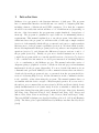
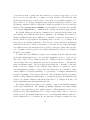
Introduction
MrBayes 3 is a program for the Bayesian inference of phylogeny. The program
has a command-line interface and should run on a variety of computer platforms,
including clusters of Macintosh and UNIX computers. Note that the computer
should be reasonably fast and should have a lot of RAM memory (depending on
the size of the data matrix, the program may require hundreds of megabytes of
memory). The program is optimized for speed and not for minimizing memory
requirements. This manual explains how to use the program. After this section,
which introduces the program, we will first walk you through a simple analysis
(section 2 of the manual), which will get you started, and a more complex analysis
that uses more of the program’s capabilities (section 3). We then briefly describe
the models implemented in the program (section 4), answer some frequently asked
questions (section 5), and discuss the differences between versions 2 and 3 of
the program (section 6). Finally, we give more detailed instructions on how to
compile the program and how to run the parallel versions of it (section 7). Section
7 also contains brief information for developers interested in tweaking MrBayes
code or contributing to the MrBayes project. The manual ends with a series of
diagrams giving a graphical overview of all the models and proposal mechanisms
implemented in the program (Appendix). For more detailed information about
commands and options in MrBayes, see the command reference that can either be
downloaded from the program web site or generated from the program itself (see
section 1.4 Getting Help below). All the information in the command reference
is also available on-line when using the program. The manual assumes that you
are familiar with the basic concepts of Bayesian phylogenetics. If you are new to
the subject, we recommend the recent reviews by Holder and Lewis (2003), Lewis
(2001) and Huelsenbeck et al. (2001, 2002). It is also worthwhile to study the early
papers introducing Bayesian phylogenetic methods (Li 1996; Mau, 1996; Rannala
and Yang, 1996; Mau and Newton, 1997; Rannala and Yang, 1997; Larget and
Simon, 1999; Mau, Newton and Larget, 1999; Newton, Mau and Larget, 1999).
The basic MCMC techniques are described in Metropolis et al. (1953) and Hastings
(1970). The Metropolis-coupled MCMC used by MrBayes was introduced by Geyer
(1991).
5
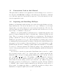
1.1
Conventions Used in this Manual
Throughout the document, we use typewriter font for things you see on screen or
in a data file, and bold font for things you should type in. Alternative commands
you could have typed in, but should not type in to follow the tutorial, are also
given in typewriter font.
1.2
Acquiring and Installing MrBayes
MrBayes 3 is distributed without charge by download from the MrBayes web site,
http://mrbayes.net. If someone has given you a copy of MrBayes 3, we strongly
suggest that you download the most recent version from this site. The site also
gives informationabout the MrBayes users email list and describes how you can
report bugs or contribute to the project.
MrBayes 3 is a plain-vanilla program that uses a command line interface and
therefore behaves virtually the same on all platforms - Macintosh, Windows and
Unix. There is a separate download package for each platform. The Macintosh
package contains two versions of the program: the standard serial version, named
MrBayes3.1 (program icon one copy of Reverend Bayes’s portrait), and a version
for running the program in parallel on clusters of Macintoshes, named MrBayes3.1p
(program icon four portraits of Reverend Bayes). For more information on the
parallel Macintosh version of MrBayes, which requires the installation of POOCH,
see section 7 of this user manual. The Windows package only contains the serial
version of the program and is ready to run after unzipping, just like the Macintosh
serial version.
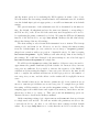
If you decide to run the program under Unix/Linux, then you need to compile
the program from the source code. In the latter case, simply unpack the file
mrbayes3.2 src.tar.gz by typing gunzip MrBayes 3.2 src.tar.gz and then
tar -xf MrBayes 3.2 src.tar . The gunzip command unzips the compressed
file and the tar -xf command extracts all of the files from the .tar archive
that resulted from the unzip operation (note that the .gz suffix is dropped in
the unzip operation). You then need to compile the program. We have included
a “Makefile” that contains compiler instructions producing the serial version of
the program. You simply type make to compile the program according to these
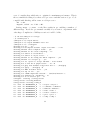
instructions. A typical compile session would look like this:
6
ronquistg5:mrbayes>ls
mrbayes3.2\_src.tar.gz
ronquistg5:mrbayes>gunzip MrBayes\_3.2\_src.tar.gz
ronquistg5:mrbayes>ls
mrbayes3.2\_src.tar
ronquistg5:mrbayes>tar -xf MrBayes\_3.2\_src.tar
ronquistg5:mrbayes>make
gcc -DUNIX\_VERSION -O3 -Wall -Wno-uninitialized -c -o mb.o mb.c
gcc -DUNIX\_VERSION -O3 -Wall -Wno-uninitialized -c -o mcmc.o mcmc.c
gcc -DUNIX\_VERSION -O3 -Wall -Wno-uninitialized -c -o bayes.o bayes.c
gcc -DUNIX\_VERSION -O3 -Wall -Wno-uninitialized -c -o command.o command.c
gcc -DUNIX\_VERSION -O3 -Wall -Wno-uninitialized -c -o mbmath.o mbmath.c
gcc -DUNIX\_VERSION -O3 -Wall -Wno-uninitialized -c -o model.o model.c
gcc -DUNIX\_VERSION -O3 -Wall -Wno-uninitialized -c -o plot.o plot.c
gcc -DUNIX\_VERSION -O3 -Wall -Wno-uninitialized -c -o sump.o sump.c
gcc -DUNIX\_VERSION -O3 -Wall -Wno-uninitialized -c -o sumt.o sumt.c
gcc -DUNIX\_VERSION -O3 -Wall -Wno-uninitialized -lm mb.o bayes.o command.o
mbmath.o mcmc.o model.o plot.o sump.o sumt.o -o mb
ronquistg5:mrbayes>
The compilation usually stops for several minutes at the mcmc.c file; this is
perfectly normal. This is the largest source file and optimization of the code takes
quite a while.
We assume as the default C compiler gcc, which is installed on most systems.
If you do not have gcc installed on your machine, or you want to produce the
MPI version or some other special version of the program, you have to change the
compiler information in the Makefile as described in section 7 of this manual. The
executable serial version of the program is called “mb”. To execute the program,
simply type ./mb in the directory where you compiled the program. The ./ prefix
is needed to tell Unix that you want to run the local copy of mb in your working
directory. If you run MrBayes often, you will probably want to add the program
to your “path”; refer to your Unix manual or your local Unix expert for more
information on this.
All three packages of MrBayes come with example data files. These are intended
to show various types of analyses you can perform with the program, and you can
use them as templates for your own analyses. Two of the files, primates.nex and
cynmix.nex, will be used in the tutorial sections of this manual (sections 2 and 3).
7
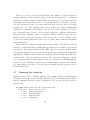
1.3
Getting Started
Start MrBayes by double-clicking the application icon (or typing ./mb ) and you
will see the information below:
MrBayes v3.2-cvs
(Bayesian Analysis of Phylogeny)
Distributed under the GNU General Public License
Type "help" or "help <command>" for information
on the commands that are available.
Type "about" for authorship and general
information about the program.
MrBayes >
The order of the authors is randomized each time you start the program, so
dont be surprised if the order differs from the one above. Note the MrBayes >
prompt at the bottom, which tells you that MrBayes is ready for your commands.
1.4
Changing the Size of the MrBayes Window
Some MrBayes commands will output a lot of information and write fairly long
lines, so you may want to change the size of the MrBayes window to make it
easier to read the output. On Macintosh and Unix machines, you should be able
to increase the window size simply by dragging the margins. On a Windows
machine, you cannot increase the size of the window beyond the preset value by
simply dragging the margins but (on Windows XP, 2000 and NT) you can change
both the size of the screen buffer and the console window by right-clicking on the
blue title bar of the MrBayes window and then selecting “Properties” in the menu
that appears. Make sure the “Layout” tab is selected in the window that appears,
and then set the Screen Buffer Size and Window Size to the desired values.
8
1.5
Getting Help
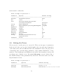
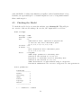
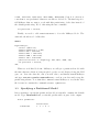
At the MrBayes > prompt, type help to see a list of the commands available
in MrBayes. Most commands allow you to set values (options) for different parameters. If you type help <command> , where <command> is any of the listed
commands, you will see the help information for that command as well as a description of the available options. For most commands, you will also see a list of
the current settings at the end. Try, for instance, help lset or help mcmc . The
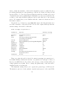
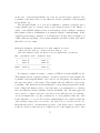
lset settings table looks like this:
Parameter
Options
Current Setting
-----------------------------------------------------------------Nucmodel
4by4/Doublet/Codon/Aa
4by4
Nst
1/2/6
1
Code
Universal/Vertmt/Mycoplasma/
Yeast/Ciliates/Metmt
Universal
Ploidy
Haploid/Diploid
Diploid
Rates
Equal/Gamma/Propinv/Invgamma/Adgamma Equal
Ngammacat
<number>
4
Usegibbs
Yes/No
No
Gibbsfreq
<number>
100
Nbetacat
<number>
5
Omegavar
Equal/Ny98/M3
Equal
Covarion
No/Yes
No
Coding
All/Variable/Noabsencesites/
Nopresencesites
All
Parsmodel
No/Yes
No
------------------------------------------------------------------
Note that MrBayes 3 supports abbreviation of commands and options, so in
many cases it is sufficient to type the first few letters of a command or option
instead of the full name.
A complete list of commands and options is given in the command reference,
which can be downloaded from the program web site (www.mrbayes.net). You
can also produce an ASCII text version of the command reference at any time
by giving the command manual to MrBayes. Further help is available in a set of
hyperlinked html pages produced by Jeff Bates and available on the MrBayes web
site. Finally, you can get in touch with other MrBayes users and developers through
the mrbayes-users email list (subscription information at www.mrbayes.net).
9
1.6
Reporting and Fixing Bugs
If you find a bug in MrBayes, we are very grateful if you tell us about it using
the bug reporting functions of SourceForge, as explained on the MrBayes web site
(www.mrbayes.net). When you submit a bug, make sure that you upload a data
file with the data set and sequence of commands that produced the error. If the
bug occurs during a MCMC analysis (after issuing the “mcmc” command), you
can help us greatly by making sure the bug can be reproduced reliably using a
fixed seed and swapseed for the mcmc command, and ideally also with a small
data set. The Tracker software at SourceForge will make sure that you get email
notification when the bug has been fixed in the source code on the MrBayes CVS
repository at SourceForge. Note, however, that there may be some time before
new executables containing the bug fix will be released.
Advanced users may be interested in fixing bugs themselves in the source code.
Refer to section 7 of this manual for information on how to contribute bug fixes,
improved algorithms or expanded functionality to other users of MrBayes.
1.7
License and Warranty
MrBayes is free software; you can redistribute it and/or modify it under the terms
of the GNU General Public License as published by the Free Software Foundation;
either version 2 of the License, or (at your option) any later version.
The program is distributed in the hope that it will be useful, but WITHOUT
ANY WARRANTY; without even the implied warranty of MERCHANTABILITY
or FITNESS FOR A PARTICULAR PURPOSE. See the GNU General Public
License for more details (http://www.gnu.org/copyleft/gpl.html).
2
Tutorial: A Simple Analysis
This and the fallowing section walks you through two MrBayes example analyses.
The first one describes a simple analysis, and the second one describes how you
set up a more complex analysis of a partitioned data set. The tutorial ends with
some practical tips and advice, as well as some pointers to additional sources of
information.
10
This section is based on the primates.nex data file. It will guide you through
a basic Bayesian MCMC analysis of phylogeny, explaining the most important
features of the program. There are two versions of the tutorial. You will first
find a Quick-Start version for impatient users who want to get an analysis started
immediately. The rest of the section contains a much more detailed description of
the same analysis.
2.1
Quick Start Version
There are four steps to a typical Bayesian phylogenetic analysis using MrBayes:
1. Read the Nexus data file
2. Set the evolutionary model
3. Run the analysis
4. Summarize the samples
In more detail, each of these steps is performed as described in the following
paragraphs:
1. At the MrBayes > prompt, type execute primates.nex. This will bring
the data into the program. When you only give the data file name (primates.nex),
MrBayes assumes that the file is in the current directory. If this is not the case,
you have to use the full or relative path to your data file, for example execute
../taxa/primates.nex. If you are running your own data file for this tutorial,
beware that it may contain some MrBayes commands that can change the behavior
of the program; delete those commands or put them in square brackets to follow
this tutorial.
2. At the MrBayes > prompt, type lset nst=6 rates=invgamma. This sets
the evolutionary model to the GTR model with gamma-distributed rate variation
across sites and a proportion of invariable sites. If your data are not DNA or RNA,
if you want to invoke a different model, or if you want to use non-default priors,
refer to the full MrBayes manual and its Appendix.
3.1. At the MrBayes > prompt, type mcmc ngen=20000. This will ensure
that you get at least 200 samples from the posterior probability distribution, since
the default sampling frequency is every 100th generation. For larger data sets
11
you probably want to run the analysis longer and sample less frequently. You can
find the predicted remaining time to completion of the analysis in the last column
printed to screen.
3.2. If the standard deviation of split frequencies is below 0.01 after 20,000
generations, stop the run by answering no when the program asks Continue the
analysis? (yes/no). Otherwise, keep adding generations until the value falls
below 0.01. If you are interested mainly in the well-supported parts of the tree, a
standard deviation below 0.05 may be adequate.
4.1. Type sump relburnin=yes burninfrac=0.25 to summarize the parameter values using the same burn-in as the mcmc command. The program will
output a table with summaries of the samples of the substitution model parameters, including the mean, mode, and 95 % credibility interval (region of Highest
Posterior Density, HPD) of each parameter. Make sure that the potential scale
reduction factor (PSRF) is reasonably close to 1.0 for all parameters; if not, you
need to run the analysis longer.
4.2. Summarize the trees by typing sumt relburnin=yes burninfrac=0.25.
The program will output a cladogram with the posterior probabilities for each split
and a phylogram with mean branch lengths. The trees will also be printed to a file
that can be read by FigTree and other tree-drawing programs, such as TreeView
and Mesquite.
It does not have to be more complicated than this; however, as you get more
proficient you will probably want to know more about what is happening behind
the scenes. The rest of this section explains each of the steps in more detail and
introduces you to all the implicit assumptions you are making and the machinery
that MrBayes uses in order to perform your analysis.
2.2
Getting Data into MrBayes
To get data into MrBayes, you need a so-called Nexus file that contains aligned
nucleotide or amino acid sequences, morphological (”standard”) data, restriction
site (binary) data, or any mix of these four data types. The Nexus data file is often
generated by another program, such as Mesquite. Note, however, that MrBayes
version 3 does not support the full Nexus standard, so you may have to do a
little editing of the file for MrBayes to process it properly. In particular, MrBayes
12
uses a fixed set of symbols for each data type and does not support user-defined
symbols. The supported symbols are {A, C, G, T, R, Y, M, K, S, W, H, B, V,
D, N} for DNA data, {A, C, G, U, R, Y, M, K, S, W, H, B, V, D, N} for RNA
data, {A, R, N, D, C, Q, E, G, H, I, L, K, M, F, P, S, T, W, Y, V, X} for protein
data, {0, 1} for restriction (binary) data, and {0, 1, 2, 3, 4, 5, 6, 5, 7, 8, 9} for
standard (morphology) data. In addition to the standard one-letter ambiguity
symbols for DNA and RNA listed above, ambiguity can also be expressed using
the Nexus parenthesis or curly braces notation. For instance, a taxon polymorphic
for states 2 and 3 can be coded as (23), (2,3), {23}, or {2,3} and a taxon with
either amino acid A or F can be coded as (AF), (A,F), {AF} or {A,F}. Like most
other statistical phylogenetics programs, MrBayes effectively treats polymorphism
and uncertainty the same way (as uncertainty), so it does not matter whether you
use parentheses or curly braces. If you have other symbols in your matrix than
the ones supported by MrBayes, you need to replace them before processing the
data block in MrBayes. You also need to remove the ”Equate” and ”Symbols”
statements in the ”Format” line if they are included. Unlike the Nexus standard,
MrBayes supports data blocks that contain mixed data types as described below.
To put the data into MrBayes type execute <filename> at the MrBayes >
prompt, where <filename> is the name of the input file. To process our example
file, type execute primates.nex or simply exe primates.nex to save some typing (MrBayes allows you to use the shortest unambiguous version of a command).
Note that the input file must be located in the same folder (directory) where you
started the MrBayes application (or else you will have to give the path to the file)
and the name of the input file should not have blank spaces, or it will have to be
quoted. If everything proceeds normally, MrBayes will acknowledge that it has
read the data in the DATA block of the Nexus file by outputting some information
about the file read in.
2.3
Specifying a Model
All of the commands are entered at the MrBayes > prompt. At a minimum two
commands, lset and prset, are required to specify the evolutionary model that
will be used in the analysis. Usually, it is also a good idea to check the model
settings prior to the analysis using the showmodel command. In general, lset is
13
used to define the structure of the model and prset is used to define the prior
probability distributions on the parameters of the model. In the following, we will
specify a GTR + I + Γ model (a General Time Reversible model with a proportion
of invariable sites and a gamma-shaped distribution of rates across sites) for the
evolution of the mitochondrial sequences and we will check all of the relevant
priors. We assume that you are familiar with the common stochastic models of
molecular evolution.
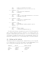
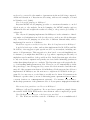
In general, a good start is to type help lset. Ignore the help information for
now and concentrate on the table at the bottom of the output, which specifies the
current settings. It should look like this:
Model settings for partition 1:
Parameter
Options
Current Setting
-----------------------------------------------------------------Nucmodel
4by4/Doublet/Codon
4by4
Nst
1/2/6
1
Code
Universal/Vertmt/Mycoplasma/
Yeast/Ciliates/Metmt
Universal
Ploidy
Haploid/Diploid
Diploid
Rates
Equal/Gamma/Propinv/Invgamma/Adgamma Equal
Ngammacat
<number>
4
Usegibbs
Yes/No
No
Gibbsfreq
<number>
100
Nbetacat
<number>
5
Omegavar
Equal/Ny98/M3
Equal
Covarion
No/Yes
No
Coding
All/Variable/Noabsencesites/
Nopresencesites
All
Parsmodel
No/Yes
No
------------------------------------------------------------------
First, note that the table is headed by Model settings for partition 1.
By default, MrBayes divides the data into one partition for each type of data you
have in your DATA block. If you have only one type of data, all data will be in
a single partition by default. How to change the partitioning of the data will be
explained in the second tutorial.
The Nucmodel setting allows you to specify the general type of DNA model.
The Doublet option is for the analysis of paired stem regions of ribosomal DNA
14
and the Codon option is for analyzing the DNA sequence in terms of its codons.
We will analyze the data using a standard nucleotide substitution model, in which
case the default 4by4 option is appropriate, so we will leave Nucmodel at its default
setting.
The general structure of the substitution model is determined by the Nst setting. By default, all substitutions have the same rate (Nst=1), corresponding to
the F81 model (or the JC model if the stationary state frequencies are forced to
be equal using the prset command, see below). We want the GTR model (Nst=6)
instead of the F81 model so we type lset nst=6. MrBayes should acknowledge
that it has changed the model settings.
The Code setting is only relevant if the Nucmodel is set to Codon. The Ploidy
setting is also irrelevant for us. However, we need to change the Rates setting
from the default Equal (no rate variation across sites) to Invgamma (gammashaped rate variation with a proportion of invariable sites). Do this by typing
lset rates=invgamma. Again, MrBayes will acknowledge that it has changed
the settings. We could have changed both lset settings at once if we had typed
lset nst=6 rates=invgamma in a single line.
We will leave the Ngammacat setting (the number of discrete categories used to
approximate the gamma distribution) at the default of 4. In most cases, four rate
categories are sufficient. It is possible to increase the accuracy of the likelihood
calculations by increasing the number of rate categories. However, the time it will
take to complete the analysis will increase in direct proportion to the number of
rate categories you use, and the effects on the results will be negligible in most
cases.
The default behaviour for the discrete gamma model of rate variation across
sites is to sum site probabilities across rate categories. To sample those probabilities using a Gibbs sampler, we can set the Usegibbs setting to Yes. The Gibbs
sampling approach is much faster and requires less memory, but it has some implications you have to be aware of. This option and the Gibbsfreq option are
discussed in more detail in the MrBayes manual.
Of the remaining settings, it is only Covarion and Parsmodel that are relevant
for single nucleotide models. We will use neither the parsimony model nor the
covariotide model for our data, so we will leave these settings at their default
values. If you type help lset now to verify that the model is correctly set, the
15
table should look like this:
Model settings for partition 1:
Parameter
Options
Current Setting
-----------------------------------------------------------------Nucmodel
4by4/Doublet/Codon
4by4
Nst
1/2/6
6
Code
Universal/Vertmt/Mycoplasma/
Yeast/Ciliates/Metmt
Universal
Ploidy
Haploid/Diploid
Diploid
Rates
Equal/Gamma/Propinv/Invgamma/Adgamma Invgamma
Ngammacat
<number>
4
Usegibbs
Yes/No
No
Gibbsfreq
<number>
100
Nbetacat
<number>
5
Omegavar
Equal/Ny98/M3
Equal
Covarion
No/Yes
No
Coding
All/Variable/Noabsencesites/
Nopresencesites
All
Parsmodel
No/Yes
No
------------------------------------------------------------------
2.4
Setting the Priors
We now need to set the priors for our model. There are six types of parameters
in the model: the topology, the branch lengths, the four stationary frequencies
of the nucleotides, the six different nucleotide substitution rates, the proportion
of invariable sites, and the shape parameter of the gamma distribution of rate
variation. The default priors in MrBayes work well for most analyses, and we will
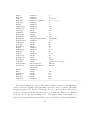
not change any of them for now. By typing help prset you can obtain a list of
the default settings for the parameters in your model. The table at the end of the
help information reads:
Model settings for partition 1:
Parameter
Options
Current Setting
-----------------------------------------------------------------Tratiopr
Beta/Fixed
Beta(1.0,1.0)
Revmatpr
Dirichlet/Fixed
Dirichlet(1.0,1.0,1.0,1.0,1.0,1.0)
16
Aamodelpr
Aarevmatpr
Omegapr
Ny98omega1pr
Ny98omega3pr
M3omegapr
Codoncatfreqs
Statefreqpr
Shapepr
Ratecorrpr
Pinvarpr
Covswitchpr
Symdirihyperpr
Topologypr
Brlenspr
Treeheightpr
Speciationpr
Extinctionpr
Sampleprob
Thetapr
Nodeagepr
Treeagepr
Fixed/Mixed
Fixed(Poisson)
Dirichlet/Fixed
Dirichlet(1.0,1.0,...)
Dirichlet/Fixed
Dirichlet(1.0,1.0)
Beta/Fixed
Beta(1.0,1.0)
Uniform/Exponential/Fixed
Exponential(1.0)
Exponential/Fixed
Exponential
Dirichlet/Fixed
Dirichlet(1.0,1.0,1.0)
Dirichlet/Fixed
Dirichlet(1.0,1.0,1.0,1.0)
Uniform/Exponential/Fixed
Uniform(0.0,200.0)
Uniform/Fixed
Uniform(-1.0,1.0)
Uniform/Fixed
Uniform(0.0,1.0)
Uniform/Exponential/Fixed
Uniform(0.0,100.0)
Uniform/Exponential/Fixed
Fixed(Infinity)
Uniform/Constraints/Fixed
Uniform
Unconstrained/Clock/Fixed
Unconstrained:Exp(10.0)
Exponential/Gamma
Exponential(1.0)
Uniform/Exponential/Fixed
Uniform(0.0,10.0)
Uniform/Exponential/Fixed
Uniform(0.0,10.0)
<number>
1.00
Uniform/Exponential/Fixed
Uniform(0.0,10.0)
Unconstrained/Calibrated
Unconstrained
Fixed/Uniform/
Offsetexponential
Fixed(1.00)
Clockratepr
Strict/Cpp/Bm/Ibr
Strict
Cppratepr
Fixed/Exponential
Exponential(0.10)
Psigammapr
Fixed/Exponential/Uniform
Fixed(1.00)
Nupr
Fixed/Exponential/Uniform
Fixed(1.00)
Ratepr
Fixed/Variable=Dirichlet
Fixed
------------------------------------------------------------------
We need to focus on Revmatpr (for the six substitution rates of the GTR rate
matrix), Statefreqpr (for the stationary nucleotide frequencies of the GTR rate
matrix), Shapepr (for the shape parameter of the gamma distribution of rate
variation), Pinvarpr (for the proportion of invariable sites), Topologypr (for the
topology), and Brlenspr (for the branch lengths).
The default prior probability density is a flat Dirichlet (all values are 1.0) for
both Revmatpr and Statefreqpr. This is appropriate if we want estimate these
parameters from the data assuming no prior knowledge about their values. It is
possible to fix the rates and nucleotide frequencies but this is generally not recommended. However, it is occasionally necessary to fix the nucleotide frequencies
to be equal, for instance in specifying the JC and SYM models. This would be
17
achieved by typing prset statefreqpr=fixed(equal).
If we wanted to specify a prior that put more emphasis on equal nucleotide
frequencies than the default flat Dirichlet prior, we could for instance use prset
statefreqpr = Dirichlet(10,10,10,10) or, for even more emphasis on equal
frequencies, prset statefreqpr=Dirichlet(100,100,100,100). The sum of the
numbers in the Dirichlet distribution determines how focused the distribution is,
and the balance between the numbers determines the expected proportion of each
nucleotide (in the order A, C, G, and T). Usually, there is a connection between the
parameters in the Dirichlet distribution and the observations. For example, you
can think of a Dirichlet (150,100,90,140) distribution as one arising from observing
(roughly) 150 A’s, 100 C’s, 90 G’s and 140 T’s in some set of reference sequences.
If the reference sequences are independent but clearly relevant to the analysis of
your sequences, it might be reasonable to use those numbers as a prior in your
analysis.
In our analysis, we will be cautious and leave the prior on state frequencies at its
default setting. If you have changed the setting according to the suggestions above,
you need to change it back by typing prset statefreqpr=Dirichlet(1,1,1,1) or
prs st = Dir(1,1,1,1) if you want to save some typing. Similarly, we will leave the
prior on the substitution rates at the default flat Dirichlet(1,1,1,1,1,1) distribution.
The Shapepr parameter determines the prior for the α (shape) parameter of
the gamma distribution of rate variation. We will leave it at its default setting,
a uniform distribution spanning a wide range of α values. The prior for the proportion of invariable sites is set with Pinvarpr. The default setting is a uniform
distribution between 0 and 1, an appropriate setting if we don’t want to assume
any prior knowledge about the proportion of invariable sites.
For topology, the default Uniform setting for the Topologypr parameter puts
equal probability on all distinct, fully resolved topologies. The alternative is to
constrain some nodes in the tree to always be present but we will not attempt that
in this analysis.
The Brlenspr parameter can either be set to unconstrained or clock-constrained.
For trees without a molecular clock (unconstrained) the branch length prior can be
set either to exponential or uniform. The default exponential prior with parameter
10.0 should work well for most analyses. It has an expectation of 1/10 = 0.1 but
allows a wide range of branch length values (theoretically from 0 to infinity). Be18
cause the likelihood values vary much more rapidly for short branches than for long
branches, an exponential prior on branch lengths is closer to being uninformative
than a uniform prior.
2.5
Checking the Model
To check the model before we start the analysis, type showmodel. This will give
an overview of the model settings. In our case, the output will be as follows:
Model settings:
Datatype
Nucmodel
Nst
Covarion
# States
Rates
= DNA
= 4by4
= 6
Substitution rates, expressed as proportions
of the rate sum, have a Dirichlet prior
(1.00,1.00,1.00,1.00,1.00,1.00)
= No
= 4
State frequencies have a Dirichlet prior
(1.00,1.00,1.00,1.00)
= Invgamma
Gamma shape parameter is uniformly distributed on the interval (0.00,200.00).
Proportion of invariable sites is uniformly distributed on the interval (0.00,1.00).
Gamma distribution is approximated using 4 categories.
Likelihood summarized over all rate categories in each generation.
Active parameters:
Parameters
-----------------Revmat
1
Statefreq
2
Shape
3
Pinvar
4
Topology
5
Brlens
6
-----------------1 --
Parameter
= Revmat
19
Type
Prior
= Rates of reversible rate matrix
= Dirichlet(1.00,1.00,1.00,1.00,1.00,1.00)
2 --
Parameter
Type
Prior
= Pi
= Stationary state frequencies
= Dirichlet
3 --
Parameter
Type
Prior
= Alpha
= Shape of scaled gamma distribution of site rates
= Uniform(0.00,200.00)
4 --
Parameter
Type
Prior
= Pinvar
= Proportion of invariable sites
= Uniform(0.00,1.00)
5 --
Parameter
Type
Prior
Subparam.
=
=
=
=
6 --
Parameter
Type
Prior
= V
= Branch lengths
= Unconstrained:Exponential(10.0)
Tau
Topology
All topologies equally probable a priori
V
Note that we have six types of parameters in our model. All of these parameters
will be estimated during the analysis (to fix them to some estimated values, use
the prset command and specify a fixed prior). To see more information about
each parameter, including its starting value, use the showparams command. The
startvals command allows one to set the starting values of each chain separately.
2.6
Setting up the Analysis
The analysis is started by issuing the mcmc command. However, before doing this,
we recommend that you review the run settings by typing help mcmc. In our
case, we will get the following table at the bottom of the output:
Parameter
Options
Current Setting
----------------------------------------------------Seed
<number>
1141605343
Swapseed
<number>
1280372787
Ngen
<number>
1000000
20
Nruns
Nchains
Temp
Reweight
Swapfreq
Nswaps
Samplefreq
Printfreq
Printall
Printmax
Mcmcdiagn
Diagnfreq
Diagnstat
Minpartfreq
Allchains
Allcomps
Relburnin
Burnin
Burninfrac
Stoprule
Stopval
Savetrees
Checkpoint
Checkfreq
Filename
Startparams
Starttree
<number>
2
<number>
4
<number>
0.200000
<number>,<number>
0.00 v 0.00 ^
<number>
1
<number>
1
<number>
100
<number>
100
Yes/No
Yes
<number>
8
Yes/No
Yes
<number>
1000
Avgstddev/Maxstddev
Avgstddev
<number>
0.10
Yes/No
No
Yes/No
No
Yes/No
Yes
<number>
0
<number>
0.25
Yes/No
No
<number>
0.05
Yes/No
No
Yes/No
Yes
<number>
100000
<name>
primates.nex.<p/t>
Current/Reset
Current
Current/Random/
Current
Parsimony
Nperts
<number>
0
Data
Yes/No
Yes
Ordertaxa
Yes/No
No
Append
Yes/No
No
Autotune
Yes/No
Yes
Tunefreq
<number>
100
---------------------------------------------------------------------------
The Seed is simply the seed for the random number generator, and Swapseed
is the seed for the separate random number generator used to generate the chain
swapping sequence (see below). Unless they are set to user-specified values, these
seeds are generated from the system clock, so your values are likely to be different
from the ones in the screen dump above. The Ngen setting is the number of
generations for which the analysis will be run. It is useful to run a small number
21
of generations first to make sure the analysis is correctly set up and to get an
idea of how long it will take to complete a longer analysis. We will start with
20,000 generations but you may want to start with an even smaller number for a
larger data set. To change the Ngen setting without starting the analysis we use
the mcmcp command, which is equivalent to mcmc except that it does not start the
analysis. Type mcmcp ngen=20000 to set the number of generations to 20,000.
You can type help mcmc to confirm that the setting was changed appropriately.
By default, MrBayes will run two simultaneous, completely independent analyses starting from different random trees (Nruns = 2). Running more than one
analysis simultaneously allows MrBayes to calculate convergence diagnostics on
the fly, which is very helpful in determining when you have a good sample from
the posterior probability distribution. The idea is to start each run from different
randomly chosen trees. In the early phases of the run, the two runs will sample
very different trees but when they have reached convergence (when they produce
a good sample from the posterior probability distribution), the two tree samples
should be very similar.
To make sure that MrBayes compares tree samples from the different runs,
check that Mcmcdiagn is set to yes and that Diagnfreq is set to some reasonable value, such as every 1000th generation. MrBayes will now calculate various run diagnostics every Diagnfreq generation and print them to a file with the
name <Filename>.mcmc. The most important diagnostic, a measure of the similarity of the tree samples in the different runs, will also be printed to screen
every Diagnfreq generation. Every time the diagnostics are calculated, either
a fixed number of samples (burnin) or a percentage of samples (burninfrac)
from the beginning of the chain is discarded. The relburnin setting determines
whether a fixed burnin (relburnin=no) or a burnin percentage (relburnin=yes)
is used. By default, MrBayes will discard the first 25 % samples from the cold
chain (relburnin=yes and burninfrac=0.25).
By default, MrBayes uses Metropolis coupling to improve the MCMC sampling
of the target distribution. The Swapfreq, Nswaps, Nchains, and Temp settings
together control the Metropolis coupling behavior. When Nchains is set to 1, no
heating is used. When Nchains is set to a value n larger than 1, then n − 1 heated
chains are used. By default, Nchains is set to 4, meaning that MrBayes will use 3
heated chains and one ”cold chain. In our experience, heating is essential for some
22
data sets but it is not needed for others. Adding more than three heated chains
may be helpful in analyzing large and difficult data sets. The time complexity of
the analysis is directly proportional to the number of chains used (unless MrBayes
runs out of physical RAM memory, in which case the analysis will suddenly become
much slower), but the cold and heated chains can be distributed among processors
in a cluster of computers and among cores in multicore processors using the MPI
version of the program, greatly speeding up the calculations.
MrBayes uses an incremental heating scheme, in which chain i is heated by
raising its posterior probability to the power 1/(1+iλ), where λ is the temperature
controlled by the Temp parameter. Every Swapfreq generation, two chains are
picked at random and an attempt is made to swap their states. For many analyses,
the default settings should work nicely. If you are running many more than three
heated chains, however, you may want to increase the number of swaps (Nswaps)
that are tried each time the chain stops for swapping. If the frequency of swapping
between chains that are adjacent in temperature is low, you may want to decrease
the Temp parameter.
The Samplefreq setting determines how often the chain is sampled. By default,
the chain is sampled every 100th generation, and this works well for most analyses,
including ours. If you have a large data set, it may take longer to converge and
you may want to sample less frequently or you will end up with very large files
containing tree and parameter samples.
When the chain is sampled, the current values of the model parameters are
printed to file. The substitution model parameters are printed to a .p file (in our
case, there will be one file for each independent analysis, and they will be called
primates.nex.run1.p and primates.nex.run2.p). The .p files are tab delimited
text files that can be imported into most statistics and graphing programs. The
topology and branch lengths are printed to a .t file (in our case, there will be two
files called primates.nex.run1.t and primates.nex.run2.t). The .t files are
Nexus tree files that can be imported into programs like PAUP* and TreeView.
The root of the .p and .t file names can be altered using the Filename setting.
The Printfreq parameter controls the frequency with which the state of the
chains is printed to screen. You can leave Printfreq at the default value (print
to screen every 100th generation).
23
When you set up your model and analysis (the number of runs and heated
chains), MrBayes creates starting values for the model parameters. A different
random tree with predefined branch lengths is generated for each chain and most
substitution model parameters are set to predefined values. For instance, stationary state frequencies start out being equal and unrooted trees have all branch
lengths set to 0.1. The starting values can be changed by using the Startvals
command. For instance, user-defined trees can be read into MrBayes by executing a Nexus file with a ”trees” block and then assigned to different chains using
the Startvals command. After a completed analysis, MrBayes keeps the parameter values of the last generation and will use those as the starting values
for the next analysis unless the values are reset using mcmc starttrees=random
startvals=reset.
Since version 3.2, MrBayes prints all parameter values of all chains (cold and
heated) to a checkpoint file every Checkfreq generations, by default every 100, 000
generations. The checkpoint file has the suffix .ckp. If you run an analysis and it
is stopped prematurely, you can restart it from the last checkpoint by using mcmc
append=yes. MrBayes will start the new analysis from the checkpoint; it will even
read in all the old trees and include them in the convergence diagnostic. At the
end of the new run, you will parameter and tree files that are indistinguishable
from those you would have obtained from an uninterrupted analysis. Our data set
is so small that we are likely to get an adequate sample from the posterior before
the first checkpoint.
2.7
Running the Analysis
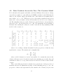
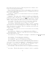
Finally, we are ready to start the analysis. Type mcmc. MrBayes will first print
information about the model and then list the proposal mechanisms that will be
used in sampling from the posterior distribution. In our case, the proposals are
the following:
The MCMC sampler will use the following moves:
With prob. Chain will use move
1.79 %
Dirichlet(Revmat)
1.79 %
Slider(Revmat)
1.79 %
Dirichlet(Pi)
1.79 %
Slider(Pi)
24
3.57
17.86
17.86
35.71
17.86
%
%
%
%
%
Multiplier(Alpha)
eSS(Tau,V)
eTBR(Tau,V)
pSPR(Tau,V)
Multiplier(V)
The exact set of proposals and their relative probabilities may differ depending
on the exact version of the program that you are using. Note that MrBayes
will spend most of its effort changing the topology (Tau) and branch length (V)
parameters. In our experience, topology and branch lengths are the most difficult
parameters to integrate over and we therefore let MrBayes spend a large proportion
of its time proposing new values for those parameters. The proposal probabilities
and tuning parameters can be changed with the Propset command, but be warned
that inappropriate changes of these settings may destroy any hopes of achieving
convergence.
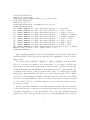
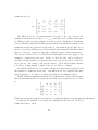
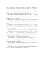
After the initial log likelihoods, MrBayes will print the state of the chains every
100th generation, like this:
Chain results:
1 -- (-7515.474) (-7815.502) (-7571.894) [-7511.216] * (-7912.443) (-7430.324) (-7722.968) [-7559.768]
100 -- (-6457.486) (-6443.204) (-6362.653) [-6380.948] * (-6452.131) (-6412.384) (-6460.409) [-6335.541] -200 -- (-6372.894) (-6284.653) [-6212.481] (-6320.671) * (-6326.804) [-6206.832] (-6368.248) (-6274.370) -300 -- (-6215.251) (-6238.351) [-6173.761] (-6215.648) * [-6175.548] (-6162.354) (-6295.342) (-6170.237) -400 -- (-6169.260) [-6106.352] (-6157.140) (-6134.522) * [-6044.984] (-6105.105) (-6239.651) (-6126.382) -500 -- (-6132.093) [-6045.345] (-6071.921) (-6105.350) * [-6027.764] (-6052.897) (-6122.643) (-6054.535) -600 -- (-6086.736) [-5966.605] (-6022.943) (-6048.775) * (-6005.907) (-6050.838) (-6052.809) [-5987.512] -700 -- (-6071.156) [-5949.411] (-6001.893) (-6028.975) * (-5969.434) (-6034.590) (-5985.207) [-5962.131] -800 -- (-6043.289) [-5919.917] (-5955.320) (-5990.842) * (-5934.204) (-5998.712) [-5917.514] (-5957.886) -900 -- (-6036.192) [-5915.292] (-5940.829) (-5928.622) * (-5916.117) (-5974.419) [-5885.179] (-5947.285) -1000 -- (-6033.926) [-5879.274] (-5930.137) (-5912.750) * (-5919.677) (-5979.409) [-5849.042] (-5893.568) --
0:00:00
0:01:39
0:01:05
0:01:38
0:01:18
0:01:04
0:01:22
0:01:12
0:01:03
0:01:16
Average standard deviation of split frequencies: 0.000000
1100 -- (-6015.382) (-5879.918) (-5932.478) [-5850.292] * (-5845.497) (-5970.688) [-5835.631] (-5882.916) -- 0:01:08
...
19000 -- (-5725.208) (-5728.059) (-5723.771) [-5720.516] * (-5725.163) (-5733.313) (-5731.771) [-5733.018] -- 0:00:03
Average standard deviation of split frequencies: 0.000000
19100
19200
19300
19400
19500
19600
19700
19800
19900
20000
-----------
(-5721.777)
(-5725.644)
(-5722.932)
(-5722.253)
[-5723.923]
(-5731.034)
(-5738.424)
(-5732.570)
(-5724.326)
(-5723.983)
(-5731.432)
[-5723.736]
(-5727.877)
(-5732.094)
(-5732.401)
(-5729.754)
(-5731.187)
(-5732.026)
(-5728.367)
(-5727.877)
[-5724.683]
(-5730.977)
(-5729.790)
(-5733.256)
(-5726.903)
(-5732.244)
(-5728.800)
(-5729.572)
[-5725.441]
[-5724.582]
(-5719.899)
(-5718.788)
[-5719.233]
[-5721.040]
(-5722.455)
[-5725.747]
[-5728.881]
[-5727.604]
(-5726.584)
(-5720.923)
*
*
*
*
*
*
*
*
*
*
(-5724.676)
[-5732.428]
[-5728.970]
(-5731.382)
(-5727.740)
(-5725.214)
(-5725.340)
[-5721.525]
(-5723.621)
(-5730.172)
[-5725.091]
(-5725.226)
(-5732.444)
[-5726.897]
(-5722.413)
(-5722.015)
[-5720.537]
(-5718.952)
(-5730.548)
(-5728.091)
(-5728.996)
(-5733.051)
(-5730.074)
(-5734.551)
(-5736.126)
(-5733.053)
(-5734.678)
(-5741.802)
(-5746.447)
(-5748.344)
(-5742.658)
(-5741.748)
(-5731.851)
(-5733.469)
[-5727.055]
[-5723.926]
(-5725.685)
(-5722.740)
[-5716.807]
[-5716.947]
-----------
0:00:03
0:00:02
0:00:02
0:00:02
0:00:01
0:00:01
0:00:01
0:00:00
0:00:00
0:00:00
Average standard deviation of split frequencies: 0.000520
Continue with analysis? (yes/no): no
If you have the terminal window wide enough, each generation of the chain will
print on a single line.
25
The first column lists the generation number. The following four columns with
negative numbers each correspond to one chain in the first run. Each column
corresponds to one physical location in computer memory, and the chains actually
shift positions in the columns as the run proceeds. The numbers are the log
likelihood values of the chains. The chain that is currently the cold chain has its
value surrounded by square brackets, whereas the heated chains have their values
surrounded by parentheses. When two chains successfully change states, they
trade column positions (places in computer memory). If the Metropolis coupling
works well, the cold chain should move around among the columns; this means
that the cold chain successfully swaps states with the heated chains. If the cold
chain gets stuck in one of the columns, then the heated chains are not successfully
contributing states to the cold chain, and the Metropolis coupling is inefficient.
The analysis may then have to be run longer. You can also try to reduce the
temperature difference between chains, which may increase the efficiency of the
Metropolis coupling.
The star column separates the two different runs. The last column gives the
time left to completion of the specified number of generations. This analysis approximately takes 1 second per 100 generations. Because different moves are used
in each generation, the exact time varies somewhat for each set of 100 generations,
and the predicted time to completion will be unstable in the beginning of the run.
After a while, the predictions will become more accurate and the time will decrease
predictably.
2.8
When to Stop the Analysis
At the end of the run, MrBayes asks whether or not you want to continue with the
analysis. Before answering that question, examine the average standard deviation
of split frequencies. As the two runs converge onto the stationary distribution,
we expect the average standard deviation of split frequencies to approach zero,
reflecting the fact that the two tree samples become increasingly similar. In our
case, the average standard deviation is down to 0.0 already after 1,000 generations
and then stays at very low values throughout the run. Your values can differ
slightly because of stochastic effects but should show a similar trend.
In larger and more difficult analyses, you will typically see the standard devi-
26
ation of split frequencies come down much more slowly towards 0.0; the standard
deviation can even increase temporarily, especially in the early part of the run.
A rough guide is that an average standard deviation below 0.01 is very good
indication of convergence, while values between 0.01 and 0.05 may be adequate
depending on the purpose of your analysis. The sumt command (see below) allows
you to examine the error (standard deviation) associated with each clade in the
tree. Typically, most of the error is associated with clades that are not very well
supported (posterior probabilities well below 0.95), and getting accurate estimates
of those probabilities may not be an important concern.
Given the extremely low value of the average standard deviation at the end
of the run, there appears to be no need to continue the analysis beyond 20,000
generations so when MrBayes asks Continue with analysis? (yes/no): stop
the analysis by typing no.
Although we recommend using a convergence diagnostic, such as the standard
deviation of split frequencies, there are also simpler but less powerful methods of
determining when to stop the analysis. The simplest technique is to examine the
log likelihood values (or, more exactly, the log probability of the data given the
parameter values) of the cold chain, that is, the values printed to screen within
square brackets. In the beginning of the run, the values typically increase rapidly
(the absolute values decrease, since these are negative numbers). In our case, the
values increase from below −7500 to around −5725 in the first few thousand generations. This is the ”burn-in” phase and the corresponding samples are typically
discarded. Once the likelihood of the cold chain stops to increase and starts to
randomly fluctuate within a more or less stable range, the run may have reached
stationarity, that is, it may be producing a good sample from the posterior probability distribution. At stationarity, we also expect different, independent runs
to sample similar likelihood values. Trends in likelihood values can be deceiving
though; you’re more likely to detect problems with convergence by comparing split
frequencies than by looking at likelihood trends.
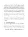
When you stop the analysis, MrBayes will print several types of information
useful in optimizing the analysis. This is primarily of interest if you have difficulties
in obtaining convergence, which is unlikely to happen with this analysis. We give
a few tips on how to improve convergence at the end of the tutorial.
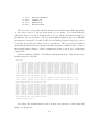
27
2.9
Summarizing Samples of Substitution Model Parameters
During the run, samples of the substitution model parameters have been written
to the .p files every samplefreq generation. These files are tab-delimited text
files that look something like this (numbers are actually given in scientific format
by default, so the files do not look quite as nice as the one below although they
are structurally equivalent):
[ID: 9409050143]
Gen
LnL
1
-7821.374
100
-6328.159
....
19900
-5723.107
20000
-5720.765
TL
2.100
2.091
r(A<->C)
0.166667
0.166667
...
...
...
pi(T)
0.250000
0.307263
alpha
0.500000
0.842091
pinvar
0.000000
0.036693
2.990
2.959
0.048609
0.048609
...
...
0.251888
0.240826
0.605319
0.636716
0.152817
0.180024
The first number, in square brackets, is a randomly generated ID number that
lets you identify the analysis from which the samples come. The next line contains
the column headers, and is followed by the sampled values. From left to right, the
columns contain: (1) the generation number (Gen); (2) the log likelihood of the
cold chain (LnL); (3) the total tree length (the sum of all branch lengths, TL); (4)
the six GTR rate parameters (r(A<->C), r(A<->G) etc); (5) the four stationary
nucleotide frequencies (pi(A), pi(C) etc); (6) the shape parameter of the gamma
distribution of rate variation (alpha); and (7) the proportion of invariable sites
(pinvar). If you use a different model for your data set, the .p files will of course
be different.
MrBayes provides the sump command to summarize the sampled parameter
values. Before using it, we need to decide on the burn-in. Since the convergence
diagnostic we used previously to determine when to stop the analysis discarded
the first 25 % of the samples, it makes sense to discard 25 % of the samples when
summarizing the parameter values. Thus, summarize the information in the .p file
by typing sump reburnin=yes burnin=0.25. By default, sump will summarize
the information in the .p file or files generated most recently, but the filename
can be changed if necessary. The relburnin=yes option specifies that we want to
give the burn-in in terms of a fraction (relative burn-in) rather than as an absolute
value. The burninfrac option specifies the desired burn-in fraction.
28
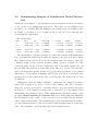
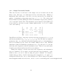
The sump command will first generate a plot of the generation versus the log
probability of the data (the log likelihood values). If we are at stationarity, this
plot should look like ”white noise”, that is, there should be no tendency of increase
or decrease over time. The plot should look something like this:
+------------------------------------------------------------+ -5717.71
|
2
1
1
2|
|
1
1
|
|
2 2
1
1
1 |
|22 2
1
12
1
|
|
22
2
1
1
1
2 1 1
1
2
|
|11
1111
1
1
112
1
2
12
1
|
| 1
*
22
2
1
1*
2
2 |
| 2 1 1
1
1 2*
12
2
12
1
|
|
221 2
12 2
* 2
2
2 1
2
1|
|
2
1 2 *
2
1
1 2 2 2 2
1 |
|
1
1
2 2 11
1
|
|
2 2
2
2
2
12 2 |
|
2
2
|
|
2
|
|
1
1
2
|
+------+-----+-----+-----+-----+-----+-----+-----+-----+-----+ -5731.34
^
^
5000
20000
If you see an obvious trend in your plot, either increasing or decreasing, you
very likely need to run the analysis longer to get an adequate sample from the
posterior probability distribution.
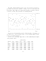
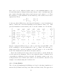
At the bottom of the sump output, there is a table summarizing the samples
of the parameter values:
95% HPD Interval
-------------------Parameter
Mean
Variance
Lower
Upper
Median
PSRF+
-----------------------------------------------------------------------------TL
2.925036
0.067504
2.415013
3.379712
2.928130
0.997
r(A<->C)
0.046638
0.000087
0.025996
0.061754
0.047223
1.033
r(A<->G)
0.472949
0.001944
0.380185
0.538198
0.475733
1.093
r(A<->T)
0.038436
0.000070
0.024704
0.057508
0.037291
1.067
r(C<->G)
0.028027
0.000145
0.005312
0.049157
0.028217
1.023
r(C<->T)
0.394395
0.001729
0.319370
0.473755
0.390730
1.110
r(G<->T)
0.019556
0.000169
0.000078
0.044754
0.017799
1.018
pi(A)
0.355732
0.000173
0.333218
0.383760
0.354468
1.064
pi(C)
0.317528
0.000128
0.299947
0.342945
0.317121
1.031
pi(G)
0.082920
0.000045
0.072361
0.096352
0.082537
1.164
pi(T)
0.243820
0.000085
0.224679
0.260468
0.244298
1.014
29
alpha
0.693416
0.065342
0.336440
1.174297
0.655553
1.061
pinvar
0.165968
0.009690
0.001575
0.310722
0.178146
1.090
------------------------------------------------------------------------------
For each parameter, the table lists the mean and variance of the sampled values,
the lower and upper boundaries of the 95 % credibility interval, and the median of
the sampled values. The parameters are the same as those listed in the .p files: the
total tree length (TL), the six reversible substitution rates (r(A<->C), r(A<->G),
etc), the four stationary state frequencies (pi(A), pi(C), etc), the shape of the
gamma distribution of rate variation across sites (alpha), and the proportion of
invariable sites (pinvar). Note that the six rate parameters of the GTR model
are given as proportions of the rate sum (the Dirichlet parameterization). This
parameterization has some advantages in the Bayesian context; in particular, it
allows convenient formulation of priors. If you want to scale the rates relative to
the G-T rate, just divide all rate proportions by the G-T rate proportion.
The last column in the table contains a convergence diagnostic, the Potential
Scale Reduction Factor (PSRF). If we have a good sample from the posterior
probability distribution, these values should be close to 1.0. A reasonable goal
might be to aim for values between 1.00 and 1.02 but it can be difficult to achieve
this for all parameters in the model in larger and more complicated analyses. In
our case, we can probably easily obtain more accurate estimates by running the
analysis slightly longer.
2.10
Summarizing Samples of Trees and Branch Lengths
Trees and branch lengths are printed to the .t files. These files are Nexusformatted tree files with a structure like this (the real files have branch lengths
printed in scientific format so they look slightly more messy but the structure is
the same):
#NEXUS
[ID: 9409050143]
[Param: tree]
begin trees;
translate
1 Tarsius_syrichta,
2 Lemur_catta,
3 Homo_sapiens,
30
4 Pan,
5 Gorilla,
6 Pongo,
7 Hylobates,
8 Macaca_fuscata,
9 M_mulatta,
10 M_fascicularis,
11 M_sylvanus,
12 Saimiri_sciureus;
tree gen.1 = [&U] ((12:0.100000,(((((3:0.100000,4:0.100000):0.100000...
...
tree gen.20000 = [&U] (((((10:0.087647,(8:0.013447,9:0.021186):0.030...
end;
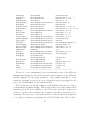
To summarize the tree and branch length information, type sumt relburnin =
yes burninfrac = 0.25. The sumt and sump commands each have separate burnin settings so it is necessary to give the burn-in here again. Most MrBayes settings
are persistent and need not be repeated every time a command is executed but the
settings are typically not shared across commands. To make sure the settings for
a particular command are correct, you can always use help <command> before
issuing the command.
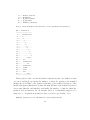
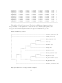
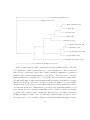
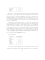
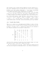
The sumt command will output, among other things, summary statistics for
the taxon bipartitions, a tree with clade credibility (posterior probability) values,
and a phylogram (if branch lengths have been saved). The output first gives a key
to each partition in the tree sample using dots for the taxa that are on one side
of the partition and stars for the taxa on the other side. For instance, the 14th
partition (ID 14) in the output below represents the clade Homo (taxon 3) and
Pan (taxon 4), since there are stars in the third and fourth positions and a dot in
all other positions.
List of taxa in bipartitions:
1
2
3
4
5
6
7
--------
Tarsius_syrichta
Lemur_catta
Homo_sapiens
Pan
Gorilla
Pongo
Hylobates
31
8
9
10
11
12
------
Macaca_fuscata
M_mulatta
M_fascicularis
M_sylvanus
Saimiri_sciureus
Key to taxon bipartitions (saved to file "primates.nex.parts"):
ID -- Partition
-----------------1 -- .***********
2 -- .*..........
3 -- ..*.........
4 -- ...*........
5 -- ....*.......
6 -- .....*......
7 -- ......*.....
8 -- .......*....
9 -- ........*...
10 -- .........*..
11 -- ..........*.
12 -- ...........*
13 -- .......****.
14 -- ..**........
15 -- ..**********
16 -- .......**...
17 -- ..*********.
18 -- ..*****.....
19 -- ..****......
20 -- ..***.......
21 -- .......***..
------------------
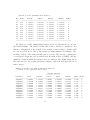
Then it gives a table over the informative bipartitions (the ones with more than
one taxon included), specifying the number of times the partition was sampled
(#obs), the probability of the partition (Probab.), the standard deviation of the
partition frequency (Sd(s)) across runs, the min and max of the standard deviation
across runs (Min(s) and Max(s)) and finally the number of runs in which the
partition was encountered. In our analysis, there is overwhelming support for a
single tree, so all partitions in this tree have a posterior probability of 1.0.
Summary statistics for informative taxon bipartitions
32
(saved to file "primates.nex.tstat"):
ID
#obs
Probab.
Sd(s)+
Min(s)
Max(s)
Nruns
---------------------------------------------------------------13
302
1.000000
0.000000
1.000000
1.000000
2
14
302
1.000000
0.000000
1.000000
1.000000
2
15
302
1.000000
0.000000
1.000000
1.000000
2
16
302
1.000000
0.000000
1.000000
1.000000
2
17
302
1.000000
0.000000
1.000000
1.000000
2
18
302
1.000000
0.000000
1.000000
1.000000
2
19
302
1.000000
0.000000
1.000000
1.000000
2
20
302
1.000000
0.000000
1.000000
1.000000
2
21
302
1.000000
0.000000
1.000000
1.000000
2
----------------------------------------------------------------
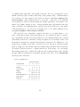
We then get a table summarizing branch and node parameters, in our case
the branch lengths. The indices in this table refer to the key to partitions. For
instance, length[14] is the length of the branch corresponding to partition ID
14. As we noted above, this is the branch grouping humans and chimps. The
meaning of most of the values in this table is obvious. The last two columns give
a convergence diagnostic, the Potential Scale Reduction Factor (PSRF), and the
numnber of runs in which the partition was encountered. The PSRF diagnostic is
the same used for the regular parameter samples, and it should approach 1.0 as
runs converge.
Summary statistics for branch and node parameters
(saved to file "primates.nex.vstat"):
95% HPD Interval
-------------------Parameter
Mean
Variance
Lower
Upper
Median
PSRF+ Nruns
-------------------------------------------------------------------------------------length[1]
0.486115
0.007159
0.349117
0.660632
0.477699
0.997
2
length[2]
0.335038
0.003829
0.222216
0.448005
0.331021
1.008
2
length[3]
0.050689
0.000114
0.033718
0.072349
0.049417
1.001
2
length[4]
0.060501
0.000144
0.039651
0.082690
0.060417
0.997
2
length[5]
0.057754
0.000183
0.031723
0.081064
0.056059
1.001
2
length[6]
0.143419
0.000537
0.100539
0.189667
0.140537
1.000
2
length[7]
0.172066
0.001072
0.112808
0.233264
0.172907
1.007
2
length[8]
0.016107
0.000031
0.005941
0.026377
0.015679
1.001
2
length[9]
0.023164
0.000045
0.011955
0.037226
0.022580
0.999
2
length[10]
0.056704
0.000147
0.033104
0.079370
0.056479
0.999
2
length[11]
0.069330
0.000366
0.029295
0.103081
0.070148
1.012
2
33
length[12]
0.433951
0.005270
0.305526
0.572054
0.426316
0.998
2
length[13]
0.248133
0.002680
0.148162
0.338245
0.243948
0.997
2
length[14]
0.029261
0.000142
0.008043
0.052766
0.028329
0.997
2
length[15]
0.273555
0.003600
0.163707
0.403779
0.268913
1.011
2
length[16]
0.035972
0.000125
0.016521
0.059122
0.035263
0.998
2
length[17]
0.118515
0.001761
0.044026
0.199364
0.119746
0.998
2
length[18]
0.124953
0.001162
0.052839
0.178939
0.122538
0.997
2
length[19]
0.057618
0.000424
0.017331
0.091541
0.057151
1.000
2
length[20]
0.082425
0.000486
0.051259
0.137057
0.080014
0.997
2
length[21]
0.049766
0.000398
0.018269
0.094330
0.047661
0.997
2
--------------------------------------------------------------------------------------
This table is followed by two trees. The clade credibility tree (upper tree) gives
the probability of each partition or clade in the tree, and the phylogram (lower
tree) gives the branch lengths measured in expected substitutions per site:
Clade credibility values:
/--------------------------------------------------------|
|--------------------------------------------------------|
|
/-------|
/--100--+
|
|
\-------|
/--100--+
|
|
\---------------|
/---100--+
+
|
\-----------------------|
/--100--+
|
|
\--------------------------------|
|
|
|
/-------|
/--100--+
/--100--+
|
|
|
|
\-------|
|
|
/--100--+
|
|
|
|
\---------------\--100--+
\-------100------+
|
\-----------------------|
\-------------------------------------------------
Phylogram (based on average branch lengths):
34
Tarsius_syrichta (1)
Lemur_catta (2)
Homo_sapiens (3)
Pan (4)
Gorilla (5)
Pongo (6)
Hylobates (7)
Macaca_fuscata (8)
M_mulatta (9)
M_fascicularis (10)
M_sylvanus (11)
Saimiri_sciureus (12)
/--------------------------------------- Tarsius_syrichta (1)
|
|--------------------------- Lemur_catta (2)
|
|
/---- Homo_sapiens (3)
|
/-+
|
| \----- Pan (4)
|
/------+
|
|
\---- Gorilla (5)
|
/---+
+
|
\------------ Pongo (6)
|
/--------+
|
|
\------------- Hylobates (7)
|
|
|
|
/-- Macaca_fuscata (8)
|
/---------+
/-+
|
|
|
| \-- M_mulatta (9)
|
|
|
/---+
|
|
|
|
\---- M_fascicularis (10)
\--------------------+
\-------------------+
|
\------ M_sylvanus (11)
|
\---------------------------------- Saimiri_sciureus (12)
|--------------| 0.200 expected changes per site
In the background, the sumt command creates five additional files. The first
is a .parts file, which contains the key to taxon bipartitions. The second and
third are the .tstat and .vstat files, which contain the summaries of partition
statistics and branch length statistics, respectively. The next is the .con file,
which includes the consensus trees. By default, the consensus tree with all the
relevant clade support values and branch length information is printed in a format
suitable for FigTree. Once the .con file is opened in FigTree, you can display
statistics such as the posterior probability and its associated standard deviation
on each clade in the tree. Alternatively, you can specify conformat=simple to get
the consenus trees in a simpler format that can be opened in most tree drawing
programs. The simple format contains two different trees, one with both branch
lengths and support values, and one with only branch lengths. Be sure to select
the appropriate one if you wish to display both branch lengths and support values.
35
The last file generated by the sumt command is the .trprobs file, which contains
the trees that were found during the MCMC search, sorted by posterior probability.
This allows you to examine the trees contained in various credible sets of trees.
For instance, the 95 % credible set contains the most probable trees up to an
accumulated posterior probability of 95 %. In our case, this file will only contain
one tree, but data sets with more topological uncertainty can produce .trprobs
files with a large number of trees.
3
Analyzing a Partitioned Data Set
MrBayes handles a wide variety of data types and models, as well as any mix of
these models. In this example we will look at how to set up a simple analysis of a
combined data set, consisting of data from four genes and morphology for 30 taxa
of gall wasps and outgroups. A similar approach can be used, e.g., to set up a
partitioned analysis of molecular data coming from different genes. The data set
for this tutorial is found in the file cynmix.nex.
3.1
Getting Mixed Data into MrBayes
First, open up the Nexus data file in a text editor. The DATA block of the
Nexus file should look familiar but there are some differences compared to the
primates.nex file in the format statement:
Format datatype=mixed(Standard:1-166,DNA:167-3246) interleave=yes gap=- missing=?;
First, the datatype is specified as datatype=mixed(Standard:1-166, DNA:167-3246).
This means that the matrix contains standard (morphology) characters in columns
1-166 and DNA characters in the remaining columns. The mixed datatype is an
extension to the Nexus standard. This extension was originated by MrBayes 3 and
may not be compatible with other phylogenetics programs.
Second, the matrix is interleaved. It is often convenient to specify mixed data
in interleaved format, with each block consisting of a natural subset of the matrix,
such as the morphological data or one of the gene regions.
36
3.2
Dividing the Data into Partitions
By default, MrBayes partitions the data according to data type. There are only
two data types in the matrix, so this model will include only a morphology (standard) and a DNA partition. To divide the DNA partition into gene regions, it
is convenient to first specify character sets. In principle, this can be done from
the command line but it is more convenient to do it in a MrBayes block in the
data file. With the MrBayes distribution, we added a file cynmix-run.nex with
a complete MrBayes block. For this section, we are going to create a command
block from scratch, but you can consult the cynmix-run.nex for reference.
In your favorite text editor, create a new file called cynmix-command.nex in
the same directory as the cynmix.nex file and add the following new MrBayes
block (note that each line must be terminated by a semicolon):
#NEXUS
begin mrbayes;
execute cynmix.nex;
charset morphology = 1-166;
charset COI = 167-1244;
charset EF1a = 1245-1611;
charset LWRh = 1612-2092;
charset 28S = 2093-3246;
The first line is required to comply with the nexus standard. With the execute
command, we load the data from the cynmix.nex file and the charset command
simply associates a name with a set of characters. For instance, the character set
COI is defined above to include characters 167 to 1244. The next step is to define
a partition of the data according to genes and morphology. This is accomplished
with the line (add it after the lines above):
partition favored = 5: morphology, COI, EF1a, LWRh, 28S;
The elements of the partition command are: (1) the name of the partitioning
scheme (favored); (2) an equal sign (=); (3) the number of character divisions in
the scheme (5); (4) a colon (:); and (5) a list of the characters in each division,
separated by commas. The list of characters can simply be an enumeration of
the character numbers (the above line is equivalent to partition favored = 5:
37
1-166, 167-1244, 1245-1611, 1612-2092, 2093-3246;) but it is often more
convenient to use predefined character sets like we did above. The final step is to
tell MrBayes that we want to work with this partitioning of the data instead of
the default partitioning. We do this using the set command:
set partition = favored;
Finally, we need to add anend statement to close the MrBayes block. The
entire file should now look like this:
#NEXUS
begin mrbayes;
execute cynmix.nex;
charset morphology = 1-166;
charset COI = 167-1244;
charset EF1a = 1245-1611;
charset LWRh = 1612-2092;
charset 28S = 2093-3246;
partition favored = 5: morphology, COI, EF1a, LWRh, 28S;
set partition = favored;
end;
When we read this block into MrBayes, we will get a partitioned model with
the first character division being morphology, the second division being the COI
gene, etc. Save the data file, exit your text editor, and finally launch MrBayes
and type execute cynmix-command.nex to read in your data and set up the
partitioning scheme. Note that this command causes MrBayes to read in the data
file because it contains the command execute cynmix.nex.
3.3
Specifying a Partitioned Model
Before starting to specify the partitioned model, it is useful to examine the default
model. Type showmodel and you should get this table as part of the output:
Active parameters:
Parameters
Partition(s)
1 2 3 4 5
38
-----------------------------Statefreq
1 2 2 2 2
Topology
3 3 3 3 3
Brlens
4 4 4 4 4
------------------------------
There is a lot of other useful information in the output of showmodel but this
table is the key to the partitioned model. We can see that there are five partitions
in the model and four active (free) parameters. There are two stationary state
frequency parameters, one for the morphological data (parameter 1) and one for
the DNA data (parameter 2). Then there is also a topology parameter (3) and a
set of branch length parameters (4). Both the topology and branch lengths are
the same for all partitions.
Now, assume we want a separate GTR + Γ + I model for each gene partition. All the parameters should be estimated separately for the individual genes.
Assume further that we want the overall evolutionary rate to be (potentially) different across partitions, and that we want to assume gamma-shaped rate variation
for the morphological data. We can obtain this model by using lset and prset
with the applyto mechanism, which allows us to apply the settings to specific partitions. For instance, to apply a GTR + Γ + I model to the molecular partitions,
we type lset applyto=(2,3,4,5) nst=6 rates=invgamma. This will produce
the following table when showmodel is invoked:
Active parameters:
Partition(s)
Parameters
1 2 3 4 5
-----------------------------Revmat
. 1 1 1 1
Statefreq
2 3 3 3 3
Shape
. 4 4 4 4
Pinvar
. 5 5 5 5
Topology
6 6 6 6 6
Brlens
7 7 7 7 7
------------------------------
As you can see, all molecular partitions now evolve under the correct model but
all parameters (statefreq, revmat, shape, pinvar) are shared across partitions.
39
To unlink them such that each partition has its own set of parameters, type:
unlink statefreq=(all) revmat=(all) shape=(all) pinvar=(all). Gamma-shaped
rate variation for the morphological data is enforced with lset applyto=(1)
rates=gamma. The trickiest part is to allow the overall rate to be different
across partitions. This is achieved using the ratepr parameter of the prset command. By default, ratepr is set to fixed, meaning that all partitions have the
same overall rate. By changing this to variable, the rates are allowed to vary under
a flat Dirichlet prior. To allow all our partitions to evolve under different rates,
type prset applyto=(all) ratepr=variable.
The model is now essentially complete but there is one final thing to consider. Typically morphological data matrices do not include all types of characters. Specifically, morphological data matrices do not usually include any constant
(invariable) characters. Sometimes, autapomorphies are not included either, and
the matrix is restricted to parsimony-informative characters. For MrBayes to calculate the probability of the data correctly, we need to inform it of this ascertainment (coding) bias. By default, MrBayes assumes that standard data sets include
all variable characters but no constant characters. If necessary, one can change
this setting using lset coding. We will leave the coding setting at the default,
though, which is variable for standard (morphology) data. Now, showmodel
should produce this table:
Active parameters:
Partition(s)
Parameters
1 2 3 4 5
-----------------------------Revmat
. 1 2 3 4
Statefreq
5 6 7 8 9
Shape
10 11 12 13 14
Pinvar
. 15 16 17 18
Ratemultiplier 19 19 19 19 19
Topology
20 20 20 20 20
Brlens
21 21 21 21 21
------------------------------
40
3.4
Running the Analysis
When the model has been completely specified, we can proceed with the analysis essentially as described above in the tutorial for the primates.nex data set.
However, in the case of the cynmix.nex dataset, the analysis will have to be run
longer before it converges.
When looking at the parameter samples from a partitioned analysis, it is useful
to know that the names of the parameters are followed by the character division
(partition) number in curly braces. For instance, pi(A){3} is the stationary frequency of nucleotide A in character division 3, which is the EF1a division in the
above analysis.
In this section we have used a separate Nexus file for the MrBayes block.
Although one can add this command block to the data file itself, there are several
advantages to keeping the commands and the data blocks separate. For example,
one can create a set of different analyses with different parameters in separate
command files and submit all those files to a job scheduling system on a computer
cluster. It is important to remember, though, that MrBayes uses the name of the
file containing the character matrix as the default for all output files. Thus, if
you run all your analyses in the same directory, results from different analyses will
overwrite each other.
To change this behavior, include the command mcmcp filename=<filename>;
in each of your run files, just before issuing the mcmc command, using a different file
name for each run file. For instance, if you wish to name the output files from one
analysis using the root analysis1, you use the line mcmcp filename=analysis;.
The files will then be named analysis1.run1.t, analysis1.run2.t, etc. An alternative approach is to run each analysis in a separate directory, in which case
the naming of the output files will not be an issue.
3.5
Some Practical Advice
As you continue exploring Bayesian phylogenetic inference, you may find the following tips helpful:
1. The convergence diagnostics provided by MrBayes are quite powerful but
they certainly do not exhaust the possibilities. Several programs will read MrBayes
output files and will provide you with a number of additional ways in which you can
41
examine the output from your analysis. Two of the most popular tools are Tracer
and AWTY. Among other things, they provide nice graphical representations of
the output from MCMC analyses.
2. If you are anxious to get results quickly, you can try running without
Metropolis coupling (heated chains). This will save a large amount of computational time at the risk of having to start over if you have difficulties getting
convergence. Turn off heating by setting the mcmc option nchains to 1 and switch
it on by setting nchains to a value larger than 1.
3. If you are using heated chains, try to make sure that the acceptance rates
of swaps between adjacent chains are in the approximate range of 10 to 70 %. The
acceptance rates are printed to the .mcmc file and to screen at the end of the run.
The latter output contains a table that looks like this (you find the critical values
in a different format in the .mcmc file):
1
2
3
4
1
2
3
4
-------------------------|
0.53 0.26 0.12
| 3347
0.55 0.31
| 3295 3337
0.53
| 3332 3396 3293
It is the values just above the diagonal, {0.53, 0.55, 0.53} in this case, that you
should focus on. If the acceptance rates are lower than 10 %, decrease the temperature constant (mcmc temp=<value>); if the acceptance rates are higher than
70 %, increase it. Acceptance rates outside the optimal range do not invalidate
the results from your analysis, they only mean that you could make your analysis
more efficient.
4. If you run multiple simultaneous analyses or use Metropolis coupling and
have access to a machine with several processors or processor cores, or if you
have access to a computer cluster, you can speed up your analyses considerably
by running MrBayes in parallel under MPI. See the MrBayes web site for more
information about this.
5. If you are using automatic optimization of proposal tuning parameters,
and your runs are reasonably long so that MrBayes has sufficient time to find the
best settings, you should not have to adjust proposal tuning parameters manually. However, if you have difficulties getting convergence, you can try selecting a
42
different mix of topology moves than the one used by default. For instance, the
random SPR move tends to do well on some data sets but it is switched off by
default because, in general, it is less efficient than the default moves. You can add
and remove topology moves, or change the frequency with which they are used, by
adjusting their relative proposal probabilities using the propset command. Use
showmoves allavailable=yes first to see a list of all the available moves.
For more information and tips, turn to the MrBayes web site (http://mrbayes.net),
Fredrik’s MrBayes resources page (http://www.sc.fsu.edu/~fronquis/mrbayes),
the MrBayes home on SourceForge (http://www.sf.net/projects/mrbayes) and
the MrBayes users email list.
4
Evolutionary Models Implemented in MrBayes
3
MrBayes implements a wide variety of evolutionary models for nucleotide, amino
acid, restriction site (binary), and standard discrete data. In addition, there are
several different ways of modeling the process generating phylogenetic trees. An
overview of all the models is given in diagrammatic form in the Appendix. Here,
we provide a brief description of each model with some comments on their implementation in MrBayes and advice on how you can apply them successfully to your
data.
4.1
Nucleotide Models
MrBayes implements a large number of DNA substitution models. These models
are of three different structures. The ”4by4 ” models are the usual simple models
of nucleotide evolution. The “Doublet ” model is intended for stem regions of
ribosomal DNA, where nucleotides evolve in pairs. Finally, the “Codon ” models
group the nucleotides in triplets and model evolution based on these. The type
of nucleotide model is set in MrBayes with lset nucmodel ; for instance, if you
want to use the doublet model, the command is lset nucmodel=doublet . The
default setting is 4by4 .
43
4.1.1
Simple Nucleotide Models
There has been more work based on the simple four by four nucleotide models
than on any other type of evolutionary model for molecular data. MrBayes 3
implements three main types of models; you select among those by setting the
number of substitution types using lset nst to 1, 2, or 6. The widely used
General Time Reversible (GTR) model has six substitution types (lset nst=6 ),
one for each pair of nucleotides. The instantaneous rate matrix for the GTR model
is (note that we order the rows and columns alphabetically - A, C, G, T - unlike
some other authors)


[A]

Q=
[C]

[G]
[T ]

[A]
[C]
[G]
[T ]

−
πC rAC πG rAG πT rAT 

πA rAC
−
πG rCG πT rCT 


πA rAG πC rCG
−
πT rGT 
πA rAT πC rCT πG rGT
−
The GTR model (Tavare, 1986) has four stationary state frequencies (πA , πC , πG , πT )
and six rate parameters (rAC , rAG , rAT , rCG , rCT , rGT ). In total, there are eight free
parameters, since one of the stationary state frequencies and one of the substitution
rates are determined by the others. By default, MrBayes uses a “flat” Dirichlet
distribution (with all distribution parameters set to 1) as the prior for both the
stationary state frequencies and the substitution rates. This is a reasonable uninformative prior that should work well for most analyses.
During the analysis, both the stationary state frequencies and substitution
rates are estimated. If you want to fix the stationary state frequencies or substitution rates, you can do that by using the prset command. For instance,
assume that we want to fix the stationary state frequencies to be equal, converting the GTR model to the so-called SYM model. This is achieved by prset
statefreqpr=fixed(0.25,0.25,0.25, 0.25) or, more conveniently, prset statefreqpr=fixed(e
44
. The substitution rate matrix now

[A]

[A]
−


Q = [C] 0.25rAC

[G] 0.25rAG
[T ] 0.25rAT
becomes

[C]
[G]
[T ]

0.25rAC 0.25rAG 0.25rAT 

−
0.25rCG 0.25rCT 


0.25rCG
−
0.25rGT 
0.25rCT 0.25rGT
−
and the stationary state frequencies are no longer estimated during the analysis.
Similarly, it is possible to fix the substitution rates of the GTR model using
prset revmatpr=fixed . Assume, for instance, that we want to fix the substitution rates to be (rAC = 0.11, rAG = 0.22, rAT = 0.12, rCG = 0.14, rCT = 0.35, rGT =
0.06). Then the correct statement would be prset revmatpr=fixed(0.11,0.22,0.12,0.14,0.35,
0.06) . Note the order of the rates. The substitution rates can be given either
as percentages of the rate sum, as here, or they can be scaled to the rGT rate.
The former representation is the Dirichlet parameterization used internally by
MrBayes. By default, MrBayes reports substitution rates in the Dirichlet format
but you can request conversion of sampled rates to the scaled format using the
report command if you prefer this representation. One disadvantage with the
scaled format is that the posterior distribution tends to be strongly skewed such
that the arithmetic mean of the sampled values is considerably higher than the
mode and the median. Therefore, consider using the median instead of the mean
when reporting a posterior distribution sampled in the scaled format.
Before using the GTR model for some of your data, we recommend that you
make sure there are at least a few possible substitutions of each type. For instance,
if there is not a single GT substitution in your data, it will be difficult to estimate
the GT substitution rate. In such cases, you should consider either the HKY model
(nst=2 ) or the F81 model (nst=1 ) instead of the GTR model. The HKY model
(Hasegawa, Kishino and Yano, 1985) has different rates for transitions (rti ) and
45
transversions (rtv ):


[A]

Q=
[C]

[G]
[T ]

[A]
[C]
[G]
[T ]

−
πC rtv πG rti πT rtv 

πA rtv
−
πG rtv πT rti 


πA rti πC rtv
−
πT rtv 
πA rtv πC rti πG rtv
−
The HKY model is often parameterized in terms of the ratio between the
transition and transversion rates, κ = rti /rtv , and this is the default format used
by MrBayes when reporting samples from the posterior distribution. Internally,
however, MrBayes uses the Dirichlet parameterization in which the transition and
transversion rates are expressed as percentages of the (unscaled) rate sum. If you
prefer, you can have MrBayes report the sampled values using the Dirichlet format
instead of the ratio format by using the command report tratio=dirichlet .
The caveats described above for the GTscaled substitution rates also apply to the
transition / transversion rate ratio. In the .p files, the ratio will be referred to
as kappa and the transition and transversion rate proportions will be referred to
as ti and tv . The setting of the report tratio option will determine whether
you will see a single kappa column or the two ti and tv columns.
As with the GTR model, you can fix both the stationary state frequencies and
the transition / transversion rate ratio of the HKY model. If you fix the stationary
state frequencies to be equal, you will get the K2P model (Kimura, 1980).
Finally, MrBayes implements the F81 model (Felsenstein, 1981), which assumes
that all substitution rates are equal but stationary state frequencies are not, that
is


[A] [C] [G] [T ]


[A] − πC πG πT 



Q=
[C] πA − πG πT 


[G] πA πC − πT 
[T ] πA πC πG −
If the stationary state frequencies are fixed to be equal using prset statefreqpr=fixed(equal)
, you will get the simplest of all nucleotide substitution models, the JC model
(Jukes and Cantor, 1969).
46
A large number of other subsets of the GTR model are often used in Maximum
Likelihood inference. Why do we not allow more substitution model types in
MrBayes? One of the most important advantages of the Bayesian approach is
that it allows you to integrate out uncertainty concerning the model parameters
you have little information about. Thus, Bayesian inference is relatively robust
to slight over-parameterization of your model. In addition, the MCMC sampling
procedure is typically efficient in dealing with complex multi-parametric models.
For these reasons, it is less important in the Bayesian context to find the simplest
possible model that can reasonably represent your data. If you use a modeltesting procedure and it suggests a four by four nucleotide model not implemented
in MrBayes, then you should obtain good results using the next more complex
model available in the program.
4.1.2
The Doublet Model
The doublet model of MrBayes is intended for stem regions of ribosomal sequences,
where nucleotides pair with each other to form doublets. The nucleotide pairing
results in strong correlation of substitutions across sites - when there is a substitution at one site it is typically accompanied by a compensatory substitution at
the paired site. If the correlation between paired sites is not accounted for, parametric statistical methods will overestimate the confidence we should have in the
best tree(s). Incidentally, the same is true for parsimony and the non-parametric
bootstrap.
There are various ways to model the evolution of nucleotide doublets. One
method is to focus on the common doublets, A-T and C-G in particular. MrBayes
uses a more complex model, originally formulated by Schoniger and von Haeseler
(1994), where all doublets are taken into account. The central idea in this model
is that one common doublet is converted into another through a two-step process.
In the first step, one of the nucleotides is substituted with another according to a
standard four by four model of nucleotide change. In the second step, the matching
nucleotide is changed according to the same standard four by four model. Thus,
in this model there is no momentary change from one doublet to another doublet;
this always occurs through an intermediate, rare doublet.
Assume that we are using a GTR model for the single nucleotide substitutions,
47
that i and j are two different doublets, that dij is the minimum number of nucleotides that must be changed when going between i and j, and that mn is the
pair of nucleotides that change when going between i and j when dij = 1. Then
the elements qij of the instantaneous rate matrix Q of the doublet model can be
expressed as follows
(
0
if dij > 1
qij =
πj rmin
if dij = 1
for the case when i differs from j; the diagonal elements (i = j) are determined, as
usual, to balance the rows in the instantaneous rate matrix to sum to zero. This
gives the instantaneous rate matrix (only 7 rows and columns out of 16 shown):


 [AA]

[AC]


[AG]

Q=
 [AT ]

[CA]

[CC]

 ···

[T T ]
[AA]
−
πAA rAC
πAA rAG
πAA rAT
πAA rAC
0
···
0
[AC]
[AG]
πAC rAC πAG rAG
−
πAG rCG
πAC rCG
−
πAC rCT πAG rGT
0
0
πAC rAC
0
···
···
0
0
[AT ]
[CA]
[CC]
πAT rAT πCA rAC
0
πAT rCT
0
πCC rAC
πAT rGT
0
0
−
0
0
0
−
πCC rAC
0
πCA rAC
−
···
···
···
πAT rAT
0
0

···
[T T ]

···
0 

···
0 


···
0 

· · · πT T rAT 


···
0 

···
0 

···
··· 

···
−
Instead of using the GTR model, we could of course have used the HKY or F81
model, resulting in obvious modifications of the rmn values. Use lset nst to
change among those options; for instance, use lset nst=6 to choose the GTR
model. The default model is the F81 model (lset nst=1 ).
Before the doublet model can be used, it is necessary to specify all the nucleotide pairs in the alignment. This is done using the pairs command, most
conveniently in a MrBayes block in a data file. For instance, pairs 1:10, 2:9;
would pair nucleotide 1 with 10 and 2 with 9. See the kim.nex data file for an
example of an analysis using the doublet model.
4.1.3
Codon Models
The codon models implemented in MrBayes are based on the first formulations of
such models (Goldman and Yang, 1994; Muse and Gaut, 1994). The approach is
48
similar to that used in the doublet model. A codon can change to another only
through steps of one nucleotide change at a time. These steps are modeled using
a standard four by four nucleotide model. There is one additional complication
though: some nucleotide changes are synonymous while others lead to changes in
amino acids and thus may be subject to selection (a factor modifying the substitution rate). Assume that i and j are different codons, that a(i) is the amino acid
coded for by codon i, that dij is the minimum number of nucleotide changes involved in changing between them, and that ω is the ratio of the non-synonymous to
the synonymous substitution rate. The off-diagonal elements of the instantaneous
rate matrix can now be defined as


if dij >1
 0
qij =
πj rmin
if dij =1 and a(i) = a(j)


πj rmin ω
if dij =1 and a(i) 6= a(j)
with the diagonal elements being defined to balance the rows of the instantaneous
rate matrix, as usual. The single-nucleotide substitution rates can be modeled
using the GTR, the F81, or the JC model, as before. Use lset nst to change
among those options; for instance, use lset nst=6 to choose the GTR model.
The default model is the F81 model (lset nst=1 ).
Invoking the codon model is easy; just make sure that the aligned DNA or RNA
sequences start with a nucleotide in codon position 1 and that they end with a
nucleotide in codon position 3. Also, make sure that the sequences do not contain
any stop codons. To figure out whether a codon is a stop codon and whether a
particular single-nucleotide change involves an amino acid change, MrBayes uses
one of several genetic codes. By default, MrBayes uses the universal code but you
can select other codes by using the lset code command. Note that the codon
models are computationally demanding. Whereas the computations for the simple
four by four models need to deal with only 16 Q-matrix and transition probability
elements (4x4), the codon model computations need to process more than 3,600
Q-matrix and transition probability elements resulting in these runs being roughly
200 times slower. The codon models also require much more memory than the
four by four models, about 16 times as much.
The simplest codon model, described above, assumes that all amino acid sites
are subject to the same level of selection (the same ω factor). However, MrBayes
49
also implements models accommodating variation in selection across sites. This
allows you to detect positively selected amino-acid sites using a full hierarchical
Bayes analysis (that is, an analysis that does not fix tree topology, branch lengths
or any substitution model parameters but instead integrates out uncertainty in all
these factors).
The ω variation models work much like the model accommodating rate variation across sites according to a gamma distribution. The likelihood of each site is
calculated under several different ω values and then the values are summed to give
the site likelihood. A difference is that the stationary frequency of each omega
category is estimated, instead of being fixed as in the case of the gamma distribution. There are two variants implemented in MrBayes, and they are invoked
using the lset omegavar option. In the Ny98 model (Nielsen and Yang, 1998),
there are three classes with potentially different ω values: 0 < ω1 < 1, ω2 = 1, and
ω3 > 1. The M3 model also has three classes of ω values but these values are less
constrained in that they only have to be ordered ω1 < ω2 < ω3 . If, for instance,
you would like to invoke the M3 model, use the command lset omegavar=M3 .
When you use a model with variation in selection pressure across sites, you
probably want to infer the positively selected sites. If you select report possel=yes
before you start your analysis, MrBayes will calculate the probability of each site
being in a positively selected omega class. For the M3 model, for instance, the
likelihood of the site is calculated under each of the three categories, taking the
category frequencies into account, and then the likelihoods are summed to yield
the total likelihood of the site. Finally, the proportion of this sum originating from
categories that are positively selected (those that have an ω value larger than 1);
this is the posterior probability of the site being positively selected.
Once the probabilities of each site being positively selected are printed to file,
they can be summarized using the standard sump command. When interpreting
the output from the Ny98 model, it is helpful to know that pi(-), pi(N) and
pi(+) are the frequencies of the negatively selected, neutral and positively selected categories, respectively, and omega(-), omega(N) and omega(+) are the
corresponding ω values. The M3 model parameters are instead labeled pi(1),
pi(2) and pi(3) for the category frequencies and omega(1), omega(2) and
omega(3) for the ω values. The probability of a codon being positively selected
is labeled by the site numbers in the original alignment. Thus pr+(16,17,18) is
50
the probability of the codon corresponding to the original nucleotide alignment
sites 16, 17, and 18 being in a positively selected omega category.
4.2
Amino-acid Models
MrBayes implements a large number of amino-acid models. They fall in two distinct categories: the fixed-rate models and the variable-rate models. The former
have both the stationary state frequencies and the substitution rates fixed, whereas
one or both of these are estimated in the latter.
4.2.1
Fixed Rate Models
The Poisson model (Bishop and Friday, 1987) is the simplest of the fixed rate
models. It assumes equal stationary state frequencies and equal substitution rates;
thus, it is analogous to the JC model for nucleotide characters. The rest of the
fixed-rate models have unequal but fixed stationary state frequencies and substitution rates reflecting estimates of protein evolution based on some large training
set of proteins. These models include the Dayhof f model (Dayhoff, Schwartz
and Orcutt, 1978), the M trev model (Adachi and Hasegawa, 1996), the M tmam
model (Cao et al., 1998; Yang, Nielsen, and Hasegawa, 1998), the W AG model
(Wheland and Goldman, 2001), the Rtrev model (Dimmic et al., 2002), the Cprev
model (Adachi et al., 2000), the V t model (Muller and Vingron, 2000) and the
Blosum62 model (Henikoff and Henikoff, 1992). Each model is appropriate for a
particular type of proteins. For instance, if you are analyzing mammal mitochondrial proteins, you might want to use the Mtmam model. Invoke that model by
typing prset aamodelpr=fixed(mtmam) .
4.2.2
Estimating the Fixed Rate Model
MrBayes allows a convenient way of estimating the fixed-rate model for your amino
acid data instead of specifying it prior to the analysis. If you choose this option,
MrBayes will allow the MCMC sampler to explore all of the fixed-rate models listed
above, including the Poisson model, by regularly proposing new models. When
the MCMC procedure has converged, each model will contribute to your results in
proportion to its posterior probability. For instance, if you are analyzing mammal
51
mitochondrial proteins, it is likely that the Mtmam model will contribute most to
the posterior distribution but it is possible that some other models, for instance
the Mtrev model, will contribute significantly too. A nice feature of the MCMC
model estimation is that the extra computational cost is negligible.
To allow so-called model jumping between fixed-rate amino acid models, simply
set the prior for the amino acid model to mixed, prset aamodelpr=mixed , prior
to analysis. During the run, MrBayes will print the index of the current model to
the .p file(s) in the aamodel column. The indices of the models are as follows: 0
= Poisson, 1 = Jones, 2 = Dayhoff, 3 = Mtrev, 4 = Mtmam, 5 = Wag, 6 = Rtrev,
7 = Cprev, 8 = Vt, 9 = Blosum. When you use the sump command, you will get
a table with the names of the amino acid models and their posterior probabilities.
4.2.3
Variable Rate Models
There are two variable-rate models implemented in MrBayes for amino acid data.
The Equalin model is a “glorified” F81 model in that it allows the stationary state
frequencies of all amino acids to be different but assumes the same substitution
rate. Thus, the instantaneous rate matrix for this model is


 [A]

 [R]


[N ]

Q=
[D]

 [C]

 [Q]

· · ·

[V ]
[A]
−
πA
πA
πA
πA
πA
···
πA
[R]
πR
−
πR
πR
πR
πR
···
πR
[N ]
πN
πN
−
πN
πN
πN
···
πN
[D]
πD
πD
πD
−
πD
πD
···
πD
[C]
πC
πC
πC
πC
−
πC
···
πC
[Q]
πQ
πQ
πQ
πQ
πQ
−
···
πQ

· · · [V ]

· · · πV 

· · · πV 


· · · πV 

· · · πV 


· · · πV 

· · · πV 

· · · · · ·

··· −
and it has 19 free parameters (20 stationary state frequencies minus one because
the frequencies sum to 1) that will be estimated from data.
The other variable-rate model is the “glorified” GTR model, which allows all
stationary state frequencies and substitution rates to vary. Thus, the instantaneous
52
rate matrix for this model is

[A]
[R]

 [A]
−
πR rAR

 [R] π r
−
A AR


[N ] πA rAN πR rRN

Q=
[D] πA rAD πR rRD

 [C] πA rAC πR rRC

 [Q] πA rAQ πR rRG

· · ·
···
···

[V ] πA rAV πR rRV
[N ]
πN rAN
πN rRN
−
πN rN D
πN rN C
πN rN Q
···
πN rN V
[D]
πD rAD
πD rRD
πD rN D
−
πD rDC
πD rDQ
···
πD rDV
[C]
πC rAC
πC rRC
πC rN C
πC rDC
−
πC rCQ
···
πC rCV
[Q]
πQ rAQ
πQ rRQ
πQ r N Q
πQ rDQ
πQ rCQ
−
···
πQ rQV
···
···
···
···
···
···
···
···
···

[V ]

πV rAV 

πV rRV 


πV rN V 

πV rDV 


πV rCV 

πV rQV 

··· 

−
and the model has 19 free stationary state frequency parameters and 189 free
substitution rate parameters. The Bayesian MCMC approach is good at handling
uncertainty in multiparameter models, so the GTR model may be used successfully
with moderate-size data sets, but the model is so parameter-rich that you need
a fairly sizable data set to be able to estimate all parameters with reasonable
precision.
The GT R model can be used to express a user-derived fixed rate model other
than those already implemented in MrBayes. Simply use the prset command to
fix the stationary state frequencies and substitution rates of the GTR model to
the desired values. You need to set two options, prset aarevmatpr=fixed(<190
comma-separated values>) and prset statefreqpr=fixed(<20 comma-separated
values>) . Once the values are fixed prior to analysis, the MCMC procedure will
not change them and they will remain the same throughout the analysis.
4.2.4
Restriction Site (Binary) Model
MrBayes implements a simple F81-like model for restriction sites and other binary
data. The instantaneous rate matrix for this model is simply


[0] [1]


Q = [0] − π1 
[1] π0 −
53
Any asymmetry in the rate of 0 to 1 and 1 to 0 transitions is expressed in terms of
the stationary state frequencies. Thus, if the stationary frequencies are π0 = 0.25
and π1 = 0.75, then the rate of 0 to 1 transitions is 3 times as high as the rate of
transitions in the other direction (π1 /π0 = 3).
A problem with some binary data sets, notably restriction sites, is that there is
an ascertainment (coding) bias such that certain characters will always be missing
from the observed data. It is impossible, for instance, to detect restriction sites that
are absent in all of the studied taxa. MrBayes corrects for this bias by calculating
likelihoods conditional on the unobservable characters being absent (Felsenstein,
1992). The ascertainment (coding) bias is selected using lset coding . There
are five options: (1) there is no bias, all types of characters could, in principle, be
observed (lset coding=all ); (2) characters that are absent (state 0) in all taxa
cannot be observed (lset coding= noabsencesites ); (3) characters that are
present (state 1) in all taxa cannot be observed (lset coding=nopresencesites
); (4) characters that are constant (either state 0 or 1) in all taxa cannot be
observed (lset coding=variable ); and (5) only characters that are parsimonyinformative have been scored (lset coding=informative ). For restriction sites
it is typically true that all-absence sites cannot be observed, so the correct coding
bias option is noabsencesites .
The binary model is useful for a number of character types other than restriction sites. For instance, the model can be used for gap characters. The presence
and absence of gaps must be coded consistently for all characters; let us assume
here that absence of a gap is coded as 0 and presence as 1. Since the detection of
gaps is typically contingent on observing some sequence length variation, neither
all-absence nor all-presence characters can be observed. Thus, the correct ascertainment bias for gap characters is variable . The parameters π0 and π1 would
represent the rate at which insertions and deletions occur, respectively (assuming
that state 0 denotes absence of a gap).
The binary model can also be used for ecological, morphological, or other binary
characters of arbitrary origin. However, if the binary model is applied to more than
one character, then there is an implicit assumption that the state labels are not
arbitrary for those characters. That is, the 0 state in one character must somehow
be comparable to the 0 state in the others. For instance, 0 could mean absence
(or presence) of a particular type of feature, such as a wing vein, a restriction site,
54
or a gap in a DNA sequence. It is not appropriate to apply the default binary
model to a set of characters where the state labels are arbitrary, as is true of most
morphological characters. Thus, we can possibly estimate the rate of loss versus
gain of wing veins over a set of consistently coded wing venation characters, but
we cannot compare the rate of loss of antennal articles to the rate at which a
yellow patch evolves into a green patch. If state labels are truly arbitrary, then
the stationary state frequencies of the binary model must be fixed to be equal, such
that the estimation of model parameters becomes independent of the labeling of
character states. An alternative is to consider the standard model, which provides
more sophisticated ways of dealing with arbitrary state labels.
When is the correction for ascertainment bias important? This is strongly
dependent on the size of the tree (the sum of the branch lengths on the tree). The
larger the tree, the less important the correction for ascertainment bias becomes.
In our experience, when there are more than 20-30 taxa, even the most severe bias
(only informative characters observed) is associated with an insignificant correction
of the likelihood values.
4.2.5
Standard Discrete (Morphology) Model
The model used by MrBayes for standard discrete data is based on the ideas
originally presented by Lewis (2001). Essentially, the model is analogous to a JC
model except that it has a variable number of states, from 2 to 10. For instance,
a three-state standard character would be evolving according to the instantaneous
rate matrix


[0] [1] [2]
[0] − 1 1 


Q=

[1] 1 − 1 
[2] 1 1 −
Because all rates are the same, we can maintain the essential property of standard characters, namely that state labels are arbitrary. Thus, the standard model
assures that you will get the same results regardless of the way in which you label
the states.
In morphology-based parsimony analyses, one sometimes distinguishes between
55
ordered and unordered characters. In ordered characters, evolution between some
states is assumed to go through intermediate states. MrBayes implements a
stochastic model for such characters. For a three-state character assumed to be
ordered (by convention in the sequence 0-1-2), the instantaneous rate matrix is


[0] [1] [2]
[0] − 1 0 


Q=

[1] 1 − 1 
[2] 0 1 −
Note that the instantaneous rate of going between the two end states is 0, that
is, a transition from 0 to 2 or from 2 to 0 has to go through state 1. By default,
MrBayes treats all standard characters as unordered. To change this, use the
ctype command. For instance, if you want to treat characters 3 and 4 as ordered
you need to include the statement ctype ordered: 3 4; in your MrBayes block
(or enter it using the command line, if you prefer).
The number of states of each standard character is determined by MrBayes
simply by looking at the state codes in your matrix. Thus, a three-state model will
be used for a three-state character and a six-state model for a six-state character.
MrBayes does not check that all state codess are used, it simply finds the largest
state code in the matrix for each character. Thus, make sure that you use the
state codes 0, 1, and 2 for a three-state character and state codes 0, 1, 2, 3, 4, and
5 for a six-state character.
Because state labels are arbitrary in the standard model, we cannot estimate
unequal stationary state frequencies or substitution rates (recall that the stationary
state frequencies are an important factor in determining the latter). However, it
is still possible to allow the state frequencies (rates) to vary over sites according to
some appropriate distribution. MrBayes uses a symmetric Dirichlet distribution
for this purpose. For binary data, the analogy of the Dirichlet distribution is
called the beta distribution; MrBayes uses Dirichlet and beta interchangeably for
the distribution depending on context. The approach is similar to the one used to
allow rate variation across sites according to a gamma distribution: we calculate
the likelihood of a site assuming different discrete categories of asymmetry and
then we sum the values to obtain the site likelihood.
The symmetric Dirichlet distribution has one parameter that determines its
56
shape, just like the alpha parameter determines the shape of the gamma distribution. The larger the parameter of the symmetric Dirichlet, the less transition rate
(stationary frequency) asymmetry there is across sites. By default, the parameter
is fixed to infinity (prset symdirihyperpr=fixed(infinity) ); this corresponds
to the standard assumption of no transition rate asymmetry across sites: the rate
of going from 0 to 1 is equal to the rate of going from 1 to 0 for all characters.
The prior is called a hyperprior because it concerns a distribution that controls
the distributions of other model parameters (stationary state frequencies in this
case). If you want to allow transition rate (stationary frequency) asymmetry in
standard data, then simply select another (hyper)prior. For instance, you can fix
the parameter to 1.0, which would result in a uniform prior on the proportions of
the state frequencies.
In practice, MrBayes uses a discrete approximation of the Dirichlet distribution
for binary characters; five categories are used by default (change this with lset
nbetacat ). For instance, assume that we fix the hyperprior to 1.0 and then
evaluate the likelihood of one binary character using five discrete beta categories.
MrBayes would then calculate the likelihood of the character assuming that the
stationary state frequencies of the two states were 0.1:0.9, 0.3:0.7, 0.5:0.5, 0.7:0.3
and 0.1:0.9. The five category likelihoods would then be multiplied by 0.20 (there
is a probability of 0.20 of being in each of the categories) and then summed up
to give the total likelihood of the character. For multistate characters, MrBayes
does not use the discrete approximation; instead, it uses the MCMC procedure to
explore different stationary state frequency proportions.
4.3
Parsimony Model
MrBayes implements an incredibly parameter-rich model, first described by Tuffley
and Steel (1997). It orders trees in terms of their maximum likelihood in the same
way as the parsimony method would order them in terms of their parsimony score;
hence we call it the parsimony model. The model is also referred to as the NoCommon-Mechanism model because it treats each branch length for each character
as a separate, completely independent parameter. In principle, a Bayesian MCMC
analysis using the parsimony model should integrate out the branch lengths but
MrBayes 3 uses a simpler approach, in which the branch lengths are fixed to their
57
maximum likelihood values (infinity if there is a change on the branch and zero
otherwise). This type of approach, where some parameters are fixed prior to the
Bayesian analysis according to some non-Bayesian estimate, is typically referred
to as an empirical Bayes method. Future versions of MrBayes may implement the
true (hierarchical) Bayesian approach to the parsimony model but we expect the
results to be very similar under both approaches.
The parsimony model is much less parsimonious with respect to parameters
than any other model implemented in MrBayes. Consider, for instance, an analysis
of 1,000 characters and 100 taxa. The parsimony model would have about 200,000
free parameters (200 branches times 1,000 characters). A more typical GTR +
+ I model would have only little more than 200 parameters, about 1,000 times
fewer parameters. In this sense, the standard stochastic models are much more
parsimonious than the parsimony model. Several problems are associated with
the excessive number of parameters. Statistical inconcistency is perhaps the best
known of these but, more fundamentally, a model like the parsimony model does
not offer much in terms of generalities that can be inferred about the evolutionary
process.
The Goldman (1993) model is another example of a parameter-rich stochastic
model that orders trees in the same way as the parsimony method. In this model,
the branch lengths are the same but the ancestral states are estimated for all characters and all nodes in the tree. For an analysis of 100 taxa and 1,000 characters,
this results in approximately 100,000 free parameters. The Goldman model is actually very similar to the No- Common-Mechanism model; it makes little difference
if the character-specific and treesection- specific parameters are introduced at the
nodes or at the branches. The Goldman model is not implemented in MrBayes.
We would like to emphasize that we do not recommend the use of the parsimony
model. We have included it in MrBayes only to allow users to explore its properties
and contrast it with the other models implemented in the program. The parsimony
model is not the default model used for standard (morphological) data in MrBayes.
The default standard data model is described above and is similar to the models
used for nucleotide and amino acid data. By default, MrBayes does not use the
parsimony model at all; you have to invoke it using lset parsmodel=yes .
58
4.4
Rate Variation Across Sites
By default, MrBayes assumes that all characters evolve at the same rate (measured
in expected changes per site over the tree). There are four ways in which you can
allow rate variation across sites. The simplest method is to assume that rates vary
over sites according to a gamma distribution (Yang, 1993). The gamma model can
be combined with spatial autocorrelation between the rates at adjacent sites, the
autocorrelated gamma model. A completely different approach to rate variation
across sites is to allow a proportion of sites to be invariable. This model can be
combined with the gamma model but not with the autocorrelated gamma model.
Finally, it is possible to divide characters into groups evolving at different rates,
the partitioned or site specific rate model.
4.4.1
Gamma-distributed Rate Model
The commonly used model of gamma-shaped rate variation across sites is invoked
using lset rates=gamma . The shape of the gamma distribution is determined
by the socalled α (alpha) parameter. When this parameter is small (below 1),
the distribution takes on an L-shaped form with a few sites evolving rapidly while
most sites are conserved. Conversely, when α is above 1 the distribution becomes
similar to a normal distribution with less and less variation in rates across sites as
α becomes larger.
In practice, the gamma distribution is approximated using a small number of
discrete rate categories (Yang, 1994). By default, four rate categories are used; you
can change this setting by using lset ngammacat . For instance, if you want to
use eight discrete rate categories the appropriate command is lset ngammacat=8
. The computational complexity is proportional to the number of categories used.
An analysis with four discrete gamma categories is four times as slow as an analysis
with no rate variation across sites and twice as fast as one with eight categories.
The shape parameter (α) of the gamma distribution is similar to the shape
parameter of the Dirichlet distribution of stationary state frequencies used for
standard data (see above) in that it controls the distribution of another model
parameter (the site rates). Therefore, the prior probability distribution used for
the shape parameter can be referred to as a hyperprior. The default prior used in
MrBayes is a uniform distribution on the interval (0.05,50). The sampled values of
59
the shape parameter are found under the column heading alpha in the .p file(s).
4.4.2
Autocorrelated Gamma Model
In this model, rates vary across sites according to an autocorrelated gamma model
where the rate at each site depends to some extent on the rates at adjacent sites
(Yang, 1995). The spatial autocorrelation is measured by the ρ (rho) parameter,
which ranges from -1 (negative autocorrelation, that is, adjacent sites tend to have
wildly different rates) to 1 (adjacent sites have very similar rates). The default
prior probability for rho is a uniform distribution covering the entire interval (-1,1).
In the worst case, a small symmetric tree, the extra computational complexity
incurred by invoking the auto correlated gamma model instead of the gamma
model is comparable to a doubling of the number of taxa in the analysis. In more
typical cases, moderate to large data sets, the additional computational cost is
negligible and equivalent to adding a single taxon. As with the gamma model,
the autocorrelated gamma distribution is approximated with a number of discrete
rate categories determined by lset ngammacat .
As described by Yang (1995), protein-coding sequences tend to have a threeposition offset in their autocorrelation. That is, the first codon position sites tend
to have rates that are correlated with the adjacent first-position sites, secondposition site rates are correlated with adjacent second-position rates, etc. You
can take this effect into account by partitioning your sites into the three codon
positions and then applying a separate autocorrelated gamma model to each of
the categories.
You might want to invoke an autocorrelated gamma model with the same
correlation coefficient for a dataset consisting of several concatenated genes. If
so, it is necessary to inform MrBayes about the break points between different
genes. Otherwise, the rates at the first site of each gene except the first one will
be erroneously compared to the rates at the last site in the preceding gene. The
command databreaks is provided for this purpose. For instance, if there are
only two genes in your data set, the first with 960 sites, you would specify the
break between them with the statement databreaks 960 . Note that you specify
the break by giving the last sequence site before the break. The databreaks
command is only needed when you invoke a single autocorrelated gamma model
60
for a multigene dataset. The databreaks command cannot be used to partition
a data set.
4.4.3
Proportion of Invariable Sites
A completely different approach to rate variation is to allow a proportion of sites to
be invariable. This model is invoked using lset rates=propinv . The proportion
of invariable sites is referred to as pinvar; it can vary from 0 (no invariable sites)
to 1 (all sites are invariable). The default prior is a uniform distribution on the
interval (0,1); change it using prset pinvarpr .
The proportion of invariable sites model can be combined with the gamma
model using lset rates=invgamma . Although this model is slightly better than
the simple gamma model for many data sets, it sometimes results in a bimodal or
ridge-like posterior probability distribution. In particular, it is not uncommon to
see two peaks in the posterior, one with a low proportion of invariable sites and
significant rate variation in the gamma distribution (low alpha value) and the other
with a high proportion of invariable sites and moderate amounts of rate variation
in the gamma distribution (moderately high alpha value). If you have a posterior
of this kind, you should not be surprised if Metropolis-coupling results in rapid
(instantaneous) shifts from one mode to the other during the stationary phase
of the analysis. The reason for this is that different chains are likely to explore
different peaks in the posterior, and successful swapping involving the cold chain is
likely to result in mode-jumping. Also, you should consider presenting the entire
distribution of the sampled alpha and pinvar parameters since simple point
estimates of each parameter would be misleading.
4.4.4
Partitioned (Site Specific) Rate Model
For protein-coding nucleotide sequences, a site-specific rate model is often used,
allowing each codon position (first, second and third codon position sites) to have
its own rate. This results in a model with three rates, two of which are free to
vary (since the average rate is 1.0 by definition). More generally, we might have
different character divisions (separate genes, morphology, etc) which potentially
evolve at very different rates.
In MrBayes 3, we provide a general mechanism for setting up these models
61
based on partitioning the data set and then unlinking parameters across the partitions. Assume for instance that we want to set up a site specific rate model for
a data set with one sequence. We first set up the codon site partitioning scheme
using the following lines in a MrBayes block:
charset pos1 = 1-.\3;
charset pos2 = 2-.\3;
charset pos3 = 3-.\3;
partition by_codon = 3: pos1, pos2, pos3;
set partition = by_codon;
The character sets are first defined using the dot sign (.) to mark the last
character in the data set and the \3 sequence to include every third character
in the specified range. Then a partitioning scheme called by codon is defined
using the previously named character sets. Finally, the partitioning scheme called
by codon is invoked using the set command.
When we process these commands in MrBayes using the execute command,
the characters are divided into three sets corresponding to the codon positions.
By default, however, all model parameters including the rate will be shared across
partitions. To allow the rates to differ across partitions, we need to change the prior
for rates using prset . Specifically, prset ratepr=variable invokes partitionspecific rates. The partition-specific rate parameter is referred to as ratemult ,
and the individual rates are labeled m{1} , m{2} , etc for the rate (multiplier) of
character division 1, 2, etc. See below for more information on how to set up
partitioned models.
4.4.5
Inferring Site Rates
When you are allowing rate variation across sites, you may be interested in inferring the rates at each individual site. By default, the site rates are not sampled
during a MCMC run. You need to request the sampling of these values using
report siterates=yes . The rates will be referred to as r(<site number>) .
For instance, r(45) is the inferred rate at site (character) 45 of your data set.
62
4.5
Rate Variation Across the Tree: The Covarion Model
For both nucleotide sequence and amino-acid data, MrBayes allows rates to change
across the tree under a covarion-like model (Tuffley and Steel, 1998; Huelsenbeck,
2002; see also Galtier, 2001). Specifically, the covarion-like model assumes that a
site is either “on” or “off”. When it is on, it evolves under a standard four-by-four
nucleotide or 20 by 20 amino acid model but when it is off, it does not change at
all. The switching between on and off states is controlled by two rate parameters,
s01 (from off to on) and s10 (from on to off). The instantaneous rate matrix of
the nucleotide variant (also referred to as the covariotide model), assuming a GTR
model for the on state, is


[Aof f ]

 [C ]
 of f

[Gof f ]

Q=
 [Tof f ]

 [Aon ]

 [Con ]

 [G ]
 on
[Ton ]

[Aof f ] [Cof f ] [Gof f ] [Tof f ] [Aon ]
[Con ]
[Gon ]
[Ton ]

−
0
0
0
s01
0
0
0 

0
−
0
0
0
s01
0
0 


0
0
−
0
0
0
s01
0 

0
0
0
−
0
0
0
s01 


s10
0
0
0
−
πC rAC k πG rAG k πT rAT k 

0
s10
0
0
πA rAC k
−
πG rCG k πT rCT k 

0
0
s10
0
πA rAG k πC rCG k
−
πT rGT k 

0
0
0
s10 πA rAT k πC rCT k πG rGT k
−
where k is a scaling constant determined by the proportion of time the sites
spend in the on state. The matrix can be simplified into
"
#
R1 R2
Q=
R3 kR4
where each R element is a four by four matrix: R1 contains the rates in the
off state (all rates are 0), R2 and R3 describe the switching process (the diagonal
elements are either s01 or s10 ), and R4 is the chosen model for the evolution in the
on state.
The covarion-like model can be described as a general case of the proportion of
invariable sites model (Huelsenbeck, 2002). As the switching rates go to zero, the
proportion of these rates represented by the switch to the off state (s1 0) becomes
63
identical to the proportion of invariable sites. When the switching rates are zero,
there is no exchange between the on and off states and the characters in the off
state remain off throughout the tree; in other words, they are invariable sites.
Note that the covarion-like model implemented in MrBayes differs from the
original covarion model in that sites switch completely independently of each other
between the on and off states. To invoke the covarion-like model, simply use lset
covarion=yes and then choose the desired nucleotide or amino acid model using
the other lset and the prset options. The covarion-like model can be combined
with the gamma model of rate variation across sites.
4.6
Topology and Branch Length Models
The topology and branch length models in MrBayes are set using the prset
topologypr options, which deal with the tree topology prior, and the prset
brlenspr options, which deal with the branch lengths.
4.6.1
Unconstrained and Constrained Topology
There are two choices for the prior probability distribution on topology: uniform
or constrained. By default, topologies are not constrained in the prior (prset
topologypr=uniform ), resulting in equal prior probability being associated with
all possible labeled trees (unless a different topology prior is induced by the branch
length model, see below). There are two instances in which you might want to
constrain the topology: (1) when you want to contrast a hypothesis of monophyly
for a group with the more general hypothesis with no topological constraints; and
(2) when you want to infer ancestral states for a particular node in the tree. In
both cases, you specify the constraint(s) first by listing the taxa that should form
a monophyletic group. For instance, if you wanted to constrain taxa 4, 5 and 6 to
be monophyletic, you would use
constraint my_constraint -1 = 4 5 6;
This defines a constraint called my constraint forcing taxa 4, 5 and 6 to form a
monophyletic group in all trees that are sampled from the chain. In future versions
of MrBayes, the value following the name of the constraint (-1 here), will give the
relative probability of trees having the constrained partition. A negative number
64
will force the constraint to always be present in the sampled trees; a positive
number will specify how many times more likely the trees with the constraint are
compared to the trees not having it. In version 3.1, however, MrBayes ignores this
value and always treats the constraint as absolute. When you define constraints,
make sure that you have the outgroup selected correctly. By default, MrBayes
uses the first taxon in the data matrix as the outgroup. You can change this by
using the outgroup command. For instance, if you want taxon number 7 called
My taxon to be the outgroup, either use outgroup 7 or outgroup My taxon .
MrBayes 3.1 only allows a single taxon as the outgroup.
Before the constraints take effect, you have to invoke them by using prset
topologypr=constraints(<comma-separated list of constraints>) . For instance, to enforce the constraint my constraint defined above, use prset topologypr=constraints(
.
4.6.2
Non-clock (Standard) Trees
If you do not want to enforce a molecular clock, you choose an unconstrained
branch length prior. Actually, you do not have to do anything because unconstrained branch lengths are the default. You can associate unconstrained branch
lengths with either a uniform prior from 0 to some arbitrary value or an exponential prior. The default is an exponential distribution with parameter 10
(Exponential(10) ); it has an expectation of 0.1 (= 1/10) but (in principle) it
allows branch lengths to vary from 0 to infinity. The exponential distribution
apparently puts a lot more probability on short branches than on long branches.
However, because transition (substitution) probabilities change rapidly at small
branch lengths but only very slowly at long branch lengths, the exponential prior
is actually closer to an uninformative prior than the uniform distribution. We
advise against using a uniform prior on branch lengths because of the large prior
probability it puts on long branches and their close-to-random substitution probabilities.
To change the prior on unconstrained branch lengths you use prset brlenspr
. For instance, assume you wanted to use an exponential prior with parameter 1 instead of the default prior. This prior is set by typing prset brlenspr=unconstrained:
exponential(1) .
65
4.6.3
Strict Clock Trees
MrBayes implements three strict clock models: the simple (uniform) model, the
birthdeath model, and the coalescence model. The birth-death model and coalescence models both have additional parameters describing the tree-generating
process, whereas the simple model does not.
In the birth − death model (see Yang and Rannala, 1997, for a Bayesian implementation), trees are generated according to a birth-death model with a speciation
and an extinction rate. The model, as implemented in MrBayes, can also be associated with a sampling probability of terminal lineages. The priors for these three
parameters are set using the speciationpr, extinctionpr, and sampleprob
parameters of the prset command.
In the coalescence model, the tree generating process is looked at from the
opposite perspective, backward in time. Instead of lineages branching, this model
sees them as coalescing into fewer and fewer ancestral lineages. This process occurs
at a rate determined by the θ (theta) parameter; it is also affected by the ploidy
of the data (haploid or diploid). The prior for the theta parameter is set using
prset thetapr . The ploidy level is set using lset ploidy .
The simple clock model is invoked by prset brlenspr=clock:uniform . There
is only one additional parameter in the simple clock model, namely the total tree
height. The prior for this parameter is set by prset treeheightpr . The default
prior is an exponential distribution with parameter 1.0 (Exponential(1.0) ).
4.6.4
Relaxed Clock Trees
Relaxed clock models and functions for dating are not implemented in MrBayes
3.1. According to current plans, they will be available in version 3.2.
4.6.5
Partitioned Models
MrBayes provides great flexibility in setting up partitioned models. By default,
the characters are divided into partitions based on the data type. If there is only
one data type in the matrix, then all characters will be in a single partition. The
default partitioning scheme is called default . For information on how to set up
a file with mixed data types, see the example file cynmix.nex and the tutorial in
section 3 of this manual.
66
You can easily set up partitioning schemes that divide the characters up further
than the default partition does using the partition command. The most convenient way of partitioning data is to define character sets first using the charset
command. For instance, assume that you have concatenated nucleotide sequences
from three genes in your data set of length 1962, 1050, and 2082 sites, respectively.
Then you create character sets for those three genes using
charset gene1 = 1-1962;
charset gene2 = 1963-3012;
charset gene3 = 3013-.;
in a MrBayes block. Note the use of the dot (.) as a synonym of the last
site. You can also use the backslash n sequence to include every nth character
in the preceding range of characters (see the description of the site specific rate
model above). Once the character sets are defined, the partitioning scheme based
on the genes is defined with the partition command and selected using the set
command:
partition by_gene = 3: gene1, gene2, gene3;
set partition=by_gene;
Here, by gene is the name we chose for the partitioning scheme. The name is
followed by an equal sign, the number of partitions, and then a comma-separated
list of characters to include in each partition. Note that MrBayes requires the
partitioning scheme to include all characters. Say, for instance, that you wanted
to run an analysis with only gene 1 and gene 2. Then define a two-partition scheme
and exclude the characters represented by gene 3:
partition gene1&2 = 2: gene1, gene2 gene3;
exclude gene3;
set partition=gene1&2;
If the only purpose of the partition gene1&2 is to allow exclusion of gene 3,
then gene 3 can of course be included in either of the two partitions before being
excluded.
Once the partitions have been correctly set up, MrBayes allows you to set
models for individual partitions using the lset applyto and prset applyto
67
mechanism. For instance, assume that we have two partitions, a standard data
partition (partition 1) and a nucleotide partition (partition 2), and want to apply a GTR model to the nucleotide data, gamma-shaped rate variation to both
partitions, and allow the partition rates to be different. Then we would use the
commands
lset applyto=(2) nst=6;
lset applyto=(all) rates=gamma;
prset applyto=(all) ratepr=variable;
By default, all model parameters that are identical and have the same prior
probability distribution associated with them, are linked across partitions (they are
assumed to be one and the same parameter). To unlink parameters, use the unlink
command. For instance, assume that we want to unlink the shape parameter across
the partitions discussed above (after all, why should the standard data and the
molecular data have the same distribution of rates across sites?). This would be
achieved using
unlink shape=(all);
If you unlink parameters by mistake, they can be linked again using the link
command. All of the commands mentioned above and given as they would appear
in a MrBayes block in a Nexus file can of course be entered from the command line
as well (without the trailing semicolon). However, it is often more convenient to
have them in either your data file or in a separate Nexus file that you process after
you have read in your data. MrBayes will keep the data set in memory until you
read in a new data block, so you can have your different MrBayes blocks pertaining
to the same data file distributed over as many separate Nexus files as you like.
We recommend that, before you run your analysis, you check the current model
settings using the showmodel command. This command will list all the active parameters and how they are linked across partitions, as well as the priors associated
with each parameter.
Finally, we want to give you a warning. Even though MrBayes allows you
to easily set up extremely complex and parameter-rich models, and the Bayesian
MCMC approach is good at handling such models, think carefully about the parameters you introduce in your model. There should be at least some reasonable
68
chance of estimating the parameters based on your data. For instance, a common
mistake is to use a separate GTR model for a partition with so few substitutions
that there is not a single observation for several rate categories. Making sure there
are at least some observations allowing you to estimate each parameter is good
practice. Over-parameterized models often result in problems with convergence in
addition to the excessive variance seen in the parameter estimates.
4.7
Ancestral State Reconstruction
MrBayes allows you to infer ancestral states at ancestral nodes using the full
hierarchical Bayesian approach (integrating out uncertainty concerning topology
and other model parameters). The basic approach is described by Huelsenbeck
and Bollback (2001) as well as in a recent review (Ronquist, 2004). You first need
to constrain the node you want to infer ancestral states for using a constraint
definition and the topologypr=constraints(...) command as described above
for constrained topology models. Then ancestral state reconstruction is requested
using report ancstates=yes.
The probability of each state will be printed to the .p file(s) under the heading
p(<state code>)character number . For instance, the probability of an A at site
215 in a nucleotide data set would be found under the heading p(A){215} . If you
constrain several nodes in your data set, the node number will be given as well. If
you had constrained two nodes, the probabilities of the above character would be
distinguished as p(A){215@1} and p(A){215@2} . However, if you are interested
in inferring ancestral states at two or more different nodes, we recommend running
separate analyses, each constraining a single node. The reason is that when you
focus on one node, you probably want to integrate over uncertainty in the rest of
the tree, including the potential uncertainty concerning the presence of the other
node(s).
Often, there is interest in mapping only one or a few characters onto trees
inferred using largely other types of data. For instance, a behavioral or ecological trait may be mapped onto trees based on molecular data. To do this type of
analysis in MrBayes, you would set up a mixed data set including both the character to be mapped and the data used to infer the phylogeny, with the character
to be mapped in a separate data partition. How to do this is explained in the
69
tutorial given in section 3 of this manual as well as in the description of partitioned models above. Typically, you also want to assume that the evolutionary
rate for the mapped character is proportional to that of the other data (rather
than identical). This is achieved by setting up a partitioned rate model using
prset ratepr=variable . Then you need to set up a constraint for the node of
interest, as described above. Finally, you request that ancestral states are inferred
for the partition with the mapped character (there is no need to wade through
ancestral state probabilities for the other partition(s)). For instance, if the character to be mapped is in partition 2, request ancestral state sampling using prset
applyto=(2) ancstates=yes. Now only the ancestral states for the character
of interest will be printed to the .p file(s). The sampled values can be summarized
as usual with the sump command.
5
Frequently Asked Questions
How do I cite the program?
If you want to cite the program, we suggest you use the two papers published
in Bioinformatics (Huelsenbeck and Ronquist, 2003; Ronquist and Huelsenbeck,
2005). If you are using the MPI version of the program, you may also want to cite
Altekar et al. (2004).
How do I run MrBayes in batch mode?
When you become more familiar with MrBayes, you will undoubtedly want
to run it in batch mode instead of typing all commands at the prompt. This is
done by adding a MRBAYES block to a Nexus file, either the same file containing
the DATA block or a separate Nexus file. The MRBAYES block simply contains
the commands as you would have given them from the command line, with the
difference that each command line is ended with a semi-colon. For instance, a MRBAYES block that performs three single-run analyses of the data set primates.nex
under the GTR + model and stores each result in a separate file is given below:
begin mrbayes;
set autoclose=yes nowarn=yes;
execute primates.nex;
lset nst=6 rates=gamma;
mcmc nruns=1 ngen=10000 samplefreq=10 file=primates.nex1;
70
mcmc file=primates.nex2;
mcmc file=primates.nex3;
end;
Since this file contains the execute command, it must be in a file separate
from the primates.nex file. You start the analysis simply by typing execute
<filename> , where filename is the name of the file containing the MRBAYES
block. The set command is needed to change the behavior of MrBayes such that it
is appropriate for batch mode. When autoclose = yes , MrBayes will finish the
MCMC analysis without asking you whether you want to add more generations.
When nowarn = yes , MrBayes will overwrite existing files without warning you,
so make sure that your batch file does not inadvertently cause the deletion of
previous result files that should be saved for future reference.
The UNIX version of MrBayes can execute batch files in the background from
the command prompt. Just type mb <file> > log.txt & at the UNIX prompt,
where <file> is the name of your Nexus batch file, to have MrBayes run in
the background, logging its output to the file log.txt . If you want MrBayes to
process more than one file, just list the files one after the other with space between
them, before the output redirection sign (¿). When MrBayes is run in this way, it
will quit automatically when it has processed all files; it will also terminate with
an error signal if it encounters an error.
Alternatively, the UNIX version of MrBayes can also be run in batch mode
using input redirection. For that you need a text file containing the commands
exactly as you would have typed them from the command line. For instance,
assume that your data set is in primates.nex and that you want to perform the
same analyses specified above. Then type mb < batch.txt > log.txt & with
the batch.txt file containing this text:
set autoclose=yes nowarn=yes
execute primates.nex
lset nst=6 rates=gamma
mcmc ngen=10000 savebrlens=yes file=primates.nex1
mcmc file=primates.nex2
mcmc file=primates.nex3
quit
The quit command forces MrBayes to terminate. With previous versions of
71
MrBayes we have had problems with infinite loops when the quit command is not
included at the end of the file. This problem should have been solved in version
3.1.
How are gaps and missing characters treated?
MrBayes uses the same method as most maximum likelihood programs: it
treats gaps and missing characters as missing data. Thus, gaps and missing characters will not contribute any phylogenetic information. There is no way in which
you can treat gaps as a fifth state in MrBayes (but see below for information on
how you can use gap information in your analysis).
How do I use gap information in my analysis?
Often, insertion and deletion events contain phylogenetically useful information. Although MrBayes 3 is not able to do statistical multiple sequence alignment,
treating the insertion-deletion process under a realistic stochastic model, there is
nevertheless a way of using some of the information in the indel events in your
MrBayes analysis: Code the indel events as binary characters (presence/absence
of the gap) and include them as a separate binary (restriction) data partition in
your analysis. See more information on this possibility in the section on the binary
model in this manual.
What do I do when it is difficult to get convergence?
There are several things you can do to improve the efficiency of your analysis.
The simplest is to just increase the length of the run. However, the computational
cost of doing so may be prohibitive. A better way is then to try improving the
mixing behavior of the chain. First, examine the acceptance rates of the proposal
mechanisms used in your analysis (output at the end of the run). The Metropolis
proposals used by MrBayes work best when their acceptance rate is neither too low
nor too high. A rough guide is to try to get them within the range of 10 % to 70 %.
Rates outside this range are not necessarily a big problem but they typically mean
that the analysis is inefficient. If the rate is too high, you can make the proposal
bolder by changing tuning parameters (see Appendix) using the props command.
Be warned, however, that changing tuning parameters of proposals and proposal
probabilities may destroy any hope of getting convergence. For instance, you need
at least one move changing each parameter in your model.
The next step is to examine the heating parameters if you are using Metropoliscoupled MCMC. If acceptance rates for the swaps between adjacent chains (the
72
values close to the diagonal in the swap statistics matrix) are low, then it might be
a good idea to decrease the temperature to make the cold and heated chains more
similar to each other so that they can change states more easily. The efficiency of
the Metropolis coupling can also be improved by increasing the number of parallel
chain.
A good way of improving convergence is to start the analysis from a good tree
instead of starting it from a randomly chosen tree. First define a good tree, with
or without branch lengths, using the command usertree . Then start the chains
from this tree using mcmcp startingtree=user . A disadvantage with starting
the analysis from a good tree is that it is more difficult to detect problems with
convergence using independent runs. A compromise is to start each chain from a
slightly perturbed version of a good tree. MrBayes can introduce random perturbations of a starting tree; this is requested using mcmcp nperts=<integer value>
.
How do I run MrBayes in parallel?
See section 7 of this manual.
The likelihood values first increase and then drop. What is the problem?
Several users have observed that likelihood values can sometimes increase in
the early phase of a run and then decrease to a stable value; one user referred to
the phenomenon as burn-out. Actually, this type of behavior can be seen with
certain types of data sets and models and is part of the normal burn-in. However,
it does indicate a problem with the model. Typically, the problem is due to overparameterization, a poor prior, or a combination of these factors.
In MrBayes, the starting value for most parameters is an arbitrarily chosen
value that is likely to be close to the maximum likelihood estimate (MLE) of
the parameter. The MLE value typically also corresponds to the mode (peak) in
the posterior probability distribution. In most cases, you expect the bulk of the
probability mass in the posterior probability distribution to be in the region close
to the MLE. However, it is possible that there is a region in parameter space with
only moderate height (lower likelihood values) but considerably larger probability
mass than the MLE region. It is like comparing the mass of a tower to the mass of
a huge office complex. Even if the tower is considerably higher, its mass is going
to be only a fraction of the mass of the office complex.
A typical situation in which this can occur is if you: (1) use a uniform prior
73
on branch lengths, which puts considerable prior probability on long branches; (2)
have data that are relatively uninformative about branch lengths; and (3) have
a model, such as the gamma model, with a low but not insignificant probability
associated with long branches for weak data. In such cases, the MLE region at
short branch lengths can have considerably smaller probability mass than the less
likely but much larger region at longer branch lengths.
A typical situation in which this can occur is if you: (1) use a uniform prior
on branch lengths, which puts considerable prior probability on long branches; (2)
have data that are relatively uninformative about branch lengths; and (3) have
a model, such as the gamma model, with a low but not insignificant probability
associated with long branches for weak data. In such cases, the MLE region at
short branch lengths can have considerably smaller probability mass than the less
likely but much larger region at longer branch lengths.
Unless you feed MrBayes with your own starting tree, the run will start with all
branch lengths set to 0.1. This is close to the MLE region, and in the early phase
of the run you will see the likelihood values climb as the topology is improved
by branch rearrangements while the branch lengths remain small. Eventually,
however, the long branch length region will attract the chain through its high
probability mass and you will see the branch lengths increase and the likelihood
values decrease to a stable region.
There are basically two ways of fixing the burn-out problem. One is to change
your priors so that they put more probability in the MLE region. An obvious
step is to change a uniform prior on branch lengths to an exponential prior; as
explained above in the section on branch length priors, an exponential prior is more
uninformative than the uniform prior anyway. The other possibility is to simplify
your model. For instance, assume equal rates over sites instead of a gamma model,
or choose a substitution model with fewer free parameters.
How can I test models using Bayes factors? The Bayesian approach provides
a convenient way of comparing models through the calculation of Bayes factors,
which can be interpreted as indicators of the strength of the evidence in favor of
the best of two models. The Bayes factor values are typically interpreted according
to recommendations developed by Kass and Raftery (1995).
Unlike a hierarchical likelihood ratio test, the models compared with Bayes
factors need not be hierarchically nested. A Bayes factor is calculated simply
74
as the ratio of the marginal likelihoods of the two models being compared. The
logarithm of the Bayes factor is the difference in the logarithms of the marginal
model likelihoods.
The marginal likelihood of a model is difficult to estimate accurately but a
rough estimate may be obtained easily as the harmonic mean of the likelihood
values of the MCMC samples (Newton and Raftery, 1994). MrBayes calculates
this estimator when you summarize your samples with the command sump . In the
output from the sump command, you will find the following table (it might look
a little different depending on how many simultaneous runs you have performed;
this table is for two runs):
Estimated marginal likelihoods for runs sampled in files
"replicase.nex.run1.p", "replicase.nex.run2.p", etc:
(Use the harmonic mean for Bayes factor comparisons of models)
Run
Arithmetic mean
Harmonic mean
-------------------------------------1
-5883.41
-5892.10
2
-5883.82
-5892.81
-------------------------------------TOTAL -5883.60
-5892.52
--------------------------------------
For instance, assume we want to compare a GTR model with an HKY model.
Then simply run two separate analyses, one under each model, and estimate the
logarithm of the marginal likelihoods for the two models (using only samples from
the stationary phase of the runs). Then simply take the difference between the
logarithms of the harmonic means and find the corresponding interpretation in the
table of Kass and Raftery (1995; to use this table, you actually have to calculate
twice the difference in the logarithm of the model likelihoods). The same approach
can be used to compare any pair of models you are interested in. For instance,
one model might have a group constrained to be monophyletic while the other
is unconstrained, or one model can have gammashaped rate variation while the
other assumes equal rates across sites. As stated above, models need not be
hierarchically nested. An interesting property of the Bayes factor comparisons
is that it can favor either the more complex model or the simpler model, so they
75
need not be corrected for the number of parameters in the models being compared.
Additional discussion of Bayesian model testing, with several examples, is found
in Nylander et al. (2004).
Can I do model-jumping in MrBayes?
Bayesian MCMC model jumping provides a convenient alternative to model
selection prior to the analysis. In model jumping, the MCMC sampler explores
different models and weights the results according to the posterior probability of
each model.
The only model jumping implemented in MrBayes 3 is the estimation of fixedrate amino-acid substitution models (see the section on those models in this manual). General model jumping across models of different dimensionality will be
implemented in version 4 of MrBayes.
ModelTest suggests a model for my data. How do I implement it in MrBayes?
A model selection procedure, such as that implemented in ModelTest and MrModelTest, often suggests a quite specific model for your analysis, including estimates of all parameters. This suggestion is often based on several simplifications;
for instance, you might have fixed the topology when comparing models and you
might have used a small set of the possible models. In the Bayesian approach, there
is only a moderate computational penalty associated with estimating parameters
rather than fixing them prior to analysis. The Bayesian approach is typically also
good at handling multi-parameter models. Therefore, we recommend that you take
the general type of model suggested by your model selection method and then estimate all of the parameters in that model in MrBayes. If the suggested model is not
implemented in MrBayes, use the next more complex model available in the program. If, for some reason, you feel that you really need to fix model parameters in
MrBayes to specific values, you can do that using prset <parameter prior name>
= fixed (<value or commaseparated values>) . For instance, if you want to
fix the shape parameter of the gamma model to 0.12, use prset shapepr=fixed(0.05)
.
How many data partitions can I have in MrBayes?
MrBayes 3 allows 150 partitions. If you need more partitions, simply change
the variable MAX NUM DIVS in the source file mb.h and recompile the program.
Does MrBayes run faster on a dual-processor machine?
No. The Windows and Mac versions of MrBayes 3.1 are not multithreaded
76
so they will not take advantage of more than one processor on a single machine.
However, you should be able to run two copies of MrBayes without noticeable
decrease in performance on a dual-processor machine (provided you have enough
RAM for both analyses).
How much memory is required?
You can calculate the amount of memory needed to store the conditional likelihoods for an analysis roughly as 2 * (# taxa) * (# states in the Q matrix) *
(# gamma categories) * 4 bytes (for the single-precision float version of the code;
double the memory requirement for the double-precision code). The program will
need slightly more memory for various book-keeping purposes but the bulk of the
memory required for an analysis is typically occupied by the conditional likelihoods.
How do I fix the tree topology during an analysis?
In principle, one can fix a tree topology by specifying constraints for all of
the nodes in the tree. However, we do not recommend doing this because it is
computationally very inefficient. A better way is to set the proposal probability
of all topology moves to 0 using the props command. Then you need to switch
on one proposal that changes branch lengths but not topology by increasing its
proposal probability from 0 to some reasonable positive value (like 5). The node
slider is, in our experience, the best of these proposals.
6
Differences Between Version 2 and Version 3
We have discontinued the development of version 2 of MrBayes and recommend
all users to switch over to version 3. With the release of version 3.1, virtually all
models implemented in version 2 are available in version 3 (plus many more). The
only exception is the time-irreversible model of nucleotide evolution, which is still
not implemented in version 3. If you are interested in seeing this model reappear,
let us know.
An important difference between versions 2 and 3 is found in the way models
are defined. MrBayes 3 by default estimates most parameters, there is no need
to specify estimate for any parameter. Some things that were previously set using
lset are now set using prset . This is true for the amino acid model and for
the site specific rates (see section 4 of this manual for more information on the
77
site specific rate model in version 3). Thus, site-specifc rates, for instance, can no
longer be invoked using rates=sitespec .
In more detail, the changes are as follows, with emphasis on the features in
version 2 that are implemented differently in version 3 (commands and options in
version 2 listed alphabetically):
calibration . Calibration of clock and relaxed-clock trees is not (yet) implemented in MrBayes 3.
constraint . The format of the constraint now includes a probability value
(constraint <name> <probability> = <list of taxa>) . The probability value
is ignored by version 3.1 of the program but it must be included in the constraint
definition. The probability value will be used by future versions of the program.
lset aamodel . The amino-acid model is now set using prset aamodelpr .
lset ancfile . Ancestral states are now written to the .p file(s).
lset basefreq . Whether this parameters is estimated or fixed to a particular
value in version 3 is controlled by setting the prior with prset statefreqpr . By
default, all parameters are estimated. There is no basefreq option in the lset
command of version 3 of MrBayes.
lset clock . Whether the tree is a clock or a non-clock tree is now set using
prset brlenspr .
lset enforcecal . Calibrations are not implemented (yet) in MrBayes 3.
lset enforcecodon . The type of nucleotide model is now set using lset
nucmodel=4by4/doublet/codon .
lset enforcecon . Now set using prset topologypr = constraints (<list of constraints
.
lset inferanc . Now set using report ancstates .
lset inferpossel . Now set using ¡tt¿report possel¡tt¿.
lset inferrates . This is now set with report siterates .
lset ncat (number of categories used to approximate the gamma distribution
of site rates). Now set using lset ngammacat to distinguish it from nbetacat
(the number of categories used to approximate the beta distribution of rate /
stationary state asymmetry across sites in the standard model).
lset nonrevmat . Time-irreversible models are not implemented in MrBayes
3.
lset omega . Whether this parameters is estimated or fixed to a particular
78
value in version 3 is controlled by setting the prior with prset omegapr . By
default, all parameters are estimated. There is no omega option in the lset
command of version 3 of MrBayes.
lset rates . The site specific rate models (sitespec , ssgamma , ssadgamma
) are now set using the more general partitioning model. See section 3 of this
manual as well as the discussion of partition models in section 4.
lset revmat . Whether this parameters is estimated or fixed to a particular
value in version 3 is controlled by setting the prior with prset revmatpr . By
default, all parameters are estimated. There is no revmat option in the lset
command of version 3 of MrBayes.
lset seqerror . The model of sequencing error is no longer implemented
in MrBayes 3. The model typically results in small corrections in partition support values but it conflicts with important algorithmic short-cuts implemented in
version 3.
lset shape . Whether this parameters is estimated or fixed to a particular
value in version 3 is controlled by setting the prior with prset shapepr . By default, all parameters are estimated. There is no shape option in the lset command
of version 3 of MrBayes.
lset sitepartition . The partition of sites is now set using set partition
.
lset tratio . Whether this parameters is estimated or fixed to a particular
value in version 3 is controlled by setting the prior with prset tratiopr . By
default, all parameters are estimated. There is no tratio option in the lset
command of version 3 of MrBayes.
prset basefreqpr . Now set using prset statefreqpr .
prset brlenpr . Now set using prset brlenspr . The options are now more
complicated as well, since the prior includes information both about the general
type of the branch lengths (clock, non-clock) and the specific shape of the prior
(for example, uniform or exponential).
prset siteratepr . Now set using prset ratepr . The options are fixed or
variable (Dirichlet). The parameters of the Dirichlet can be set to reflect various
types of prior information concerning the site rates.
prset qmatpr . Now set using prset revmatpr and prset aarevmatpr for
nucleotide and amino-acid substitution rates, respectively.
79
set . This command only controlled the autoclose option in MrBayes 2. In
version 3 it controls a number of different things, including the currently selected
partition.
shownodes . This command is no longer included in MrBayes 3. Use showtree
to display the user tree.
7
7.1
Advanced Topics
Compiling MrBayes
Compiling the MrBayes executable from the source code can be done on several
different compilers targeting all the common operating systems: Macintosh, Windows, and Unix. The easiest way to build MrBayes is to use the included configure
script and with a make tool for the Makefile this script generates. One can also
compile MrBayes with the Metroworks Codewarrior and Microsoft Visual Studio
suites.
Some performance gain can be achieved by using different compiler optimization flags. Keep in mind, that not all options are safe to use. A number of optimization methods might give a slowdown instead of a speedup and some options
relax numerical assumptions, leading to a program that might produce incorrect
results. When you want to file a bug report, make sure that you compiled the
program with the default options.
7.1.1
Compiling with GNU Make and configure
The configure script that is distributed with the MrBayes source code examines
your build environment for appropriate compiler flags and program settings. In
most cases you can run this script (./configure ) without any arguments and it
will produce a Makefile which can be used to compile the MrBayes executable
with the command make . There are a number of options you can give the configure
script to alter it’s behavior. These are:
--enable-mpi . Use this option if you want to compile the parallel (MPI)
version of MrBayes. This option is off by default, meaning that a serial version of
MrBayes will be built. See below for more information on how to compile and run
the MPI version of MrBayes.
80
--enable-fastlog . With this option a fast approximation algorithm is used
instead of the normal log math functions. Since this approximation algorithm can
actually slow down the program on some computer architectures, this option is
turned off by default.
--enable-debug . If you want to compile a debug version of MrBayes, you
can use this option. This adds the appropriate flag for the GNU gdb debugger.
Before running the configure script, one can set a number of shell-environment
variables to influence the compiler and it’s flags.
CC . This variable defines which compiler to use. For example, gcc for the
GNU compiler or icc for the Intel C compiler. The default setting is the GNU
compiler.
CFLAGS . Sets the optimization flags for the compiler. The default is set to
-O3, which yields good results for every platform. It is, however, possible to
perform some tuning with this variable. We give a few possibilities below for some
common processor types, assuming you are using gcc version 3. See the gcc manual
for further information on optimization flags.
Intel x86/AMD/AMD64
Some compiler flags for gcc under unix and for gcc/cygwin under windows:
-march=X , with X one of pentium4 , athlon-xp or opteron . If you have
one of these processors this will generate instructions specifically tailored for that
processor.
-mfpmath=sse attempts to use the SSE extension for numerical calculations.
This flag is only effective in combination with the above mentioned -march flag.
This flag can provide a big performance gain. However, using this flag in combination with other optimization flags might yield numerically incorrect code. For
example, one can set -mfpmath=sse,386 , but this flag leads to incorrect results,
when used in combination with -march=pentium4 .
-fomit-frame-pointer saves some function overhead.
-O2 instead of -O3 turns on a smaller number of optimization flags. However,
a number of optimizations turned on by -O3 might give a slowdown instead of
producing faster code, especially in combination with the -mfpmath=sse option.
Mac G4 and G5
Some compiler flags for gcc for OS X:
-fast . This flag is specific for the gcc version delivered by Apple. It turns on
81
a set of compiler flags which tries to optimize for maximum performance. This is
the recommended setting if you have a G5 processor and this version of gcc. Code
compiled with this flag will not run on a G4 processor.
-O2 or -O3 .
-mcpu=X , with X one of G4 or G5 .
Setting -mcpu or -fast on the Mac results in gcc enabling a number of
different flags. Read the gcc manual carefully if you want to experiment with
other flags. Compilation of MrBayes version 3.2 will look like,
~ $ tar zxf mrbayes-3.2.tar.gz
~ $ cd mrbayes-3.2
~/mrbayes-3.2 $ export CC=icc
~/mrbayes-3.2 $ export CFLAGS="-fast -w0"
~/mrbayes-3.2 $ ./configure
checking for gcc... icc
checking for C compiler default output file name... a.out
checking whether the C compiler works... yes
checking whether we are cross compiling... no
checking for suffix of executables...
checking for suffix of object files... o
checking whether we are using the GNU C compiler... yes
checking whether icc accepts -g... yes
checking for icc option to accept ISO C89... none needed
checking how to run the C preprocessor... icc -E
checking for grep that handles long lines and -e... /bin/grep
checking for egrep... /bin/grep -E
checking for ANSI C header files... yes
checking for exp in -lm... yes
checking for a BSD-compatible install... /usr/bin/install -c
checking for readline in -lreadline... no
checking for 32 or 64 bits cpu... 32
configure: creating ./config.status
config.status: creating Makefile
config.status: creating config.h
icc -fast -w0 -DUSECONFIG_H
-c -o bayes.o bayes.c
icc -fast -w0 -DUSECONFIG_H
-c -o command.o command.c
icc -fast -w0 -DUSECONFIG_H
-c -o mbmath.o mbmath.c
icc -fast -w0 -DUSECONFIG_H
-c -o mcmc.o mcmc.c
icc -fast -w0 -DUSECONFIG_H
-c -o model.o model.c
icc -fast -w0 -DUSECONFIG_H
-c -o plot.o plot.c
icc -fast -w0 -DUSECONFIG_H
-c -o sump.o sump.c
82
icc -fast -w0 -DUSECONFIG_H
-c -o sumt.o sumt.c
icc -fast -w0 -DUSECONFIG_H
-c -o tree.o tree.c
icc -fast -w0 -DUSECONFIG_H
-c -o utils.o utils.c
icc -fast -w0 -DUSECONFIG_H -lm mb.c bayes.o command.o mbmath.o mcmc.o model.o plot.o s
IPO: performing multi-file optimizations
....
~/mrbayes-3.2 $
7.1.2
Compiling with Code Warrior or Visual Studio
We provide MrBayes project files for both Metrowerks Code Warrior and Microsoft
Visual Studio in the source code package. All the relevant flags are set in these
files, so you should be able to compile the code without any further modifications.
7.2
Compiling and Running the Parallel Version of MrBayes
Metropolis coupling or heating is well suited for parallelization. MrBayes 3 takes
advantage of this and uses MPI to distribute heated and cold chains among available processors (Altekar et al., 2004). The optimal number of processors is therefore equal to the total number of chains (the number of runs times the number of
chains per run, the default is 2 times 4 equals 8).
As of version 3.2, POOCH is no longer supported by the MrBayes team. If you
wish to use POOCH for your Macintosh cluster and need support by the MrBayes
team, you can buy a recent version of the POOCH application and donate it to
MrBayes development team.
The MPI version for Unix clusters, including Xserve clusters, has to be compiled
before you can run it. To tell the compiler that you want the MPI version, you
need to run the configure script with the --enable-mpi option. The script and
the resulting Makefile assume that you have the mpi compiler mpicc in your
path and that your system is set up correctly so it can find the relevant libraries.
A typical make session would look as follows:
~/mrbayes-3.2 $ ./configure --enable-mpi
...
checking for mpicc... yes
...
83
~/mrbayes-3.2 $ make
mpicc -O3 -ffast-math
mpicc -O3 -ffast-math
mpicc -O3 -ffast-math
mpicc -O3 -ffast-math
mpicc -O3 -ffast-math
mpicc -O3 -ffast-math
mpicc -O3 -ffast-math
mpicc -O3 -ffast-math
mpicc -O3 -ffast-math
mpicc -O3 -ffast-math
mpicc -O3 -ffast-math
-Wall
-Wall
-Wall
-Wall
-Wall
-Wall
-Wall
-Wall
-Wall
-Wall
-Wall
-DUSECONFIG_H
-DUSECONFIG_H
-DUSECONFIG_H
-DUSECONFIG_H
-DUSECONFIG_H
-DUSECONFIG_H
-DUSECONFIG_H
-DUSECONFIG_H
-DUSECONFIG_H
-DUSECONFIG_H
-DUSECONFIG_H
-c -o bayes.o bayes.c
-c -o command.o command.c
-c -o mbmath.o mbmath.c
-c -o mcmc.o mcmc.c
-c -o model.o model.c
-c -o plot.o plot.c
-c -o sump.o sump.c
-c -o sumt.o sumt.c
-c -o tree.o tree.c
-c -o utils.o utils.c
-lreadline -lm mb.c bayes.o command.o mbmath.
This produces an MPI-enabled version of MrBayes called mb . Make sure that
the mpicc compiler is invoked. It is perfectly normal if the build process stops for
a few minutes on the mcmc.c file; this is the largest source file and it takes the
compiler some time to optimize the code. How you run the resulting executable
depends on the MPI implementation on your cluster. A simple approach would
use LAM/MPI. First, the LAM virtual machine is set up as usual with lamboot .
Then the parallel MrBayes job is started with a line such as
$mpirun -np 4 mb batch.nex > log.txt &
to have MrBayes process the file batch.nex and run all analyses on four
processors (-np 4 ), saving screen output to the file log.txt . If you keep both a
serial and a parallel version of MrBayes on your system, make sure you are using
the parallel version with your mpirun command.
If your analysis takes a lot of time, we advise you to turn on checkpointing
by setting the checkpoint option (mcmcp checkpoint=yes ). In case of a crash
or power failure, this allows you to restart the MrBayes application from the last
checkpoint.
7.3
Working with the Source Code
MrBayes 3 is written entirely in ANSI C. If you are interested in investigating or
working with the source code, you can download the latest (bleeding edge) version
from the MrBayes SVN repository at SourceForge. You can access the SVN repository from the MrBayes home page at [http://sourceforge.net/projects/mrbayes
SourceForge (http://sourceforge.net/projects/mrbayes)]. SourceForge gives de84
tailed instructions for anonymous access to the SVN repository on their documentation pages.
If you are interested in contributing code with bug fixes, the best way is to
send a diff with respect to one of the recent revisions from the SVN repository to
Maxim Teslenko (Maxim.Teslenko[at]nrm.se). Please, include in the bug report
the SVN revision number of the MrBayes you are refaring to. We will include your
fixes in the main development branch as soon as possible. If you would like to
add functionality to MrBayes or improve some of the algorithms, please contact
Maxim for directions before you start any extensive work on your project to make
sure your additions will be compatible with other ongoing development activities.
You should also consider whether you want to work with version 3 or version 4 of
the program. We are currently shifting our focus to the development of MrBayes
4. Unlike version 3, which is written in C, this version will be written in C++
and our goal is to provide a cleaner, faster, and more extensively documented
implementation of Bayesian MCMC phylogenetic analysis. This means, among
other things, that the code will be better organized, and all important sections will
be documented using [http://www.doxygen.org Doxygen] for easy access to other
developers. You are welcome to examine this project as it develops by downloading
the source code, doxygen documentation, or programming style directives from the
MrBayes SVN repository at SourceForge.
7.4
7.4.1
Advanced Options
LSet UseGibbs Option
As described in the Gamma-distributed rates section, MrBayes can accommodate
rate heterogeneity across sites using a discrete approximation to the Gammadistribution. The discrete approximation to the Gamma-distribution is a form
of hidden Markov model, in which there are ngammacat rate categories that any
site can belong to. There is a ”hidden” state that identifies the appropriate rate
category for each site. Because we cannot see the rate category for a site, we must
treat it as an unknown variable. The LSet UseGibbs option controls how this
variable is handled.
When LSet UseGibbs=no is in effect, the likelihoods calculated by MrBayes
will be comparable to the likelihood from other software (and versions of MrBayes
85
earlier than 3.2). In this mode, a weighted sum over all rate categories is performed
to calculate each site’s likelihood. The weights are the prior probabilities that a
site would belong to that category. Because the gamma is discretized by breaking
it up into ngammacat equal size chunks, the probability that any site i, would be
in rate category c is simply 1/ngammacat (and this quantity is independent of
the site of the rate). The likelihood for site i is a sum over all categories c of the
quantity
(1/ngammacat)L(i |c)
where L(i |c) is the likelihood of site i conditional upon it being in category
c. Typically (at least for datasets with a large number of taxa), one of the rate
categories contributes the vast majority of the likelihood to this sum, because its
conditional likelihood is much larger than the conditional likelihoods from the other
rate categories. Thus the likelihoods under this model are close to 1/ngammacat
times the conditional likelihood of the best fitting rate category for each site.
The fact that the site likelihoods are dominated by one term implies that it is
wasteful to calculate the conditional likelihoods over all ngammacat rate categories
–most of the calculations will be lost in the rounding error of the final summation
over rate categories.
The LSet UseGibbs=yes option addresses this concern. Instead of calculating
a site’s likelihood by summing over all of the hidden states (the rate categories), an
indicator variable that corresponds to the rate category for a site is sampled during
the MCMC. The ”likelihood” reported for each site is actually the conditional
likelihood - the likelihood of the site conditional upon it belonging to rate category.
Each site has its own value for the hidden state. The fact that we are uncertain of
each site’s ”true” rate category is accommodated by sampling with MCMC instead
of summation.
Conveniently, when you calculate the likelihood by summing over all rate categories, then you are also in position to calculate the posterior probability that
each site belongs to a particular category. To update the hidden states for each
site, you have to:
1. Calculate the conditional likelihood for each rate category.
2. Calculate the full site-likelihood by summing over all rate categories (weighted
by their prior probabilities).
86
3. Calculate the posterior probability of each of the hidden state assignments,
by dividing the conditional likelihood for each rate category by the site likelihood (so that the probabilities sum to one).
4. Select a new hidden state for each site by choosing a randomly – giving each
rate category a probability of being chosen that is equal to the posterior
probability that the site belongs to that category
This is a Gibbs sampling Gibbs Sampling update of the hidden state. The
LSet Gibbsfreq option controls how frequently the hidden states are updated.
Thus the likelihood for all ngammacat categories only has to be calculated in the
iteration in which the hidden state is being updated In all other iterations the
likelihood is calculated from only the rate category to which that site is currently
assigned.
Note that in the LSet UseGibbs=no mode, the priors associated with each
rate category (the 1/ngammacat terms) are used in calculating the site likelihood.
In the LSet UseGibbs=yes mode these priors are dealt with when rate categories
are sampled. Thus, when using Gibbs Sampling the likelihood reported is not
decreased by weighting it by a prior probability (thus the likelihoods that are
reported will be higher).
8
Acknowledgements
We would like to acknowledge the invaluable help we have received from students,
colleagues and numerous users of MrBayes; they are too many to name them all
here. Often, we have been overwhelmed by the generosity with which people have
shared ideas, bug fixes and other valuable tips with us. This feedback alone makes
all the hours we have put into developing MrBayes worthwhile. Thank you, all of
you!
87