Download PDF manual - Bioinformatics and Computational Biology Services

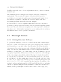
Draft MrBayes version 3.2 Manual: Tutorials and
Model Summaries
Fredrik Ronquist, John Huelsenbeck and Maxim Teslenko
November 15, 2011
2
Contents
Preface
i
1 Introduction
1
1.1
Conventions Used in this Manual . . . . . . . . . . . . . . . . . . .
2
1.2
Acquiring and Installing MrBayes . . . . . . . . . . . . . . . . . . .
2
1.3
Getting Started . . . . . . . . . . . . . . . . . . . . . . . . . . . . .
4
1.4
Changing the Size of the MrBayes Window . . . . . . . . . . . . . .
5
1.5
Getting Help . . . . . . . . . . . . . . . . . . . . . . . . . . . . . .
5
1.6
Reporting and Fixing Bugs . . . . . . . . . . . . . . . . . . . . . . .
6
1.7
License and Warranty . . . . . . . . . . . . . . . . . . . . . . . . . .
7
1.8
Citing the Program . . . . . . . . . . . . . . . . . . . . . . . . . . .
7
2 Tutorial: A Simple Analysis
9
2.1
Quick Start Version . . . . . . . . . . . . . . . . . . . . . . . . . . .
9
2.2
Thorough Version . . . . . . . . . . . . . . . . . . . . . . . . . . . . 11
2.2.1
Getting Data into MrBayes . . . . . . . . . . . . . . . . . . 11
2.2.2
Specifying a Model . . . . . . . . . . . . . . . . . . . . . . . 12
2.2.3
Setting the Priors . . . . . . . . . . . . . . . . . . . . . . . . 15
2.2.4
Checking the Model
2.2.5
Setting up the Analysis . . . . . . . . . . . . . . . . . . . . . 19
2.2.6
Running the Analysis . . . . . . . . . . . . . . . . . . . . . . 23
2.2.7
When to Stop the Analysis . . . . . . . . . . . . . . . . . . . 25
2.2.8
Summarizing Samples of Model Parameters . . . . . . . . . 27
2.2.9
Summarizing Tree Samples . . . . . . . . . . . . . . . . . . . 30
. . . . . . . . . . . . . . . . . . . . . . 18
3
4
3 Tutorial: A Partitioned Analysis
3.1 Getting Mixed Data into MrBayes
3.2 Dividing the Data into Partitions
3.3 Specifying a Partitioned Model .
3.4 Running the Analysis . . . . . . .
CONTENTS
.
.
.
.
.
.
.
.
.
.
.
.
.
.
.
.
4 More Tutorials
4.1 An Amino Acid Analysis . . . . . . . . .
4.2 Identifying Positively Selected Sites . . .
4.3 Sampling Across the GTR Model Space .
4.4 Testing a Topological Hypothesis . . . .
4.5 Testing the Strict Molecular Clock . . .
4.6 Using a Relaxed Clock Model . . . . . .
4.7 Node Dating and Total-Evidence Dating
4.8 Inferring Ancestral States . . . . . . . .
4.9 The Multi-Species Coalescent . . . . . .
5 Working with MrBayes
5.1 Reading in Data . . . . . . . . . . . .
5.2 Reading in Trees . . . . . . . . . . .
5.3 Dealing with Models . . . . . . . . .
5.3.1 Setting up a Model . . . . . .
5.3.2 Selecting a model for analysis
5.3.3 Over-parameterization . . . .
5.3.4 Bayesian Model Choice . . . .
5.3.5 Model Jumping . . . . . . . .
5.4 Starting Values . . . . . . . . . . . .
5.4.1 Default Starting Values . . . .
5.4.2 Changing Starting Values . .
5.5 Sampling the Posterior . . . . . . . .
5.5.1 Convergence and Mixing . . .
5.5.2 Proposal Mechanisms . . . . .
5.5.3 Tuning Proposals . . . . . . .
5.5.4 Monitoring Convergence . . .
.
.
.
.
.
.
.
.
.
.
.
.
.
.
.
.
.
.
.
.
.
.
.
.
.
.
.
.
.
.
.
.
.
.
.
.
.
.
.
.
.
.
.
.
.
.
.
.
.
.
.
.
.
.
.
.
.
.
.
.
.
.
.
.
.
.
.
.
.
.
.
.
.
.
.
.
.
.
.
.
.
.
.
.
.
.
.
.
.
.
.
.
.
.
.
.
.
.
.
.
.
.
.
.
.
.
.
.
.
.
.
.
.
.
.
.
.
.
.
.
.
.
.
.
.
.
.
.
.
.
.
.
.
.
.
.
.
.
.
.
.
.
.
.
.
.
.
.
.
.
.
.
.
.
.
.
.
.
.
.
.
.
.
.
.
.
.
.
.
.
.
.
.
.
.
.
.
.
.
.
.
.
.
.
.
.
.
.
.
.
.
.
.
.
.
.
.
.
.
.
.
.
.
.
.
.
.
.
.
.
.
.
.
.
.
.
.
.
.
.
.
.
.
.
.
.
.
.
.
.
.
.
.
.
.
.
.
.
.
.
.
.
.
.
.
.
.
.
.
.
.
.
.
.
.
.
.
.
.
.
.
.
.
.
.
.
.
.
.
.
.
.
.
.
.
.
.
.
.
.
.
.
.
.
.
.
.
.
.
.
.
.
.
.
.
.
.
.
.
.
.
.
.
.
.
.
.
.
.
.
.
.
.
.
.
.
.
.
.
.
.
.
.
.
.
.
.
.
.
.
.
.
.
.
.
.
.
.
.
.
.
.
.
.
.
.
.
.
.
.
.
.
.
.
.
.
.
.
.
.
.
.
.
.
.
.
.
.
.
.
.
.
.
.
.
.
.
.
.
.
.
.
.
.
.
.
.
.
.
.
.
.
.
.
.
.
.
.
.
.
.
.
.
.
.
.
.
.
.
.
.
.
.
.
.
.
.
.
.
.
.
.
.
.
.
.
.
.
.
.
.
.
.
.
.
.
.
.
.
.
.
.
37
37
38
40
42
.
.
.
.
.
.
.
.
.
45
46
48
50
52
57
62
69
78
80
.
.
.
.
.
.
.
.
.
.
.
.
.
.
.
.
85
85
87
88
88
91
95
97
98
99
99
99
99
99
99
100
101
CONTENTS
5
5.5.5 Metropolis Coupling . . . . . . . . . . . . . . . . . .
5.5.6 Improving Convergence . . . . . . . . . . . . . . . . .
5.5.7 Checkpointing . . . . . . . . . . . . . . . . . . . . . .
5.6 Stepping-stone Sampling . . . . . . . . . . . . . . . . . . . .
5.6.1 Geting started using stepping-stone sampling . . . .
5.6.2 How stepping-stone sampling works . . . . . . . . . .
5.7 Analyzing the Posterior Sample . . . . . . . . . . . . . . . .
5.7.1 Reporting Parameter Values . . . . . . . . . . . . . .
5.7.2 Convergence Diagnostics . . . . . . . . . . . . . . . .
5.7.3 Plotting . . . . . . . . . . . . . . . . . . . . . . . . .
5.7.4 Tree Summaries . . . . . . . . . . . . . . . . . . . . .
5.8 Working E↵ectively With MrBayes . . . . . . . . . . . . . .
5.8.1 Running MrBayes in Batch Mode . . . . . . . . . . .
5.8.2 Running MrBayes on a Cluster . . . . . . . . . . . .
5.8.3 Turbo-charging MrBayes with BEAGLE and MPI . .
5.9 Working with the Source Code . . . . . . . . . . . . . . . . .
5.9.1 Compiling with the GNU Tool-Chain . . . . . . . . .
5.9.2 Compiling and Running the MPI Version of MrBayes
5.9.3 Compiling the Development Version of MrBayes . . .
5.9.4 Compiling MrBayes with Xcode . . . . . . . . . . . .
5.9.5 Compiling MrBayes with Visual Studio . . . . . . . .
5.9.6 Modifying or Extending MrBayes . . . . . . . . . . .
5.10 Frequently Asked Questions . . . . . . . . . . . . . . . . . .
5.11 Di↵erences Between Versions 3.1 and 3.2 . . . . . . . . . . .
5.12 More Information . . . . . . . . . . . . . . . . . . . . . . . .
6 Evolutionary Models in MrBayes
6.1 Nucleotide Models . . . . . . . .
6.1.1 Simple Nucleotide Models
6.1.2 The Doublet Model . . . .
6.1.3 Codon Models . . . . . . .
6.2 Amino-acid Models . . . . . . . .
6.2.1 Fixed Rate Models . . . .
6.2.2 Estimating the Fixed Rate
. . . .
. . . .
. . . .
. . . .
. . . .
. . . .
Model
.
.
.
.
.
.
.
.
.
.
.
.
.
.
.
.
.
.
.
.
.
.
.
.
.
.
.
.
.
.
.
.
.
.
.
.
.
.
.
.
.
.
.
.
.
.
.
.
.
.
.
.
.
.
.
.
.
.
.
.
.
.
.
.
.
.
.
.
.
.
.
.
.
.
.
.
.
.
.
.
.
.
.
.
.
.
.
.
.
.
.
.
.
.
.
.
.
.
.
.
.
.
.
.
.
.
.
.
.
.
.
.
.
.
.
.
.
.
.
.
.
.
.
.
.
.
.
.
.
.
.
.
.
.
.
.
.
.
.
.
.
.
.
.
.
.
.
.
.
.
.
.
.
.
.
.
.
.
.
.
.
.
.
.
.
.
.
.
.
.
.
.
.
.
.
.
.
.
.
.
.
.
.
.
.
.
.
.
.
.
.
101
102
103
103
103
105
107
107
108
109
109
109
109
110
110
114
114
119
122
123
124
125
126
129
131
.
.
.
.
.
.
.
133
. 133
. 134
. 138
. 139
. 142
. 142
. 143
6
CONTENTS
6.3
6.4
6.5
6.6
6.7
6.8
6.9
6.2.3 Variable Rate Models . . . . . . . . . . . .
Restriction Site (Binary) Model . . . . . . . . . .
Standard Discrete (Morphology) Model . . . . . .
Parsimony Model . . . . . . . . . . . . . . . . . .
Rate Variation Across Sites . . . . . . . . . . . .
6.6.1 Gamma-distributed Rate Model . . . . . .
6.6.2 Autocorrelated Gamma Model . . . . . . .
6.6.3 Proportion of Invariable Sites . . . . . . .
6.6.4 Partitioned (Site Specific) Rate Model . .
6.6.5 Inferring Site Rates . . . . . . . . . . . . .
Rate Variation Across the Tree . . . . . . . . . .
6.7.1 The Covarion Model . . . . . . . . . . . .
6.7.2 Relaxed Clock Models . . . . . . . . . . .
Topology and Branch Length Models . . . . . . .
6.8.1 Unconstrained and Constrained Topology
6.8.2 Non-clock (Standard) Trees . . . . . . . .
6.8.3 Strict Clock Trees . . . . . . . . . . . . . .
6.8.4 Relaxed Clock Trees . . . . . . . . . . . .
Partitioned Models . . . . . . . . . . . . . . . . .
.
.
.
.
.
.
.
.
.
.
.
.
.
.
.
.
.
.
.
.
.
.
.
.
.
.
.
.
.
.
.
.
.
.
.
.
.
.
.
.
.
.
.
.
.
.
.
.
.
.
.
.
.
.
.
.
.
.
.
.
.
.
.
.
.
.
.
.
.
.
.
.
.
.
.
.
.
.
.
.
.
.
.
.
.
.
.
.
.
.
.
.
.
.
.
.
.
.
.
.
.
.
.
.
.
.
.
.
.
.
.
.
.
.
.
.
.
.
.
.
.
.
.
.
.
.
.
.
.
.
.
.
.
.
.
.
.
.
.
.
.
.
.
.
.
.
.
.
.
.
.
.
.
.
.
.
.
.
.
.
.
.
.
.
.
.
.
.
.
.
.
.
.
.
.
.
.
.
.
.
.
.
.
.
.
.
.
.
.
.
143
145
147
149
151
151
152
153
154
155
155
155
156
156
157
158
158
159
159
A Overview of Models and Moves
163
Bibliography
167
Preface
When we started working on MrBayes in 1999-2000, we knew that there was a
need for a Bayesian MCMC package for phylogenetics, which was more flexible
and easier to use than the software available then. Nevertheless, we were astonished by how quickly users took MrBayes to their hearts. The original release paper (Huelsenbeck and Ronquist, 2001), which appeared in Bioinformatics in 2001,
quickly became a fast-track paper in Computer Science, as did the release note for
version 3 (Ronquist and Huelsenbeck, 2003), published in Bioinformatics in 2003.
To date, these two papers have accumulated more than 13,000 citations.
With the release of version 3.2 (Ronquist et al., 2011), MrBayes has come of
age. Through the years, we have added to, extended, and rewritten the program
to cover most of the models used in standard statistical phylogenetic analyses
today. We have also implemented a number of techniques to speed up calculations,
improve convergence, and facilitate Bayesian model averaging and model choice.
Version 3.2 has also undergone considerably more testing than previous versions
of MrBayes. This is not to say that MrBayes 3.2 is bug free but it should be
considerably more stable than previous versions. As in previous versions, we have
done our best to document all of the available models and tools in the online help
and in this manual.
Version 3.2 of MrBayes also marks the end of the road for us in terms of major
development. Extending the original code has become increasingly difficult, and
with version 3.2 we are at a point where we feel we need to explore new approaches
to Bayesian phylogenetics. Perhaps most importantly, model specifications in MrBayes are strongly limited by the constraints of the Nexus language. In a separate
project, RevBayes, we hope to provide a generic computing environment that ali
ii
PREFACE
lows users to build complex phylogenetic models interactively, from small building
blocks. However, such flexibility requires more of the user, and it may not be
popular with everyone. For standard analyses, MrBayes will remain adequate for
years to come and it is our intention to maintain the code base as long as the
program remains heavily used and we have the resources to do so.
The MrBayes project would not have been possible without the help from many
people. First and foremost, we would like to thank Maxim Teslenko, who has
played an important role in fixing bugs and adding functionality to MrBayes during
the last couple of years. Among other things, Maxim is responsible for a large part
of the work involved in supporting BEAGLE, and in implementing the steppingstone method for estimating marginal likelihoods. Maxim has also contributed
several sections to this manual.
We are grateful for the financial support of the project provided by the Swedish
Research Council, the National Institutes of Health, and the National Science
Foundation. We are also deeply indebted to students, colleagues and numerous
users of MrBayes, who have helped the project along in important ways. We are
not going to try to enumerate them here, as any attempt to do so is likely to result
in major omissions. However, we do want to express the overwhelming feeling of
gratitude we feel for the generosity with which people have shared ideas, bug fixes
and other valuable tips through the years. This feedback alone makes all the hours
we have put into developing MrBayes worthwhile. Thank you, all of you!
Last but not least, we would like to thank our families for the unwavering support
they have provided throughout the project. During intense programming periods,
or when we have taught MrBayes workshops around the world, they have had to
cope with absent-minded fathers, aloof visitors, and absent husbands. We realize
that the childish enthusiasm we have shown when a new model resulted in some
incomprehensible numbers scrolling by on the screen has been poor compensation.
Thank you so much for all of your support and your sacrifices; we love you!
November, 2011
Fredrik Ronquist
John Huelsenbeck
Chapter 1
Introduction
MrBayes 3 is a program for Bayesian inference and model choice across a large
space of phylogenetic and evolutionary models. The program has a
command-line interface and should run on a variety of computer platforms,
including large computer clusters and multicore machines. Depending on the
settings, MrBayes analyses may demand a lot of your machine, both in terms of
memory and processor speed. Many users therefore run more challenging
analyses on dedicated computing machines or clusters. Several computing centers
around the globe provide web access to such services. This said, many standard
analyses run fine on common desktop machines.
This manual explains how to use the program. After introducing you to the
program in this chapter, we first walk you through a simple analysis (chapter 2),
which will get you started, and a more complex partitioned analysis, which uses
more of the program’s capabilities (chapter 3). This is followed by a set of
shorter tutorials covering a range of common types of analyses (chapter 4).
We then cover the capabilities of the program in more detail (chapter 5), followed
by some details on the evolutionary models that are implemented (chapter 6).
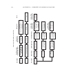
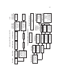
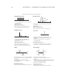
The manual ends with a series of diagrams giving a graphical overview of the
models and some proposal mechanisms implemented in the program (Appendix
A). For more detailed information about commands and options in MrBayes, see
the command reference that can either be downloaded from the program web site
1
2
CHAPTER 1. INTRODUCTION
or generated from the program itself (see section 1.5 below). All the information
in the command reference is also available on-line when using the program.
The manual assumes that you are familiar with the basic concepts of Bayesian
phylogenetics. If you are new to the subject, we recommend one of several recent
reviews (Lewis, 2001; Holder and Lewis, 2003; Ronquist and Deans, 2010). The
early papers introducing Bayesian phylogenetic methods (Li, 1996; Mau, 1996;
Rannala and Yang, 1996; Mau and Newton, 1997; Larget and Simon, 1999; Mau
et al., 1999; Newton et al., 1999) are also worthwhile reading. The basic MCMC
techniques are described in Metropolis et al. (1953) and Hastings (1970), and the
Metropolis-coupled MCMC used by MrBayes was introduced by Geyer (1991).
Some recent general textbooks on Bayesian inference and MCMC methods
include Gilks et al. (1996), Carlin and Louis (2000), Gelman et al. (2003), and
Gamerman and Lopes (2006).
1.1
Conventions Used in this Manual
Throughout the document, we use typewriter font for things you see on screen
or in a data file, and bold font for things you should type in. Alternative
commands, options, file names, etc are also given in typewriter font.
1.2
Acquiring and Installing MrBayes
MrBayes 3 is distributed without charge by download from the MrBayes web
site, http://mrbayes.net. If someone has given you a copy of MrBayes 3, we
strongly suggest that you download the most recent version from the official
MrBayes site. The site also gives information about the MrBayes users email list
and describes how you can report bugs or contribute to the project.
MrBayes 3 is a plain-vanilla program that uses a command line interface and
therefore behaves virtually the same on all platforms — Macintosh, Windows
and Unix. There is a separate download for each platform. The Windows and
Macintosh downloads contain an installer that will install the program for you.
1.2. ACQUIRING AND INSTALLING MRBAYES
3
The Macintosh installer will put an executable in a default location that should
be in your path. After installation, you run MrBayes by opening a terminal
window (for instance using the Terminal application, which you will find in the
Utilities folder in your Applications folder), and then simply typing mb on the
command line. The example data files and the documentation are installed in a
MrBayes folder in your Applications directory.
The Macintosh installer will also install the BEAGLE library, which you can use
to speed up likelihood calculations. The BEAGLE option is particularly useful if
you have an NVIDIA graphics card and the relevant CUDA drivers installed, in
which case MCMC sampling from amino acid and codon models should be much
faster. The installer will provide you with a link that you can use to download
and install the relevant drivers given that you have an NVIDIA graphics card. If
the CUDA drivers are not installed (or if you do not have an NVIDIA graphics
card), then BEAGLE will run on the CPU instead of on the GPU. In this case,
the BEAGLE performance will be similar to that of the default likelihood
calculators used by MrBayes.
The Windows installer behaves similarly to the Macintosh installer except that it
places a double-clickable executable in the MrBayes folder inside your Program
directory, together with the example files and the documentation. To start the
program, simply double-click on the executable. The Windows installer will also
install the BEAGLE library, and it will give you a link to the relevant CUDA
drivers.
If you decide to run the program under Unix/Linux, then you need to compile
the program from source code. You can find detailed compilation instructions in
chapter 5. Once you have compiled MrBayes, you will get an executable called
mb. To execute the program, simply type ./mb in the directory where you
compiled the program. If you execute make install after compilation, the
binary is installed in your path and you can then invoke MrBayes by typing mb
from any directory on your system.
The Macintosh and Windows installers will install the serial version of the
program. The serial version does not support multithreading, which means that
you will not be able to utilize more than one core on a multi-core machine for a
4
CHAPTER 1. INTRODUCTION
single MrBayes analysis. If you want to utilize all cores, you need to run the
MPI-version of MrBayes. The MPI-version must be compiled from source and
will only run under Unix/Linux. Most Windows machines allow you to install a
parallel Linux partition, and all modern Macintosh computers come with a Unix
system under the hood, which will support MPI. Refer to chapter 5 for more
detailed instructions on how to compile and run the MPI version of MrBayes.
All three packages of MrBayes come with example data files. These are intended
to show various types of analyses you can perform with the program, and you
can use them as templates for your own analyses. In the tutorials given in
chapters 2 to 4, you can learn more about how to set up various types of analyses
based on these example data files.
1.3
Getting Started
Start MrBayes by double-clicking the application icon (or typing ./mb or simply
mb depending on your system) and you will see the information below:
MrBayes v3.2
(Bayesian Analysis of Phylogeny)
Distributed under the GNU General Public License
Type "help" or "help <command>" for information
on the commands that are available.
Type "about" for authorship and general
information about the program.
MrBayes >
Note the MrBayes > prompt at the bottom, which tells you that MrBayes is
ready for your commands.
1.4. CHANGING THE SIZE OF THE MRBAYES WINDOW
1.4
5
Changing the Size of the MrBayes Window
Some MrBayes commands will output a lot of information and write fairly long
lines, so you may want to change the size of the MrBayes window to make it
easier to read the output. On Macintosh and Unix machines, you should be able
to increase the window size simply by dragging the margins. On a Windows
machine, you cannot increase the size of the window beyond the preset value by
simply dragging the margins but you can change both the size of the screen
bu↵er and the console window by right-clicking on the blue title bar of the
MrBayes window and then selecting “Properties” in the menu that appears.
Make sure the “Layout” tab is selected in the window that appears, and then set
the Screen Bu↵er Size and Window Size to the desired values.
1.5
Getting Help
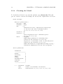
At the MrBayes > prompt, type help to see a list of the commands available in
MrBayes. Most commands allow you to set values (options) for di↵erent
parameters. If you type help <command> , where <command> is any of the listed
commands, you will see the help information for that command as well as a
description of the available options. For most commands, you will also see a list
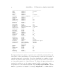
of the current settings at the end. Try, for instance, help lset or help mcmc .
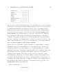
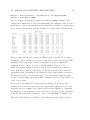
The lset settings table at the end should look like this:
Parameter
Options
Current Setting
-----------------------------------------------------------------Nucmodel
4by4/Doublet/Codon/Protein
4by4
Nst
1/2/6/Mixed
1
Code
Universal/Vertmt/Mycoplasma/
Yeast/Ciliates/Metmt
Universal
Ploidy
Haploid/Diploid/Zlinked
Diploid
Rates
Equal/Gamma/Propinv/Invgamma/Adgamma Equal
Ngammacat
<number>
4
Nbetacat
<number>
5
Omegavar
Equal/Ny98/M3
Equal
Covarion
No/Yes
No
Coding
All/Variable/Noabsencesites/
6
CHAPTER 1. INTRODUCTION
Nopresencesites
All
Parsmodel
No/Yes
No
------------------------------------------------------------------
Note that MrBayes 3 supports abbreviations of commands and options, so in
many cases it is sufficient to type the first few letters of a command or option
instead of the full name.
A complete list of commands and options is given in the command reference,
which can be downloaded from the program web site (www.mrbayes.net). You
can also produce an ASCII text version of the command reference at any time by
giving the command manual to MrBayes. Finally, you can get in touch with
other MrBayes users and developers through the mrbayes-users email list
(subscription information at www.mrbayes.net).
1.6
Reporting and Fixing Bugs
If you find a bug in MrBayes, we are grateful if you tell us about it using the bug
reporting functions of SourceForge, as explained on the MrBayes web site
(www.mrbayes.net). When you submit a bug report, make sure that you upload
a data file with the data set and sequence of commands that produced the error.
If the bug occurs during an MCMC analysis (after issuing the mcmc command),
you can help us greatly by making sure the bug can be reproduced reliably using
a fixed seed and swapseed . These seeds need to be set by invoking the set
command before any other commands are executed, including the reading in of
data. When data are read in, a default model is automatically set up, with initial
values drawn randomly using the current seeds, so resetting the seeds after the
data are read in is not guaranteed to result in the same MCMC output. Ideally,
it should also be possible to reproduce the bug with a small data set and using as
few MCMC generations as possible. The most common mistake is to report a
bug without including a dataset or an e-mail address, pretty much making it
impossible for us to fix the problem.
Advanced users may be interested in fixing bugs themselves in the source code.
Refer to section 5 of this manual for information on how to contribute bug fixes,
1.7. LICENSE AND WARRANTY
7
improved algorithms or expanded functionality to other users of MrBayes.
1.7
License and Warranty
MrBayes is free software; you can redistribute it and/or modify it under the
terms of the GNU General Public License as published by the Free Software
Foundation; either version 3 of the License, or (at your option) any later version.
The program is distributed in the hope that it will be useful, but WITHOUT
ANY WARRANTY; without even the implied warranty of
MERCHANTABILITY or FITNESS FOR A PARTICULAR PURPOSE. See the
GNU General Public License for more details
(http://www.gnu.org/copyleft/gpl.html).
1.8
Citing the Program
If you wish to cite the program, you can simply refer to the most recent release
note (Ronquist et al., 2011). This manual should be cited as an online
publication. For more tips on citations, you can run the citations command in
the program, which will give you a number of other relevant citations for the
program and its models and algorithms.
8
CHAPTER 1. INTRODUCTION
Chapter 2
Tutorial: A Simple Analysis
This section walks you through a simple MrBayes example analysis to get you
started. It is based on the primates.nex data file and will guide you through a
basic Bayesian MCMC analysis of phylogeny, explaining the most important
features of the program. There are two versions of the tutorial. You will first find
a Quick-Start version for impatient users who want to get an analysis started
immediately. The rest of the section contains a much more detailed description
of the same analysis.
2.1
Quick Start Version
There are four steps to a typical Bayesian phylogenetic analysis using MrBayes:
1. Read the Nexus data file
2. Set the evolutionary model
3. Run the analysis
4. Summarize the samples
In more detail, each of these steps is performed as described in the following
paragraphs:
9
10
CHAPTER 2. TUTORIAL: A SIMPLE ANALYSIS
1. At the MrBayes > prompt, type execute primates.nex. This will bring the
data into the program. When you only give the data file name (primates.nex),
MrBayes assumes that the file is in the current directory. If this is not the case,
you have to use the full or relative path to your data file, for example execute
../taxa/primates.nex. If you are running your own data file for this tutorial,
beware that it may contain some MrBayes commands that can change the
behavior of the program; delete those commands or put them in square brackets
to follow this tutorial.
2. At the MrBayes > prompt, type lset nst=6 rates=invgamma. This sets
the evolutionary model to the GTR substitution model with gamma-distributed
rate variation across sites and a proportion of invariable sites. If your data are
not DNA or RNA, if you want to invoke a di↵erent model, or if you want to use
non-default priors, refer to the rest of this manual and the Appendix for more
help.
3.1. At the MrBayes > prompt, type mcmc ngen=20000 samplefreq=100
printfreq=100 diagnfreq=1000. This will ensure that you get at least 200
samples from the posterior probability distribution, and that diagnostics are
calculated every 1,000 generations. For larger data sets you probably want to run
the analysis longer and sample less frequently. The default sample and print
frequency is 500, the default diagnostic frequency is 5,000, and the default run
length is 1,000,000. You can find the predicted remaining time to completion of
the analysis in the last column printed to screen.
3.2. If the standard deviation of split frequencies is below 0.01 after 20,000
generations, stop the run by answering no when the program asks Continue the
analysis? (yes/no). Otherwise, keep adding generations until the value falls
below 0.01. If you are interested mainly in the well-supported parts of the tree, a
standard deviation below 0.05 may be adequate.
4.1. Type sump to summarize the parameter values using the same burn-in as
the diagnostics in the mcmc command. The program will output a table with
summaries of the samples of the substitution model parameters, including the
mean, mode, and 95 % credibility interval (region of Highest Posterior Density,
HPD) of each parameter. Make sure that the potential scale reduction factor
2.2. THOROUGH VERSION
11
(PSRF) is reasonably close to 1.0 for all parameters; if not, you need to run the
analysis longer.
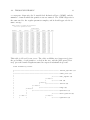
4.2. Summarize the trees using the same burn-in as the mcmc command by
typing sumt . The program will output a cladogram with the posterior
probabilities for each split and a phylogram with mean branch lengths. Both
trees will also be printed to a file that can be read by FigTree and other
tree-drawing programs, such as TreeView and Mesquite.
It does not have to be more complicated than this; however, as you get more
proficient you will probably want to know more about what is happening behind
the scenes. The rest of this section explains each of the steps in more detail and
introduces you to all the implicit assumptions you are making and the machinery
that MrBayes uses in order to perform your analysis.
2.2
2.2.1
Thorough Version
Getting Data into MrBayes
To get data into MrBayes, you need a so-called Nexus file that contains aligned
nucleotide or amino acid sequences, morphological (”standard”) data, restriction
site (binary) data, or any mix of these four data types. The Nexus data file is
often generated by another program, such as Mesquite (Maddison and Maddison,
2006). Note, however, that MrBayes version 3 does not support the full Nexus
standard, so you may have to do a little editing of the file for MrBayes to process
it properly. In particular, MrBayes uses a fixed set of symbols for each data type
and does not support user-defined symbols. The supported symbols are {A, C,
G, T, R, Y, M, K, S, W, H, B, V, D, N} for DNA data, {A, C, G, U, R, Y, M,
K, S, W, H, B, V, D, N} for RNA data, {A, R, N, D, C, Q, E, G, H, I, L, K, M,
F, P, S, T, W, Y, V, X} for protein data, {0, 1} for restriction (binary) data, and
{0, 1, 2, 3, 4, 5, 6, 5, 7, 8, 9} for standard (morphology) data. In addition to the
standard one-letter ambiguity symbols for DNA and RNA listed above, ambiguity
can also be expressed using the Nexus parenthesis or curly braces notation. For
instance, a taxon polymorphic for states 2 and 3 can be coded as (23), (2,3),
12
CHAPTER 2. TUTORIAL: A SIMPLE ANALYSIS
{23}, or {2,3} and a taxon with either amino acid A or F can be coded as (AF),
(A,F), {AF} or {A,F}. Like most other statistical phylogenetics programs,
MrBayes e↵ectively treats polymorphism and uncertainty the same way (as
uncertainty), so it does not matter whether you use parentheses or curly braces.
If you have other symbols in your matrix than the ones supported by MrBayes,
you need to replace them before processing the data block in MrBayes. You also
need to remove the ”Equate” and ”Symbols” statements in the ”Format” line if
they are included. Unlike the Nexus standard, MrBayes supports data blocks
that contain mixed data types as described in the tutorial in chapter 3.
To put the data into MrBayes type execute <filename> at the MrBayes >
prompt, where <filename> is the name of the input file. To process our
example file, type execute primates.nex or simply exe primates.nex to save
some typing (MrBayes allows you to use the shortest unambiguous version of a
command). Note that the input file must be located in the same folder
(directory) where you started the MrBayes application (or else you will have to
give the path to the file) and the name of the input file should not have blank
spaces, or it will have to be quoted. If everything proceeds normally, MrBayes
will acknowledge that it has read the data in the DATA block of the Nexus file
by outputting some information about the file read in.
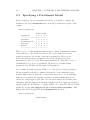
2.2.2
Specifying a Model
All of the commands are entered at the MrBayes > prompt. At a minimum two
commands, lset and prset, are required to specify the evolutionary model that
will be used in the analysis. Usually, it is also a good idea to check the model
settings prior to the analysis using the showmodel command. In general, lset is
used to define the structure of the model and prset is used to define the prior
probability distributions on the parameters of the model. In the following, we
will specify a GTR + I + model (a General Time Reversible model with a
proportion of invariable sites and a gamma-shaped distribution of rates across
sites) for the evolution of the mitochondrial sequences and we will check all of
the relevant priors. We assume that you are familiar with the common stochastic
models of molecular evolution.
2.2. THOROUGH VERSION
13
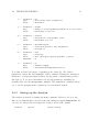
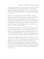
In general, a good start is to type help lset. Ignore the help information for now
and concentrate on the table at the bottom of the output, which specifies the
current settings. It should look like this:
Model settings for partition 1:
Parameter
Options
Current Setting
-----------------------------------------------------------------Nucmodel
4by4/Doublet/Codon/Protein
4by4
Nst
1/2/6/Mixed
1
Code
Universal/Vertmt/Mycoplasma/
Yeast/Ciliates/Metmt
Universal
Ploidy
Haploid/Diploid/Zlinked
Diploid
Rates
Equal/Gamma/Propinv/Invgamma/Adgamma Equal
Ngammacat
<number>
4
Nbetacat
<number>
5
Omegavar
Equal/Ny98/M3
Equal
Covarion
No/Yes
No
Coding
All/Variable/Noabsencesites/
Nopresencesites
All
Parsmodel
No/Yes
No
------------------------------------------------------------------
First, note that the table is headed by Model settings for partition 1. By
default, MrBayes divides the data into one partition for each type of data you
have in your DATA block. If you have only one type of data, all data will be in a
single partition by default. How to change the partitioning of the data will be
explained in the tutorial in chapter 3.
The Nucmodel setting allows you to specify the general type of DNA model. The
Doublet option is for the analysis of paired stem regions of ribosomal DNA and
the Codon option is for analyzing the DNA sequence in terms of its codons. We
will analyze the data using a standard nucleotide substitution model, in which
case the default 4by4 option is appropriate, so we will leave Nucmodel at its
default setting.
The general structure of the substitution model is determined by the Nst setting.
By default, all substitutions have the same rate (Nst=1), corresponding to the
F81 model (or the JC model if the stationary state frequencies are forced to be
equal using the prset command, see below). We want the GTR model (Nst=6)
14
CHAPTER 2. TUTORIAL: A SIMPLE ANALYSIS
instead of the F81 model so we type lset nst=6. MrBayes should acknowledge
that it has changed the model settings.
The Code setting is only relevant if the Nucmodel is set to Codon. The Ploidy
setting is also irrelevant for us. However, we need to change the Rates setting
from the default Equal (no rate variation across sites) to Invgamma
(gamma-shaped rate variation with a proportion of invariable sites). Do this by
typing lset rates=invgamma. Again, MrBayes will acknowledge that it has
changed the settings. We could have changed both lset settings at once if we
had typed lset nst=6 rates=invgamma in a single line.
We will leave the Ngammacat setting (the number of discrete categories used to
approximate the gamma distribution) at the default of 4. In most cases, four rate
categories are sufficient. It is possible to increase the accuracy of the likelihood
calculations by increasing the number of rate categories. However, the time it
will take to complete the analysis will increase in direct proportion to the
number of rate categories you use, and the e↵ects on the results will be negligible
in most cases.
Of the remaining settings, it is only Covarion and Parsmodel that are relevant
for single nucleotide models. We will use neither the parsimony model nor the
covariotide model for our data, so we will leave these settings at their default
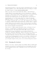
values. If you type help lset now to verify that the model is correctly set, the
table should look like this:
Model settings for partition 1:
Parameter
Options
Current Setting
-----------------------------------------------------------------Nucmodel
4by4/Doublet/Codon/Protein
4by4
Nst
1/2/6/Mixed
6
Code
Universal/Vertmt/Mycoplasma/
Yeast/Ciliates/Metmt
Universal
Ploidy
Haploid/Diploid/Zlinked
Diploid
Rates
Equal/Gamma/Propinv/Invgamma/Adgamma Invgamma
Ngammacat
<number>
4
Nbetacat
<number>
5
Omegavar
Equal/Ny98/M3
Equal
Covarion
No/Yes
No
2.2. THOROUGH VERSION
15
Coding
All/Variable/Noabsencesites/
Nopresencesites
All
Parsmodel
No/Yes
No
------------------------------------------------------------------
2.2.3
Setting the Priors
We now need to set the priors for our model. There are six types of parameters
in the model: the topology, the branch lengths, the four stationary frequencies of
the nucleotides, the six di↵erent nucleotide substitution rates, the proportion of
invariable sites, and the shape parameter of the gamma distribution of rate
variation. The default priors in MrBayes work well for most analyses, and we will
not change any of them for now. By typing help prset you can obtain a list of
the default settings for the parameters in your model. The table at the end of
the help information reads:
Model settings for partition 1:
Parameter
Options
Current Setting
-----------------------------------------------------------------Tratiopr
Beta/Fixed
Beta(1.0,1.0)
Revmatpr
Dirichlet/Fixed
Dirichlet(1.0,1.0,...
Aamodelpr
Fixed/Mixed
Fixed(Poisson)
Aarevmatpr
Dirichlet/Fixed
Dirichlet(1.0,1.0,...)
Omegapr
Dirichlet/Fixed
Dirichlet(1.0,1.0)
Ny98omega1pr
Beta/Fixed
Beta(1.0,1.0)
Ny98omega3pr
Uniform/Exponential/Fixed
Exponential(1.0)
M3omegapr
Exponential/Fixed
Exponential
Codoncatfreqs
Dirichlet/Fixed
Dirichlet(1.0,1.0,1.0)
Statefreqpr
Dirichlet/Fixed
Dirichlet(1.0,1.0,...
Shapepr
Uniform/Exponential/Fixed
Uniform(0.0,200.0)
Ratecorrpr
Uniform/Fixed
Uniform(-1.0,1.0)
Pinvarpr
Uniform/Fixed
Uniform(0.0,1.0)
Covswitchpr
Uniform/Exponential/Fixed
Uniform(0.0,100.0)
Symdirihyperpr
Uniform/Exponential/Fixed
Fixed(Infinity)
Topologypr
Uniform/Constraints/Fixed
Uniform
Brlenspr
Unconstrained/Clock/Fixed
Unconstrained:Exp(10.0)
Treeagepr
Exponential/Gamma/Fixed
Exponential(1.0)
Speciationpr
Uniform/Exponential/Fixed
Exponential(1.0)
16
CHAPTER 2. TUTORIAL: A SIMPLE ANALYSIS
Extinctionpr
SampleStrat
Sampleprob
Popsizepr
Beta/Fixed
Beta(1.0,1.0)
Random/Diversity/Cluster
Random
<number>
1.00
Lognormal/Gamma/Uniform/
Lognormal(4.6,2.3)
Normal/Fixed
Popvarpr
Equal/Variable
Equal
Nodeagepr
Unconstrained/Calibrated
Unconstrained
Clockratepr
Fixed/Normal/Lognormal/
Exponential/Gamma
Fixed
Clockvarpr
Strict/Cpp/TK02/Igr
Strict
Cppratepr
Fixed/Exponential
Exponential(0.10)
Cppmultdevpr
Fixed
Fixed(0.40)
TK02varpr
Fixed/Exponential/Uniform
Exponential(10.00)
Ratepr
Fixed/Variable=Dirichlet
Fixed
------------------------------------------------------------------
We need to focus on Revmatpr (for the six substitution rates of the GTR rate
matrix), Statefreqpr (for the stationary nucleotide frequencies of the GTR rate
matrix), Shapepr (for the shape parameter of the gamma distribution of rate
variation), Pinvarpr (for the proportion of invariable sites), Topologypr (for the
topology), and Brlenspr (for the branch lengths).
The default prior probability density is a flat Dirichlet (all values are 1.0) for
both Revmatpr and Statefreqpr. This is appropriate if we want estimate these
parameters from the data assuming no prior knowledge about their values. It is
possible to fix the rates and nucleotide frequencies but this is generally not
recommended. However, it is occasionally necessary to fix the nucleotide
frequencies to be equal, for instance in specifying the JC and SYM models. This
would be achieved by typing prset statefreqpr=fixed(equal).
If we wanted to specify a prior that put more emphasis on equal nucleotide
frequencies than the default flat Dirichlet prior, we could for instance use prset
statefreqpr = Dirichlet(10,10,10,10) or, for even more emphasis on equal
frequencies, prset statefreqpr=Dirichlet(100,100,100,100). The sum of
the numbers in the Dirichlet distribution determines how focused the distribution
is, and the balance between the numbers determines the expected proportion of
each nucleotide (in the order A, C, G, and T). Usually, there is a connection
between the parameters in the Dirichlet distribution and the observations. For
example, you can think of a Dirichlet (150,100,90,140) distribution as one arising
2.2. THOROUGH VERSION
17
from observing (roughly) 150 A’s, 100 C’s, 90 G’s and 140 T’s in some set of
reference sequences. If the reference sequences are independent but clearly
relevant to the analysis of your sequences, it might be reasonable to use those
numbers as a prior in your analysis.
In our analysis, we will be cautious and leave the prior on state frequencies at its
default setting. If you have changed the setting according to the suggestions
above, you need to change it back by typing prset statefreqpr =
Dirichlet(1,1,1,1) or prs st = Dir(1,1,1,1) if you want to save some typing.
Similarly, we will leave the prior on the substitution rates at the default flat
Dirichlet(1,1,1,1,1,1) distribution.
The Shapepr parameter determines the prior for the ↵ (shape) parameter of the
gamma distribution of rate variation. We will leave it at its default setting, a
uniform distribution spanning a wide range of ↵ values. The prior for the
proportion of invariable sites is set with Pinvarpr. The default setting is a
uniform distribution between 0 and 1, an appropriate setting if we don’t want to
assume any prior knowledge about the proportion of invariable sites.
For topology, the default Uniform setting for the Topologypr parameter puts
equal probability on all distinct, fully resolved topologies. The alternative is to
introduce some constraints on the tree topology, but we will not attempt that in
this analysis.
The Brlenspr parameter can either be set to unconstrained or clock-constrained.
For trees without a molecular clock (unconstrained) the branch length prior can
be set either to exponential or uniform. The default exponential prior with
parameter 10.0 should work well for most analyses. It has an expectation of
1/10 = 0.1 but allows a wide range of branch length values (theoretically from 0
to infinity). Because the likelihood values vary much more rapidly for short
branches than for long branches, an exponential prior on branch lengths usually
works better than a uniform prior.
18
CHAPTER 2. TUTORIAL: A SIMPLE ANALYSIS
2.2.4
Checking the Model
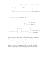
To check the model before we start the analysis, type showmodel. This will
give an overview of the model settings. In our case, the output will be as follows:
Model settings:
Data not partitioned -Datatype = DNA
Nucmodel = 4by4
Nst
= 6
Substitution rates, expressed as proportions
of the rate sum, have a Dirichlet prior
(1.00,1.00,1.00,1.00,1.00,1.00)
Covarion = No
# States = 4
State frequencies have a Dirichlet prior
(1.00,1.00,1.00,1.00)
Rates
= Invgamma
Gamma shape parameter is uniformly distributed on the interval (0.00,200.00).
Proportion of invariable sites is uniformly distributed on the interval (0.00,1.00).
Gamma distribution is approximated using 4 categ...
Likelihood summarized over all rate categories ...
Active parameters:
Parameters
-----------------Revmat
1
Statefreq
2
Shape
3
Pinvar
4
Ratemultiplier
5
Topology
6
Brlens
7
-----------------1 --
Parameter
Type
Prior
= Revmat
= Rates of reversible rate matrix
= Dirichlet(1.00,1.00,1.00,1.00,1.00,1.00)
2.2. THOROUGH VERSION
19
2 --
Parameter
Type
Prior
= Pi
= Stationary state frequencies
= Dirichlet
3 --
Parameter
Type
Prior
= Alpha
= Shape of scaled gamma distribution of site rates
= Uniform(0.00,200.00)
4 --
Parameter
Type
Prior
= Pinvar
= Proportion of invariable sites
= Uniform(0.00,1.00)
5 --
Parameter
Type
Prior
= Ratemultiplier
= Partition-specific rate multiplier
= Fixed(1.0)
6 --
Parameter
Type
Prior
Subparam.
=
=
=
=
7 --
Parameter
Type
Prior
= V
= Branch lengths
= Unconstrained:Exponential(10.0)
Tau
Topology
All topologies equally probable a priori
V
Note that we have seven types of parameters in our model. All of these
parameters, except the rate multiplier, will be estimated during the analysis (to
fix them to some predetermined values, use the prset command and specify a
fixed prior). To see more information about each parameter, including its
starting value, use the showparams command. The startvals command allows
one to set the starting values, separately for each chain if desired.
2.2.5
Setting up the Analysis
The analysis is started by issuing the mcmc command. However, before doing
this, we recommend that you review the run settings by typing help mcmc. In
our case, we will get the following table at the bottom of the output:
Parameter
Options
Current Setting
20
CHAPTER 2. TUTORIAL: A SIMPLE ANALYSIS
----------------------------------------------------Ngen
<number>
1000000
Nruns
<number>
2
Nchains
<number>
4
Temp
<number>
0.100000
Reweight
<number>,<number>
0.00 v 0.00 ^
Swapfreq
<number>
1
Nswaps
<number>
1
Samplefreq
<number>
500
Printfreq
<number>
500
Printall
Yes/No
Yes
Printmax
<number>
8
Mcmcdiagn
Yes/No
Yes
Diagnfreq
<number>
5000
Diagnstat
Avgstddev/Maxstddev
Avgstddev
Minpartfreq
<number>
0.10
Allchains
Yes/No
No
Allcomps
Yes/No
No
Relburnin
Yes/No
Yes
Burnin
<number>
0
Burninfrac
<number>
0.25
Stoprule
Yes/No
No
Stopval
<number>
0.05
Savetrees
Yes/No
No
Checkpoint
Yes/No
Yes
Checkfreq
<number>
100000
Filename
<name>
primates.nex.<p/t>
Startparams
Current/Reset
Current
Starttree
Current/Random/
Current
Parsimony
Nperts
<number>
0
Data
Yes/No
Yes
Ordertaxa
Yes/No
No
Append
Yes/No
No
Autotune
Yes/No
Yes
Tunefreq
<number>
100
---------------------------------------------------------------------------
The Ngen setting is the number of generations for which the analysis will be run.
It is useful to run a small number of generations first to make sure the analysis is
correctly set up and to get an idea of how long it will take to complete a longer
analysis. We will start with 20,000 generations but you may want to start with
an even smaller number for a larger data set. To change the Ngen setting without
starting the analysis we use the mcmcp command, which is equivalent to mcmc
except that it does not start the analysis. Type mcmcp ngen=20000 to set the
number of generations to 20,000. You can type help mcmc to confirm that the
2.2. THOROUGH VERSION
21
setting was changed appropriately.
By default, MrBayes will run two simultaneous, completely independent analyses
starting from di↵erent random trees (Nruns = 2). Running more than one
analysis simultaneously allows MrBayes to calculate convergence diagnostics on
the fly, which is helpful in determining when you have a good sample from the
posterior probability distribution. The idea is to start each run from a di↵erent,
randomly chosen tree. In the early phases of the run, the two runs will sample
very di↵erent trees but when they have reached convergence (when they produce
a good sample from the posterior probability distribution), the two tree samples
should be very similar.
To make sure that MrBayes compares tree samples from the di↵erent runs, check
that Mcmcdiagn is set to yes and that Diagnfreq is set to some reasonable value.
The default value of 5000 is more appropriate for a larger analysis, so change the
setting so that we compute diagnostics every 1000th generation instead by typing
mcmcp diagnfreq=1000.
MrBayes will now calculate various run diagnostics every Diagnfreq generation
and print them to a file with the name <Filename>.mcmc. The most important
diagnostic, a measure of the similarity of the tree samples in the di↵erent runs,
will also be printed to screen every Diagnfreq generation. Every time the
diagnostics are calculated, either a fixed number of samples (burnin) or a
percentage of samples (burninfrac) from the beginning of the chain is discarded.
The relburnin setting determines whether a fixed burnin (relburnin=no) or a
burnin percentage (relburnin=yes) is used. By default, MrBayes will discard the
first 25 % samples from the cold chain (relburnin=yes and burninfrac=0.25).
By default, MrBayes uses Metropolis coupling to improve the MCMC sampling
of the target distribution. The Swapfreq, Nswaps, Nchains, and Temp settings
together control the Metropolis coupling behavior. When Nchains is set to 1, no
heating is used. When Nchains is set to a value n larger than 1, then n 1
heated chains are used. By default, Nchains is set to 4, meaning that MrBayes
will use 3 heated chains and one “cold” chain. In our experience, heating is
essential for some data sets but it is not needed for others. Adding more than
three heated chains may be helpful in analyzing large and difficult data sets. The
22
CHAPTER 2. TUTORIAL: A SIMPLE ANALYSIS
time complexity of the analysis is directly proportional to the number of chains
used (unless MrBayes runs out of physical RAM memory, in which case the
analysis will suddenly become much slower), but the cold and heated chains can
be distributed among processors in a cluster of computers and among cores in
multicore processors using the MPI version of the program, greatly speeding up
the calculations.
MrBayes uses an incremental heating scheme, in which chain i is heated by
raising its posterior probability to the power 1/(1 + i ), where is the heating
coefficient controlled by the Temp parameter. Every Swapfreq generation, two
chains are picked at random and an attempt is made to swap their states. For
many analyses, the default settings should work nicely. If you are running many
more than three heated chains, however, you may want to increase the number of
swaps (Nswaps) that are tried each time the chain stops for swapping. If the
frequency of swapping between chains that are adjacent in temperature is low,
you may want to decrease the Temp parameter.
The Samplefreq setting determines how often the chain is sampled; the default
is every 500 generations. This works well for moderate-sized analyses but our
analysis is so small and is likely to converge so rapidly that it makes sense to
sample more often. Let us sample the chain every 100th generation instead by
typing mcmcp samplefreq=100. For really large data sets that take a long
time to converge, you may even want to sample less frequently than the default,
or you will end up with very large files containing tree and parameter samples.
When the chain is sampled, the current values of the model parameters are
printed to file. The substitution model parameters are printed to a .p file (in our
case, there will be one file for each independent analysis, and they will be called
primates.nex.run1.p and primates.nex.run2.p). The .p files are tab
delimited text files that can be imported into most statistics and graphing
programs. The topology and branch lengths are printed to a .t file (in our case,
there will be two files called primates.nex.run1.t and primates.nex.run2.t).
The .t files are Nexus tree files that can be imported into programs like PAUP*
and TreeView. The root of the .p and .t file names can be altered using the
Filename setting.
2.2. THOROUGH VERSION
23
The Printfreq parameter controls the frequency with which brief info about the
analysis is printed to screen. The default value is 500. Let us change it to match
the sample frequency by typing mcmcp printfreq=100.
When you set up your model and analysis (the number of runs and heated
chains), MrBayes creates starting values for the model parameters. A di↵erent
random tree with predefined branch lengths is generated for each chain and most
substitution model parameters are set to predefined values. For instance,
stationary state frequencies start out being equal and unrooted trees have all
branch lengths set to 0.1. The starting values can be changed by using the
Startvals command. For instance, user-defined trees can be read into MrBayes
by executing a Nexus file with a ”trees” block. The available user trees can then
be assigned to di↵erent chains using the Startvals command. After a completed
analysis, MrBayes keeps the parameter values of the last generation and will use
those as the starting values for the next analysis unless the values are reset using
mcmc starttrees=random startvals=reset.
Since version 3.2, MrBayes prints all parameter values of all chains (cold and
heated) to a checkpoint file every Checkfreq generations, by default every
100, 000 generations. The checkpoint file has the suffix .ckp. If you run an
analysis and it is stopped prematurely, you can restart it from the last
checkpoint by using mcmc append=yes. MrBayes will start the new analysis from
the checkpoint; it will even read in all the old trees and include them in the
convergence diagnostics. At the end of the new run, you will have parameter and
tree files that are indistinguishable from those you would have obtained from an
uninterrupted analysis. Our data set is so small, however, that we are likely to
get an adequate sample from the posterior before the first checkpoint is reached.
2.2.6
Running the Analysis
Finally, we are ready to start the analysis. Type mcmc. MrBayes will first print
information about the model and then list the proposal mechanisms that will be
used in sampling from the posterior distribution. In our case, the proposals are
the following:
24
CHAPTER 2. TUTORIAL: A SIMPLE ANALYSIS
The MCMC sampler will use the following moves:
With prob. Chain will use move
1.79 %
Dirichlet(Revmat)
1.79 %
Slider(Revmat)
1.79 %
Dirichlet(Pi)
1.79 %
Slider(Pi)
3.57 %
Multiplier(Alpha)
17.86 %
eSS(Tau,V)
17.86 %
eTBR(Tau,V)
35.71 %
pSPR(Tau,V)
17.86 %
Multiplier(V)
The exact set of proposals and their relative probabilities may di↵er depending
on the exact version of the program that you are using. Note that MrBayes will
spend most of its e↵ort changing the topology (Tau) and branch length (V)
parameters. In our experience, topology and branch lengths are the most difficult
parameters to integrate over and we therefore let MrBayes spend a large
proportion of its time proposing new values for those parameters. The proposal
probabilities and tuning parameters can be changed with the Propset command,
but be warned that inappropriate changes of these settings may destroy any
hopes of achieving convergence.
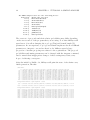
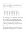
After the initial log likelihoods, MrBayes will print the state of the chains every
100th generation, like this:
Chain results:
100
200
300
400
500
600
700
800
900
1000
0 -- (-7515.474) (-7815.502) (-7571.894) [-7511.216] * (-7912.443) (-7430.324) (-7722.968) [-7559.768]
-- (-6457.486) (-6443.204) (-6362.653) [-6380.948] * (-6452.131) (-6412.384) (-6460.409) [-6335.541] --- (-6372.894) (-6284.653) [-6212.481] (-6320.671) * (-6326.804) [-6206.832] (-6368.248) (-6274.370) --- (-6215.251) (-6238.351) [-6173.761] (-6215.648) * [-6175.548] (-6162.354) (-6295.342) (-6170.237) --- (-6169.260) [-6106.352] (-6157.140) (-6134.522) * [-6044.984] (-6105.105) (-6239.651) (-6126.382) --- (-6132.093) [-6045.345] (-6071.921) (-6105.350) * [-6027.764] (-6052.897) (-6122.643) (-6054.535) --- (-6086.736) [-5966.605] (-6022.943) (-6048.775) * (-6005.907) (-6050.838) (-6052.809) [-5987.512] --- (-6071.156) [-5949.411] (-6001.893) (-6028.975) * (-5969.434) (-6034.590) (-5985.207) [-5962.131] --- (-6043.289) [-5919.917] (-5955.320) (-5990.842) * (-5934.204) (-5998.712) [-5917.514] (-5957.886) --- (-6036.192) [-5915.292] (-5940.829) (-5928.622) * (-5916.117) (-5974.419) [-5885.179] (-5947.285) --- (-6033.926) [-5879.274] (-5930.137) (-5912.750) * (-5919.677) (-5979.409) [-5849.042] (-5893.568) --
0:00:00
0:01:39
0:01:05
0:01:38
0:01:18
0:01:04
0:01:22
0:01:12
0:01:03
0:01:16
Average standard deviation of split frequencies: 0.000000
1100 -- (-6015.382) (-5879.918) (-5932.478) [-5850.292] * (-5845.497) (-5970.688) [-5835.631] (-5882.916) -- 0:01:08
...
19000 -- (-5725.208) (-5728.059) (-5723.771) [-5720.516] * (-5725.163) (-5733.313) (-5731.771) [-5733.018] -- 0:00:03
Average standard deviation of split frequencies: 0.000000
19100
19200
19300
19400
19500
19600
19700
19800
19900
----------
(-5721.777)
(-5725.644)
(-5722.932)
(-5722.253)
[-5723.923]
(-5731.034)
(-5738.424)
(-5732.570)
(-5724.326)
(-5731.432)
[-5723.736]
(-5727.877)
(-5732.094)
(-5732.401)
(-5729.754)
(-5731.187)
(-5732.026)
(-5728.367)
[-5724.683]
(-5730.977)
(-5729.790)
(-5733.256)
(-5726.903)
(-5732.244)
(-5728.800)
(-5729.572)
[-5725.441]
(-5719.899)
(-5718.788)
[-5719.233]
[-5721.040]
(-5722.455)
[-5725.747]
[-5728.881]
[-5727.604]
(-5726.584)
*
*
*
*
*
*
*
*
*
(-5724.676)
[-5732.428]
[-5728.970]
(-5731.382)
(-5727.740)
(-5725.214)
(-5725.340)
[-5721.525]
(-5723.621)
[-5725.091]
(-5725.226)
(-5732.444)
[-5726.897]
(-5722.413)
(-5722.015)
[-5720.537]
(-5718.952)
(-5730.548)
(-5728.996)
(-5733.051)
(-5730.074)
(-5734.551)
(-5736.126)
(-5733.053)
(-5734.678)
(-5741.802)
(-5746.447)
(-5742.658)
(-5741.748)
(-5731.851)
(-5733.469)
[-5727.055]
[-5723.926]
(-5725.685)
(-5722.740)
[-5716.807]
----------
0:00:03
0:00:02
0:00:02
0:00:02
0:00:01
0:00:01
0:00:01
0:00:00
0:00:00
2.2. THOROUGH VERSION
25
20000 -- (-5723.983) (-5727.877) [-5724.582] (-5720.923) * (-5730.172) (-5728.091) (-5748.344) [-5716.947] -- 0:00:00
Average standard deviation of split frequencies: 0.000520
Continue with analysis? (yes/no): no
If you have the terminal window wide enough, each generation of the chain will
print on a single line.
The first column lists the generation number. The following four columns with
negative numbers each correspond to one chain in the first run. Each column
represents one physical location in computer memory, and the chains shift
positions in the columns as the run proceeds (it is actually only the temperature
that is shifted). The numbers are the log likelihood values of the chains. The
chain that is currently the cold chain has its value surrounded by square brackets,
whereas the heated chains have their values surrounded by parentheses. When
two chains successfully change states, they trade column positions (places in
computer memory). If the Metropolis coupling works well, the cold chain should
move around among the columns; this means that the cold chain successfully
swaps states with the heated chains. If the cold chain gets stuck in one of the
columns, then the heated chains are not successfully contributing states to the
cold chain, and the Metropolis coupling is inefficient. The analysis may then
have to be run longer. You can also try to reduce the temperature di↵erence
between chains, which may increase the efficiency of the Metropolis coupling.
The star column separates the two di↵erent runs. The last column gives the time
left to completion of the specified number of generations. This analysis
approximately takes 1 second per 100 generations. Because di↵erent moves are
used in each generation, the exact time varies somewhat for each set of 100
generations, and the predicted time to completion will be unstable in the
beginning of the run. After a while, the predictions will become more accurate
and the estimated remaining time will decrease more evenly between generations.
2.2.7
When to Stop the Analysis
At the end of the run, MrBayes asks whether or not you want to continue with
the analysis. Before answering that question, examine the average standard
26
CHAPTER 2. TUTORIAL: A SIMPLE ANALYSIS
deviation of split frequencies. As the two runs converge onto the stationary
distribution, we expect the average standard deviation of split frequencies to
approach zero, reflecting the fact that the two tree samples become increasingly
similar. In our case, the average standard deviation is down to 0.0 already after
1,000 generations and then stays at very low values throughout the run. Your
values can di↵er slightly because of stochastic e↵ects but should show a similar
trend.
In larger and more difficult analyses, you will typically see the standard deviation
of split frequencies come down much more slowly towards 0.0; the standard
deviation can even increase temporarily, especially in the early part of the run. A
rough guide is that an average standard deviation below 0.01 is very good
indication of convergence, while values between 0.01 and 0.05 may be adequate
depending on the purpose of your analysis. The sumt command (see below)
allows you to examine the error (standard deviation) associated with each clade
in the tree. Typically, most of the error is associated with clades that are not
very well supported (posterior probabilities well below 0.95), and getting
accurate estimates of those probabilities may not be an important depending on
the purpose of the analysis.
Given the extremely low value of the average standard deviation at the end of
the run, there appears to be no need to continue the analysis beyond 20,000
generations so when MrBayes asks Continue with analysis? (yes/no): stop
the analysis by typing no.
Although we recommend using a convergence diagnostic, such as the standard
deviation of split frequencies, there are also simpler but less powerful methods of
determining when to stop the analysis. The simplest technique is to examine the
log likelihood values (or, more exactly, the log probability of the data given the
parameter values) of the cold chain, that is, the values printed to screen within
square brackets. In the beginning of the run, the values typically increase rapidly
(the absolute values decrease, since these are negative numbers). In our case, the
values increase from below 7500 to around 5725 in the first few thousand
generations. This is the ”burn-in” phase and the corresponding samples are
typically discarded. Once the likelihood of the cold chain stops to increase and
starts to randomly fluctuate within a more or less stable range, the run may have
2.2. THOROUGH VERSION
27
reached stationarity, that is, it may be producing a good sample from the
posterior probability distribution. At stationarity, we also expect di↵erent,
independent runs to sample similar likelihood values. Trends in likelihood values
can be deceiving though; you’re more likely to detect problems with convergence
by comparing split frequencies than by looking at likelihood trends.
When you stop the analysis, MrBayes will print several types of information
useful in optimizing the analysis. This is primarily of interest if you have
difficulties in obtaining convergence, which is unlikely to happen with this
analysis. We give a few tips on how to improve convergence at the end of the
following section.
2.2.8
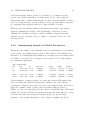
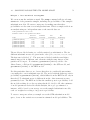
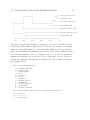
Summarizing Samples of Model Parameters
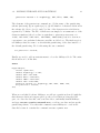
During the run, samples of the substitution model parameters have been written
to the .p files every samplefreq generation. These files are tab-delimited text
files that look something like this (numbers are actually given in scientific format
by default, so the files do not look quite as nice as the one below although they
are structurally equivalent):
[ID: 9409050143]
Gen
LnL
1
-7821.374
100
-6328.159
....
19900
-5723.107
20000
-5720.765
TL
2.100
2.091
r(A<->C)
0.166667
0.166667
...
...
...
pi(T)
0.250000
0.307263
alpha
0.500000
0.842091
pinvar
0.000000
0.036693
2.990
2.959
0.048609
0.048609
...
...
0.251888
0.240826
0.605319
0.636716
0.152817
0.180024
The first number, in square brackets, is a randomly generated ID number that
lets you identify the analysis from which the samples come. The next line
contains the column headers, and is followed by the sampled values. From left to
right, the columns contain: (1) the generation number (Gen); (2) the log
likelihood of the cold chain (LnL); (3) the total tree length (the sum of all branch
lengths, TL); (4) the six GTR rate parameters (r(A<->C), r(A<->G) etc); (5) the
four stationary nucleotide frequencies (pi(A), pi(C) etc); (6) the shape
parameter of the gamma distribution of rate variation (alpha); and (7) the
28
CHAPTER 2. TUTORIAL: A SIMPLE ANALYSIS
proportion of invariable sites (pinvar). If you use a di↵erent model for your data
set, the .p files will of course be di↵erent.
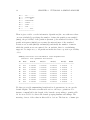
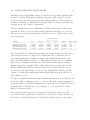
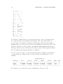
MrBayes provides the sump command to summarize the sampled parameter
values. By default, the sump command uses the same burn-in as the convergence
diagnostics in the mcmc command. This should be appropriate if we use these
diagnostics to determine when we have an appropriate sample from the posterior.
Thus, we can summarize the information in the .p file by simply typing sump.
By default, sump will summarize the information in the .p file or files generated
most recently, but the filename can be changed if necessary. The relburnin=yes
option specifies that we want to give the burn-in in terms of a fraction (relative
burn-in) rather than as an absolute value. The burninfrac option specifies the
desired burn-in fraction.
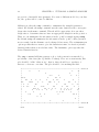
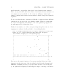
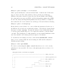
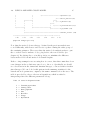
The sump command will first generate a plot of the generation versus the log
probability of the data (the log likelihood values). If we are at stationarity, this
plot should look like ”white noise”, that is, there should be no tendency of
increase or decrease over time. The plot should look something like this:
+------------------------------------------------------------+ -5717.71
|
2
1
1
2|
|
1
1
|
|
2 2
1
1
1 |
|22 2
1
12
1
|
|
22
2
1
1
1
2 1 1
1
2
|
|11
1111
1
1
112
1
2
12
1
|
| 1
*
22
2
1
1*
2
2 |
| 2 1 1
1
1 2*
12
2
12
1
|
|
221 2
12 2
* 2
2
2 1
2
1|
|
2
1 2 *
2
1
1 2 2 2 2
1 |
|
1
1
2 2 11
1
|
|
2 2
2
2
2
12 2 |
|
2
2
|
|
2
|
|
1
1
2
|
+------+-----+-----+-----+-----+-----+-----+-----+-----+-----+ -5731.34
^
^
5000
20000
2.2. THOROUGH VERSION
29
If you see an obvious trend in your plot, either increasing or decreasing, you very
likely need to run the analysis longer to get an adequate sample from the
posterior probability distribution.
At the bottom of the sump output, there is a table summarizing the samples of
the parameter values:
95% HPD Interval
-------------------Parameter
Mean
Variance
Lower
Upper
Median
PSRF+
-----------------------------------------------------------------------------TL
2.925036
0.067504
2.415013
3.379712
2.928130
0.997
r(A<->C)
0.046638
0.000087
0.025996
0.061754
0.047223
1.033
r(A<->G)
0.472949
0.001944
0.380185
0.538198
0.475733
1.093
r(A<->T)
0.038436
0.000070
0.024704
0.057508
0.037291
1.067
r(C<->G)
0.028027
0.000145
0.005312
0.049157
0.028217
1.023
r(C<->T)
0.394395
0.001729
0.319370
0.473755
0.390730
1.110
r(G<->T)
0.019556
0.000169
0.000078
0.044754
0.017799
1.018
pi(A)
0.355732
0.000173
0.333218
0.383760
0.354468
1.064
pi(C)
0.317528
0.000128
0.299947
0.342945
0.317121
1.031
pi(G)
0.082920
0.000045
0.072361
0.096352
0.082537
1.164
pi(T)
0.243820
0.000085
0.224679
0.260468
0.244298
1.014
alpha
0.693416
0.065342
0.336440
1.174297
0.655553
1.061
pinvar
0.165968
0.009690
0.001575
0.310722
0.178146
1.090
------------------------------------------------------------------------------
For each parameter, the table lists the mean and variance of the sampled values,
the lower and upper boundaries of the 95 % credibility interval, and the median
of the sampled values. The parameters are the same as those listed in the .p files:
the total tree length (TL), the six reversible substitution rates (r(A<->C),
r(A<->G), etc), the four stationary state frequencies (pi(A), pi(C), etc), the
shape of the gamma distribution of rate variation across sites (alpha), and the
proportion of invariable sites (pinvar). Note that the six rate parameters of the
GTR model are given as proportions of the rate sum (the Dirichlet
parameterization). This parameterization has some advantages in the Bayesian
context; in particular, it allows convenient formulation of priors. If you want to
scale the rates relative to the G-T rate, just divide all rate proportions by the
G-T rate proportion.
The last column in the table contains a convergence diagnostic, the Potential
Scale Reduction Factor (PSRF). If we have a good sample from the posterior
probability distribution, these values should be close to 1.0. A reasonable goal
might be to aim for values between 1.00 and 1.02 but it can be difficult to
achieve this for all parameters in the model in larger and more complicated
30
CHAPTER 2. TUTORIAL: A SIMPLE ANALYSIS
analyses. In our case, we can probably easily obtain more accurate estimates by
running the analysis slightly longer.
2.2.9
Summarizing Tree Samples
Trees and branch lengths are printed to the .t files. These files are
Nexus-formatted tree files with a structure like this (the real files have branch
lengths printed in scientific format so they look slightly more messy but the
structure is the same):
#NEXUS
[ID: 9409050143]
[Param: tree]
begin trees;
translate
1 Tarsius_syrichta,
2 Lemur_catta,
3 Homo_sapiens,
4 Pan,
5 Gorilla,
6 Pongo,
7 Hylobates,
8 Macaca_fuscata,
9 M_mulatta,
10 M_fascicularis,
11 M_sylvanus,
12 Saimiri_sciureus;
tree gen.1 = [&U] ((12:0.100000,(((((3:0.100000,4:0.100000):0.100000...
...
tree gen.20000 = [&U] (((((10:0.087647,(8:0.013447,9:0.021186):0.030...
end;
To summarize the tree and branch length information, type sumt relburnin =
yes burninfrac = 0.25. The sumt and sump commands each have separate
burn-in settings so it is necessary to give the burn-in here again. Most MrBayes
settings are persistent and need not be repeated every time a command is
executed but the settings are typically not shared across commands. To make
sure the settings for a particular command are correct, you can always use help
<command> before issuing the command.
2.2. THOROUGH VERSION
31
The sumt command will output, among other things, summary statistics for the
taxon bipartitions, a tree with clade credibility (posterior probability) values,
and a phylogram (if branch lengths have been saved). The output first gives a
key to each partition in the tree sample using dots for the taxa that are on one
side of the partition and stars for the taxa on the other side. For instance, the
14th partition (ID 14) in the output below represents the clade Homo (taxon 3)
and Pan (taxon 4), since there are stars in the third and fourth positions and a
dot in all other positions.
List of taxa in bipartitions:
1
2
3
4
5
6
7
8
9
10
11
12
-------------
Tarsius_syrichta
Lemur_catta
Homo_sapiens
Pan
Gorilla
Pongo
Hylobates
Macaca_fuscata
M_mulatta
M_fascicularis
M_sylvanus
Saimiri_sciureus
Key to taxon bipartitions (saved to file "primates.nex.parts"):
ID -- Partition
-----------------1 -- .***********
2 -- .*..........
3 -- ..*.........
4 -- ...*........
5 -- ....*.......
6 -- .....*......
7 -- ......*.....
8 -- .......*....
9 -- ........*...
10 -- .........*..
11 -- ..........*.
12 -- ...........*
13 -- .......****.
32
CHAPTER 2. TUTORIAL: A SIMPLE ANALYSIS
14 -- ..**........
15 -- ..**********
16 -- .......**...
17 -- ..*********.
18 -- ..*****.....
19 -- ..****......
20 -- ..***.......
21 -- .......***..
------------------
Then it gives a table over the informative bipartitions (the ones with more than
one taxon included), specifying the number of times the partition was sampled
(#obs), the probability of the partition (Probab.), the standard deviation of the
partition frequency (Sd(s)) across runs, the min and max of the standard
deviation across runs (Min(s) and Max(s)) and finally the number of runs in
which the partition was encountered. In our analysis, there is overwhelming
support for a single tree, so all partitions in this tree have a posterior probability
of 1.0.
Summary statistics for informative taxon bipartitions
(saved to file "primates.nex.tstat"):
ID
#obs
Probab.
Sd(s)+
Min(s)
Max(s)
Nruns
---------------------------------------------------------------13
302
1.000000
0.000000
1.000000
1.000000
2
14
302
1.000000
0.000000
1.000000
1.000000
2
15
302
1.000000
0.000000
1.000000
1.000000
2
16
302
1.000000
0.000000
1.000000
1.000000
2
17
302
1.000000
0.000000
1.000000
1.000000
2
18
302
1.000000
0.000000
1.000000
1.000000
2
19
302
1.000000
0.000000
1.000000
1.000000
2
20
302
1.000000
0.000000
1.000000
1.000000
2
21
302
1.000000
0.000000
1.000000
1.000000
2
----------------------------------------------------------------
We then get a table summarizing branch and node parameters, in our case the
branch lengths. The indices in this table refer to the key to partitions. For
instance, length[14] is the length of the branch corresponding to partition ID
14. As we noted above, this is the branch grouping humans and chimps. The
meaning of most of the values in this table is obvious. The last two columns give
2.2. THOROUGH VERSION
33
a convergence diagnostic, the Potential Scale Reduction Factor (PSRF), and the
numnber of runs in which the partition was encountered. The PSRF diagnostic is
the same used for the regular parameter samples, and it should approach 1.0 as
runs converge.
Summary statistics for branch and node parameters
(saved to file "primates.nex.vstat"):
95% HPD Interval
-------------------Parameter
Mean
Variance
Lower
Upper
Median
PSRF+ Nruns
-------------------------------------------------------------------------------------length[1]
0.486115
0.007159
0.349117
0.660632
0.477699
0.997
2
length[2]
0.335038
0.003829
0.222216
0.448005
0.331021
1.008
2
length[3]
0.050689
0.000114
0.033718
0.072349
0.049417
1.001
2
length[4]
0.060501
0.000144
0.039651
0.082690
0.060417
0.997
2
length[5]
0.057754
0.000183
0.031723
0.081064
0.056059
1.001
2
length[6]
0.143419
0.000537
0.100539
0.189667
0.140537
1.000
2
length[7]
0.172066
0.001072
0.112808
0.233264
0.172907
1.007
2
length[8]
0.016107
0.000031
0.005941
0.026377
0.015679
1.001
2
length[9]
0.023164
0.000045
0.011955
0.037226
0.022580
0.999
2
length[10]
0.056704
0.000147
0.033104
0.079370
0.056479
0.999
2
length[11]
0.069330
0.000366
0.029295
0.103081
0.070148
1.012
2
length[12]
0.433951
0.005270
0.305526
0.572054
0.426316
0.998
2
length[13]
0.248133
0.002680
0.148162
0.338245
0.243948
0.997
2
length[14]
0.029261
0.000142
0.008043
0.052766
0.028329
0.997
2
length[15]
0.273555
0.003600
0.163707
0.403779
0.268913
1.011
2
length[16]
0.035972
0.000125
0.016521
0.059122
0.035263
0.998
2
length[17]
0.118515
0.001761
0.044026
0.199364
0.119746
0.998
2
length[18]
0.124953
0.001162
0.052839
0.178939
0.122538
0.997
2
length[19]
0.057618
0.000424
0.017331
0.091541
0.057151
1.000
2
length[20]
0.082425
0.000486
0.051259
0.137057
0.080014
0.997
2
length[21]
0.049766
0.000398
0.018269
0.094330
0.047661
0.997
2
--------------------------------------------------------------------------------------
This table is followed by two trees. The clade credibility tree (upper tree) gives
the probability of each partition or clade in the tree, and the phylogram (lower
tree) gives the branch lengths measured in expected substitutions per site:
Clade credibility values:
/--------------------------------------------------------|
|--------------------------------------------------------|
|
/-------|
/--100--+
|
|
\-------|
/--100--+
|
|
\---------------|
/---100--+
+
|
\-----------------------|
/--100--+
|
|
\--------------------------------|
|
|
|
/-------|
/--100--+
/--100--+
|
|
|
|
\--------
Tarsius_syrichta (1)
Lemur_catta (2)
Homo_sapiens (3)
Pan (4)
Gorilla (5)
Pongo (6)
Hylobates (7)
Macaca_fuscata (8)
M_mulatta (9)
34
CHAPTER 2. TUTORIAL: A SIMPLE ANALYSIS
|
|
|
/--100--+
|
|
|
|
\---------------- M_fascicularis (10)
\--100--+
\-------100------+
|
\------------------------ M_sylvanus (11)
|
\------------------------------------------------- Saimiri_sciureus (12)
Phylogram (based on average branch lengths):
/--------------------------------------- Tarsius_syrichta (1)
|
|--------------------------- Lemur_catta (2)
|
|
/---- Homo_sapiens (3)
|
/-+
|
| \----- Pan (4)
|
/------+
|
|
\---- Gorilla (5)
|
/---+
+
|
\------------ Pongo (6)
|
/--------+
|
|
\------------- Hylobates (7)
|
|
|
|
/-- Macaca_fuscata (8)
|
/---------+
/-+
|
|
|
| \-- M_mulatta (9)
|
|
|
/---+
|
|
|
|
\---- M_fascicularis (10)
\--------------------+
\-------------------+
|
\------ M_sylvanus (11)
|
\---------------------------------- Saimiri_sciureus (12)
|--------------| 0.200 expected changes per site
In the background, the sumt command creates five additional files. The first is a
.parts file, which contains the key to taxon bipartitions. The second and third
are the .tstat and .vstat files, which contain the summaries of partition
statistics and branch length statistics, respectively.
The next is the .con file, which includes the consensus trees. By default, the
consensus tree with all the relevant clade support values and branch length
information is printed in a format suitable for FigTree. Once the .con file is
opened in FigTree, you can display statistics such as the posterior probability
and its associated standard deviation on each clade in the tree.
2.2. THOROUGH VERSION
35
Alternatively, you can specify conformat=simple to get the consenus trees in a
simpler format that can be opened in most tree drawing programs. The simple
format contains two di↵erent trees, one with both branch lengths and support
values, and one with only branch lengths. Be sure to select the appropriate one if
you wish to display both branch lengths and support values.
The last file generated by the sumt command is the .trprobs file, which contains
the trees that were found during the MCMC search, sorted by posterior
probability. This allows you to examine the trees contained in various credible
sets of trees. For instance, the 95 % credible set contains the most probable trees
up to an accumulated posterior probability of 95 %. In our case, this file will
only contain one tree, but data sets with more topological uncertainty can
produce long lists of trees in the .trprobs files.
36
CHAPTER 2. TUTORIAL: A SIMPLE ANALYSIS
Chapter 3
Tutorial: A Partitioned Analysis
MrBayes handles a wide variety of data types and models, as well as any mix of
these models. In this example we will look at how to set up a simple analysis of a
combined data set, consisting of data from four genes and morphology for 30
taxa of gall wasps and outgroups. A similar approach can be used, e.g., to set up
a partitioned analysis of molecular data coming from di↵erent genes. The data
set for this tutorial is found in the file cynmix.nex.
3.1
Getting Mixed Data into MrBayes
First, open up the Nexus data file in a text editor. The DATA block of the
Nexus file should look familiar but there are some di↵erences compared to the
primates.nex file in the format statement:
Format datatype=mixed(Standard:1-166,DNA:167-3246)
interleave=yes gap=- missing=?;
First, the datatype is given as mixed followed by a specification of the content of
the matrix: it contains standard (morphology) characters in columns 1-166 and
DNA characters in the remaining columns. The mixed datatype is an extension
to the Nexus standard, which originated in MrBayes 3. It may not be compatible
with other phylogenetics programs.
37
38
CHAPTER 3. TUTORIAL: A PARTITIONED ANALYSIS
Second, the matrix is specified to be interleaved. It is often convenient to specify
mixed data in interleaved format, with each block consisting of a natural subset
of the matrix, such as the morphological data or one of the gene regions.
3.2
Dividing the Data into Partitions
By default, MrBayes partitions the data according to data type. There are only
two data types in the matrix, so the default model will include only a
morphology (standard) and a DNA partition. To divide the DNA partition into
gene regions or other appropriate subsets, it is convenient to first specify
character sets. In principle, this can be done from the command line but it is
easier to do it in a MrBayes block in the data file. With the MrBayes
distribution, we added a file cynmix-run.nex with a complete MrBayes block.
For this section, we are going to create a command block from scratch, but you
can consult the cynmix-run.nex for reference.
In your favorite text editor, create a new file called cynmix-command.nex in the
same directory as the cynmix.nex file and add the following new MrBayes block
(note that each line must be terminated by a semicolon):
#NEXUS
begin mrbayes;
execute cynmix.nex;
charset morphology = 1-166;
charset COI = 167-1244;
charset EF1a = 1245-1611;
charset LWRh = 1612-2092;
charset 28S = 2093-3246;
The first line is required to comply with the nexus standard. With the execute
command, we load the data from the cynmix.nex file and the charset command
simply associates a name with a set of characters. For instance, the character set
COI is defined above to include characters 167 to 1244. The next step is to define
a partition of the data according to genes and morphology. This is accomplished
with the line (add it after the lines above):
3.2. DIVIDING THE DATA INTO PARTITIONS
39
partition favored = 5: morphology, COI, EF1a, LWRh, 28S;
The elements of the partition command are: (1) the name of the partitioning
scheme (favored); (2) an equal sign (=); (3) the number of character divisions in
the scheme (5); (4) a colon (:); and (5) a list of the characters in each division,
separated by commas. The list of characters can simply be an enumeration of the
character numbers (the above line is equivalent to partition favored = 5:
1-166, 167-1244, 1245-1611, 1612-2092, 2093-3246;) but it is often more
convenient to use predefined character sets like we did above. The final step is to
tell MrBayes that we want to work with this partitioning of the data instead of
the default partitioning. We do this using the set command:
set partition = favored;
Finally, we need to add an end statement to close the MrBayes block. The entire
file should now look like this:
#NEXUS
begin mrbayes;
execute cynmix.nex;
charset morphology = 1-166;
charset COI = 167-1244;
charset EF1a = 1245-1611;
charset LWRh = 1612-2092;
charset 28S = 2093-3246;
partition favored = 5: morphology, COI, EF1a, LWRh, 28S;
set partition = favored;
end;
When we read this block into MrBayes, we will get a partitioned model with the
first character division being morphology, the second division being the COI
gene, etc. Save the data file, exit your text editor, and finally launch MrBayes
and type execute cynmix-command.nex to read in your data and set up the
partitioning scheme. Note that this command causes MrBayes to read in the
data file because it contains the command execute cynmix.nex.
40
CHAPTER 3. TUTORIAL: A PARTITIONED ANALYSIS
3.3
Specifying a Partitioned Model
Before starting to specify the partitioned model, it is useful to examine the
default model. Type showmodel and you should get this table as part of the
output:
Active parameters:
Partition(s)
Parameters
1 2 3 4 5
-----------------------------Statefreq
1 2 2 2 2
Ratemultiplier
3 3 3 3 3
Topology
4 4 4 4 4
Brlens
5 5 5 5 5
------------------------------
There is a lot of other useful information in the output of showmodel but this
table is the key to the partitioned model. We can see that there are five
partitions in the model and five active (free) parameters. There are two
stationary state frequency parameters, one for the morphological data
(parameter 1) and one for the DNA data (parameter 2). Then there is also a
ratemultiplier (3), a topology parameter (4) and a set of branch length
parameters (5). All three are the same for all partitions.
Now, assume we want a separate GTR + + I model for each gene partition.
All the parameters should be estimated separately for the individual genes.
Assume further that we want the overall evolutionary rate to be (potentially)
di↵erent across partitions, and that we want to assume gamma-shaped rate
variation for the morphological data. We can obtain this model by using lset
and prset with the applyto mechanism, which allows us to apply the settings to
specific partitions. For instance, to apply a GTR + + I model to the molecular
partitions, we type lset applyto=(2,3,4,5) nst=6 rates=invgamma. This
will produce the following table when showmodel is invoked:
Active parameters:
Partition(s)
3.3. SPECIFYING A PARTITIONED MODEL
41
Parameters
1 2 3 4 5
-----------------------------Revmat
. 1 1 1 1
Statefreq
2 3 3 3 3
Shape
. 4 4 4 4
Pinvar
. 5 5 5 5
Ratemultiplier
6 6 6 6 6
Topology
7 7 7 7 7
Brlens
8 8 8 8 8
------------------------------
As you can see, all molecular partitions now evolve under the correct model but
all parameters (statefreq, revmat, shape, pinvar) are shared across partitions.
To unlink them such that each partition has its own set of parameters, type:
unlink statefreq=(all) revmat=(all) shape=(all) pinvar=(all). Gamma-shaped
rate variation for the morphological data is enforced with lset applyto=(1)
rates=gamma. The trickiest part is to allow the overall rate to be di↵erent
across partitions. This is achieved using the ratepr parameter of the prset
command. By default, ratepr is set to fixed, meaning that all partitions have
the same overall rate. By changing this to variable, the rates are allowed to vary
under a flat Dirichlet prior. To allow all our partitions to evolve under di↵erent
rates, type prset applyto=(all) ratepr=variable.
The model is now essentially complete but there is one final thing to consider.
Typically morphological data matrices do not include all types of characters.
Specifically, morphological data matrices do not usually include any constant
(invariable) characters. Sometimes, autapomorphies are not included either, and
the matrix is restricted to parsimony-informative characters. For MrBayes to
calculate the probability of the data correctly, we need to inform it of this
ascertainment (coding) bias. By default, MrBayes assumes that standard data
sets include all variable characters but no constant characters. If necessary, one
can change this setting using lset coding. We will leave the coding setting at
the default, though, which is variable for standard (morphology) data. Now,
showmodel should produce this table:
Active parameters:
Partition(s)
42
CHAPTER 3. TUTORIAL: A PARTITIONED ANALYSIS
Parameters
1 2 3 4 5
-----------------------------Revmat
. 1 2 3 4
Statefreq
5 6 7 8 9
Shape
10 11 12 13 14
Pinvar
. 15 16 17 18
Ratemultiplier 19 19 19 19 19
Topology
20 20 20 20 20
Brlens
21 21 21 21 21
------------------------------
3.4
Running the Analysis
When the model has been completely specified, we can proceed with the analysis
essentially as described above in the tutorial for the primates.nex data set.
However, in the case of the cynmix.nex dataset, the analysis will have to be run
longer before it converges.
When looking at the parameter samples from a partitioned analysis, it is useful
to know that the names of the parameters are followed by the character division
(partition) number in curly braces. For instance, pi(A){3} is the stationary
frequency of nucleotide A in character division 3, which is the EF1a division in
the above analysis.
In this section we have used a separate Nexus file for the MrBayes block.
Although one can add this command block to the data file itself, there are
several advantages to keeping the commands and the data blocks separate. For
example, one can create a set of di↵erent analyses with di↵erent parameters in
separate command files and submit all those files to a job scheduling system on a
computer cluster. It is important to remember, though, that MrBayes uses the
name of the file containing the character matrix as the default for all output files.
Thus, if you run all your analyses in the same directory, results from di↵erent
analyses will overwrite each other.
To change this behavior, include the command mcmcp
filename=<filename>; in each of your run files, just before issuing the mcmc
command, using a di↵erent file name for each run file. For instance, if you wish
3.4. RUNNING THE ANALYSIS
43
to name the output files from one analysis using the root analysis1, you use the
line mcmcp filename=analysis;. The files will then be named
analysis1.run1.t, analysis1.run2.t, etc. An alternative approach is to run
each analysis in a separate directory, in which case the naming of the output files
will not be an issue.
44
CHAPTER 3. TUTORIAL: A PARTITIONED ANALYSIS
Chapter 4
More Tutorials
In this chapter, we provide a number of brief tutorials that cover a wide range of
common models and analyses in MrBayes. We use a slightly di↵erent format for
these tutorials. First, we assume that you are familiar with the basic working of
the program, so we skip uninteresting details when they should be obvious. Also,
in addition to the conventions used previously, we will often simply give the
command line, including the MrBayes > prompt. What you need to type in is
simply the text after the prompt.
You may wish to start each tutorial by switching o↵ warnings and asking
MrBayes to quietly finish each analysis after the requested number of
generations, without asking you if you want to extend the analysis. You can
accomplish this with the command line:
MrBayes > set autoclose=yes nowarn=yes
The tutorials are largely independent of each other, so it should be possible to
skip directly to a tutorial that is of particular interest. However, some tutorials
form a natural sequence of successively more advanced analyses of the same data
set, so following all of the tutorials in order should give some added insight.
The tutorials by no means cover the entire range of models or analytical options
supported by MrBayes. In chapters 5 and 6 we describe all component models
and algorithms that are available, so refer to these for complete coverage. A
45
46
CHAPTER 4. MORE TUTORIALS
graphical overview of the models implemented in MrBayes 3.2 is provided in
Appendix A.
4.1
An Amino Acid Analysis
In this tutorial, we will explore a couple of di↵erent approaches to amino acid
analyses. First, we will ask MrBayes to integrate over a predetermined set of
fixed rate matrices, and then we will repeat the analysis using a fixed rate
matrix. To start the tutorial, first read in the amino acid data:
MrBayes > execute avian_ovomucoids.nex
To ask MrBayes to sample across fixed amino acid rate matrices, we use the
prset command:
MrBayes > prset aamodelpr = mixed
Now we run the analysis as usual. The analysis is much slower than a normal
nucleotide analysis, so let us try first and see if we can get convergence without
using Metropolis coupling (heated chains). We do this by asking for a single
chain per analysis using nchains = 1 in the mcmc command. Although
convergence might be slightly slower if measured in terms of the number of
generations, the analysis will run much faster without the overhead of the heated
chains. We are still using the default of two parallel runs, so we can monitor
topological convergence on the fly. For the dataset in this tutorial, our results
indicate that about 300,000 generations are sufficient for decent topological
convergence. Run 300,000 generations without heating using the command:
MrBayes > mcmc nchains = 1 ngen = 300000
Now we can summarize the parameter and tree samples as usual using the sumt
and sump commands. The output of the sumt command will include a table
giving the posterior probabilities of the amino acid models:
Model probabilities above 0.050
Estimates saved to file "avian_ovomucoids.nex.mstat".
Model
Posterior
Probability
Standard
Deviation
Min.
Probability
Max.
Probability
4.1. AN AMINO ACID ANALYSIS
47
------------------------------------------------------------------------------aamodel[Jones]
1.000
0.000
1.000
1.000
-------------------------------------------------------------------------------
This particular dataset overwhelmingly supports the Jones model, so this may be
the only model sampled after the burn-in phase. This means that the move
mechanism trying to change the amino acid model will rarely or ever have its
proposals accepted after the burn-in phase. However, the sample from the
posterior may nevertheless be accurate. To determine whether we have an
appropriate sample from the posterior, we simply compare the model
probabilities across independent runs. The range of probabilities, from minimum
to maximum, across independent analyses is given in the table. In our case, we
have two independent analyses, both of which are putting all of the probability
on the Jones model (both minimum and maximum probabilities are 1.000). This
is good evidence that we have an adequate sample from the posterior, since each
run started with a randomly selected amino acid rate matrix.
If desired, it is possible to run the same data set under another amino acid
model, for instance the Dayho↵ model, by fixing the rate matrix. Do this by
running the analysis with the following commands:
MrBayes > prset aamodelpr=fixed(dayhoff)
MrBayes > mcmc nchains = 1 ngen = 300000
Note that the likelihoods printed to screen during the run are much worse (about
100 log likelihood units lower) than those obtained when we sampled over rate
matrices according to their posterior probabilities. As you will discover, the
analysis will not be much faster per generation if we fix the rate matrix, which
may be somewhat counter-intuitive. The reason is that only a single rate matrix
is used in any one generation of the chain, even if we change the rate matrix
between generations. The e↵ect of sampling across rate matrices on the speed of
convergence is data-dependent. Convergence may be slower or faster when you
mix over rate matrices, depending on the e↵ects of the rate matrices on the
complexity of the posterior.
We end this tutorial by pointing out that protein-coding nucleotide sequences
can also be analyzed using amino acid models in MrBayes. MrBayes simply uses
the specified genetic code to translate the codons to amino acids, generating
48
CHAPTER 4. MORE TUTORIALS
relevant ambiguous amino acid state sets when appropriate, before running the
analysis. For instance, we would run a mixed amino acid model analysis on the
protein-coding viral sequences in the replicase.nex data set using:
MrBayes
MrBayes
MrBayes
MrBayes
4.2
>
>
>
>
execute replicase.nex
lset nucmodel = aa
prset aamodelpr = mixed
mcmc nchains = 1 ngen = 300000
Identifying Positively Selected Sites
The purpose of this analysis is to identify positively selected sites in a
protein-coding viral sequence. We will use the data in the file replicase.nex.
First, we read in the data:
MrBayes > execute replicase.nex
Then we specify that we want to use a codon model with omega variation across
sites, and that we want MrBayes to report positive selection probabilities and
site omega values (dN/dS ratios).
MrBayes > lset nucmodel = codon omegavar = ny98
MrBayes > report possel = yes siteomega = yes
This is going to be a slow analysis, so we will run relatively short analyses and
will therefore reset the sampling frequency and the frequency with which we
print to screen to once every 20 generations, so that we can monitor the run
adequately and get more samples than we would otherwise. In the same vein, we
will increase the frequency with which we calculate convergence diagnostics to
once every 500 generations. Even though it is possible to speed up the analysis
by running it without Metropolis coupling, our results indicate that the mixing
across model parameters benefits considerably from the heated chains in this
case, so we will not attempt that. Our results indicate that it is possible to get
decent if not perfect convergence within about 10,000 generations, so let us try
that:
4.2. IDENTIFYING POSITIVELY SELECTED SITES
49
MrBayes > mcmcp printfreq = 20 samplefreq = 20 diagnfreq=500
MrBayes > mcmc ngen = 10000
Now we examine the parameter samples by using the sump command. The
output will dominated by a long table summarizing the estimates of the posterior
distributions of the model parameters, including the probabilities of sites being in
the positively selected class, and the weighted site omega values (dN/dS ratios):
95% HPD Interval
-------------------Parameter
Mean
Variance
Lower
Upper
Median
min ESS* avg ESS
PSRF+
----------------------------------------------------------------------------------------------------------TL
4.563947
0.098902
3.852775
5.086475
4.558925
24.35
28.69
1.011
omega(-)
0.086415
0.000079
0.071653
0.099446
0.085985
25.65
33.41
1.002
omega(N)
1.000000
0.000000
1.000000
1.000000
1.000000
NA
NA
NA
omega(+)
1.212074
0.078799
1.000334
1.803710
1.089336
13.25
26.08
1.020
pi(-)
0.848886
0.001521
0.768849
0.908021
0.855780
18.59
21.49
1.000
pi(N)
0.108926
0.001967
0.002585
0.165223
0.117114
4.85
13.43
1.194
pi(+)
0.042188
0.002153
0.000444
0.152103
0.023432
4.00
44.72
1.131
pi(AAA)
0.012023
0.000007
0.006097
0.014923
0.012476
13.35
22.25
1.005
pi(AAC)
0.015588
0.000011
0.011123
0.021896
0.014725
4.48
16.95
1.006
pi(AAG)
0.018310
0.000023
0.010587
0.028169
0.018029
20.57
167.06
1.087
...
pr+(1,2,3)
0.031105
0.001769
0.000193
0.128472
0.012165
3.84
40.87
1.161
pr+(4,5,6)
0.007634
0.000092
0.000042
0.027822
0.003308
4.67
24.37
1.078
pr+(7,8,9)
0.206222
0.060969
0.001249
0.798449
0.090067
3.24
47.63
1.184
...
omega(1,2,3)
0.593781
0.021720
0.256204
0.844889
0.603819
17.99
30.35
1.198
omega(4,5,6)
0.094908
0.000141
0.072752
0.116642
0.094196
4.39
23.04
1.031
omega(7,8,9)
0.953129
0.002358
0.851367
1.023135
0.964322
30.66
45.53
1.045
...
-----------------------------------------------------------------------------------------------------------
First, note that the e↵ective sample size (ESS) is still somewhat low for many
parameters. The total ESS across the two runs is the double of the average ESS
(avg ESS). The total in this analysis is typically below the recommended
minimum of 100 to 200, so we need to run the analysis longer to get a
publication-quality sample from the posterior. The potential scale reduction
factor (PSRF) also indicates that there is some heterogeneity between the two
independent runs. Nevertheless, the analysis is clearly approaching convergence.
We should not have to run it much longer to get an accurate sample from the
posterior, and we might expect the sample obtained so far to be reasonably close
to the correct values.
Now focus on the summaries of the parameter samples. From the top, the
parameters are total tree length (TL ), the omega values (dN/dS ratios) for the
negatively selected, neutral, and positively selected sites (omega(-) , omega(N) ,
and omega(+) ), the frequencies of the site categories (pi(-) , pi(N) , and pi(+)
), and the stationary state frequencies of the codons (pi(AAA) , pi(AAC) , etc).
The table ends with the probabilities of individual sites being in the positively
50
CHAPTER 4. MORE TUTORIALS
selected class, with pr+(1,2,3) being the probability of the codon corresponding
to nucleotide sites 1–3 being positively selected, pr+(4,5,6) being the
probability for the codon corresponding to sites 4–6 being positively selected, etc.
The positive selection probabilities are followed by the site omega values, which
represent a weighted average for each site across all categories of omega values,
with omega(1,2,3) being the value for the codon corresponding to nucleotide
sites 1–3, omega(4,5,6) the value for the codon corresponding to sites 4–6, etc.
Looking at the values, we note that about 85% (pi(-) ) of the sites are under
strong constraining selection (omega(-) = 0.086 ). Only a small fraction of
sites, around 4%, are under positive selection (pi(+) ). Examination of the
positive selection probabilities and codon site omega values reveals which sites
are most likely to be experiencing positive selection. For instance, the evidence is
strong that site (292,293,294) is under positive selection (pr+(292,293,294) =
0.998 , omega(292,293,294) = 1.21 ).
4.3
Sampling Across the GTR Model Space
A standard approach to Bayesian phylogenetics is to first select an appropriate
substitution model using a model testing approach, such as those implemented in
ModelTest or jModelTest (Posada, 1998, 2008). An alternative, more elegant
approach, is to sample across the substitution model space in the Bayesian
MCMC analysis itself (Huelsenbeck et al., 2004), removing the need for a priori
model testing. The purpose of this tutorial is to demonstrate how to set up an
analysis that integrates out the uncertainty about the correct substitution model
by sampling across the entire general time reversible (GTR) model space. We
will use the data in the file primates.nex .
First, we read in the data:
MrBayes > execute primates.nex
Then we specify that we want to use a gamma model of rate variation across
sites, and that we want to sample across the GTR model space:
4.3. SAMPLING ACROSS THE GTR MODEL SPACE
51
MrBayes > lset nst=mixed rates=gamma
We can now run the analysis as usual. The sump command will give relevant
summaries of the parameter samples, including the probabilities of the sampled
substitution models. We assess convergence by making sure that these
probabilities are the same across independent runs. This is a sample table from
an analysis using two independent runs on the tutorial data set:
Model probabilities above 0.050
Estimates saved to file "primates.nex.mstat".
Posterior
Standard
Min.
Max.
Model
Probability
Deviation
Probability
Probability
---------------------------------------------------------------------------------gtrsubmodel[121123]
0.195
0.033
0.172
0.219
gtrsubmodel[121324]
0.089
0.005
0.086
0.093
gtrsubmodel[121323]
0.079
0.009
0.073
0.086
gtrsubmodel[121321]
0.060
0.037
0.033
0.086
gtrsubmodel[123324]
0.060
0.000
0.060
0.060
gtrsubmodel[121121]
0.053
0.009
0.046
0.060
----------------------------------------------------------------------------------
The models are labeled using a so-called restricted growth function. The six
di↵erent substitution rates are given in the order {rAC , rAG , rAT , rCG , rCT , rGT }.
The first rate is labeled “1”. The next rate is labeled with the next higher,
unused integer if it is di↵erent, and otherwise with the same integer as the
partition it belongs to. For instance, gtrsubmodel[111111] refers to the
Jukes–Cantor or F81 model, gtrsubmodel[123456] to the GTR model, and
gtrsubmodel[121121] to the HKY model.
For this particular data set, we observe that there is considerable uncertainty
concerning the correct substitution model. The model with the highest posterior
probability is gtrsubmodel[121123], which di↵ers from the HKY model only in
that the G–T substitution rate is di↵erent from the other transversion rates,
presumably lower. The HKY model has the smallest posterior probability of all
the models reaching above the reporting threshold of 0.050. All other estimates
of model parameters derived from this analysis, the topology estimate for
instance, will be based on an average across the sampled substitution models,
each one weighted according to its posterior probability.
To assess convergence when you sample across the GTR substitution model
space, focus on the variation across runs in estimated model probabilities. The
52
CHAPTER 4. MORE TUTORIALS
table gives the standard deviation as well as the range of estimated values across
runs. Here, we see some heterogeneity across runs in model probabilities, but
most models receive similar probabilities in the two independent runs.
4.4
Testing a Topological Hypothesis
In this tutorial, we will use Bayes factor comparisons to test a topological
hypothesis, namely that humans are more closely related to chimps than to other
primates. Specifically, we will contrast the hypothesis that humans and chimps
form a monophyletic group (M1 ), with the hypothesis that humans and chimps
do not form a monophyletic group (M2 ). In order to do this, we need to compute
the ratio of the marginal likelihoods of the two models, M1 and M2 . This ratio is
known as the Bayes factor. We will use the data in the file primates.nex for the
analysis.
First, read in the data using:
MrBayes > execute primates.nex
Now let us specify a GTR + I +
model:
> lset nst=6 rates=invgamma
Before we can test the hypothesis, we need to specify a hard constraint and a
negative constraint. The hard constraint will allow us to force a partition to
always be present in the sampled trees. The negative constraint will allow us to
sample across all trees that do not contain the specified partition. Specify the
constraints using the following commands:
MrBayes > constraint humanchimp = Homo_sapiens Pan
MrBayes > constraint nohumanchimp negative = Homo_sapiens Pan
MrBayes provides two methods for estimating marginal model likelihoods. The
first is based on the harmonic mean of the likelihood values of the MCMC
samples. It is simple to compute but it is a pretty rough estimate of the model
likelihood. To obtain a more accurate model likelihood, MrBayes provides the
stepping-stone method First, let us use the harmonic mean estimate of the model
4.4. TESTING A TOPOLOGICAL HYPOTHESIS
53
likelihoods of the two models we want to compare. First we enforce the positive
constraint, run an mcmc analysis with 100,000 generations, and use sump to get
the harmonic mean estimate:
MrBayes > prset topologypr=constraints(humanchimp)
MrBayes > mcmc ngen=100000
MrBayes > sump
In the output from the sum command, focus on the table summarizing the
likelihoods of the MCMC samples:
Estimated marginal likelihoods for runs sampled in files
"primates.nex.run1.p" and "primates.nex.run2.p":
(Use the harmonic mean for Bayes factor comparisons of models)
(Values are saved to the file primates.nex.lstat)
Run
Arithmetic mean
Harmonic mean
-------------------------------------1
-5720.59
-5729.69
2
-5720.75
-5735.25
-------------------------------------TOTAL
-5720.67
-5734.56
-------------------------------------It is the harmonic mean that we will use as the initial estimate of the model
likelihood. The estimate of the logarithm of the model likelihood is 5734.56,
with a little bit of heterogeneity between the runs.
Now we enforce the negative constraint, and repeat the procedure using the
commands:
MrBayes > prset topologypr=constraints(nohumanchimp)
MrBayes > mcmc ngen=100000
MrBayes > sump
Our run produced the following estimates of the log of the model likelihoods:
Run
Arithmetic mean
Harmonic mean
--------------------------------------
54
CHAPTER 4. MORE TUTORIALS
1
-5727.08
-5738.92
2
-5725.67
-5737.63
-------------------------------------TOTAL
-5726.15
-5738.47
--------------------------------------
The harmonic mean estimate for this model is 5738.47 in log units, which is
about 4 log units worse than the previous model. A log di↵erence in the range of
3–5 is typically considered strong evidence in favor of the better model, while a
log di↵erence above 5 is considered very strong evidence (Kass and Raftery,
1995). Thus, the harmonic mean estimator indicates that we have strong
evidence in favor of human and chimp being each others closest relatives, with
Gorilla and other primates being more distant.
It may also be interesting to look at the best estimate of the phylogeny under the
assumption that humans and chimps are not each others sister groups. Do this
by typing sumt. As you will see, this tree groups chimps and gorillas together,
with humans being just outside, as one might have expected.
Let us now repeat the comparison using the more accurate stepping-stone
sampling approach. Instead of using the mcmc command followed by the sump
command, we simply use the ss command instead, which will produce the
estimated model likelihood directly. The stepping-stone analysis moves from the
posterior to the prior through a number of steps in which the sampled
distribution is a mixture of varying proportions of the two.
Ideally, one would like to see evidence of convergence among independent runs in
each of the steps of the stepping-stone sampling algorithm. As the algorithm
moves close to the prior, however, we expect this to be difficult. This will be
especially true for the topology parameter, as the number of trees with similar
probability will become huge for any reasonably-sized set of taxa.
To help you monitor convergence during stepping-stone sampling, MrBayes will
print the average standard deviation of split frequencies across runs if you use at
least two independent, parallel runs. Each step in the algorithm is treated as an
independent MCMC sampling problem. The only burn-in phase used by the
algorithm occurs before the first step of the algorithm. Once the step sampling
4.4. TESTING A TOPOLOGICAL HYPOTHESIS
55
starts, each step simply serves as the burn-in for the next one. The length of the
initial burn-in can be specified either in terms of the number of samples to be
discarded (positive numbers) or in terms of step lengths (negative numbers). By
default, the initial burn-in phase is as long as one of the subsequent steps in the
algorithm, that is, burninss = -1 .
To obtain an adequate sample from most of the steps in the algorithm, we will
use 50 steps (the default) with 5,000 generations each, for a total of 250,000
generations. If we add the initial burn in of 5,000 generations (one step), the
total run length wil be 255,000. To monitor convergence twice during each step,
we set the diagnostics frequency to once every 2,500 generations. Stepping-stone
analysis under the two models using these settings will be generated by the
following commands:
MrBayes
MrBayes
MrBayes
MrBayes
>
>
>
>
prset topologypr=constraints(humanchimp)
ss ngen=250000 diagnfreq=2500
prset topologypr=constraints(nohumanchimp)
ss
The output from the ss command will include the following table, which is
given here for the first model:
Marginal likelihood (in natural log units) estimated using stepping-stone sampling based on
50 steps with 5000 generations (10 samples) within each step.
Run
Marginal likelihood (ln)
----------------------------1
-5788.13
2
-5785.85
----------------------------Mean:
-5786.45
In our run, the second model produced the following version of the same table:
Marginal likelihood (in natural log units) estimated using stepping-stone sampling based on
50 steps with 5000 generations (10 samples) within each step.
Run
Marginal likelihood (ln)
----------------------------1
-5797.09
2
-5798.19
----------------------------Mean:
-5797.50
The model likelihoods are thus 5786.45 for the first model and 5798.19 for the
second (in natural log units). We first note that both likelihoods are considerably
56
CHAPTER 4. MORE TUTORIALS
smaller than the corresponding values based on the harmonic mean estimator.
This is an expected e↵ect due to the reliance of the harmonic mean estimator on
rare samples of very low likelihood. Short runs are unlikely to include such
samples, resulting in the harmonic mean estimator usually being biased upwards
in practice.
We also note that the more accurate model likelihoods suggest a larger di↵erence
between the two models, about 11 log likelihood units. Thus, we conclude that
the better model (humans and chimps do form a monophyletic group) is very
strongly supported by a Bayes factor test.
Finally, let us examine one of the convergence diagnostics plots from one of our
stepping-stone analyses. It will probably look something like this:
Plot of average standard deviation of split frequencies across steps.
Points at -1.0 (y-axis) indicates that there were no splits
above minimum frequency for corresponding step.
+------------------------------------------------------------+ 0.11
|
*
|
|
|
|
*
*
|
|
|
|
|
|
|
|
*
|
|
*
*
*
|
|
*
|
|
*
|
|
*
|
|
* * *
|
|
*
* |
|
*
**
|
|***** **** ***** **** ** * * ** ** *
* **
**|
+------+-----+-----+-----+-----+-----+-----+-----+-----+-----+ 0.07
^
^
1
50
Here, we see the expected pattern of low average standard deviation of split
frequencies in the early steps of the algorithm (to the left in the diagram), and
difficulties of sampling across topology space when we move closer to the prior
(to the right in the diagram). By increasing the length of each step, it should be
4.5. TESTING THE STRICT MOLECULAR CLOCK
57
possible to improve convergence also in the steps close to the prior, and therefore
increase the precision of the estimated model likelihoods. However, the similarity
between the two independent estimates of the model likelihood we obtained in
this analysis suggests that the accuracy is already reasonably good.
4.5
Testing the Strict Molecular Clock
In this tutorial, we will use a Bayes factor comparison to test the strict clock
model against the non-clock model for an example data set, primates.nex. The
data set is unusual in that a standard non-clock analysis suggests that the
evolution of these sequences may be fairly well explained by a strict clock. The
analysis is quite similar to the previous one, so you might find it useful to go
through that tutorial first. The basic idea is that we want to compare the
marginal likelihoods of the two models (non-clock and strict clock) against each
other. To do that we need to estimate the marginal likelihoods either using the
rough harmonic mean method or the more accurate stepping-stone method. We
will use both in this tutorial and compare the results.
As usual, we first read in the data:
> execute primates.nex
Then we specify a GTR + I +
model:
MrBayes > lset nst=6 rates=invgamma
To estimate marginal likelihoods of the two models using harmonic means of the
likelihoods of the MCMC samples, we simply run an ordinary MCMC analysis
and obtain the appropriate values using the standard sump command.
Specifically, we first run the standard non-clock model for 100,000 generations
and summarize the obtained samples using sump :
MrBayes > mcmc ngen=100000
MrBayes > sump
In the sump output, we focus on the table summarizing the means of the
likelihoods of the MCMC samples obtained after the burn-in:
58
CHAPTER 4. MORE TUTORIALS
Run
Arithmetic mean
Harmonic mean
-------------------------------------1
-5720.67
-5735.68
2
-5719.97
-5730.58
-------------------------------------TOTAL
-5720.26
-5734.99
--------------------------------------
The harmonic mean suggests that the marginal likelihood of the standard
non-clock model is 5734 log units. Notice, however, some heterogeneity
between the runs.
Now we repeat the procedure under the strict clock model. To enforce branch
lengths to conform to a strict clock, we choose one of the clock priors for the
branch lengths. Specifically, we are going to use the uniform prior on clock trees.
The other commands are the same as those used previously:
> prset brlenspr=clock:uniform
> mcmc ngen=100000
> sump
Again, we focus on the table summarizing the means of the likelihoods of the
MCMC samples:
Run
Arithmetic mean
Harmonic mean
-------------------------------------1
-5719.69
-5726.23
2
-5719.44
-5733.01
-------------------------------------TOTAL
-5719.55
-5732.32
-------------------------------------The harmonic mean is lower for the strict-clock mode than for the non-clock
model, the log values being 5732 and 5734, respectively. This is as we
suspected, but the di↵erence is small and there is overlap between the estimates
obtained in individual runs. In this case, we undoubtedly need the increased
accuracy of the stepping- stone sampling method.
Before moving on to the stepping-stone analysis, first compute a summary of the
tree samples using the sumt command. Now focus on the phylogram, the second
4.5. TESTING THE STRICT MOLECULAR CLOCK
59
tree, in the output from this command. It should look something like this:
Phylogram (based on median node depths):
/----/-+
| \----/-------+
|
\------/----+
|
\--------------/-------------+
|
\-------------------|
|
/-/----------+
/--+
|
|
| \-|
|
/---+
|
|
|
\----/------------+
\------------------------+
|
|
\--------|
|
+
\--------------------------------------------|
|
/-------------------------------------------\-------------+
\--------------------------------------------
Homo_sapiens (3)
Pan (4)
Gorilla (5)
Pongo (6)
Hylobates (7)
Macaca_fuscata (8)
M_mulatta (9)
M_fascicularis (10)
M_sylvanus (11)
Saimiri_sciure~ (12)
Tarsius_syrichta (1)
Lemur_catta (2)
-|---------|--------|---------|--------|---------|--------|
0.60
0.50
0.40
0.30
0.20
0.10
0.00
[Expected changes per site]
We briefly want to point out two things. First, all tips in the tree have the same
distance to the root in the consensus phylogram, the summary tree that is based
on branch lengths. This is because the default assumption in a strict-clock model
is that the tips are of the same age. This assumption can be altered as shown
below in the tutorial on dating. Second, the clock tree is rooted, unlike a tree
resulting from a non-clock analysis. An unrooted tree is drawn by convention
such that it is rooted on the outgroup taxon. This means that it will have a
basal trichotomy, or a basal polytomy of higher degree if outgroup relationships
are unresolved. The specified outgroup taxon (by default the first taxon in the
matrix) will be the first member lineage of the basal trichotomy. A strict-clock
analysis, however, produces a rooted tree, which should have a dichotomy at the
60
CHAPTER 4. MORE TUTORIALS
root unless there is uncertainty concerning the resolution near the base of the
tree. Such a tree does not have to be artificially rooted for drawing purposes
using an outgroup. Thus, the outgroup setting is irrelevant in analyses of clock
tree models. The outgroup setting is only used when drawing unrooted trees.
Now let us continue with a more accurate assessment of the marginal model
likelihoods using the stepping-stone method. It estimates the model likelihood by
sampling a series of distributions that represent di↵erent mixtures of the
posterior distribution and the prior distribution (Xie et al., 2011). The
stepping-stone algorithm is invoked with the ss command, and it uses the same
computational machinery as the mcmc command for each of the steps. Let us run
the algorithm for 50 steps (the default) of 5,000 generations each, which makes a
total of 250,000 generations. We will adjust the default frequency of calculating
convergence diagnostics to once every 2,500 generations to get two reports from
each step in the algorithm. By default, the algorithm uses an initial burn-in
corresponding to one step, which corresponds to setting the burninss option to
1. The total length of the analysis will therefore be 255,000 generations.
As before, the run needs to be repeated for each of the two models. The
following set of commands will run stepping-stone sampling on the non-clock
model. Note that we first reset the prior on branch lengths to the default, an
independent exponential prior with the rate parameter 10.0. An alternative way
of resetting the model to the default is to execute the data set again. If you
choose that alternative, do not forget to specify the GTR + I + model before
running the stepping-stone method.
> prset brlenspr=unconstrained:exp(10.0)
> ss ngen=255000 diagnfreq=2500
The estimated marginal likelihoods are found in a table printed by the ss
command after the analysis is completed. Here are the estimates from our run:
Run
Marginal likelihood (ln)
--------------------------1
-5791.38
2
-5792.04
---------------------------
4.5. TESTING THE STRICT MOLECULAR CLOCK
Mean:
61
-5791.66
We now run the same analysis on the strict clock model:
> prset brlenspr=clock:uniform
> ss ngen=255000 diagnfreq=2500
We got the following estimates of the marginal model likelihoods:
Run
Marginal likelihood (ln)
--------------------------1
-5774.94
2
-5774.75
--------------------------Mean:
-5774.84
First we note that there is good agreement between the two independent
analyses for both models, indicating that we now have accurate estimates of the
marginal model likelihoods. If we compare these estimates with the harmonic
mean estimates, it is striking that they are both much lower. Although the
harmonic mean estimator is unbiased if you let the number of samples go to
infinity, it relies heavily on rarely sampled states with low likelihood. Short runs
tend not to include such samples, so the harmonic mean estimate is often
considerably inflated in practice.
We also see that the strict-clock model is now almost 17 log likelihood units
better than the non-clock model. A di↵erence exceeding 5 log likelihood units is
usually considered very strong evidence in favor of the better model (Kass and
Raftery, 1995). If you are familiar with likelihood ratio tests, it may seem
counter-intuitive that the strict clock model can be so strongly preferred. After
all, the strict clock is just a special case of the non-clock model, so the likelihood
must necessarily be higher, or at least as high, for the latter. How can the
strict-clock model still be preferred in the Bayes factor test?
The answer has to do with the number of parameters. For a data set with n
taxa, a non-clock model has roughly 2n independent branch length parameters,
whereas a strict clock model only has around n independent node times. The
other model parameters, the ones associated with the topology and the
62
CHAPTER 4. MORE TUTORIALS
substitution model, are so few in comparison to the branch lengths or node times
that they can be neglected. Thus, a strict clock model is much more parsimonious
than a non-clock model in the number of parameters, and in Bayesian model
choice, there is a built-in correction for the number of parameters.
One way of explaining the correction is by noting that comparing marginal
model likelihoods is the same thing as comparing the average likelihood across
the joint prior distribution over all model parameters. By including more
parameters, we are almost always going to increase the peak likelihoods, but
whether the average likelihood increases is a complex function of the distribution
of likelihood values with respect to the joint prior distribution. If the simpler
model already captures values close to the peak likelihoods of the more complex
model, then the latter is likely to have a lower average likelihood when the values
are spread out across its larger parameter space. This is what happens here,
resulting in a strong preference for the strict clock model.
For a brief discussion on convergence diagnostics and the plot printed by the ss
command, see the previous tutorial.
4.6
Using a Relaxed Clock Model
In this analysis, we will set up a relaxed clock model for the same data set,
primates.nex, used in the previous two tutorials. A relaxed clock model is
intermediate between a strict clock model and a non-clock model. It has one or a
few more parameters than a strict clock model, but much fewer than a non-clock
model. Unlike a non-clock model, it produces a rooted tree, but the information
about the position of the root is not as strong as in a non-clock analysis. Because
the information about the position of the root might be weak, it is often
beneficial to add a rooting constraint to a relaxed clock analysis. It can help a
relaxed clock analysis correctly infer rate variation close to the base of the tree,
variation that might otherwise cause rooting artifacts. It can also help speed up
convergence, since it may be difficult for an MCMC analysis to mix adequately
across multiple alternative root positions in a relaxed clock tree; this is going to
be the case for this data set. To speed up convergence, and to show you how to
4.6. USING A RELAXED CLOCK MODEL
63
set up a rooting constraint, we will choose the rooting option for this tutorial.
Specifically, we will accept the common view that lemurs form the sister group of
other primates.
As usual, we first read in the data:
> execute primates.nex
Then we specify a GTR + I +
model:
MrBayes > lset nst=6 rates=invgamma
To specify a rooting constraint, we first need to know the order of the taxa in the
data matrix, or their names. We can do this by looking into the data file or by
printing the matrix using the showmatrix command. In either case, we will
discover that the only lemur in the matrix, Lemur catta, is taxon number 2. To
specify a hard constraint that includes all taxa but taxon 2, we can use the
following command:
MrBayes > constraint ingroup = 1 3-.
The constraint command first gives the name of the constraint, and then the
constraint is specified after the equal sign using a list of taxa, where the taxa can
be specified using either their index in the matrix (1, 2, etc) or their name. A
period is synonymous with the last taxon in the matrix, and a range is indicated
using a dash. By default, the constraint is assumed to be positive or hard, that
is, we wish to enforce the specified split or clade to always be present in the
sampled trees.
To enforce the constraint, we also need to set the topology prior using the
following command:
MrBayes > prset topologypr = constraints(ingroup)
Inside the parenthesis, it is possible to give one or more previously defined
constraints, separated by a comma. We are now ready to specify the relaxed
clock model, which is done in two steps. First, we select an underlying strict
clock model. Let us use the simple uniform clock model, which would be
specified with the command:
64
CHAPTER 4. MORE TUTORIALS
MrBayes > prset brlenspr = clock:uniform
Other options include the coalescent and the birth – death models. In the next
step, we select a model for the variation of the clock rate across lineages.
MrBayes o↵ers three relaxed clock models: the Thorne–Kishino 2002 (TK02),
the compound poisson process (CPP), and the independent gamma rates (IGR)
models. Let us use the independent gamma rates model, which is a continuous
uncorrelated model of rate variation across lineages. We invoke this model using:
MrBayes > prset clockvarpr=igr
Each relaxed clock model has one or more additional parameters. In the case of
the IGR model, it is the rate at which the variance of the e↵ective branch length
increases over time, Igrvarpr . Because the strict clock model fits this data set
so well (see previous tutorial), we do not expect the variance to increase much
over time. The default prior for this parameter, an exponential distribution with
rate 10.0, should be more than generous enough for our analysis.
To check the model settings, it is wise to first run the showmodel command.
Once you are convinced that the model settings are OK, run the analysis for
100,000 generation using:
MrBayes > mcmc ngen=100000
We can now verify using the sumt command that the tree is rooted correctly
and that it looks reasonable. We focus on the phylogram, the second tree to be
displayed:
Phylogram (based on median node depths):
/---------------------------------------------------------|
| /------------------------------------------------------| |
| |
/------| |
/--+
+ |
| \------| |
/-------+
| |
|
\---------| |
/----+
| |
|
\-----------------\--+
/----------+
Lemur_catta (2)
Tarsius_syrichta (1)
Homo_sapiens (3)
Pan (4)
Gorilla (5)
Pongo (6)
4.6. USING A RELAXED CLOCK MODEL
|
|
\----------------------|
|
|
|
/---|
/---------+
/--+
|
|
|
| \---|
|
|
/---+
|
|
|
|
\------\----------+
\----------------------+
|
\----------|
\--------------------------------------------
65
Hylobates (7)
Macaca_fuscata (8)
M_mulatta (9)
M_fascicularis (10)
M_sylvanus (11)
Saimiri_sciure~ (12)
-----|--------|--------|--------|--------|--------|-------|
0.60
0.50
0.40
0.30
0.20
0.10
0.00
[Expected changes per site]
Note that the strict clock tree that we obtained in the previous analysis was
rooted di↵erently, with Lemur and Tarsius together forming the sister group of
the remaining primates. The reason that the strict clock analysis prefers to put
the root there can be understood by going back to the non-clock tree (see
chapter 2). By placing the root in this position, we minimize the di↵erence
between the non-clock and strict clock branch lengths.
If the rooting assumption we are using here is correct, then there must have been
some changes in the evolutionary rate close to the root. Specifically, we should
see a deceleration in the Lemur and Tarsius lineages, or an acceleration in their
sister lineages. We can look for this pattern in the summary statistics for the
branch and node parameters, output by the sumt command before the trees. The
table is preceded by a key to the taxon bipartitions, which is critical to
interpreting where the di↵erent parameters belong:
List of taxa in bipartitions:
1
2
3
4
5
6
7
--------
Tarsius_syrichta
Lemur_catta
Homo_sapiens
Pan
Gorilla
Pongo
Hylobates
66
CHAPTER 4. MORE TUTORIALS
8
9
10
11
12
------
Macaca_fuscata
M_mulatta
M_fascicularis
M_sylvanus
Saimiri_sciureus
Key to taxon bipartitions (saved to file "primates.nex.parts"):
ID -- Partition
-----------------0 -- ************
1 -- *...........
2 -- .*..........
3 -- ..*.........
4 -- ...*........
5 -- ....*.......
6 -- .....*......
7 -- ......*.....
8 -- .......*....
9 -- ........*...
10 -- .........*..
11 -- ..........*.
12 -- ...........*
13 -- ..**........
14 -- *.**********
15 -- ..**********
16 -- .......**...
17 -- .......****.
18 -- ..*****.....
19 -- ..***.......
20 -- ..****......
21 -- ..*********.
22 -- .......***..
-----------------Now let us find the ID of the partitions corresponding to the Lemur and Tarsius
lineages, and their sister lineages. We first identify the taxon ID of Lemur and
find that it is 2. Now we find the partition ID that has a single star in the second
position; it is the bipartition that separates Lemur catta from all other taxa.
Not surprisingly, the bipartition ID is 2. The sister lineage of Lemur catta
4.6. USING A RELAXED CLOCK MODEL
67
includes all taxa except Lemur catta. To find the corresponding bipartition ID,
we need to find the ID that has a partition descriptor with a single dot in the
second position; all other positions should be filled with stars. This bipartition
has ID 14. Similarly, we find that the bipartition IDs of Tarsius syrichta and
its sister lineage are 1 and 15, respectively.
Now we examine the posterior distribution of IGR branch rates for these taxon
bipartitions. If the clock is accelerated, the branch rate should be above 1.0; if
the rate is decelerated, the branch rate should be below 1.0. This is the relevant
rows of the table:
95% HPD Interval
-------------------Parameter
Mean
Variance
Lower
Upper
Median
PSRF+ Nruns
---------------------------------------------------------------------------------------------------Igrbranchlens_rate[1]
0.916002
0.037357
0.545476
1.196117
0.947514
1.002
2
Igrbranchlens_rate[2]
0.688266
0.033214
0.345016
0.946393
0.703381
0.997
2
Igrbranchlens_rate[14]
0.776625
1.237010
0.000000
2.947193
0.424638
1.001
2
Igrbranchlens_rate[15]
2.635028
8.175572
0.634393
6.162516
1.809020
0.997
2
----------------------------------------------------------------------------------------------------
We see that there is considerable uncertainty about the branch rates but some of
our predictions seem to be supported. In particular, the evolutionary rate is
decelerated in the lineage leading to Lemur catta, with bipartition ID 2; the
entire 95% HPD interval is below 1.0. Although the evidence is less compelling,
there is also an indication that the rate is decelerated in the lineage leading to
Tarsius syrichta, bipartition ID 1, and considerably accelerated in its sister
lineage with bipartition ID 15. However, there is no evidence that the rate is
accelerated in the sister lineage of Lemur catta with bipartition ID 14. On the
contrary, both the mean and median indicate that this rate is more likely to be
below than above 1.0.
To help you visualize parameters such as branch rates inferred by a relaxed clock
model, the sumt command produces a .con.tre file that contains summaries of
all branch and node parameter samples in a format that can be displayed by the
program FigTree. This allows you, for instance, to color branches according to
inferred evolutionary rates.
If you performed the Bayes factor comparison between the strict clock and
non-clock models for this data set in the previous tutorial, you may wonder how
the relaxed clock model stacks up. To make the comparison fair, let us compare
68
CHAPTER 4. MORE TUTORIALS
the strict clock and relaxed clock models using the same rooting constraint that
we enforced above. To get an accurate comparison, we run the stepping-stone
sampling method. We refer to the previous two tutorials for details, but briefly
give the commands here for the two stepping-stone analyses that are required for
this comparison:
MrBayes > ss ngen=250000 diagnfreq=2500
MrBayes > prset clockvarpr=strict
MrBayes > ss
The results are summarized in the tables outout by the ss command. The results
we got are summarized below, with the relaxed clock model first, followed by the
strict clock model:
Run
Marginal likelihood (ln)
--------------------------1
-5785.05
2
-5785.76
--------------------------Mean:
-5785.34
...
Run
Marginal likelihood (ln)
--------------------------1
-5780.04
2
-5781.53
--------------------------Mean:
-5780.53
Note that the models are close, but it is still the strict clock model that carries
the day. The di↵erence is almost five log units, which is considered strong
evidence in favor of the better model ??. Our runs indicate that the result is
going to be similar if we were to repeat the comparison without enforcing a
rooting constraint. We end by pointing out that this is a rather unusual data set;
most other data sets will strongly favor relaxed over strict clock models.
4.7. NODE DATING AND TOTAL-EVIDENCE DATING
4.7
69
Node Dating and Total-Evidence Dating
In this tutorial, we will use three di↵erent approaches to dating. First, we will
show how to calibrate a tree based on information about the clock rate (rate
dating), then we will date the tree based on node calibrations (node dating), and
finally we will use total-evidence dating (or tip dating), in which the tree is dated
based on simultaneous analysis of fossil and recent taxa. Rate dating and node
dating will be demonstrated on a small data set, primates.nex, which has been
analyzed in several previous tutorials, while a much larger data set,
hymfossil.nex will be used to demonstrate total-evidence dating and node
dating in a more typical setting.
We begin by reading in the smaller data set using the command
MrBayes > execute primates.nex
Next, we set the substitution model to GTR + I + :
MrBayes > lset nst=6 rates=invgamma
We know from previous tutorials (see sections 4.5 and 4.6) that a strict clock
model provides a good fit to the data set. Specifically, we choose a strict clock
model with uniform branch lengths using the command:
MrBayes > prset brlenspr=clock:uniform
By default, the clock rate is going to be fixed to 1.0, which means that the age of
the nodes in the tree will be measured in terms of the number of expected
substitutions per site. If we want a dated tree, it is sufficient to change this
assumption. For instance, let us assume that we know that the rate is
approximately 0.01 ± 0.005 substitutions per site per million years. To use this
assumption, we could for instance use a normal distribution as the prior for the
clock rate, using 0.02 as the mean and 0.005 as the standard deviation. Since we
give these values using millions of years as the unit, the resulting tree will be
calibrated in millions of years.
Setting the prior on the clock rate is thus achieved with
MrBayes > prset clockratepr = normal(0.01,0.005)
70
CHAPTER 4. MORE TUTORIALS
There is one more thing to consider before we can run the analysis. By default,
the clock rate is fixed to 1.0. This means that the tree age (or height, if you
wish) measured in substitutions per site is the same as tree age measured in time
units. As soon as these two measures are decoupled, it is important to consider
whether the clock tree prior is defined in terms of substitution units or time
units. MrBayes uses clock tree priors that are defined on parameters (speciation
rate, extinction rate etc) measured in time rather than substitution units.
The uniform clock tree prior has only one prior parameter, tree age. The default
prior is an exponential distribution with rate parameter 1.0, which usually works
well as long as the clock rate is fixed to 1.0. When we change the clock prior, we
usually need to reconsider this prior. For instance, we might want to modify the
prior so that it has the same e↵ect on branch lengths measured in substitution
units. In our case, we want to change the default prior, with expected mean 1.0,
to one with expected mean 1.0/0.01 = 100, that is, the original value divided by
the expected clock rate. Since the expectation of the exponential distribution is
the same as the inverse of the rate parameter, we thus need to modify the tree
age prior to an exponential distribution with the rate 0.01. We do this using the
following command line.
MrBayes > prset treeagepr = exponential(0.01)
Now let us run a short MCMC analysis using 100,000 generations and the default
settings. After that, we use the sumt command to examine the calibrated tree:
MrBayes > mcmc ngen=100000
MrBayes > sumt
The resulting dated phylogram should look something like this:
/----/-+
| \----/-------+
|
\------/----+
|
\--------------/-------------+
|
\-------------------|
Homo_sapiens (3)
Pan (4)
Gorilla (5)
Pongo (6)
Hylobates (7)
4.7. NODE DATING AND TOTAL-EVIDENCE DATING
|
/-/----------+
/---+
|
|
|
\-|
|
/--+
|
|
| \-----/------------+
\------------------------+
|
|
\--------|
|
+
\--------------------------------------------|
|
/------------------------------------------\--------------+
\-------------------------------------------
71
Macaca_fuscata (8)
M_mulatta (9)
M_fascicularis (10)
M_sylvanus (11)
Saimiri_sciure~ (12)
Tarsius_syrichta (1)
Lemur_catta (2)
---|----------|----------|----------|----------|----------|
50.0
40.0
30.0
20.0
10.0
0.0
The phylogram gives the median age estimates for all nodes in the tree in userdefined time units, which is million years in our case. For instance, the analysis
dates the oldest split in the tree at around 53 Ma (million years ago), and the
split between humans and chimps (Pan) at about 5 Ma. If we are interested in a
more detailed summary of the age estimates, we need to go into the parameter
summary table printed above the trees. Before doing that, however, we need to
identify the bipartition IDs that we are interested in. We do that by referring to
the bipartition table:
List of taxa in bipartitions:
1
2
3
4
5
6
7
8
9
10
11
12
-------------
Tarsius_syrichta
Lemur_catta
Homo_sapiens
Pan
Gorilla
Pongo
Hylobates
Macaca_fuscata
M_mulatta
M_fascicularis
M_sylvanus
Saimiri_sciureus
Key to taxon bipartitions (saved to file "primates.nex.parts"):
ID -- Partition
-----------------0 -- ************
72
CHAPTER 4. MORE TUTORIALS
1 -- *...........
2 -- .*..........
3 -- ..*.........
4 -- ...*........
5 -- ....*.......
6 -- .....*......
7 -- ......*.....
8 -- .......*....
9 -- ........*...
10 -- .........*..
11 -- ..........*.
12 -- ...........*
13 -- ..***.......
14 -- ..**********
15 -- ..****......
16 -- .......**...
17 -- ..*********.
18 -- ..*****.....
19 -- .......****.
20 -- ..**........
21 -- .......***..
22 -- **..........
------------------
For instance, assume that we are interested in the age of the oldest split in the
tree, and the split between humans and chimps. The oldest split in the tree
corresponds to the partition description with all stars, that is, partition ID 0.
Humans (Homo sapiens) have taxon ID 3 and chimps (Pan) the taxon ID 4. The
partition description corresponding to the human–chimp split thus should have
stars in positions 3 and 4, and dots in all other positions. This is partition ID 20.
In your analysis, the partition IDs may be di↵erent.
Now we go into the table of node and branch parameter estimates, and find the
corresponding age estimates. Here are the relevant rows in this table in our
analysis:
95% HPD Interval
-------------------Parameter
Mean
Variance
Lower
Upper
Median
PSRF+ Nruns
-------------------------------------------------------------------------------------age[0]
59.590844 588.972831
26.805076 114.390416
52.435516
0.999
2
age[20]
5.361829
4.555993
2.300513
10.178956
4.955494
1.000
2
--------------------------------------------------------------------------------------
For instance, we see that the posterior distribution of the age of the
4.7. NODE DATING AND TOTAL-EVIDENCE DATING
73
human–chimp split has a mean of 5.4 Ma, a median of 5.0 Ma, and a 95% HPD
ranging from 2.3 to10.2 Ma. By default, the sumt command will print all the
summaries of node and branch parameters to the tree in the file with the ending
.con.tre in a format that can be understood by FigTree. When you open the
file in FigTree, you will have access to a range of options for visualizing the
parameter summaries of your interest.
We now turn our attention to dating of the tree using node calibrations (node
dating). Assume, for instance, that we have independent evidence suggesting
that the human–chimp split occurred at least 5 Ma and not before 7 Ma. We
might then choose to date the tree using a uniform prior from 5 to 7 Ma on the
human–chimp split.
Dating the tree using a calibration node does not free us from setting appropriate
priors on tree age and clock rate. We would like those priors to be set such that
the main dating information comes from the calibrated node. Given how di↵use
the divergence time estimates were under the priors chosen previously, it is clear
that dating the human–chimp node as suggested will add information to the
analysis. Thus, let us stick with the previous priors for tree age and clock rate,
and just add the human–chimp calibration. This is done in four steps. First, we
define a constraint for the node of interest. Second, we associate the node with a
calibration assumption. Third, we enforce the constrained nodes. Fourth, we
enforce node ages to obey calibrations. Specifically, the MrBayes commands are:
MrBayes
MrBayes
MrBayes
MrBayes
>
>
>
>
constraint humanchimp = Homo_sapiens Pan
calibrate humanchimp = uniform(5,7)
prset topologypr = constraints(humanchimp)
prset nodeagepr = calibrated
After running the analysis and summarizing the tree samples, we can examine
the resulting phylogram. It should look something like this:
/-------------------------------------------/-------------+
|
\-------------------------------------------|
|
/----|
/-+
|
| \-----
Tarsius_syrichta (1)
Lemur_catta (2)
Homo_sapiens (3)
Pan (4)
74
CHAPTER 4. MORE TUTORIALS
|
/-------+
|
|
\------|
/---+
+
|
\--------------|
/-------------+
|
|
\------------------|
|
|
|
/-|
/-----------+
/--+
|
|
|
| \-|
|
|
/---+
|
|
|
|
\----\------------+
\-----------------------+
|
\--------|
\---------------------------------------------
Gorilla (5)
Pongo (6)
Hylobates (7)
Macaca_fuscata (8)
M_mulatta (9)
M_fascicularis (10)
M_sylvanus (11)
Saimiri_sciure~ (12)
-------|--------|-------|--------|-------|--------|-------|
60.0
50.0
40.0
30.0
20.0
10.0
0.0
If we look at the detailed summary of the age estimate of the human–chimp split,
we now see that the distribution has a mean and a median of 6.0, and the HPD
interval ranges from 5.0 to 6.9 (your results may be slightly di↵erent). Thus, the
posterior is virtually the same as the prior for the calibration node, meaning that
the tree age and clock rate priors have little influence on the dating of the tree.
Also note that the tree is now estimated to be slightly older than previously, as
one might have expected given that the previous median age estimate for the
human–chimp split was around 5 Ma.
Regardless of how one approaches dating, it is important to keep in mind that
the posterior distribution will always depend to a considerable extent on the
prior. Therefore, it is important to consider the priors on the clock tree
parameters (such as the tree age for the uniform prior), the node ages and the
clock rate carefully. It is good practice to examine the influence of these priors
on the dating results.
Now we turn our attention to a larger data set, and more complex dating
scenarios. The data set, hymfossil.nex, is from a study of the early radiation of
the Hymenoptera (Ronquist et al., 2012), and includes 68 recent taxa and 45
fossil taxa. The data matrix comprises about 5 kb data from seven molecular
markers for recent taxa, and about 350 morphological characters coded for both
4.7. NODE DATING AND TOTAL-EVIDENCE DATING
75
recent and fossil taxa.
At the end of the data file, in the MrBayes block, you will find two dating
analyses specified. The first is based on the standard node dating approach, in
which the fossil record is used to derive calibration points that can help date the
tree of extant taxa. The second uses total-evidence dating, in which the fossils
are analyzed together with the extant taxa. The advantage of the total-evidence
approach is that it integrates out the uncertainty in the placement of the fossils
in the tree, while simultaneously extracting the dating information they provide.
Thus, it avoids the problem of translating the fossil record into node calibrations,
and it does not su↵er from the possible artifacts resulting from locking the clades
corresponding to calibration nodes in the phylogenetic analysis.
Specifically, both analyses specified in the hymfossil.nex data file use two
standard calibration nodes for the outgroups, one corresponding to the root of
the tree and the other to the ancestor of Holometabola. In addition, the node
dating analysis relies on seven hymenopteran calibration points derived from the
45 hymenopteran fossils. The fossils themselves, however, are not included in the
analysis. In the total-evidence analysis, no node calibrations are used for the
Hymenoptera. Instead, dating is based on simultaneous analysis of the fossil and
recent taxa, taking the age of the fossils into account.
To run any of these two analyses, simply uncomment one of the two analysis
blocks by removing the pair of square brackets enclosing it. Then you execute
the data file from MrBayes and use the standard mcmc command to run the
analysis. We will not comment the results here but will simply walk you through
the MrBayes block in the data file to help explain all the steps needed in setting
up the node dating and total-evidence dating analyses.
The block starts out by defining a number of character sets. Then there is a set
of lines that define the model for the morphological partition. It first defines a
set of morphological characters to be ordered (morphOrdered), and then a set of
morphological characters to be excluded (morphExcluded). Then these
characters are ordered and excluded with the following two lines:
ctype ordered : morphOrdered;
exclude morphExcluded;
76
CHAPTER 4. MORE TUTORIALS
The next set of lines define the partitioning of the data:
partition without_CO1_3 = 7: MV MS, 12S 16S, 18S, 28S,
CO1_12 CO1_3, Ef1aF1_12 Ef1aF2_12, Ef1aF1_3 Ef1aF2_3;
exclude CO1_3;
set partition = without_CO1_3;
Note that the morphological data (sets MV and MS ) are lumped into one
partition, as are the 12S and 16S sequences (because these are very short
sequences). The protein-coding CO1, Ef1aF1, and Ef1aF2 sequences are each
divided into two character sets: one for the first and second codon positions and
one for the third codon positions. Then the first and second codon positions of
Ef1aF1 and Ef1aF2, both nuclear protein-coding genes, are lumped into one
partition, while the third codon positions of these sequences are modeled in a
separate partition. Finally, only the the first and second codon positions of CO1
are included in the analysis, in a separate partition; the third codon positions of
CO1 are excluded. MrBayes does not accept a partition definition that does not
include all characters, so we need to include the third codon position sites of
CO1 in one partition, it does not matter which, before excluding them from the
analysis. Here, they are included in the same partition as the first and second
codon position sites of CO1 before being excluded. Finally, we tell MrBayes that
the partition we just defined is the one we want to use with the set command.
The next lines define the substitution models for the data partitions based on a
priori model testing. You should already be familiar with the structure of these
commands; if not, refer to the tutorial in chapter 3. The following block first
defines an outgroup, to be used in drawing trees from unrooted non-clock
analyses. This line is irrelevant for the dating analyses, since they produce rooted
trees. The next line defines a set of taxa including the fossils, called fossils :
taxset fossils= Triassoxyela Asioxyela ...
This will be convenient when we want to exclude the fossils from the node dating
analysis. Finally, all the constraints corresponding to the calibration nodes are
defined:
constraint root = 1-.;
4.7. NODE DATING AND TOTAL-EVIDENCE DATING
77
constraint hymenoptera = 10-69;
constraint holometabola = 3-69;
constraint holometabola_withFossils = 3-.;
...
Note that the file uses two versions of the holometabola constraint, one with the
fossils for the total-evidence analysis and one without for the node dating
analysis. Strictly speaking, this is not necessary because MrBayes will remove
excluded taxa from the constraint before using it, so the second version of the
constraint would have been adequate for both analyses.
We now come to the specification of the two dating analyses. The first is the
total-evidence analysis, which starts out by specifying the date of all fossil taxa:
calibrate Triassoxyela=Fixed(235)
Asioxyela=Fixed(235)
...
Here, we assume that the uncertainty concerning the age of each fossil is
negligible compared to other sources of uncertainty, so we simply fix the age of
each fossil instead of associating it with a prior probability distribution.
The next three lines set up an IGR relaxed clock model. You should recognize
the commands from the tutorial in section 4.6.
prset brlenspr=clock:uniform;
prset clockvarpr=igr;
prset igrvarpr=exp(37.12);
An appropriate prior for the igrvarpr parameter, the variance increase
parameter of the IGR model, was found by simulations. Specifically, strict-clock
and non-clock branch lengths were inferred on the same topology, and then
simulations under the IGR model were used to try to match the variation
observed between them (Ronquist et al., 2012). Stepping-stone sampling
indicated that the IGR model matched these data better than the other two
relaxed clock models provided by MrBayes.
The final five lines define a prior on the clock rate and sets the two outgroup
calibration points using the same commands discussed previously in this tutorial:
78
CHAPTER 4. MORE TUTORIALS
prset clockratepr = lognorm(-7.08069,2.458582);
calibrate root=offsetexp(315,0.01234568);
calibrate holometabola_withFossils=offsetexp(302,0.0106383);
prset topologypr=constraints(root, holometabola_withFossils);
prset nodeagepr = calibrated;
Note that a tree age prior is not used here; instead, we define a root calibration
point. MrBayes will use the root calibration as your tree age prior if you provide
one; otherwise, it is the treeagepr setting that will be used to define the
uniform prior on clock trees. The specific parameter values used in defining the
priors on the calibration points and the clock rate are derived from the fossil
record (Ronquist et al., 2012).
This completes the definition of the total-evidence analysis. Let us now turn our
attention to the node-dating analysis. It starts out by deleting the fossils from
the analysis, using the previously defined taxon set called fossils :
delete fossils
It then continues by defining the relaxed clock model in the same way as the
total-evidence analysis. This is followed by a specification of the clock rate prior
and then the specification of the two outgroup and seven ingroup calibration
points. The commands are essentially the same used in the total-evidence
analysis. Note that all nine constraints have to be enforced when specifying the
topology prior:
prset topologypr=constraints(root,holometabola,hymenoptera,...,Vespina);
This completes the description of the analysis specifications. As you will notice,
the file ends by setting up some mcmc parameters using the mcmcp command but
it leaves it up to you to actually start the analysis.
4.8
Inferring Ancestral States
The purpose of the analysis discussed in this tutorial is to infer the ancestral
state probabilities for a given node in a phylogeny, while simultaneously
accommodating uncertainty in all other model parameters, including the topology
4.8. INFERRING ANCESTRAL STATES
79
of other parts of the tree. We will use the cynmix.nex dataset for the tutorial.
First, we read in the data using
MrBayes > execute cynmix.nex
This is the same data set we used for the partitioned analysis in chapter 3. It is a
mixed data set consisting of morphological and molecular data. Let us assume
we are interested in inferring the likely ancestral states of one of the
morphological characters, say the first one in the matrix, for a particular
ancestor in the tree, the ancestor of all gall wasps (family Cynipidae). The family
includes taxa 1–29 of the 32 taxa included in the matrix.
To make sure we can infer the states of the morphological character of interest
without inferring the states of all other morphological characters, we will treat it
in a separate data partition. Otherwise, we will use the same partitioned model
as in chapter 3. To set up the model, we need to type in the following lines:
MrBayes
MrBayes
MrBayes
MrBayes
MrBayes
MrBayes
>
>
>
>
>
>
partition ancstates = 6: 1, 2-166, COI, EF1a, LWRh, 28S
set partition = ancstates
lset applyto = (2) rates = gamma
lset applyto = (3,4,5,6) rates = invgamma nst = 6
unlink statefreq = (all) revmat = (all) pinvar = (all) shape = (all)
prset ratepr = variable
Now we need to enforce a topological constraint corresponding to the family
Cynipidae, and then ask MrBayes to report ancestral states for that node and
the relevant partition. We force the node corresponding to the Cynipidae to
always be present in the sampled trees by first defining and then enforcing the
constraint:
MrBayes > constraint cynipidae = 1 - 29
MrBayes > prset topologypr = constraints(cynipidae)
To ask MrBayes to report ancestral states for the first partition, which contains
only the first morphological character, we use:
MrBayes > report applyto = (1) ancstates = yes
We now run the analysis, say for 30,000 generations, which is barely enough to
get adequate convergence. After the analysis is completed, we summarize the
80
CHAPTER 4. MORE TUTORIALS
parameter samples, including those of the ancestral state probabilities, using the
sump command:
MrBayes > mcmc ngen=30000
MrBayes > sump
The output from sump will include the state probabilities of the first character
for the node corresponding to the most recent common ancestor of the Cynipidae.
Here are the relevant lines in the parameter table from our analysis (they are
found at the bottom of the table), based on a run of 100,000 generations:
Parameter
Mean
Variance
min ESS* avg ESS
PSRF+
----------------------------------------------------------------------------p(0){1@cynipidae}
0.582241
0.028763
...
28.07
30.99
1.004
p(1){1@cynipidae}
0.417759
0.028763
...
28.07
30.99
1.004
-----------------------------------------------------------------------------
The first line gives the probability of state 0 for character 1 at the constrained
node labeled “cynipidae”. The second line gives the probability of state 1 for the
same character and the same node. The results indicate that the probability of
the ancestral state being 0 at this node is only slightly higher than the
probability of the state being 1.
4.9
The Multi-Species Coalescent
In this tutorial, we will set up an analysis using the multi-species coalescent.
Unlike standard models, which are based on sequence concatenation, this model
does not assume that gene trees are identical to the species tree. Instead, we
model the evolution of individual gene trees within species trees using the
coalescent model, extended to multiple species (Liu and Pearl, 2007; Edwards
et al., 2007). The multi-species coalescent will take into account that gene trees
and species trees may be di↵erent because of lineage sorting (deep coalescence).
However, it does not model introgression or hybridization.
For this tutorial, we will use the finch.nex data set, which contains data from
30 loci for a set of four individuals belonging to four di↵erent species. As usual,
we first read in the data:
4.9. THE MULTI-SPECIES COALESCENT
81
MrBayes > execute finch.nex
The data file sets up a partition that divides the data into the 30 separate genes.
The next step in specifying the multi-species coalescent is to define what species
to which the di↵erent sequenced individuals belong. This is done using the
speciespartition command. By default, it is assumed that each individual
belongs to a separate species, which is the case we are dealing with, but let us
nevertheless be explicit:
MrBayes > speciespartition species = SpeciesA: 1, SpeciesB: 2,
SpeciesC: 3, SpeciesD: 4
MrBayes > set speciespartition = species
The first line (broken here into two to fit the page, but you need to enter it as a
single line in the console window) simply names each of the species and then lists
the sequences that belong to that species. The list of sequences is a standard
taxon list, as used by the Taxset command. This means that you can use either
the index or the name of a sequence (“taxon”). Ranges are specified using a
dash, and a period can be used as a synonym of the last sequence in the matrix.
Here, each species that we name is represented by a single sequence, specified by
its row index in the data matrix.
We now need to unlink the topology parameter of the 30 gene partitions, which
is done using the unlink command:
MrBayes > unlink topology=(all)
To set the multi-species coalescent as the prior for each of the gene trees, we need
to say both that the branch lengths should come from a coalescent process within
a species tree and that the topology should be constrained by the species tree.
This is achieved using the lines:
MrBayes > prset topologypr = speciestree
MrBayes > prset brlenspr = clock:speciestree
Note that these settings need to go together to invoke the multi-species
coalescent. Once the multi-species coalescent is invoked, the ordinary rate
multiplier is split into a within-gene and an among-gene rate multiplier. The
82
CHAPTER 4. MORE TUTORIALS
within-gene rate multiplier is referred to simply as the rate multiplier, while the
among-gene rate multiplier is called the generate multiplier. Examine the model
parameters by using the showmodel command to verify this.
We now turn our attention to the substitution model. Assume that we would like
to use an HKY model with site rates modeled using a discrete gamma. This
would be accomplished using the line:
MrBayes > lset nst=2 rates=gamma
Finally, we need to consider the prior on the population size. By default, it will
be assumed that the population size is the same for all lineages in the tree. Let
us change that to make the population size variable across lineages. For the prior
on the population size, let us use a lognormal distribution with the mean on the
log scale being equal to a population size of 100, and the standard deviation on
the log scale being equal to 10. Since the natural log of 100 is about 4.6, and the
natural log of 10 is about 2.3, this would be achieved using the lines:
MrBayes > prset popvarpr=variable
MrBayes > prset popsizepr=lognormal(4.6,2.3)
We can now sample from the model to estimate the posterior probability
distribution. This is a large model with many parameters, so we need to run a
fair number of generations to get adequate convergence. To speed up the
analysis, let us try to run it without heating (Metropolis coupling). We do that
by setting the number of chains to one, nchains = 1. Under these settings, our
run seemed to produce an adequate sample within 1 M generations. To run an
analysis of this length without Metropolis coupling, use:
MrBayes > mcmc ngen=1000000 nchains=1
By default, MrBayes runs two analysis in parallel, and computes convergence
diagnostics on all gene trees as well as on the species tree. Ideally, we would like
to see topological convergence on all trees. This is a sample output from our
analysis:
Average standard deviation of split frequencies for topology 1: 0.007974
Average standard deviation of split frequencies for topology 2: 0.016684
Average standard deviation of split frequencies for topology 3: 0.015212
4.9. THE MULTI-SPECIES COALESCENT
83
...
Average standard deviation of split frequencies for topology 31: 0.043427
In this list, the first 30 topologies correspond to the gene trees, and the last one
to the species tree. To summarize the tree samples, simply use the sumt
command, which will process all of the gene trees and then the species tree.
Focus on the last tree, which is the species tree. It should look something like
this:
Clade credibility values:
/-----------------------------------------------------------------|
|-----------------------------------------------------------------+
|-----------------------------------------------------------------|
\------------------------------------------------------------------
SpeciesA (1)
SpeciesB (2)
SpeciesC (3)
SpeciesD (4)
Phylogram (based on median node depths):
/-----------------------------------------------------------------|
|-----------------------------------------------------------------+
|-----------------------------------------------------------------|
\------------------------------------------------------------------
SpeciesA (1)
SpeciesB (2)
SpeciesC (3)
SpeciesD (4)
-----------------|---------------|----------------|---------------|
3.00e-04
2.00e-04
1.00e-04
0.00e-04
[Expected changes per site]
These summaries of the tree samples show that the species tree topology is
unresolved. Note also that the species tree is very shallow, so the sequences are
quite similar to each other. In the partition tables printed above the trees, it is
possible to find the posterior probability for each of the individual clades found
in the tree samples.
84
CHAPTER 4. MORE TUTORIALS
Incomplete chapters 5 and 6 omitted from
this draft version of the manual
Check back soon for the complete version
of the manual at http://www.mrbayes.net
MrBayes(3.2.2(with(compound(Dirichlet(priors(
Chi Zhang
28 Jul 2013
Introduction(
MrBayes version 3.2.2 implements the compound Dirichlet priors for branch lengths described by
Rannala et al. (2012) and Zhang et al. (2012).
Compared with the exponential and uniform
priors for branch lengths in previous versions of MrBayes, the Dirichlet priors appear more
reasonable and may avoid the problem of extremely long trees, as discussed by Brown et al. (2010)
and Marshall (2010).
This version also implements the two-exponential prior on internal and
external branch lengths described by Yang & Rannala (2005) and Yang (2007).
I suggest that before analyzing your own data, you run the program without data (mcmcp data=no)
to confirm that the posterior estimates are consistent with the priors.
Also if you analyze the
lizards data set (Sceloporus.nex) of Leaché and Mulcahy (2007), you should be able to duplicate
the results of table 3 in Zhang et al. (2012).
Under GTR+Γ4, the posterior mean and 95% CI of
the tree length is 1.824 (1.689, 1.958) for gammadir(1,1,1,1), and is 1.821 (1.688, 1.954) for
invgamdir(3,2,1,1).
Commands(for(compound(Dirichlet(priors(
Gamma$prior$on$the$tree$length$
prset brlenspr=unconstrained:gammadir(αT,βT,α,c);
αT and βT are the shape and rate parameters of the gamma distribution on the tree length.
We use αT =1 by default, while the prior mean of the tree length is αT / βT. α and c are the
parameters of the Dirichlet prior on the proportional branch lengths. α is inversely related to
the variance of the branch lengths, while c is the ratio of the prior means for the internal and
external branch lengths. α = c = 1 specifies the uniform Dirichlet distribution.
Inverse$gamma$prior$on$the$tree$length$
prset brlenspr=unconstrained:invgamdir(αT,βT,α,c);
This prior is heavier-tailed than gamma.
the tree length is βT / (αT − 1).
We use αT = 3 by default, while the prior mean of
Commands(for(two<exponential(prior(
prset brlenspr=unconstrained:twoexp(rI,rE);
rI and rE are parameters for internal branchs and external branchs respectively. We use rI =
100, rE = 10 by default, while rI = rE = 10 is equivalent to the default prior exponential(10).
The three commands above are newly introduced in version 3.2.2.
They all can be used
together with other commands in prset. For example,
prset statefreqpr=fixed(equal) brlenspr=uncon:gamma(1,.5,.8,1);
References( (
Brown, J. M., S. M. Hedtke, A. R. Lemmon, and E. M. Lemmon. 2010. When trees grow too
long: investigating the causes of highly inaccurate Bayesian branch-length estimates. Syst.
Biol. 59:145-161.
Leaché, A. D., and D. G. Mulcahy. 2007. Phylogeny, divergence times and species limits of
spiny lizards (Sceloporus magister species group) in western North American deserts and
Baja California. Mol. Ecol. 16:5216-5233.
Marshall, D. C. 2010. Cryptic failure of partitioned Bayesian phylogenetic analyses: lost in
the land of long trees. Syst. Biol. 59:108-117.
Rannala, B., T. Zhu, and Z. Yang. 2012. Tail paradox, partial identifiability and influential
priors in Bayesian branch length inference. Mol. Biol. Evol. 29:325-335.
Yang, Z. 2007. Fair-balance paradox, star-tree paradox and Bayesian phylogenetics. Mol.
Biol. Evol. 24, 1639-1655.
Yang, Z and B. Rannala. 2005. Branch-length prior influences Bayesian posterior probability
of phylogeny. Syst. Biol. 54, 455-470.
Zhang, C., B. Rannala, and Z. Yang. 2012. Robustness of compound Dirichlet priors for
Bayesian inference of branch lengths. Syst. Biol. 61:779-784.
Appendix A
Overview of Models and Moves
163
Substitution Rates
F81/HKY/GTR/
mixed
lset nst=1/2/6/
mixed
F81/HKY/GTR/
mixed
lset nst=1/2/6/
mixed
F81/HKY/GTR/
mixed
lset nst=1/2/6/
mixed
fixed/est. (Dirichlet)
prset statefreqpr
fixed/est. (Dirichlet)
(over 16 states)
prset statefreqpr
fixed/est. (Dirichlet)
(over 61 states)
prset statefreqpr
4by4
lset nucmodel
doublet
lset nucmodel
codon
lset nucmodel
DNA
ACGT
equal/Ny98/M3
lset omegavar
Across-Site
Omega Variation
equal/gamma/
propinv/invgamma
lset rates
equal/gamma/
propinv/invgamma/
adgamma
lset rates
Across-Site
Rate Variation
all/variable/informative
lset coding
State Frequencies
equal/gamma
lset rates
equal/estimated (SymmDir)
prset symdirihyperpr
Standard
0-9
Coding Bias
Misc.
yes/no
lset covarion
Across-Tree
Rate Variation
unordered/ordered
ctype
all/variable/
nopresencesites/noabsencesites
lset coding
Model Type
equal/gamma
lset rates
fixed/estimated (Dirichlet)
prset statefreqpr
Restriction
0-1
Data Type
Across-Site
Rate Variation
State Frequencies
(Substitution Rates)
Data Type
Models supported by MrBayes 3 (simplified)
164
APPENDIX A. OVERVIEW OF MODELS AND MOVES
Birth-Death
prset brlenspr
Coalescence
prset brlenspr
Uniform
prset brlenspr
Clock
prset brlenspr
Brlens Prior
Exponential/Uniform
prset brlenspr
Fixed
prset brlenspr
unconstrained/
constraints/fixed
constraint
prset topologypr
shared/separate
set partition, link, unlink
Unconstrained
prset brlenspr
Brlens Type
Topology Models
fixed/mixed
yes/no
lset covarion
yes/no
lset covarion
Across-Tree
Rate Variation
page 2
Speciation
Extinction
Sampleprob
Theta, Diploidy
Growth
Treeage
Additional
Parameters
see prset
(lset for diploidy)
unconstrained/
calibrated
calibrate
prset nodeagepr
prset treeagepr
prset clockratepr
Dating Constraints
strict/cpp/
tk02/igr
prset clockvarpr
Clockrate Variation
ancstates/possel/siteomega/siterate
report
Inferring Site Parameters
equal/gamma/
propinv/invgamma/
adgamma
lset rates
equal/gamma/
propinv/invgamma/
adgamma
lset rates
Across-Site
Rate Variation
Parameter Variation Across Partitions
fixed/mixed
fixed/est. (Dirichlet)
prset aarevmatpr
fixed/est. (Dirichlet)
prset statefreqpr
Equalin/GTR
prset aamodelpr
Protein
A-Y
Poisson/Jones/
Dayhoff/Mtrev/
Mtmam/Wag/
Rtrev/Cprev/Vt/
Blossum/mixed
prset aamodelpr
Substitution Rates
State Frequencies
Model Type
Data Type
Models supported by MrBayes 3 (simplified)
165
166
APPENDIX A. OVERVIEW OF MODELS AND MOVES
The most common proposal types used by MrBayes 3
$IRICHLETPROPOSAL
3LIDING7INDOW0ROPOSAL
D
ALARGE
ASMALL
X
New values are picked uniformly from a sliding window
of size D centered on x.
Tuning parameter: D
Bolder proposals: increase D
More modest proposals: decrease D
Works best when the effect on the probability of the
data is similar throughout the parameter range
X
New values are picked from a Dirichlet (or Beta) distribution
centered on x.
Tuning parameter: A
Bolder proposals: decrease A
More modest proposals: increase A
Works well for proportions, such as revmat and statefreqs.
-ULTIPLIER0ROPOSAL
.ODE3LIDER
A
B
X
XA X
AX
New values are picked from the equivalent of a
sliding window on the log-transformed x axis.
Tuning parameter: L2 ln a
Bolder proposals: increase L
More modest proposals: decrease L
Two adjacent branches a and b are chosen at random
The length of a + b is changed using a multiplier with tuning
paremeter L
The node x is randomly inserted on a + b according to a
uniform distribution
Bolder proposals: increase L
More modest proposals: decrease L
Works well when changes in small values of x have
a larger effect on the probability of data than
changes in large values of x. Example: branch lengths.
The boldness of the proposal depends heavily on the uniform
reinsertion of x, so changing L may have limited effect
,/#!,
%XTENDING4"2
!
A
B
C
!
X
A
Y
"
"
Three internal branches - a, b, and c - are chosen at random.
Their total length is changed using a multiplier with tuning
paremeter L
One of the subtrees A or B is picked at random.
It is randomly reinserted on a + b + c according to a uniform distribution
Bolder proposals: increase L
More modest proposals: decrease L
Changing L has little effect on the boldness of the proposal
An internal branch a is chosen at random
The length of a is changed using a multiplier with tuning
paremeter L
The node x is moved, with one of the adjacent branches, in subtree A,
one node at a time, each time the probability of moving one more
branch is p (the extension probability).
The node y is moved similarly in subtree B.
Bolder proposals: increase p
More modest proposals: decrease p
Changing L has little effect on the boldness of the proposal.
Bibliography
Adachi, J. and M. Hasegawa. 1996. MOLPHY Version 2.3: Programs for
molecular phylogenetics based on maximum likelihood. Computer Science
Monographs 28:1–150.
Adachi, J., P. Waddell, W. Martin, and M. Hasegawa. 2000. Plastid genome
phylogeny and a model of amino acid substitution for proteins encoded by
chloroplast DNA. Journal of Molecular Evolution 50:348–358.
Altekar, G., S. Dwarkadas, J. P. Huelsenbeck, and F. Ronquist. 2004. Parallel
Metropolis coupled Markov chain Monte Carlo for Bayesian phylogenetic
inference. Bioinformatics 20:407–415.
Bishop, M. J. and A. E. Friday. 1987. Tetrapod relationships: The molecular
evidence. Pages 123–140 in Molecules and Morphology in Evolution: Conflict
or Compromise? (C. Patterson, ed.) Cambridge University Press.
Cao, Y., A. Janke, P. J. Waddell, M. Westerman, O. Takenaka, S. Murata,
N. Okada, S. Pääbo, and M. Hasegawa. 1998. Conflict amongst individual
mitochondrial proteins in resolving the phylogeny of eutherian orders. Journal
of Molecular Evoluton 47:307–322.
Carlin, B. P. and T. A. Louis. 2000. Bayes and Empirical Bayes Methods for
Data Analysis. second ed. Chapman and Hall/CRC, Boca Raton.
Dayho↵, M. O., R. M. Schwartz, and B. C. Orcutt. 1978. A model of evolutionary
change in proteins. Pages 345–352 in Atlas of protein sequence and structure,
Volume 5, Supplement 3 National Biomedical Research Foundation.
Dimmic, M. W., J. S. Rest, D. P. Mindell, and D. Goldstein. 2002. RArtREV:
167
168
BIBLIOGRAPHY
An amino acid substitution matrix for inference of retrovirus and reverse
transcriptase phylogeny. Journal of Molecular Evolution 55:65–73.
Edwards, S. V., L. Liu, and D. K. Pearl. 2007. High-resolution species trees
without concatenation. Proc. Natl Acad. Sci. USA 104:5936–41.
Felsenstein, J. 1981. Evolutionary trees from DNA sequences: A maximum
likelihood approach. Journal of Molecular Evolution 17:368–376.
Galtier, N. 2001. Maximum-likelihood phylogenetic analysis under a covarion-like
model. Molecular Biology and Evolution 18:866–873.
Gamerman, D. and H. F. Lopes. 2006. Markov Chain Monte Carlo: Stochastic
Simulation for Bayesian Inference. second ed. Chapman and Hall.
Gelman, A., J. B. Carlin, H. S. Stern, and D. B. Rubin. 2003. Bayesian Data
Analysis. second ed. Chapman and Hall.
Geyer, C. J. 1991. Markov chain Monte Carlo maximum likelihood.
Pages 156–163 in Computing Science and Statistics: Proceedings of the 23rd
Symposium on the Interface (E. M. Kerimidas, ed.) Fairfax Station: Interface
Foundation.
Gilks, W. R., S. Richardson, and D. J. Spiegelhalter, eds. 1996. Markov chain
Monte Carlo in practice. Chapman and Hall/CRC, Boca Raton.
Goldman, N. 1993. Statistical tests of models of DNA substitution. Journal of
Molecular Evolution 36:182–198.
Goldman, N. and Z. Yang. 1994. A codon-based model of nucleotide substitution
for protein-coding DNA sequences. Molecular Biology and Evolution
11:725–736.
Hastings, W. K. 1970. Monte Carlo sampling methods using Markov chains and
their applications. Biometrika 57:97–109.
Heniko↵, S. and J. G. Heniko↵. 1992. Amino acid substitution matrices from
protein blocks. Proceedings of the National Academy of Science, U.S.A.
89:10915–10919.
BIBLIOGRAPHY
169
Holder, M. T. and P. O. Lewis. 2003. Phylogeny estimation: Traditional and
Bayesian approaches. Nature Reviews Genetics 4:275–284.
Huelsenbeck, J. P. 2002. Testing a covariotide model of dna substitution.
Molecular Biology and Evolution 19:698–707.
Huelsenbeck, J. P. and J. P. Bollback. 2001. Empirical and hierarchical bayesian
estimation of ancestral states. Systematic Biology 50:351–366.
Huelsenbeck, J. P., B. Larget, and M. E. Alfaro. 2004. Bayesian phylogenetic
model selection using reversible jump Markov chain Monte Carlo. Molecular
Biology and Evolution 21:1123–1133.
Huelsenbeck, J. P. and F. Ronquist. 2001. MRBAYES: Bayesian inference of
phylogenetic trees. Bioinformatics 17:754–755.
Jukes, T. H. and C. R. Cantor. 1969. Evolution of protein molecules.
Pages 21–123 in Mammalian Protein Metabolism (H. N. Munro, ed.)
Academic Press.
Kass, R. E. and A. E. Raftery. 1995. Bayes factors. Journal of the American
Statistical Association 90:773–795.
Kimura, M. 1980. A simple method for estimating evolutionary rates of base
substitutions through comparative studies of nucleotide sequences. Journal of
Molecular Evolution 16:111–120.
Larget, B. and D. L. Simon. 1999. Markov chain Monte Carlo algorithms for the
Bayesian analysis of phylogenetic trees. Molecular Biology and Evolution
16:750–759.
Lewis, P. O. 2001. A likelihood approach to estimating phylogeny from discrete
morphological character data. Systematic Biology 50:913–925.
Li, S. 1996. Phylogenetic tree construction using Markov chain Monte Carlo.
Ph.D. thesis Ohio State University.
Liu, L. and D. K. Pearl. 2007. Species trees from gene trees: reconstructing
Bayesian posterior distributions of a species phylogeny using estimated gene
tree distributions. Syst. Biol. 56:504–514.
170
BIBLIOGRAPHY
Maddison, W. P. 1997. Gene trees in species trees. Systematic Biology
46:523–536.
Maddison, W. P. and D. R. Maddison. 2006. Mesquite: a modular system for
evolutionary analysis, Version 1.12. http://mesquiteproject.org .
Mau, B. 1996. Bayesian phylogenetic inference via Markov chain Monte Carlo
methods. Ph.D. thesis University of Wisconsin.
Mau, B. and M. A. Newton. 1997. Phylogenetic inference for binary data on
dendograms using Markov chain Monte Carlo. Journal of Computational and
Graphical Statistics 6:122–131.
Mau, B., M. A. Newton, and B. Larget. 1999. Bayesian phylogenetic inference
via Markov chain Monte Carlo methods. Biometrics 55:1–12.
Metropolis, N., A. W. Rosenbluth, M. N. Rosenbluth, A. H. Teller, and E. Teller.
1953. Equation of state calculations by fast computing machines. Journal of
Chemical Physics 21:1087–1092.
Muller, T. and M. Vingron. 2000. Modeling amino acid replacement. Journal of
Computational Biology 7:761–776.
Muse, S. V. and B. S. Gaut. 1994. A likelihood approach for comparing
synonymous and nonsynonymous nucleotide substitution rates with application
to the chloroplast genome. Molecular Biology and Evolution 11:715–724.
Newton, M., B. Mau, and B. Larget. 1999. Markov chain Monte Carlo for the
Bayesian analysis of evolutionary trees from aligned molecular sequences.
Pages 143–162 in Statistics in Molecular Biology and Genetics
(F. Seillier-Moseiwitch, ed.) IMS Lecture Notes-Monograph Series, Volume 33.
Newton, M. A. and A. E. Raftery. 1994. Approximate Bayesian inference by the
weighted likelihood bootstrap. Journal of the Royal Statistical Society, B
56:3–48.
Nielsen, R. and Z. Yang. 1998. Likelihood models for detecting positively selected
amino acid sites and applications to the HIV-1 envelope gene. Genetics
148:929–93.
BIBLIOGRAPHY
171
Nylander, J. A. A., F. Ronquist, J. P. Huelsenbeck, and J. L. N. Aldrey. 2004.
Bayesian phylogenetic analysis of combined data. Systematic Biology 53:47–67.
Posada, D. 1998. ModelTest: testing the model of DNA substitution.
Bioinformatics 14:817–818.
Posada, D. 2008. jModelTest: phylogenetic model averaging. Mol. Biol. Evol.
25:1253–1256.
Rannala, B. and Z. Yang. 1996. Probability distribution of molecular
evolutionary trees: A new method of phylogenetic inference. Journal of
Molecular Evolution 43:304–311.
Ronquist, F. 2004. Bayesian inference of character evolution. Trends in Ecology
and Evolution 19:475–481.
Ronquist, F. and A. R. Deans. 2010. Bayesian phylogenetic inference and its
influence on insect systematics. Annual Review of Entomology 55:189–206.
Ronquist, F. and J. P. Huelsenbeck. 2003. Mrbayes 3: Bayesian phylogenetic
inference under mixed models. Bioinformatics 19:1572–1574.
Ronquist, F., S. Klopfstein, L. Vilhelmsen, S. Schulmeister, D. L. Murray, and
A. P. Rasnitsyn. 2012. A total-evidence approach to dating, applied to the
early radiation of hymenoptera. Systematic Biology in press:000–000.
Ronquist, F., M. Teslenko, P. van der Mark, D. Ayres, A. Darling, S. Höhna,
B. Larget, L. Liu, M. A. Suchard, and J. P. Huelsenbeck. 2011. MrBayes 3.2:
Efficient Bayesian phylogenetic inference and model choice across a large
model space. Systematic Biology in press:000–000.
Tu✏ey, C. and M. Steel. 1997. Links between maximum likelihood and maximum
parsimony under a simple model of site substitution. Bulletin of Mathematical
Biology 59:581–607.
Tu✏ey, C. and M. Steel. 1998. Modeling the covarion hypothesis of nucleotide
substitution. Mathematical Biosciences 147:63–91.
Whelan, S. and N. Goldman. 2001. A general empirical model of protein
172
BIBLIOGRAPHY
evolution derived from multiple protein familes using a maximum likelihood
approach. Molecular Biology and Evolution 18:691–699.
Xie, W., P. O. Lewis, Y. Fan, L. Kuo, and M.-H. Chen. 2011. Improving
marginal likelihood estimation for Bayesian phylogenetic model selection. Syst.
Biol. 60:150–160.
Yang, Z. 1993. Maximum likelihood estimation of phylogeny from DNA
sequences when substitution rates di↵er over sites. Molecular Biology and
Evolution 10:1396–1401.
Yang, Z. 1994. Maximum likelihood phylogenetic estimation from DNA
sequences with variable rates over sites: Approximate methods. Journal of
Molecular Evolution 39:306–314.
Yang, Z. 1995. A space-time process model for the evolution of DNA sequences.
Genetics 139:993–1005.
Yang, Z., R. Nielsen, and M. Hasegawa. 1998. Models of amino acid substitution
and applications to mitochondrial protein evolution. Molecular Biology and
Evolution 15:1600–1611.
Yang, Z. and B. Rannala. 1997. Bayesian phylogenetic inference using DNA
sequences: a Markov chain Monte Carlo method. Molecular Biology and
Evolution 14:717–724.