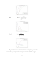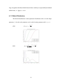
1
Prices of Credit Default Swaps and the Term Structure of Credit Risk
by
_______________________________________
Mary Elizabeth Desrosiers
A Professional Master’s Project
Submitted to the Faculty
of the
WORCESTER POLYTECHNIC INSTITUTE
in partial fulfillment of the requirements for the
Degree of Master of Science
in
Financial Mathematics
May 2007
APPROVED:
________________________________________
Professor Domokos Vermes, Advisor
Executive Summary
Investments in any form of financial product, other than a bank deposit at the riskfree interest rate, involve some sort of risk due to the volatility of the economy. Interest
rate risk is the most critical risk factor affecting fixed income securities. However, the
growing credit derivatives market is based primarily on credit or default risk. This is the
risk caused by the possibility that a company will have financial troubles and will have to
default on payments which it owes to its lenders. US treasury securities are considered to
be free of credit risk because they are backed by the government. In order to protect
investors from this risk, the credit derivatives market emerged with various products
whose sole purpose is to hedge credit risk. A credit derivative is a contract between a
protection buyer and a protection seller to transfer the credit risk of an asset without the
actual transfer of the asset.
The most fundamental credit derivative is the credit default swap. In a credit
default swap, the protection buyer makes periodic premium payments to the protection
seller in exchange for the promise that if default occurs, the protection seller will receive
the defaulted security and repay the protection buyer a percentage of what was owed. The
premiums of the credit default swap contract are determined by the market’s view of how
likely it is that default will occur before the credit swap matures. Time-to-default is a
random variable which characterizes the term-structure of credit risk and affects the price
of credit derivative products.
This project quantifies the connection between the prices of the credit default
swaps and the probability distribution of the time-to-default in both directions.
2
1. We calculate the market perceived probabilities and timing of possible default by
a particular borrower from the market prices of a series of traded credit default
swaps referencing the same borrower’s debt.
2. We calculate the fair prices of the credit default swaps from the probability
distribution of the default time and of the recovery rate.
The calculations are implemented in spreadsheets of a Microsoft Excel workbook.
The results of the project can also be used to determine prices of more complex
credit derivates. The market-implied default probabilities determine the credit risk
inherent in all securities depending on the same borrower. They can then be used as input
into more complicated models for multi-name credit derivative products, such as basket
default swaps and collateralized debt obligations.
3
Abstract
The objective of this project is to investigate and model the quantitative connection
between market prices of credit default swaps and the market perceived probability and
timing of default by the underlying borrower. We quantify the credit risk of a borrower in
a two-way relationship: calculate the term structure of default probabilities from the
market prices of traded CDSs and calculate prices of CDSs from the probability
distribution of the time-to-default.
4
Table of Contents
Executive Summary ............................................................................................................ 2
Abstract ............................................................................................................................... 4
Table of Contents................................................................................................................ 5
1. Introduction..................................................................................................................... 6
2. Tradable Assets and Risk Factors ................................................................................... 6
2.1 Fixed Income Products ............................................................................................. 6
2.1.1 Bonds ................................................................................................................. 7
2.1.2 Swaps ................................................................................................................. 7
2.1.3 Asset-backed Securities ..................................................................................... 8
2.2 Risk Factors .............................................................................................................. 9
2.2.1 Interest Rate Risk............................................................................................... 9
2.2.2 Default/Credit Risk .......................................................................................... 10
3. Credit Derivatives ......................................................................................................... 12
3.1 Credit Derivative Products...................................................................................... 13
4. Probability of Default ................................................................................................... 14
4.1 Typical default time distributions ........................................................................... 16
4.1.1 Exponential Distribution.................................................................................. 16
4.1.2 Gamma Distribution......................................................................................... 17
4.1.3 Weibull Distribution ........................................................................................ 19
4.2 Approximation of Default Time Distributions ....................................................... 20
4.2.1 Piecewise Constant CDF.................................................................................. 21
4.2.2 Piecewise Constant Density Function.............................................................. 21
4.2.3 Piecewise Constant Hazard Rate Function ...................................................... 21
5. Credit Default Swaps (CDS)......................................................................................... 21
5.1 CDS Pricing ............................................................................................................ 23
6. CDS Spreadsheet .......................................................................................................... 25
6.1 Computing the Hazard Rates .................................................................................. 26
6.2 Computing the Prices.............................................................................................. 26
7. Conclusions................................................................................................................... 27
Appendix: Workbook User Manual.................................................................................. 28
Bibliography ..................................................................................................................... 32
5
1. Introduction
Credit risk is becoming an increasingly important topic for evaluation in the
financial industry. Up until the recent growth of the credit derivatives market, interest
rate risk was one of the only risk factors taken into consideration when evaluating fixedincome securities. Interest rate risk still remains the most important risk factor to consider
because it affects the entire market, but credit risk is important when it comes to debt
instruments based strictly on credit. There are many different types of credit derivative
products, all falling into two categories: single-name credit derivatives and multi-name
credit derivatives. Single-name credit derivatives are based on the default risk of one
particular company, while multi-name credit derivatives reference the correlation
between the credit risks of various companies. The most fundamental single-name credit
derivative and the basis for many more intricate credit products is the credit default swap.
A credit default swap provides insurance to the buyer against a credit event such as
default. Probability of default plays an important role in pricing credit default swaps, but
this probability is not always known. This paper introduces methods to derive the market
perceived probability of default which can then be used to price credit default swaps or
other credit derivative products.
2. Tradable Assets and Risk Factors
2.1 Fixed Income Products
A common form of investment is a fixed income security. Fixed income securities
come in many forms and differ from other variable-income securities, such as stocks, in
that all payments are known in advance. A fixed income investor lends its money in
exchange for a promise of a pre-determined sequence of payments by the counterparty,
6
also known as the debt issuer. Fixed-income securities are also known as debt or credit
instruments; the investor credits its money to the issuer, who assumes the debt. Fixed
income products are structured based on the “time value of money”: a dollar received
today is different from a dollar to be received one year from today (Risk Glossary, 2007).
2.1.1 Bonds
A bond is a form of securitized debt which matures at a specified date in the
future, pays interest periodically in the form of coupon payments, and repays its facevalue at maturity. A zero-coupon is a special kind of bond which provides only one
payment at the bond’s maturity date consisting of the accrued interest and the principal
portion of the bond. Bonds can be traded. At any point in time, the fair price of a bond is
the present value of its future cash flows.
The price of a bond can fluctuate due to many factors; the most important being
interest-rate sensitivity. As market interest rates change, the present value of future cash
flows changes, affecting the market price of the bond. Another key factor in bond price
movements is the perceived credit quality of the bond issuer. Future payments are only
certain once received, so if the market senses an increased probability that the issuer will
default on some or all of the future payments, the value of the bond depreciates.
Quantifying this credit sensitivity of fixed-income securities is the main focus of this
project.
2.1.2 Swaps
A swap is an over-the-counter (OTC) financial derivative in which two parties
enter into an agreement to exchange a series of cash flows based on the value of an
underlying asset, but that underlying asset is not directly traded. The cash flows can be
7
determined in any manner suitable to both parties’ objectives, as long as the present
values of both cash flows are equal. Swaps have many uses such as hedging, speculation,
and asset-liability management, and they are classified by the nature of the cash flow
streams being exchanged. The most important types are interest-rate swaps, foreign
exchange swaps, and credit related swaps. An interest rate swap is useful for exchanging
fixed rate future cash flows against variable rate future cash flows. Foreign exchange
swaps are agreements to exchange future cash flows of different currencies. Credit
related swaps are the main topic of this project and will be explained in further detail
below.
2.1.3 Asset-backed Securities
An asset-backed security is a fixed-income product based on a specified pool of
underlying assets. The assets, or collateral, are pooled together to form a single portfolio
product that offers lower investment risk through diversification. Typical asset-backed
securities are different combinations of highly illiquid assets such as bonds, loans,
mortgages, and credit instruments. A common asset-backed security is a collateralized
debt obligation (CDO). A CDO is a broad term that encompasses various securities based
on the specific type of debt by which they are backed. Some examples of specific CDOs
are: Collateralized Bond Obligations (CBOs), Collateralized Loan Obligations (CLOs),
Collateralized Mortgage Obligations (CMOs), etc. CDO investors assume the credit risk
of the pooled assets without assuming the credit risk of an individual provider (Risk
Glossary, 2007).
8
2.2 Risk Factors
Risk requires uncertainty and exposure to that uncertainty. The level of
uncertainty and exposure determines the level of risk (Risk Glossary, 2007). Investments
in any form of financial product, other than a bank deposit at the risk-free interest rate,
involve some sort of risk due to the volatility of the economy. Risk comes in many forms
and is a major factor involved in pricing financial products and in investor decisionmaking. Normally the more risk involved, the better the return on the investment and vice
versa. Risks on investments can be grouped into two categories: systematic and
unsystematic. Systematic risks are risks which affect the entire market, or a whole market
sector. Unsystematic risk has an affect on a smaller, specific group of investments, or
even one individual security. While unsystematic risk can be reduced through methods
such as diversification, hedging, and leveraging, systematic risk can only be reduced by
hedging (“Risk”, 2007).
2.2.1 Interest Rate Risk
Interest rates are a form of systematic or market risk because any change affects
the entire market. Interest rates are constantly changing due to the economy and market
fluctuations. Fixed and floating interest rates pose risks on investors. An investment in a
floating rate asset will depreciate if interest rates drop over time. Risks also arise with
fixed rate assets if maturities on assets and liabilities in a portfolio are mismatched. Once
an asset or a liability matures, if interest rates have changed, this has an affect on the
overall portfolio value.
Interest rate risk is the most critical risk factor affecting fixed income securities. It
is the primary cause for market price fluctuations. The varying level of exposure to
interest rate risk is the cause for the difference between the interest rate spreads on short
9
and long term bonds. The interest rate spread is the difference between the interest rate
available on a US treasury security of a given maturity and the risk-free interest rate. The
interest rate spread graphed as a function of maturity time is known as the term-structure
of interest rates.
Interest rate risk inherent in a fixed income security can be reduced, increased, or
even eliminated through hedging; taking an offsetting position in a related security.
Commonly used hedging instruments are interest rate swaps, interest rate options, caps,
floors, swaptions, and other interest rate derivatives.
2.2.2 Default/Credit Risk
Credit risk is the second most critical risk factor affecting debt instruments. This
is the risk caused by the possibility that the issuer of the bond may not be able to meet its
obligations to pay interest or repay the principal of the loan. US treasury securities are
considered to be free of credit risk. The difference between the interest rate offered on a
bond of a particular issuer and the interest rate on the US treasury bond of the same
maturity is called the credit spread. The credit spread depends on the credit quality of the
issuer and on the maturity of the bond. The credit spread is the reward an investor
receives for assuming the credit risk inherent in the security.
Default risk is an important factor to take into consideration when making an
investment in a fixed income product, such as a bond. Default occurs when the bond
issuer is unable to settle the remaining debt on a bond. This leads to the investor losing
the remainder of their future coupon payments and the principal portion of the bond.
Depending on the terms set forth in the initial agreement, the investor may be able to
recover a percentage of their investment based the specific recovery rate involved. The
10
recovery rate of a bond is “the fraction of the outstanding obligation expected to be
recovered through bankruptcy proceedings or some other form of settlement” (Risk
Glossary 2007). Default risk can be assessed prior to purchasing a bond by investigating
the credit ratings of the bond issuer. Standard & Poor’s and Moody’s Investors Service
are two of the largest credit rating agencies which give companies credit ratings based on
those companies’ abilities to pay back their outstanding debt. These ratings reflect a
company’s risk of default on their obligations, ultimately reflecting the company’s
overall credit risk.
Figure: Bond Rating Codes (“Bond Ratings”, 2005)
Rating
S&P Moody's
Highest quality
AAA Aaa
High quality
AA
Aa
Upper medium quality
A
A
Medium grade
BBB Baa
Somewhat speculative
BB
Ba
Low grade, speculative
B
B
Low grade, default
possible
CCC Caa
Low grade, partial
recovery possible
CC
Ca
Default, recovery unlikely
C
C
The credit ratings are based on the company’s probability of default, their average
recovery rates on previous defaults, and the quality and diversification of their assets. The
higher the risk of default or the lower the credit rating of a company, the higher the yield
the investor should receive on the bond. Yield is the annual rate of return of an investment.
The highest quality bonds, for example AAA, offer minimal credit risk and the lowest
11
yield. As the quality decreases, credit risk increases, but lower quality bonds have much
higher yields. Higher risk should give higher returns.
Credit risk inherent in a debt instrument, and consequently the credit spread,
depends on the following factors:
1. The probability of a default by the issuer.
2. The timing of a possible future default
3. The probability distribution of the recovery rate.
Assuming a constant and known recovery rate, the term-structure of the credit spread (i.e.
the credit risk) has a one-to-one correspondence with the probability distribution of the
time of default for the given issuer.
One of the main goals of this project is to use market prices of traded credit
derivatives to recover the market’s perception of the probability distribution of the time
of default for the issuer.
3. Credit Derivatives
Upon purchasing a fixed income product, the investor faces the risk of financial
loss if the issuer defaults on the obligation. In order to protect themselves or to hedge this
risk, investors have the option of buying a credit derivative. A credit derivative is a
contract between a protection buyer (for example, the owner of a bond) and a protection
seller (a third party financial institution) to transfer the credit risk of an asset without the
actual transfer of the asset. The idea is to avoid direct ownership of the asset in the
transaction in order to minimize losses in the event of default.
12
3.1 Credit Derivative Products
There are many different types of credit derivative products, each based on the
specific risk being transferred. The two fundamental categories of credit derivatives are
single-name credit derivatives and multi-name credit derivatives.
•
Single-name credit derivatives offer protection against the default risk of one
particular borrower. Examples are asset swaps, credit linked notes, and credit
default swaps.
•
Multi-name credit derivatives are based on defaults of one or more borrowers
from a group of borrowers. These instruments depend not only on the credit risks
posed by the individual borrowers, but also on the correlation between them.
Examples of multi-name credit derivatives are basket default swaps and CDOs.
A total return swap (TRS), also known as a total rate of return swap (TRORS), is
a credit derivative intended to protect against depreciation of an asset. The swap
exchange is a combination of an underlying asset and an interest rate swap. In the TRS
agreement, one party receives the total return, or the generated income from the asset plus
any capital gains, while the other party receives payments based on a set rate as part of
the interest rate swap. The owner of the asset gets protection against any loss in value,
while the counterparty receives the benefits of the asset without having to put the asset on
its balance sheet (Investopedia, 2007). An asset swap is quite similar to a total return
swap in that it consists of a bond paired with an interest rate swap. An investor purchases
a bond and then hedges out the interest rate risk with an interest rate swap. The major
difference between an asset swap and a total return swap is that in the event of default,
13
the total return swap terminates while the interest rate swap payments of the asset swap
continue until maturity.
A credit-linked note (CLN), or credit default note, is a product issued by a Special
Purpose Vehicle (SPV) offering investors periodic payments plus the par value of the
reference entity at maturity, unless default occurs. The SPV also enters into a credit
default swap with a third party which pays the SPV an annual fee. This annual fee
provides higher return to investors to compensate for the credit risk involved. In the event
of default, the investors receive a portion of the par value based on the recovery rate, and
the SPV pays the third party the par value minus the recovery rate.
A collateralized debt obligation (CDO) is also a form of credit derivative. In a
cash flow CDO, the investor faces credit risk based on the pool of underlying bonds or
loans. A CDO is a pool of assets packaged into one portfolio, and then that portfolio is
tranched. It is split up into sections, each corresponding to a different level of loss. The
tranches provide the investor with some flexibility in choosing the amount of loss or
credit risk to which they are willing to be exposed. In a synthetic CDO, a CDO made up
of credit default swaps, the investor faces credit risk based on the credit worthiness of the
underlying companies.
There are many variations of these products, but the most common and important
credit derivative is the credit default swap (CDS) which will be explored in detail in
Chapter 5.
4. Probability of Default
The premiums of the credit default swap contract are determined by the market’s
view of how likely it is that default will occur before the reference entity matures. The
14
probability distribution of the time-to-default is the term-structure of credit risk and is
one of the driving factors behind the credit derivatives market. Default is an event which
is modeled using probability theory and statistics. Time-to-default is a random variable, τ
with non-negative values, which can be characterized by its cumulative probability
distribution function F, its probability density function f, or hazard rate function h.
Common probability distributions that are used to model the probability of default are the
exponential, gamma, and Weibull distributions.
The cumulative distribution function (cdf) F(t) gives the probability that the
default occurs before time t.
F (t ) = P (τ < t )
The probability density function (pdf) f(t) is the derivative of the cumulative distribution
function, whenever F is differentiable.
f (t ) =
d
F (t )
dt
or
t
F (t ) =
∫ f (s)ds
−∞
The probability that default will occur in a small time interval of length Δt around time t
can be approximated as f(t)·Δt.
f (t ) ⋅ Δ t ≈ P (t < τ < t + Δ t )
The hazard rate h(t) is the conditional density function of the default time τ, conditioned
on the event that no default has occurred before time t.
h(t ) = lim P(t < τ < t + Δt | τ > t ) =
Δt → 0
15
f (t )
1 − F (t )
The probability density function can be recovered from the hazard rate function by the
following formula:
− t h( s ) ds
f (t ) = h(t ) ⋅ e ∫0
4.1 Typical default time distributions
4.1.1 Exponential Distribution
CDF:
F (t ) = 1 − e −λ ⋅t if t > 0
PDF:
f (t ) = λ ⋅ e − λ ⋅t if t > 0
16
Hazard:
h(t ) = λ
The exponential distribution is characterized by a unique “memoryless” property.
In relation to probability of default, “memoryless” indicates that at any given time, the
probability of default is distinct and does not depend on information from the past.
Memorylessness is a form of conditional probability, that for any positive real numbers s
and t, we have
P (T > t + s | T > t ) = P (T > s )
This memorylessness property implies that the hazard rate is constant.
4.1.2 Gamma Distribution
The gamma distribution is the sum of k>0 independent, exponentially distributed
random variables. The gamma distribution has two parameters, k and β, where k is the
shape parameter and β is the scale parameter. A special case of the gamma distribution is
when k=1, we have the exponential distribution with λ=1/β.
t
CDF:
F (t ) =
∫x
k −1 − x / β
dx
∫x
k −1 − x / β
dx
0
∞
e
e
0
17
PDF:
e −t / β
f (t ) = t k −1
∞
β k ∫ x k −1e − x / β dx
0
Hazard:
h(t ) =
t k −1e − t
∞
∫x
k −1 − x / β
e
dx
t
The gamma distribution is suitable for default time modeling if it is perceived that
a borrower has to go through a number of stages of crisis before it defaults. As t gets
18
large, the gamma distributed default times behave similarly to exponentially distributed
default times, i.e. lim h(t ) = const .
t →∞
4.1.3 Weibull Distribution
The Weibull distribution is a three parameter distribution with α>0 as the shape
parameter, λ>0 as the scale parameter, and γ as the location parameter with -∞<γ<∞.
α
⎛ t −γ ⎞
−⎜
⎟
⎝ λ ⎠
CDF:
F (t ) = 1 − e
PDF:
α ⎛t −γ ⎞
f (t ) = ⎜
⎟
λ⎝ λ ⎠
19
α
α −1
e
⎛ t −γ ⎞
−⎜
⎟
⎝ λ ⎠
Hazard:
h(t ) =
α ⎛t −γ ⎞
⎜
⎟
λ⎝ λ ⎠
α −1
The Weibull distribution is a form of extreme value distribution. An extreme
value distribution is a limiting distribution for the minimum and maximum of a large
collection of random observations from the same distribution. In terms of probability of
default, the Weibull distribution governs the time until default of the first to default from
a collection of default times.
4.2 Approximation of Default Time Distributions
In real life, not enough information is available about the time-of-default to
determine its probability distribution at every time t. Usually, it is possible to estimate the
probability that the default will happen in various time intervals of positive length (e.g. 6
months, 1 year, etc.). In such cases, the probability distribution of the continuous random
variable τ must be determined by some interpolation procedure.
The main assumption behind these techniques is that default occurs at particular
discrete times. This assumption is supported by the fact that borrowers usually declare
bankruptcy when they are unable to meet an interest payment, so defaults often occur on
coupon payment dates. Probabilistically this means that the time-to-default is a step
function.
20
4.2.1 Piecewise Constant CDF
A piecewise constant CDF jumps from one step to the next at the discrete times
when default is possible (e.g. the semi-annual coupon dates). The size of each jump
corresponds to the probability of default at that particular time. Piecewise constant CDFs
are not differentiable, hence density and hazard functions are not defined in such cases.
4.2.2 Piecewise Constant Density Function
This approximation assumes that between discrete jump points of the probability
density function the default time is uniformly distributed. In other words, within those
intervals of constancy, default is equally probable at any time. Piecewise constant density
functions imply piecewise linearly interpolated CDF. The corresponding hazard rate
graph consists of adjoining hyperbolic curves.
4.2.3 Piecewise Constant Hazard Rate Function
A piecewise constant hazard rate assumes that between discrete jump points of the
step function, the default time follows the exponential distribution with constant hazard
rate. Piecewise constant hazard rate is the assumption used in this project and the method
used in the spreadsheet for modeling time-to-default.
5. Credit Default Swaps (CDS)
A credit default swap is a contract, indexed to a single reference asset, which
provides insurance against a default event on that asset. There are three parties involved
in a credit default swap. The first is the protection buyer; this is the investor and owner of
the reference asset, for example a General Motors bond. The bond issuer, General Motors
in this example, is the second party that plays a role, indirectly, in the CDS. Based on the
bond investment, General Motors pays the investor periodic coupon payments and
21
promises to pay the principal portion of the bond at a set maturity date. After purchasing
the bond, the investor becomes nervous that General Motors will suffer a credit event and
default on its promised, future payments. So, the bond owner purchases protection
against the possibility of this credit event in the form of a credit default swap. The CDS is
a contract between the protection buyer and a protection seller. The latter is typically an
insurance company or a securities company, e.g. Morgan Stanley. In this agreement, the
protection buyer makes periodic premium payments (periods are usually half year
increments) to the protection seller, in this case Morgan Stanley, and Morgan Stanley
agrees to pay the entire face value of the bond to the protection buyer if General Motors
defaults on the bond. The CDS will terminate either at the bond’s maturity or the date a
default event occurs, whichever comes first. If default never occurs, General Motors
continues to pay the periodic coupon payments and at maturity pays the principal portion
of the bond to the investor, and the investor pays the CDS premium payments to Morgan
Stanley until the bond matures. Morgan Stanley will never have to make any payments
and profits for assuming the credit risk of the bond. If a default event occurs before the
set maturity, Morgan Stanley instantly compensates the protection buyer for its loss and
has no further obligations in the CDS contract. In this event, the investor would have
minimized its losses by entering into the credit default swap.
The credit default swap is the basis for the credit derivatives market. In 2001,
credit default swaps accounted for 38% of the credit derivatives market, which was more
than two times that of the next highest contributor. Today, credit default swaps continue
to dominate the market, and are used as the foundation of newer, more complicated
22
products. For example, a credit default swap index (CDSI) is a single product based on a
basket of credit entities (Investopedia, 2007).
Figure 1: Market Share of Outstanding Notional for Credit Derivative Products (Credit Derivatives
Explained, 2001)
Credit Derivative Instrument Type
Market Share
(% Notional) at End 1999
Credit Default Products
38%
Portfolio/CLOs
18%
Asset Swaps
12%
Total Return swaps
11%
Credit Linked Notes
10%
Baskets
6%
Credit Spread products
5%
An investor in a CDS only assumes the credit risk of default on the reference
entity; all other risks such as interest rate movements do not have an affect on the CDS
agreement.
5.1 CDS Pricing
The main idea behind pricing models for credit default swaps is that they are
completely independent from interest rate movements. The only risk assumed is that of
default, or credit risk. The price of the CDS is determined by setting the present value of
the periodic premium payments equal to the present value of the reference entity at
maturity, or time of default. It is common to think of a CDS as having two opposing legs:
the premium leg corresponding to the fixed premiums payments and the default leg
corresponding to the contingent payment upon default (Arvanitis, 2001).
The premium leg is a stream of discounted, fixed cashflows at fixed times (t0, t1,
t2…, tn). These annualized premium payments, X, are paid until maturity, T = tn, or
23
default, τ, whichever occurs first. This stream of cashflows is discounted back by the
risk-free discount factor, В(0,ti), and weighted by the instantaneous probability of default
h(t), or hazard rate, to achieve the present value.
Equation 1: Present Value of Premium Leg
PV ( PL) = K ⋅ ∑ (t i − t i −1 ) ⋅ X ⋅ B (0, t i ) ⋅ P (τ > t i )
where
ti
P (τ > t i ) = exp(− ∫ h(u )du )
0
The default leg (DL) is the payment contingent upon default, (1-δ) where δ is the
assumed recovery rate, discounted back using the risk-free discount factor and the
conditional probability of default at time ti.
Equation 2: Present Value of Default Leg
PV ( DL) = K ⋅ (1 − δ ) ⋅ ∑ B(0, t i ) ⋅ P(t i −1 < τ < t i )
(K represents the notional amount and δ is the recovery rate.)
Equation 3: Present Value of Swap
PV Swap = PV ( DL) − PV ( PL)
so
i
PV Swap = K ⋅ ∑ B(0, t k ) ⋅ P (τ > t k −1 ) ⋅ [(1 − δ )(1 − α k ) − (t i − t i −1 ) ⋅ X ⋅ α k ]
k =1
where
h(t i ) = α i
When a swap is initiated, the premium payments are determined by setting the
present value of the premium leg and default leg equal to zero; in doing so, neither party
pays anything at the start of the swap contract.
K ⋅ ∑ (t i − t i −1 ) ⋅ X ⋅ B (0, t i ) ⋅ P (τ > t i ) = 0
K ⋅ (1 − δ ) ⋅ ∑ B (0, t i ) ⋅ P (t i −1 < τ < t i ) = 0
24
Equation 4: Initial Present Value of CDS
i
PV Swap = 0 = K ⋅ ∑ B (0, t k ) ⋅ P (τ > t k −1 ) ⋅ [(1 − δ )(1 − α k ) − (t i − t i −1 ) ⋅ X ⋅ α k ]
k =1
with
i −1
P (τ > t k −1 ) = ∏ α k
k =1
We now have an equation that we can use to solve for either the premium
payments, XT, or the hazard rates, αi, depending on what data is known.
6. CDS Spreadsheet
The main goal of this project is to use credit default swaps to determine the
market’s perception of the risk-neutral probability of default, using a predetermined
constant recovery rate. The workbook constructed for this serves two major purposes:
1. Derive the implied market hazard rates using market quotes for credit default
swap premiums.
2. Price credit default swaps of different maturities using derived market hazard
rates.
The workbook draws from market quoted premiums of credit default swaps of
different maturities on the same reference credit to determine the implied hazard rate
which models the default probability distribution. The spreadsheet user can then use the
market’s perceived default probability distribution as a parameter to get the risk-neutral
price of credit default swaps. Both spreadsheet applications require the use of Equation 4
and solving a set of non-linear equations using the Solver Add-In in Microsoft Excel.
(See Appendix: Worksheet User Manual for instructions on how to operate the
spreadsheet.)
25
6.1 Computing the Hazard Rates
“Bootstrapping” is a calibration procedure used by the workbook to solve for the
hazard rates. We began by gathering market premiums for current default swaps with
different maturities on the same reference entity. Then we assume the hazard rates, αi for
time intervals [ti-1,ti], are piecewise constant between the maturity dates of the individual
market swaps. We extract the hazard rates by solving for the appropriate αi using
Equation 4 and a constant recovery rate, δ. We solve for each αi in order of increasing
maturity, using the data from the swap with the first maturity T1 to solve for α1.
Consequently we know α1 and have the data from T2 to solve for α2 and so on. This
probability stripping procedure gives us a step-function for the hazard rates
corresponding to the credit default swaps.
These piecewise constant hazard rates form a step function with jumps at the
different maturity dates. The workbook shows this step-function and then takes this stepfunction and smoothes it using cubic splines. This smoothed curve represents a
continuous hazard of default.
6.2 Computing the Prices
Assuming a constant recovery rate and using given or derived hazard rates, the
workbook prices credit default swaps of various maturities. Similarly to the above hazard
rate procedure, the workbook uses Equation 4 and the corresponding hazard rates to
compute the premiums.
26
7. Conclusions
The price of a credit default swap and the probability of default are directly
connected. Quantifying the default probability and term structure is useful for hedging
out credit risk inherent in fixed-income securities and is also helpful for calculating the
risk-neutral prices of credit derivatives other than CDSs.
These market perceived hazard rates which this pricing model computed can be
integrated into more complicated models for multi-name credit derivative products, such
as basket default swaps or CDOs. Other extensions of this project could be to incorporate
stochastic recovery rates or stochastic hazard rates.
27
Appendix: Workbook User Manual
The first step in using the workbook is to gather market prices for credit default swaps on
the reference entity for which you want to determine the probability of default for as
many different maturities that are available. Also, determine the following parameters
that will be used: size of time intervals between maturity dates, the term structure of the
risk-free interest rate, your reference entity’s notional amount, and the assumed constant
recovery rate.
The workbook contains macros, so before opening the workbook it is necessary to set the
macro security to an appropriate level which allows for running these macros.
Upon opening the file, the first page you should see is the “Input” sheet. If this does not
open up directly, click on the “Input” tab.
“Input” tab
28
Input the following parameters into the appropriate blue cells in column H: size of time
intervals between maturity dates, risk-free interest rate, your reference entity’s notional
amount, and the constant recovery rate.
Input the market premiums you previously gathered in the blue cells of Option 1 for the
appropriate corresponding maturity dates.
To compute the hazard rates, go to the “Hazard Rates” tab. Open Solver by going to the
Tools drop down menu, and selecting Solver. If Solver is not previously installed into
your version of Excel, you must first install it by clicking on the Tools drop down menu,
then select Add-Ins. Check the box next to the Solver Add-In and click OK. Click on Yes
when prompted with the option to install solver now. Solver should now be listed in the
Tools drop down menu. Once you open solver, you will be prompted to enter the Solver
Parameters.
29
You are going to want to solve for the appropriate present value equation in row #8,
beginning with C8 and going in order to the right, until you end on cell L8. In the Solver
Parameters menu, you want to “Set target cell:” first to cell C8. “Equal to:” the “Value
of:” 0. And in the box where it says “By changing cells” you want to select the cell of
what you are solving for. For α1, this is cell C19. Then click the solve button. The
corresponding hazard rate for the CDS with maturity 0.5 years should appear in the
purple cell C19. You want to repeat this process using Solver 10 times to solve for the
hazard rates in row #19, starting at C19 and moving to the right one cell at a time until
you solve for the final hazard rate, cell L19.
30
The computed hazard rates and resulting hazard rate step function can be found by
clicking the Hazard Rate Step Function tab. A smoothed hazard rate function can be
viewed on the “Smooth Hazard Rate Function” tab. And the corresponding probability
distribution can be viewed on the “Probability Distribution” tab.
To compute the Premiums of the CDS, input the hazard rates into the blue cells of Option
2 next to the appropriate maturity dates. Then go to the “Premiums” tab, and you will
need to use Solver in the same manner as described above to compute the hazard rates.
The only difference is that you will be solving for the cells in row #13. So for the
premium payment for the first CDS with maturity 0.5 years, you will use Solver and Set
target cell C8 “Equal to:” the “Value of:” 0, “By changing cells:” C13. Repeat this 10
times in increasing order until you solve for cell L13. The resulting premiums will be
shown in the purple cells in row #13.
Any time you change any data, you need to run the Solver over again for every cell you
wish to solve for.
31
Bibliography
Arvanitis, Angelo and Jon Gregory. Credit: The Complete Guide to Pricing, Hedging and
Risk Management. Risk Waters Group Ltd: London, 2001.
"Bond Basics." Investopedia. 2007. Investopedia Inc. Feb.-Mar. 2007
<http://www.investopedia.com/university/bonds/default.asp>
"Bond Ratings." Fidelity Investments. 2005. FMR Corp. Jan.-Feb. 2007
<http://personal.fidelity.com/products/fixedincome/bondratings.shtml>
Bowers, Gerber, Hickman, Jones, and Nesbitt, ed. Actuarial Mathematics. Illinois: The
Society of Actuaries, 1997. 2nd edition.
Credit Derivatives Explained: Market, Products, and Regulations. Lehman Brothers
International (Europe). March 2001: 3-42.
Galiani, Stefano S. “Copula Functions and their Application in Pricing and Risk
Managing Multiname Credit Derivative Products.” King’s College London.
September 2003: 27-33.
Gordy, Michael B., ed. Credit Risk Modelling: the Cutting Edge Collection. London:
Risk Books, 2003.
Jackson, Mary and Mike Staunton. Advanced Modelling in Finance using Excel and
VBA. New York: John Wiley & Sons, Ltd.
Li, David X. “On Default Correlation: A Copula Function Approach.” The RiskMetrics
Group. April 2000: 1-11.
"Risk Glossary." 1996-Current. Contingency Analysis. 13 Feb.-Mar. 2007
<http://www.riskglossary.com/>
“Risk.” Investopedia. 2007. Investopedia Inc. Feb.-Mar. 2007
<http://www.investopedia.com/terms/r/risk.asp>
Shimko, David, ed. Credit Risk: Models and Management. London: Risk Books, 1999.
32