1
User Manual for the GROOVE Tool Set
Arend Rensink, Iovka Boneva, Harmen Kastenberg and Tom Staijen
Department of Computer Science, University of Twente
P.O.Box 217, 7500 AE Enschede, The Netherlands
{rensink,bonevai,h.kastenberg,staijen}@cs.utwente.nl
November 12, 2012
Contents
1
2
3
4
5
Introduction
1.1 Toolkit Components .
1.2 Getting it running . .
1.2.1 Download . .
1.2.2 Installation .
.
.
.
.
.
.
.
.
.
.
.
.
.
.
.
.
.
.
.
.
.
.
.
.
.
.
.
.
.
.
.
.
.
.
.
.
.
.
.
.
.
.
.
.
.
.
.
.
.
.
.
.
.
.
.
.
.
.
.
.
.
.
.
.
.
.
.
.
.
.
.
.
.
.
.
.
.
.
.
.
.
.
.
.
.
.
.
.
.
.
.
.
.
.
.
.
.
.
.
.
.
.
.
.
.
.
.
.
.
.
.
.
.
.
.
.
.
.
.
.
.
.
.
.
.
.
.
.
.
.
.
.
.
.
.
.
2
2
2
2
3
Basic Concepts
2.1 Graphs . . . . . . . . . . . . . . . .
2.2 Rules . . . . . . . . . . . . . . . .
2.3 Negations . . . . . . . . . . . . . .
2.4 Equalities, Mergers and Injectivities
2.5 Rule Comments . . . . . . . . . . .
2.6 Rule properties . . . . . . . . . . .
2.7 Transition systems . . . . . . . . .
2.8 Typing . . . . . . . . . . . . . . . .
.
.
.
.
.
.
.
.
.
.
.
.
.
.
.
.
.
.
.
.
.
.
.
.
.
.
.
.
.
.
.
.
.
.
.
.
.
.
.
.
.
.
.
.
.
.
.
.
.
.
.
.
.
.
.
.
.
.
.
.
.
.
.
.
.
.
.
.
.
.
.
.
.
.
.
.
.
.
.
.
.
.
.
.
.
.
.
.
.
.
.
.
.
.
.
.
.
.
.
.
.
.
.
.
.
.
.
.
.
.
.
.
.
.
.
.
.
.
.
.
.
.
.
.
.
.
.
.
.
.
.
.
.
.
.
.
.
.
.
.
.
.
.
.
.
.
.
.
.
.
.
.
.
.
.
.
.
.
.
.
.
.
.
.
.
.
.
.
.
.
.
.
.
.
.
.
.
.
.
.
.
.
.
.
.
.
.
.
.
.
.
.
.
.
.
.
.
.
.
.
.
.
.
.
.
.
.
.
.
.
.
.
.
.
.
.
.
.
.
.
.
.
.
.
.
.
.
.
.
.
.
.
.
.
.
.
.
.
.
.
.
.
.
.
.
.
.
.
.
.
.
.
.
.
.
.
.
.
.
.
.
.
.
.
3
3
4
6
6
8
8
9
9
Advanced Concepts
3.1 Wildcards and Variables
3.2 Regular Expressions . .
3.3 Data Attributes . . . . .
3.4 Rule Parameters . . . . .
3.5 Control . . . . . . . . .
3.6 Nested Rules . . . . . .
3.7 System Properties . . . .
.
.
.
.
.
.
.
.
.
.
.
.
.
.
.
.
.
.
.
.
.
.
.
.
.
.
.
.
.
.
.
.
.
.
.
.
.
.
.
.
.
.
.
.
.
.
.
.
.
.
.
.
.
.
.
.
.
.
.
.
.
.
.
.
.
.
.
.
.
.
.
.
.
.
.
.
.
.
.
.
.
.
.
.
.
.
.
.
.
.
.
.
.
.
.
.
.
.
.
.
.
.
.
.
.
.
.
.
.
.
.
.
.
.
.
.
.
.
.
.
.
.
.
.
.
.
.
.
.
.
.
.
.
.
.
.
.
.
.
.
.
.
.
.
.
.
.
.
.
.
.
.
.
.
.
.
.
.
.
.
.
.
.
.
.
.
.
.
.
.
.
.
.
.
.
.
.
.
.
.
.
.
.
.
.
.
.
.
.
.
.
.
.
.
.
.
.
.
.
.
.
.
.
.
.
.
.
.
.
.
.
.
.
.
.
.
.
.
.
.
.
.
.
.
.
.
.
.
.
.
.
.
.
.
.
.
.
.
.
.
.
.
.
.
.
.
.
.
.
.
.
.
.
.
.
.
.
.
.
.
.
.
.
.
.
.
.
.
.
.
.
.
.
.
.
.
.
.
.
.
.
.
.
.
.
.
.
10
10
11
12
14
16
17
19
Exploration and Model Checking
4.1 Exploration . . . . . . . . . .
4.2 Syntax of Temporal Logic . .
4.3 CTL Model Checking . . . . .
4.4 LTL Model Checking . . . . .
.
.
.
.
.
.
.
.
.
.
.
.
.
.
.
.
.
.
.
.
.
.
.
.
.
.
.
.
.
.
.
.
.
.
.
.
.
.
.
.
.
.
.
.
.
.
.
.
.
.
.
.
.
.
.
.
.
.
.
.
.
.
.
.
.
.
.
.
.
.
.
.
.
.
.
.
.
.
.
.
.
.
.
.
.
.
.
.
.
.
.
.
.
.
.
.
.
.
.
.
.
.
.
.
.
.
.
.
.
.
.
.
.
.
.
.
.
.
.
.
.
.
.
.
.
.
.
.
.
.
.
.
.
.
.
.
.
.
.
.
.
.
.
.
21
21
21
21
21
I/O
5.1 Graphs and rules . . . . . . . . . . . . . . . . . . . . . . . . . . . . . . . . . . . . . . . . . . .
5.2 Control programs . . . . . . . . . . . . . . . . . . . . . . . . . . . . . . . . . . . . . . . . . . .
5.3 System properties . . . . . . . . . . . . . . . . . . . . . . . . . . . . . . . . . . . . . . . . . . .
21
22
23
23
.
.
.
.
.
.
.
.
.
.
.
.
.
.
1
1
Introduction
GROOVE is a project centered around the use of simple graphs for modelling the design-time, compile-time, and
run-time structure of object-oriented systems, and graph transformations as a basis for model transformation and
operational semantics. This entails a formal foundation for model transformation and dynamic semantics, and
the ability to verify model transformation and dynamic semantics through an (automatic) analysis of the resulting
graph transformation systems, for instance using model checking.
This manual constsis of some download and installation instructions and a manual for using the tools included
in the GROOVE tool set. The latter also explains the format used for graphs and graph transformations. Together
with some examples, this should allow you to get started with GROOVE.
1.1
Toolkit Components
The GROOVE tool set includes the following programs:
Simulator: a GUI-based tool that lets you construct, simulate and model check rule systems visually;
Editor: a GUI-based editor that lets you edit individual rules and graphs;
Generator: a command line tool that lets you simulate and model check rule systems without the performance
penalty of the GUI;
Imager: a command line or GUI tool that suppots various conversions from GROOVE graphs and rules to other
visual formats.
1.2
Getting it running
Since the entire GROOVE tool is written in Java, getting it running is extremely easy.
1.2.1
Download
The GROOVE tool is distributed under the Apache License, Version 2.0. A copy of this license is available on
http://www.apache.org/licenses/LICENSE-2.0. The latest GROOVE build can be downloaded from
the GROOVE sourceforge page:
http://sourceforge.net/projects/groove
There are some different distributions of the GROOVE tool set available on the sourceforge site. The groovebin+lib package includes all the libraries below. The groove-bin package is identical but without the libraries. The
groove-src package only includes the sources of the groove project. There are also some examples available in the
groove-samples package. The groove-doc package consists of some publications about GROOVE and the theory
behind it.
The GROOVE library depends on some other libraries, namely:
• A NTLR, for compiling control programs.
See http://www.antlr.org (Version included: 3.4)
• A SM, for Java bytecode manipulation and analysis (in conjunction with G ROOVY, see below).
See http://asm.ow2.org/ (Version included: 4.0)
• G NU P ROLOG, an implementation of ISO Prolog as a Java library.
See http://www.gnu.org/software/gnuprologjava/ (Version included: 0.2.6)
• JG RAPH for displaying graphs and rules.
See http://www.jgraph.com (Version included: 5.13.0)
• EMF for converting to and from Eclipse ECORE format.
See http://eclipse.org (version included: 2.5.0)
• EPSG RAPHICS for exporting displayed graps to EPS format.
See http://www.abeel.be/epsgraphics/ (Version included: 1.2)
• G ROOVY for easy and flexible access to the GROOVE API.
See http://groovy.codehaus.org/ (version included: 2.0.5)
2
• I T EXT for exporting displayed graphs to PDF format.
See http://itextpdf.com/ (Version included: 5.3.2)
• JG OODIES L OOKS for platform-dependent look&feel.
See http://www.jgoodies.com/freeware/libraries/looks/ (Version included: 2.4.1)
• LTL 2 BUCHI, a component to translate LTL formulae to Büchi automata.
See http://ti.arc.nasa.gov/profile/dimitra/projects-tools
• RS YNTAX T EXTA REA, for editing syntax-highlighted control programs.
See http://fifesoft.com/rsyntaxtextarea
1.2.2
Installation
To use the GROOVE tool set, download the bin+lib package from the download site explained above and unzip it
to any location on your computer. Let’s refer to this location as the GROOVE directory.
The bin subdirectory of the GROOVE directory contains jar files for each of the toolkit programs (see Section 1.1), so Simulator.jar, Editor.jar etc. You can use these in either of the following ways:
• In an explorer window opened on the bin directory, double-click the icon of the jar file;
• On the command line, run ‘java -jar GROOVE_PATH\bin\Program.jar [parameters]’, where
GROOVE PATH is the groove directory and Program is the toolkit program in question.
2
Basic Concepts
GROOVE shows rules and graphs using various kinds of graphical embellishments, such as colours, bold and italic
fonts, dashed and dotted outlines, and special symbols. During editing, however, the node and edge labels you
enter do not have those embellishments. Instead, you have to use a fairly rich textual syntax to make the same
distinctions. The prime element in this syntax is a prefix, usually consisting of an identifier followed by a colon
(‘:’).
2.1
Graphs
GROOVE is based on directed node- and edge-labelled graphs. Graph nodes are depicted as boxes, and edges as
arrows between them; the node labels are inscribed in the nodes, the edge labels along or on top of the arrows.
There are two kinds of node labels: types and flags. In the Edit view, these are distinguished from one another
and from edge labels by prefixing them with “type:” and “flag:”, respectively. If you omit the prefix, GROOVE will
interpret the label as an edge label, and it will create a self-edge with that label. (If you have no types or flags in
your graph, self-edge labels remain inscribed in the nodes in the Display view.) In the Display view, types are set
bold and flags are set italic. Here is an example:
Prefix view
type:Library
Display view
has
has
type:Book
flag:reserved
Library
cites
has
Book
reserved
has
cites
(1)
Book
type:Book
cites
cites
Type and flag labels. As seen above, node labels can be either types or flags. There are two important differences:
• Type labels are partially ordered by subtyping (often called inheritance). This affects rule matching: a type
label in a rule matches all subtype labels (i.e., those that are smaller in the partial ordering) of the host graph.
• If a type graph is used, type labels must be unique: every node must have exactly one type label.
3
Prefix
Where?a
rem:
use:
del:
new:
cnew:
not:
bool:
int:
real:
string:
arg:
prod:
let:
test:
par:
parin:
parout:
abs:
sub:
in:
out:
part:
import:
forall:
forallx:
exists:
existsx:
nested:
id:
color:
edge:
path:
:
type:
flag:
NE,HRT
NE,R
NE,R
NE,R
NE,R
NE,R
NE,HRT
NE,HRT
NE,HRT
NE,HRT
E,R
N,R
N,HR
N,R
N,R
N,R
N,R
NE,T
E,T
E,T
E,T
E,T
N,T
N,R
N,R
N,R
N,R
E,R
N,R
N,RT
N,T
E,R
NE,HR
NE,HRT
NE,HRT
Explanation
Remark node or edge; used for documentation purposes
Declares a node or edge to be a reader (the default value)
Declares a node or edge to be an eraser
Declares a node or edge to be a creator
Declares a node or edge to be a conditional creator
Declares a node or edge to be an embargo
On nodes, a boolean value or type; on edges, a boolean operator
On nodes, an integer value or type; on edges, an integer operator
On nodes, a real value or type; on edges, a real operator
On nodes, a string value or type; on edges, a string operator
Argument edge, from a product node to an attribute value
Product node, collecting arguments for an attribute operation
Syntactic sugar for attribute assignment
Attribute condition that must be satisfied for a rule to apply
Anonymous or numbered rule parameter node
Numbered rule input parameter node
Numbered rule output parameter node
Abstract type node or edge
Inheritance edge between node types
Incoming edge multiplicity declaration
Outgoing edge multiplicity declaration
Composite edge declaration
Indicates that the node is imported from another type graph
Universal quantifier node
Non-vacuous universal quantifier node
Existential quantifier node
Optional existential quantifier node
Quantifier nesting edge
User-defined node identity
Defines the text and outline colour of a node or node type
Defines a node type to be a nodified edge
Declares the remainder of the text to be a regular expression label
Declares the remainder of the text to be a literal edge label
Declares the remainder of the text to be a node type
Declares the remainder of the text to be a flag (= node label)
Sampleb
attributed-graphs
attributed-graphs
attributed-graphs
attributed-graphs
attributed-graphs
parameters
inheritance
colours
bridge
a Abbreviations:
b Name
on Node / Edge, resp. in Host graph / Rule / Type graph
of a sample rule system in which this is used, see http://sf.net/projects/groove, samples download
Table 1: Overview of available edit prefixes. (See also the syntax help in the GROOVE Simulator).
Graph label syntax. Node labels and flags are restricted to identifiers; i.e., strings of characters starting with a
letter or underscore, and containing only letters, digits, underscores or dollar signs. It is also recommended, but
not enforced, to use only identifiers for edge labels. If you want to use other labels, start the label (in the Edit
view) with a colon (“:”). The colon will not be part of the actual label: it is an escape character indicating that
what follows should be taken literally. (Thus, an initial colon serves as an “escape” character precisely as an initial
single quote serves as an escape in Excel.) Whitespace other than simple spaces, such as tabs and newlines, cannot
be included in labels.
2.2
Rules
Formally, rules consist of left hand sides, right hand sides and negative application conditions (NACs), all of which
are different graphs, connected by morphisms. In GROOVE these graphs are combined into one single view, and
colour coding is used to distinguish the original components. As a consequence, a GROOVE view of a rule has the
4
following kinds of elements:
Readers. These are nodes and edges that are in both the LHS and the RHS. In both the editor and the display
view, they are depicted just like ordinary graph elements; hence, the outlines are thin and black and the font
colour is black. In the Edit view, the fact that an edge is a reader may be indicated explicitly by including
an (optional) prefix “use:” in front of the label.
Erasers. These are nodes and edges that occur in the LHS but not the RHS, meaning that they must be matched in
order for the rule to apply, but by applying the rule they will be deleted. In the Display view, such elements
are depicted by a thin, dashed blue outline and blue text; moreover, erased node labels (on non-erased nodes)
are prefixed with “lab–”. In the Edit view, erasers are distinguished by a special prefix “del:”. For eraser
nodes, this prefix should appear on its own as a node label; for eraser edges, the prefix is followed by the
edge label.
Creators. These are nodes and edges that occur in the RHS but not the LHS, meaning that they will be created
when the rule is applied. In the Display view, such elements are depicted by a slightly wider, solid green
outline (light grey in a black-and-white representation) and green text; moreover, created node labels (on
non-created nodes) are prefixed with “lab+”. In the Edit view, creators are distinguished by a special prefix
“new:”. For creator nodes, this prefix should appear on its own as a node label; for creator edges, the prefix
is followed by the edge label.
Embargoes. These are nodes and edges that are in a NAC, but not in the LHS. This means that they forbidden:
their presence in the host graph will prevent the rule from being applied. In the Display view, such elements
are depicted by a wide, dashed red outline (darker grey in a black-and-white representation) and red text;
moreover, forbidden node labels (on non-embargo nodes) are prefixed with “!”. In the Edit view, creators
are distinguished by a special prefix “not:”. For embargo nodes, this prefix should appear on its own as a
node label; for embargo edges, the prefix is followed by the edge label.
Conditional creators. These are nodes and edges that occur both in the RHS and in a NAC but not in the LHS.
This means that these elements should not be there before the rule is applied, but will be created by the
rule application. In other words, the effect combines that of creators and embargoes. In the Display view,
conditional creators are depicted by an overlay of the creator and embargo attributes, namely by a spiked
green-and-red outline and green text. In the Edit view, conditional creators are distinguished by a special
prefix “cnew:”. For conditional creator nodes, this prefix should appear on its own as a node label; for
conditional creator edges, the prefix is followed by the edge label.
If a node plays any of the roles of eraser, (conditional) creator or embargo, its incident edges implicitly also have
this role. Thus, in that case the corresponding prefix can be omitted from the edges in the Edit view.
The following rule example contains all of the above types of elements:
Display view
Prefix view
new:a
not:type:B
new:flag:s
del:b
c
d
c
del:
type:C
type:B
not:d
a
d
not:
type:D
!B
+s
new:
type:D
c
C
del:type:B
new:type:C
b
d
B
c
(2)
d
d
D
D
−B
+C
Note that, among other things, this rule specifies the deletion and creation of a type label; this is something
that is forbidden in the presence of a type graph (see Section 2.8).
Rule label syntax. Label parsing in rules is more complicated than in graphs, because there are many more
special labels (see below for a discussion). The following points should be noted.
5
• The system for the use of colons is the same as for graphs: when an (unquoted) colon is used as part of a
label, there should be a single initial colon preceding the entire label; this initial colon is not considered to
be part of the label itself.
• In addition to the above, whenever the spacial characters ’ (single quote), \ (backslash), ? (question mark), !
(exclamation mark), = (equality sign), or { and } (opening and closing curly braces) are used literally within
labels, i.e., not in their role as special characters, the whole label must be single-quoted. The surrounding
single quotes are themselves not considered to be part of the label.
• The backslash (“\”) serves as an escape character within a single-quoted label: any next character (including
the backslash itself) is interpreted literally rather than as a special character. This is especially needed to use
single quotes within single-quoted labels.
For instance, the label ’\\?\” (ending on two single quotes) in a rule matches the label \?’ in a graph.
Rule names. Rules have names. The names are essentially identifiers. The actual constraints on rule names are
quite flexible: any string that can be used as a file name but does not contain spaces or periods is allowed as a rule
name. However, it is recommended to stick to rule names that are valid identifiers:
• Start a rule name with a letter — by convention a small letter;
• Restrict the remaining characters to letters, digits, underscores or dollar characters.
Rule names can impose a hierarchical structure, similar to the package structure of qualified Java class names.
For instance, the name “a.b” stands for rule “b” in package “a”. This mechanism is only there for the purpose of
structuring larger sets of rules; the structure does not change the meaning of the rule system (see also Section 2.7
below).
Example usage. The use of the above features is demonstrated by the following GROOVE samples:
• circular-buffer, a simple data structure with two rules, containing creators, erasers and embargoes;
• loose-nodes, showing that node labels are just self-edges which can be added to existing, non-labelled
nodes.
2.3
Negations
Another way to forbid an edge, type or flag is by inserting an exclamation mark in front of its label. This therefore
has the same effect as the “not:” prefix, but it can only be used for edges. Moreover, negations can also be used
within embargoes, achieving a double negation. For instance, the following rule can only match if the Bus has not
already started (!flag:start -edge), and there is no Pupil that is not in the bus (!in-embargo edge) — in other words,
if all the pupils are in the bus.
Note that in the display view, all negations are displayed as binary edges (including the !flag:start -edge), and
they are typeset in italic. This is because they are actually special cases of regular expression edges; see Section 3.2
below.
Prefix view
Display view
!flag:start
!flag:start
(3)
type:Bus
new:flag:start
!in
not:
type:Pupil
Bus
+ start
!in
Pupil
Negations may only be used on reader and embargo edges; in fact, they would be meaningless when used on
eraser or creator edges.
2.4
Equalities, Mergers and Injectivities
GROOVE has a special label “=” (the equals sign). When used between nodes in a rule, this expresses that the
nodes are really the same, despite being depicted as different. Such equality labels may also be used on creator
edges (which are then called mergers) and embargo edges (which are then called injectitivies). Moreover, they
may be combined with negation.
6
Mergers. GROOVE rules can merge nodes. This is specified by a special edge labelled “new:=” between the
nodes that are to be merged. The direction of the edge is irrelevant — in fact, in the display view the arrow
head is omitted. When two nodes are merged, the resulting node receives the incident edges of both original
nodes (including the types and flags). For instance, the following rule specifies that the start and final state of an
automaton should be merged, while all incoming and outgoing transitions are preserved.
Display view
Prefix view
Automaton
type:Automaton
final
start
new:=
type:State
type:State
(4)
final
start
=
State
State
Injectivities. In general, rules are not matched injectively — meaning that distinct LHS nodes may be matche
dby the same host graph node. (See, however, Section 3.7 where we discuss how to set a global injectivity
constraint through the system properties.) Local injectivity can be enforced by a special edge labelled “!=” or
“not:=”; the end nodes of such an edge will always have distinct images. Just as for mergers, the direction of the
edge is irrelevant. For instance, the following rule specifies that a couple may only marry if they do not share
parents.
Display view
Prefix view
!=
type:Person
type:Person
type:Person
not:=
type:Person
Person
=
Person
father
mother
father
mother
!=
Person
father
mother
type:Bride new:married type:Groom
Bride
Person
father
mother
married
(5)
Groom
Counting. As with ordinary labels, the effect of negation (an explamation mark) in front of an equality is in
principle the same as that of the embargo prefix — but again, negations can be used within embargoes. This has
an important use in enabling counting in rules. For instance, the following rule specifies that a Plate may only be
put in the Oven if it contains exactly three Rolls — no more and no less.
Display view
Prefix view
Roll
type:Roll
on
type:Plate
new:in
type:Oven
on
!=
not:
type:Roll
on
!=
on
Plate
Roll
on
!=
!=
in
!=
Oven
type:Roll
on
(6)
!=
Roll
The injectivity between the reader Rolls ensures that there are no less than two of them, whereas the embargo Roll
with its injectivities ensures that there are no more than two.
Example usage. The use of the above features is demonstrated by the following GROOVE samples:
• mergers, showing the use of mergers;
• counting, demonstrating the principle of counting.
7
2.5
Rule Comments
To document rules, GROOVE offers the possibility to add special nodes and edges that do not make a difference
to the transformation. This is done through the prefix “rem:” (for “remark”), either on a node (as a stand-alone
node label) or on an edge — just as for the prefixes we have seen so far. In the Display view, remark nodes and
edges are orange, with a yellow background. For instance, the following is the counting rule of (6), augmented
with remarks.
Prefix view
Display view
type:Roll
on
type:Plate
new:in
on
not:
type:Roll
on
type:Oven
absent
Roll
!=
on
Plate
!=
rem:distinct
in
!=
Roll
on
Oven
type:Roll
absent
rem:
There is no third roll (distinct from the other two)
2.6
on
!=
!=
distinct
(7)
!=
Roll
There is no third roll (distinct from the other two)
Rule properties
Apart from the LHS, RHS and NAC, which are depicted graphically, a rule also has rule properties. These can be
accessed and modified from the Simulator. The most important of these properties is the priority of the rule.
Priorities. Rule priorities provide a (primitive) way to schedule the application of rules: as long as a highpriority rule is enabled, no lower-priority rules can be scheduled for application.
The default rule priority is 0. Creating rules with different priorities will change the rules overview in the
Simulator: another, top level is introduced in this view, ordering groups of rules according to their priorities.
For instance, one can introduce a high-priority rule that just tests for the presence of an “Error”-labelled node,
and does not modify the graph. Such a rule would automatically halt the transformation of a graph if some other
rule introduces such an Error-node.
Rule system priorities in the GROOVE samples shows an example use of priorities.
Enabledness. A rule can be disabled, meaning that it is never scheduled for application. This can be very useful
when developing a graph grammar, since it makes it easy to experiment with different versions of the same rule.
Rule documentation. The remark property provides a way to give a one-line description of what the rule does.
This is a way to document the rule, in addition to the remark nodes and edges already described in Section 2.5.
Formatted output. This property offers a method of writing text on the standard output whenever the rule is
applied. The text that is written can be set in the output format property, using String.format-syntax to allow the
inclusion of rule parameters.
Transition labels. As related below, the transition system generated from a graph production system uses rule
names as the basis for transition labels. In some cases it is useful to use different labels; for instance, in order to
ensure that different rules yet give rise to equally labelled transitions. Any nonempty value for the transition label
property will be used instead of the rule name. Moreover, the inclusion of rule parameters in the transition label
can be controlled by a String.format-like syntax.
8
2.7
Transition systems
During the evaluation of a set of rules, GROOVE “under water” builds up a so-called transition system, in which
every graph plays the role of a state, and every rule application is interpreted as a transition. By default, the
transitions bear the names of the rules that have been applied as labels — however, see the transition label rule
property discussed above.
The precise formatting of the transition labels is further controlled by two system properties, transition brackets
and transition parameters; see Section 3.7.
Rule systems and grammars A rule system is a set of rules, possibly with some addition information such
as a control specification (see Section 3.5) and system properties (see Section 3.7). A grammar is a rule system
together with a start graph. The default start graph, called start, is assumed to be available together with the rules;
other start graphs can be specified or loaded in, depending on the circumstances.
The structure of rule names (consisting of substrings separated by periods, see Section 2.2) in fact imposes a
hierarchy of name spaces on the rule system, but this hierarchy does not play a role in the evaluation of a graph
grammar. In other words, the meaning of a graph grammar does not change if all the rules are arbitrarily renamed,
including renamings that change the hierarchical structure.
2.8
Typing
Rules and graphs can be typed or untyped. The difference is that, in the first case, there is a type graph that
constrains the allowed labels — node types, flags and edge labels alike. All examples shown so far have been
untyped, meaning that any combination of labels is allowed, and rules can manipulate them in any possible way.
For instance, nodes can have more than one node type, or none, and rules can change, add or remove node types
at will.
Subtyping. Even in the absence of a type graph, one can define a subtype relation, as a partial ordering over
node types. The idea is that nodes in a rule specifying a certain type are also matched by their subtypes. For
instance, if D < C < A and B < A (where < is the subtype relation) then the following rule has two matches in
the corresponding graph:
A
A
next
A
next
B
has
(8)
next
C
D
The A-nodes of the rule can be matched by any of the nodes in the graph, hence the next-edge has two potential
images; whereas the C-node matches only the D-node in the graph.
If one actually wants to ensure that a node is matched by an exact type and not a certain subtype, this can be
achieved through ambargo edges. For instance, the following rule is a variation on the one above, where the right
A may not be matched by a C-type node, and the right A not by either a B- or a C-type node. Obviously, this rule
has only a single match in the graph above.
!B
!C
A
next
!C
A
(9)
has
C
Subtyping can only be used in conjunction with type graphs.
9
Type graphs. A type graph is itself just an ordinary graph, with a special subtype edge. Subtype edges are
specified (in the editor) as sub:-labelled edges; in the display view, they are shown as unlabelled edges with an
open triangular arrow point. The subtype edges must define a partial order — meaning that there may not be
subtype cycles. For instance, the following is a type graph for the rules and graph in (8):
Display view
Prefix view
next
next
type:A
has
A
has
(10)
type:B
B
type:C
C
D
type:D
If a grammar has a type graph, GROOVE enforces adherence to it, by flagging as errors
• all nodes without types or with more than one type;
• all node types that do not appear in the type graph;
• all flags that are not defined in the type graph for the corresponding node type, or a supertype thereof;
• all edges with labels that are not defined in the type graph between the corresponding node types, or supertypes thereof;
• all mergers, and all node type erasers and creators
For instance, the rules and graph in (8) an d(9) are well-typed with resped to the type graph in (10).
3
3.1
Advanced Concepts
Wildcards and Variables
Wildcards are special edge labels that can be used in rules to stand for arbitrary labels. The basic wildcard is just
a question mark “?”: it is matched by any edge of which the source and target node also match. Wildcards can be
used as readers, embargoes and erasers; named wildcards can also be used as creators, see below.
Type or flag wildcards. Ordinary wildcards, of the form “?” introduced above, can only capture edges. Node
types and flags can also be matched by wildcards, by using “type:?” or “flag:?” instead.
Guarded wildcards.
Wildcards can be guarded either by a list of allowed labels or by a list of forbidden labels:
• ?[a,b,c] stands for a wildcard that can only be matched by labels a, b or c (this is therefore the same as the
regular expression “a|b|c”; however, in contrast to regular expressions, wildcards (when used on their own)
may occur on eraser edges, and (when named) also on creator edges.
• ?[ˆa,b,c] stands for a wildcard that can be matched by any label except a, b or c.
The labels a, b, c above stand for edge labels, node types or flags, depending on the kind of wildcard (?, type:? or
flag:?).
Named wildcards. Finally, wildcards can have a name, in which case they act as label variables. The name
directly follows the question mark, hence “?x” is a wildcard with name x. When such a wildcard is matched by a
certain edge label, that label is considered to be the value of the variable for the duration of the rule application.
The same label variable can occur multiple times within a single rule; the effect is that each of these occurrences
must be matched by the same label.
Variable names can be freely chosen (except that they must adhere to the syntax rules of an identifier, i.e.,
start with a letter and consist only of letters, digits and underscores); they may in fact coincide with actual labels,
10
Expression
label
=
?
R1 .R2
R1 |R2
R*
R+
-R
!R
Meaning
Simple label; matched literally
Empty path/equality of nodes (see Section 2.4)
Wildcard, possibly named and/or guarded (see Section 3.1)
Sequential composition of R1 and R2
Choice between R1 and R2
Zero or more repetitions of R
One or more repetitions of R
Inversion of R (matches R when followed backwards)
Negation of R (absence of a match for R)
Table 2: Regular expressions
though this must be considered bad practice. Variable names can also be combined with guards; for instance,
“?x[ˆa,b,c]” is matched by any label except a, b or c; the matching label is then bound to x.
In contrast to ordinary wildcards, named wildcards can be used on creator edges, providing that a binding
instance occurs in the LHS. This enables the copying of types, flags or edge labels.
For instance, the following rule specifies that if the same flag occurs on two different Persons, and this flag is
not John, then it should be added on a collector node labelled Duplicates, provided it is not already there. The
type label Person is automatically exempted from this treatment.
Display view
Prefix view
Person
?name[ˆJohn]
type:Person
{flag:?name[ˆJohn]}
!=
type:Duplicates
new:{flag:?name}
not:{flag:?name}
!=
Duplicates
+ ?name
! ?name
(11)
Person
?name
type:Person
{flag:?name}
When using type graphs, the use of wildcards as creators is forbidden.
Example usage. The use of the above features is demonstrated by the following GROOVE samples:
• wildcards, showing the general use of wildcards;
• counting, demonstrating the use of variables in wildcards.
3.2
Regular Expressions
Rule edges can specify regular expressions over graph labels. Such a regular expression is matched by any chain
of edges in the host graph of which the labels form a word recognised by the regular expression. Regular expressions may only be used on reader and embargo edges, never on erasers or creators (except in the special case of
wildcards, discussed above).
Regular expressions are distinguished by surrounding curly braces. Thus, “{a.b}” specifies a regular expression (matched by two consecutive graph edges labelled “a” and “b”) whereas “a.b” specifies a single edge with
exactly that label. Regular expressions are built up from the following operators (for an overview see Table 2):
Atoms These are simple labels, to be matched precisely. Note that the syntax rules discussed in Section 2.2 must
be followed whenever the label to be matched contains special characters.
Sequencing This is a binary infix operator, denoted “.”, specifying that its left hand operator should match,
followed by its right hand operator. Thus, a label sequence matches the regular expression R1 .R2 if it can
be split into two sequences, the first of which matches R1 and the second R2 .
Choice This is a binary infix operator, denoted “|”, specifying that one of its operands should match. Thus, a
label sequence matches the regular expression R1 |R2 if it matches either R1 or R2 .
11
Star The star (or Kleene star) (“*”) is a postfix operator that specifies that the preceding regular expression occurs
zero or more times. Thus, a label sequence matches R* if it can be split into zero or more subsequences,
each of which matches R.
Plus The plus (“+”) is a postfix operator that specifies that the preceding regular expression occurs one or more
times. Thus, a label sequence matches R+ if it can be split into one or more subsequences, each of which
matches R.
Inversion This is a prefix operator, denoted by the minus sign (“-”), specifying that its operand should be interpreted in reverse, including the direction of the edges. Thus, a sequence of edges matches -R if it matches
R when followed backwards.
Equality An equality sign (“=”) may be used as an atomic entity in a regular expression, in which case it stands
for the empty word, or in other words, it is matched by an emtpy sequence of edges in the host graph.
For instance, the regular expression “a|=” specifies that between two nodes there is an a-edge or the nodes
coincide. Also, R* has the same meaning as R+|= (for any regular expressions R).
Wildcard This is exactly as discussed in Section 3.1 above. Note that a named wildcard can only be used within
a regular expression if the name is bound by another occurrence, not inside a regular expression.
Negation This is the same as discussed in Section 2.3. Negations are specified by a single exclamation mark (“!”)
preceding the entire regular expression. Thus, they cannot be used inside a regular expression. In fact, a
negation is not properly part of the regular expression itself, since it is in itself not matched by anything;
rather, it expresses the absence of a match for the actual regular expression.
For instance, the following rule specifies that a son should receive the name of one of his forefathers.
Display view
Prefix view
son
type:Person
{flag:?name}
Person
?name
{father*}
father*
type:Person
Person
son
father
type:Person
new:{flag:?name}
(12)
father
Person
+ ?name
Example usage. The use of the above features is demonstrated by the GROOVE wildcards sample.
3.3
Data Attributes
So far we have not discussed how to specify and manipulate data values, such as integers, booleans and strings. In
GROOVE , as in other graph transformation tools, data is included in the form of attributes, which are essentially
edges to special data nodes. The data nodes represent the actual data values.
Data values. Typically, graph nodes are abstractions of objects from the model space which somehow have an
identity. That is, a graph can have multiple nodes that are indistinguishable when only their connecting edges are
taken into account. This is not directly suitable for data nodes, however: for instance, every natural number exists
only once, and it makes no sense to include multiple nodes all of which represent this single value. Thus, it is
necessary to make a strict distinction between data nodes and ordinary graph nodes. In GROOVE, this is done in
either of the following ways:
• If the concrete data value is known, then it is specified using a node label of the form “type:const ”, where
type is the data type and const a denotation of its value. The available data types are int, bool, string and
real. The denotation of the constants is the usual one; e.g., -1, 0, 1 etc. for int, true and false of bool and
“text” for string.
12
Type
Op
bool
and
or
not
eq
true
false
add
sub
mul
div
mod
min
max
lt
le
gt
ge
eq
neg
toString
concat
lt
le
gt
ge
eq
int/real
string
Meaning
Conjunction of two boolean values
Disjunction of two boolean values
Negation of a boolean value
Comparison of two boolean values
Boolean constant
Boolean constant
Addition of two integer or real values
Subtraction of the second argument from the first
Multiplication of two integer or real values
Integer (for int) or real (for real) division of the first argument by the second
Remainder after integer division (only for int)
Minimum of two integer or real values
Maximum of two integer or real values
Test if the first argument is smaller than the second
Test if the first argument is smaller than or equal to the second
Test if the first argument is greater than the second
Test if the first argument is greater than or equal to the second
Comparison of two integer or real values
The negation of an integer or real value
Conversion of an integer or real value to a string
Concatenation of two string values
Test if the first argument is lexicographically smaller than the second
Test if the first argument is lexicographically smaller than or equal to the second
Test if the first argument is lexicographically greater than the second
Test if the first argument is lexicographically greater than or equal to the second
Comparison of two string values
Table 3: Data types and operations
• If the value is not known, for instance because the node occurs in the LHS and the value will only be
established when matching the rule, then it should be labelled “attr:”.
Data nodes can never be created or deleted and are always present (at least virtually); hence, they can only occur
as readers.
Operations. In addition to specifying data values, we also need to manipulate them; that is, carry out calculations. This, too, is specified graphically, through the following special types of nodes and edges:
Product nodes, which essentially stand for tuples of data values. Product nodes are distinguished by the special
label “prod:”.
Argument edges, which lead from a product node to the data nodes that constitute the individual values of the
tuple. Argument edges are labelled “arg:num”, where num is the argument number, ranging from 0 to (but
not including) the size of the tuple.
Operator edges, which lead from a product node to a data node representing the result of an operation performed
on the elements of the tuple. Operator edges are labelled “type:op”, where type is a data type (which are
the same as for the data nodes) and op is an operation performed on the source node tuple; for instance, add
(for a pair of int values), and (for a pair of bool values), or concat (for a pair of string values). Table 3 gives
an overview of the available operations.
In the Display view of rules, data nodes are depicted by ellipses and product nodes by diamonds. In the Display
view of graphs, the attribute edges leading to data nodes as well as the data nodes themselves are not depcited
as edges and nodes at all, but rather in the more familiar sttribute notation, as equations within the source nodes.
(There is, however, an option in the Simulator to switch off the attribute notation and show data values as ellipsoid
13
nodes.) For instance, the following rule specifies the withdrawal from a bank account, provided the balance does
not become negative.
Prefix view
bool:true
Display view
real:ge
Account
type:Account new:balance attr: arg:0
balance
real:sub
arg:0
attr:
prod:
arg:1
del:amount
π1 = 0
sub
π0
real:0
π1
arg:1
type:ATM
π0
ge = true
prod:
balance
del:balance
real
ATM
amount
real
attr:
(13)
The following shows an attributed graph:
Prefix view
type:Person
belongs
type:Account
name
balance
string:”John”
real:100.0
Display view
Person
name = ”John”
belongs
Account
balance = 100.0
(14)
Algebras. Formally speaking, the operations listed in Table 3, as well as the data values discussed above, are
actually operators and constant symbols out of a data signature. This signature is then interpreted by an algebra,
which defines concrete values and functions for these symbols. There is a default or natural algebra for our
signature, which is the one that we all know from mathematics; in a context where this is the only possible
interpretation, the distinction between signature and algebra is actually irrelevant. However, GROOVE offers the
possibility of slotting in another algebra instead: through the grammar properties (see Section 3.7) you can specify
under which algebra the rules should be interpreted.
Currently, three choices are supported:
• The default algebra, which is actually implemented using the standard Java types int, double, boolean and
String;
• The point algebra, in which each data type has exactly one value. Every constant and operation returns this
value.
• The big algebra, in which integers have arbitrary precision and reals have 34 digits of mantissa (which is
twice the precision of Java doubles).
In the default algebra, comparison of reals (using eq, geq etc.) has a tolerance of 10−15 . In other words, if the
difference between two values is less than 10−15 times any of these values, then the values are considered to be
equal. This is so as to avoid the phenomenon that rounding errors result in an artificial difference between values
that would otherwise be equal. In the case of the big algebra, the tolerance is 10−30 .
Example usage. The use of attributes is demonstrated by the GROOVE attributed-graphs sample.
3.4
Rule Parameters
Rule parameters provide a way to make information about a match visible in the transition system. A rule parameter is a node of LHS (on the implicit existential level, see Section 3.6) that is marked with the special prefix
14
“par=$num”, where num is a parameter number. Parameter numbers should form a consecutive sequence from
1 upwards; no parameter number may occur more than once in a given rule. The following shows a rule and a
potential start graph.
Rule edit view
Start graph
Rule display view
type:A
A
y = ”a”
A
y
x
x
par:0
del:
(15)
y
par:1
attr:
x
x
B
C
Node identities as arguments When a rule is eveluated, this results in a transition labelled by the rule name (see
Section 2.7). However, if a rule has parameters, and if the transitionParameters property is set (see Section 3.7)
then the transition labels are appended by lists of parameter values, being the node identities of the host graph
nodes matching the parameter nodes.
Note that a node identity is normally not visible in a graph. The node identities appearing as transition parameters are denoted “nid ”, where id is the node number of the concrete graph node. There is no guarantee that
node identities are preserved among graphs! This means that before and after a transition, the same node identity
may refer to a completely different node. On the other hand, if a node identity appears on different parameterised
transitions starting in the same graph, then it is certain that this refers each time to the same node of that graph.
Data values as arguments The situation is slightly different if the parameter node is an attribute node, for as
discussed above, the identity of a data node is taken to be the data value itself. So, in that case, the data value is
shown in the parameter list.
For instance, the applying the rule in (15) to the graph also shown there, there will be two transitions labelled
parameters(n38152,“a”) and parameters(n38153,“a”), respectively.
Anonymous parameters Declaring a node to be a rule parameter has another effect, besides putting the node
identity on the transition label. Namely, those rule matches that map a parameter node to a different host graph
node will always give rise to distinct rule applications, even if the rule effect is the same.
This is most noticeable in rules that do not modify the graph, i.e., in which the LHS and RHS coincide (no
erasers and no creators). Such rules essentially encode conditions on the graph, i.e., they measure the existence of
a match. Normally such an unmodifying rule is considered to have at most one application in any host graph, even
if the LHS matches at different subgraphs of the host graph. However, if the rule has parameters, then matches that
map the parameter nodes to distinct host graph nodes will give rise to distinct applications, with distrinct transition
labels.
For the case that one needs distinct rule applications without having the node identity on the transition label,
GROOVE offers the concept of an anonymous parameter. This is essentially a parameter without number, in the
editor specified by just the prefix “par:”. An example is the following:
Prefix view
Display view
type:A
A
x
y
x
par:
y
(16)
attr:
par:0
This rule, applied to the graph of (15), will give rise to two distinct transitions, both labelled anonymousParameter(“a”), which are self-loops on the state since neither rule application changes the graph.
Note that the display view does not show the anonymous parameter at all.
15
Listing 1: Grammar of Control Programs
program : (function | stat)*
;
function
: ’function’ ID ’(’ ’)’ block
;
stat
:
|
|
|
|
|
|
|
|
|
|
;
var_decl ’;’
block
’alap’ stat
’while’ ’(’ cond ’)’ stat
’until’ ’(’ cond ’)’ stat
’do’ stat ’while’ ’(’ cond ’)’
’do’ stat ’until’ ’(’ cond ’)’
’if’ ’(’ cond ’)’ block (’else’ block)?
’try’ block (’else’ block)?
’choice’ block (’or’ block)*
expression ’;’
var_decl
: var_type ID (’,’ ID)*
;
var_type
: ’node’ | ’bool’ | ’string’ | ’int’ | ’real’
;
block
: ’{’ stat*
;
’}’
cond
: cond_atom (’|’ cond)?
;
cond_atom
: ’true’ | rule ;
expr
: expr2 (’|’ expr)*
;
expr2
: expr_atom (’+’ | ’*’)?
| ’#’ expr_atom
;
expr_atom
:
|
|
|
;
call
’any’
’other’
’(’ expr ’)’
call
: ID arg_list?
;
arg_list
: ’(’ (arg (’,’ arg)*)? ’)’
;
arg
: ’out’? ID
| ’_’
| literal
;
ID
: (’a’..’z’|’A’..’Z’) (’a’..’z’|’A’..’Z’|’0’..’9’|’-’|’_’)*
;
Example usage. The use of parameters is demonstrated by the GROOVE parameters sample.
3.5
Control
Control is about scheduling rule executions. It provides a much stronger mechanism than rule priorities (see
Section 2.6). Control is specified in the form of a control program. The grammar of such programs is given in
Listing 1.
A control program is interpreted during exploration of the grammer. In every state, the control program decides
16
which rules are scheduled (i.e. allowed to be applied). A control program consists of a main control expressions,
and optionally a set of function definitions. We briefly list the main features of the language.
• The smallest programming elements of a control program are the names of the rules in a grammar. Where
such a name appear, only the named rule is scheduled.
• Special cases are the keywords any and other. Both serve as a kind of wildcard over the available rules:
any executes any rule in the rule system, whereas other executes any rule that does not explicitly appear in
the control program. For instance, if the rule system has rules a, b and c, then the control program a; any;
b; other; first only allows a to be applied, then one of a, b or c, then b, and then c.
• Control expressions can be built from rules and wildcards by
–
–
–
–
the infix operator “|”, which specifies a choice among its operands;
the postfix operator “*”, which specifies that its operand may be scheduled zero or more times;
the postfix operator “+”, which specifies that its operand may be scheduled one or more times;
The prefix operator “#”, which specifies that its operand is scheduled as long as possible.
The difference between “a*” and “#a” is that the first may optionally stop scheduling a, even if it is still
applicable, whereas the latter will continue trying a until it is no longer applicable.
• Conditional statements allow the specification of an alternative in case certain rules do not have a matching.
The conditions of if, while, until and do-while are restricted to a single rule name, true, or a choice of
rules. The condition holds when at least one of the options has a match.
• The try-else statement allows more complex conditions, since the condition is incorporated in the body of
the first block. In this case, the condition is true when any first possible rule (according to the block) has
a match. The condition is false when the block does not lead to any rule application. For instance, the
program try {a;b;} else {c;d;} goes to the second block when rule a does not have a match.
• The alap keyword stands for as long as possible. In this case, the statement is exited when — in a new
iteration — the block does not lead to any rule application. Thus, alap has the same effect as the prefix
operator #, except that it works on the level of statements rather than expresions.
• The choice-do statement has the same effect as the |-operator, except that it works on the level of statements
rather than expressions.
• Functions can be fedined by the keyword function, followed by the function name, a pair of parentheses,
and a function definition block. The parentheses are there for a possible future extension with parameters.
Functions are called as expected; their semantics is defined by inlining. This means that recursive functions
are not supported.
It is important to realise that control expressions are interpreted completely deterministically. This means that
choice {a;b;} or {a;c;} has exactly the same meaning as a; choice {b;} or {c;}.
An example of a control program can be found in the control.gps grammar in the GROOVE samples.
3.6
Nested Rules
Nested rules are used to make changes to sets of sub-graphs at the same time, rather than just at the image of an
existentially matched LHS. This is a quite powerful concept, which has its roots in predicate logic.
Nesting levels The specification of nested rules relies on the use of special, auxiliary nodes that stand for universal or existential quantification. These nodes are part of the rule and are connected using “in”-labelled edges.
The quantifier nodes and in-edges must form a forest, i.e., a set of trees, within a rule; in other words, it is not
allowed that a quantifier node is “in” two distinct other quantifier nodes, or that there is a cycle of quantifier nodes.
Moreover, existential and universal nodes must alternate, and the root nodes must be universal. In addition, there
is always an implicit top-level existential node, with implicit in-edges from all the explicit (universal) root nodes.
In the Editor view, the quantifier nodes are specified once more using special prefixes:
17
• forall: specificies a universal level: in a match of the entire rule, the sub-rule at such a level can be matched
arbitrarily often (including zero times).
• forallx: specificies a non-vacuous universal level: in a match of the entire rule, the sub-rule at such a level
must be matched at least once.
• exists: specificies an existential level: in every match of the entire rule, the sub-rule at such a level is
matched exactly once.
The following is an example of a nesting structure (leaving out the actual rule).
Display view
Prefix view
(17)
∃
∃
exists:
exists:
in
in
in
in
∀>0
∀
forallx:
forall:
in
in
∀>0
forallx:
The hierarchical structure of nesting levels corresponds to the quantifier structure of a predicate formula, where
the branching stands either for conjunction (in case of universal levels), or for disjunction (in case of existentials).
In other words, the structure in (17) roughly reflects the predicate structure
∃(∀(∃∀>0 ∨ ∃) ∧ ∀>0 )
Every nesting level, represented by a quantifier node, contains a sub-rule. The containment relation is encoded by
“at”-labelled edges from every node in the sub-rule to the corresponding quantifier node.
As a simple example, Rule (a) in (18) will result in the removal of all Flower-labelled nodes of all Plants of a
given (implicitly existentiall quantified) Field. Rule (b) is a slightly more complicated variant, which picks exactly
one Flower of every Plant that has at least one Flower.
∀
Flower
∃
at
has
in
at
Plant
∀
Flower
at
at
∃
has
in
Plant
∀>0
Flower
at
has
at
Plant
grows
grows
grows
Field
Field
Field
(a)
(b)
(18)
(c)
Yet another variant is given in Rule (c). Where Rule (b) is always applicable (as long as there is any Fieldnode) even if there are no flowers to be picked, Rule (c) specifies that there should be at least one Plant-node that
can be matched — meaning that that Plant-node should have at least one Flower. This means that if a Field has
Plants but none of them have Flowers, then Rule (b) matches, though its application does not change the graph,
whereas Rule (c) does not match.
Another example is given below. This specifies the rule for firing a transition in a Place-Transition net. This
rule has two independent universal nodes, one to take care of the removal of tokens from every input place of the
transition to be fired, and one to take care of the addition of tokens to the output places.
Petri net firing rule
∃
in
at
Token
on
∀
∀
at
at
Place
in
Transition out Place
18
in
∃
at
on
Token
(19)
Another example of a rule system with nested rules can be found in the copy graph grammar in the GROOVE
samples.
Named nesting levels Unfortunately, the specification of the sub-rule belonging to a given quantifier node
through special at-edges fails if the sub-rule has isolated edges, since we do not support edges that start at edges.
Such an isolated edge may occur if the end nodes belong to a higher nesting level.
For instance, suppose we want to specify that a girl that all boys like becomes queen. This rule should be
enabled if the following condition holds:
∃x : Girl(x) ∧ (∀y : Boy(y) ⇒ likes(y, x)) .
This cannot be specified using only at-edges. An incorrect solution is given as (20.a).
Crowning (incorrect)
∀
at
Crowning (correct, edit view)
Boy
forall:
likes
in
Girl
+ queen
(a)
exists=x:
at
type:Boy
Crowning (correct)
∀
use=x:likes
in
type:Girl
new:flag:queen
∃x
(b)
at
Boy
likes:x
(20)
Girl
+ queen
(c)
The applicability condition in that rule instead corresponds to
∃x : Girl(x) ∧ (∀y : Boy(y) ∧ likes(y, x) ⇒ true)
meaning that the universally quantified sub-graph is trivially fulfilled. Instead, the likes-edge should be at an
existential level below the universal, but there cannot be an at-edge starting at the likes-edge.
The solution is to use named nesting levels. The name of a nesting level is given as a kind of parameter in the
exists- or forall-prefix: namely, the prefix becomes exists=name: (respectively forall=name:), where name is the
(arbitrarily chosen) name of the nesting level. The edge to be associated with this label then also needs to specify
the name; this is done by adding it to the prefix that specifies the edge role — i.e., whether it is a reader (use:),
eraser (del:), creator (new:) or embargo (not:). The correct version of the “crowning” rule is shown in (20.b) (edit
view) and (20.c) (display view).
3.7
System Properties
Apart from the rules, start graph and (optional) control, there are some global properties of a graph grammar.
These are called the system properties. They can be set in the Simulator (through the File-menu) or by directly
editing the properties file (see Section 5.3). We discuss the properties here; an opverview is provided in Table 4.
Algebra family. This property specifies the algebra to be used when interpreting data attributes — see Section 3.3. The currently supported values are:
default The default algebra, consisting of the Java types int, double, boolean and String.
point A single-point algebra, where each data type has only a single value; all constants and operations evaluate
to this one value.
big An algebra where integers have arbitrary precision, and real values have a mantissa of 34 digits (to be precise,
they follow the IEEE 754R Decimal128 format, as implemented by the Java type BigDecimal).
Match injectivity. As discussed in Section 2.4, matches are in general non-injective. By setting the matchInjective property to true, however, injectivity is enforced for all rules. In this way, GROOVE can simulate rule systems
originally designed for tools that do impose injectivity always.
19
Property
grammarVersion
remark
subtypes
algebraFamily
matchInjective
checkDangling
checkCreatorEdges
rhsIsNAC
checkIsomorphism
enableControl
controlProgram
typeGraph
controlLabels
commonLabels
transitionBrackets
transitionParameters
loopsAsLabels
abstractionLabels
Default
version
empty
empty
default
false
false
false
false
true
false
control
empty
empty
empty
false
false
false
empty
Meaning
Version under which this grammar was created (non-editable)
One-line documentary about the rule system as a whole
Textual specification of the subtype relation
Determines which algebras are used for attributes
Enforces injectivity of matches
Makes rules inapplicable in case eraser nodes have dangling edges
Adds implicit edge embargoes for all simple edge creators
Adds an implicit NAC for the entire RHS to every rule
Ensures states are collapsed modulo isomorphism
Indicates that a control program is used to determine rule ordering
Name of the control program (if enableControl is set)
possible empty list of enabled type graph names
List of graph labels that occur rarely (to speed up matching)
List of graph labels that occur frequently (to speed up matching)
Adds angular brackets around transition labels
Adds parameter lists to all transition labels
Specifies that self-loop labels are to be displayed on the nodes
List of node labels considered in abstraction
Table 4: System properties overview
Dangling edge check. In general, when GROOVE deletes a node, all incoming and outgoing edges are also
deleted, whether or not they were explicitly specified in the rule. This is in conformance with the so-called SPO
(Single PushOut) approach. In the DPO (Double PushOut) approach, on the other hand, if a node to be deleted
has an incident edge that is not explicitly deleted as well, then the rule is considered to be non-applicable. To
mimic this behaviour in GROOVE, the checkDangling property should be set to true.
Creator edge check. In GROOVE, edges do not have their own identity: if an edge is added to a graph that
alsready has an edge between the same nodes and with the same label, the graph actually does not change. This
can be undesirable in some circumstances. By setting checkCreatorEdges to true, an implicit edge embargo is
added for all creator edges; now, if an attempt is made to add an edge that is already there, the rule is inapplicable.
Treating the RHSs as NACs. There exist graph transformation applications where a graph is slowly built up
but nothing is ever deleted. For instance, this holds in the important area of model transformation. In such
circumstances, rules should always only be applied one single time at every match; however, since nothing is
deleted, the re-application of a rule can only be prevented by adding a NAC. By setting rhsIsNAC to true, such
NACs are implicitly added to all rules, improving readability and maintainability of the rules.
Isomorphism check. One of the strong points of GROOVE is the fact that the graphs that it generates are compared and collapsed modulo isomorphism — meaning that there will be at most graph in the resulting state space
for every isomorphism class. Though this is very effective in many modelling domains, nevertheless the isomorphism check is expensive. In case a problem being modelled is known to have little or no symmetries, so that the
isomorphism check will always fail, one can set checkIsomorphism to false, thereby gaining efficiency.
Control labels and common labels. The final pair of properties can be used to optimise the matching process,
thereby improving efficiency.
controlLabels is a space-separated list of labels that do not occur frequently in the graph, and whose presence is
a good indicator for a match at that place. When set, the matching process will start at these labels.
commonLabels is exactly the opposite: it is a space-separated list of labels that do occur frequently in the graph.
When set, the matching process will consider these labels last.
20
Transition label formatting. The LTS view of the Simulator contains edges for all rule applications that have
been explored. There are two system properties that control the way these labels are displayed.
transitionBrackets controls whether angular brackets appear around all transition labels. This option is added
for backward compatibility: in previous versions, GROOVE by default showed such brackets, so if there are
any applications that rely on thi sbehaviour, this property should be set to true.
transitionParameters controls whether transition labels show the value of rule parameters, is any (see Section 3.4). When set tu true, all labels will show a (possibly empty) list of parameters.
Displaying loops as node labels. The appropriate way to specify a true node label, i.e., a label that can only
occur on a node and not on a binary edge, is by declaring it to be a flag (see above). However, in previous versions
of GROOVE this distinction was not made and ordinary labels were used as node labels; and still, for novice users it
makes sense to ignore the distinction. The old behaviour can be set explicitly through the loopsAsLabels property:
when set to true, all self-edge labels will be displayed as node labels. (Even so, such labels are distinguishable
from flags by the fact that the latter are italic.)
Abstraction. The final system property, abstractionLabels, is used to specify the node labels that are used to
parmeterise the abstraction. Since abstraction is still an experimantal feature, we do not go into this issue here.
4
Exploration and Model Checking
4.1
Exploration
4.2
Syntax of Temporal Logic
• A φ: φ holds along all paths starting in the current state
• E φ: φ holds along some path starting in the current state
• X φ: φ holds along the path starting in the next state of the current path
• F φ: φ holds along some suffix of the current path
• G φ: φ holds along all suffixes of the current path
• φ U ψ: φ holds along the current state until eventually ψ holds
• φ W ψ: φ holds along the current state until ψ holds (which may never happen, in which case φ holds along
the entire path)
• φ M ψ: φ holds along the current state until eventually ψ holds as well
• φ V ψ: φ holds along the current state until ψ holds as well (which may never happen, in which case φ holds
along the entire path)
4.3
CTL Model Checking
4.4
LTL Model Checking
5
I/O
Graph grammars are stored in directories with extension “.gps” (for graph production system). Each such directory
contains all information about one graph grammar, including rules, start state(s), control program (if any) and
system properties, in separate files.
21
Listing 2: Grammar of Temporal Logic
property
:
|
|
|
|
|
|
;
’true’
’false’
atom
logical_1 property
property logical_2 property
path_quantifier path_property
’(’ property ’)’
path_property
: property
| logical_1 path_property
| path_property logical_2 path_property
| temporal_1 path_property
| path_property temporal_2 path_property
| ’(’ path_property ’)’
;
logical_1
: ’!’
;
logical_2
: ’|’ | ’&’ | ’->’ | ’<-’ | ’<->’
;
temporal_1
: ’X’ | ’F’ | ’G’
;
temporal_2
: ’U’ | ’W’ | ’M’ | ’V’
;
path_quantifier
: ’A’ | ’E’
;
atom
5.1
: ID | SINGLE_QUOTED_TEXT | DOUBLE_QUOTED_TEXT
;
Graphs and rules
The input/output format used by GROOVE to store rules and graphs is GXL, which is an XML format for interchange of graphs. See http://www.gupro.de/GXL/ for information about the format, including its DTD
and XSD; see also [2]. There are some conventions in the way we have used GXL to encode GROOVE-specific
information.
Edge labels. Edge labels are encoded as GXL edge attributes of type String. What is actually stored is the full
label, including prefixes, as seen in the Edit view. Graphs and rules are stored in precisely the same fashion, except
that rules receive the extension “.gpr” (for graph production rule) whereas graphs have extension “.gst” (for graph
state).
Graph attributes. We are using the GXL graph attributes to store some additional information about the graphs,
such as the name, the fact whether it is a rule, a graph or a type graph, and the priority and enabledness (if it is a
rule). For the latter two see Section 2.6.
Graph layout. Layout encoding is ad hoc, and in fact based on the way the graph-rendering library, JGRAPH,
stores this information internally (see [1]). The information is stored in GXL node and edge attributes.
In previous versions of GROOVE, layout information was stored in separate files with a name derived from
that of the GXL file by adding the extension “.gl”. For instance, the layout of the file rule.gpr was contained in
rule.gpr.gl.
22
5.2
Control programs
Control programs are stored in plain text in files with extension “.gcp” (for graph contorl program) within the
grammar directory. If there is a file control.gcp, this is taken to be the default control program; others can be
loaded and set in the Simulator or through the system properties (see below).
5.3
System properties
System properties are stored in a file system.properties within the grammar directory. The file is a plain text file,
with lines of the form “resource = value” for the different properties discussed in Section 3.7.
References
[1] JGraph: Java graph visualization and layout. URL: http://www.jgraph.com/, 2008.
[2] A. Winter, B. Kullbach, and V. Riediger. An overview of the GXL graph exchange language. In S. Diehl,
editor, Software Visualization, volume 2269 of Lecture Notes in Computer Science, pages 324–336. Springer,
2002.
23