Download FIRS Users` Manual - Mees Solar Observatory

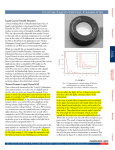
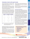
—1—
FIRS Users’ Manual
Dr. Haosheng Lin [email protected], (808)573-9538
Institute for Astronomy ATRC, University of Hawai’i
34 Ohia Ku St., Pukalani, HI 96768
Sarah Jaeggli [email protected], (808)956-5465
Institute for Astronomy, University of Hawai’i
2680 Woodlawn Dr., Honolulu, HI 96822
Lasted edited on 2010-01-04 by SJ
1. Introduction to FIRS
2. Startup Procedure
i. Kodak 2K CCD
ii. Papaya
iii. Newport Universal Motion Controller/Driver ESP 300
iv. Coconut
v. Virgo 1K Infrared Array
vi. Meadowlark Liquid Crystal Digital Interface D3040/3050
vii. Infrared Camera Hexapod
viii. High Resolution Mode Mechanized Optics
3. The FIRS Software
i. The FIRS Main GUI
ii. The Spectrograph GUI
iii. The LCVR Calibration GUI
4. Using the Instrument
i. Taking an Image
ii. Taking a Movie
iii. Taking a Single Wavelength Scan
iv. Taking a Tandem Wavelength Scan
v. Switching Wavelengths
vi. Switching Spatial Resolutions
vii. Calibration Procedures
5. Troubleshooting
6. Observing and Calibration Short Lists
7. Examples of Data
—2—
1. Introduction to FIRS
The Facility Infrared Spectropolarimeter for the Dunn Solar Telescope is an advanced imaging spectropolarimeter developed by the Institute for Astronomy - University of Hawai'i (P.I.
Haosheng Lin) and the National Solar Observatory. This instrument provides simultaneous
spectral coverage at visible and infrared wavelengths through the use of a unique dual-armed
spectrograph design. The geometry of the spectrograph has been specially designed to capture
the Fe I 6302 Å and the FeI 15648 Å or HeI 10830 Å lines with maximum efficiency. In addition,
the spectrograph operates in a multiple slit mode. By using narrow band filters, the spectra
from four consecutive slit positions can be imaged at once on the same detector. This feature
greatly reduces the time necessary to scan across a large area on the sun, making it an ideal instrument for the study of quickly developing active regions.
Telescope Beam from HOAO
Motorized Field Steering Mirror
Slit-Jaw Return Beam
95/5 Beam Splitter
Hi-res/Lo-res Optics
Grating
Fold Mirror
Slit Unit
Fold Mirror
Cylindrical Lens
Visible Arm
IR Pick-off Mirror
Lens
Vis Pick-off
Mirror
LCVR 1
LCVR 0
DWDM Filter
Fold
Mirror
Lens
Lens
LCVR 1
LCVR 0
DWDM Filter
Wollaston Prism
Focal Plane
Lens
Infrared Arm
Off-Axis Parabolic
Mirror
Wollaston Prism
Focal Plane
Figure 1. The FIRS optical path.
The current configuration of FIRS with HOAO will deliver diffraction limited observations
of the Fe I 6302 Å and Fe I 15648 Å, or the Fe I 6302 Å and He I 10830 Å solar magnetic field
diagnostics. Additional beamsplitters placed in the AO optical bench allow FIRS to share the
light path with the Interferometric Bidimensional Spectrometer (IBIS), which provides coverage
of the chromospheric Ca II 8542 Å line, and the G-band imager without interfering with FIRS
observations.
—3—
FIRS is an off-axis reflecting Littrow configuration spectrograph which can operate in an f/
36 low resolution or f/108 high resolution mode. A diagram of the current optical path is
shown in Figure 1. The DST is a 76 cm aperture vacuum tower telescope and provides a beam
which has been processed by the High Order Adaptive Optics system (Rimmele et al. 2004). A
motorized field scanning mirror and additional optics form an image on the 4-slit unit. Light
passes through the slits to an off-axis parabolic mirror which collimates the beam. The beam is
then spectrally dispersed by a 31.6 line/mm echelle grating with a 63.5º blaze. For the standard
alignment, 6302 Å has been selected from the 90th order, 15648 Å has been selected from the
36th order, and HeI 10830 Å has been selected from the 34th order; the steep blaze angle ensures that there is more light at these widely dispersed, high orders. The dispersed beam is refocused by the parabolic mirror a second time and then travels to the respective pick-off and
fold mirrors for the visible and infrared detectors and their optics. Following this point the layout of the essential optics for each arm is identical. Astigmatism is inherent in the spectrograph
due to the second reflection from off-axis paraboloid. In order to correct this astigmatism the
next focusing element is a cylindrical lens which refocuses the beam along the vertical axis. Following this there are two re-imaging lenses which readjust the size and focus of the image on
the camera. Between these two lenses are two liquid crystal variable retarders (LCVRs) which
modulate the beam polarization in an efficiency-balanced tuning scheme (and there is space for
a linear polarizer and quarter-wave plate for calibration of the LCVRs). Following the polarizers
is a DWDM, or dense wavelength-division multiplexing filter, which has been adapted from optical communications technology. This narrow filter has been made especially for each wavelength
and ensures that the spectra from adjacent slits do not overlap at the focal plane. A Wollaston
prism, or polarizing beam splitter, acts as the analyzer for the modulated beam and vertically
separates linearly polarized light into its orthogonal components, and sits immediately before
Table 1. Properties of FIRS
Property
FIRS f/36*
FIRS f/108*
Telescope
76.2 cm Solar Tower
...
Rayleigh limit @ 6302
0.21”
...
Rayleigh limit @ 10830
0.36”
...
Rayleigh limit @ 15648
0.52”
...
Field
174” x 75”
58” x 25”
Vis Spatial Sampling
0.30” x 0.08”/pix
0.10” x 0.03”/pix
IR Spatial Sampling
0.30” x 0.15”/pix
0.10” x 0.05”/pix
Nominal Scan Time**
20 min
...
6302 Spectral Resolution (Sampling)
0.03 (0.01) Å
...
10830 Spectral Resolution(Sampling)
... (0.04) Å
...
15648 Spectral Resolution (Sampling)
0.17 (0.05) Å
...
*Assuming use of a 40 μm slit
**Assuming a 5 sec scan step cadence
—4—
the final focal plane. The detector for the infrared side is a Raytheon Virgo 1024 × 1024
HgCdTe array. The detector for the visible side is a Kodak 2048 × 2048 CCD.
A raster of a solar region is produced by stepping the field scanning mirror, moving the
image across the slit unit. For a single slit position in the raster both the visible and infrared
arms obtain spectral images of each of the four polarization states provided by the LCVRs. The
Stokes vector is recreated from these four images in post-processing. This method produces
observations of the visible and infrared spectrum which are coincident in space and time with
little ambiguity (although differential refraction caused by the Earth's atmosphere can cause a
slight shift between the focused telescope image at different wavelengths). Each spectral image
consists of eight spectra, where the 4 slits have been vertically separated by the Wollaston prism
into their orthogonal polarization states. During a scan the four slits fully sample four adjacent
regions and for this reason FIRS shows a significant performance advantage over traditional single slit imaging spectrographs. The properties of the FIRS standard configuration are given in
Table 1. The result after post processing is a Stokes data cube for the visible and infrared which
contains the Stokes spectrum for each of the consecutive slit positions (for unbinned data,
roughly 1000 spatial pixels × 760 scan steps × 400 spectral pixels × 4 Stokes components for
the visible wavelength data, and 500 spatial pixels × 760 scan steps × 200 spectral pixels × 4
Stokes components for the infrared wavelength data).
2. Startup Procedure
Make sure the two main power strips are located on the underside of the FIRS main instrument table are on. Following this, the computers (Papaya and Coconut), LCVR controllers,
motion controllers, and camera controllers can be turned on. The components in the electronics chassis and the location of power switches is shown in Figure 2.
The cameras should be switched off in the evening, but the computers, LCVR controllers,
and motion controller can all be left powered on for the duration of the run. Just be sure to
check that the motion controller and LCVR controllers are still working properly the next
morning.
2.i. Kodak 2K CCD
Turn the camera on first, the power switch for the CCD is located on the end of the
power cable near the camera.
2.ii. Papaya
The computer for the Kodak 2K CCD is a dual boot system running Linux/Fedora and
Windows XP. The on/reset button for Papaya is a black square button on the front panel. Linux
is the default option upon startup and the operating system under which the camera is run, so
nothing needs to be done while the system is booting. At the end of the boot sequence the
linux terminal will prompt for the username and password (the end of the boot sequence actually results in rows of text that look like the computer is still booting, I think this is some IDL
startup garbage, just press enter and you’ll get the login prompt).
login: ******
password: ******
—5—
LCVR controller (vis)
LCVR controller (IR)
motion controller (vis)
Coconut (IR)
Papaya (vis)
Figure 2. FIRS electronics chassis, the power switches
are indicated by the red ovals.
Then at the prompt type:
[tic@papaya ~]$ startx
and Linux(xwindows) will launch. Papaya has direct control of the Port 4 calibration optics at
prime focus. The Java control gui is accessed through the ‘port4.jar’ icon on the Linux desktop.
Open a terminal window on Papaya. The camera is initialized with the following command:
[tic@papaya ~]$ ./start_firs
A few lines of output will follow ending with the IDL prompt. Next initialize the camera and
start the FIRS visible camera gui:
idl> firs
The gui will appear and if there is not yet a data folder for the current day it will create one
(and tell you that it has, click ‘ok’). From the gui take a couple of pictures to make sure the
camera is working. Try changing the exposure time and verify that the counts on the camera
change accordingly. If the counts do not change you just exit FIRS and IDL and restart from
./start_firs.
—6—
Papaya
Coconut
Kodak 2k CCD (12-bit)
Virgo 1K Array (14-bit)
Visible LCVR
Infrared LCVR
Visible Motion Controller
Infrared Camera Hexapod
Grating Rotation Stage
Hi-Res/Lo-Res Optics
Field Scanning Mirror
Linear Stage
Figure 3. Conceptual map of FIRS electronics hierarchy.
2.iii. Newport Universal Motion Controller/Driver ESP 300
The Newport motion controller attached to the visible-side operates the grating rotation
stage and the linear stage for the field scanning mirror. The stages can be moved using the buttons on the motion controller or via the FIRS gui.
Visible Motion Controller:
axis one--rotation stage, spectrograph grating
axis two--linear stage, field scanning mirror
First turn on the power for the motion controller, this is a black button on the far left of
the controller. When the controller has completed its startup the display will show three axes
and their positions (which will always be zero after startup). The axes will show that they are
‘off’ on the display. Turn the field scan mirror (axis 2) ‘on’ by pushing the button immediately to
the right of the display. The grating axis can be left off for normal observation modes. Note
that only one button can be pushed at a time on the motion controller, and you must wait until
a command is finished/an axis has stopped moving before giving another command. The field
scanning mirror should be initialized using the ‘Home axis’ button on the far right of the controller. When the FIRS gui for the visible side is running send the field mirror to its default center scan position by clicking in the “Field Scan Mir” position field and pressing enter. You should
also see the image move on the slitjaw camera display.
2.iv. Coconut
—7—
The operation of the Virgo 1K infrared array requires a Windows environment. When
Windows has finished booting simply enter the login and password. The power button on Coconut is the round dark red button.
If you intend to synchronize the camera operation using the system clock, check the
clocks on both computers and make sure that the are close (within 1/4 second). If not, force
the computer to check the default internet time server (should be accessible through the task
bar clock on both Linux and Windows). File names for the fits data are also produced using the
system clock time and it’s nice when they match between the visible and infrared data.
2.v. Virgo 1K IR Array
The camera-head electronics and power supply are external to the infrared camera dewar.
To startup the camera, the switch on the power supply needs the be switched on and the 12 V
adapter for the camera head cooling fan needs to be plugged in. If the cooling fan is left on
when the camera is off the array may show “snow” varying of hot pixels on the right side of the
image. We think this is due to static buildup on one of the AD cards, so be sure to unplug the
fan when the camera is shut down.
On the computer desktop there is a set of three icons at the top of the left-hand screen.
First launch the ‘Virgo 1K’ program (red and yellow hand icon) and turn the camera on in software via the ‘On/Off’ menu, clicking through the subsequent windows. Launch ‘Camera Program’ (cyan icons with text ‘SEIR’). Leave both of these program windows running in the background or minimized. Start IDL 6.3 using its icon and type ‘firs’ in the command line to start the
FIRS gui.
The Virgo 1K can take images at a maximum of 8 per second, so the minimum exposure
time is 125 msec and the exposure time can only be a factor of 125 msec (250, 375, 500, ect.)
2.vi. Meadowlark Optics Liquid Crystal Digital Interface D3040/3050
Flip the switch on the left of the controllers for the visible and infrared LCVRs. A green
light will come on and an amber light will blink for a moment and then turn off. The amber light
signifies that the controller is communicating with the LCVRs. If the amber light does not blink
when the polarimeter is supposed to be running, cycle the power on the controller (no system
restart necessary). After the FIRS gui has been started verify that the LCVRs are working properly by taking a test images with the polarimeter on. For the infrared FIRS gui make sure the
correct LCVR tuning is being used from the menu Polarimeter>Show LCVR settings. If a sunspot is present on the disk, place on of the slit on the sunspot, verify that polarization signals are
present in the polarized Stokes spectra (Stokes Q, U, and V).
2.vii. Infrared Camera Hexapod
The Virgo 1k dewar is enclosed by a fully motorized hexapod mount which is controlled
by Coconut via IDL (start a new IDL session and type ‘hexapod’ in the IDL command line). The
hexapod allows the user to specify the X,Y, and Z position and tilt of the array, This position has
been carefully determined and should not need to be altered. The hexapod share a power supply with the high resolution beam optics mechanics, be sure not to run both at once.
2.viii. High Resolution Mode Mechanized Optics
The optics for the high and low resolution modes are under the black chimney in front of
the slit. In low resolution mode the simply light passes through the 780 mm lens (in the white
—8—
Figure 4. The FIRS gui with Observation tab open.
housing) and is folded onto the slit, providing an f/36 beam. In high resolution mode the 780
lens is bypassed and the beam travels to a mirror at the top of the FIRS chimney that provides
an f/108 beam at the slit. The optics are mechanized and there is a switch at the slit access port
—9—
that puts the chimney fold mirrors in place(on/off switch only for emergencies, leave in the on
position). The motor is powered by the same supply as the hexapod, located under the end of
the optics table which must be turned on before use.
3. The FIRS Software
3.i. The FIRS Main GUI
The gui, shown in Figure 4, has many menus, buttons, tabs, toggle switches, and input fields.
Don’t let this fool you into thinking it is complicated. Views of the gui are shown in figures 4-7
and a brief description of all the gui commands is given in the following tables.
Menu
Sub-Menu
File>
Save Current Image
Description
Refresh Display
Show Data Disk
Shows the current data disk and usage*
Set Data Disk
Show Data Path
Set Data Path
Debug On
Debug Off
Exit
Obs>
Save Obs Parameters
Get Obs Parameter
File
Camera>
Show Camera ID
NICMOS 3
TCM2620
Kodak ES1.0
Kodak ES4.0
Kodak 2k CameraLink
the default Vis camera
—10—
Menu
Sub-Menu
Description
Virtual Camera
SEIR IK
the default IR camera
SEIR 2K
Polarimeter>
Sync>
Read/Edit LCVR File
opens a text editor where the LCVR voltage
setting can be changed
Show LCVR Settings
Prints the voltage settings for the LCVRs
Calibrate LCVR
Runs the LCVR calibration gui
Read/Edit Sync File
Show Sync Settings
Spectrograph>
Disp Range>
...
Preset configurations for the window display
ranges for intensity and the QUV components
of the Stokes vector
*A note on disk space: The gui shows the amount of disk space in the default directory on
startup and will warn you if disk space is running low, however it will not change the data disk
for you so this needs to be done manually using the menu: file> data disk.
Button
Description
Abort
Halts whatever imaging process is running after the after the most recent image has been displayed (and saved). Might need to press this a
couple of times until the gui responds.
Snapshot
Takes a single frame of data with the specified integration time (one
image for intensity or 4 images for full Stokes polarimetry)
Movie
Continuously takes images until ‘Abort’ is pressed
Burst
Takes the number of images specified by ‘Loop’, this is repeated the
number of time specified by ‘Repeat’. This is the primary observation
mode and more is described in Section 4: Setting up a Scan.
Pause
Temporarily stops a ‘Burst’ (or ‘Movie’) which can then be restarted
from the same point in the burst.
—11—
Button
Description
GetDark
Takes an image and saves it in temporary memory unless
‘Save to Disk’ is specified, this dark is used to correct the image displayed by ImExam and is essential for the LCVR calibration.
GetFlat
Takes an image and saves it in temporary memory unless ‘Save to Disk’
is specified, this image is used to flatfield the image displayed by
ImExam.
Fields
Description
Exp(ms)
The exposure length in milliseconds.
CoAdd
The number of exposures to co-add.
Loop
The number of steps in a scan observation, only relevant in burst
mode.
Repeat
The number of times to repeat the burst observations.
Mag
The magnification factor of the Imexam image display, 0.0 will scale
the image to fit on the screen, 0.5 will show the image rebinned by
1/2, 1.0 will show the image at the proper pixel size.
Message Box
Prints the output messages for processes the program is running.
Toggle
Sub-Toggle/
Field
Description
Observation Tab
Save to Disk
Saves all of the data taken to a file labeled with the date
and time in the format yyyymmdd.hhmmss.number. For a
movie or snapshot the number ending is ‘0000’, however
for burst mode all of the images in the burst are labeled
with the starting time of the burst and the number in the
loop.
Spatial/Spectral
Binning
Rebins the data in the spectral or spatial dimension by
the specified factor before saving.
Inc. Tele Hdr
Includes the telescope parameters and pointing information in the fits image header.
—12—
Figure 5. The Fits Header tabs.
—13—
Toggle
Sub-Toggle/
Field
Sync Control
Description
Synchronizes operation of the visible and IR cameras using a network handshake or timing file.
Sync Control
Mode
Polarimeter
‘Master’ and ‘Slave’ are for the network handshake
syncing. The ‘Master’ is the visible side which talks to the
motion controller and the ‘Slave’ is the IR side. ‘Timer’
uses the system clocks and a timing file to take a synchronized scan.
Turns the LCVRs on and takes full Stokes vector data, 4
frames.
ImExam Display
Selects which of the stokes vector components to display in ImExam
Feed Optics F#
Indicates which feed optics are currently in use (but does
not actually change them).
Slit Width
Input field for the width of the slit in the selected unit
Field Scan Mir
The field scanning mirror will step the distance input in
the ‘Step’ field for each observation when in Burst mode.
Ctr, Start, Step,
C Pos
Grating Scan
These fields define positions in millimeters for ‘Field Scan
Mir’. Clicking in any of these boxes and pressing enter
will send the field scanning mirror to the position value
specified. ‘Center’ is the center of the scan. ‘Start’ defines the start position of a scan, and ‘Step’ defines the
distance between scan positions. ‘C Pos’ is the position
that the stage will return to when the scan is complete.
The grating will step the distance(in degrees) specified by
the parameters in the adjacent fields when in burst
mode.
—14—
Figure 6. The Display and Multi-Slit tabs.
—15—
Toggle
Sub-Toggle/
Field
Description
Ctr Start, Step,
C Pos
These fields define positions in degrees for ‘Grating Scan.’
Clicking in any of these boxes and pressing enter will
send the grating to the position value specified. ‘Center’
is the center of the scan, and where the spectrum is centered on the detector. ‘Start’ defines the start position
of a scan, and ‘Step’ defines the distance between scan
positions(for the grating this is in degrees per unit slit
step). ‘C Pos’ is the position that the rotation stage will
return to when the scan is complete.
Fits Header Tab
Extra Headers
Additional comments about the observation that you
would like to be written into the fits header go here.
Tele. Pointing
The telescope pointing information appears in this field
when you click the “Get Tel Pointing” button.
Display Tab
De-Streaking
Set this toggle to remove streaking from the Q, U, and V
components of the Stokes vector.
Show Scan
Map
Builds a scan map based on information given in the
‘Multi-Slit’ tab.
Select
Selects the spectrum to build the map from.
Auto I Range
Automatically sets the display range of the intensity
component of the stokes vector in the ImExam data display.
Auto S Range
Automatically sets the display range of the polarized
components of the stokes vector in the ImExam data
display.
I, Q, U,V min
and max
Dark Subtract
Sets the image display range for the Stokes Display.
Applies the most recent dark to the image displayed by
ImExam, is is not applied to the data written to disk (?).
—16—
Figure 7. The Pol Calib and Alignment tabs.
—17—
Toggle
Sub-Toggle/
Field
Description
Flat Fielding
This applies the most recent flat field to the image displayed in the ImExam window, it is not applied to the
data written to disk (?)
Alignment
Grid
Overlays a grid on the displayed image for alignment of
the instrument.
Multi-Slit Tab
No. of Slits
The number of slits in the slit unit, usually 4.
Continuum
Center
The pixel index for the center of a continuum window.
Continuum
Width
The width of the continuum window in pixels.
Line Center
Position of the main line of interest, in pixels.
Line Width
Width of the line, in pixels.
IFU
nothing here for now
Pol Calib
DST Port4 LP
Places the port 4 prime focus LP in the beam for the polarimetry calibration of FIRS.
DST Port4 WP
Places the port 4 prime focus WP in the beam for calibration of FIRS
Ctr, Start, Step,
C Pos
These fields define positions in degrees for the LP or WP.
Clicking in any of these boxes and pressing enter will
send the WP to the position value specified. ‘Center’ is
the position for the center of the burst. ‘Start’ defines
the start position of a scan, and ‘Step’ defines the distance between positions. ‘C Pos’ is the position that the
rotation stage will return to when the burst is complete.
Alignment
De-Scramble
—18—
Toggle
Sub-Toggle/
Field
Description
dS
Align ImSG
x1, y1, x2, y2,
size
*’Stokes Display’ and ‘Remove Streaking’ take a little extra processor time, leave them off if it’s
necessary to run a little faster, but in general it is good to see the Stokes data so you can be
sure things are working.
Figure 8. Spectrograph GUI.
—19—
3.ii. The Spectrograph GUI
If it is necessary to change the angle the spectrograph grating, the spectrograph GUI can
be opened by selecting the desired wavelength from the ‘Spectrograph’ menu or by typing the
command ‘spectrograph’ in the IDL command line. This opens a window like the one shown in
figure 8. If the spectrograph parameters are altered push the ‘ReCalculate’ button, select the
desired order and push the ‘Goto Selected Order’ to move the grating to the new position.
The correct values for default 6302/15648 Å setup are:
grating constant: 31.6 mmˉ¹
spectrograph angle: -3.75º
wavelength: 15648 Å
grating offset: 0.0º
select 36th order, this configuration gives the 90th order of 6302 on the CCD.
3.iii. The LCVR Calibration GUI
With time and temperature changes the retardance of the LCVRs will drift. When the
drift becomes significant it is time to recalibrate the LCVRs. Calibration is done separately for
the visible and infrared. The configuration for calibration should be similar to that for solar flatfields: sun center with the telescope out of focus.
For the LCVR pair of your choice, first take a dark with the exposure length you intend to
use for the calibration using the ‘GetDark’ button. Open the LCVR calibration gui from the ‘Polarimeter’ menu. Place the linear polarizer in the beam and set the angle to 0º. There are two
LCVRs and we calibrate each separately. If it seems necessary, the LCVR which is not being
calibrated may be removed from the beam as there is sometimes significant retardance at zero
voltage. LCVR 0 is closest to the camera and LCVR 1 is furthest from the camera (or first in
the beam). To begin the calibration of LCVR 0 select it in the LCVR toggle box and set the region of the array you wish to use by entering the values into the x1, x2, y1, and y2 boxes (we
use the full extent of the bottom beam something like 0:1023, 0:500 for the IR and 0:2047,
0:1000 for the visible). The default V0=0.0, V1=10.0, and dV=0.25 are probably fine for a first
coarse calibration but change dV to 0.125 once you are confident you are going to get a good
calibration. Turn on Imexam if you want and hit the ‘Calibrate’ button. The LCVR controller is
cycling through voltages and you can see the result as rapid increase in intensity and a gradual
drop to zero (if you see the reverse you have chosen your beams backwards). When the calibration is done the intensity vs. voltage curve and its best fit will be plotted in the main window
to camera
LCVR 0
LCVR 1
LP
from telescope
—20—
Figure 9. LCVR Calibration GUI.
and the voltage values for the necessary retardances will be marked by crosses on the plot. For
a good curve all the crosses except 0º will fall on the line. A reasonable looking calibration will
look like the gui shown in figure 9.
—21—
LCVR 1 needs to be rotated by 45º just during its calibration, move the knob on the LCVR
to the top and when you are finished with the calibration be sure to move it back down to the
side. Change the LCVR toggle to ‘1’ in the gui and run the calibration as above.
After the calibration the voltage values that have been determined for the retardance need
to be entered into the tuning file. From the FIRS gui select ‘Read/Edit LCVR File‘ from the Polarimeter menu. In the default directory select ‘lcvr.tune.default’ and use the text editor to enter
the values that were printed in the output text box in the LCVR calibration gui, if you lose these
values you can reload the file from the ‘Cal_Data’ menu, these are stored separately for LCVR 0
and 1, bust pick the most recent. ‘lcvr.tune.default’ should say which values are need, enter the
voltages, save, and exit. For the new tuning file to take effect ‘Read/Edit LCVR’ file again and exit
without making any changes.
Be sure to test the new setup using the FIRS calibration linear polarizer and 1/4 waveplate
just in front of the LCVRs. The cross-talk between input Q, U, and V states should be at the
10% level or below. We are working on a fine tuning procedure to make this calibration even
better.
4. Using the Instrument
The imaging components of the FIRS spectrograph are separate and are controlled independently by each computer, however the mechanical components are not. The visible arm
computer(Papaya) controls the motion controller for the grating and slit unit so while the visible side of the spectrograph can be run separately, the infrared side must be run in tandem with
the visible side. We’ll focus first on taking images and setting up a scan using the visible side,
then we’ll consider how to use the full system.
4.i. Taking an Image
Set ‘Exp’ and ‘CoAdd’
Turn on ‘Save to Disk’ if you wish to save the image
Type in the ‘Fits Header’ if you are saving the image
Move the field scanning mirror to the desired position by typing in one of the position boxes
and pressing enter
Turn on ‘Polarimeter’ if you want a full Stokes image
Press the ‘Snapshot’ button
4.ii. Taking a Movie
This is the same as taking a single image, but images are taken continuously at a single slit position, so we recommend leaving ‘Save to Disk’ off.
Set ‘Exp’ and ‘CoAdd’
Turn on ‘Save to Disk’ if you wish to save the images
Type in the ‘Fits Header’ if you are saving images
Move the field scanning mirror to the desired position by typing in one of the position boxes
and pressing enter
Turn on the ‘Polarimeter’ if you want a full Stokes image
Press the ‘Movie’ button
Press the ‘Abort’ button to stop the movie
—22—
4.iii. Taking a Single Wavelength Scan (visible)
Set ‘Exp’, ‘CoAdd’
Turn on ‘Save to Disk’
Set slit scan ‘Step’
Set ‘Loop’
Turn on ‘Slit Scan’
Set slit scan ‘Ctr’
Set ‘Start’ position for the slit scan
Set ‘Step’
Turn on ‘Polarimeter’ for full Stokes data
Type ‘Fits Header’ and ‘get telescope pointing’
Press the ‘Burst’ button to start the scan
FIRS has a variety of slits to pick from, they are listed in Table 2. The size of the scan step
and number of steps in a scan can be adjusted arbitrarily, however to achieve optimal sampling
we have set the step size equal to the slit width. For a fully sampled field using the 30 or 40 μm
slit the parameters should be set as follows:
scan step = 0.030, 0.040 μm
loop = 190, 145
scan center = 12, 12 mm
start = 9.15, 9.12 mm
Table 2. Available Slit Units
Slit Name
Number of Slits Slit Width (μm)
Slit Length (mm)
Slit Spacing (mm)
15 μm short
4
15
10.0
5.70
15 μm long
4
15
20.48
5.70
30 μm short
4
30
10.0
5.70
30 μm long
4
30
20.48
5.70
30 μm double
2
30
20.48
11.4
40 μm single
1
40
20.48
---
40 μm long
4
40
20.48
5.80
4.iv. Taking a Tandem Wavelength Scan (dual visible and infrared)
There are two modes which allow the visible and infrared camera systems to take observations as a coordinated scan. For ‘Timer’ mode both computers wait for a specific time to
start an observation. A timing file set from the ‘Sync’ menu contains the seconds at which new
observations are begun and when an observation finishes it waits until the next second specified in the timing file. For 5 second timing observations are started at the beginning of the next
—23—
Table 3. Scan Step Optimization
Slit
Number of Scan Steps
4 slit, 15 μm
380
4 slit, 30 μm
190
2 slit, 30 μm
380
1 slit, 40 μm
---
4 slit, 40 μm
145
minute after ‘Burst’ is pushed and are taken at 0, 5, 10, 15, 20, 25, 30, 35, 40, 45, 50, and 55 seconds for each minute until the end of the burst. Both computers are effectively running separately so it is important to set the exposure and co-add such that the observations for the visible and infrared side take about the same amount of time (this may seem easy but in practice it
takes a couple of tests to get the right timing down, the exposure and co-add will of course be
different for the visible and infrared cameras). This is also why the system time for each computer must be set accurately.
For ‘Master’ and ‘Slave’ mode the computers are coordinated through a network connection and when an observation finishes on one computer it will wait for the other computer to
finish its observation before starting the next one. No special timing is necessary and the exposure length and co-add can be set as desired. This mode is preferable and runs faster than
‘Timer’ mode. The ‘Master’ is the visible-side computer which controls the field scanning mirror
and the ‘Slave’ is the infrared-side computer.
For the (Master) visible side:
Set ‘Exp’, ‘CoAdd’, and ‘Loop’
Turn on ‘Save to Disk’
Set ‘Spatial/Spectral Binning’ factor
Turn on ‘Sync Control’, set ‘Master’
or set ‘Timer’ and load a timing file via the ‘Sync’ menu
Turn on ‘Field Scan Mir’
Set the ‘Ctr’, ‘Start’, and ‘Step’
Turn on ‘Polarimeter’
Turn on ‘Inc. Tele Hdr’
Type ‘Fits Header’ comments
Press the ‘Burst’ button to start the scan
For the (Slave) infrared side:
set ‘Exp’, ‘CoAdd’, and ‘Loop’
turn on ‘Save to Disk’
Turn on ‘Sync Control’, set ‘Slave’
or set ‘Timer’ and load a timing file via the ‘Sync’ menu
—24—
turn on ‘Polarimeter’
type ‘Fits Header’ comments
press the ‘Burst’ button to start the scan
Repeating a Scan:
The ‘Repeat’ field makes it possible to repeat a scan many times over a long period. This is
only recommended when the seeing is fair and stable. When the seeing conditions are more
erratic it is important leave time between scans to get a new AO flat field so that the image
resolution is optimal during observations.
4.v. Switching Wavelengths
The infrared arm of FIRS can swap between He I 1083 and Fe I 1565 nm modes by changing a few optics and software settings. Switch off the power to the IR LCVR controller. On the
IR side of the FIRS optical bench add/remove:
For Fe I 1565 nm:
1565 nm DWDM filter
1565 nm blocking filter
1565 nm LCVRs (and swap cables)
For He I 1083 nm:
1083 nm DWDM
1083 nm LCVRs (and swap cables)
Move the final lens before the camera to the position indicated in the bench using the digital
micrometers. Finally, in the FIRS IR gui change the LCVR tuning file, selecting in the menu Polarimeter> Read/Edit LCVR File. Select the proper lcvr.tune.default file for the wavelength. Then
turn the LCVR controller back on and verify that it is working.
4.vi. Switching Spatial Resolution
To switch from low to high resolution optics (or vice versa), make sure the power supply
for the F/108 mirror tower is turned on. Switch the power on the F/108 mirror tower controller to 'ON'. In the FIRS gui set the “high res/low res” toggle switch on the F/108 mirror tower
controller to select the resolution mode. Note: The field scan mirror scan step and scan starting position will be scaled automatically by the software.
4.vii. Calibration Procedures
Flat Fields
Solar flats are produced from a full Stokes spectra taken at disk center with the AO mirror
un-flat and random guiding. Flats should be taken every couple of scans and before swapping
between 1083 and 1565 nm. The slits should be as evenly illuminated as possible, with the scanning mirror at the center the field. Exposure time and co-add for the solar flat should be the
same as the data.
For either a solar or lamp flat:
set ‘Exp’ and ‘CoAdd’
—25—
set ‘Loop’, (16)
set the ‘Field Scan Mir’ to the center
turn on ‘Save to Disk’
turn ‘Polarimeter’ on
type ‘Fits Header’ comments
push the ‘Burst’ button to start the sequence of flat fields
Note: Lamp flats can be taken with the flat field lamp located under the FIRS optical table. The
lamp is connected by a large core fiber optic to a collimator and a set of fold mirrors places the
light on the slit. The last fold mirror must be slid into place (otherwise it would block the solar
beam) and there are three kinematic pushers on the table for its positioning. If the lamp is on
and the final mirror is not in place the whole AO bench is illuminated so be careful if calibrations are being done for another instrument. The lamp is about half as bright as the sun in the
IR and about 1/4 times as bright for the visible, so chose an integration time 2-4 times that for
the data. The lamp has an uneven illumination pattern so I have not found it very useful for flatfielding the data.
Darks
With the dark slide in place take a burst at the default slit position with the exposure
length of the data and flat field scans.
set ‘Exp’ and ‘CoAdd’, same as for the data, flat field, and calibration images
set ‘Loop’, (16)
turn ‘Save to Disk’ on
‘Polarimeter’ off
type ‘Fits Header’ comments
push the ‘Burst’ button to start the sequence of darks
Polarimetry Calibration
The LCVRs change with operation time and temperature so it is important to obtain a
new calibration every few hours during observations. A well sampled polarization curve with
10º sampling will lead to a more accurate polarization calibration. The motorized optics at the
DST Port 4 prime focus are available for this purpose. There are also calibration optics which
can be put in place immediately before the LCVRs in each arm of FIRS and must be adjusted by
hand, although these calibration optics may become motorized in the future.
When using either set of calibration optics the procedure will be:
set the LP (linear polarizer) to 0º
cycle the WP (1/4 wave plate) through 360º using 10º increments or better
take full Stokes observations at each position
Papaya has direct control of the Port 4 calibration optics at prime focus. The Java control gui is
accessed through the ‘port4.jar’ icon on the Linux desktop. The polarization calibration data can
also be set up to run automatically using the FIRS gui. The ‘Pol Claib’ tab is used to set up a
calibration burst:
—26—
put the ‘DST Port 4 LP’ in with ‘Ctr’=0, ‘Start’=0, and ‘Step’=0
put the ‘DST Port 4 WP’ in with ‘Ctr’=180, ‘Start’=0, and ‘Step’=10
turn on ‘Save to Disk’
set ‘Binning’ same as for the data
turn on ‘Inc. Tele Hdr’
type ‘Fits Header’ comments
turn on ‘Polarimeter’
push ‘Burst’
Note about FIRS polarizers: The infrared side linear polarizer is off by about 10º, ie 10º on the
scale = 0º actually
5. Troubleshooting
IDL
If IDL becomes unresponsive try entering the command ‘retall’ in the IDL command line a
few times. If it does not recover after this restart it in the same way as for the startup procedure.
Imexam
If Imexam becomes frozen, close any offending windows and type ‘retall’ in IDL command line and redisplay the last image by typing ‘imexam, image’.
LCVR Controllers
The amber light signifies that the controller is communicating with the LCVRs. If the amber light does not blink when the polarimeter is supposed to be running, cycle the power on
the controller (no other hardware or software restart is necessary).
LCVR tuning
If the stokes vector for the IR does not look right (check against example data) and the
LCVR controller is working, you may be using the wrong tuning file. Try swapping it from the
menu using Polarimeter>Read/Edit LCVR File
Newport Motion Controller
Sometimes the communications between Papaya and the motion controller hang. Turn off
the motion controller power and try typing ‘retall’ in the terminal running IDL (if this doesn’t
work exit IDL restart the FIRS software from ./start_firs). Power on an initialize the motion
controller and try again.
If a controller error occurs during operation(limit switch ect.) the controller will emit a
loud beep and an ‘E’ will appear in the upper left corner of the display. This error needs to be
cleared before the controller can be used again, either by navigating the menu or cycling the
power on the controller.
Virgo 1K Array
If the cooling fan is left on when the camera is off the array may show “snow” varying of
hot pixels on the right side of the image in I, and looks even worse for Q, U, and V. We think
—27—
this is due to static buildup on one of the AD cards.
6. Observing and Calibration Short Lists
After reading everything in the preceding sections you should have a very good handle on
how the spectrograph operates. The short lists that follow summarize the procedures for
startup, shutdown, and operation.
Startup for FIRS Visible
Turn the power on for:
Kodak 2K camera
visible computer, Papaya
visible LCVR controller
Following computer startup:
use the login and password
type ‘startx’ at the prompt
Start FIRS
open a terminal and type:
./start_firs
idl> firs
Turn the power on for:
Newport motion controller
Initialize the motion controller:
turn axis 2 ‘on’ (field scanning mirror)
‘home’ axis 2
In the FIRS visible gui verify:
communication with field scanning mirror
communication with LCVR
camera exposure times
Short Startup for FIRS Infrared
Turn the power on for:
IR computer, Coconut
IR LCVR controller
Virgo 1K camera power supply
plug in Virgo camera-head fan power
Following computer startup:
use the login and password
Start FIRS
FIRS program icons are at the top of the screen:
start ‘Virgo 1k’, turn the camera on via the menu and click through the boxes
start ‘Camera 2.9’
start ‘IDL’ then ‘idl> firs’
In the FIRS infrared gui verify communication with:
LCVR
—28—
Short Shutdown for FIRS Visible
Exit the FIRS gui, close all windows, shutdown Papaya
Turn everything off
Short Shutdown for FIRS Infrared
Exit the FIRS gui
in ‘SEIR Camera’ click the exit button
in ‘CamIRa - Virgo 1k x 1k’ program turn camera off using ‘On/Off > Off’ in the menu
exit using the menu ‘File > Exit’
turn off camera head power
unplug 12 V adapter for camera head fan!!
Observations
set ‘Exp’
set ‘Co-Add’
set ‘Loop’(number of steps in scan)
‘Save to Disk’ on
‘Inc. Tele Hdr.’ on
‘Sync Control’ on for a tandem scan and ‘Master’ or ‘Slave’ set appropriately
‘Polarimeter’ on
‘Feed Optics’ set correctly for f/36 or f/108
‘Field Scan Mir’ on, check positions
write ‘Fits Header’ comments
push ‘Burst’
Parameters for Full-Field Scan, F/36 Mode, ~ 10 sec/step (25 min) DEFAULT
Camera
Fe I 630 nm
Exposure Time (msec) 350
CoAdd
Loop
Repeat
Fe I 1565 nm
He I 10830
125
250
2
3
2
145
145
145
1
1
1
Deep Integration, F/36 Mode, ~16 sec/step (10 min)
Camera
Fe I 630 nm
Exposure Time (msec) 350
Fe I 1565 nm
He I 10830
125
250
CoAdd
6
8
2
Loop
32
32
32
—29—
Camera
Repeat
Fe I 630 nm
1
Fe I 1565 nm
1
He I 10830
1
Deep Integration F/108 Mode ~30 sec/step (16 min)
Camera
Fe I 630 nm
Exposure Time (msec) 500
Fe I 1565 nm
He I 10830
500
500
CoAdd
6
8
8
Loop
32
32
32
Repeat
1
1
1
Polarimeter Calibration
With the same parameters as the data
Disk center, AO mirror un-flat
In the ‘Pol Calib’ tab:
DST Port4 LP ‘in’, Ctr 0, Start 0, Step 0, Cpos 0
DST Port4 WP ‘in’, Ctr 180, Start 0, Step 10.0, Cpos 0
Set Loop to 36
push ‘Burst’
Flatfields
Disk center, AO mirror un-flat, random guider
Same exposure time and co-add as the data
Darks
Put Port 4 dark in
Same exposure time and co-add as the data and flat fields
Grids and Targets
Disk center, AO mirror un-flat
Take a grid and target scan as you would a data scan, at least once per run.
Suggested Observing Cadence:
scan, scan, flat, dark, pol cal
swap wavelengths (if desired)
scan, scan, flat, dark, pol cal
7. Examples of Data
On the next few pages we’ve included some samples of raw data with labels.
Ti
I
?
I
ge
ed
.15
.25
30
30
I6
nm
nm
es
lin
ge
ed
I6
er
filt
Fe
Fe
er
filt
ic
lur
tel
1.7
2.5
g=
g=
—30—
Fe I 630.2 nm:
Q
U
V
I
}
}
I
er
filt
Na
nm
ge
s
es
3.0
lin
ed
ic
lur
tel
08
I1
s
2.7
08
ge
ed
I1
He
Si
er
filt
g=
1.5
—31—
He I 1083 nm:
Q
U
V
OH
sp
ot
in
su
n
er
I
48
.5
ge
52
.9
ed
56
56
ge
ed
I1
I1
filt
Fe
Fe
er
filt
.5
g=
1
g=
3
—32—
Fe I 1565 nm:
Q
U
V