Download DISEÑO Y CARACTERIZACIÓN DE UN

Facultad
de
Ciencias
DISEÑO Y CARACTERIZACIÓN DE UN
ESPECTROPOLARÍMETRO DE IMAGEN
(Design and characterization of an imaging
spectropolarimeter)
Trabajo de Fin de Grado
para acceder al
GRADO EN FÍSICA
Autor: Andrea Fernández Pérez
Director: José María Saiz Vega
Co-Director: Juan Marcos Sanz Casado
Septiembre-2014
2
3
Agradecimientos
Quiero expresar mi agradecimiento:
A Chema y Juanma, por su tiempo, ayuda y consejos,
al equipo de The Zia Lab por la experiencia vivida
y a mi familia y amigos por su apoyo.
4
5
INDEX
0. PREFACE ................................................................................................................................ 8
0.1. Abstract and key words ....................................................................................................... 8
BLOCK I
1. INTRODUCTION ............................................................................................................... 10
1.1. Objectives................................................................................................................................ 11
1.2. Work Scheme ....................................................................................................................... 11
2. THEORY ............................................................................................................................. 13
2.1. Maxwell’s Equations ............................................................................................................ 14
2.2. Polarized Light ...................................................................................................................... 15
2.3. Polarimetry ............................................................................................................................. 15
2.3.1. Jones Formalism ........................................................................................................ 15
2.3.2. Mueller-Stokes Formalism .................................................................................... 16
2.4. Supercontinuum spectrum generation ...................................................................... 18
2.5. Diffraction Grating............................................................................................................... 20
2.5.1. Blaze Grating .............................................................................................................. 21
3. EXPERIMENTAL SETUP ................................................................................................ 23
3.1. Dual Rotating Compensator Polarimeter ................................................................... 23
3.1.1. Boot protocol and calibration ............................................................................. 24
3.2. Supercontinuum Laser ...................................................................................................... 25
3.3. Final setup .............................................................................................................................. 27
4. RESULTS ............................................................................................................................ 31
4.1. Monochromator characterization ................................................................................ 31
4.1.1. Spectrometer calibration ...................................................................................... 31
4.1.2. Wavelength selection ............................................................................................. 33
4.1.3. Diaphragm aperture ............................................................................................... 35
4.2. Reproducibility of results ............................................................................................... 36
4.3. DRCP calibrations at different wavelengths ............................................................. 39
4.1.1. Study of a linear polarizer .................................................................................... 40
5. CONCLUSIONS AND FUTURE WORK ......................................................................... 42
6. BIBLIOGRAPHY ............................................................................................................... 44
6
BLOCK II
1. INTRODUCTION ............................................................................................................... 47
2. TASKS ................................................................................................................................. 48
2.1. Daily life .................................................................................................................................. 48
2.2. Compulsory training courses ......................................................................................... 48
2.3. Movement of a rotating stage using Matlab Executable (Mex) files ............... 49
3. BIBLIOGRAPHY ............................................................................................................... 51
7
8
0. PREFACE
The present final degree project has been carried out at two different Universities
and departments. The work done in each place is independent and about different
topics. Therefore, this work is divided into two main parts or blocks corresponding
to the work realized in each place.
Block I describes the work done at the University of Cantabria, which is the main
part of the final degree project. It was developed during the months of February to
early June at the Optics Department, under the supervision of Jose María Saiz Vega
and Juan Marcos Sanz Casado.
Block II summarizes the part of the work carried out at the University of Brown
(Providence, EE.UU). This block is a complement because of the internship
program done at the School of Engineering from June 15 to August 8 under the
direction of Prof. Rashid Zia.
0.1. Abstract and key words
Resumen
La espectropolarimetría tiene como objetivo el análisis simultáneo del espectro y
la polarización de la luz.
El propósito de este proyecto es transformar el polarímetro dinámico de imagen,
presente en el laboratorio de óptica del Departamento de Física Aplicada de la
Universidad de Cantabria, en un espectropolarímetro de imagen. Se instalará una
fuente laser de supercontinuo, desarrollando y caracterizando un monocromador
que permita seleccionar, de manera automática, la longitud de de onda deseada
dentro del espectro visible. Posteriormente, se calibrará el funcionamiento
conjunto de todo el sistema. De esta manera, seremos capaces de estudiar la
polarización de la luz y de realizar medidas de la matriz de Mueller a diferentes
longitudes de onda.
Para lograr este objetivo, el espectro continuo será separado angularmente en las
diferentes longitudes de onda mediante una red de difracción situada en una
plataforma giratoria. A continuación, se seleccionará una parte del espectro con un
diafragma. Finalmente, el polarímetro de imagen, junto con la nueva fuente, será
calibrado y puesto a prueba sobre algún elemento óptico.
Palabras clave: espectropolarimetría, polarímetro, matriz de Mueller, vector de
Stokes, red de difracción, monocromador, supercontinuo.
9
Abstract
The simultaneous analysis of the spectrum and state of polarization of light is
usually referred to as spectropolarimetry.
The main objective of this project is to transform the imaging dynamic polarimeter
located at the optics laboratory of the Departamento de Física Aplicada at
Universidad de Cantabria, into an imaging spectropolarimeter. This project aims to
implement a new supercontinuum laser source and to develop and characterize a
monochromator which will allow selecting the operating wavelength in an
automated way. The whole setup will be calibrated in a later stage. Thus, we will be
able to study the polarization of light and to perform measurements of the Mueller
matrix at different wavelengths, in a wide range of the visible spectrum.
In order to do that, the continuous spectrum will be angularly dispersed by a
diffraction grating placed on a rotating platform. Then, a fraction of the spectrum
will be selected by means of a diaphragm.
The imaging polarimeter, working with this fully characterized spectral source,
will be calibrated and tested on basic optical elements.
Key words: spectropolarimetry, polarimeter, Mueller matrix, Stokes vector,
diffraction grating, monochromator, supercontinuum spectrum.
10
BLOCK I
1. INTRODUCTION
Spectropolarimetry consists in the simultaneous analysis of the spectrum and state
of polarization of light. This analysis is of great interest when we study the
interaction of light with a system that both affects its polarization and shows a
spectral dependence.
This technique is widely used for many purposes in fields such as astronomy,
medicine, biology or chemistry.
When light interacts with matter it may suffer reflection, refraction, absorption,
scattering, dispersion or transmission. These processes can affect the state of
polarization of the light and have an effect on the polarization of the overall
transmittance, reflectance or absorption of the system.
Because the interaction may be spectrally selective, polarimetry combines with
spectral analysis to produce spectropolarimetry.
Spectropolarimetry is used, for example, to study the atmosphere and to find
biosignatures in exoplanets [1, 2]. This is possible because when light, that comes
from a star, is reflected in a planet, it acquires a certain degree of polarization. This
process is related to the interaction of light with the planet's atmosphere and,
therefore, with its chemical components.
Also, spectropolarimetry is used to study magnetic fields in stars, black holes,
active galaxies, etc… [3] since they polarize the light in different ways too.
Other fields where this technique is applied are remote sensing [4], to study fields,
tides, or the movement of glaciers; or chemistry, alimentation or quality control,
since certain molecules, called chiral molecules, have optical activity (rotate the
plane of polarization) [5]. So the analysis with light can be useful to determinate
the concentration of certain substances.
Moreover, in the last ten years, these techniques have found applications on the
medical field mainly because of their non invasive character. For example,
spectropolarimetry can be used to study biological tissues and cells suspensions
[6, 7] because the state and degree of polarization of light can give information
about the composition or the structure of a tissue.
11
1.1. Objectives
The main objective of this project is to transform the imaging dynamic polarimeter
located at the optics laboratory, into a spectropolarimeter.
The dynamic polarimeter was developed by Juan Marcos Sanz Casado during his
doctoral thesis [8]. Recently, the setup has been improved twice, the first time by
Cristina Extremiana [9] and the second by Francesco Carmagnola [10], by
implementing, respectively, a discrete wavelength source and an imaging system
on a monochromatic basis.
In that stage, the polarimeter worked with a He-Ne laser source which only allows
single wavelength measurements. The problems derived from the first spectralsource attempt (instability, cooling problems, discrete offer of wavelengths, high
power variations among lines) ended with the implementation of a
supercontinuum laser as a spectral source.
Then, this project aims to replace the He-Ne source by a supercontinuum laser and
to develop and characterize a monochromator which will allow selecting the
wavelength from the visible continuum spectrum. This way, we will be able to
study the polarization of light and to perform measurements of the Mueller matrix
at different wavelengths, in a wide range of the visible spectrum.
In order to do that, the continuous spectrum provided by the new laser source will
be angularly separated in the different wavelength by a diffraction grating. Then, a
fraction of the spectrum will be selected by means of a diaphragm. The grating will
be placed in a rotating platform controlled by a PC so different wavelengths can be
selected in an automated way. The spectral width of the transmitted beam will also
be expressed as a function of the diaphragm.
The imaging polarimeter, working with this fully characterized spectral source,
will be calibrated and tested on samples consisting on optical elements like
retarders or polarizers.
1.2. Work scheme
From here, the work is divided into four sections.
Section 2 presents the basic theory and concepts and the theory on
electromagnetism and polarimetry necessary to understand and develop the
current project.
12
Section 3 describes the experimental set up used to perform the measurements. In
this section the three main parts of the experimental set up are fully detailed:
polarimeter, supercontinuum laser source and the monochromator system.
Section 4 shows the main results. In first place, those corresponding to the source
characterization and then, the polarimeter test ones.
Finally, section 5 is devoted to summarize the tasks carried out and to indicate
future working lines.
13
2. THEORY
2.1. Maxwell's equations
Maxwell’s equations describe the propagation of an optical field in a medium [11]:
D = 
E = -
B
t
B = 0
H = J +
(2.1)
D
t
Where E and H are the electric and magnetic field, B is the magnetic induction (B =
μH), D is the electric displacement field, J is the density of current (J = σE) and ρ is
density of charge.
D and B are related to E and H by the equations:
D   0E  P
H=
B
0
M
(2.2)
(2.3)
Where P and M are the electric polarization and the magnetization, ε0 is the
vacuum permittivity and μ0 is the vacuum permeability.
From Maxwell’s equations together with relations (2.2) and (2.3), the wave
equations for E and B in a linear medium can be obtained:
 2E
0
t 2
(2.4)
 2B
 B   2  0
t
(2.5)
 2E  
2
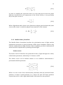
Where ε is the electrical permittivity and μ is the magnetic permeability and they
are related to the speed of light c by the equation:
1
  0 0
c2
(2.6)
14
2.2. Polarized light
The polarization is postulated as a transverse property of light. When the electric
field E of a light beam oscillates in a fully predictable way, we say that the light is
polarized. For instance, if E is contained in a plane we say that the light is linearly
polarized.
Light can be polarized in other ways: circular or elliptical in such a way that light
beam can be totally polarized, partially polarized or even fully depolarized.
Electric field can be separated into three components in the three directions of
space. For a polarized beam, if an electric field of amplitude A propagates in the z
direction with wave number k and angular frequency ω, then the equations of the
electric field components are [12]:
Ex  t   Ax cos t  kz  x 
Ey  t   Ay cos t  kz   y 
(2.7)
Ez  t   0
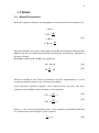
In the general case, the projection of the electric field in a plane perpendicular to
the direction of propagation is an ellipse, the polarization ellipse (figure 2.1). This
ellipse is given by the equation:
Ex2  t  E y2  t  2 Ex  t  E y  t  cos  


 sin 2  
Ax2
Ay2
Ax Ay
(2.8)
Therefore, in the plane z = 0:
Ex  t   Ax cos t 
(2.9)
Ey  t   Ay cos t   
Where φ is the phase difference between the two components:
  x   y
(2.10)
15
Figure 2.1: polarization ellipse. Ex and Ey are the components of the electric field E. Ax
and Ay are the amplitudes in x and y directions. Z is the direction of propagation.
2.3. Polarimetry
Polarimetry studies the polarization of electromagnetic waves. In order to do that,
we need an appropriate formalism to describe the state of polarization of light.
If the light is totally polarized we will use the Jones formalism. However, if the light
is partially polarized this formalism will not be enough so that the Mueller-Stokes
formalism is needed [13, 14].
2.3.1. Jones formalism:
Totally polarized light can be expressed by means of the Jones calculus developed
by R. C. Jones in 1941.
Any polarized state of light can be described by a 2x1 Jones vector and the action of
an optical element over the light can be described by a 2x2 Jones matrix.
Assuming light propagates in z direction, following Jones formalism, light can be
expressed in terms of its electric field E, with components in the x and y directions.
Each one has amplitude and phase so that the Jones vector is:
16
i
 Ex   Ax e x 
J      i y 
 E y   Ay e 
(2.11)
In order to simplify the expression above we only take into account the phase
difference between the two components of the electric field φ, as we previously
did, so the Jones vector is:
 Ax 
J   i 
 Ay e 
(2.12)
When a light beam with a Jones vector J interacts with an optical element the Jones
vector at the exit, J’, is related to J by the Jones matrix T of the element.
t 
t
J' = TJ =  11 12  J
t21 t22 
(2.13)
2.3.2. Mueller-Stokes formalism
The Mueller-Stokes formalism describes the polarization state of light and the
polarization properties of optical elements. Unlike Jones formalism, which is only
valid for totally polarized light, Mueller-Stokes formalism provides a mathematical
model useful for unpolarized or partially polarized light.
- Stokes vector:
The Stokes vector S describes the polarization state of light through four values,
called Stokes parameters, defined by G. G. Stokes in 1852.
The Stokes vector can be defined relative to six irradiance measurements I
performed with ideal polarizer.
 s0   I 0  I 90 
s   I  I 
S =  1    0 90 
 s2   I 45  I135 
  

 s3   I R  I L 
(2.14)
Where I0 is the result of the measurement performed with an horizontal linear
polarizer, I90 with a vertical polarizer, I45,135 with a 45º and 135º linear polarizer
respectively and IR,L with a right handed and a left handed circular polarizer.
17
The total intensity of light is: I = I0 + I90 = s0.
From this vector, the following polarization parameters are defined: total flux or
intensity I, degree of polarization P, degree of linear polarization PL and degree of
circular polarization PC.
I  s0
P
s12  s22  s32
s0
s12  s22
PL 
s0
PC 
s3
s0
(2.15)
(2.16)
(2.17)
(2.18)
A totally polarized beam has P = 1 and a partially polarized beam has P < 1.
Another way of write the Stokes vector is:
*
*
2
2
 s0   Ex Ex  E y E y   Ax  Ay 


*
*


s 
2
2
 Ex Ex  E y E y   Ax  Ay 
1

S=


*
*
 s2   Ex E y  E y Ex   2 Ax Ay cos  
 

  
*
*
 s3  i  Ex E y  E y Ex    2 Ax Ay sin  
(2.19)
The Stokes vector for a partially polarized beam can be represented as a
superposition of a completely polarized Stokes vector SP and a completely
unpolarized Stokes vector SU.
 s0 
 1 
1 
s 
s / s 
0
1
1
0


S=
 S P  S U  s0 P
 1  P  s0  
 s2 
 s2 / s0 
0
 


 
0
 s3 
 s3 / s0 
(2.20)
18
- Mueller matrix
The Mueller matrix M is a 4x4 matrix with real elements that represents the effect
of an optical device over the polarization state of the light. It was developed in
1943 by Hans Mueller. This matrix transforms an incident Stokes vector S into the
exiting Stokes vector S’.
 s '0 
 m00
s' 
m
1

S' =
 MS   10
 s '2 
 m20
 

 s '3 
 m30
m01
m02
m11 m12
m21 m22
m31 m32
m03   s0 
m13   s1 
m23   s2 
 
m33   s3 
(2.21)
The Mueller matrix fully characterizes a medium for a given wavelength and a
geometrical configuration because it contains within its elements all of the
polarization properties.
The difficulty of a Mueller matrix analysis is double: first we need to obtain a
reliable matrix, and then we have to analyze it in a proper way. For example the
Mueller matrix can be decomposed in several matrices each of one represents
independent physical actions of the system (diattenuation, retardation and
depolarization), thought this process is out of the scope of this work.
Any Mueller matrix can be written in the form [15]:
 1 DT 
M  m00 

P m 
(2.22)
Where DT is the transposed diattenuation vector, P is the polarizance vector and m
is a 3x3 matrix related with the optical activity of the medium.
Finally, if the light beam passes through several optical elements the resulting
Mueller matrix MT is the product of the matrices of each element in reverse order.
MT  Mn Mn-1 ...M2M1
2.4. Supercontinuum spectrum generation
(2.23)
19
The supercontinuum spectrum is achieved by propagating ultrashort laser pulses
though the highly nonlinear optical fiber. Optical fiber becomes a nonlinear
medium when high power is propagated through it.
Due to these high pulse-peak powers and high nonlinearity within the fiber, the
pulses experience large spectral broadening.
This frequency broadening was first achieved by R. Alfano in 1969 when he
propagated picosecond pulses through several materials as calcite and quartz. [16]
A nonlinear medium is a medium where the polarization vector P does not change
linearly with the electric field E.
In this type of medium, the relation between P and E can be expressed as a Taylor
series expansion [17]:
P   0  E   0  (2)E2   0  (3)E3  ...
(2.24)
Where the coefficients χ(n) are the n-th order susceptibilities of the medium.
In nonlinear mediums several effects are produced. They can be classified in two
types:
- Elastic effects: there is no energy exchange between the electric field and
the material medium. They occur through nonlinear modification of the refractive
index of the material. Some of these effects are Four Wave Mixing (FWM), CrossPhase Modulation (XPM) or Self-Phase Modulation (SPM).
- Inelastic effects: there is energy exchange between the field and the
medium. The interaction happens through modification in the material
polarizability associated with vibration of the atoms in the lattice. Some of these
effects are Stimulated Raman Scattering (SRS) and Stimulated Brillouin Scattering
(SBS).
Of course, together with nonlinear effects, there are also linear effects as chromatic
dispersion and group velocity dispersion (GVD). Chromatic dispersion is the
frequency dependence of the refractive index n(ω) of the fiber.
GVD is the frequency dependency of the group velocity in a medium which causes
pulses to enlarge in time.
So, when the short pulses propagate through the fiber, linear and nonlinear effects
affect to the shape and spectrum of the pulses.
As optical fibers are principally made of silica, which has an inversion center, the
second order nonlinear effects are neglected as the second order susceptibilities is
20
zero. As a result, the nonlinear effects in optical fibers originate from the third
order susceptibility, which is responsible for phenomena such as third-harmonic
generation, four-wave mixing and nonlinear refraction.
On the other hand, higher order nonlinear effects can be neglected because they
are very small.
2.5. Diffraction grating
A diffraction grating is an optical element with a periodic pattern (grooves or slits)
which diffract the light incident on it. There are reflective and transmission
gratings.
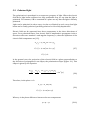
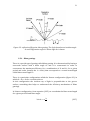
Light incident on a grating (figure 2.2) suffers diffraction in each element of the
grating. So, in principle, a beam of white light incident on a grating will be spread
in all direction. Due to the periodicity of the diffracting element, all diffracted
waves are similar and phase-shifted, being the shift related to the period of the
grating and the direction of the output beam.
In most directions light suffers destructive interference but in some directions the
slits are multiples of 2π and the interference is constructive. These directions are
called diffraction orders.
The equation that governs the direction of the diffractive rays, for the case
depicted in figure 2.2, is [18]:
sin  m   sin i  m

d
(2.25)
Where θi is the incident angle, θm is the diffracted angle, m is the diffraction order
(m = 0, 1, 2 …), λ is the wavelength and d is the period of the grating.
The resolving power R of a diffraction grating is a measure of its ability to separate
adjacent spectral lines of average wavelength λ and is given by the equation:
R

 mN  mkW

(2.26)
Where m is the diffraction order, k is the groove density, N is the number of
grooves illuminated, W is the illuminated width, λ is the wavelength and ∆λ is the
limit of resolution or smallest resolvable wavelength difference.
21
Figure 2.2: reflective diffraction blaze grating. The light beam has an incident angle
θi and a diffraction angle θm. Blaze angle θB is shown.
2.5.1. Blaze grating:
There is a special type of grating called blaze grating. It is characterized by having a
saw-tooth surface with a blaze angle θB and it is constructed in order to
concentrate the maximum efficiency for a combination of θi and θm, for a given
period and order (usually the 1st order) that correspond to a certain wavelength
called blaze wavelength λB.
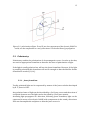
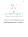
There is a particular configuration called the Littrow configuration (figure 2.3) in
which θi = θm = θB for a certain order m.
In this configuration the incident ray of light is perpendicular to the groove
surface, something that helps to understand the efficiency mechanism of Blaze
gratings.
In Littrow configuration, from equation (2.25) we can obtain the blaze wavelength
for a given period d and blaze angle.
2sin  B  m
B
d
(2.27)
22
Figure 2.3: blaze grating in Littrow configuration. θi is the incident angle, θm is the
diffraction angle, θB is the blaze angle and d is the period of the grating.
The diffraction grating used in this project is a 12.7x12.7x6 mm blaze grating made
by Thorlabs [19]. Its groove density is k = 1800 g/mm (d = 555.55 nm) and it has a
blaze wavelength of λB = 500 nm and a Blaze angle θB = 26º 44’ . The grating has a
dispersion of 0.5 nm/mrad and a damage threshold of 40 W/cm2. It is going to be
used in order to expand the continuum and separate the different wavelengths.
23
3. EXPERIMENTAL SETUP
3.1. Dual Rotating Compensator Polarimeter (DRCP)
The main instrument used is the Dynamic Rotating Compensator Polarimeter
(DRCP) (figure 3.1) located in the Optics laboratory at the Universidad de
Cantabria. This device was developed by Juan Marcos Sanz Casado. Moreover, the
device has been recently improved by Francesco Carmagnola who added a CCD
detector and wrote software in OCTAVE code to obtain a fully Mueller imagining
system.
Figure 3.1: Dual Rotating Compensator Polarimeter [8].
The polarimeter consists of an He-Ne laser source, to be replaced by a
supercontinuum laser as part of this project; a polarization state generator (PSG)
composed of a polarizer and a rotating quarter-wave plate; a polarization state
analyzer (PSA) composed of an analyzer and a rotating quarter-wave plate; and a
detector. The detector has been recently improved and replaced by a CCD camera
so that now we are able to obtain a full image of the illuminated area of the sample.
Right after the laser source a long focal-length lens is placed in order to control the
spot size and to focus light on the sample. Between the PSG and the PSA there is a
sample holder where the sample we want to study is placed. The intersection point
formed by the alignment axis system and the detection system axis correspond to
the center of the observed area of the sample. If the sample is going to be rotated
as a part of the experiment the rotation axis must also contain such intersecting
point.
24
Both quarter-wave plates rotate synchronously with a speed ratio of 5:2 so we can
complete a full Fourier cycle made of 200 measurements of the intensity. The data
obtained from the cycle is saved in raw format and it is used to calculate, by means
of a Fourier analysis [20], the Mueller Matrix (MM) of the sample placed between
the PSG and the PSA.
The PSA together with the detector are set in an arm which can rotate so that the
MM of a sample can be measured in different configurations such as transmission,
reflectance or scattering.
This movement is performed by a motor controlled with software. The two wave
plates both are moved by stepper motors and when the full cycle is finished they
return to its original position.
3.1.1. Boot protocol and calibration:
When we want to perform a measure of the Mueller matrix it is very important to
follow a boot protocol to guarantee the correct work of the experimental set up.
Moreover, we need to calibrate the polarimeter every time we modify some of the
optical elements.
In this section it will be described in detail how to calibrate the polarimeter. This is
a very important point of the work as it is essential to do a correct calibration in
order to obtain good results in a measure.
The calibration involves expanding the beam of the laser and doing a full cycle of
measures without placing a sample between the PSA and the PSG.
After turning on the full experimental setup it is time to calibrate the system.
With both arms of the polarimeter aligned, we should start with the PSA, this is, the
farthest elements, as seen from the source.
With the lights off we should cover the camera/detector with a white foil in order
to avoid CCD sensor’s damage. Next, we should remove both wave plates and
search for the maximum contrast with the laser. After this, we cross the analyzer
(PSA) and we look for the minimum intensity.
The next step is to place the PSA wave plate and, as we just did with the polarizer,
we look for the minimum, by rotating it until the neutral axis of the wave plate is
aligned with the PSA polarizer. At this point we should not forget to turn on the
wave plate motor. We repeat the process for the PSG wave plate.
25
We move on now to the PSA polarizer and, the one away from the laser and we
rotate this polarizer 90 degrees clockwise and 22.5 degrees anticlockwise. This
22.5º is not a random angle but it is known to be adequate to minimize the error in
the measured cycle.
After this procedure, we are ready to do a measurement cycle. As there is no
sample, we measure the intensity transmitted by the air. The Mueller matrix of the
air, Ma, is approximated by the vacuum Mueller matrix Mv: the 4x4 unit matrix.
1
0
Mv  
0

0
0 0 0
1 0 0 
0 1 0

0 0 1
(3.1)
3.2. Supercontinuum laser
In supercontinuum generation, the light from a laser (monochromatic) is
transformed in light with a very broad spectrum but keeping a high spatial
coherence characteristic of lasers.
This broad spectrum is achieved by propagating ultrashort laser pulses through a
highly non linear medium, like optical fibers, as we already explained in section
2.4.
The source we use in this project is a FemtoPower 1060 Supercontinuum Laser
Source by Fianium [21]. It provides an average spectral power of 1mW/nm and it
generates a continuous spectrum from 450 to 2400 nm approximately. The
spectral power density is not constant with the wavelength. For example, it
reaches a peak of nearly 12 mW/nm in the infrared region. The frequency of the
pulses is 20 MHz.
The laser can be controlled manually by means of the controls on the rear panel or
through computer software. The output power can vary by changing an intrinsic
parameter of the cavity, Q, from Q = 0 to 4000.
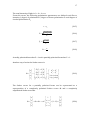
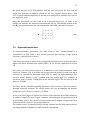
In the rear panel (figure 3.2) there are both a USB connector and a SMA connector
in order to control the laser from a computer and to monitor the pulses produced
by the master source. Also, there is a power connector to supply energy to the laser
and an interlock connector for safety purposes.
The master source is switched on by pressing a button but the laser emission does
not begin until the amplifier is enabled with the key switch.
26
Every time the laser is connected it takes around ten minutes until it reaches the
optimal temperature to work.
Figure 3.2: supercontinuum laser rear panel [21].
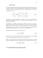
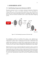
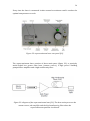
The supercontinuum laser consists of three main parts (figure 3.3): a passively
mode-locked low power fiber laser (master source), a high power cladding
pumped fiber amplifier and a high nonlinearity fiber.
Figure 3.3: diagram of the supercontinuum laser [21]. The three main parts are the
master source, the amplifier and the high nonlinearity fiber where the
supercontinuum spectrum is achieved.
27
- Master source: the master source is a passively mode locked fiber laser.
Fiber lasers are lasers in which its gain medium, instead of being a semiconductor,
is a doped fiber. In this case the fiber is doped with Yb. These type of lasers present
quite interesting qualities such as a high gain efficiency that makes them possible
to operate with low pump power.
Another important characteristic is that the gain bandwidth of the doping element
(Yb) is large which allows the generation of ultra short pulses.
With regard to the operating mode, mode locking [22] is a technique to obtain
ultra short pulses in lasers (picoseconds or femtoseconds pulses) introducing a
fixed phase between the longitudinal modes of the laser’s cavity. There are two
types of mode locking: active and passive. In active mode locking the laser
resonator contains an active element or optical modulator whereas in passive
mode locking a nonlinear passive element or saturable absorber is place inside the
resonator cavity. Besides this, passive mode locking allows the generation of
shorter pulses (femtosecond pulses).
The saturable absorber is a material with a degree of absorption which is
decreases at high optical intensities. It modulates the resonator loses.
- Power amplifier: the high power fiber amplifier is based on a doble-clad
Yb-dopped fiber, pumped by a high power diode. The power is controller manually
by turning the knob in the panel or with the computer.
- Supercontinuum generator: the supercontinuum generator consists of a
length of highly-nonlinear optical fiber, with dispersion and length tailored to
optimize the broadening. In this part is where the broad spectrum is achieved.
3.3. Final setup
In order to select a wavelength to perform the measurement of the Mueller matrix
it is necessary to develop a monochromator since the laser source provides a
continuum spectrum.
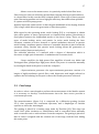
The monochromator (figure 3.4) is composed by a diffraction grating (section
2.5.1), that separates the continuum spectrum, and a diaphragm of variable
aperture to select the wavelength.
The grating is placed in a rotating stage made by Thorlabs [23]. This stage can
rotate 360º either clockwise or anticlockwise and is controlled either manually
with a controller unit or with software from the computer. The grating is placed so
that its center is aligned with the rotation axis of the stage, with the laser hitting
this same point.
28
In addition, the stage is placed on another set of platforms which allows us to
modify the height and the angles in the horizontal and vertical direction.
The manual movement of the stage is carried through a controller unit (TDC001
DC Servo Motor Drive [24]) which allows rotating the stage a certain angle in a
continuous mode or step by step, fixing the step value with the computer.
The software provides information about the position and allows a more accurate
control introducing the value of the position you want (in degrees) directly in the
display. [The display shows the position of the stage with an accuracy of 4
decimals]. Moreover, we can program a series of movements.
Also, it allows changing the value of the step, the movement mode (continuous or
step by step) and the value of the speed rotation.
The laser illuminates the diffraction grating with an incident angle of θi = 31,4º so
that the continuous spectrum is expanded, i.e. it is separated by allowing us to
select a quasi-monochromatic range. Roughly speaking, the continuous spectrum is
separated in the different colors. After the grating, located at 40 cm, it is placed a
diaphragm of variable aperture which select the wavelength interval. This
illuminating setup is aligned with the rest of the polarimeter; therefore, the light
follows the same path as it did with the He-Ne laser source used before.
Figure 3.4: monochromator setup (top view). After the monochromator
characterization the auxiliary setup is removed so the light passes through the
polarimeter.
29
In order to control the reflected beam in the diffraction grating, i.e. the zero order,
a mirror reflects it downwards to a metallic plate located in the table. (It is very
important to absorb this beam because it is very energetic in the infrared region
and it could burn cables, furniture or clothes placed in its way).
All elements that form the monochromator must be perfectly aligned with the rest
of the elements of the polarimeter in order to allow the portion of spectrum
selected by the diaphragm to travel through to travel through the whole
polarimeter and to reach the detector finally.
Not only is this a non-trivial step, but it is a very important one, because it is
necessary to follow a series of instructions in order to be sure that the light will
follow the correct path.
First of all, every element of the experimental setup must be at the same height.
We take as a reference the elements from the PSG and the PSA since they are
already aligned from the previous setup.
Therefore, we must assure that each new element added to the setup (laser source,
grating, diaphragm...) are at the same height.
Then all the elements, except for the source, are placed along the same line. This
line is defined by the elements of the polarimeter and is parallel to the plane of the
table.
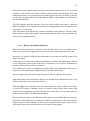
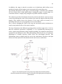
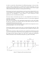
In conclusion, the beam of light must follow the straight line formed by four main
points: the incident point in the surface of the grating, the hole in the diaphragm,
the sample and the detector (figure 3.5). This can be achieved by moving the
different elements in the x direction (In the plane xy or plane of the table).
Figure 3.5: diagram of the experimental setup.
30
Concerning the diffraction grating, its surface normal must be parallel to the plane
of the table. Otherwise, the diffracted beams would deviate from its path. This can
be achieved by moving the platform which allows changing the inclination of the
grating.
The final check of the alignment has been made using as a reference a point in the
wall (distant > 5 m) used to align the original He-Ne laser.
Finally, an important aspect to consider is that the rotating stage can be rotated in
both directions but the last movement must be always clockwise in order to keep
the grating correctly aligned with the rest of the setup.
31
4. RESULTS
4.1. Monochromator characterization
In order to build a monochromator that may be useful in future measurements, an
essential step is to fully characterize it. This means to study the wavelength
selection for different diaphragm apertures and positions of the diffraction grating.
Also, we study the reproducibility of the measures, this is, once we have the curve
of selected wavelength as a function of the position/angle of the rotating stage, we
do several trials moving the stage to a position and checking if the selected
wavelength is the same given by the fitting.
In order to do that, we assemble an auxiliary setup (figure 3.4) in which a mirror
diverts the light beam selected by the diaphragm. This beam is focused onto an
optical fiber by a biconvex lens of focal 150 mm. The spectrum collected by the
fiber is measured by a spectrometer.
4.1.1. Spectrometer calibration
In order to control the wavelength selected by the monochromator implemented
after the supercontinuum laser, we are going to use a spectrometer. This device
will tell us the interval of wavelengths we are selecting from the continuum
spectrum.
But, first of all, we need to study the response of the device. This will allow us to
know the resolution with which we can measure the wavelength.
We are going to use the spectrometer USB2000 [24], from Ocean Optics, Inc. (The
spectrometer is powered by a computer through an USB). An optical fiber is
attached to the device in order to collect the light from a source. The program
reads the counts at several wavelengths and saves this information in a text file
which can be imported to a plotting program in order to represent the spectrum
graphically.
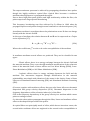
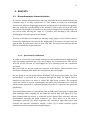
This small spectrometer is a closed box with an USB port for the power supply and
data exchange, and a coupling for the input the optical fiber (See figure 4.1). The
light coming from the source is collected by the optical fiber and goes into the
spectrometer through the SMA connector (1). Then, there is a slit with a
rectangular aperture (2), which regulates the amount of light that enters and
controls the spectral resolution. Finally, a filter (3) is found restricts optical
radiation to pre-determined wavelength regions.
32
Inside the device, the light encounters a collimating mirror (4) which focuses the
light towards a diffraction grating (5). This grating diffracts the light and guides it
to a second mirror (6) which focuses the light onto the detector (8).
This detector, depending on the spectrometer configuration, is a CCD detector or a
L2 Detector Collection Lens (9). The last one is used when there is a low light level.
Figure 4.1: spectrometer USB2000 [25]. (1): SMA connector; (2): slit; (3):
filter; (4): collimating mirror; (5): diffraction grating; (6): mirror; (7 y (8):
detector.
In order to know the resolution achieved by the spectrometer we measured the
spectrum of an He-Ne laser since it is formed by a single well-known wavelength of
λHe-Ne = 6328 Å. First of all, we measure the spectrum of the backlight, with the
laser off. Then, we measure the spectrum with the laser on. The software allow us
to measure the counts at each wavelength in a fixed range, adjusting the
integration time in order to have enough signal but not to saturate the detector.
The backlight spectrum has been subtracted to the measure done with the laser on
in order to obtain the spectrum of the laser. The result is presented in figure 4.2.
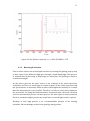
In the spectrum is observed the peak corresponding to the emission of the laser. Its
maximum is at a wavelength λexp = 6330 Å with a Full Width at Half Maximum of
FWHM = 1,5 nm = 15 Å.
Comparing the theoretical value and the experimental result, we find a difference
of 0,2 nm and a width of 1,5 nm. These will be the precision and resolution values
with which we will characterize our instrument, more then enough for our
purposes.
33
Figure 4.2: He-Ne laser spectrum. λexp = 6330 Å, FWHM = 15 Å.
4.1.2. Wavelength selection
First of all we achieve the wavelength selection by rotating the grating step by step
so that a part of the diffracted light goes through a small diaphragm. This process
is characterized by knowing in what angle we must place the grating to obtain a
certain wavelength.
As the power given by the laser source is not constant in the entire spectrum,
sometimes we have too much light in certain regions of the visible spectrum and
the spectrometer is saturated, while in other wavelengths the intensity is so small
that the measurement is not possible. Therefore, in order to solve this problem as
far as possible, for doing the monochromator characterization, the laser will work
at low to intermediate powers. At these powers, the blue region is barely achieved
but if we worked at higher powers we would have too much light in other regions.
Working at such high powers is no recommendable because of the heating
problems, like the damage caused in the grating, among others.
34
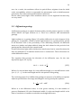
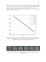
Figure 4.3 shows four measurements made in different days by moving the stage in
0.5º steps. The angle α corresponds to the position of the stage (not the incident
angle) and λ is the maximum wavelength measured with the spectrometer.
Experimental data can be approximated by a straight line: λ = m1α + b1. The fitting
results are shown in table 4.1.
Figure 4.3: wavelength λ as a function of the position of the stage α for four different
measurements. The different markers show the experimental points measured. The
continuous lines show the best fitting to a straight line.
1
2
3
4
Mean
m1 / nm/º -14,76±0,08 -14,68±0,06 -14,72±0,08 -14,67± ,11 14,71±0,02
2204±13
b1 / nm
2210±8
2204±6
2208±9
2206±2
R
0,99967
0,9998
0,99956
0,99957
Table 4.1: fitting parameters. m1 is the slope, b1 is the intercept and R is the lineal
correlation index.
35
So, from figure 4.3 and table 4.1, we can see that the experimental points fit almost
perfect to a straight line of slope <m1> = (14,71 ± 0,02) nm/º.
y  14,71x  2206
(4.1)
This fitting will be used to know the wavelength at a certain position of the grating.
These set of measurements has been done by returning the stage to the initial or
zero position manually. This implies a little initial error so it is very hard to place
the stage always in the exactly same initial position. However, we see that the
fitting are very similar for the three sets of values, therefore, returning the stage to
zero manually does not introduce important errors.
It is worth to emphasize that this result is an approximation since the error in the
wavelength at a certain angle α may change depending on the accuracy with which
the stage is placed at cero initially.
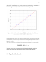
4.1.3. Diaphragm aperture
To complete the monochromator characterization we measure the full width at
half maximum (FWHM) of the spectrum selected by the diaphragm with different
apertures.
The aperture ϕ varies from 1 mm to 3 mm in steps of 0,2 mm and the laser works
at a power of Q = 700. Figure 4.3 shows the variation of the FWHM when the
aperture increases. The measures have been done at a wavelength of λ = 519,1 nm.
As it was expected the FWHM increases linearly with the size of the aperture
(figure 4.4). At first sight, it can be thought that the straight line must pass through
the origin (0, 0). However, this is not true since the smallest FWMH, this is, the
intercept in figure 4.4 is given by the smallest resolvable wavelength difference
(∆λ)min (equation 2.31).
From this equation we calculate (∆λ)min [Wg ≈ 1.5 mm at 530 nm, m = 1, λ = 519,1
nm and k = 1800 g/mm].
R = 2700  (∆λ)min ≈ 0,2 nm
Comparing the result above with the intercept to the figure, b2 = (0,4 ± 0,1) nm we
see that both are coherent although the results are slightly different. This can be
because theoretical calculation is an approximation since we don’t really know the
36
value of the beam diameter at a certain power and wavelength so the number of
illuminated grooves may be smaller and so the resolution power R.
Figure 4.4: full width at half maximum (FWHM) as a function of the diaphragm
aperture ϕ. m2 = (1,03 ± 0,05), b2 = (0,4 ± 0,1)nm.
Another interesting aspect that attracts attention from figure above is that the
spectral width increases in steps and therefore making the experimental points to
appear in couples.
This effect is due to the resolution of the spectrometer that can be assessed to be:
(3, 6  1, 4)nm 2, 2

 0,37 nm
6
6
Therefore, we can’t see a variation in the FWHM smaller than this resolution
Despite this fact, it is still appreciable the linear behavior of the figure 4.4.
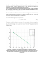
4.2. Reproducibility of results
37
In order to perform the alignment of the laser and the monochromator with the
rest of the setup (sample + detection area), it was necessary to change the
inclination of the diffraction grating and not only its height.
Then, we decided to repeat the measurements done in section 4.2.1. We found that
the slope of the straight line in figure 4.3 changed, thought only slightly. In figure
4.5 and table 4.2 we can see the final result.
We have made three different measures of the wavelength as a function of the
stage position, varying the position of the stage one degree per step. As we did
before, the data has been adjusted to a straight line.
So, the final fitting is given by the expression:
y  14,89 x  2194
(4.2)
Finally, we decided to check the accuracy of the wavelength selection system that
we have characterized. To do that, we took several measurements different
positions of the stage and compare the results with the fitting given by the
equation (4.2).
Figure 4.5: wavelength λ as a function of the position α of the stage α for three
different measurements after completing the alignment. The different markers show
the experimental points measured. The continuous lines show the best fitting to a
straight line.
38
1
2
3
Mean
m1 / nm/º -14,91±0,09 -14,9±0,1 -14,87±0,1 14,89±0,01
b1 / nm
2196±9
2196±11 2191±10
2194±2
R
0,99975
0,99981
0,99976
Table 4.2: fitting parameters. m1 is the slope, b1 is the intercept and R is the lineal
correlation index.
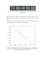
Figure 4.6 shows the straight line obtained from the fitting in table 4.2. This line
will tell us what wavelength we are measuring when the stage is placed at a certain
angle α.
This figure also shows seven experimental points, in blue. The differences between
experimental points and the fitting are shown in table 4.3.
Figure 4.6: final fitting that shows the selected wavelength λ at a certain position of
the stage α. The markers show some experimental points. The continuous line is
obtained from the measures in figure 4.5
39
α / º λexp / nm
100,3 700,66
102,5 669,94
105
632,99
106,5 610,51
108
588,89
110,2 554,75
111,5 533,80
λfit / nm
700,54
668,14
631,02
609,73
586,14
552,43
534,19
|∆λ| / nm
0,12
1,8
1,97
0,78
2,75
2,32
0,39
Table 4.3: position of the stage (α), selected wavelength predicted by the fitting (λfit),
experimental wavelength measured (λexp) and difference between both of them.
From table 4.3 we see that the differences are less than 3 nanometers, being the
average deviation smaller than 2 nm. This is an acceptable error.
4.3. DRCP calibration at different wavelengths
Finally, in order to check that the new source implemented works fine in the DRCP,
we have performed some calibration cycles at different wavelengths and we have
obtained their Mueller matrices. Ideally, the calibration matrix has to be the
identity matrix (equation 3.1).
The measurements have been done with a diaphragm aperture of approx. 1 mm
for six positions of the stage at 104, 106, 108, 110, 112 and 114º, which
correspond, according to figure 4.6, with the central wavelengths: λ1 = 645 nm , λ2
= 616 nm, λ3 = 586 nm, λ4 = 556 nm, λ5 = 526 nm and λ6 = 497 nm . Intensity
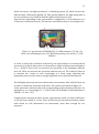
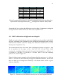
patterns are shown in figure 4.7.
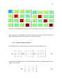
Figure 4.8 shows some examples of the calibration Mueller matrices at λ2 = 616 nm
and λ4 = 556 nm. We have achieved pretty good calibration matrices, but the fact
that we didn’t get a homogeneous intensity of the beam makes harder to get a
uniform calibration.
Figure 4.7: elements m00 of the Mueller matrix for the six wavelengths measured.
40
Figure 4.8: calibration Mueller matrices at wavelengths λ2 = 616 nm and λ4 = 556 nm.
After doing these calibrations, we have studied some optical elements. We have
done and spectral study of the behavior of a linear polarizer.
4.3.1. Study of a linear polarizer
The Muller matrices of an ideal linear polarizer at 0º, 90º and ±45º are:
1
1
M0  
0

0
1 0 0
 1 1

 1 1
1 0 0
M 90  
0 0
0 0 0


0 0 0
0 0
0 0
1

0
0 0
M 45  
 1
0 0


0 0
0
0 1 0 
0 0 0 
0 1 0

0 0 0
(4.3)
In general, the Mueller matrix of a linear polarizer with its transmission axis in an
angle α would be [8]:
 1
c
M   2
 s2

 0
c2
c22
s2
s2 c2
s2 c2
0
s22
0
0
0 
0

0
(4.4)
41
Where c2α = cos (2α) and s2α = sin (2α).
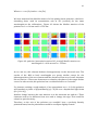
We have measured the Mueller matrix of a low-quality linear polarizer, a dichroicabsorbing sheet, with its transmission axis at 90º (vertical) for the same
wavelengths as the calibrations. Figure 4.9 shows the Mueller matrices of the
polarizer at λ2 = 616 nm and λ4 = 556 nm.
Figure 4.9: polarizer (transmission axis at 90º, vertical) Mueller matrices at
wavelengths λ2 = 616 nm and λ4 = 556 nm.
As we can see, this element behaves homogeneously in the observed area. The
results of the MM at both wavelengths are pretty similar except for the
inhomogeneities of the m00 element and the deviation from zero of some elements
like m30 and m31. These two elements are related to the phase of the output Stokes
vector. In other words, this polarizer has a residual behavior as “retarder”.
For instance, making a rough analysis, if we approximate m30 ≈ -0.3, this polarizer
will introduce a phase of approximately |φ| ≈ π/20 over a depolarized light beam
(S = [1 0 0 0]’).
Another change between the two matrices is in the elements m20 and m21. These
elements seem to be different from zero and to change the sign. This would be
related to optical activity.
Therefore, at the exit of the polarizer we wouldn’t’ have a perfectly linearly
polarized beam, but the polarization would be an ellipse slightly rotated.
42
5. CONCLUSIONS AND FINAL REMARKS
The main goal of this project has been to improve the Dual Rotating Compensator
Polarimeter (DRPC) placed at the Optics laboratory by replacing a He-Ne laser by a
supercontinuum laser source. This laser provides a wide spectrum that can be
used to perform measures of the Mueller Matrix at any desired wavelengths in the
visible region.
In order to do that, several tasks have been carried out:
 Study of the basic theory about polarimetry: applications, Jones and Stokes
Muller formalism, polarimeters…
 Handling the DRCP in the laboratory. This step implies learning how it
works and how to perform a measure of the Mueller Matrix.
 The next step was learning how to operate the different parts of what it was
going to be the source and monochromator: supercontinuum laser, rotating
stage, diffraction grating…
 Then, all the elements were assembled and the monochromator was built,
replacing the previous source (He-Ne laser) by the new setup.
 Once all the elements were in the correct place, the monochromator was
characterized by means of an auxiliary setup shown in figure 3.3. We have
measured the wavelength selected by the diaphragm as a function of the
position of the stage (figure 4.5) and we have studied the spectral width of
the transmitted light as a function of the diaphragm aperture (figure 4.4).
 After the characterization the whole set up was correctly aligned with the
rest of the DRPC so that the light follows the appropriate path reaching the
sample and the detector.
 Finally, the correct working of the whole set up was checked by obtaining
some calibrations Mueller matrix at different wavelengths (figure 4.8).
 Also, we have done a spectral study of a linear polarizer. We have measured
its Mueller matrix with its transmission axis at 90º at different wavelengths
(figure 4.9).
43
Regarding future work, and concerning the proper working of the
spectropolarimeter, it would be important trying to achieve a more homogeneous
and constant intensity of the beam in order to obtain a better calibration matrix.
(As we can see in figure 4.7, the intensity distribution in elements m00 is quite
inhomogeneous. The same happens in the Mueller matrices of the polarizer).
Of course, now that we are able to perform measures at any desired wavelength in
the visible region, it would be very interesting to study samples or system whose
Mueller matrices may present a variation along the visible spectrum.
Ideally, a living tissue containing some kind of immersed inhomogeneity would
reveal the capabilities of this system to identify and locate the embedded object. In
practical terms, other dense media with some wavelength-selective embedded
object could be devised, so that a systematic study could be accomplished.
44
6. BIBLIOGRAPHY
[1] Michael F. Sterzik, Stefano Bagnulo2 & Enric Palle. “Biosignatures as revealed by
spectropolarimetry of Earthshine”. Nature, Vol. 483, 64-66, March 2012.
[2] H. Canovas, S.V. JeffersEFFERS, M. De Juan Ovelar, M. Rodenhuis & C.U. Keller.
“ In search of biosignatures.” Nature, Vol. 483, 64-66, March 2012.
[3] James Hough. “Polarimetry: a powerful diagnostic tool in astronomy”. A&G, Vol.
47, June 2006.
[4] J. Scott Tyo, Dennis L. Goldstein. “Review of passive imaging polarimetry for
remote sensing applications”. Applied Optics, Vol. 45, Nº 22, August 2006.
[5] Triple enlace. Polarimetría (II): Aplicaciones en Química.
http://triplenlace.com/2012/11/25/polarimetria-ii-aplicaciones-en-quimica/
[6] Nirmalya Ghosh and I. Alex Vitkin. “Tissue polarimetry: concepts, challenges,
applications, and outlook”. Journal of Biomedics Opticss, Vol. 16(11), November
2011.
[7] Andreas H. Hielscher, Angelia A. Eick. “Diffuse backscattering Mueller matrices
of highly scattering media”. Optics Express, Vol. 1, Nº 13.
[8] Juan Marcos Sanz Casado. “Polarimetría de sistemas difusores con
microestructuras: efectos de difusión múltiple”. Julio 2010.
[9] J. M. Sanz,* C. Extremiana, and J. M. Saiz. “Comprehensive polarimetric analysis of
Spectralon white reflectance standard in a wide visible range”. Applied Optics.
Vol. 52, Nº 24, August 2013.
[10] Francesco Carmagnola, J.M Sanz and J.M Saiz. “Development of a Mueller matrix
imaging system for detecting objects embedded in turbid media”
[11] Craig F. Borhen. “Absorption and Scattering light by small particles. Chapter 2:
electromagnetic theory”. John Wiley & Sons, 1998.
[12] J.J. Gil. “Polarimetric characterization of light and media”. Eur. Phys. J. Appl.
Phys. 40, 1–47 (2007).
[13] Toralf Scharf. “Polarized Liquid Crystals and Polymers”. Chapter 1: polarized
light. John Wiley & Sons, 2007
45
[14] Russell A . Chipman. “Handbook of Optics. Chapter 22: Polarimetry”. McGraw Hill, 2009.
[15] Shih-Yau Lu and Russell A. Chipman. “Interpretation of Mueller matrices
based on polar decomposition.” J. Opt. Soc. Am. A/Vol. 13, No. 5/May 1996
[16] R. R. Alfano* and S. L. Shapiro. “Observation of Self-Phase Modulation ans
Small-Scale filaments in crystal and glasses”. Physical Review Letters, Vol. 24,
Nº 11, March 1970.
[17] Govind P. Agrawal. “Nonlinear fiber optics”. San Diego: Academic Press, 2001.
[18] Christopher Palmer and Erwin Loewen. “Diffraction grating handbook.
Chapter 2: the physics of diffraction gratings”. Newport Corporation, 2005
[19] Diffraction grating GR13-1850 (Grating specifications). Thorlabs.
http://www.thorlabs.com/thorcat/11700/GR13-1850-SpecSheet.pdf
[20] R.M.A. Azzam. “Photopolarimetric measurement of the Mueller matrix
by Fourier analysis of a single detected signal”. Optical Letters, Vol. 2, Nº 6. June
1978.
[21] Femto Power 1060 Super Continuum Laser Source User’s manual.
[22] Rüdiger Paschotta. RP Photonic Encyclopedia (Mode Locking)
http://www.rp-photonics.com/mode_locking.html.
[23] CR1-Z7, CR1/M-Z7 Motorized Rotation Stage Operating Manual. Thorlabs
http://www.thorlabs.com/thorcat/17000/CR1-Z7-Manual.pdf
[24] TDC001 DC Servo Motor Driver User’s Guide. Thorlabs.
[25] USB2000 Fiber Optic Spectrometer Operating Instructions. Ocean Optics.
46
47
BLOCK II
1. INTRODUCTION
Last year I was awarded a scholarship under the agreement between the
University of Cantabria and the University of Brown (Providence, RI, USA).
From June 16th to August 8th, I stayed in the School of Engineering under the
supervision of Prof. R. Zia [1].
This group works mainly in the fields of nanophotonics, materials science, optical
physics, and physical chemistry. Specifically, they study the multipolar transitions
and how light is emitted from solid-state quantum emitters (like atoms, defect
centers, ions, molecules, and quantum dots).
They investigate new ways to control and enhance the process of light emission for
photonic devices by developing new techniques to directly quantify and access
specific transitions.
This research group receives students from the fields of physics and engineering. It
is currently formed by four Ph.D. students and several undergrad students; all of
them coordinated by Prof. Rashid Zia, the head of the group.
During my stay there, I have participated in the daily life and routines of the group,
I attended several training courses and I have been assigned different tasks like
preparing and attending oral presentations, helping other students at the lab or
learning some specific concepts.
48
2. TASKS
2.1 Daily life
The first task I was assigned was to prepare an oral presentation, in order to show
the rest of the group my work done back in Spain.
In the same way, during the weeks, I attended presentations prepared by the rest
of the undergrad students, where they explained the work they were carrying out
during the summer.
This included topics such as optical activity and chiral molecules, molecular scale
imaging techniques or thermodynamics.
On the other hand, I attended the presentation of the PhD work of one of the
students, a research about wide-angle energy-momentum spectroscopy [2].
This technique allows the simultaneous measurement of the momentum and
spectral distribution of light emission and can reveal a lot of information about the
electronic structure of the emitter.
He studies the emission rates for magnetic and electric dipole transitions in
europium-doped yttrium oxide (Eu3+:Y2O3) and chromium-doped magnesium
oxide (Cr3+:MgO). In order to do that, he images the back focal plane of a
microscope objective to obtain the radiation pattern and project it onto two
orthogonal polarizations with a Wollaston prism. Finally, he disperses them in the
different wavelengths using a diffraction grating.
At the same time, some afternoons, undergrad student went down to the
laboratory and help Ph.D. students and the Professor so that we could learn how to
work in the lab.
For instance, I helped to assemble and align a setup for doing microphotoluminescence-excitation-spectroscopy on very low concentration quantum
emitters. The setup consisted of a white light source, several parabolic mirrors to
guide and focus the light, a diffraction grating to expand the continuous spectrum,
a slit to select a wavelength interval, a sample holder and a spectrometer. This
experimental setup was specially interesting for its proximity with that of my UC
project.
2.2. Compulsory training courses
In order to be allowed to work in the lab, it was necessary to attend several
training courses. These courses were mandatory for all students, research staff, or
49
any person working in the different laboratories at Brown and they covered the
basic knowledge and skills you have to acquire in order to work safely.
In my particular case, I attended three courses which included both classroom and
online classes:
- Laser Safety Training:
It was an online course oriented to revise the main parts of a laser and the basic
concepts and physic behind its working.
Also, it presented the classification of lasers regarding their power and its potential
hazard (classes 1, 1M, 2, 2M, 3R, 3B and 4 from safer to more hazardous).
Of course, the course also explained the potential damages laser can made to eyes
or skin depending on the wavelength, as well as, the security measures you have to
take in order to safely work with the different classes of lasers.
- Hazardous Waste Training:
This course explained how the University of Brown manages (storage, pick-up
routines and transport) wastes, specially hazardous wastes, generated at the labs.
I learnt to identify solid wastes and the regulations that show how they must be
labeled and stored in a proper container depending on its characteristics, as well
as how to proceed in case of an emergency involving hazardous wastes.
- Laboratory Safety Training:
This course covered different topics regarding the general safety in laboratories:
emergency procedures, fire safety, electrical safety, an introduction to Chemical
Hygiene Plan, Material Safety Data Sheets (MSDS), how to work with chemicals,
security measures working on the lab (gloves, glasses, lab coat…), how to manage
compressed gas cylinders, reactive chemical, fume hoods…
2.3. Movement of a rotating stage using Matlab Executable (Mex)
files
Another task was to develop some programs written in C++ code in order to
control the movement of a rotating stage using Mex-files.
We wanted the stage to perform two main movements: a home movement (return
the stage to the origin) and an absolute movement (rotate the stage a certain angle).
50
In order to communicate with the stage we will use the Host-Controller
Communications Protocol given by Thorlabs [3] and the D2XX functions [4]
The stage used is a PRM1Z8 Motorized Rotation Stage controlled by a TDC001 TCube DC Servo Motor Controller, both made by Thorlabs [5].
Mex-files [6], [7] are able to call C or Fortran routine directly from Matlab. Mex
stands for Matlab Executable. This means that you can run a code written in C++
from Matlab as if it were a built-in function. Mex-files can be called exactly like Mfunctions in MATLAB.
In order to write a Mex-file we need to include a gateway routine: mexFunctions.
Matlab uses it as the entry point to the function.
We need to write the following code:
# include “mex.h”
void mexFunction (int nlhs, mxArray *plhs[], int nrhs, const mxArray *prhs[]) {
/* Here we write our C code ... For instance:*/
mexPrintf (“Hello World!”);
}
Where nlhs is the number of output arguments, nrhs is the number of input
arguments and plhs and prhs are arrays with the output and input arguments
respectively.
Inside this gateway routine we can write our function in C code. The header #
include “mex.h” is always necessary.
We save our program whit the extension hello.cpp. The name of the file with the
gateway will be the command name in Matlab. After this, we need to chose a
suitable compiler (write mex –setup in the command window and select the
compiler) and compile it by writing mex hello.cpp. Once the code is compiled we can
call the file from the command window in Matlab as it were a m-file.
For instance, when we type hello in the command window, the code above will
print the words Hello World!
Using the commands described in reference [4] and [5] we were able to
successfully compile the code and to initiate the communications with the stage. I
explained how to use Mex-files to my teammate and he will continue working on
this project.
51
3. BIBLIOGRAPHY
[1] The Zia Lab. http://www.zia-lab.com
[2] Christopher M. Dodson,∗ Jonathan A. Kurvits,∗ Dongfang Li, and Rashid Zia.
School of Engineering and Department of Physics, Brown University,
Providence, RI. “Wide-angle energy-momentum spectroscopy.”
[3] Thorlabs APT Controllers Host-Controller Communications Protocol.
http://www.sal.wisc.edu/manga/archive/public/datasheets/thorlabs/APT_C
ommunications_Protocol_Rev%203.pdf
[4] Software Application Development D2XX Programmer's Guide.
http://www.ftdichip.com/Support/Documents/ProgramGuides/D2XX_
Programmer's_Guide(FT_000071).pdf
[5] PRM1Z8 Motorized Rotation Stage user’s manual.
http://www.thorlabs.com/thorcat/19700/PRM1Z8-Manual.pdf
[6] Maria Axelsson. “An introduction to MATLAB An introduction to MATLAB MEX
Files.” http://pages.cs.wisc.edu/~ferris/cs733/Seminarium_CBA_ht07_
MATLAB_ MEX_ handouts.pdf
[7] http://www.mathworks.es/
52