Download FLO-TOTE 3 Sensor User Manual - English

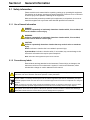
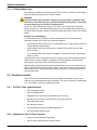
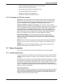
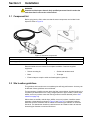
DOC026.53.00787
Flo-Tote 3 Sensor
Open Channel Flow Sensor
User Manual
November 2013, Edition 4
© Hach Company, 2010. All rights reserved. Printed in the U.S.A
jk/kt
Table of Contents
Section 1 Specifications .................................................................................................................... 3
Section 2 General Information ......................................................................................................... 5
2.1 Safety information ........................................................................................................................ 5
2.1.1 Use of hazard information................................................................................................... 5
2.1.2 Precautionary labels ........................................................................................................... 5
2.1.3 Confined space entry .......................................................................................................... 6
2.2 Product overview ......................................................................................................................... 6
2.2.1 Flo-Tote 3 flow system features.......................................................................................... 6
2.2.2 Applications of a Flo-Tote 3 system .................................................................................... 6
2.2.3 Advantages of a Flo-Tote 3 system .................................................................................... 7
2.3 Theory of operation...................................................................................................................... 7
2.3.1 Velocity measurement ........................................................................................................ 7
2.3.2 Depth measurement ........................................................................................................... 8
2.3.3 Flow calculation .................................................................................................................. 8
Section 3 Installation.......................................................................................................................... 9
3.1 Component list ............................................................................................................................. 9
3.2 Site location guidelines ................................................................................................................ 9
3.3 Sensor installation...................................................................................................................... 12
3.3.1 Sensor installation kits ...................................................................................................... 12
3.3.2 Connection to the Flo-Logger, FL900 Series Logger or Flo-Station ................................. 12
3.4 Dams for low-flow applications .................................................................................................. 13
3.4.1 Dam construction .............................................................................................................. 13
3.4.2 Dam installation ................................................................................................................ 14
Section 4 Maintenance .................................................................................................................... 15
4.1 Sensor cleaning ......................................................................................................................... 15
4.2 Changing the Sensor Desiccant ................................................................................................ 15
4.2.1 Desiccant replacement procedure .................................................................................... 15
4.3 Hydrophobic filter description..................................................................................................... 16
4.4 Hydrophobic filter replacement procedure ................................................................................. 17
Section 5 Troubleshooting ............................................................................................................. 19
Section 6 Contact Information ....................................................................................................... 21
Appendix A Velocity profiling ........................................................................................................ 23
A.1
A.2
A.3
A.4
A.5
About velocity profiling............................................................................................................... 23
Site selection ............................................................................................................................. 24
Profile guidelines ....................................................................................................................... 24
Depth of flow measurements..................................................................................................... 24
Velocity profile calculations ....................................................................................................... 25
A.5.1 .9 x Vmax method............................................................................................................. 25
A.5.2 .2, .4, .8 method................................................................................................................ 26
A.5.3 .4 method.......................................................................................................................... 26
A.5.4 2D method ........................................................................................................................ 26
A.6 Auto-Cal automatic calibration................................................................................................... 28
A.7 Calibrate the sensor using the Cal Wizard in the Flo-Ware software ........................................ 28
Appendix B Flow calculations ....................................................................................................... 29
B.1
B.2
B.3
B.4
Circular channels....................................................................................................................... 29
Rectangular channels................................................................................................................ 32
Rivers and streams.................................................................................................................... 33
Flow unit conversions ................................................................................................................ 35
1
Table of Contents
2
Section 1
Specifications
Specifications are subject to change without notice.
Table 1 Sensor specifications
General
Material
Polyurethane
Dimensions
13.1 cm W x 4.4 cm L x 2.8 cm diameter (5.16 in. x 1.73 in. x 1.10 in.)
Weight
1.1 kg (2.4 lb) with 30 ft cable
Operating temperature
0 to 45 °C (32 to 113 °F)
Operating humidity
0-100%
Storage temperature
–20 to 52° C (–4 to 125° F)
Power requirements
10V, 100 mA. Sensor power is supplied by the portable Flo-Logger or by the Flo-Station
Monitor.
Method: Electromagnetic (Faraday’s law)
Range: –1.5 to 6.1 m/s (–5 to 20 ft/s)
Velocity measurement
Accuracy: ± 2% of reading
Zero stability: ± 0.015 m/s (± 0.05 ft/s) at 0 to 3 m/s (0 to 10 ft/s)
Resolution: ± 0.0003 m/s (0.01 ft/s)
Method: Submerged pressure transducer
Range: Standard 10 mm to 3.5 m (0.4 to 138 inches). Contact the factory for extended ranges
Accuracy: ± 1% reading
Depth measurement
Zero stability: ± 0.009 m (± 0.03 feet), for 0 to 3 m (0 to 10 ft)
Includes non-linearity, hysteresis and velocity effects.
Resolution: 2.5 mm (0.1 in.)
Over range protection: 2X range
Flow measurement
Method: Conversion of water level and pipe size to fluid area. Conversion of local velocity
reading to mean velocity. Multiplication of fluid area by mean velocity to equal flow rate.
Conversion accuracy: ± 5.0% of reading. Assumes appropriate site calibration coefficient, pipe
flowing 10% to 90% full with a level greater than 5.08 cm (2 in.).
Method: 1 wire digital thermometer
Temperature
measurement
Range: –10 to 85 °C (14 to 185 °F)
Accuracy: ± 2 °C (± 3.5 °F)
Material: Polyurethane jacketed
Sensor cable
Standard length: 9.1 m (30 ft)
Optional length: 18.2 m, 30.4 m (60,100 ft) or length as needed; maximum 304 m (1000 ft)
Warranty
Warranty
One year from date of shipment. Does not apply to such consumable components, such as,
but not limited to, desiccants and batteries.
3
Specifications
4
Section 2
General Information
2.1 Safety information
Please read this entire manual before unpacking, setting up or operating this equipment.
Pay attention to all danger, warning and caution statements. Failure to do so could result
in serious injury to the operator or damage to the equipment.
Make sure that the protection provided by this equipment is not impaired, do not use or
install this equipment in any manner other than that specified in this manual.
2.1.1 Use of hazard information
DANGER
Indicates a potentially or imminently hazardous situation which, if not avoided, will
result in death or serious injury.
WARNING
Indicates a potentially or imminently hazardous situation which, if not avoided,
could result in death or serious injury.
CAUTION
Indicates a potentially hazardous situation that may result in minor or moderate
injury.
Notice: Indicates a situation that is not related to personal injury.
Important Note: Indicates a situation which, if not avoided, may cause damage to the
instrument. Information that requires special emphasis.
Note: Information that supplements points in the main text.
2.1.2 Precautionary labels
Read all labels and tags attached to the instrument. Personal injury or damage to the
instrument could occur if not observed. A symbol, if noted on the instrument, will be
included with a danger or caution statement in the manual.
This is the safety alert symbol. Obey all safety messages that follow this symbol to avoid potential injury. If on the
instrument, refer to the instruction manual for operation or safety information.
Electrical equipment marked with this symbol may not be disposed of in European public disposal systems after 12
August of 2005. In conformity with European local and national regulations (EU Directive 2002/96/EC), European
electrical equipment users must now return old or end-of life equipment to the Producer for disposal at no charge to
the user.
Note: For return for recycling, please contact the equipment producer or supplier for instructions on how to return
end-of-life equipment, producer-supplied electrical accessories, and all auxiliary items for proper disposal.
This symbol, when noted on the product, indicates the presence of devices sensitive to Electro-static Discharge
(ESD) and indicates that care must be taken to prevent damage with the equipment.
5
General Information
2.1.3 Confined space entry
The following information is provided to guide users of Flo-Tote 3 sensors on the dangers
and risks associated with entry into confined spaces.
WARNING
Potential confined space hazards. Training in pre-entry testing, ventilation, entry
procedures, evacuation/rescue procedures and safety work practices is necessary
to ensure against the loss of life in confined spaces.
On April 15, 1993, OSHA's final ruling on CFR 1910.146, Permit Required Confined
Spaces, became law. This standard directly affects more than 250,000 industrial sites in
the United States and was created to protect the health and safety of workers in confined
spaces.
Definition of Confined Space
A Confined Space is any location or enclosure that presents or has the immediate
potential to present one or more of the following conditions:
•
An atmosphere with less than 19.5% or greater than 23.5% oxygen and/or more than
10 ppm Hydrogen Sulfide (H2S)
•
An atmosphere that may be flammable or explosive due to gases, vapors, mists,
dusts, or fibers
•
Toxic materials which upon contact or inhalation, could result in injury, impairment of
health, or death
Confined spaces are not designed for human occupancy. They have restricted entry and
contain known or potential hazards. Examples of confined spaces include manholes,
stacks, pipes, vats, switch vaults, and other similar locations.
Standard safety procedures must always be followed prior to entry into confined spaces
and/or locations where hazardous gases, vapors, mists, dusts, or fibers may be present.
Before entering any confined space check with your employer for procedures related to
confined space entry.
2.2 Product overview
The Flo-Tote 3 sensor measures the velocity and depth of conductive liquids in open
channels using electromagnetic sensor technology. The sensor connects to a data logger
or to a Flo-Station to make a complete flow system.
2.2.1 Flo-Tote 3 flow system features
•
Fully submersible sensor
•
Debris-shedding sensor
•
Measurement for extremely low velocities and reverse flow
•
Operation under free flow, non-free flow or surcharge conditions
•
Field replaceable sensor
•
No calibration required
•
Increased signal intensity for greasing applications
•
Flow temperature measurement
2.2.2 Applications of a Flo-Tote 3 system
6
•
Perform inflow & infiltration (I&I) studies
•
Perform water distribution/leak isolation studies
General Information
•
Evaluate existing sewer systems and storm water systems
•
Monitor the flow from towns and cities
•
Monitor the sewer overflow into streams and rivers
•
Monitor the industrial flow from factories
•
Measure the efficiency of pump stations
•
Validate the accuracy of existing flow meters
2.2.3 Advantages of a Flo-Tote 3 system
Accurate: Flo-Tote 3 flow system uses the most accurate method of calculating flow,
based on the continuity equation: Flow = Average Velocity x Area. Verification of the
Flo-Tote 3 specifications by an independent flow laboratory assures commitment to
accuracy. Thousands of users worldwide have verified Flo-Tote accuracy.
Portable (FL900 Series Logger or Flo-Logger): The Flo-Logger can be moved to
different sites quickly and easily. This means having the ability to accurately measure flow
at all sites, without having to purchase a flow meter for each location. The Flo-Logger
uses (2) standard, six- volt lantern batteries. Refer to the Flo-Logger User Manual
(DOC026.53.00788). The FL900 Series Flow Logger uses (2) or (4) standard, six-volt
lantern batteries and is also compatible with the long-life alkaline battery (8542900).
Refer to the FL900 Series Flow Logger User Manual (DOC026.97.80015).
Permanent (Flo-Station): The four programmable 4–20 mA outputs provide a
convenient way to transfer real-time flow data to SCADA and other data collection
systems, control systems and display devices. Refer to the Flo-Station User Manual
(DOC026.53.00790).
Reliable: The Flo-Tote 3 Flow System even operates under surcharge conditions. The
Flo-Tote 3 sensor contains no moving parts, which makes it more reliable than other
sensors.
Adaptable: The Flo-Tote 3 Flow System adapts to a wide range of pipe sizes and
shapes, eliminating the need for costly weirs or flumes.
2.3 Theory of operation
The Flo-Tote 3 open channel sensor directly measures water velocity and depth.
2.3.1 Velocity measurement
The sensor makes use of Faraday's Law of electromagnetic induction to measure water
velocity. Faraday's Law states: A conductor, moving through a magnetic field, produces
a voltage.
Because water is a conductor, water moving through a magnetic field produces a voltage.
The magnitude of the voltage is directly proportional to the velocity of the water. The open
channel sensor generates an electromagnetic field, creating a voltage in the water. The
two velocity electrodes along with the ground electrode measure this voltage (refer to
Figure 1). A faster water velocity produces a higher voltage. By accurately measuring this
voltage, the velocity is determined.
Non-Fouling electrodes
The sensor features non-fouling electrodes. These are raised, pointed electrodes which
reduce the amount of grease and debris build-up. When the electrodes become coated,
they no longer measure the water velocity accurately. The non-fouling electrodes are
designed to prevent an accumulation of debris.
7
General Information
Figure 1 Electrodes on Flo-Tote sensor
1
Ground electrode
2
Velocity electrodes
2.3.2 Depth measurement
A pressure transducer is used to measure the depth of the water. The transducer is an
electronic device which uses a thin diaphragm to convert pressure to an electronic signal.
The depth transducer is located inside the sensor. The cross channel (located on the
bottom of the sensor) allows water pressure to reach the transducer, while at the same
time protecting the fragile diaphragm from damage.
An air tube, running through the length of cable from the sensor to the desiccant junction
box, enables the transducer to cancel out the atmospheric pressure in order to measure
the true water pressure. The air tube (called the atmospheric pressure reference or APR
tube) needs to be protected from water, which can damage the transducer.
2.3.3 Flow calculation
The velocity and depth measurements provided by the open channel sensor are used to
calculate flow. Flow (also known as Q, flow rate, or throughput) is the amount of fluid
moving through a channel or pipe in a period of time. For example, if 100 gallons of water
move past the sensor in one minute, the flow is 100 gallons per minute (GPM). Flow
calculations are performed by the flow meter (Flo-Logger, Flo-Station or other flow
meters).
To calculate flow, two things are needed:
•
The cross-sectional area of the channel. Cross-sectional area is found using the
dimensions of the channel and the measured depth.
•
The average velocity. Average velocity is found using the sensed velocity (measured
by the sensor). The default calibration coefficient is often adequate. A site calibration
will verify or improve accuracy. A site calibration determines the velocity profile and
calculates the correct calibration coefficient for the particular application. For more
information on velocity profiling, refer to Appendix A on page 23.
Flow is calculated by using the continuity equation:
Flow = AverageVelocity × Area
Q = V×A
where
Q = Flow
V = AverageVelocity
A = Wetted Area (calculated from depth and the channel geometry)
Data is sent from the Flo-Tote 3 electromagnetic sensor to a Flo-Logger, FL900 Series
Logger or a Flo-Station via a cable. Flow data is transferred from the Flo-logger to a
laptop/desktop/PocketPC computer via communications cable.
8
Section 3
Installation
WARNING
Potential confined space hazards. Only qualified personnel should conduct the
tasks described in this section of the manual.
3.1 Component list
Before going into the field, make sure that all sensor components are included in the
shipment. Refer to Figure 2.
Figure 2 Instrument components
1
Flo-Tote 3 sensor
4
Cable connector or bare wires
2
Carabiner clip
5
Desiccant container
3
Hanging strap
6
Desiccant hub junction box
Determine what tools are needed for complete installation. Customer-supplied
equipment:
•
Sensor mounting kit
•
Socket and ratchet wrench
•
Base
•
Tie wraps
•
Electrical tape to wrap the cable and band together (optional)
3.2 Site location guidelines
The guidelines in this section are not mandatory but will help performance. Accuracy can
be affected if these guidelines are not followed.
For best accuracy, install the sensor where the flow is not turbulent. An ideal location is in
a manhole just downstream from a long, straight channel or pipe. Outfalls, vertical drops,
baffles, curves or junctions cause the velocity profile to become distorted (refer to Site
selection on page 24).
Where there are outfalls, vertical drops, baffles, curves or junctions, install the sensor
upstream or downstream as shown in Figure 3 and Figure 4. For upstream locations,
install the sensor at a distance that is at least five times the pipe diameter or maximum
fluid level. For downstream locations, install the sensor at a distance that is at least ten
times the pipe diameter or maximum fluid level.
9
Installation
Figure 3 Sensor location near an outfall, vertical drop or baffle
1
Acceptable upstream sensor location
5
Distance downstream: 10 x pipe diameter
2
Outfall
6
Vertical drop
3
Distance upstream: 5 x pipe diameter
7
Baffle
4
Acceptable downstream sensor location
10
Installation
Figure 4 Sensor location near a curve, elbow or junction
1
Acceptable upstream sensor location
3
Distance downstream: 10 x pipe diameter
2
Acceptable downstream sensor location
4
Distance upstream: 5 x pipe diameter
11
Installation
3.3 Sensor installation
Sensor installation involves attachment of the sensor to a metal band or plate which is
then installed in a pipe or channel.
3.3.1 Sensor installation kits
Several kits are available for sensor installation to accommodate various pipe sizes and
shapes. Installation instructions are provided with each kit.
•
Spring band—circular metal band that stays in place by spring action against the pipe
walls. Available for pipe diameters of 6 to 19 inches. Instruction sheet:
DOC273.53.80001. Optional Q-Stick for installation without manhole entry. Instruction
sheet: DOC273.53.80005.
•
Scissors-jack band—circular metal band that stays in place when a scissors jack is
tightened. Available for pipe diameters of 16 to 61 inches. Instruction sheet:
DOC273.53.80003.
•
Partial bands—metal band that covers the bottom half of a channel and stays in
place by attachment to the channel wall. Instruction sheet: DOC273.53.80002.
•
Rectangular channel mount—pole with metal plates that stays in place by
attachment to the channel ceiling. Instruction sheet: DOC273.53.80004.
3.3.2 Connection to the Flo-Logger, FL900 Series Logger or Flo-Station
Connect the cable from the sensor to the Flo-Logger, FL900 Series Logger or Flo-Station.
12
•
Flo-Logger and FL900 Series Logger—connect the cable from the sensor to the
Flo-Dar connector on the logger.
•
Flo-Station—connect the cable from the sensor to the correct terminal in the
Flo-Station.
Installation
3.4 Dams for low-flow applications
At least two inches of water is necessary for accurate velocity measurements. If the site
frequently experiences low-flow conditions, use a dam to raise the water level. Locate the
sensor at least one foot in front of the dam.
3.4.1 Dam construction
A low-flow dam can be made as follows:
1. Make a mold for the dam from a section of pipe with the same diameter as the dam
site. Place a board at one end of the pipe, and angle the pipe to approximately 30º
(refer to Figure 5).
2. Pour pre-mixed concrete into the mold. The top of the dam should be 2 inches high.
3. Allow the concrete to fully set.
Figure 5 Low-flow dam construction
1
Board
2
Pre-mix concrete
3
Cut-pipe section
13
Installation
3.4.2 Dam installation
Install the dam at the site, approximately one foot downstream from the sensor. The
easiest way to attach the dam to the pipe or channel is with hydrolytic cement or
waterproof caulking. The dam can also be attached with lead anchors and lag bolts.
Installation options are shown in Figure 6.
Figure 6 Installation options for low-flow dams
1
Low-flow dam
5
Lead anchor
2
Flow sensor
6
Pipe outfall
3
Lag bolt
7
Metal strap
4
Bottom of pipe
8
Metal strap
14
Section 4
Maintenance
WARNING
Potential confined space hazards. Only qualified personnel should conduct the
tasks described in this section of the manual.
4.1 Sensor cleaning
Important Note: Do not use sandpaper to clean the non-fouling electrodes. Sandpaper
can damage the electrodes.
1. To clean the sensor, pour a small amount of liquid detergent cleaner on a soft bristle
brush. Use this brush to clean the electrodes on top of the sensor.
2. Rinse with clean water.
Figure 7 Electrodes on Flo-Tote sensor
1
Ground electrode
2
Velocity electrodes
4.2 Changing the Sensor Desiccant
The desiccant canister contains beads of silica gel which ensure proper operation of the
pressure transducer located in the Tote 3 sensor. When the beads are yellow, they can
absorb moisture from the air. When they are green, they are saturated and cannot absorb
any more moisture from the air, and they must be replaced immediately.
The cable assembly with desiccant hub is compatible with either the Flo-Logger or the
FL900 Loggers. When using this cable assembly with the Flo-Logger, do not disconnect
the desiccant cartridge that is attached to the Flo-Logger itself.
Important Note: When the beads begin to turn green, replace or rejuvenate the beads.
Permanent damage to the sensor may occur if the desiccant is not maintained. Never
operate the sensor without the proper desiccant. When rejuvenating beads, remove them
from the canister and heat at 100-180 ºC (212-350 ºF) until the beads turn yellow. If the
beads do not turn yellow, replace them with new beads. Do not heat the canister.
4.2.1 Desiccant replacement procedure
Note: Replacing the desiccant does not require that the desiccant container be removed from the
desiccant box.
1. Use a slight twisting motion to twist the bottom end-cap until its slots align with the
retaining clips (Figure 8).
2. Gently remove the end cap by grasping it and pulling it straight out.
3. Pour the desiccant beads out of the canister.
4. Hold the canister up to the light and inspect the hydrophobic filter.
•
If you see a small, dim light spot while looking through the hole, the filter is in good
condition. If you see a bright light spot, the filter is probably torn. Replace the filter.
15
Maintenance
•
If the desiccant beads were completely saturated with water or the filter has saturated
with water or grease, replace the filter.
5. Refill the canister tube with yellow desiccant beads (Cat. No. 8755500). Inspect the
O-ring (Cat. No. 5252) on the bottom cap for cracking, pits, or evidence of leakage.
Replace if necessary.
Note: Applying O-ring grease to new or dry O-rings improves the ease of insertion, sealing, and life
span of the O-ring.
6. Make sure that the O-ring is clean and free of dirt or debris before replacing the end
cap.
7. Reinstall the end cap.
Figure 8 Remove the bottom end cap
1
End cap
4
Retaining clips
2
Slots for retaining clips
5
Desiccant container
3
O-ring
4.3 Hydrophobic filter description
A single Teflon® hydrophobic filter (Cat. No. 3390) is installed in the top of the canister to
prevent liquid from entering the vent tube.
16
Maintenance
For best performance and to avoid grease buildup on the filter during submergence or
surcharge conditions, hang the canister vertically so that the end cap points downward
(refer to Figure 8).
Note: The Hydrophobic Filter may need replacement at any time the cartridge is submerged or
exposed to excess moisture. Refer to section 4.4.
4.4 Hydrophobic filter replacement procedure
1. Disconnect the tubing from the top of the desiccant canister.
2. Unscrew the hex-head tubing nipple from the top of the canister and discard the old
filter.
3. Discard any remnants of Teflon tape from the nipple threads. Apply two turns of
Teflon tape (Cat. No. 10854-45) to the threads, pulling the tape into the threads until it
conforms to the shape of the threads.
4. Place a new filter over the hole. Make sure that the smooth side of the filter faces the
inside of the canister.
5. Place the threaded nipple on top of the filter.
6. With slight pressure, press the filter into the hole with the nipple threads and begin
threading the nipple into the hole. The filter will deflect upward and feed completely
into the thread until it disappears. The filter must rotate with the nipple as it is
threaded into the cap. If it does not, it is torn. Start over with a new filter.
7. Inspect the installation. In the upper cap, a small, dim light spot should be visible
when held up to the light. A bright spot indicates a torn filter. Start over with a new
filter.
Figure 9 Replacing the hydrophobic filter
1
Filter, smooth side down
2
Hex-head tubing nipple
3
Finished assembly
17
Maintenance
18
Section 5
Troubleshooting
When a problem occurs, isolate the problem to the sensor, the logger or the interconnect
cable. Some typical problems and solutions are shown in Table 2.
Table 2 Troubleshooting table
Problem
Cause
Solution
Sudden drops in velocity
The velocity electrodes are covered
with debris.
Clean the sensor. Make sure the sensor
is installed correctly.
The velocity electrodes are dry.
Make sure the water level is above the
sensor. If the water level is low,
construct a low-flow dam.
The velocity electrodes are covered
with debris or grease.
Clean the sensor.
Noisy velocity
There may be electrical noise in the
pipe.
Identify and eliminate the source of the
interference (if possible).
Depth measurements are incorrect
or drift
Water is in the APR tube.
Replace the desiccant (or APR filter)
cartridge. If possible, remove the sensor
and allow it to dry.
Depth measurements are incorrect
(stuck at zero or at full scale)
The internal depth transducer may be
damaged.
Contact customer support.
Conductivity lost error message
19
Troubleshooting
20
Section 6
Contact Information
Ordering information for the U.S.A.
By Telephone:
(800) 368-2723
By Fax:
301-874-8459
By Mail:
Hach Company
4539 Metropolitan Court
Frederick, MD 21704-9452, U.S.A
Ordering information by e-mail:
[email protected]
Information Required
•
Hach account number (if available)
•
Billing address
•
Your name and phone number
•
Shipping address
•
Purchase order number
•
Catalog number
•
Brief description or model number
•
Quantity
European Union
Flow-Tronic
Rue J.H. Cool 19a
B-4840 Welkenraedt
Belgium
Tel: + -32-87-899799
Email: [email protected]
www.flow-tronic.com
Outside the U.S.A. and EU
Hach Company maintains a worldwide network of dealers and distributors. To locate the
representative nearest you, send E-mail to [email protected] or visit
www.hachflow.co.
Technical Support
Technical and Customer Service Department personnel are eager to answer questions
about our products and their use. In the U.S.A., call 1-800-368-2723. Outside the U.S.A.
and Europe, send E-mail to [email protected] or call 1-301-874-5599.
Repair Service
Authorization must be obtained from Hach Company before sending any items for repair.
To send the monitor to the factory for repair:
1. Identify the serial number of the sensor.
2. Record the reason for return.
3. Call the Customer Service Department (1-800-368-2723) and get a Service Request
Number (SRN) and shipping label.
4. Use the shipping label provided and ship the equipment in the original packaging if
possible.
Note: Do not ship manuals, computer cables, or other parts with the unit unless they are required for
repair.
21
Contact Information
5. Make sure the equipment is free from foreign debris and is clean and dry before
shipping. Sensors returned without cleaning will be charged a fee.
6. Write the SRN number on the shipping box.
7. Make sure that all return shipments are insured.
8. Address all shipments to:
Hach Company
5600 Lindbergh Drive - North Dock
Loveland, Colorado, 80539-0389 U.S.A.
Attn: SRN#XXX
22
Appendix A Velocity profiling
WARNING
Potential confined space hazards. Only qualified personnel should conduct the
tasks described in this section of the manual.
A.1 About velocity profiling
The sensor measures the water velocity at the bottom of the channel or pipe (called the
sensed velocity). To calculate flow, the user needs to know the average velocity across
the entire channel or pipe cross-section.
The average velocity is different from the sensed velocity because the water moves at
different velocities at different parts of the cross section. The process of correcting the
sensed velocity by measuring the average velocity is called profiling.
Profiling a site involves directly measuring the water velocity at several points across the
pipe cross-section to determine the average velocity. The controller uses this profile
information along with the sensed velocity and depth reported by the flow sensor to
calculate the correct site calibration coefficient for the application.
The sensed velocity and depth should be obtained during or close to the time the velocity
profile was done. The correct site calibration coefficient will allow the average velocity to
be calculated accurately from sensed velocity at all depths.
Note: Because the exact procedure for performing a velocity profile will vary depending on the type
of velocity profiling meter, the information included here is for general purposes. Refer to the user
manual for the velocity profiling meter that is used for specific information.
Figure 10 Typical velocity profile
1
Depth
2
Velocity
23
Velocity profiling
A.2 Site selection
A site which has a typical profile shape will give the most accurate results. For most
cases, sites which may be difficult to profile can be identified by a visual inspection. Use
the following guidelines to select a site:
1. The channel should have as much straight run as possible. Where the length of
straight run is limited, the length upstream from the profile should be twice the
downstream length.
2. The channel should be free of flow disturbances. Look for protruding pipe joints,
sudden changes in diameter, contributing side streams, outgoing side streams, or
obstructions. Clean any rocks, sediment, or other debris that might be on the bottom
of the pipe.
3. The flow should be free of swirls, eddies, vortices, backward flow, or dead zones.
Avoid areas that have visible swirls on the surface.
4. Avoid areas immediately downstream from sharp bends or obstructions.
5. Avoid converging or diverging flow (approach to a flume) and vertical drops.
6. Avoid areas immediately downstream from a sluice gate or where the channel
empties into a body of stationary water.
A.3 Profile guidelines
For best possible results:
1. Measure the horizontal and vertical diameter of the pipe. If there is a difference, then
use the average for the inside diameter of the pipe.
2. Make sure the flow is symmetrical.
3. Measure the depth several times during the procedure.
4. Examine the pipe for rocks, sediment and other debris.
A.4 Depth of flow measurements
To perform a velocity profile, measure the depth of flow in the pipe:
1. Measure the inside diameter of the pipe.
2. Measure the distance from the top of the pipe to the top of the water (Figure 11).
3. Subtract this distance from the inside diameter of the pipe. This is the depth of flow.
Note: The depth and velocities must be measured in the same vertical plane (Figure 12).
24
Velocity profiling
Figure 11 Depth of flow measurement
Figure 12 Depth of flow and velocity profile—single plane
A.5 Velocity profile calculations
There are four methods for profiling a site. The method chosen depends on the
conditions at the site.
A.5.1 .9 x Vmax method
The .9 x Vmax method is the simplest method. Measure the velocity at different points of
the cross section to determine the maximum velocity in the pipe. The average velocity is
calculated by multiplying the maximum velocity by 0.9. This method should be used for:
•
Low flows—flows of less than two inches depth.
•
Rapidly changing flows—a flow that is changing more than 10% in three
minutes or less can be classified as rapidly changing.
To profile the flow:
1. Measure the velocity at a series of points throughout the entire flow.
2. Identify the fastest velocity. In most cases, this is located in the center just beneath
the surface.
3. Multiply the fastest velocity by 0.9.
25
Velocity profiling
A.5.2 .2, .4, .8 method
The .2, .4, .8 method is the most common method for profiling a typical flow. The velocity
is measured at three points: .2, .4, and .8 times the total depth of flow. The velocity from
each point is entered into the meter. This method should be used for:
•
Typical flows—any site which does not have any disturbances, obstructions,
turbulence, etc. Refer to Site selection on page 24.
To profile the flow:
1. Measure the depth of flow (refer to section A.4 on page 24).
2. Calculate the measurement positions on the center line:
•
.2 position = 0.2 x depth of flow
•
.4 position = 0.4 x depth of flow
•
.8 position = 0.8 x depth of flow
3. Measure the velocities at the .2, .4, and .8 positions (Figure 13).
4. Calculate the average of the .2 and .8 velocities.
5. Calculate the average of the .4 velocity with the .2 and .8 average from step 4.
Figure 13 Measurement positions for .2, .4, and .8 method
A.5.3 .4 method
The .4 method is a simplified version of the .2, .4, .8 method. The velocity is measured at
the .4 position only. Use this method for:
•
Low flows—sites free of obstructions, etc., but without sufficient depth to
measure the velocity at three points.
A.5.4 2D method
The 2D method uses the velocities from the center line, the vertical velocity lines, and
corners of the flow. Use this method for:
26
•
Asymmetrical flows—sites that have velocities that differ by more than 30% on
either side of the pipe (for example, near a bend).
•
Vertical drops—sites that are near an outfall or other change in depth.
•
Irregular flows—any site thought to have an irregular or non-typical profile.
Velocity profiling
To profile the flow:
1. Find the center line of the flow.
2. Find vertical velocity lines (V V L) that are halfway between the center line and the
side walls of the pipe (refer to Figure 14). Use the widest part of the flow.
3. Measure the velocity at a minimum of 7 different depths along the center line.
4. Measure the velocity along the V V L at different depths. The distance between these
depths should be the same as those on the center line.
5. Measure the velocity at the right and left corners of the flow.
6. Examine the data for any outliers. An outlier will fall outside of the best fit curve
region if a graph were made of the velocity profile.
7. Calculate the average velocity (except outliers) of all measurements (except outliers).
Remember to include the corner measurements.
Figure 14 Velocity profiling for the 2D method
Alternate 2D method
A portable velocity sensor can be used to make a 2D profile. Move the sensor in a swirl
pattern across the entire cross-section (refer to Figure 15). Set the instrument to calculate
the average of these velocity measurements. Refer to the user manual for the portable
velocity sensor for detailed instructions.
Typical procedure (for the Flo-Mate velocity profiling meter):
1. Set the FPA time to the appropriate number of seconds.
2. Place the sensor at the start position and wait for a few seconds.
3. Press <ON/C> and start moving the sensor.
27
Velocity profiling
Figure 15 Velocity measured in a swirl pattern
1
Start position
2
Stop position
A.6 Auto-Cal automatic calibration
For sites with straight-run, circular concrete pipes, an Auto-Cal automatic site calibration
can be used in place of velocity profiling.
A.7 Calibrate the sensor using the Cal Wizard in the Flo-Ware software
Prerequisite:
The sensor must be installed in the process and must be online in order to perform the
calibration. The sensor can be configured and calibrated with the calibration wizard as
follows:
1. In the Flo-Ware software, click on the Programming tab in the FL900 Series Driver
window.
2. Click the Sensor Port [1] (sensor name).
3. Click the CAL WIZARD button. The Calibration Wizard window opens.
4. Selec the options on each screen. When the Calibration Complete screen appears,
click FINISH.
5. Click WRITE TO LOGGER to save the settings.
28
Appendix B Flow calculations
WARNING
Potential confined space hazards. Only qualified personnel should conduct the
tasks described in this section of the manual.
For most applications, the flow in a channel is calculated and recorded by a flow meter.
This appendix is included to calculate the flow manually, or to understand how flow is
calculated.
Flow calculations are provided for:
•
Circular channels (section B.1)
•
Rectangular channels (section B.2 on page 32)
•
Rivers and streams (section B.3 on page 33)
B.1 Circular channels
The following values are necessary before the flow can be calculated:
•
The average velocity in ft/sec (Appendix A on page 23)
•
The depth of flow in inches (in.) at the time of the velocity profile (section A.4 on
page 24)
•
The inside diameter of the channel in inches (in.)
1. Calculate the depth to diameter ratio (L/D) where:
•
L is the depth of flow in inches at the time of the profile.
•
D is the inside diameter in inches.
2. Find the flow unit multiplier (K) from Table 3 on page 30:
a. In the left column, find the L/D ratio from step 1.
b. Move to the right (to the desired units column) to get the flow unit multiplier (K).
Note: Table 3 is for circular conduits only, measured in feet. The multiplier was derived using a
one foot per second flow in a one foot diameter conduit as the model.
3. Convert the diameter to square feet:
•
D2 = (channel diameter in inches ÷ 12) x (channel diameter in inches ÷ 12).
4. Calculate the flow:
•
Flow = K x D2 x average velocity.
Example: What is the flow in millions of gallons per day (MGD) in a 10-inch diameter
channel with a 6-inch depth? The average velocity was found to be 1.5 ft/sec.
L/D = 6 inches/10 inches = 0.6
K = 0.3180
D2 = (10 in ÷ 12)2 = (0.833 ft)2 = 0.694 ft2
Flow = K x D2 x average velocity = 0.3180 x 0.694 ft2 x 1.5 ft/sec = 0.331 MGD
29
Flow calculations
Table 3 Flow unit multiplier
30
L/D
MGD
GPM
CFS
CMM
CMD
LPM
.01
.0009
.5966
.0013
.0023
3.2522
2.2585
.02
.0024
1.6824
.0037
.0063
9.1709
6.3687
.03
.0044
3.0814
.0069
.0117
16.7986
11.6644
.04
.0068
4.7296
.0105
.0179
25.7811
17.9036
.05
.0095
6.5894
.0147
.0249
35.9190
24.9438
.06
.0124
8.6351
.0192
.0327
47.0701
32.6876
.07
.0156
10.8475
.0242
.0411
59.1295
41.0621
.08
.0190
13.2113
.0294
.0500
72.0148
50.0103
.09
.0226
15.7143
.0350
.0595
85.6585
59.4851
.10
.0264
18.3460
.0409
.0694
100.0039
69.4471
.11
.0304
21.0975
.0470
.0799
115.0022
79.8627
.12
.0345
23.9609
.0534
.0907
130.6108
90.7020
.13
.0388
26.9294
.0600
.1019
146.7919
101.9388
.14
.0432
29.9967
.0668
.1135
163.5116
113.5497
.15
.0477
33.1571
.0739
.1255
180.7393
125.5134
.16
.0524
36.4056
.0811
.1378
198.4467
137.8102
.17
.0572
39.7374
.0885
.1504
216.6081
150.4223
.18
.0621
43.1480
.0961
.1633
235.1995
163.3330
.19
.0672
46.6334
.1039
.1765
254.1985
176.5267
.20
.0723
50.1898
.1118
.1900
273.5844
189.9892
.21
.0775
53.8135
.1199
.2037
293.3373
203.7064
.22
.0828
57.5012
.1281
.2177
313.4387
217.6657
.23
.0882
61.2496
.1365
.2319
333.8710
231.8548
.24
.0937
65.0555
.1449
.2463
354.6172
246.2619
.25
.0992
68.9161
.1535
.2609
375.6613
260.8759
.26
.1049
72.8286
.1623
.2757
396.9880
275.6861
.27
.1106
76.7901
.1711
.2907
418.5825
290.9823
.28
.1163
80.7982
.1800
.3059
440.4305
305.8545
.29
.1222
84.8503
.1890
.3212
462.5182
321.1932
.30
.1281
88.9439
.1982
.3367
484.8325
336.3892
.31
.1340
93.0767
.2074
.3523
507.3605
352.3337
.32
.1400
97.2464
.2167
.3681
530.0894
368.1176
.33
.1461
101.4507
.2260
.3840
553.0071
384.0327
.34
.1522
105.6875
.2355
.4001
576.1017
400.0706
.35
.1583
109.9546
.2450
.4162
599.3618
416.2234
.36
.1645
114.2500
.2545
.4325
622.7757
432.4831
.37
.1707
118.5715
.2642
.4488
646.3325
448.8419
.38
.1770
122.9172
.2739
.4653
670.0208
465.2922
.39
.1833
127.2851
.2836
.4818
693.8301
481.8265
.40
.1896
131.6733
.2934
.4984
717.7501
498.4375
.41
.1960
136.0797
.3032
.5151
741.7607
515.1178
.42
.2023
140.5026
.3130
.5319
765.8788
531.8603
.43
.2087
144.9400
.3229
.5487
790.0673
548.6578
Flow calculations
Table 3 Flow unit multiplier (continued)
L/D
MGD
GPM
CFS
CMM
CMD
LPM
.44
.2151
149.3902
.3328
.5655
814.3250
565.5034
.45
.2215
153.8512
.3428
.5824
838.6420
582.3902
.46
.2280
158.3212
.3527
.5993
863.0080
599.3111
.47
.2344
162.7985
.3627
.6163
887.4133
616.2592
.48
.2409
167.2811
.3727
.6332
911.8480
633.2277
.49
.2473
171.7673
.3827
.6502
936.3024
650.2100
.50
.2538
176.2553
.3927
.6672
960.7664
667.1989
.51
.2603
180.7433
.4027
.6842
985.2306
684.1879
.52
.2667
185.2295
.4127
.7012
1009.6850
701.1701
.53
.2732
189.7121
.4227
.7181
1043.1200
718.1385
.54
.2796
194.1894
.4327
.7351
1058.5250
735.0869
.55
.2861
198.6594
.4426
.7520
1082.8910
752.0076
.56
.2925
203.1204
.4526
.7689
1107.1080
768.8945
.57
.2989
207.5706
.4635
.7857
1131.4660
785.7401
.58
.3053
212.0080
.4724
.8025
1155.6540
802.5377
.59
.3117
216.4309
.4822
.8193
1179.7630
819.2801
.60
.3180
220.8374
.4920
.8360
1203.7830
835.9605
.61
.3243
225.2255
.5018
.8526
1227.7030
852.5715
.62
.3306
229.5934
.5115
.8691
1251.5120
869.1057
.63
.3369
233.9392
.5212
.8856
1275.2010
885.5560
.64
.3431
238.2607
.5308
.9019
1298.7580
901.9149
.65
.3493
242.5560
.5404
.9182
1322.1710
918.1745
.66
.3554
246.8232
.5499
.9343
1345.4320
934.3275
.67
.3615
251.0600
.5594
.9504
1368.5260
950.3654
.68
.3676
255.2643
.5687
.9663
1391.4440
966.2805
.69
.3736
259.4340
.5780
.9821
1414.1730
982.0645
.70
.3795
263.5668
.5872
.9977
1436.7010
997.7090
.71
.3854
267.6604
.5963
1.0132
1459.0150
1013.2050
.72
.3913
271.7125
.6054
1.0285
1481.1030
1028.5440
.73
.3970
275.7206
.6143
1.0437
1502.9510
1043.7160
.74
.4027
279.6822
.6231
1.0579
1524.5460
1058.7120
.75
.4084
283.5946
.6319
1.0735
1545.8720
1073.5220
.76
.4139
287.4553
.6405
1.0881
1566.9170
1088.1370
.77
.4194
291.2612
.6489
1.1025
1587.6630
1102.5440
.78
.4248
295.0096
.6573
1.1167
1608.0950
1116.7330
.79
.4301
298.6972
.6655
1.1307
1628.1970
1130.6920
.80
.4353
302.3210
.6736
1.1444
1647.9500
1144.4090
.81
.4405
305.8774
.6815
1.1579
1667.3360
1157.8720
.82
.4455
309.3629
.6893
1.1711
1686.3350
1171.0660
.83
.4505
312.7735
.6969
1.1840
1704.9260
1183.9760
.84
.4552
316.1053
.7043
1.1966
1723.0880
1196.5890
.85
.4599
319.3538
.7115
1.2089
1740.7950
1208.8860
.86
.4644
322.5143
.7186
1.2208
1758.0230
1220.8490
.87
.4688
325.5815
.7254
1.2325
1774.7430
1232.4600
31
Flow calculations
Table 3 Flow unit multiplier (continued)
L/D
MGD
GPM
CFS
CMM
CMD
LPM
.88
.4731
328.5500
.7320
1.2437
1790.9240
1243.6970
.89
.4772
331.4135
.7384
1.2545
1806.5330
1254.5360
.90
.4812
334.1650
.7445
1.2650
1821.5310
1264.9520
.91
.4850
336.7967
.7504
1.2749
1835.8760
1274.9140
.92
.4886
339.2997
.7560
1.2844
1849.5200
1284.3890
.93
.4920
341.6636
.7612
1.2933
1862.4060
1293.3370
.94
.4952
343.8759
.7662
1.3017
1874.4650
1301.7120
.95
.4981
345.9216
.7707
1.3095
1885.6160
1309.4560
.96
.5008
347.7815
.7749
1.3165
1895.7540
1316.4960
.97
.5032
349.4297
.7785
1.3277
1904.7390
1322.7350
.98
.5052
350.8287
.7816
1.3280
1912.3650
1328.0310
.99
.5068
351.9145
.7841
1.3321
1918.2840
1332.1410
1.00
.5076
352.5112
.7854
1.3344
1921.5360
1334.4000
B.2 Rectangular channels
Flow in rectangular channels is calculated as follows:
1. Find the average velocity with the 0.2, 0.4, 0.8 method (refer to section A.5.2 on
page 26).
Note: For channel widths that are six feet or more, use the .2, .6, .8 method as described for
rivers and streams (section B.3 on page 33). Velocity units must be in ft/sec.
2. Calculate the cross-sectional area in square feet (ft2):
•
Area = [(depth of flow) in. ÷ 12] x [(channel width) in. ÷ 12]
3. Calculate the flow:
•
Average velocity x cross-sectional area
The result will be a flow rate in ft3/sec (CFS). For conversion to other flow units, refer
to section B.4 on page 35.
Example: What is the flow in millions of gallons per day (MGD) in a rectangular channel
that is 24 inches wide and has a 10-inch deep flow?
Average velocity:
Velocity at .2 x depth (2 inches) = 1.5 ft/sec
Velocity at .4 x depth (4 inches) = 1.7 ft/sec
Velocity at .8 x depth (8 inches) = 1.8 ft/sec
(1.5 + 1.8) ÷ 2 = 1.65 ft/sec
Average velocity = (1.65 + 1.7) ÷ 2 = 1.67 ft/sec
Cross-sectional area:
Convert inches to feet: 10 in ÷ 12 = 0.83 ft
Area = 0.83 ft x 2 ft = 1.66 ft2
Flow = 1.67 ft2/sec x 1.66 ft = 2.77 ft3/sec
From Table 4 on page 35, 2.77 ft3/sec x 0.64632 = 1.7903 MGD
32
Flow calculations
B.3 Rivers and streams
1. Find the depth of each segment of the channel:
a. Divide the width of the channel into segments of equal length (d). Refer to
Figure 16 on page 34.
b. Locate the center line of each segment (½ x d).
c. Measure the depth of each segment on the segment center line.
Note: The .2, .6, and .8 positions for rivers and streams are measured from the surface. All
depth and velocity measurements must be on the same plane.
Note: Smaller segments will give better results. If the difference in mean velocity between two
adjacent segments is greater than 10%, make the segments smaller.
2. Use a velocity profile to calculate the flow for each segment:
a. Calculate the .2, .6, .8 velocity positions on the center line of each segment.
b. Measure the velocity at the .2, .6, and .8 positions.
c. Calculate the average of the .2 and .8 velocities.
d. Calculate the average of the .6 velocity and the average of the .2 and .8 velocities.
This is the average velocity.
e. Calculate the cross-sectional area of each segment. Refer to Figure 17 on
page 34.
f.
Calculate the flow of each segment:
Flow = segment area x average velocity
3. Add the flows of all of the segments. The total flow for the river or stream is the sum
of the segment flows.
33
Flow calculations
Figure 16 Segments for a river or stream
Figure 17 Segment area calculations
1
34
Trapezoid
2
Rectangle
Flow calculations
B.4 Flow unit conversions
1. Find the original unit in the left column of Table 4.
2. Find the new unit in the top row of Table 4.
3. Find the table cell where the units intersect. This is the conversion factor.
4. Multiply the original value by the conversion factor to get the value in terms of the
new unit.
Example: convert 20 ft3/sec (CFS) to million gallons per day (MGD).
From Table 4, the conversion factor from CFS to MGD is 0.64632.
20 ft3/sec x 0.64632 = 12.9 MGD
Table 4 Flow unit conversion factors
To (new units)
From
(original units)
CFS
MGD
GPM
CMD
CMM
CFS
1
0.64632
448.831
2446.576
1.69901
MGD
1.54723
1
694.44
3785.412
2.62876
GPM
0.002228
0.00144
1
5.45099
0.0037854
CMD
0.000408
0.0002642
0.18345
1
0.0006944
CMM
0.5885
0.380408
264.172
1440
1
Flow units:
Unit
Definition
MGD = million gallons per day
GPM = gallons per minute
CFS =
cubic feet per second
CMM = cubic meters per minute
CMD = cubic meters per day
LPM =
liters per minute
35
Flow calculations
36
Index
A
L
accuracy problems ................................................... 19
APR tube ................................................................... 8
area, cross-sectional ................................................ 32
L/D ratio ................................................................... 29
location guidelines ..................................................... 9
low-flow applications ................................................ 13
C
M
cleaning ................................................................... 15
concrete mold for dams ........................................... 13
confined space entry .................................................. 6
conversion factors .................................................... 35
measurement
depth ................................................................... 8
velocity ................................................................ 7
D
parts ........................................................................... 9
dam construction for low flow .................................. 13
depth measurement ................................................... 8
depth of flow measurement ..................................... 24
S
P
E
safety information ....................................................... 5
sensor locations ......................................................... 9
specifications ............................................................. 3
electrodes .................................................................. 7
errors ....................................................................... 19
T
F
theory of operation ..................................................... 7
troubleshooting ........................................................ 19
Faraday’s law ............................................................. 7
flow rate calculation ................................................... 8
circular channels ............................................... 29
rectangular channel ........................................... 32
rivers and streams ............................................. 33
flow unit multipliers .................................................. 30
I
installation .................................................................. 9
installation kits ......................................................... 12
K
U
units, flow ................................................................. 35
V
velocity measurement ................................................ 7
velocity profile
0.4 method ........................................................ 26
0.9 Vmax method .............................................. 25
2D method ......................................................... 26
about ................................................................. 23
methods ............................................................. 25
K, flow unit multiplier ................................................ 30
37
Index
38