Download User`s Manual Digital X

User’s Manual
Digital X-ray Processor
Model 4C/4T
Revision C
X-ray Instrumentation Associates
8450 Central Ave.
Newark, CA 94560 USA
Tel: (510)-494-9020; Fax: (510)-494-9040
http://www.xia.com/
Information furnished by X-ray Instrumentation Associates (XIA) is believed to be accurate and reliable.
However, no responsibility is assumed by XIA for its use, nor for any infringements of patents or other rights of
third parties which may result from its use. No licence is granted by implication or otherwise under any patent
Copyright 1996 by X-ray Instrumentation Associates
Manual #: mdo-DXP-MAN-001.3
July 27, 2000
or patent rights of XIA. XIA reserves the right to change specifications at any time without notice. Patents have
been applied for to cover various aspects of the design of the DXP Digital X-ray Processor.
Copyright 1996 by X-ray Instrumentation Associates
Manual #: mdo-DXP-MAN-001.3
July 27, 2000
Manual: DXP 4C/4T
mdo-DXP-MAN-001.3
Table of Contents
Overview..................................................................................................................................................... 1
1.1. DXP Features........................................................................................................................... 1
1.2. Module Specifications.......................................................................................................... 2
CAMAC Commands............................................................................................................. 2
Performance ............................................................................................................................ 2
Power Requirements............................................................................................................. 2
Warranties and Support...................................................................................................... 2
1.3 Introduction to the DXP........................................................................................................ 3
2. Digital Filtering Theory, DXP Structure and Theory of Operation.................................... 5
2.1. X-ray Detection and Preamplifier Operation................................................................. 5
2.2. X-ray Energy Measurement & Noise Filtering.............................................................. 6
2.3. Trapezoidal Filtering in the DXP...................................................................................... 7
2.4. Baseline Issues........................................................................................................................ 8
2.5. X-ray Detection & Threshold Setting.............................................................................10
2.6. Pile-up Inspection................................................................................................................11
2.7. Input Count Rate (ICR) and Output Count Rate (OCR)...........................................12
2.8. Throughput ...........................................................................................................................13
2.9. Dead Time Corrections.......................................................................................................14
3. DXP Structure and Description of Operation .........................................................................16
3.1. Organizational Overview..................................................................................................16
3.2. The Analog Signal Conditioner (ASC) ..........................................................................16
3.3. The Filter, Pulse Detector, & Pile-up Inspector (FiPPI)..............................................18
3.4. The Digital Signal Processor (DSP) ................................................................................18
3.4.1. DSP Memory Organization ...................................................................................19
3.4.2. Communications with the Host Computer.......................................................19
3.4.3. DSP Symbol Table ....................................................................................................20
3.5. DSP Programs and Subprograms ...................................................................................20
3.5.1. Calibration Measurements ....................................................................................20
3.5.2. Initial Measurements...............................................................................................20
3.5.3. Data Collection Tasks .............................................................................................21
3.5.4. Diagnostic Tasks ......................................................................................................21
4. Initial DXP Setup With a New Preamplifier............................................................................23
4.1. Overview of the setup procedure ....................................................................................23
4.2. Preliminary Preamplifier Measurements......................................................................23
4.3. Setting the DXP’s Input Polarity Switch.......................................................................26
4.4. Setting the DXP Offset DAC Value .................................................................................27
5. DXP Module Setup and Use: Overview.....................................................................................30
5.1. Overview to DSP Configuration, Parameter Download and Run.........................30
5.2. DSP Parameter Summary ..................................................................................................31
6. Choosing DXP ASC & FiPPI Operating Parameters..............................................................35
6.1. Overview to Selecting Run Time Parameters...............................................................35
6.2. Gain Value Parameters COARSEGAIN, FINEGAIN & VRYFINGAIN ...............35
6.3. Slope DAC Control Values SDACREF & SLOPEVAL...............................................36
July 27, 2000
Page i
Manual: DXP 4C/4T
mdo-DXP-MAN-001.3
6.4. Tracking DAC Values TRACKRST and TRACKLST ................................................37
6.5. FiPPI Fast Filter Peaking Time & Gap FASTLEN & FASTGAP..............................37
6.6. Pileup Inspection Parameters MAXWIDTH & PEAKINT.......................................37
6.7. X-ray Pulse Detection Parameters MINWIDTH & THRESHOLD.........................38
6.8. Slow Filter Peak Sampling Parameter PEAKSAMP...................................................38
6.9. Polarity Parameter POLARITY........................................................................................38
6.10. FiPPI Slow Filter Peaking Time & Gap SLOWLEN & SLOWGAP......................38
7. Choosing DXP DSP Operating Parameters ..............................................................................41
7.1. RUNTASKS ...........................................................................................................................41
7.2. WHICHTEST.........................................................................................................................41
7.3. DACPERADC .......................................................................................................................41
7.4. DSP Baseline Control Parameters BASEBINNING ...................................................42
7.5. DSP Spectrum Conversion Gain BINPERADC...........................................................42
7.6. DXP Decimation Factor DECIMATION........................................................................43
7.7 DSP Spectrum Offset Parameter MCALOWBIN ..........................................................43
7.8. General Control Parameters .............................................................................................43
7.8.1. CODEREV...................................................................................................................43
7.8.2. LOOPCOUNT............................................................................................................43
7.8.3. RESETINT...................................................................................................................43
7.8.4. RUNIDENT................................................................................................................43
7.9. Other Parameters Measured by the DSP.......................................................................43
7.9.1. DADCDT.....................................................................................................................43
8. Data Collection....................................................................................................................................45
8.1. Overview ................................................................................................................................45
8.2. Setting Up for a Run............................................................................................................45
8.2.1. Loading Control Parameters .................................................................................45
8.2.2. RUNTASKS ................................................................................................................45
8.3 Controlling the Run Time...................................................................................................45
8.3.1. Using Host Software Control................................................................................45
8.3.2. Using External Gate Control.................................................................................46
8.4. Common Retrieved Values................................................................................................46
8.4.1. Error information......................................................................................................46
8.4.2. Spectral Data..............................................................................................................46
8.4.3. Event Related.............................................................................................................46
8.4.4. Baseline Related........................................................................................................47
8.4.5. ASC Tracking Statistics ..........................................................................................47
8.5. Livetime and Dead Time Corrections ............................................................................47
9. References............................................................................................................................................49
July 27, 2000
Page ii
Manual: DXP 4C/4T
mdo-DXP-MAN-001.3
Appendix A: Release Notes................................................................................................................51
Appendix B: CAMAC Interface Description ................................................................................53
Supported CAMAC operations...............................................................................................53
Registers Internal to the CAMAC Interface..........................................................................54
The CAMAC Status Register (CSR)................................................................................54
The Transfer Start Address Register (TSAR)...............................................................55
The Data Transfer Register (DTR)..................................................................................55
CAMAC data transfers ..............................................................................................................55
Initiating Data Acquisition with the DXP............................................................................56
Appendix C: Firmware Configuration.............................................................................................57
FiPPI Configuration Downloading........................................................................................57
DSP Program Downloading.....................................................................................................57
Appendix D: DSP/FiPPI/ASC Communication and Control ...................................................59
Appendix E: Timing Applications for the DXP 4T .....................................................................61
List of Tables
Table 3.1: Memory organization of the DSP ........................................................................19
Table 5.1: ASC/FiPPI Setup Dependent Parameters.........................................................31
Table 5.2: DSP Setup Dependent Parameters ......................................................................32
Table 5.3: Run Statistics Parameters ......................................................................................33
Table 6.1: Recommended coarse gain settings as a function of the pulse heights
of input x-ray signals .....................................................................................35
Table 6.2: Matrix of coarse gain (CG), fine gain (FG) and threshold (TH)
settings................................................................................................................36
Table 7.1: Bit assignments and functions in the control word RUNTASKS ..............41
Table B.1: CAMAC commands supported by the DXP module.....................................53
Table B.2: CAMAC Status Register (CSR) bit assignments and indicated
actions.................................................................................................................54
Table D.1: FiPPI and ASC register definitions ...................................................................59
Table E.1: Timing Control Register definitions:.................................................................61
July 27, 2000
Page iii
Manual: DXP 4C/4T
mdo-DXP-MAN-001.3
User’s Manual
Digital X-ray Processor, Model 4C/4T, Revision C.
XIA
DXP
4T
X-ray Instrumentation Associates
8450 Central Ave.
Newark, CA 94560 USA
Tel: (510)-494-9020; Fax: (510)-494-9040
http://www.xia.com/
N
E rr
In
Overview:
The Digital X-ray Processor (DXP) is a high rate, digitally-based, multi-channel
analysis spectrometer that is particularly well suited for EXAFS and other energy
dispersive x-ray measurements using multi-element detector arrays. The DXP offers
complete computer control over all amplifier and spectrometer controls including gains,
peaking times, and pileup inspection criteria. The DXP's digital filter typically increases
throughput by a factor of two or more over available analog systems at comparable
energy resolution but at a lower cost per channel. The DXP's full computer interface
allows all data taking and calibration operations to be automated for multi-element
detectors, thus greatly reducing the possibility of human error. The DXP is easily
configured to operate with a wide range of common detector/preamplifier systems,
including pulsed optical reset, transistor reset, and resistive feedback preamplifiers. The
DXP Model 4C combines four channels in a single width CAMAC module. Model 4T is
an enhanced version with an external timing input for special purpose experiments
including both time resolved and phase-locked spectroscopy.
C han 0
E rr
In
C han 1
E rr
In
C han 2
1.1. DXP Features:
•
Single CAMAC module replaces 4 channels of spectroscopy amplifier and
pulse processing electronics at significantly reduced cost.
•
Operates with a wide variety of x-ray detectors using preamplifiers of pulsed
optical reset, transistor reset or resistor feedback types.
•
Maximum throughput over 300,000 counts/sec per channel.
•
Programmable peaking times between 0.5 and 20 µsec.
•
Coarse gain, fine gain, and input offset all computer controlled.
•
Pileup inspection criteria computer selectable, including fast channel peaking
time, threshold, and rejection criterion.
•
Accurate ICR and livetime reporting for precise deadtime corrections.
•
Multi-channel analysis for each channel, allowing for optimal use of data to
separate fluorescence signal from backgrounds.
•
Enables automated gain setting and calibration to facilitate tuning multielement detector systems.
•
External Gate allows data acquisition on all channels to be synchronized.
•
External Sync (Model 4T only) allows time resolved data to be collected.
July 27, 2000
E rr
In
C han 3
Sync
In
In
Gate
Page 1
Manual: DXP 4C/4T
mdo-DXP-MAN-001.3
1.2. Module Specifications:
CAMAC Commands:
These are described in Appendix B.
Performance:
The following quantities are specified for a particular detector (i.e. the Ortec GLP) and may vary
somewhat for other detectors.
Energy Scale Integral Nonlinearity
Peak stability with count rate:
Less than 0.1% of full scale.
Less than 0.1% up to highest counting rates.
Gain stability with temperature Less than 0.05%/degree C.
At high event rates, for a particular detector, the resolution and non linearity may degrade somewhat.
For POR preamplifiers, this is primarily due to time dependent leakage currents within a preamplifier reset
interval. These produce baseline shifts which occur too rapidly for the DXP to track perfectly.
Temperature Range:
0° C - 50° C
Cooling air flow required: 200 ft/minute at 20° C, rising to 800 ft/minute at 50° C.
Power Requirements:
A four channel DXP module uses three CAMAC voltage sources:
+6 volts
1.5 A
(9 watts)
+24 volts
300 mA
(7.2 watts)
-24 volts
400 mA
(9.6 watts)
The DXP can be used with inexpensive, portable CAMAC crates which have switching supplies,
although energy resolution may degrade somewhat. Alternatively, XIA can supply portable half crates with
linear supplies (Model CMC-L). To avoid ground loops, it is best to supply pre-amplifier power from the same
CAMAC crate supplies. The XIA CAMAC module PDM is recommended for this purpose. The PDM can
supply power to 2 groups of up to 10 preamps each on the industry standard DB-9 connectors. Alternatively, it
can be used in conjunction with the Model PBB-20 break-out box to supply power to up to 20 individual DB-9
connectors.
Warranties and Support:
The DXP hardware is warranted against all defects for 1 year. Please contact the factory or your
distributor before returning items for service. If needed, XIA will attempt to provide "loaner" modules .
July 27, 2000
Page 2
Manual: DXP 4C/4T
mdo-DXP-MAN-001.3
1.3 Introduction to the DXP:
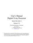
The DXP can accommodate most common x-ray detector preamplifiers, and is especially well suited for
single or multi-element Si(Li) and germanium detectors with pulsed optical reset (POR) preamplifiers. A typical
multi-element detector array system equipped with DXP readout is shown in Figure 1.1.
X-ray Detector
(19 element)
CAMAC
Mini-Crate
Host Computer
(Mac,PC,...)
CRATE
CONTROLLER
PREAMP
POWER
TIMING CONTROL
DXP
DXP
DXP
DXP
DXP
SCSI
Figure 1.1: Schematic of a 19 element x-ray detector read out using 5 DXP modules. Each preamplifier has one
input signal into a DXP channel. The preamplifiers can all be powered from the same CAMAC
crate. A timing control module is shown to synchronize the data taking. The host processor can
control the CAMAC system via numerous methods.
The DXP will accommodate either positive or negative polarity input signals, as selected by an internal
jumper, which only needs to be set initially or when switching between different polarity preamplifiers. With
POR preamplifiers, the standard DXP channel accepts signals with a peak to peak reset range of up to 6 volts
and a mean value between +2 V and - 2 V. This range can be extended by modifying the input buffer amplifiers’
gain: please contact XIA if needed. To maximize dynamic range, an offset reference voltage from a DAC is used
to center the reset ramp signal at 0 volts following the input buffer amplifier stage. Touch points allow this
signal to be measured at the front panel for each channel.
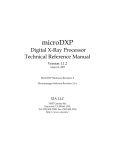
Each DXP board can have 1 to 4 channels and so accommodate up to four preamplifier channels per
module. Each channel consists of four basic sections, shown below in Figure 1.2: a front-end Analog Signal
Conditioner (ASC); an ADC digitizing at 20 MHz; a digital Filter, Peak detector, Pileup Inspector (FiPPI) to filter
the digitized signal stream and capture x-ray events; and a Digital Signal Processor (DSP) for pulse height
analysis, data corrections, control of the other system sections (ASC & FiPPI), and communication with a host
processor.
Analog Signal
Digital Filter &
Conditioner
Pile-up Rejector
(ASC)
IN
+
-
+
Subtractor
Function
Generator
Processor
(FiPPI)
Variable
Gain
Buffer
Digital Signal
(DSP)
Data
Low
Pass
Filter
ADC
Data
Fast
Slow
Good
Peak Measure,
MCA Binning &
ASC Control
Quad DAC
Interface to
Control Computer
Figure 1.2: Block diagram of the DXP channel architecture, showing the major functional sections.
July 27, 2000
Page 3
Manual: DXP 4C/4T
mdo-DXP-MAN-001.3
The preamplifier output signal feeds in to the ASC via a front panel LEMO connector with 1000
impedance. The role of the ASC is to match the signals from a wide variety of commonly used preamplifiers to
the range and sampling rate of the ADC. It does this by subtracting an offset signal, which in the case of reset
preamplifiers is an internally generated ramp signal, and scaling the difference by a programmable gain. The
DSP monitors the ASC’s behavior, periodically adjusts the control DACs, and detects preamplifier resets to reset
the internal ramp generator. Before being digitized the signal bandwidth is limited with a Butterworth low-pass
filter to meet the Nyquist criterion.
The FiPPI utilizes a pair of trapezoidal filters: the "fast" filter, with a short peaking time for event
selection and pile-up rejection; and the "slow" filter, with a longer peaking time for better energy resolution.
[Note that a triangularly shaped pulse of peaking time t has approximately the same duration as a semiGaussian shaped pulse of shaping time t/2.] Both trapezoidal filters have programmable peaking times and
gaps, where the gap (or "flat top") can be adjusted to compensate for preamp rise times (to avoid problems
caused by "ballistic deficit"). The use of the fast filter and digital pile-up inspection decreases the dead-time per
event to be just the pulse base-width (i.e. twice the peaking time + gap), which is less than the dead time for
comparable analog systems. For the shortest peaking time (0.5 µsec) an output count rate of more than 300 kHz
can be achieved. Fast filter parameters such as the discriminator threshold and pile-up rejection criteria are
completely programmable. The FiPPI has been implemented in a Xilinx field programmable gate array (FPGA),
and thus may be reprogrammed for special purposes.
The DSP, optimized for fixed point arithmetic and high I/O rate, applies data corrections to achieve
optimal resolution with either pulsed optical reset or resistor feedback preamplifiers. While collecting data, the
DSP continually monitors and controls the ASC output to match the ADC input range. The DSP operates at up
to the highest event rates with very low dead-time from processor overhead. Other sources of dead-time (such as
preamplifier resets) tend to be larger. In any case, the total live-time during data taking is accurately recorded.
The total number of fast-peak triggers (i.e. the measured ICR) is also recorded to allow precise correction for
dead-time due to pulse pile-up.
The standard software for the DSP processors includes a program for internal calibration and
spectroscopy measurements, which collects spectra in a separate 1024 bin MCA for each detector channel. This
software can be customized for special purposes; interested persons should contact XIA for further information.
The DSP software is described in the DSP Software Manual [Ref. 1]. In addition, the control software running
on the host computer is an important part of the system. Several options exist for implementations on different
platforms. XIA has developed a suite of driver routines using LabVIEW for the Macintosh, as described in the
LabView Software Description Manual [Ref. 2]. These can be used for standalone data acquisition or as a
networked data server via TCP/IP. They can relatively easily be ported to Windows PC's or other platforms for
which LabVIEW has been implemented. Alternatively, a set of C and FORTRAN callable driver routines been
developed to assist those who wish to integrate DXP control into their existing data collection programs. These
are described in the Host Software Description Manual [Ref. 3]. Work is currently underway to integrate the
host software with other available XAS control software packages including EPICS and SPEC. Please contact
XIA or XIA’s web site (www.xia.com) for further details on these and other options.
The DXP Model 4C module has an external TTL gate signal (Ext_Gate) to provide the option of
controlling data acquisition from an external timing source, such as a CAMAC real time clock. Model 4T has a
second TTL input (Ext_Sync) which may be used for various special purposes, as described in Appendix E.
These include switching data collection between multiple spectra in the DSP synchronously with some external
experimental parameter (e.g. phase locked EXAFS), and time resolved multichannel scaling, including “quickEXAFS”. Either model can be equipped with up to 32 KBytes of additional memory per channel, for larger
spectra or other special applications.
July 27, 2000
Page 4
Manual: DXP 4C/4T
mdo-DXP-MAN-001.4
2. Digital Filtering Theory, DXP Structure and Theory of Operation:
The purpose of this section is to provide the general DXP user with an explanation of its operation
which is deep and complete enough to allow the module to be used effectively yet not so filled with detail as to
become cumbersome. A further level of detail is required for those who wish to engage in developing control
programs for the DXP and this is provided in the companion volumes DSP Software Manual for the DXP 4C/4T
Digital X-ray Processor [Ref. 1] and Host Software Description Manual for the DXP 4C/4T Digital X-ray Processor
[Ref. 3].
This introduction is divided into three sections. In the first, we examine the general issues associated
with using a digital processor to extract accurate x-ray energies from a preamplifier signal and detect and
eliminate pile-ups. In the second section we then describe how these general functions are specifically
implemented in the DXP. This leads rather naturally to a discussion of the parameters used to control the
DXP’s functions: that is, those digital values which replace knob positions in analog systems. In the third
section we the proceed to describe strategies both for selecting reasonable starting parameter values and for
adjusting their values to optimize performance in particular situations.
2.1. X-ray Detection and Preamplifier Operation:
Energy dispersive detectors, which include such solid state detectors as Si(Li), HPGe, HgI2, CdTe and
CZT detectors, are generally operated with charge sensitive preamplifiers as shown in Figure 2.1a. Here the
detector D is biased by voltage source V and connected to the input of amplifier A which has feedback capacitor
Cf. In resetting preamplifiers a switch S is provided to short circuit Cf from time to time when the amplifier’s
output voltage gets so large that it behaves nonlinearly. Switch S may be an actual transistor switch, or may
operate equivalently by another mechanism. In pulsed optical reset preamps light is shined on the amplifier A’s
input FET to cause it to discharge Cf. In PentaFET circuits, the input FET has an additional electrode which can
be pulsed to discharge Cf.
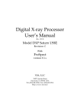
The output of the preamplifier following the absorption of an x-ray of energy Ex in detector D is shown
in Figure 2.1b as a step of amplitude Vx. When the x-ray is absorbed in the detector material it releases an
electric charge Qx = Ex/ε, where ε is a material constant. Qx is integrated onto Cf, to produce the voltage Vx =
Qx/Cf = Ex/(εCf). Measuring the energy Ex of the x-ray therefore requires a measurement of the voltage step Vx
in the presence of the amplifier noise σ, as indicated in Fig. 2.1b.
V
S
C
D
A
f
Preamp Output (mV)
4
2
Vx
0
σ
-2
-4
0.00
a)
b)
0.02
0.04
0.06
Time (ms)
Figure 2.1: a) Charge sensitive preamplifier with reset; b) Output on absorption of an x-ray.
July 27, 2000
Page 5
Manual: DXP 4C/4T
mdo-DXP-MAN-001.4
2.2. X-ray Energy Measurement & Noise Filtering:
Reducing noise in an electrical measurement is accomplished by filtering. Traditional analog filters use
combinations of a differentiation stage and multiple integration stages to convert the preamp output steps, such
as shown in Fig. 2.1b, into either triangular or semi-Gaussian pulses whose amplitudes (with respect to their
baselines) are then proportional to Vx and thus to the x-ray’s energy.
Digital filtering proceeds from a slightly different perspective. Here the signal has been digitized and is
no longer continuous, but is instead a string of discrete values, such as shown in Figure 2.2. Fig. 2.2 is actually
just a subset of Fig. 2.1b, which was dititized by a Tektronix 544 TDS digital oscilloscope at 10 MSA
(megasamples/sec). Given this data set, and some kind of arithmetic processor, the obvious approach to
determining Vx is to take some sort of average over the points before the step and subtract it from the value of the
average over the points after the step. That is, as shown in Fig. 2.2, averages are computed over the two regions
marked “Length” (the “Gap” region is omitted because the signal is changing rapidly here), and their difference
taken as a measure of Vx. Thus the value Vx may be found from the equation:
Vx ,k =
–
Σ
i (before
w i vi +
)
Σ
wi vi
(2.1)
i ( after )
where the values of the weighting constants wi determine the type of average being computed. The sums of the
values of the two sets of weights must be individually normalized.
Preamp Output (mV)
4
2
Length
Gap
0
Length
-2
Digitized Step 960919
-4
20
22
24
26
28
30
Time ( µs)
Figure 2.2: Digitized version of the data of Fig. 3B in the step region.
The primary differences between different digital signal processors lie in two areas: what set of weights
{wi} is used and how the regions are selected for the computation of Eqn. 2.1. Thus, for example, when the
weighting values decrease with separation from the step, then Eqn. 2.1 produces “cusp-like” filters. When the
weighting values are constant, one obtains triangular (if the gap is zero) or trapezoidal filters. The concept
behind cusp-like filters is that, since the points nearest the step carry the most information about its height, they
should be most strongly weighted in the averaging process. How one chooses the filter lengths results in time
variant (the lengths vary from pulse to pulse) or time invariant (the lengths are the same for all pulses) filters.
Traditional analog filters are time invariant. The concept behind time variant filters is that, since the x-rays
arrive randomly and the lengths between them vary accordingly, one can make maximum use of the available
information by setting Length to the interpulse spacing.
July 27, 2000
Page 6
Manual: DXP 4C/4T
mdo-DXP-MAN-001.4
In principal, the very best filtering is accomplished by using cusp-like weights and time variant filter
length selection. There are serious costs associated with this approach however, both in terms of computational
power required to evaluate the sums in real time and in the complexity of the electronics required to generate
(usually from stored coefficients) normalized {wi} sets on a pulse by pulse basis. A few such systems have been
produced but typically cost about $13K per channel and are count rate limited to about 30 Kcps. Even time
invariant systems with cusp-like filters are still expensive due to the computational power required to rapidly
execute strings of multiply and adds. One commercial system exists which can process over 100 Kcps, but it too
costs over $12K per channel.
The DXP processing system developed by XIA takes a different approach because it was optimized for
very high speed operation and low cost per channel. It implements a fixed length filter with all wi values equal
to unity and in fact computes this sum afresh for each new signal value k. Thus the equation implemented is:
Σ
k – L – G
L V x ,k =
–
i = k – 2L – G + 1
Σ
k
vi +
i = k – L + 1
vi
,
(2.2)
where the filter length is L and the gap is G. The factor L multiplying Vx,k arises because the sum of the weights
here is not normalized. Accommodating this factor is trivial for the DXP’s host software. In the DXP, Eqn. 2.2 is
actually implemented in hardwired logic by noting the recursion relationship between Vx,k and Vx,k-1, which
is:
L Vx,k = L Vx,k-1 + vk - vk-L - vk-L-G + vk-2L-G
(2.3)
While this relationship is very simple, it is still very effective. In the first place, this is the digital equivalent of
triangular (or trapezoidal if G 0) filtering which is the analog industry’s standard for high rate processing. In
the second place, one can show theoretically that if the noise in the signal is white (i.e. Gaussian distributed)
above and below the step, which is typically the case for the short shaping times used for high signal rate
processing, then the average in Eqn. 2.2 actually gives the best estimate of Vx in the least squares sense. This, of
course, is why triangular filtering has been preferred at high rates. Triangular filtering with time variant filter
lengths can, in principle, achieve both somewhat superior resolution and higher throughputs but comes at the
cost of a significantly more complex circuit and a rate dependent resolution, which is unacceptable for many
types of precise analysis. In practice, XIA’s design has been found to duplicate the energy resolution of the best
analog shapers while approximately doubling their throughput, providing experimental confirmation of the
validity of the approach.
2.3. Trapezoidal Filtering in the DXP:
From this point onward, we will only consider trapezoidal filtering as it is implemented in the DXP
according to Eqns. 2.2 and 2.3. The result of applying such a filter with Length L = 20 and Gap G = 4 to the
same data set of Fig. 2.2 is shown in Figure 2.3. The filter output Vx is clearly trapezoidal in shape and has a
risetime equal to L, a flattop equal to G, and a symmetrical falltime equal to L. The basewidth, which is a firstorder measure of the filter’s noise reduction properties, is thus 2L+G. This raises several important points in
comparing the noise performance of the DXP to analog filtering amplifiers. First, semi-Gaussian filters are
usually specified by a shaping time . Their peaking time is typically twice this and their pulses are not symmetric
so that the basewidth is about 5.6 times the shaping time or 2.8 times their peaking time. Thus a semi-Gaussian
filter typically has a slightly better energy resolution than a triangular filter of the same peaking time because it
has a longer filtering time. This is typically accommodated in amplifiers offering both triangular and semiGaussian filtering by stretching the triangular peaking time a bit, so that the true triangular peaking time is
typically 1.2 times the selected semi-Gaussian peaking time. This also leads to an apparent advantage for the
analog system when its energy resolution is compared to a digital system with the same nominal peaking time.
One extremely important characteristic of a digitally shaped trapezoidal pulse is its extremely sharp
termination on completion of the basewidth 2L+G. This may be compared to analog filtered pulses which have
tails which may persist up to 40% of the peaking time, a phenomenon due to the finite bandwidth of the analog
filter. As we shall see below, this sharp termination gives the digital filter a definite rate advantage in pileup
free throughput.
July 27, 2000
Page 7
Manual: DXP 4C/4T
mdo-DXP-MAN-001.4
6
Filtered Step S.kfig 960920
Output (mV)
4
2
0
L
L+G/2
2L+G
-2
Preamp Output (mV)
Filter Output (mV)
-4
24
26
28
Time (
30
32
µs)
Figure 2.3: Trapezoidal filtering the Preamp Output data of Fig. 2.2 with L = 20 and G = 4.
2.4. Baseline Issues:
Figure 2.4 shows the same event as is Fig. 2.3 but over a longer time interval to show how the filter treats
the preamplifier noise in regions when no x-ray pulses are present. As may be seen the effect of the filter is both
to reduce the amplitude of the fluctuations and reduce their high frequency content. This signal is termed the
baseline because it establishes the reference level from which the x-ray peak amplitude Vx is to be measured.
The fluctuations in the baseline have a standard deviation σe which is referred to as the electronic noise of the
system, a number which depends on the peaking time of the filter used. Riding on top of this noise, the x-ray
peaks contribute an additional noise term, the Fano noise , which arises from statistical fluctuations in the
amount of charge Qx produced when the x-ray is absorbed in the detector. This Fano noise σf adds in
quadrature with the electronic noise, so that the total noise σt in measuring Vx is found from
σt = sqrt( σf2 + σe2 ).
(2.4)
The Fano noise is only a property of the detector material. The electronic noise, on the other hand, may have
contributions from both the preamplifier and the amplifier. When the preamplifier and amplifier are both well
designed and well matched, however, the amplifier’s noise contribution should be essentially negligible.
Achieving this in the mixed analog-digital environment of a digital pulse processor is a non-trivial task,
however.
In the general case, however, the mean baseline value in not zero. This situation arises whenever the
slope of the preamplifier signal it not zero between x-ray pulses. This can be seen from Eqn. 2.2. When the slope
is not zero, the mean values of the two sums will differ because they are taken over regions separated in time by
L+G, on average. Such non-zero slopes can arise from various causes, of which the most common is detector
leakage current.
July 27, 2000
Page 8
Manual: DXP 4C/4T
mdo-DXP-MAN-001.4
When the mean baseline value is not zero, it must be determined and subtracted from measured peak
values in order to determine Vx values accurately. If the error introduced by this subtraction is not to
significantly increase σt, then the error in the baseline estimate σb must be small compared to σe. Because the
error in a single baseline measurement will be σe, this means that multiple baseline measurements will have to
be averaged. In the standard DXP operating code this number is 64, which leads to the total noise shown in
Eqn. 2.5.
σt = sqrt( σf2 + (1+1/64)σe2 ).
(2.5)
This results in less than 0.5 eV degradation in resolution even for very long peaking times when resolutions of
order 140 eV are obtained.
In practice, the DXP initially makes a series of 64 baseline measurements to compute a starting baseline
mean. It then makes additional baseline measurements at quasi-periodic intervals to keep the estimate up to
date. These values are stored internally and can be read out to construct a spectrum of baseline noise. This is
recommended because of its excellent diagnostic properties. When all components in the spectrometer system
are working properly, the baseline spectrum should be Gaussian in shape with a standard deviation reflecting
σn . Deviations from this shape indicate various pathological conditions which also cause the x-ray spectrum to
be distorted and which should be fixed.
6
Filtered Step L.kfig 960920
σt
4
Output (mV)
V
2
x
σe
0
-2
Preamp Output (mV)
Filter Output (mV)
-4
5
10
15
20
25
Time (
30
35
40
45
µs)
Figure 2.4: The event of Fig. 2.3 displayed over a longer time period to show baseline noise.
2.5. X-ray Detection & Threshold Setting:
As noted above, we wish to capture a value of Vx for each x-ray detected and use these values to
construct a spectrum. This process is also significantly different between digital and analog systems. In the
analog system the peak value must be “captured” into an analog storage device, usually a capacitor, and “held”
until it is digitized. Then the digital value is used to update a memory location to build the desired spectrum.
July 27, 2000
Page 9
Manual: DXP 4C/4T
mdo-DXP-MAN-001.4
During this analog to digital conversion process the system is dead to other events, which can severely reduce
system throughput. Even single channel analyzer systems introduce significant deadtime at this stage since
they must wait some period (typically a few microseconds) to determine whether or not the window condition is
satisfied.
Digital systems are much more efficient in this regard, since the values output by the filter are already
digital values. All that is required is to capture the peak value – it is immediately ready to be added to the
spectrum. If the addition process can be done in less than one peaking time, which is usually trivial digitally,
then no system deadtime is produced by the capture and store operation. This is a significant source of the
enhanced throughput found in digital systems.
In the DXP the peak detection and sampling is handled as indicated in Figure 2.5. In the DXP two
trapezoidal filters are implemented, a fast filter and a slow filter. The fast filter is used to detect the arrival of xrays, the slow filter is used to reduce the noise in the measurement of Vx, as described in the sections above. Fig.
2.5 shows the same data as in Figs. 2.1 - 2.4, together with the normalized fast and slow filter outputs. The fast
filter has a filter length Lf = 4 and a gap Gf = 0. The slow filter has Ls = 20 and Gs = 4. Because the samples
were taken at 10 MSA, these correspond to peaking times of 400 ns and 2 µs, respectively.
F/S Filtered Data kfig 960920
20
Preamp
16
Offset Outputs (mV)
"Arrival Time"
12
MINWIDTH = 3
THRESHOLD
Fast Filter
8
PEAKSAMP
"Sampling Time"
4
Slow Filter
0
20
22
24
26
Time (
28
30
32
µs )
Figure 2.5: Peak detection and sampling methods in the DXP digital processor.
The arrival of the x-ray step (in the preamp output) is detected by digitally comparing the fast filter
output to the digital constant THRESHOLD, which represent a threshold value. Once the threshold is exceeded,
the number of values above threshold are counted. If they exceed a minimum number MINWIDTH, then the
excursion is classified as a true peak and not a noise fluctuation. This scheme is much more noise resistant
than a simple discriminator circuit, which triggers anytime the threshold is crossed. Thus THRESHOLD can be
set much closer to the noise floor, which can be particularly advantageous when working with low energy xrays. Once the MINWIDTH criterion has been satisfied, the DXP finds the arrival of the largest value (which
July 27, 2000
Page 10
Manual: DXP 4C/4T
mdo-DXP-MAN-001.4
becomes the pulse’s official “arrival time”) and starts a counter to count PEAKSAMP clock cycles to arrive at the
appropriate time to sample the value of the slow filter. Because the digital filtering processes are deterministic,
PEAKSAMP depends only on the values of the fast and slow filter constants and the risetime of the preamplifier
pulses. The slow filter value captured following PEAKSAMP is then the slow digital filter’s estimate of Vx.
2.6. Pile-up Inspection:
The value Vx captured at time PEAKSAMP after the x-ray pulse’s arrival time will only be a valid
measure of the associated x-ray’s energy provided that the filtered pulse is sufficiently well separated in time
from its preceding and succeeding neighbor pulses so that their peak amplitudes are not distorted by the action
of the trapezoidal filter. That is, if the pulse is not piled up. The relevant issues may be understood by reference
to Figure 2.6, which shows 5 x-rays arriving separated by various intervals.
Because the triangular filter is a linear filter, its output for a series of pulses is the linear sum of its
outputs for the individual members in the series. In Fig. 2.6 the pulses are separated by intervals of 3.2, 1.8, 5.7,
and 0.7 µs, respectively. The fast filter has a peaking time of 0.4 µs with no gap. The slow filter has a peaking
time of 2.0 µs with a gap of 0.4 µs.
The first kind of pileup is slow pileup, which refers to pileup in the slow channel. This occurs when the
rising (or falling) edge of one pulse lies under the peak (specifically the sampling point) of its neighbor. Thus, in
Fig. 2.6, peaks 1 and 2 are sufficiently well separated so that the leading edge (point 2a) of peak 2 falls after the
peak of pulse 1. Because the trapezoidal filter function is symmetrical, this also means that pulse 1’s trailing
edge (point 1c) also does not fall under the peak of pulse 2. For this to be true, the two pulses must be separated
by at least an interval of L + G/2. Peaks 2 and 3, which are separated by only 1.8 µs, are thus seen to pileup in
the present example with a 2.0 µs peaking time.
This leads to an important first point: whether pulses suffer slow pileup depends critically on the
peaking time of the filter being used. The amount of pileup which occurs at a given average signal rate will
increase with longer peaking times. We will quantify this in §2.6.
Because the fast filter peaking time is only 0.4 µs, these x-ray pulses do not pileup in the fast filter
channel. The DXP can therefore test for slow channel pileup by measuring for the interval PEAKINT after a
pulse arrival time. If no second pulse occurs in this interval, then there is no trailing edge pileup. PEAKINT is
usually set to a value close to L + G/2 + 1. Pulse 1 passes this test, as shown in Fig. 2.6. Pulse 2, however, fails
the PEAKINT test because pulse 3 follows in 1.8 µs, which is less than PEAKINT = 2.3 µs. Notice, by the
symmetry of the trapezoidal filter, if pulse 2 is rejected because of pulse 3, then pulse 3 is similarly rejected
because of pulse 2.
Pulses 4 and 5 are so close together that the output of the fast filter does not fall below the threshold
between them and so they are detected by the pulse detector as only being a single x-ray pulse. Indeed, only a
single (though somewhat distorted) pulse emerges from the slow filter, but its peak amplitude corresponds to
the energy of neither x-ray 4 nor x-ray 5. In order to reject as many of these fast channel pileup cases as possible,
the DXP implements a fast channel pileup inspection test as well.
The fast channel pileup test is based on the observation that, to the extent that the risetime of the
preamplifier pulses is independent of the x-rays’ energies (which is generally the case in x-ray work except for
some room temperature, compound semiconductor detectors) the basewidth of the fast digital filter (i.e. 2Lf + Gf)
will also be energy independent and will never exceed some maximum width MAXWIDTH. Thus, if the width
of the fast filter output pulses is measured at threshold and found to exceed MAXWIDTH, then fast channel
pileup must have occurred. This is shown graphically in Fig. 2.6, where pulse 3 passes the MAXWIDTH test,
while the piled up pair of pulses 4 and 5 fail the MAXWIDTH test.
Thus, in Fig. 2.6, only pulse 1 passes both pileup inspection tests and, indeed, it is the only pulse to
have a well defined flattop region at time PEAKSAMP in the slow filter output.
July 27, 2000
Page 11
Manual: DXP 4C/4T
25
mdo-DXP-MAN-001.4
Digitized MultiPile kfig 960921
4
20
2
1
Preamp
5
3
Passes
PEAKINT
Test
Fails
PEAKINT
Test
Passes
MAXWIDTH
Test
15
Fails
MAXWIDTH
Test
Fast Filter
10
4
2
1
5
3
PEAKSAMP
5
1b
1a
2a
1c
Slow Filter
0
5
10
15
20
Time (
25
30
µ s)
Figure 2.6: A sequence of 5 x-ray pulses separated by various intervals to show the origin of both slow channel
and fast channel pileup and demonstrate how the two cases are detected by the DXP.
2.7. Input Count Rate (ICR) and Output Count Rate (OCR):
During data acquisition, x-rays will be absorbed in the detector at some rate. This is the true input count
rate , which we will refer to as ICR t. Because of fast channel pileup, not all of these will be detected by the DXP’s
x-ray pulse detection circuitry, which will thus report a measured input count rate ICR m which will be less than
ICR t. This phenomenon, it should be noted, is a characteristic of all x-ray detection circuits, whether analog or
digital, and is not specific to the DXP.
Of the detected x-rays, some fraction will also satisfy both fast and slow channel pileup tests and have
their values of Vx captured and placed into the spectrum. This number is the output count rate , which we refer to
as the OCR. The DXP normally returns, in addition to the collected spectrum, the actual time LIVETIME for
which data was collected, together with the number FASTPEAKS of fast peaks detected and the number of Vx
captured events EVTSINRUN. From these values, both the OCR and ICR m can be computed according to
Equation 6. These values can then be used to make deadtime corrections as discussed in the next section.
ICR m = FASTPEAKS/LIVETIME; OCR = EVTSINRUN/LIVETIME.
July 27, 2000
(2.6)
Page 12
Manual: DXP 4C/4T
mdo-DXP-MAN-001.4
2.8. Throughput:
Figure 2.7 shows how the values of ICR m and OCR vary with true input count rate for the DXP and
compare these results to those from a common analog shaping amplifier plus SCA system. The data were taken
at a synchrotron source using a detector looking at a CuO target illuminated by x-rays slightly above the Cu K
edge. Intensity was varied by scanning a pair of slits across the input x-ray beam so that its harmonic content
remained constant with varying intensity.
200
DXP OCR
DXP ICR
m
Analog OCR
Analog ICR
Output Count Rate (kcps)
150
True ICR
m
t
100
50
ICR/OCR Plot kfig 960922
0
0
50
100
150
200
Input Count Rate (kcps)
System
OCR Deadtime (µ
µ s)
ICR Deadtime (µ
µ s)
DXP (2 µ s τp, 0.6 µs τg)
4.73
0.83
Analog Triangular Filter Amp (τp = 1 µ s)
4.47
0.40
Figure 2.7: Curves of ICR m and OCR for the DXP using 2 µs peaking time, compared to a common analog SCA
system using 1 µs peaking time.
Functionally, the OCR in both cases is seen to initially rise with increasing ICR and then saturate at
higher ICR levels. The theoretical form, from Poisson statistics, for a channel which suffers from paralyzable
(extending) dead time [Ref. 4], is given by:
OCR = ICR t * exp( - ICR t τd ),
(2.7)
where τd is the dead time. Both the DXP and analog systems’ OCRs are so describable, with the slow channel dead
times τds shown in the Table below Fig. 2.7. The measured ICR m values for both the DXP and analog systems
are similarly describable, with the fast channel dead times τdf as shown. The maximum value of OCR can be
found by differentiating Eqn. 2.7 and setting the result to zero. This occurs when the value of the exponent is -1,
i.e. when ICR t equals 1/τd. At this point, the maximum OCR max is 1/e the ICR, or
July 27, 2000
Page 13
Manual: DXP 4C/4T
mdo-DXP-MAN-001.4
OCR max = 1/(e τd) = 0.37/τd.
(2.8)
These are general results and are very useful for estimating experimental data rates.
The Table illustrates a very important result for using the DXP: the slow channel deadtime is nearly the
minimum theoretically possible, namely the pulse basewidth. For the shown example, the basewidth is 4.6 µs
(2Ls + Gs ) while the deadtime is 4.73 µs. The slight increase is because, as noted above, PEAKINT is always set
slightly longer than Ls - Gs /2 to assure that pileup does not distort collected values of Vx.
The deadtime for the analog system, on the other hand is much larger. In fact, as shown, the
throughput for the digital system is almost twice as high, since it attains the same throughput for a 2 µs peaking
time as the analog system achieves for a 1 µs peaking time. The slower analog rate arises, as noted earlier both
from the longer tails on the pulses from the analog triangular filter and on additional deadtime introduced by
the operation of the SCA. In spectroscopy applications where the system can be profitably run at close to
maximum throughput, then, a single DXP channel will then effectively count as rapidly as two analog
channels.
2.9. Dead Time Corrections:
The fact that both OCR and ICR m are describable by Eqn. 2.7 makes it possible to correct DXP spectra
quite accurately for deadtime effects. Because deadtime losses are energy independent, the measured counts
Nmi in any spectral channel i are related to the true number Nti which would have been collected in the same
channel i in the absence of deadtime effects by:
Nti = Nmi ICR t/OCR.
(2.9)
Looking at Fig. 2.7, it is clear that a first order correction can be made by using ICR m in Eqn. 2.9 instead of ICR t,
particularly for OCR values less than about 50% of the maximum OCR value. For a more accurate correction,
the fast channel deadtime τdf should be measured from a fit to the equation
ICR m = ICTt * exp( - ICR t τdf ).
(2.10)
Then, for each recorded spectrum, the associated value of ICR m is noted and Eqn. 2.10 inverted (there are simple
numerical routines to do this for transcendental equations) to obtain ICR t. Then the spectrum can be corrected
on a channel by channel basis using Eqn. 2.9. In experiments with a DXP prototype, we found that, for a 4 µs
peaking time (for which the maximum ICR is 125 kcps), we could correct the area of a reference peak to better
than 0.5% between 1 and 120 kcps. The fact that the DXP provides highly accurate measurements of both
LIVETIME and ICR m therefore allows it to produce accurate spectral measurements over extremely wide ranges
of input counting rates.
July 27, 2000
Page 14
Manual: DXP 4C/4T
mdo-DXP-MAN-001.4
This page intentionally blank.
July 27, 2000
Page 15
Manual: DXP 4C/4T
mdo-DXP-MAN-001.4
3. DXP Structure and Description of Operation:
3.1. Organizational Overview:
For convenience, Fig. 1.2 is repeated here as Figure 3.1, showing the three major operating blocks in the
DXP: the Analog Signal Conditioner (ASC), Digital Filter, Peak Detector, and Pileup Inspector (FiPPI), and
Digital Signal Processor (DSP). Signal digitization occurs in the Analog-to-Digital converter (ADC), which lies
between the ASC and the FiPPI. In the DXP, the ADC is a 10 bit, 20 MSA device. The functions of the major
blocks are summarized below.
Analog Signal
Conditioner
(ASC)
IN
Digital Signal
Processor
(DSP)
Variable
Buffer
+
-
Digital Filter, Pulse
Detector, & Pile-up Inspector
(FiPPI)
Gain
Data
+
Data
Low
Subtractor
Pass
-
ADC
Filter
Sawtooth
Slow
Peak Measure,
MCA Binning &
Function
Generator
Fast
Reset
Good
ASC Control
Gain DAC
Slope DAC
Tracking DAC
Interface to
Control Computer
Offset DAC
System Dwg 960924
Figure 3.1: Block diagram of the DXP channel architecture, showing the major functional sections.
3.2. The Analog Signal Conditioner (ASC):
The ASC has two major functions: to reduce the dynamic range of the input signal so that it can be
adequately digitized by a 10 bit converter and to reduce the bandwidth of the resultant signal to meet the
Nyquist criterion for the following ADC. This criterion is that there should be no frequency component in the
signal which exceeds half of the sampling frequency. Frequencies above this value are aliased into the digitized
signal at lower frequencies where they are indistinguishable from original components at those frequencies. In
particular, high frequency noise would appear as excess low frequency noise, spoiling the spectrometer’s
energy resolution. The DXP therefore has a 4 pole Butterworth filter with a cutoff frequency of about 8 MHz.
The dynamic range of the preamplifier output signal is reduced to allow the use of a 10 bit ADC, which
greatly lowers the cost of the DXP. This need arises from two competing ADC requirements: speed and
resolution. Speed is required to allow good pulse pileup detection, as described in §2.5. For high count rates,
pulse pair resolution less than 200 ns is desirable, which implies a sampling rate of 10 MSA or more. The DXP
uses a 20 MSA ADC. On the other hand, in order to reduce the noise σ in measuring Vx (see Fig. 2.1), experience
shows that σ must be at least 4 times the ADC’s single bit resolution ∆V1 . This effectively sets the gain of the
amplifier stages preceding the ADC. Then, if the preamplifier’s full scale voltage range is Vmax, it must digitize
to N bits, where N is given by:
N = log 10 (Vmax/∆V1 )/log 10 (2).
July 27, 2000
(11)
Page 16
Manual: DXP 4C/4T
mdo-DXP-MAN-001.4
For a typical high resolution spectrometer, N must be 14 to 15. However, 14 bit ADCs operating in excess of 10
MSA are very expensive, particularly if their integral and differential non-linearities are less than 1 least
significant bit (LSB). At the time of this writing a 10 bit 20 MSA ADC costs less than $10, while a 14 bit 5 MSA
ADC costs nearly $500, which would more than triple the parts cost per channel.
The ASC circumvents this problem using a novel dynamic range technology, for which XIA has applied
for a patent, which is indicated in Figure 3.2. Here a resetting preamplifier output is shown which cycles
between about -3.0 and -0.5 volts. We observe that it is not the overall function which is of interest, but rather
the individual steps, such as shown in Fig. 2.1b, which carry the x-ray amplitude information. Thus, if we
know the average slope of the preamp output, we can generate a sawtooth function which has this average
slope and restarts each time the preamplifier is reset, as shown in Fig. 3.2. If we then subtract this sawtooth
from the preamplifier signal, we can amplify the difference signal to match the ADC’s input range, also as
indicated in the Figure. Gains of 8 to 16 are possible, thus reducing the required number of bits
ADC Max Input
3.0
2.0
Amplified Sawtooth Subtracted Data
Preamp Output (V)
1.0
ADC Min Input
Preamp
Output
0.0
-1.0
-2.0
Sawtooth
Function
Reset
Level
-3.0
0
Preamp-Sawtooth kfig 960923
1
2
3
4
5
Time (ms)
Figure 3.2: A sawtooth function having the same average slope as the preamp output is subtracted from it and
the difference amplified and offset to match the input range of the ADC.
from 14 to 10. The generator required to produce this sawtooth function is quite simple, comprising a current
integrator with an adjustable offset. The current, which sets the slope, is controlled by a DAC (SLOPEDAC),
July 27, 2000
Page 17
Manual: DXP 4C/4T
mdo-DXP-MAN-001.4
while the offset is controlled by a second DAC (TRACKDAC). The DAC input values are set by the DSP, which
thereby gains the power to adjust the sawtooth generator in order to maintain the ASC output (i.e. the
“Amplified Sawtooth Subtracted Data” of Fig. 3.2) within the ASC input range.
Occasionally, as also shown in Fig. 3.2, fluctuations in data arrival rate will cause the conditioned
signal to pass outside the ADC input range. This condition is detected by the FiPPI, which has digital
discrimination levels set to ADC zero and full scale, which then interrupts the DSP, demanding ASC attention.
The DSP remedies the situation by adjusting TRACKDAC until the conditioned signal returns into the ADC’s
input range. During this time, data passed to the FiPPI are invalid. Preamplifier resets are detected similarly.
When detected the DSP responded by setting TRACKDAC to a standard value corresponding the reset level
(TRACKRST) and resetting the current integrator.
3.3. The Filter, Pulse Detector, & Pile-up Inspector (FiPPI):
The FiPPI is implemented in a field programmable gate array (FPGA) to accomplish the various
filtering, pulse detection and pileup inspection tasks discussed in §2. As described there, it has a fast channel
for pulse detection and pileup inspection and a slow channel for filtering, both with fully adjustable peaking
times and gaps. The "fast" filter’s τp (τpf) can be adjusted from 100 ns to 1.25 µs, while the "slow" filter’s τp (τps)
can be adjusted from 0.5 µs to 20 µs. Adjusting τpf allows tradeoffs to be made between pulse pair resolution
and the minimum x-ray energy that can be reliably detected. When τpf is 200 ns, for example, the pulse pair
resolution is typically less than 200 ns. When τpf is 1 µs, x-rays with energies below 200 eV can be detected and
inspected for pileup. To maximize throughput, τps should be chosen to be as short as possible to meet energy
resolution requirements, since the maximum throughput scales as 1/τps, as per Eqn. 2.8. If the input signal
displays a range of risetimes (as in the “ballistic deficit” phenomenon) the slow filter gap time can be extended
to accommodate that range. The shortest value of τps 0.5 µs, is set by the response time of the DSP to the FiPPI
when a value of Vx is captured. At this setting, however, with a gap time of 100 ns, the dead time would be
about 1.2 µs and the maximum throughput according to Eqn. 2.8 would be 310 kcps.
The FiPPI also includes a livetime counter which counts the 20 MHz system clock, divided by 16, so
that one “tick” is 800 ns. This counter is activated any time the DSP is enabled to collect x-ray pulse values from
the FiPPI and therefore provides an extremely accurate measure of the system livetime. In particular, as
described in §3.2, the DSP is not live either during preamplifier resets or during ASC out-of-ranges, both because
it is adjusting the ASC and because the ADC inputs to the FiPPI are invalid. Thus the DXP measures livetime
more accurately than an external clock, which is insensitive to resets and includes them as part of the total
livetime. While the average number of resets/sec scales linearly with the countrate, in any given measurement
period there will be fluctuations in the number of resets which may affect counting statistics in the most precise
measurements.
All FiPPI parameters, including the filter peaking and gap times, threshold, and pileup inspection
parameters are all externally supplied and may be adjusted by the user to optimize performance. Because the
FiPPI is implemented in a Xilinx field programmable gate array (FPGA), it may be reprogrammed for special
purposes, although this process is non-trivial and would probably require XIA contract support.
3.4. The Digital Signal Processor (DSP):
The DSP is an NEC µPD77016 16 bit Fixed Point Digital Signal Processor optimized for fixed point
arithmetic and high I/O rates. The DSP has the following principal tasks and subtasks:
1) Respond to input and output calls from the host computer to start and stop data collection runs,
download control parameters, and upload collected data.
2) Perform system calibration measurements by varying the various DAC voltages under its control and
noting the output change at the ADC.
3) Make initial measurements of the baseline and preamp slope value at the start of data taking runs to
assure optimum starting parameter values.
4) Collect data, during which time it:
July 27, 2000
Page 18
Manual: DXP 4C/4T
mdo-DXP-MAN-001.4
a) Accepts Vx values from the FiPPI, under interrupt control, and store them in DSP buffer
memory in less than 0.5 µs.
b) Adjusts the ASC control parameters, under interrupt control, to maintain its output within the
ADC’s input range.
c) Processes captured Vx values to build the x-ray spectrum in DSP memory.
d) Samples the FiPPI slow filter baseline and build a spectrum of its values in order to compute
the baseline offset for Vx values.
The Following sections give a brief overview of the DSP’s structure and functions. For more detailed
descriptions, please refer to the DSP Software Manual [Ref. 1].
3.4.1. DSP Memory Organization:
The NEC µPD77016 has 1.5K words of internal program memory and 8K bytes of internal data memory,
organized as 4 KB each of X and Y data memory. Data and address buses are provided to allow for external
memory as well. Both the external registers which hold the DAC setting values for the ASC and the FiPPI
control parameters are thus configured DSP memory extensions. The organization of this memory is as shown
in Table 1, below. The X external memory registers are physically implemented in the same FPGA that holds the
FiPPI. The Y external memory registers are physically implemented in the CAMAC interface FPGA and
constitute the Camac Status Register (CSR), Transfer Start Address Register (TSAR), and CAMAC Data Register
(CDR) used to communicate with the host computer.
Table 3.1: Memory organization of the DSP
Type
Location
Size
1st Address
Use
X
Internal
1024 x 32 bit
0x0000
MCA x-ray spectrum data
X
External
8 x 16 bit
0x4000
ASC DAC register values
X
External
8 x 16 bit
0x8000
FiPPI parameter register values
Y
Internal
~100 x 16 bit
0x0000
DSP program parameter values
Y
Internal
512 x 16 bit
0x0200
Baseline monitoring histogram
Y
Internal
1024 x 16 bit
0x0400
Captured event Vx data buffer
Y
External
3 x 16 bit
0x4000
CAMAC registers (CSR, TSAR, CDR)
Y
External
32K x 16 bit
0x8000
Extended Spectrum Memory (Optional)
3.4.2. Communications with the Host Computer:
Communications between the DSP and host computer occur via a CAMAC interface using the CSR,
TSAR, and CDR registers noted above. First the host writes to the TSAR, giving the first memory location that
the host program intends to address (read or write). Then the host writes to the CSR, whose bits define which
DSP(s) is (are) being addressed and what transfer will occur. Writing to the CSR causes the interface electronics
to issue interrupts to all the DSPs on the module, which then read the CSR to discover what is intended. The
host then writes (reads) and the DSP reads (writes) one or more words to the CDR to complete the data transfer.
The general DXP user does not have to understand these issues in detail and will instead use preexisting, higher level software to interact with the module. Those wishing to develop their own control
programs are referred to the DSP Software Manual [Ref. 1] and the Host Software Description Manual [Ref. 3].
XIA supplies a set of C-code routines, callable from either C or FORTRAN, which can be used to simplify such
developmental efforts.
3.4.3. DSP Symbol Table:
As indicated in Table 1, of order 100 program parameter values are involved in the DXP’s operation,
including calibration constants, DAC values and 8 FiPPI control parameters If the host software needs to read
July 27, 2000
Page 19
Manual: DXP 4C/4T
mdo-DXP-MAN-001.4
or write to one of these parameters, it must know the parameter’s memory address. These addresses are stored
in the DSP Symbol Table which accompanies the DSP operating code. Each binary code version file
(CodeName_Version.BIN) has its unique Symbol Table (CodeName_Version.SYM). This allows all host
computer code to refer to parameters by symbolic names (e.g. THRESHOLD), which is both conceptually easier
to do and also isolates the host code from changes in the DSP code. The XIA C-code routines can access the
symbol table and use returned results to read and write to the DSP.
3.5. DSP Programs and Subprograms:
Because the memory size of the NEC µPD77016 is limited, different DSP code variants are employed for
different purposes, being downloaded as required. Operation with reset and resistor feedback preamplifier, for
example, require different variants because they require different function generator operation and different
algorithms for computing x-ray energy from Vx values. At the time of this writing the following 5 variants exist:
1) Standard reset preamplifier; 2) Standard feedback preamplifier; 3) Additional diagnostic routines; 4)
Switched dual MCA (data switching between two spectra under external SYNC control); and 5) Multichannel
scaling (measures windowed counts vs time after external strobe pulse).
The DSP codes implement several subprograms which are required to setup and operate the DXP.
These include: calibration tasks, which are executed as part of setting up the system; initial measurements,
which are executed at the beginning of each data collection run; and data collection tasks, which are executed
during the data collection run. Different code variants have different subsets of these subprograms, which are
described briefly in the following subsections. More complete documentation is available in the DSP Software
Manual [Ref. 1], which also explains how they are called.
3.5.1. Calibration Measurements:
There are two calibration subprograms:
Tracking DAC Calibration measures the gain in the ASC stage for a given fine gain, coarse gain and
polarity setting by stepping the Tracking DAC through its range and measuring the result at the ADC. The DSP
uses the resulting calibration constant (DACPERADC) to decide how many tracking DAC steps to adjust to keep
the ADC within range.
Measure Preamplifier Range measures the voltage range covered by the preamplifier signal using the
tracking DAC in the function generator to balance the input signal by nulling the ASC output at the ADC input.
This program has two uses. First, it allow the value OFFDACVAL of the Offset DAC to be determined which
centers the reset range about zero within the ASC to maximize dynamic range (described in §4.4 below).
Second, for reset preamplifiers, it allows the value TRACKRST of the Tracking DAC to be found which matches
the preamplifier signal just after reset. Knowing this value allows the preamplifier resets to be tracked in the
shortest possible time.
3.5.2. Initial Measurements:
At the start of a typical data collection run, two values must be determined in order for the DXP to
produce an accurate spectrum. The first is the slope DAC value SLOPEVAL which sets the slope generated by
the function generator to match the preamp resetting ramp signal. The second is the average baseline value
BASEVAL to be used in correcting Vx values to obtain x-ray energy values. As discussed in §2.3 in conjunction
with Fig. 2.3, the baseline value depends upon the average slope of the signal between x-ray pulses. Because the
ASC subtracts a ramp whose slope SLOPEVAL depends upon the input count rate, the baseline value will vary
with rate in the DXP, in addition to other causes, and needs to be measured before collecting data.
If a series of runs are made under essentially identical conditions (as in an EXAFS scan) then these
measurements can be omitted for the second and following runs by using the values from the Nth run to start
the N+1st run. This mode is selected by setting appropriate bits in the parameter RUNTASKS. The DSP
Software Manual [Ref. 1] gives further details.
July 27, 2000
Page 20
Manual: DXP 4C/4T
mdo-DXP-MAN-001.4
3.5.3. Data Collection Tasks:
During data collection the DSP executes the following subprograms in addition to its Vx capture and xray energy computing and binning chores and adjusting the ASC to keep the signal within the ADC input
range. These are as follows:
ASC Slope Monitoring: As noted in the discussion associated with Fig. 3.2 in §3.2, the ASC output signal
(preamplifier minus sawtooth function) can go out of the ADC input range for various reasons including
preamplifier resets and count rate fluctuations. If the sawtooth slope closely matches the average preamp ramp,
then these fluctuations are equally likely to be positive or negative. If, however, the slope is incorrectly set, then
there will be an excess of one or the other. In this task the DSP tracks the relative numbers of positive and
negative excursions and, if there is an excess of one or the other, adjusts the slope generator control parameter
SLOPEVAL accordingly.
Baseline Monitoring: Because the baseline value depends on rate and other factors which cannot be
guaranteed to be constant during a data collection run, the DSP collects baseline values from time to time. It
uses these values in two ways. First, it computes a running mean baseline value which is subtracted from Vx
values in computing the x-ray energies. Secondly, it also produces a spectrum of all baseline values captured,
using 512 channels of Y memory. This spectrum can be read out following the run and used for diagnostic
purposes.
3.5.4. Diagnostic Tasks:
These tasks are not used in normal data collection procedures but are available in the diagnostic
procedures variant to assist in system trouble shooting. All are described in further detail in the DSP Software
Manual [Ref. 1], which also explains how they are called. The diagnostic tasks variant also contains all the
subprograms listed in §3.5.1-3 above.
Reset Slope Generator: Repeatedly resets the sawtooth function generator.
ADC Linearity Test: Uses the slope generator to test both the differential and integral non-linearity of the
ADC.
ASC Monitoring: Monitors ASC interrupts without acquiring data.
ADC Trace Measurement: Captures ADC traces directly, using the ADC as a digital oscilloscope (this is
actually available in all code variants at present).
FiPPI Trace Measurement: Captures FiPPI decimator or slow filter outputs, using the ADC as a digital
oscilloscope.
Baseline Shift Measurement: Measure baseline shifts as a function of time after preamplifier resets. This is
a detector dependent effect which contributes to resolution degradation at high count rates.
July 27, 2000
Page 21
Manual: DXP 4C/4T
mdo-DXP-MAN-001.4
This page intentionally blank.
July 27, 2000
Page 22
Manual: DXP 4C/4T
mdo-DXP-MAN-001.4
4. Initial DXP Setup With a New Preamplifier:
CAUTION: The standard model DXP accepts preamplifier signals whose peak-to-peak range is no
more than 6V and whose mean value lies within the range +4 to -4 Volts. The preamplifier gain should be at
least 1 mV/keV for best results. The following section 4.2 will show you how to measure these numbers. If
your preamplifier does not fall within these limits, please call XIA for advice on how the DXP’s input stage
should be modified.
PLEASE NOTE: MUCH OF THE FOLLOWING DISCUSSION ASSUMES THE EXISTENCE OF
FUNCTIONING CONTROL SOFTWARE CAPABLE OF DOWNLOADING PARAMETERS TO THE DXP AND
EXERCISING THE DSP’S SOFTWARE ROUTINES. You can obtain such software from various commercial or
National Laboratory sources, write your own (using primitives supplied by XIA: see the DSP software and Host
Software Manuals [Refs. 1 & 3] for further information), or use LabView programs from XIA. If you need advice
on this topic, call XIA or visit XIA’s web site WWW.xia.com. for information, application notes, and lists of
currently available programs.
4.1. Overview of the setup procedure:
Setting up the DXP for operation with a new preamplifier is not difficult if carried out in a methodical
manner. Here we sketch the procedure as a road map to the sections that follow. In the following Section 5 we
will present procedures for selecting parameters for operation with a given x-ray spectrum.
Matching the DXP to a new preamplifier:
1) Preliminary preamplifier measurements: these measurements determine the polarity of the preamplifier, its
gain, and the range of its reset ramp (assuming a reset type preamplifier) and the risetime of its
signals.
2) Set DXP’s Input Polarity Switch: sets the DXP’s input amplifier polarity to match that of the preamplifier,
as measured in the previous step.
3) Determining the DXP’s Offset DAC Setting: determines the setting OFFDACVAL for the DXP’s Offset DAC
which causes the preamplifier’s reset ramp range to center about 0 volts in the ASC.
4) Determining the DXP’s Tracking DAC Reset Setting: determines the setting TRACKRST for the DXP’s
Tracking DAC which causes the ASC’s sawtooth generator output voltage to match the
preamplifier’s voltage immediately after a preamplifier reset.
4.2. Preliminary Preamplifier Measurements:
BEFORE CONNECTING THE DXP TO THE PREAMPLIFIER you should measure the following
preamplifier parameters: 1) signal polarity; 2) reset range; 3) gain; and 4) 10-90% pulse risetimes.
These quantities may be measured by the following steps:
1) Connect the preamplifier output to the input of a high impedance (1 MΩ) fast (100 MHz BW or greater)
oscilloscope, preferably a digital oscilloscope, and place a radioactive source (typically 55Fe) in front of
the detector at a distance estimated to give a modest count rate (a few thousand cps).
2) Set the voltage range to 1-2 V/division and adjust the time base to observe the preamplifier’s full signal range
through several resets, as shown in the example of Figure 4.1.
July 27, 2000
Page 23
Manual: DXP 4C/4T
mdo-DXP-MAN-001.4
1.0
Preamp Output (V)
0.0
Max Input = -0.25V
-1.0
-2.0
-3.0
Min Input = -3.05V
Preamp Raw Input kfig 960925
-4.0
0
1
2
3
4
5
Time (ms)
Figure 4.1: Preamplifier output waveform measured with a 10 Meg ohm scope probe. This detector has positive
polarity x-ray signals and ramps over a 2.8 volt range between resets.
3) Record the signal polarity. “Positive” means the incoming x-rays cause the signal voltage to ramp upwards,
as in Fig. 4.1, “negative” means they cause it to ramp downwards.
4) Record the maximum, minimum, and range values of the reset ramp (e.g. Vmax = -0.25 V, Vmin = -3.05 V,
∆Vrange = 2.80 V in the example of Fig. 4.1). Also compute and record Vmean, the mean ramp voltage (e.g.
-1.65 V in the example of Fig. 4.1).
5) Record the preamplifier’s reset voltage Vreset (i.e. the voltage just after reset).
For positive polarity preamplifiers: Vreset = Vmin (as in Fig. 4.1).
For negative polarity preamplifiers: Vreset = Vmax.
6) If necessary, offset the signal so that some part of the repeating ramp passes through 0 volts. Change the
vertical gain to 2 - 10 mV/division (depending on the preamplifier) and decrease the time base (toward 1
µs/division) until individual x-ray events can be observed. This process is simplified it the scope trigger
can be set for 0 volts with the same polarity as the amplifier so that the x-ray pulses trigger the scope.
With a digital scope, the best course of action is to capture single event traces for study, as shown in Fig.
4.2.
7) Compute and record the preamplifier’s gain Gp in mV/keV. This is found by dividing the amplitude of the
captured x-ray pulse (in mV) by its known energy (in keV) from the radioactive source. 55Fe, for example,
produces Mn Kα x-rays at 5.9 keV. In the example of Fig. 4.2, the average step height is 21.5 mV, for a
gain of 3.64 mV/keV.
8) Further reduce the time base until the rise time of individual x-ray events can be observed, as in the example of
Figure 4.3.
July 27, 2000
Page 24
Manual: DXP 4C/4T
mdo-DXP-MAN-001.4
40
30
Preamp Output (mV)
20
21.8 mV
10
0
21.2 mV
-10
Gain Meas kfig 960925
-20
-40
-20
0
20
Time (
40
60
80
µ s)
Figure 4.2: Mn Kα x-ray pulses recorded using a digital oscilloscope. The average step height is 21.5 mV, for a
gain of 3.64 mV/keV.
0
75 ns
Preamp Output (mV)
-10
-20
-30
Rise Time kfig 960925
-40
-0.5
0.0
Time (
µs)
0.5
1.0
Figure 4.3: Mn Kα x-ray pulse recorded using a digital oscilloscope with a time base of 200 ns per division. The
10-90% risetime is measured at 75 ns.
July 27, 2000
Page 25
Manual: DXP 4C/4T
mdo-DXP-MAN-001.4
9) Capture an event and measure and record its 10-90% risetime. This time will be useful in setting the gap
periods of the DXP’s trapezoidal filters. Note that a relatively short risetime is required if the detector is
going to achieve very high counting rates with good pileup rejection. It is not particularly effective, for
example, to attempt to use a peaking time of 0.5 µs with a preamplifier which has a 600 ns risetime. A
well designed and constructed modern semi-conductor detector, attached to a properly matched
preamplifier, should easily be able to achieve risetimes in the 200 to 100 ns range.
10) If the detector is a multi-element array, repeat these measurements for all elements. Provided the results are
recorded carefully, these measurements will not have to be repeated unless the preamplifiers’ gains are
changed.
4.3. Setting the DXP’s Input Polarity Switch:
Before using the DXP module, the polarity of each DXP channel needs to be set to conform to its
preamplifier’s polarity. The polarity is set using a pair of jumpers which act as a double-pole double-throw
(DPDT) switch. The jumpers to be set are J109, J209, J309 and J409 (for channels 0, 1, 2, and 3 respectively) and
are located about 20% of the card length back from the front panel. The jumper settings are illustrated in Figure
4.4. For positive (negative) polarity preamplifiers, as defined in §4.2, the polarity jumpers should be in the up
(down) position, according to Fig. 4.4.
J109
DG409DY
Figure 4.4: The channel 0 ASC polarity switch jumpers shown in the “down” position, as is appropriate for
“negative” polarity preamplifiers.
This procedure is carried out in the following steps.
1) Determine the preamplifier(s) polarity, as described in §4.2.
2) Remove module side panel (the one on the left hand side when looking at the face of the module).
3) Locate the jumpers and set them to the appropriate location, based on the preamplifier’s polarity: Up for
positive, down for negative.
4) Replace module side panel.
The module may now be inserted into the CAMAC crate and preamplifier signal(s) attached to the input(s).
July 27, 2000
Page 26
Manual: DXP 4C/4T
mdo-DXP-MAN-001.4
4.4. Setting the DXP Offset DAC Value:
The goal of this procedure is to apply an offset value to the first op-amp in ASC (using the Offset DAC)
so that the preamplifier signal will be centered about zero in the rest of the signal chain. This allows the
optimum use of the ASC’s dynamic range.
Note: This offset does not require great accuracy: 0.1 V is quite adequate.
Direct computation method
To center the preamplifier signal after the first ASC input op-amp (gain 3), the Offset DAC’s output
voltage Voff must equal 0.75 times (the preamplifier’s mean ramp voltage Vmean (See §4.2, Item #45). The Offset
DAC is controlled by OFFDACVAL, an 8 bit word (0-255) Its output voltage is given by:
Voff = 4.00 - 8.04 * OFFDACVAL/256 = 0.75 Vmean.
(12)
OFFDACVAL = 128 - 24 Vmean
(13)
Thus we can obtain:
Thus, for the example shown in Fig. 4.1, where the mean reset voltage is -1.65 V, OFFDACVAL should be set to
167 (Decimal, or 0x00A7 as DSP values are denoted in Hex).
Using DSP’s Measure Preamplifier Range Subprogram
When the DSP sub-program Measuring Preamplifier Range is run, it finds the range of input voltages in
terms of Tracking DAC settings, from which the correct value of OFFDACVAL can be calculated. The routine
follows the preamplier signal by adjusting the tracking DAC for a period of one second, during which it
histograms the number of times each Tracking DAC value was generated in the DSP memory area usually
reserved for the baseline event histogram.
To run this program:
1) write to RUNTASKS (§ 7.2.4) with bit 8 =1 set (“special run bit”);
2) write the decimal value 7 to WHICHTEST (§ 7.2.5) to specify that this is the desired test;
3) execute a run by writing to the CAMAC status register (CSR) with the Run_Enable bit 3 set to 1. Wait at least
1 second for run to complete.
4) read the CAMAC Status Register and parameters TRACKRST and TRACKLST;
5) if desired, read the histogram of the range of input voltages found. (Read 256 pairs of 16 bit words starting at
Internal Y memory address 0x0200 (512 decimal)).
The parameters TRACKRST and TRACKLST read in step 4 are the right and left edges of the input
voltage distribution, respectively. These two values can be used with the current OFFDACVAL value to
calculate an improved OFFDACVAL, as follows:
new OFFDACVAL = OFFDACVAL + 0.282*SGN*(TRACKRST+TRACKLST-256)
(14)
where SGN is the sign of the preamplifier polarity (i.e. +1 for positive and -1 for negative polarity). If
either TRACKRST or TRACKLST are measured to be 0 or 255, then probably the original OFFDACVAL was too
far off, causing the input voltage distribution to extend past the histogram edges. In this case, the value of
OFFDACVAL can be updated and the above procedure iterated once or twice to get the best value of
OFFDACVAL.
Once the DXP is running and OFFDACVAL has been loaded, then, continuing with the example from
Fig. 4.1, the signal at the input to the Subtractor Op Amp should appear as in Figure 4.5. The first input op-amp
stage normally has a gain of 3, which is why the voltage range has increased from Fig. 4.1. You can measure the
equivalent trace for your system by inserting a probe into the appropriate test point (one test point per channel)
on the DXP’s front panel. The access holes for these test points may be seen in the photo on the first page, just
below the labels “ChanX”, where X is 0, 1, 2, or 3. The test point accepts a conventional 0.079” (2.00 mm)
diameter test probe. The test point is protected by a 1000 Ω resistor, so it cannot be damaged by shorting to the
front panel.
July 27, 2000
Page 27
Manual: DXP 4C/4T
mdo-DXP-MAN-001.4
6.0
Max Value = 4.13 V = Reset Value
Test Point Output (V)
4.0
2.0
0.0
-2.0
-4.0
Min Input = -4.14 V
Offset Preamp Ramp kfig 960926
-6.0
0
1
2
3
4
5
Time (ms)
Figure 4.5: The preamp ramp signal from Fig. 4.1, as seen after the first ASC input op-amp stage (gain = 3.0) after
offsetting the input ramp by -1.65 V. The ramp signal now centers about 0 V.
If the range of ramp voltages observed at the input to the subtractor stage in the ASC is read in step 5
and plotted, it can be used to check that OFFDACVAL has been set correctly, in which case the voltage range
will be centered in the histogram. Each histogram bin is for one tracking DAC value, which corresponds to a
voltage at the test point of approximately 70 mV, and the center bin (channel 128) corresponds to a voltage of
zero.
4.5. Setting the DXP Reset DAC Value:
To explain how the Reset DAC value is obtained, we must recall the function of the Sawtooth Function
Generator, which is to generate a pattern as close as possible to the preamp ramp signal (at the subtractor input)
so that, when the two are subtracted, the difference is small and can be amplified to match the ADC input range.
Thus, every time the DSP detects a preamplifier reset it also resets the Sawtooth Ramp Generator, whose output
is the sum of the Tracking DAC and the integral of the Slope DAC. “Resetting the Generator” therefore means
zeroing the integrator and restoring the Tracking DAC to a standard “Reset” value TRACKRST. In the case
shown in Fig. 4.5, that value would be -4.13 V.
CAUTION: This example is for a positive polarity preamplifier case. For a negative polarity case, the
reset would go from negative to positive and the “Reset” value would be the most positive value observed.
In practice there are two ways to determine TRACKRST. The first is by direct computation using the
measured value Vmean and Vmin. The second is via the DSP subprogram Measuring Pre-amp Reset Range .
Note: Ideally, this procedure should be carried out to an accuracy of about 0.05 V.
Direct computation method
After the subtraction of Vmean, the effective reset voltage at the DXP’s input will be VR = Vreset Vmean. Taking into account the effect of the polarity switch and the differing gains of the ASC input and
July 27, 2000
Page 28
Manual: DXP 4C/4T
mdo-DXP-MAN-001.4
Sawtooth Function Generator, and observing that TRACKRST is an 8 bit DSP word, we can generate the formula
for TRACKRST:
TRACKRST = 128 - SGN*256*(Vreset - Vmean)/6.076,
(15)
where Vreset and Vmean are in Volts, and SGN is the sign of the preamplifier polarity (i.e. +1 for positive and -1
for negative polarity). If the preamplifier is properly centered with the offset DAC, then the value of TRACKRST
should be larger than 128.
Using DSP’s Measuring Pre-amp Reset Range Subprogram
Running this program is described in §4.4. Read out and record TRACKRST. The correct value of
TRACKRST is also left in DSP memory, ready for a following run if desired. This allows the measurement of
TRACKRST to be included as part of an automated startup procedure (as in XIA’s LabView program "DXP User
Setup" vi [Ref. 2]).
July 27, 2000
Page 29
Manual: DXP 4C/4T
mdo-DXP-MAN-001.4
5. DXP Module Setup and Use: Overview:
To control the DXP module and use it to take data, host computer software is required to send
commands to the DXP and transfer data to and from its various registers and memory locations.
PLEASE NOTE: THE FOLLOWING DISCUSSION THEREFORE ASSUMES THE EXISTENCE OF
FUNCTIONING HOST COMPUTER CONTROL SOFTWARE CAPABLE OF DOWNLOADING PARAMETERS
TO THE DXP AND EXERCISING ITS SOFTWARE ROUTINES. You can obtain such software from various
commercial or National Laboratory sources, write your own (using primitives supplied by XIA: see the DSP
software and Host Software Manuals [Refs. 1 & 3] for further information), or use LabView programs from XIA.
If you need advice on this topic, call XIA or visit XIA’s web site (http://www.xia.com/) for information,
application notes, and lists of currently available programs.
5.1. Overview to DSP Configuration, Parameter Download and Run:
At the highest level, the following six actions are required to start up the DXP and use it to collect data:
1)
Initialize FiPPI and DSP configurations: After the DXP module is powered up, the DSP program and
FiPPI configuration need to be downloaded. Each is read from a binary file and sent to the DSP via
single word or block data transfers. This is described further in Appendix C.
2) Download data acquisition and control parameters: As noted in §3, the user can set a number of
parameters which control the acquisition of data, including the FiPPI filter lengths, thresholds and
other options. These parameters reside in the DSP's internal Y memory area, and are described in §3
and in detail in the DSP Software Manual [Ref. 1]. For clarity in the text, their names are shown in all
capital letters. Also as described in the §3 overview, all parameters can (and should) be accessed
symbolically in order to assure host software compatibility across DSP code versions. In this method,
the host machine uses a lookup table supplied with the DSP code to translate each parameter name
(such as SLOWLEN, the slow filter length) into a Y memory address in the DSP. To write the
parameter value, the host machine then writes the parameter’s address to the Transfer Start Address
Register (TSAR), writes to the CAMAC Status Register (CSR) with the "CAMXfr" bit set to initiate the
transfer, and then writes the data the CAMAC Data Register (CDR) with a single word or block
transfer. DSP data transfers are described more fully in Appendix B.
3) Calibrate the electronic gain and measure the preamplifier’s ramp range: These are two special tasks
that the DSP can perform in addition to the normal data acquisition run. Each is initiated by first
writing the parameter RUNTASKS with its "special_run" bit set, and then writing to the CSR with
"Run_Ena" bit set.
4) Start data taking: This is described more fully in Section 8. Normal data acquisition is initiated by
writing the RUNTASKS parameter with its "special_run" bit cleared, and then writing to the CSR
with "Run_Ena" bit set. This causes the DSP to start monitoring the ASC signal and to enable event
data taking with the FiPPI.
5) Stop data taking: Data acquisition is terminated by writing to the CSR with the "Run_Ena" bit cleared.
6) Upload acquired data and statistics: The MCA data are typically read out by a block mode read starting
at location 0 of X memory. The host machine writes this address to the TSAR, writes to the CSR with
the "CAMXfr" bit set to initiate the transfer, and then reads the data from the CDR with a single word
or block transfer. DSP data transfers are described more fully in Appendix B.
Steps 1 - 3 need only be carried out once when the DSP is initially powered up or if the program is
reloaded. Steps 4 - 6 are carried out once per set of data to be collected. If data collection with a different set of
control parameters is desired, then steps 2 - 3 are required to change them. In the following Section 6 we will
discuss how to determine values of the parameters to be downloaded in step 2. Then, in Section 7, we will
discuss the data collection process in more detail.
July 27, 2000
Page 30
Manual: DXP 4C/4T
mdo-DXP-MAN-001.4
5.2. DSP Parameter Summary:
As noted in § 3, DSP operation is based on a number of parameters. Some are control parameters
required to operate the DSP, some keep track of run statistics, and some are simply required by the DSP code
itself. The following Table lists the relevant parameters. All which must have values to initiate a run have
default values, as shown. Only those in the first two tables depend upon the experimental setup and may need
to be modified for the DXP to operate properly in a particular case. The third table contains values that are
typically read out after a run. The fourth table values may be read out for diagnostic purposes but are only used
internally by the DSP code in normal operation.
Table 5.1: ASC/FiPPI Setup Dependent Parameters
Parameter
Typical
Value
Allowed
Range
Brief Description
Ref
§
ASC Control Parameters
COARSEGAIN
0:3
ASC coarse gain .
6.2
FINEGAIN
0:255
ASC fine gain
6.2
OFFDACVAL
0:255
Offset DAC setting
4.4
SDACREF
51
0:255
Slope generator range setting DAC
6.3
SDACNOM
51
0:255
Nominal SDACREF value (constant for DXP channel)
6.3
Slope DAC setting
6.3
SLOPEVAL
0:1023
TRACKRST
0:255
Tracking DAC reset value
4.5
TRACKLST
0:255
Tracking DAC reset distribution left edge
4.5
0:255
Tweak to match fine gain between DXP channels
6.2
VRYFINGAIN
128
FiPPI Control Parameters
FASTGAP
0
0:31
FiPPI fast filter gap
6.5
FASTLEN
4
0:31
FiPPI fast filter risetime
6.5
MAXWIDTH
16
0:255
Fast pileup test parameter
6.6
MINWIDTH
3
0:7
Found x-ray pulse test parameter
6.7
PEAKINT
0:31
Slow filter pileup inspection interval
6.6
PEAKSAMP
0:31
Slow filter peak sampling interval
6.8
POLARITY
0:1
Preamplifier polarity (0 for -, 1 for + polarity)
6.9
SLOWGAP
0:31
FiPPI slow filter gap
6.10
SLOWLEN
0:31
FiPPI slow filter risetime
6.10
0:255
X-ray pulse test threshold
THRESHOLD
33
6.7
Table 5.2: DSP Setup Dependent Parameters
Parameter
Default
Value
Allowed
Range
Brief Description
Ref
§
Spectrum Control Parameters
July 27, 2000
Page 31
Manual: DXP 4C/4T
mdo-DXP-MAN-001.4
BASEBINNING
2
0:4
Adjusts the granularity of baseline spectrum
7.4
Controls the energy per bin in the output x-ray spectrum
7.5
0,2 or 4
Number of decimation bits in downloaded FiPPI code
7.6
0:1023
Offset number of bins in x-ray spectrum
7.7
BINPERADC
DECIMATION
MCALOWBIN
0
General Control
CODEREV
LOOPCOUNT
80
RESETINT
200
0:65535
RUNIDENT
RUNTASKS
How many times to run special test segments
7.8.2
Time for DSP to wait after each preamplifier reset
7.8.3
Identification number for tracking data sets
7.8.4
7.1
Which special tests to run when RUNTASKS bit 8 = 1
7.2
DACPERADC
Measured value of ASC gain
7.3
DADCDT
Measured value of preamp ramp slope
2 or 7
0:511
7.8.1
Which subprograms to include in data collection runs
WHICHTEST
127
Identification number for DSP code (constant)
Measured by DSP
July 27, 2000
7.9.1
Page 32
Manual: DXP 4C/4T
mdo-DXP-MAN-001.4
Table 5.3: Run Statistics Parameters
Parameter
Brief Description
Ref
§
BASEEVTS0
Number of baseline events acquired by DSP, High order bits
8.4.4
BASEEVTS1
Number of baseline events acquired by DSP, Low order bits
8.4.4
BASEMEAN0
Updating mean baseline value, High order bits
8.4.4
BASEMEAN1
Updating mean baseline value, Low order bits
8.4.4
BASESLOPE
Calculated baseline offset due to slope generator setting
8.4.4
BASEVAL
Current baseline value used to correct captured FiPPI values
8.4.4
ERRINFO
Additional error information about aborted runs
8.4.1
EVENTSINRUN0
Number of events in MCA spectrum, High order bits
8.4.3
EVENTSINRUN1
Number of events in MCA spectrum, Low order bits
8.4.3
FASTPEAKS0
Number of x-ray pulses detected by FiPPI, High order bits
8.4.3
FASTPEAKS1
Number of x-ray pulses detected by FiPPI, Low order bits
8.4.3
LIVETIME0
Data acquisition time in 800 ns units. High order bits
8.4.3
LIVETIME1
Data acquisition time in 800 ns units. Low order bits
8.4.3
NUMASCINT0
Number of ASC interrupts during run, High order bits
8.4.5
NUMASCINT1
Number of ASC interrupts during run, Low order bits
8.4.5
NUMDRDOS0
Number of “drift downward” out of ADC range events, High order bits
8.4.5
NUMDRDOS1
Number of “drift downward” out of ADC range events, Low order bits
8.4.5
NUMDRUPS0
Number of “drift upward” out of ADC range events, High order bits
8.4.5
NUMDRUPS1
Number of “drift upward” out of ADC range events, Low order bits
8.4.5
NUMRESETS0
Number of “preamp reset” events detected, High order bits
8.4.5
NUMRESETS1
Number of “preamp reset” events detected, Low order bits
8.4.5
NUMUPSETS0
Number of “upset” out of ADC range events, High order bits
8.4.5
NUMUPSETS1
Number of “upset” out of ADC range events, Low order bits
8.4.5
NUMZIGZAG0
Number of “zigzag” out of ADC range events, High order bits
8.4.5
NUMZIGZAG1
Number of “zigzag” out of ADC range events, Low order bits
8.4.5
OVERFLOWS0
Number of MCA overflow events, High order bits
8.4.3
OVERFLOWS1
Number of MCA overflow events, Low order bits
8.4.3
RUNERROR
Error code if data taking run in aborted, 0 if run concludes successfully
8.4.1
UNDRFLOWS0
Number of MCA underflow events, High order bits
8.4.3
UNDRFLOWS1
Number of MCA underflow events, Low order bits
8.4.3
July 27, 2000
Page 33
Manual: DXP 4C/4T
mdo-DXP-MAN-001.4
This page intentionally blank.
July 27, 2000
Page 34
Manual: DXP 4C/4T
mdo-DXP-MAN-001.4
6. Choosing DXP ASC & FiPPI Operating Parameters:
6.1. Overview to Selecting Run Time Parameters:
Tables 5.1 and 5.2 list the parameter values that must be set prior to starting a data collection run. We
have already indicated, in §4.4 and 4.5 how to estimate OFFDACVAL and TRACKRST. In the following
sections we present algorithms for estimating the remaining parameters in Table 5.1. In § 7 we will describe
how to choose values for the parameters of Table 5.2.
6.2. Gain Value Parameters COARSEGAIN, FINEGAIN & VRYFINGAIN:
COARSEGAIN, FINEGAIN & VRYFINGAIN
Each channel has coarse, fine, and very fine gain selection. The COARSEGAIN and FINEGAIN values
are chosen to optimize the dynamic range for the signal sizes of interest, while VRYFINGAIN is used to closely
match gains between different channels, if desired. The COARSEGAIN parameter should be selected to
correspond to the signal size of interest (i.e. x-ray energy), given the preamplifier’s gain, as shown in Table 6.1.
Thus, for example, if the preamplifier has a gain of 3.5 mV/keV (as measured in § 4.2) and the most probable xray energy is 6 keV, then the most common pulse height (see Fig. 4.2) will be 21 mV, and a COARSEGAIN value
of 2 is appropriate.
Table 6.1: Recommended coarse gain settings as a function of the pulse heights of input x-ray signals
Coarse Gain
Setting
0
1
2
3
Input Signal
Pulse Height
100-400 mV
30-120 mV
10-40 mV
3-12 mV
The COARSEGAIN ranges listed are approximate, and are primarily intended to assure that FINEGAIN
can be set so that the amplitude of the most common x-ray pulses at the ASC output will be approximately 510% of the ADC’s input range. This gain is preferred to optimize both energy resolution and DXP counting
efficiency. [Note: for signal ranges not listed in the table, the gain of the ASC buffer amplifiers can be changed at
the factory. Please consult XIA.] With FINEGAIN adjusted to meet the 5-10% criterion, it may be chosen in
conjunction with the BINPERADC parameter (see § 7.5) to achieve a desired MCA energy granularity in eV per
MCA bin (e.g. 20 eV/bin).
VRYFINGAIN is primarily used as a fine adjust to match gains between channels in those cases where
they are all to be displayed on a common scale, or for similar reasons. Its minimum gain settability is .008 dB or
better than 0.1%. The gain factors can alternatively be set from or compared to those in a database on the host
computer. In Table 6.2, VRYFINGAIN is assumed to be set at 128, the midpoint of its range. Each change in
VRYFINGAIN by 1 will change the gain by approximately 0.090%.
FINEGAIN parameter values may be estimated using Table 6.2 below, which provides a matrix of
setting for three common x-ray energies and three common preamplifier gains. (e.g. for 12 keV x-rays at 3
mV/keV, use COARSEGAIN = 1, FINEGAIN = 195). Each entry corresponds to a standard x-ray pulse step height
S. To estimate the FINEGAIN for other x-ray pulse step heights H, select the nearest table entry and then
compute the change in fine gain from the base (Table) setting by:
∆ FINEGAIN = 427 log10 (S/H),
(6.1)
where S and H are measured in the same units, typically mV. If your DXP has a non-standard input gain GNS,
then first change the base value by:
∆ FINEGAIN Base = 427 log10 (GSTD/GNS)
July 27, 2000
(6.2)
Page 35
Manual: DXP 4C/4T
mdo-DXP-MAN-001.4
Table 6.2: Matrix of coarse gain (CG), fine gain (FG) and threshold (TH) settings for three values of most
probable x-ray energy and 3 values of preamplifier gain. Also shown is the spectrum conversion
gain (SCG) obtained when bins/ADC bit (BPA1 , see Eqn. 7.1) is set to 10.
X-ray Energy
6 keV
12 keV
18 keV
Desired SCG
10 eV/bin
20 eV/bin
40 eV/bin
1 keV
2 keV
4 keV
CG = 3
CG = 2
CG = 2
FG = 84
FG = 190
FG = 67
TH = 33
TH = 33
TH = 33
SCG = 12 eV/bin
SCG = 24 eV/bin
SCG = 48 eV/bin
CG = 2
CG = 1
CG = 1
FG = 120
FG = 195
FG = 70
TH = 33
TH = 33
TH = 33
SCG = 12 eV/bin
SCG = 24 eV/bin
SCG = 48 eV/bin
CG = 1
CG = 1
CG = 0
FG = 195
FG = 70
FG = 162
TH = 33
TH = 33
TH = 33
SCG = 12 eV/bin
SCG = 24 eV/bin
SCG = 48 eV/bin
Desired Threshold
GAIN = 1.0 mV/keV
GAIN = 3.0 mV/keV
GAIN = 6.0 mV/keV
6.3. Slope DAC Control Values SDACREF & SLOPEVAL:
SDACREF, SDACNOM & SLOPEVAL
The slope generated by the sawtooth function generator is controlled by two DACs in series, the first,
controlled by SDACREF sets its range, the second, controlled by SLOPEVAL, adjusts it across the established
range. A third parameter SDACNOM, is a constant which specifies the nominal value of SDACREF for a DXP
channel. For most common applications the range does not need to be adjusted, in which case
SDACREF=SDACNOM. The default value of SDACNOM is currently 51. (Note that this value has changed
with ECO#1, a minor modification which increases the possible range of the slope DAC by a factor of four. For
DXP module serial numbers 21 or less which have not had this ECO applied, the values of SDACNOM and
SDACREF should be set to 205. Please contact XIA for information on whether the change needs to be applied,
and we will arrange it).
The slope value is set by the DSP to match the preamplifier ramp slope, which is a function of both the
spectrum and the input counting rate. The DSP has an internal subprogram to measure this value and is
typically instructed do so at the start of a data taking run. This selection is controlled by the bit pattern of the
RUNTASKS parameter (See § 7.2.5). If bit 0 is 1, then SLOPEVAL will be measured when the run is initiated. If
bit 1 is 1, then SLOPEVAL will be updated as the run progresses. If SLOPEVAL updating is enabled, it
converges quite rapidly. Particularly at lower counting rates, it is sometimes an adequate strategy to initially set
SLOPEVAL to a low value (or even 0) and set bit 1 to 1 in RUNTASKS. In most cases, unless data taking
conditions change dramatically, the value of RUNTASKS left in memory after one run will be adequate for
starting the next run. Thus, for example, in an EXAFS scan it is not normally necessary to measure RUNTASKS
at the start of each collection run.
For very high data taking rates, especially for detectors with high preamplifier gains, one may be unable
to generate a slope value large enough to match the preamplifier ramp slope. In this case, the value of the slope
July 27, 2000
Page 36
Manual: DXP 4C/4T
mdo-DXP-MAN-001.4
DAC would become pegged at the maximum value (1023) and the acquisition live time would suffer. Thus, a
SLOPEVAL value of 1023 should be considered as an error. To accomodate these cases, the range of the slope
generator may be increased by increasing the value of SDACREF compared with the nominal range by the factor
(SDACREF/SDACNOM).
6.4. Tracking DAC Values TRACKRST and TRACKLST:
TRACKRST & TRACKLST
Obtaining values for these parameters is described in §4.4. and 4.5. In brief, run a data collection run
with RUNTASKS = 256, WHICHTEST = 7.
6.5. FiPPI Fast Filter Peaking Time & Gap FASTLEN & FASTGAP:
FASTLEN & FASTGAP
These parameters control the fast channel’s trapezoidal filtering peaking time and gap, measured in
system clock ticks (50 ns/tick). In most cases the gap FASTGAP can be set to 0. The value of FASTLEN will
determine the tradeoff between noise floor in process of detecting x-ray pulses and the system’s pulse pair
resolution. For x-rays above 4 keV, for most preamplifier gains, a value of FASTLEN = 4 has been found to
function quite well, effectively detecting x-rays down to almost 1 keV and giving a pulse pair resolution of less
than 200 ns.
For work with very soft x-rays, FASTLEN can be increases. Modeling studies at XIA indicate that
increasing FASTLEN to 20 (peaking time 1 µs) should allow useful operation to well below the C Kα range. In
such a case, very long slow filter peaking times will be required to get acceptable resolution, restricting data
rates to the 10,000 cps range, so that the loss of pulse-pair resolution from having a longer FASTLEN will not be
a significant factor.
Notice that the value of THRESHOLD (§ 6.7) must be adjusted whenever FASTLEN is changed.
6.6. Pileup Inspection Parameters MAXWIDTH & PEAKINT:
MAXWIDTH & PEAKINT
MAXWIDTH sets the inspection value for fast pileups in the FiPPI, as per the discussion in §2.5. In
principle, with zero risetime x-ray pulses, fast filter peaks might be as narrow as 2*FASTLEN + FASTGAP +1.
In practice, because the risetime has finite extent, and the filter convolves the risetime, a larger value is required.
With the 75 ns risetime pulses shown in Fig. 4.3, we have found that, for FASTLEN = 4, FASTGAP = 0, we can
use MAXWIDTH values as small as 13 for monoenergetic x-ray spectra, but that value of 16 or more may be
required for spectra with a wider range of x-ray energies.
In practice, the best values of MAXWIDTH have to be determined experimentally, adjusting it until an
undistorted spectrum is obtained and pileup is minimized. If a wide range of energies is to be covered, a good
way to proceed is to use an intense monoenergetic source close to the top of the expected range and measure its
intensity as a function of MAXWIDTH. When MAXWIDTH is too large, the peak intensity will be insensitive to
its value and only the number of pileups will change. As the value of MAXWIDTH starts to become too small, it
will start rejecting some good x-ray pulses as well and the peak intensity will start to drop rapidly.
PEAKINT sets the inspection interval value for slow channel pileups in the FiPPI. Because the digital
filter has a very well defined shape, this parameter can be held close to theoretical minimum. Unless very long
pulse risetimes are encountered, the following rule is usually adequate to estimate PEAKINT:
Decimation 0 bits:
Decimation 2, 4 bits:
July 27, 2000
PEAKINT = SLOWLEN + SLOWGAP
(6.3a)
PEAKINT = SLOWLEN + SLOWGAP + 1
(6.3b)
Page 37
Manual: DXP 4C/4T
mdo-DXP-MAN-001.4
6.7. X-ray Pulse Detection Parameters MINWIDTH & THRESHOLD:
MINWIDTH & THRESHOLD
These two parameters are used by the FiPPI to detect x-ray pulses, as per the discussion in §2.4. Except
in unusual cases, MINWIDTH can be set to FASTLEN -1 (e.g. 3 for the standard case of FASTLEN = 4).
THRESHOLD values must be set depending upon the desired threshold energy, the risetime of the fast
filter, the ASC gain, and the preamplifier gain. It may be found two ways: from first principles or by scaling
from standard values.
Computing from first principles
Given the desired threshold energy ET in eV, and the preamplifier gain Gp in mV/keV (as measured in
§ 4.2) THRESHOLD may be computed from the following formulae:
THRESHOLD = FASTLEN * ET / Escale;
(6.4a)
Escale = DACPERADC * 0.73166/Gp;
(6.4b)
where DACPERADC is computed by each DXP channel during calibration (see § 7.3.1) or by running a special
data collection run with RUNTASKS = 256, WHICHTEST = 2. Escale, incidentally, is the energy calibration at
the ADC input in eV per ADC bit.
Scaling from standard values
From Tables 6.2 above, we observe that, when ET is 1/6 of the most probable x-ray energy and
FINEGAIN has been set to satisfy the 5% rule discussed in §6.2, then THRESHOLD is 33. Scaling THRESHOLD
to other values of ET under this condition is trivial, it being linear in ET. Eqns. 6.4 show how to scale to other
values of Gp.
6.8. Slow Filter Peak Sampling Parameter PEAKSAMP:
PEAKSAMP
PEAKSAMP sets the interval for slow channel data capture in the FiPPI. Because the digital filter has a
very well defined shape, this parameter is closely determined by the slow filter parameters. Unless very long
pulse risetimes are encountered, the following rule is usually adequate to estimate PEAKSAMP:
Decimation 0 bits:
PEAKSAMP = SLOWLEN + SLOWGAP/2 - 2
(6.5a)
Decimation 2 bits:
PEAKSAMP = SLOWLEN + SLOWGAP/2 - 1
(6.5b)
Decimation 4 bits:
PEAKSAMP = SLOWLEN + SLOWGAP/2 + 1
(6.5b)
where, if SLOWGAP is odd, SLOWGAP/2 should be rounded up.
6.9. Polarity Parameter POLARITY:
POLARITY
POLARITY is +1 for positive, 0 for negative polarity preamplifiers.
6.10. FiPPI Slow Filter Peaking Time & Gap SLOWLEN & SLOWGAP:
SLOWLEN & SLOWGAP
The slow filter peaking time determines both the DXP’s energy resolution and its achievable
throughput. The range of allowable peaking times (0.5 to 20 µsec) is covered by three FiPPI configurations: the
fast (0.5 to 1.25 µsec), which does not decimate the input data stream, the medium (1.0 to 5.0 µsec), which
decimates the input data stream by 4 (2 bits), and the slow (4.0 to 20 µsec), which decimated the input data
stream by 16 (4 bits). The slow clock is formed by decimating the system clock by the same value. The slow filter
peaking time τps SLOWLEN and gap time τgs SLOWGAP are specified as integer numbers of “slow filter clock
July 27, 2000
Page 38
Manual: DXP 4C/4T
mdo-DXP-MAN-001.4
cycles”, which correspond to intervals of 50 nsec (no decimation); 200 nsec (2 bits decimation); or 800 nsec (4
bits decimation). Thus, for example, a SLOWLEN of 20 and SLOWGAP of 5; when used with the fast FiPPI
correspond to τps and τgs of 1 µs and 0.25 µs, respectively while, with the medium FiPPI they produce τps
equals 4 µs and τgs equals 1 µs. In order to minimize dead time losses while maximizing energy resolution,
SLOWGAP should be set to approximately the 10-90 rise time (as determined in § 4.2). The peaking time
SLOWLEN is usually set to the minimum value which will produce adequate energy resolution for the
measurement to be made. Energy resolution vs peaking time curves, as in the example shown in Figure 6.1, can
be measured for each detector channel at expected incident flux levels, and used to determine SLOWLEN values
to be used in any particular case.
400
Mn K
Baseline FWHM (eV)
350
FWHM (eV) at 5.9 keV
α FWHM (eV)
300
250
200
150
FWHM vs Tp RevC 960927
100
1
Peaking time (
10
µ sec)
Figure 6.1: Resolution at Mn Kα (5.9 keV) vs peaking time for an Ortec GLP detector read out with a Revision A
Prototype DXP.
Fig. 6.1 shows a resolution vs peaking time curve for an Ortec GLP germanium detector (optimized for
light element spectroscopy). The solid points are the full widths at half maximum for the Mn Kα peak from an
55 Fe source. The open points show simultaneously acquired baseline widths, which show the system’s
electronic noise. The energy resolution is increased above the electronic noise both by the “Fano” noise
resulting from fluctuations in charge production as the x-rays are absorbed within the detector and by
fluctuations in the ADC’s integral nonlinearity across the x-rays’ energy step. The actual resolution achieved
with any particular detector-preamplifier system will depend on its own particular characteristics, including
signal gain, rise-time, and preamplifier noise levels.
July 27, 2000
Page 39
Manual: DXP 4C/4T
mdo-DXP-MAN-001.4
This page intentionally blank.
July 27, 2000
Page 40
Manual: DXP 4C/4T
mdo-DXP-MAN-001.4
7. Choosing DXP DSP Operating Parameters:
7.1. RUNTASKS:
RUNTASKS is a major DSP control parameter. Its function is to specify which optional tasks are
executed in the course of a data collection run. These optional tasks are turned on or off by setting appropriate
bits in the RUNTASKS word to 1 or 0. The following table is reproduced from the DSP Software Manual [Ref 1]
for convenience. Further details are presented there. For a standard data taking run bits 0 - 6 are turned on (i.e.
RUNTASKS = 127). For running a calibration (e.g. to determine TRACKRST or DACPERADC) only bit 8 is
turned on (i.e. RUNTASKS = 256).
Table 7.1: Bit assignments and functions in the control word RUNTASKS. Setting a bit to 1 enables the
associated function. Setting the bit to 0 disables it.
Bit
Name
Function
0
Initial Slope
Initially measure preamp ramp, set SLOPEVAL before taking data
1
Update Slope
Update SLOPEVAL based on ASC out-of-range
2
Initial Baseline
Collect 64 baseline values, compute correction Baseline BASEVAL
3
Update Baseline
Collect baselines during data collection, update BASEVAL
4
Collect MCA data
Collect x-ray amplitudes from FiPPI and bin into a spectrum
5
Correct Baseline
Corrects peak values from FiPPI for baseline offset before using them to
compute x-ray energies
6
Residual Baseline
Inserts calculated slope generator contribution to baseline offset so all
baseline measurements and corrections only deal with residual values
7
Baseline History
Use spectrum memory to collect a history of baseline values
8
Special Calib Run
Execute special subprograms as specified by variable WHICHTEST
9
Plot
Use spectrum memory difference between baseline and current baseline
estimate. This gives the best measure of electronic noise width.
Baseline
7.2. WHICHTEST:
The parameter WHICHTEST, coupled with setting bit 8 in RUNTASKS, commands the DSP to perform a
variety of calibration or system diagnostic tests. See the DSP Software manual for full details. Which tests are
available depends upon which version of DSP run code has been downloaded.
In normal usage, only two tests are employed as part of the system calibration procedure to evaluate
TRACKRST and DACPERADC (see § 4.4 and 7.3). In brief, to measure TRACKRST, run a data collection run
with RUNTASKS = 256, WHICHTEST = 7. To measure DACPERADC, run a data collection run with
RUNTASKS = 256, WHICHTEST = 2.
7.3. DACPERADC:
The important parameter DACPERADC measures the ASC’s analog gain and hence is critical in
creating a correspondence between the height of an x-ray pulse in ADC units, as computed by the FiPPI, and its
energy, which enters the DXP as a step height in mV. The ASC gain depends upon both hardwired system
component values, which may vary by a few percent from channel to channel, and upon the settings of
COARSEGAIN, FINEGAIN, and VRYFINGAIN, the gain control parameters.
Gain is measured by first grounding any input signal using the input relay. Then a voltage ramp is
generated using the Tracking_DAC in the Sawtooth Function Generator and encoded with the ADC. The DSP
July 27, 2000
Page 41
Manual: DXP 4C/4T
mdo-DXP-MAN-001.4
then computes the ramp’s slope in Tracking_DAC steps per ADC step (i.e. DACPERADC). Because both the
Tracking_DAC and ADC voltage references are known (i.e. V/DAC step and V/ADC step), DACPERADC can
be turned into a voltage gain value in Volts/Volt. This multiplicative constant in included Eqn. 6.4b for
computing eV/bin of the resultant spectrum.
7.4. DSP Baseline Control Parameters BASEBINNING:
BASEBINNING
BASEBINNING adjusts the granularity (# points/eV) of the baseline spectrum. Larger values increase
the granularity, smaller values reduce it. Allowed values: 0 - 4. A typical value in the 4-20 keV range is 2.
7.5. DSP Spectrum Conversion Gain BINPERADC:
BINPERADC
This parameter is used by the DSP to convert the pulse height from the FiPPI slow filter to the
appropriate MCA bin and therefore depends upon the desired scaling , in eV/bin, in the output spectrum,
which we designate EPBdesired (units eV/bin). The actual value of EPB obtained depends upon two factors: the
system’s electronic gain and the multichannel analyzer’s conversion gain and is also subject to certain
limitations imposed by the use of fixed point arithmetic in the DXP’s DSP.
Starting from the desired number EPBdesired of eV per MCA bin in the final spectrum, (e.g. 10 eV/bin)
and the system’s gain (or energy scale factor) Escale in eV/ADC count (from Eqn. 6.4b), we can calculate a
desired number of bins/ADC count, which we will call BPAdesired = Escale/EPBdesired.
Next, because the DSP uses fixed point arithmetic, the actual BPA has to be an integral divisor of the
slow filter length SLOWLEN to avoid binning effects. For example, if SLOWLEN is 20, valid BPA values are 1,
2, 4, 5, 10 or 20. Thus we obtain:
BPA = INT(Escale/EPBdesired)|SLOWLEN,
(7.1)
which is to say, the integer value nearest (Escale/EPBdesired) that is an integral divisor of the parameter
SLOWLEN.
As a result of this selection of BPA, the actual spectral energy per bin value (EPB) will then be given by:
EPB (eV/bin) = Escale/BPA,
(7.2)
Thus, when using a variety of peaking times to look at the same energy range, we find it easiest to keep the value
BPA fixed and step the slow filter units in increments of BPA. For example, if you have a BPA value of 5, then
SLOWLEN can be 5,10,15, 20 or 25, covering the whole range of peaking times with each decimation factor
while keeping a constant energy/bin in the output spectrum. Conversely, choosing some number like 13 or 17
for the slow filter length gives you very little flexibility in the binning of the spectrum data, and is not suggested.
Equation 7.2 also shows that, having selected the value BPA, one can fine-tune EPB to some desired
value by changing Escale (by setting the gain control DAC, as described in § 6.2). Keep in mind that the
optimum value for Escale (in units of eV/ADC count) should generally be chosen to have the peak of interest
(e.g. 5900 eV for 55Fe) to be between between 5 and 10% of the ADC range, or 50 to 100 ADC counts for the 10 bit
ADC, as discussed in § 6.2.
Once a value of BPA has been selected, as from Eqn. 7.1, the parameter BINPERADC is easily computed
by the host software according to:
BINPERADC = 0x4000 * BPA/SLOWLEN,
(7.3)
where the hexadecimal constant 0x4000 or 16,384 decimal is used to preserve precision.
July 27, 2000
Page 42
Manual: DXP 4C/4T
mdo-DXP-MAN-001.4
7.6. DXP Decimation Factor DECIMATION:
DECIMATION
The Parameter DECIMATION is just equal to the number of decimation bits used in the FiPPI (i.e. either
0, 2, or 4) as per the discussion of § 6.10.
7.7 DSP Spectrum Offset Parameter MCALOWBIN:
MCALOWBIN
This value allows the spectrum to be offset (i.e. binning to start at some x-ray energy value other than
zero). This starting value will be given by
EMIN = MCALOWBIN * EPB (eV/bin).
(7.4)
7.8. General Control Parameters:
7.8.1. CODEREV:
This is not actually a control parameter but is written by the DSP code so that it may be recovered by the
host software to determine what DSP Code Revision is currently running on the DSP.
7.8.2. LOOPCOUNT:
This parameter control how many times special run segments (DSP subprogram such as Measuring Preamp Reset Range, §4.4) will be run. A typical value is 80.
7.8.3. RESETINT:
This parameter controls how long the DSP waits (in 50 ns clock cycles) after a preamplifier reset is
identified before it attempts to resume data taking. This wait interval can be adjusted to accommodate
preamplifier settling times, non-linearities, or other phenomena associated with the large reset voltage swing.
Its value is given by:
RESETINT = INT(Wait_Time (ns)/50)
(7.5)
A typical value is 200 (10 µs).
7.8.4. RUNIDENT:
This is also not an actual control parameter but is a memory location which is used for identifying data
sets. The parameter RUNIDENT can be set by the host software to an initial run number, and then is
incremented by a DSP channel each time a run is started. If not set initially, it starts with a value of 0.
7.9. Other Parameters Measured by the DSP:
These two parameters are used by the DSP for adjusting the slope generator to match the ramp of the
input preamplifier signal. Both are measured and computed by the DSP if required and do not require initial
values.
7.9.1. DADCDT:
The preamplifier input slope as seen at the ADC. Its units are 2 15 times the measured slope in ADC
units per microsecond.
July 27, 2000
Page 43
Manual: DXP 4C/4T
mdo-DXP-MAN-001.4
This page intentionally blank.
July 27, 2000
Page 44
Manual: DXP 4C/4T
mdo-DXP-MAN-001.4
8. Data Collection:
8.1. Overview:
In order to collect data, the spectrometer has to be configured, appropriate parameters downloaded to
the DSP, a collection run started, the run concluded, and then data uploaded from the DSP to the host computer.
Configuring the DXP was the topic of § 4 and 5. Selecting appropriate control parameters to control the run was
discussed in § 6 and 7. In the following § 8.2 - 8.4 we will describe loading those parameters to the DSP, starting
and stopping a run, and uploading data from the DSP. In § 8.5 we will then discuss how to use the run
statistics to correct the spectral data for livetime and deadtime.
8.2. Setting Up for a Run:
8.2.1. Loading Control Parameters:
Control parameters can be loaded either singly or in blocks. In brief, place the starting address in the
TSAR; write to the CSR indicating the channel, X or Y memory, and that a write will occur; and then use a
CAMAC F(16) to transfer the value or block. Programmers should refer to Appendix B for details.
While it is convenient to be able to change a single run parameter in order to gauge its effect on data
quality, it is generally more convenient to be able to download an entire block of parameter values developed for
data collecting under a particular set of circumstances. Thus, for example, if one wishes to take Cu Kα EXAFS
spectra at high count rates, one might download the “CuK_Hi” parameter file in order to obtain a 1 µs peaking
time and appropriate ASC gain values. The utility for developing libraries of parameter files for specific data
collecting conditions is high that most DXP Host Software should have this feature.
8.2.2. RUNTASKS:
As discussed in § 7, the parameter RUNTASKS controls what DSP subprograms are run both at the
start of a data collection run and during it to accommodate such experimental changes as data rate which
would affect the baseline correction and sawtooth function generator’s slope value.
In particular, the first time data are collected under unknown conditions, it is best to run with
RUNTASKS = 127 (all bits 0 - 6 set). This will cause the DSP to make fresh estimates of both the baseline
correction and slope DAC setting.
If a series of collection runs are carried out under identical or slowly varying conditions (e.g. an EXAFS
scan), then the initiation tests are generally not required for each run: the values from the previous run will be
adequate as starting parameters. Under these conditions, the run should be started with RUNTASKS = 122 (bits
0 & 2 cleared).
8.3 Controlling the Run Time’:
It is important to note that the DSP data collection is typically started by writing to the
Camac_Status_Register with Run_Enable Bit 3 set to 1 and then stopped by writing to it again at a later time
with Run_Enable Bit 3 set to 0. The DSP code checks to see it this has happened about once every 200 µs. If it
detects an end of run, it finishes processing any data stored in its circular event buffer and then returns to an
idle state, waiting for further CAMAC commands. Note: it is therefore important, having sent a command to
stop data collection, for the Host Software to pause to allow the DSP both to receive the signal and finish its data
collection processing. 1 ms should be adequate.
8.3.1. Using Host Software Control:
This is the simplest approach to controlling data collection time. The Host Software issues a “start
collection” command, waits the desired collection period, and then issues a “stop collection” command.
July 27, 2000
Page 45
Manual: DXP 4C/4T
mdo-DXP-MAN-001.4
Because of latencies and delays in both the execution of the Host Software commands and the DSP, only
approximate collection times will be obtained.
Note: In most cases this is not a problem at all because the DSP accurately records the precise amount of
time (LIVETIME) it was collecting data and this value can be used to normalize the collected number of counts
to a high degree of accuracy. It is important to recall that the DXP does not collect data continuously from start
of run to end of run in any case if for no other reason than that it cannot do so during preamplifier resets (nor
can any other spectrometer, for that matter). In practice it will also spend small amounts of time assuring that
the ASC’s sawtooth function generator is correctly tracking the preamplifier input.
8.3.2. Using External Gate Control:
In certain conditions it may be useful to assure that all the channels on multiple DXP modules are
collecting data during exactly the same time period. The DXP’s “Gate” TTL input allow this to happen, since
the FiPPI will only capture x-ray events (and let its livetime counter run) when this input is high. Since the Gate
has an internal pull-up resistor, this is its default condition. An external logic signal can be applied to override
this default. For example, if multiple modules were to be synchronized by a CAMAC Real Time Clock, the Host
Software would first tell all DXP modules to start collecting data. Then it would start the Real Time Clock for
the desired interval. Then it would issue stop collection commands to all the modules and proceed to read them
out.
Reminder: Gate is High to enable data collection, Low to suppress it. When using the DXP with the
external gate connected to a clock source, the DXP can be run in standalone mode (ignoring the external gate
logic) by setting the "IgnoreGate" bit in the CSR, as described in Appendix B.
8.4. Common Retrieved Values’:
Following a run the following data can be read from the DSP:
8.4.1. Error information:
ERRINFO; RUNIDENT; RUNERROR;
These parameters describe the run’s termination status. For a successful run, RUNERROR will be 0.
ERRINFO carries further information in case of a run terminated by a DSP error. See the DSP Software Manual
[Ref. 1] for further details. RUNIDENT is a parameter that can be stored in memory to track a sequence of runs.
8.4.2. Spectral Data:
Spectral Data: 2048 16 bit words starting at address 0x0000 in X memory
These data contain the collected x-ray spectrum. The spectrum contains 1024 words 32 bits long,
organized as series of pairs of 16 bit DSP data words. Those with even addresses are the High Order bits, those
with odd addresses are the Low Order bits. Thus Data_Word(n) has its high order bits in X memory address
0x2n and its low order bits in X memory address 0x2n+1.
8.4.3. Event Related:
LIVETIME0,1; EVENTSINRUN0,1; OVERFLOWS0,1; UNDRFLOWS0,1; FASTPEAKS0,1
These values describe the data collected. Each pair contains the high and low order bits, respectively.
LIVETIME contains the total time during which the FiPPI collected x-ray counts, measured in units of 800 ns
(system clock divided by 16). FASTPEAKS is the total number of discrete x-ray pulses detected in the FiPPI fast
channel. Note that an x-ray pulse detected as having fast pileup is still only counted as a single event in
FASTPEAKS. This allows the paralyzable dead time formula to be applied accurately. EVENTSINRUN is the
total number of counts binned into the spectral data. UNDERFLOWS and OVERFLOWS are, respectively, the
number of good (not piled up) events which lie either below or above the binned energy range in the spectrum.
Thus UNDERFLOWS should be normally equal zero when MCALOWBIN is zero.
July 27, 2000
Page 46
Manual: DXP 4C/4T
mdo-DXP-MAN-001.4
Note: the total number of Good_Peaks (i.e. detected x-rays which are not piled up in either the fast or
slow FiPPI filters) is thus the sum of events, underflows and overflows:
Good_Peaks = EVENTSINRUN + UNDERFLOWS + OVERFLOWS.
(8.1)
8.4.4. Baseline Related:
BASEEVTS0,1; BASEMEAN0,1; BASESLOPE; BASEVAL;
Baseline Data: 512 16 bit words starting at address 0x0200 in Y memory.
The baseline data consist of both a spectrum of baseline events, stored in the indicated Y memory area
(again as pairs of low and high order bits) and some statistical values. The baseline spectrum may be plotted as
a diagnostic. When the system is working properly the baseline spectrum should be essentially Gaussian in
nature since it represents the electronic noise spectrum of the preamplifier/ASC electronics. It is useful for the
Host Software to compute its FWHM value as an indication of electronic noise.
The parameters are:
BASEEVTS: the total number of baseline events in the spectrum.
BASEMEAN: the last value of the updating mean baseline value. This is an exponentially decaying running
sum of recent baseline measurements.
BASESLOPE: this is a system calibration constant, the change in baseline mean for a step in the slope generator
DAC input.
BASEVAL: the last value of the baseline value actually subtracted from the data captured by the FiPPI.
8.4.5. ASC Tracking Statistics:
NUMASCINT0,1; NUMDRDOS0,1; NUMDRUPS0,1; NUMRESETS0,1; NUMUPSETS0,1;
NUNZIGZAG0,1.
These parameters report statistics on how often the ADC input signal (i.e. the amplified difference
between the preamplifier signal and the sawtooth function generator signal) drifted out of the ADC’s input
range and in what manner. These excursions may be due to: 1) preamplifier resets (which are large downward
steps); 2) upward or downward drifts due to statistical fluctuations in counting rate; 3) large upward steps
(caused, for example by cosmic ray detections); 4) Other, combination cases, such as reset followed closely be a
cosmic ray. When the slope generator is correctly set in the sawtooth function generator the number of upward
and downward out-of-range drift events should be approximately equal, since the generated slope will then
match the average preamplifier slope.
The parameters are:
NUMASCINT0,1: the total number of out of range interrupts.
NUMRESETS0,1: the number of preamplifier reset event detected.
NUMDRDOS0,1: the number of downward drift events.
NUMDRUPS0,1: the number of upward drift events.
NUMUPSETS0,1: the number of upward jump (upset) events.
NUNZIGZAG0,1: the number of combination (zig-zag) events.
8.5. Livetime and Dead Time Corrections:
The theory and general practice of livetime and dead time corrections were discussed in § 2.7 and 2.8.
Since the DXP reports LIVETIME, this correction is trivial. Simple divide counts by livetime to obtain
normalized counting rates.
Assuming that both the FiPPI slow channel and fast channel throughput curves have been measured
and deadtimes obtained, as discussed, then the deadtime correction proceeds as follows.
1) Compute OCR: For the slow channel:
July 27, 2000
Page 47
Manual: DXP 4C/4T
mdo-DXP-MAN-001.4
OCR = (EVENTSINRUN + OVERFLOWS + UNDERFLOWS)/LIVETIME
(8.2)
2) Compute ICR t from FASTPEAKS by inverting the transcendental equation:
ICR m = ICR t * exp( - ICR t τdf ),
(8.3)
where τdf is the fast channel dead time, and the measured input rate ICR m = FASTPEAKS/LIVETIME.
3) Scale the counts in the individual spectrum bins, Ni, by the ratio of ICR t/OCR to obtain the “true” estimate of
the counts in the bins:
Nit = Ni * ICR t/OCR
(8.4)
After correcting for both fast and slow channel dead times, the DXP’s integral count rate nonlinearity is
typically less than one percent, and its the differential linearity over an order of magnitude less than that.
July 27, 2000
Page 48
Manual: DXP 4C/4T
mdo-DXP-MAN-001.4
9. References:
[1]
“DSP Software Manual for the DXP 4C/4T Digital X-ray Processor”, XIA document # mdo-DXPDSP-001.0.
[2]
“LabView Software Manual for the DXP 4C/4T”, XIA document # mdo-DXP-LABV-001.1.
[3]
"Host Software Description Manual for the DXP 4C/4T", XIA document #mdo-DXP-HOST-001.1.
[4]
G.F. Knoll, “Radiation Detection and Measurement”, 2 nd Ed., (Wiley, New York, 1989), Pages 120128.
July 27, 2000
Page 49
Manual: DXP 4C/4T
mdo-DXP-MAN-001.4
This page intentionally blank.
July 27, 2000
Page 50
Manual: DXP 4C/4T
mdo-DXP-MAN-001.4
Appendix A: Release Notes:
As noted at the top of each page, this manual is version 1.3. It corresponds as closely as possible to a
specific release of the firmware, as follows:
DXP Board revision:
C
Interface PROM revision:
DXP4Cv13, DXP4Tv13
DSP Code revision:
1.05
standard files: DXPR0105,DXPF0105
FiPPI Firmware revision:
D
standard files: F01C8E0D, F01C8E2D, or F02C8E4D
We very much appreciate it if users notify us of problems with documentation, particularly in cases of
errors or unclear explanations. You can reach us either by e-mail to [email protected], or by calling us
directly.
Major differences between manual version 1.4 and 1.3:
- Interface PROM updated. Added ALTFCR bit to CSR.
Major differences between manual version 1.3 and 1.2:
- firmware revisions updated (as listed above on this page). Note that the naming convention for
DSP programs has changed. Where it used to be DXPCxxyy for variant xx and revision yy, now it is
DXPRxxyy or DXPFxxyy for "reset" and "feedback" preamplifiers, respectively.
- sections 4.0, 4.4: updated to reflect new offset DAC range [-4v to 4v], as implemented in ECO #3. For
DXP module serial numbers 21 and below, if the change has not been applied yet, please contact
XIA for
information about this change.
- section 6.3: updated to reflect change in slope range setting, as implemented in ECO#2.
DXP module serial numbers 21 and below, if the change has not been applied yet, please contact
information about this change.
For
XIA for
- section 6.4: updated for new parameter TRACKLST. Parameter TRACKCEN no longer used.
- section 6.9: fixed error on POLARITY description.
- section 7.6: fixed error on DECIMATION description.
- sections 8.4.2, 8.4.4: fixed errors on MCA and baseline distribution length.
- section 8.5: fix errors on description of live and dead time corrections.
- appendix E expanded and updated.
Major differences between manual version 1.2 and 1.1:
- old Appendix A (Module Specifications) moved to second page of manual
- new Appendix A (Release Notes) added
- old Appendix E (Internal DSP Code Constants) removed, goes to DSP Code Manual [Ref. 1]
- new Appendix E (Timing Applications for the DXP 4T) added
- significant errors in Equation 6.4a and Table 5.2 were corrected
July 27, 2000
Page 51
Manual: DXP 4C/4T
mdo-DXP-MAN-001.4
This page intentionally blank.
July 27, 2000
Page 52
Manual: DXP 4C/4T
mdo-DXP-MAN-001.4
Appendix B: CAMAC Interface Description:
B.1 Supported CAMAC operations
The DXP is controlled through a CAMAC interface, implemented in a Xilinx FPGA. The actions used to
control the DXP, as described in the main text, require a relatively small number of CAMAC commands. The
following CAMAC commands are supported:
CAMAC control operations:
Table B.1: CAMAC commands supported by the DXP module
F
0
1
1
1
8
10
16
17
17
17
17
17
24
26
27
A
0
0
1
4
0
0
0
0
1
2
3
4
0
0
0
Description
Read data from DSP X or Y memory from one channel.
Read CAMAC Status Register (CSR, see below).
Read Transfer Start Address Register (TSAR, see below).
Read Timing Control Register (T option only, see Appendix E)
Test LAM. Returns Q=1 if LAM is set.
Clear LAM.
Write data to DSP X or Y memory to one or all channels.
Write CAMAC Status Register (CSR).
Write Transfer Start Address Register (TSAR).
Download code to DSP host port.
Download configuration to FiPPI.
Write Timing Control Register (T option only, see Appendix E)
Disable LAM.
Enable LAM.
Test LAM source. Returns Q=1 if error bits are set internally.
The CAMAC convention denotes a command with F code of x and A code by F(x)*A(y). All the above
commands return the status bit X=1 (valid command), if both the F and A codes are correct. Unless otherwise
noted, they also return Q=1 (command completed). The exceptions to this are F(8) and F(27), which return Q=1
only if the LAM is set, and F(0) and F(16) which return Q=0 if the LAM is set or if the CamXFer bit is not set in
the CSR (see below). The Q=0 return from these transfers should be interpreted as a data transfer error.
CAMAC common control operations:
Reset (Z)
Reset status register, disable LAM.
The CAMAC LAM interrupt can be used to notify the host machine when something is wrong. An
example might be: if a DSP channel encounters a "serious" problem with data acquisition, such as an intolerably
high event rate. To date the host software has not been developed to take advantage of this feature.
July 27, 2000
Page 53
Manual: DXP 4C/4T
mdo-DXP-MAN-001.4
B.2 Registers Internal to the CAMAC Interface:
The CAMAC Status Register (CSR):
The CAMAC Status Register (CSR) is the main control register for all channels on the module, and uses
a number of bits to determine what the DSP channels should do. The CSR is written using the command F(17)
with subaddress A(0). Writing to the CSR simultaneously alerts all the DSP channels, via an interrupt. The
DSP's then check the CSR bits and take appropriate actions as indicated. The CSR bits are defined in the
following table:
Table B.2: CAMAC Status Register (CSR) bit assignments and indicated actions
Bits
0
1
2
3
4
5
6-7
8
9
10
11
12
13
14
15
F(17)
XMem/YMem (0: X, 1:Y)
Read/Write (0:R, 1:W)
CamXFer
RunEna (0: stop, 1: start)
ResetMCA (0: no; 1: yes)
ConstAddr (0: increment; 1: constant)
Channel # for next transfer
Broadcast (0: a channel; 1: all channels)
DSPReset (0: null; 1: reset DSP)
LCAReset (0: null; 1: clear FiPPI)
Ignore Gate (0:Gate enabled; 1:disabled)
GateInts
AltFCR
Currently unused
Currently unused
F(1)
same
same
same
same
same
same
same
FCErr0
FCErr1
FCErr2
FCErr3
Err0
Err1
Err2
Err3
On power up or CAMAC reset, all the CSR bits are cleared. The meaning of the individual bits, when
written from CAMAC, is as follows:
XMem/YMem:
This bit determines which bank of memory will be accessed on the next CAMAC F(0) or F(16)
transfer (0 for X memory, 1 for Y memory.)
Read/Write:
This bit determines the direction of the CAMAC F(0) or F(16) transfer. (0 for read from DSP
channel, 1 for write to DSP channel).
CamXFer:
This bit alerts the DSPs that a CAMAC F(0) or F(16) transfer will be taking place. If this bit is
not set and an F(0) or F(16) transfer is attempted, Q=0 will be returned.
RunEna:
This bit determines whether data acquisition is active. When the DSP channels see this set,
they proceed from the IDLE state to the data acquisition state. Likewise, when they see the bit
clear, they proceed to the IDLE state. RunEna = 0 causes the DSPs to disable interrupts from
the FiPPIs, so no more events are seen.
ResetMCA:
This bit if set indicates to the DSP that it should clear the acquired data when restarting data
acquisition. By reading the MCA with this bit cleared, one can implement updating spectrum
displays on the host computer.
ConstAddr:
This bit if set indicates that the next CAMAC F(0) or F(16) transfers should go to the same
address. This allows multiple transfers to I/O addresses such as DAC or ADC channels.
Otherwise, the transfer address is incremented after each transfer.
Broadcast:
If this bit is set and Read/Write = 1 indicating a CAMAC write, then the data will be written to
all DSP channels at once. Otherwise the data is only written to that channel specified in bits
7-8 of the CSR. (Write only)
July 27, 2000
Page 54
Manual: DXP 4C/4T
mdo-DXP-MAN-001.4
DSPReset:
If this bit is set when the CSR is written to, the selected DSP processor will be reset (or all if
Broadcast is set), and initiate a boot-up sequence. In general this should be followed by a
block write (F(17)*A(2)) to reload the program. (Write only)
LCAReset:
If this bit is set when the CSR is written to, the selected FiPPI channel (or all if Broadcast is set)
will have its PROGRAM* input asserted, causing the configuration to be cleared. In general
this should be followed by a block write (F(17)*A(3)) to reload the configuration. (Write only)
IgnoreGate:
If this bit is set when the CSR is written to, the external gate input is overridden. This is used
for operating the module in standalone mode in cases where the gate input is connected to an
external gate source.
GateInts:
This bit is defined for the timing mode (T) option. If set, then the DSP will be interrupted at
each rising edge of the Gate signal, to switch from point to point. If cleared, no such interrupt
will occur. For normal acquisition, the GateInts bit should not be set.
AltFCR:
The ALTFCR bit should be 0 in most cases. For certain crate controllers (in particular, the K.S.
Grand Interconnect), the block transfer rate may be slightly too high for the FPGA
configuration clock. In this case, setting ALTFCR to 1 and writing each configuration word
twice lowers the rate to 2 µsec/word.
Some of the CSR bits show the module status when read from CAMAC:
FCErr0...3:
When read back, these bits indicate the success of downloading the FPGA FiPPI configuration.
If these are set to 1, the configuration was not downloaded successfully and should be
attempted again. For ASIC FiPPIs, the bits can be ignored.
Err0...3:
These bits indicate which, if any, DSP channel is in an error condition. The error bits are
cleared by the clear LAM CAMAC command. At this point the host should read the error
status words (RUNERROR and ERRINFO, described in Reference 1) from the channel in
question, to determine what error occurred, and take appropriate action. The error is cleared
when the RUNERROR is set to zero, which causes the DSP program to restart.
The Transfer Start Address Register (TSAR)
The Transfer Start Address Register (TSAR) is used to specify the starting address for the next CAMAC
data transfer to occur. The address is in the DSP's 16-bit word address space for either X or Y memory, ranging
from 0 to 65535 (0xFFFF). The TSAR can be written or read from CAMAC, but is only read by the DSP channels.
The TSAR is written with command F(17) and subaddress A(1).
The Data Transfer Register (DTR)
The Data Transfer Register is the register in the CAMAC interface that is actually used to pass data
between CAMAC and the DXP module.
CAMAC data transfers:
Caution: Data can be transferred to and from the module only when its DSPs are in an IDLE state and
not in the middle of data taking. The only command that should be issued to DSPs that are taking data is a
“Stop_Data_Collection” command (i.e. CSR with bit 3 = 0). Otherwise the program memory can become
corrupted, which will require reloading the DSP code.
CAMAC block or single word transfers are used to read and write data to any location in X or Y
memory for each channel. In order for a DSP channel to keep up with the maximum CAMAC block transfer rate,
data transfers are done in three separate steps:
1)
First, the starting address for the upcoming data transfer to or from memory is written to the Transfer
Start Address Register (TSAR) using an F(17)*A(1) command.
July 27, 2000
Page 55
Manual: DXP 4C/4T
mdo-DXP-MAN-001.4
2)
Second, the DXP channel number, memory space (X or Y) and transfer direction (Read or Write) are
specified by writing to the CAMAC Status Register (CSR) using the command F(17)*A(0). This action
interrupts the DSP, readying it for the actual data transfer. The CSR bit assignments are described
above in Section 5.
3)
Third, the data are read from or written to the DSP memory using F(0) or F(16), either with a single
word transfer or a block transfer.
If the wrong type of transfer is attempted compared to that specified in the CSR, then Q will not be
returned and no data will be transferred. This might occur, for example, if, in step 2 ,the CSR specified that a
write would occur (Read/Write = 1) but then ,in step 3 ,a read were actually attempted.
It is possible to write in parallel to (but not read from) all channels on a DXP board. This is
accomplished by setting the CSR’s “Broadcast” bit to 1 in step 2. The broadcast write is generally used to
download the same parameters or configuration data to all the channels at once.
In addition to the DSPs’ internal memory addresses, data can also be transferred to and from hardware
registers within the FiPPI and ASC. These addresses are listed in Appendix B. As an example of this, one could
read the ADC directly via CAMAC, by selecting address 0x8007 in Y memory. Note that, by default, every time a
data word is transferred, the DSP’s internal address is incremented. In order to read from or write to the same
address repeatedly, the Const_Add bit should be set in the CSR as part of the second step in the data transfer
process outlined above.
Initiating Data Acquisition with the DXP:
After downloading constants, data taking is initiated by issuing CAMAC write F(17)*A(0), with the
RunEna bit set to the CAMAC status register. This interrupts the DSPs, causing them to proceed to the data
acquisition loop. The DSP's event processing loop is described in detail in the DSP Software Manual [Ref. 1].
For completeness, we list here the steps the DSP takes to begin data collection:
1)
Check the ResetMCA bit in the status register. If set, the DSP starts by clearing old data.
2)
Write filter constants to the FiPPI and start the FiPPI processing.
3)
Begin monitoring the ASC to assure that the signal input to the ADC is within bounds.
4)
Calculate the baseline value by reading baseline events until a stable value is obtained.
5)
Begin storing the x-ray events captured by the FiPPI into the MCA. Buffer events as they arrive from
the FiPPI. As events are processed, calculate their pulse heights and increment corresponding bins
in the MCA.
6)
Each time the data buffer is emptied, check the run status, to see whether data acquisition is still
enabled. If not, go to IDLE loop.
7)
Every few hundred microseconds, update the livetime counter, and acquire one or more baseline
events to update the baseline estimate. Also check the ADC and make any necessary ASC
adjustments.
When a DSP has finished collecting the requested number of x-ray events, it can proceed to IDLE state,
and wait for CAMAC to unload its MCA data. Alternatively, if the Host decides to end data taking, it would
issue an F(17)*A(0) command with the RunEna bit cleared, which disables FiPPI interrupts. The DSP would
then finish processing any buffered events and proceed to IDLE state.
July 27, 2000
Page 56
Manual: DXP 4C/4T
mdo-DXP-MAN-001.4
Appendix C: Firmware Configuration:
On power up, the module needs to have its "configuration" (DSP code and Xilinx firmware)
downloaded using CAMAC data transfers. In both cases, the data are read from binary files on the host
computer. In general, the FiPPI firmware should be loaded first, then the DSP program. Subsequently, if
switching between different filter lengths, for example, the FiPPI firmware can be downloaded again without redownloading the DSP program.
FiPPI Configuration Downloading:
As described in Section 2, there are three sets of FiPPI configuration data, corresponding to the three
ranges of slow filter peaking time. These principally differ by the number of decimation bits: 0 for shortest
peaking times (0.5 to 1.25 µsec ), 2 for medium peaking times (1.0 to 5.0 µsec) and 4 for long peaking times (4.0 to
20 µsec). These configuration file are denoted by names of the form F01C8Enx, where x is a logic revision (A-Z)
and n is the number of decimation bits (0, 2 or 4). Note that in future revisions, the FPGA FiPPI may be replaced
by a hardwired ASIC which will not require downloaded code.
The FiPPI logic is loaded using the FPGA's "Asynchronous Peripheral Mode" to write 8 bits of data per
CAMAC transfer cycle. An (unfortunate) feature of the download process is that the first 8 data transfers need
to be single word writes (as opposed to a block transfer) since one of these first data words sets the download
rate. (The default "slow" rate is too slow for a block transfer). After the first 8 words, the rest of the data can be
written in a single block. Implemented in this manner, the total time to transfer the data is a few tens of
milliseconds. More than a second would be required if single word transfers were used for the entire download.
The sequence of events to download the FiPPI logic from the host computer is:
1)
Read the configuration data for the appropriate FiPPI decimation design from the file on disk.
Currently this can be either an ASCII file with extension .FIP if using the host download routines
[Ref. 3], or a binary image with extension .CFG if using the LabView host software [Ref. 2].
2)
Write to the CSR with the LCAReset bit (bit 10) asserted, to initiate the process. Usually, bit 8 is also
asserted so all channels are downloaded at once; otherwise bits 6 and 7 specify which channel to
download.
3)
Write the first 8 words using single word transfers to F(17)*A(3).
4)
Write the rest of the data words using a block transfer to F(17)*A(3).
Note: It has been observed that for certain CAMAC crate controllers (in particular, the K.S. Grand
Interconnect), the block transfer rate may be slightly too high for the FPGA configuration clock. This leads to
occasional errors when the configuration is downloaded. To fix this problem, a bit (ALTFCR) has been added to
the Camac Status Register, described in Appendix B.2 above. The ALTFCR bit should be 0 in most casesIn this
case, setting ALTFCR to 1 and writing each configuration word twice lowers the rate to 2 µsec/word. Using this
bit requires version 13 or later of the Camac interface PROM. Please contact XIA technical support to obtain
this updated PROM if it is needed.
DSP Program Downloading:
On power-up or reset, the DSP on each channel is booted and the software downloaded via the Host
Port. The Host port is accessed through CAMAC with the F(17)*A(2) command. The software can either be the
standard data acquisition program (appropriate for reset preamplifiers) or one of a number of other variants
which are described in the DSP Software Manual [Ref. 1].
The sequence of actions needed is as follows:
1)
Read the image data and the symbol table for the desired DSP program from a file on disk. Currently
this can be either an ASCII file with extension .DSP which contains both the image and symbol table
if using the host download routines [Ref. 3], or a separate binary image file with extension .BIN and
ASCII symbol table with extension .SYM if using the LabView host software [Ref. 2].
July 27, 2000
Page 57
Manual: DXP 4C/4T
mdo-DXP-MAN-001.4
2)
To initiate the process, write to the CSR with the DSPReset bit (bit 9) asserted. Bits 6 and 7 should
specify which channel to download, or bit 8 should be asserted, to download all channels at once.
3)
Write the data using a block transfer to F(17)*A(2).
As soon as the program is completely downloaded , the DSPs automatically initialize their constants in
the DSP Parameters memory (Y memory address 0-128). They then wait in a CAMAC monitoring loop to either
transfer data or begin data acquisition on command. We strongly suggest that a test of data transfers be made at
this point by writing a block of test data to X memory and reading it back, as described in Appendix A. This
serves as a quick check that all channels are downloaded correctly and are ready to take data.
July 27, 2000
Page 58
Manual: DXP 4C/4T
mdo-DXP-MAN-001.4
Appendix D: DSP/FiPPI/ASC Communication and Control:
Communication between the DSP and other DXP sections is accomplished by having the DSP write to
(or read from) registers in the FiPPI and ASC which are set up as addresses in the DSP’s external address space.
The DSP can address up to 64K words in its X and Y memory spaces. The address spaces assigned to these
registers were listed in Table 3.1 in §3.4.1. The actual FiPPI and ASC registers are listed in Table C.1 and their
functions fully described below.
Table D.1: FiPPI and ASC register definitions
Address
0x8000:X
0x8001:X
0x8002:X
0x8003:X
0x8004:X
0x8005:X
0x8006:X
0x8007:X
0x4000:X
0x4001:X
0x4002:X
0x4004:X
0x4005:X
0x4006:X
0x4007:X
0x4000:Y
0x4001:Y
0x4002:Y
Bits
0
1
2
0-5
6-9
10-15
Access
R/W
R/W
R/W
R/W
R/W
R/W
Name
Run/Halt
Invert
EvtSel
S_length
S_gap
Peak_Int
0-5
6-9
10-15
0-7
R/W
R/W
R/W
R/W
F_length
F_gap
Threshold
Max_Width
8-11
R/W
Min_Width
12-15
R/W
Peak_Samp
0-14
0-9
0-11
0-9
0-7
0-9
0-1
2
3
0-15
0-15
0-15
0-15
0-15
0-15
0-15
R
R
R
R
W
W
W
W
W
R
R
R/W
R
R
R
R/W
SlowPeakData
PeakAmpl
BaselineData
ADCData
TrackingDAC
SlopeDAC
CoarseGain
ASCEnable
InputEnable
Livetime
FastPeaks
BaselineVal
BaseAmpl
CSR
TSAR
CamData
Description
FiPPI run state (0:FiPPI halted,1: FiPPI running)
Preamp polarity (0:negative, 1:positive)
Event triggering (0:off, 1:on)
Slow filter peaking time (in decimated clock ticks)
Slow filter gap (in decimated clock ticks)
Slow channel pile up detection: minimum interval allowed
between successive peaks (in decimated clock ticks)
Fast filter peaking time (in 50 ns clock ticks)
Fast filter gap (in 50 ns clock ticks)
Peak detection threshold
Fast channel pileup rejection: Maximum peak width - 1 for a
single x-ray event (in 50 ns clock ticks)
Fast channel noise suppression: Minimum peak width - 1
(in 50 ns clock ticks)
Delay from fast channel peak detection to slow channel data
sampling (in decimated clock ticks)
Slow filter peak event data captured from FiPPI
ADC or decimator value for peak events.
Slow filter baseline event data captured from FiPPI.
Unfiltered ADC value, captured by FiPPI
Function generator Tracking DAC.
Function generator Slope Control DAC.
Coarse Gain setting (0:lowest - 3:highest)
Enable (1) or disable (0) ASC at coarse gain switch
Enable (1) or disable (0) preamp input, using relay
Live time counter value
Fast peak counter value
Baseline value, to be subtracted from data
ADC or decimator value corresponding to baseline events
CAMAC Status Register
Transfer Start Address Register
CAMAC Data Register
Some of the above registers are described more completely below:
Run/Halt
Setting this bit to 0 halts FiPPI processing, to allow the other FiPPI registers to be set. While set
to 0, ADC input data are ignored (forced low), clearing the data in the various shift registers,
and the fast and slow filter accumulators are reset. Setting the bit to 1 allows the ADC data to
propagate through the FiPPI. The initial event output by the FiPPI may be a spurious event
and should be ignored by the DSP.
Invert
This bit should be set to 0 (1) for negative (positive) polarity preamps, respectively. When set
to 1, the ADC data are inverted before passing to the slow filter.
July 27, 2000
Page 59
Manual: DXP 4C/4T
mdo-DXP-MAN-001.4
EvtSel
Setting this bit to 0 disables the event selection. In this case, the decimator and slow filter
values can be read directly in the Baseline (0x8005:X) and Amplitude (0x8006:X) registers,
respectively.
SlowPeakData
(read only) X-ray pulse height values for x-ray events passing FiPPI selection criteria
PeakAmpl
(read only) ADC or decimator output value corresponding to slow filter peak events. These are
used to correct peak pulse heights in certain cases, particularly for resistive feedback
preamplifiers.
BaselineData
( read only) Baseline data from slow filter, used for correction for baseline shifts
ADCData
(read only) ADC values after optional inversion. These are registered by the FiPPI to allow
reading while ADC output data are active.
TrackingDAC
Function Generator Tracking DAC value, periodically updated by DSP during data
acquisition as part of its ASC monitoring activities.
SlopeDAC
Function Generator Slope DAC value, periodically updated by DSP during acquisition as part
of its ASC monitoring activities.
CoarseGain
The coarse gain setting (0-3), as described in Table 1.
ASCEnable
Bit 2 in coarse gain register. This should be set to 1 to enable data taking through the ASC.
InputEnable
Bit 3 in coarse gain register. If set to 0, this bit disconnects the input from the preamplifier with
a relay. This should be set to 0 for internal calibration, and 1 for data acquisition.
Livetime
Livetime counter. Read periodically by the DSP to measure the total data acquisition livetime.
The action of reading the livetime counter resets the counter to zero. Livetime units are 800
nsec intervals.
FastPeaks
Fast Peak counter. This counter counts the number of x-ray peaks detected by the FiPPI fast
channel, including those which are rejected as being pile-up events. It is read periodically by
the DSP which keeps track of the total number of input events. This corresponds to the slow
channel ICR and is to be used for pileup deadtime corrections. The action of reading the fast
peak counter resets the counter to zero.
BaselineVal
Baseline value, written by the DSP, which will be subtracted from the data by the FiPPI. A 0
value effectively disables this feature.
BaseAmpl
(read only) ADC or decimator output value corresponding to baseline events. These are used
to correct baseline pulse heights in certain cases, particularly for resistive feedback
preamplifiers.
July 27, 2000
Page 60
Manual: DXP 4C/4T
mdo-DXP-MAN-001.4
Appendix E: Timing Applications for the DXP 4T:
The timing option in the DXP model 4T has additional capability for experimental situations involving
timing measurements. Typically, x-ray pulses are labelled with a "time" value and either kept in a list, sorted
into different spectra, or their number stored as a function of time. Four of these applications are described
below, though others are envisioned. Each would require minor changes to the DSP software algorithm, and
potentially also to the FiPPI configuration logic. Since these firmware configurations are downloaded at run
time, switching between the special and standard applications is easy. Users are encouraged to contact XIA to
discuss other potential applications.
The timing value can either be generated internally from the system clock, or supplied using the
external Sync input, special to the 4T. The use of the Sync input allows the possibility of controlling one or
more DXP's from a higher precision clock source, with a maximum rate of 20MHz, or a non-uniform clocking
source coupled to the measurement system. Either the internal clock or external Sync is used to generate an
internal Sync (ISync), selected with the Timing Control Register (TCR). As listed in Table B.1, the TCR is written
with the command F(17)*A(4) and read with the command F(1)*A(4). The highest order bit (bit 15) selects
between using the internal clock and the external sync. The next bit (bit 14) selects whether the clock is passed
through directly or prescaled (divided down) to a slower rate. If bit 14 is set, the value N in bits 0:13 is used to
prescale the clock by N+2, to a speed optimal for the experiment at hand. Using the maximum prescale of 16383
with the internal clock, the slowest period is 820 µsec, or about 1220 Hz.
Table E.1: Timing Control Register definitions:
Bits
0:13
14
15
Definition
Prescale value N. Clock divided by N+2 if bit 14=1
Direct/Prescaled clock (0:direct, 1:prescale)
Internal/External clock source (0: internal, 1: external)
The Sync signal works in conjunction with the Gate input to enable data acquisition. The external Gate
and Sync signals connect to the module interface FPGA, as well as to the FiPPI FPGA on each channel, as
shown in Figure E.1. The internal sync can be used in a variety of ways, as described below. For example, it
can be used to clock a counter within the FiPPI for time resolved acquisition, or it can also be used to reset a
counter within the FiPPI for multiple spectra acquisition, or alternatively the DSP can read the level of the Sync
input through the FiPPI. Figure E.1 is included for better understanding of how the major components of a DXP
channel are connected, and also to suggest to the user alternate possibilities for using the Gate and Sync logic.
CLOCK
ExtSync
ExtGate
CAMAC Bus
40MHz
Internal Sync ("ISync")
Interface
FPGA
Aux Sync ("ASync")
20MHz
40MHz
CSRInt
DSP
DSPBus
EvtInt
Gate
DACs
FiPPI
ADC
ASC
Input
ISync
ASync
Common Data Bus
Figure E.1: Schematic block diagram of major components of a DXP channel, along with the CAMAC interface
FPGA.
July 27, 2000
Page 61
Manual: DXP 4C/4T
mdo-DXP-MAN-001.4
Application 1: "Phase Locked" acquisition into 2 MCA spectra
This application has already been coded and tested, and has been designated as DSP Program Variant
4. It was first used by F.Bridges and C.Booth of University of California at Santa Cruz, as reported at the EXAFS
IX Conference (1996). In their case, a sample was pulsed between normal and superconducting several times a
second, and the data collected separately into two MCA spectra, each 512 bins wide. The purpose of the
spectrum switching is to remove low frequency sources of "noise" from the EXAFS data.
The Gate and Sync inputs are used as shown in the example figure below:
Spectrum
0
1
1
0
Gate
Sync
Figure E.2: Gate and Sync signal timing for phase locked acquisition into 2 MCA spectra.
On each low to high Gate transition, the DSP reads the level of the Sync pulse, to determine which
spectrum will be collected. It then updates the live time and ICR count for the previous spectrum, and continues
taking data as before. In this way deadtime corrections can be applied as accurately as for the standard single
MCA spectrum.
Application 2: Acquisition of Multiple (more than 2) MCA spectra
Switching between multiple spectra would be a generalization of the 2 MCA spectra case. This
application uses the .
The figure below illustrates an example with 4 MCA spectra. Data is taken during each period when
the Gate input is high. The Sync input would be used to reset a spectrum counter (either in the DSP, which can
sense the Sync input as above, or a counter which would be added to the FiPPI logic). As in application 1, the
DSP would keep track of which spectrum was being accumulated, and update the livetime and ICR count
appropriately. The time intervals would not need to be evenly spaced or of the same length.
Spectrum
0
1
2
3
0
1
2
3
0
1
Gate
Sync
Figure E.3: Gate and Sync signal timing for multiple MCA spectra acquisition.
A small number of spectra could be fit in the standard memory, with smaller numbers of bins per
spectrum. For example, you could have 4 spectra of 256 bins each, assuming each bin is 32 bits deep. For a
larger number of spectra, the DXP channels can be outfitted with 64 Kbytes of additional static RAM (Purchase
option DXP-4M). This would allow, as an example, 16 spectra of 1024 bins each.
Application 3: Multi-Channel Scaling (MCS): Time resolved acquistion of SCA
windowed data
A third application is Multi-Channel Scaling (MCS) which is the collection of time resolved SCA data.
The MCS mode can be used, for example, to look at the evolution of a fluorescence peak as a function of time
after some stimulus, either in single shot or stroboscopic mode. It is currently implemented in DSP program
variants 10 and 11, and does not require the extended memory option.
July 27, 2000
Page 62
Manual: DXP 4C/4T
mdo-DXP-MAN-001.4
In this case, each event detected has a time associated with it, which would be the time since the rising
edge of the Gate signal. As shown below, the Gate signal might be repeatedly asserted to indicate the time of the
stimulus or impulse (or shortly before). The counter/timer within the FiPPI is reset by the rising edge of the
Gate, and counts pulses on ISync. The basic time granularity or "dwell time" is set by the ISync period. If the
internal DXP clock is used, this ranges from 50 nsec and 0.82 msec; an external clock can be provided into the
ExternalSync input, for longer time periods or greater timing accuracy. A16 bit timing counter programmed in
the FiPPI counts the ISYNC pulses, allowing one to look at phenomena on a variety of timescales from a few
hundred nanoseconds to about 50 seconds with the internal clock.
pass 1
pass 2
pass 3
Gate
t0
t0
t0
Figure E.4: Gate and Sync signal timing for multi-channel scaling acquisition.
The number of events within an energy window is recorded as a function of time after Gate rises (t0).
The DSP program variant 10 implements the MCS in a single 1024 channel time distribution. If one desires to
make pile-up dead time corrections, the total (unwindowed) count rate can also be recorded as a function of
time, using program variant 11. This option has 512 time bins each for the windowed and total output counts.
To correct for pulse pileup, one would scale each time bin by a correction factor (a function of output count rate)
which would need to be empirically determined or calculated.
Users interested in further MCS options are encouraged to contact XIA.
Application 4: List mode acquisition of Time resolved MCA data
A fourth application is the collection of time resolved MCA data in a list mode. In this case, a list of
pulse heights and time after a Gate signal assertion is accumulated, where the Gate signal is as shown in the
Figure E.4 above. When the list memory becomes full (or nearly full), the channel can interrupt the host
processor with the CAMAC LAM, or the processor can poll the DXP to check if the LAM is set. The accumulated
list of events and times is then read out by the host processor and analyzed (binned into MCA spectra) there.
The list mode acquisition is currently implemented in DSP program variant 20, and uses the additional memory
option DXP-4M.
In principle, the list might also include "pseudo-events" such as the time of starting and stopping data
acquisition, for example due to pre-amplifier resets and when the host processor is reading out. In this way the
live time when data is taken could be corrected for as a function of time after Gate assertion. This feature is not
currently implemented; users interested in this or other list-mode options should contact XIA.
July 27, 2000
Page 63