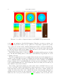
1
PISM, A PARALLEL ICE SHEET MODEL:
USER’S MANUAL
ED BUELER∗ , JED BROWN, AND NATHAN SHEMONSKI
Date: February 11, 2008. ∗ [email protected].
Based on PISM version “stable0.1” and PETSC release 2.3.3-p2.
Get PISM by Subversion:
svn co http://svn.gna.org/svn/pism/branches/stable0.1 pism.
2
PISM USER’S MANUAL
Copyright (C) 2004–2008 Ed Bueler and Jed Brown and Nathan Shemonski
This file is part of PISM.
PISM is free software; you can redistribute it and/or modify it under the terms of
the GNU General Public License as published by the Free Software Foundation;
either version 2 of the License, or (at your option) any later version.
PISM is distributed in the hope that it will be useful, but WITHOUT ANY
WARRANTY; without even the implied warranty of MERCHANTABILITY or
FITNESS FOR A PARTICULAR PURPOSE. See the GNU General Public License for more details.
You should have received a copy of the GNU General Public License along with
PISM; see pism/COPYING; if not, write to the Free Software Foundation, Inc., 51
Franklin St, Fifth Floor, Boston, MA 02110-1301 USA
Acknowledgements
The NASA Cryospheric Sciences Program supported this research with grant NAG5-11371.
Dave Covey and Don Bahls have been the best possible system administrators for the machines
on which we have developed PISM. Thanks to Martin Truffer, Kent Overstreet, Art Mahoney,
Ryan Woodard, and other PISM users for helpful comments and questions on PISM, the installation process, and this Manual.
PISM USER’S MANUAL
3
Contents
1. Introduction
2. Installation
3. Getting started
3.1. Running an EISMINT simplified geometry experiment
3.2. PISM’s standard output
3.3. Visualizing the results
3.4. Evolution runs versus “diagnostic” runs
4. Ice dynamics in PISM
4.1. Two different shallow models of ice flow
4.2. Tradition: Evolutionary SIA ice sheet versus diagnostic SSA ice shelf modeling
4.3. The floating-grounded mask
4.4. Schoof’s plastic till free boundary problem for ice streams
5. Initialization and “bootstrapping”
5.1. Initialization from a saved model state
5.2. Bootstrapping
5.3. Input file formats
6. More on usage
6.1. The PISM coordinate system and grid
6.2. Regridding
6.3. Understanding and controlling adaptive time-stepping
6.4. Using signals to control a running PISM model
6.5. Using the positive degree-day model
7. Verification
8. Simplified geometry experiments
8.1. Historical note
8.2. EISMINT II in PISM
9. Example: Modeling the Greenland ice sheet
10. Example: Validating PISM as a flow model for the Ross ice shelf
11. Inside PISM: overviews of continuum models and numerical schemes
11.1. The continuum models in PISM
11.2. The numerical schemes in PISM
References
Appendix A. PISM command line options
Appendix B. PETSC command line options (for PISM users)
Appendix C. PISM viewers: Graphical and Matlab
Appendix D. Python scripts for PISM modeling
4
5
10
10
11
13
13
15
15
16
16
17
19
19
19
20
21
21
22
23
23
25
28
34
34
34
37
48
54
54
54
56
59
68
69
72
4
PISM USER’S MANUAL
1. Introduction
Welcome to PISM!
This User’s Manual describes how to download the PISM source code and install PISM. It
describes how to run it for certain simplified geometry situations. It illustrates how PISM’s
numerical codes are verified. It describes how to use PISM as a modest Greenland ice sheet
model or a modest Ross ice shelf model.
But that is all. Users who want to advance the science of ice sheets will need to go beyond
what is described here. For such users there are two additional documents to know about:
(1) The PISM Reference Manual (www.pism-docs.org/refman.pdf) describes the most
important pieces of the source code. It contains, or at least it is intended to contain,
the minimum documentation of the PISM source code parts in order to include all the
continuum models and numerical methods of PISM.
(2) The PISM (HTML) Source Code Browser gives a complete view of the class/object
structure of the source code. It can be generated from the source by starting in the
PISM directory and doing cd doc/ && make. Then use a web browser like Firefox to
view pism/doc/doxy/html/index.html.
The Reference Manual and the Source Code Browser were automatically generated by doxygen
(www.doxygen.org) from comments in the PISM source code. Thus they are not as user-friendly
as this User’s Manual.
WARNING: PISM is an ongoing project. Ice sheet modeling is complicated and not
mature (in 2008, anyway). Please don’t trust the results of PISM or any other ice sheet
model without a fair amount of exploration. Also, please don’t expect all your questions
to be answered here. But do write to us with questions:
[email protected].
PISM USER’S MANUAL
5
2. Installation
Installing prerequisities.
1. You will need a UNIX system with internet access. A GNU/Linux environment will
be easiest but other UNIX versions have been used successfully. Package management
systems are useful for installing many of the tools below, but neither PISM itself nor
up-to-date PETSc distributions are currently available in the Debian repositories. You
will need Python and Subversion installed, but these are included in all current Linux
distributions. To use the (recommended) graphical output of PISM you will need an (X
Windows server.
2. As PISM is currently under rapid development, we distribute it only as compilable source
code. On the other hand, there are several software libraries needed by PISM. Therefore
the “header files” for these libraries are required for building PISM. In particular this
means that the “developer’s versions” of the libraries are needed if the libraries are downloaded from package repositories like Debian. (In summary, xorg-dev, netcdfg-dev,
libgsl0-dev, and fftw3-dev are the Debian packages we—the PISM developers—have
used in compiling and linking PISM.)
3. PISM uses NetCDF (= network Common Data Form) for an input and output file
format. If it is not already present, install it using the instructions at the webpage or
using a package management system.
4. PISM uses the GSL (= GNU Scientific Library) for certain numerical calculations and
special functions. If it is not already present, install it using the instructions at the
webpage or using a package management system.
5. PISM optionally uses the “FFTW” library (FFTW = Fastest Fourier Transform in the
West) in approximating the deformation of the solid earth under ice loads [10]. If you
want the functionality of this earth model, which is coupled to the ice flow and which
we recommend, install FFTW or check that it is installed already. If FFTW is not
installed, however, turn off PISM’s attempt to build with it by setting the environment
variable WITH_FFTW=0. If this library is absent, all of PISM will work except for the bed
deformation model described in the paper [10].
6. You will need a version of MPI (= Message Passing Interface). Your system may have an
existing MPI installation, in which case the path to the MPI directory will be used when
installing PETSc below. Otherwise we recommend that you allow PETSc to download
MPICH2 as part of the PETSc configure process (next). In either case, once MPI is
installed, you will want to add the MPI bin directory to your path so that you can
invoke MPI using the mpiexec or mpirun command. For example, you can add it with
the statement
export PATH=/home/user/mympi/bin:$PATH
(for bash shell)
or
setenv PATH /home/user/mympi/bin:$PATH
(for csh or tcsh shell).
Such a statement can, of course, appear in your .bashrc, .profile, or .cshrc file so
that there is no need to retype it each time you use MPI.
6
PISM USER’S MANUAL
From now on this manual will assume use of bash.
7. PISM uses PETSc (= Portable Extensible Toolkit for Scientific computation). As mentions of this library will occur frequently in this manual, note “PETSc” is pronounced
“pet-see”. Download the PETSc source by grabbing the current gzipped tarball at
www-unix.mcs.anl.gov/petsc/petsc-as/download/index.html
PISM requires a version of PETSc which is 2.3.3-p2 or later.1 The “lite” form of PETSc
is fine if you are willing to depend on an internet connection for accessing the PETSc
documentation.
You should configure and build PETSc essentially as described on the PETSc installation page, but it might be best to read the following comments on the PETSc configure
and build process first:
(i) Untar in your preferred location, but note PETSc should not be configured (next)
using root privileges. Note that you will need to define the environment variable
PETSC_DIR before configuring PETSc (next). For instance, once you have entered
the PETSc directory just untarred, export PETSC_DIR= 8 pwd8 . (Note the use of the
backprime (accent-grave) character, and not the single apostrophe ’.)
(ii) When you run the configure script in the PETSc directory, the following options
are recommended; note PISM uses shared libraries by default:
$ export PETSC_ARCH=linux-gnu-cxx
$ ./config/configure.py --with-shared --with-c-support \
--with-clanguage=cxx --with-debugging=no
Turning off the inclusion of the debugging symbols gives a significant speed improvement.
Note that there is no PISM use of Fortran, and that it is sometimes convenient to
have PETSc grab a local copy of BLAS and LAPACK rather than using the systemwide version. So one may add “--with-fortran=0 --download-c-blas-lapack=1”
to the other configure options.
(iii) If there is an existing MPI installation, for example at /home/user/mympi/, one
can point PETSc to it by adding the option --with-mpi-dir=/home/user/mympi/.
The path used in this option must have MPI executables mpicxx and mpicc, and
either mpiexec or mpirun, in subdirectory bin/ and MPI library files in subdirectory
lib/.
(iv) On the other hand, it seems common that one needs to tell PETSc to download MPI
into a place it understands, even if there is an existing MPI. If you get messages
suggesting that PETSc cannot configure using your existing MPI, you might try
configure.py with option --download-mpich=1.
(v) Configuration of PETSc for a batch system requires special procedures described at
the PETSc documentation site. One starts with a configure option --with-batch=1.
See the “Installing on machine requiring cross compiler or a job scheduler” section
of the PETSc installation page.
1
A Debian package for PETSc may exist, but it should only be used if it is version 2.3.3-p2 or later.
PISM USER’S MANUAL
7
(vi) Configuring PETSc takes many minutes even when everything goes smoothly. Note
that a previously installed PETSc can be reconfigured with a new PETSC_ARCH if
necessary.
(vii) After configure.py finishes, you will need to make all test in the PETSc directory and watch the result. If the X Windows system is functional some example
viewers will appear; as noted you will need the X header files for this to work.
(viii) Finally, you will want to set the PETSC_DIR and the PETSC_ARCH environment variables in your .profile or .bashrc file. Also remember to add the MPI bin directory to your PATH. For instance, if you used the option --download-mpich=1
in the PETSc configure, the MPI bin directory will have a path like $PETSC_DIR/
externalpackages/mpich2-1.0.4p1/$PETSC_ARCH/bin/. Therefore the lines
export PETSC_DIR=/home/user/petsc-2.3.3-p2/
export PETSC_ARCH=linux-gnu-cxx
export PATH=$PETSC_DIR/externalpackages/mpich2-1.0.4p1/$PETSC_ARCH/bin/:$PATH
could appear in one of those files.
See Table 1 for a summary of the dependencies on external libraries, including those mentioned
so far.
Installing PISM itself. At this point you have configured the environment which PISM needs.
You are ready to build PISM itself, which is a much quicker procedure!
6. Get the source for the stable branch of PISM using the Subversion version control system:
svn co http://svn.gna.org/svn/pism/branches/stable0.1 pism
A directory called “pism/” will be created. Note that in the future when you enter that
directory, svn update will update to the latest revision of PISM.2
7. Build PISM:3
cd pism
make
make install
Note that the “make install” puts executables, including pismd, pismr, pismv, and
pisms, in the pism/bin/ subdirectory and cleans up the junk from the build process.
“make install” does not require root permission.
8. PISM executables can be run most easily by adding the directories pism/bin/ and
pism/test/ to your PATH. The former directory contains the major PISM executables
while the latter contains several useful scripts. For instance, this command can be done
in the bash shell or in your .bashrc file:
export PATH=/home/user/pism/bin/:/home/user/pism/test/:$PATH
Quick tests of the installation. You are done with installation at this point. The next few items
are recommended as they allow you to observe that PISM is functioning correctly.
2Of course, after svn update you will make and make install to recompile and relink PISM.
3Please report any problems you meet at this build stage by sending us the output: [email protected].
8
PISM USER’S MANUAL
10. Try a serial verification run of PISM:
pismv -test G -y 100
If you see some output and a final Writing model state to file ’verify.nc’ ... done
then PISM completed successfully. Note that at the end of this run you get measurements of the difference between the numerical result and the exact solution [9].
11. Try the MPI four processor version of the above run:
mpiexec -n 4 pismv -test G -y 100
This should work even if there is only one actual processor on your machine, in which
case MPI will run multiple processes on the one processor, naturally. The reported
errors should be very nearly the same as the serial run above, but the results should
appear faster (if there really are four processors)!
12. Try a verification run on a finer vertical grid while watching the diagnostic views which
use Xwindows:
pismv -test G -Mz 201 -y 2000 -d HTc
When using such diagnostic views and mpiexec the additional final option -display :0
is sometimes required to enable MPI to use Xwindows:
mpiexec -n 2 pismv -test G -Mz 201 -y 2000 -d HTc -display :0
13. Run a verification test of the ice stream code:
pismv -test I -Mx 5 -My 401 -verbose
This runs a rather different part of the PISM code and then compares the numerical
result to the exact solution appearing in [62].
14. Run a Python script for a basic suite of verifications:
verifynow.py
or, on an N processor machine,
verifynow.py -n N
If you would like us to confirm that PISM is working as expected please save the one
page or so of output from this script and send it to us ([email protected]). See section 7
for more on PISM verification.
At this stage you can do the EISMINT II simplified geometry experiments (section 8) and
run many verification tests (section 7) without further downloads. Section 9 is an example of
using PISM to model the Greenland ice sheet using freely-downloadable data. Similarly one can
model the Ross ice shelf using free data as described in section 10.
Setting up PISM to model real ice sheets will frequently require techniques not be covered in
this manual. At the minimum, the user will need to convert ice sheet data to NetCDF format
so that it can be read by PISM. Actual modeling may also require the writing of additional
source code; see the Reference Manual for a description of the source code for PISM. Use of
PISM for real ice sheet modeling is something we welcome questions about, and will attempt
to help with, but we will not pretend it is routine. See the PISM Documentation web-page
www.pism-docs.org for links to additional documentation.
A final reminder with respect to installation: Let’s assume you have checked out a copy
of PISM using Subversion, as in step 6 above. You can update your copy of PISM to the
PISM USER’S MANUAL
9
latest version by svn update in the pism/ directory. After doing so you will want to make and
make install in order to rebuild the PISM executables using the updated source code files.
Have fun!
Table 1. Dependencies for PISM, listed alphabetically. These are needed to
build a fully-functional PISM from source and to do all the examples in the
manual.
Library
/Program
FFTW
Site
Required?
Comment
www.fftw.org
recommended
if not present set
WITH_FFTW=0 for PISM build
GSL
Matlab
www.gnu.org/software/gsl
www.mathworks.com
required
recommended
MPI
NetCDF
numpy
www-unix.mcs.anl.gov/mpi
required
www.unidata.ucar.edu/software/netcdf required
numpy.scipy.org
recommended
PETSc
Python
pycdf
www-unix.mcs.anl.gov/petsc
python.org
pysclint.sourceforge.net/pycdf
required
required
recommended
Subversion
subversion.tigris.org
required
only used for alternate
display of results
used in Python scripts
in sections 9 and 10
version ≥ 2.3.3-p2
used in Python scripts
in sections 9 and 10
Table 2. Additional dependencies for PISM needed only for serious developers
of PISM , listed alphabetically.
Library
/Program
LATEX
doxygen
ruby
Site
Comment
www.latex-project.org only used for rebuilding manuals (both this User’s Manual
and the Reference Manual) from source
www.doxygen.org
only used for rebuilding the Reference Manual and the
Source Code Browser from the source code files
www.ruby-lang.org
only used when changing the NetCDF format
for PISM output files
10
PISM USER’S MANUAL
3. Getting started
3.1. Running an EISMINT simplified geometry experiment. PISM’s purpose is the
simulation of actual ice sheets. But actual ice sheet simulations require actual data.4 For
now, in order to avoid issues of data formats and data flaws in a first use of PISM, this section describes how to use PISM for experiment F in the “EISMINT II” simplified-geometry,
thermomechanically-coupled ice sheet model intercomparison [51]. In this experiment one models an angularly-symmetric shallow, grounded ice sheet on a flat bed with relatively cold surface
temperatures.
In EISMINT II the prescribed grid has 60 subintervals in each direction, with each subinterval
of length 25km. Thus the total width of the computational box is 1500 km in both x and y
directions. However, PISM always allows choice of the grid in all three dimensions. A runtime
option chooses the number of grid points in each direction; note that the number of points is
one greater than the number of subintervals (grid spaces). The vertical grid is not prescribed in
EISMINT II. For a demonstration we choose this standard 25km grid in the horizontal and use
201 grid points in the vertical for a 25 m (equally-spaced) grid. (Note that the computational
box is 5000 m high by default for EISMINT II experiment A in PISM.) Experiment A starts
with zero ice, but the center thickness of the ice sheet grows to a peak near 5000 m before
decaying to its equilibrium center thickness of about ??? m. All EISMINT II runs are for
200,000 model years. Here we start with a short 2000 year run for a quicker illustration. The
executable is “pisms”, for the “simplifed geometry mode” of PISM:
$ pisms -eisII A -Mx 61 -My 61 -Mz 201 -y 2000
PISMS (simplified geometry mode)
setting parameters for EISMINT II experiment A ...
initializing EISMINT II experiment A ...
[computational box for ice: ( 1500.00 km) x ( 1500.00 km) x ( 5000.00 m)]
[grid cell dims (equal dz): (
25.00 km) x (
25.00 km) x (
25.00 m)]
running EISMINT II experiment A ...
%ybp SIA SSA # vgatdh Nr +STEP
P
YEAR:
ivol
iarea
meltf
thick0
temp0
U
years 10^6_km^3 10^6_km^2 (none)
m
K
$$$$
$$$$$ $$
S
0.00000: 0.00000 0.0000
0.0000
0.000 238.1500
$$$ SIA
v$at$h 0m +60.00000
S
60.00000: 0.01704 0.6281
0.0000
30.000 238.1500
. . .
$$$ SIA
v$at$h 0e +20.00000
S
2000.00000: 0.56790 0.6306
0.0000
1000.000 243.7518
done with run ...
Writing model state to file ‘simp_exper.nc’ ... done.
This should have taken less than one minute.
4Actual
ice sheet and ice shelf data are freely available as part of the EISMINT intercomparison efforts. Section
9 is a tutorial on the use of PISM as a Greenland ice sheet evolution model and section 10 is a tutorial on PISM
as an Ross ice shelf diagnosity model using the EISMINT data sets.
PISM USER’S MANUAL
11
In a moment we will address the standard output information provided by PISM, as shown
above, but for now we simply illustrate how to restart and complete the 200,000 year run. We see
that the model state was stored in a NetCDF file with the pisms default name “simp_exper.nc”.
The next run will use a “-o” option to name the output file. Also, the above was a single
processor run, but let’s suppose we have a four processor machine. (The following should also
work fine on a single processor machine but there is no speed-up, naturally.) Let’s also run
things in the background so we can continue to experiment:
$ mpiexec -n 4 pisms -eisII A -if simp_exper.nc -tempskip 5 -y 198000 \
-o eisIIA200k >> eisIIA.out &
This run will take at least four processor-hours. It generates a NetCDF file eisIIA200k.nc
at the end. The standard output in eisIIA.out can be tracked as the job is running in the
background using less, for instance; top is a Linux tool to watch CPU and memory usage
during the run.
To get the model state in the midst of a PISM run, send all running pisms processes
(that’s the executable in this case) a signal which causes PISM to write out the model state:
pkill -USR1 pisms. The PISM model state is then saved in a NetCDF file with name pism-year .nc,
using the year at that time step. On the other hand, terminatating the run with pkill -TERM pisms
will will cause PISM to stop, but only after saving the model state using the -o specified name
(though it will not hold the result of the completed run). See subsection 6.4 for a more complete
description of how PISM catches signals.
While the four processor pisms run continues in the background, let’s view the model state
during a few time steps by restarting from the saved 2000 year state. We use PISM’s “diagnostic
viewers”, which requires X Windows:
$ pisms -eisII A -if simp_exper.nc -y 1000 -d HTt
Three figures should appear and be refreshed at each time step. One figure is a map-plane
view of thickness, another is a map-plane view of the basal temperature in Kelvin, and third
there is a graph of height above the bed versus temperature. When the full 200,000 year run
finishes, one may watch its evolving state, including the ice flow speed, by
pisms -eisII A -if eisIIA200k.nc -d HTc
for example. Figure 1 will appear.
3.2. PISM’s standard output. As illustrated already, at each time step PISM shows a summary of the model state using a flags and a few numbers. The format of the summary is
suggested by the three mysterious lines near the beginning of the run:
%ybp SIA SSA # vatdh Nr +STEP
P
YEAR:
ivol
iarea
meltf
U
years 10^6_km^3 10^6_km^2 (none)
thick0
m
temp0
K
The first line gives flags which indicate which physical models ran at the given time step, so it
shows which quantities were updated. A dollar sign “$” appears if a given model did not run.
From the left the first three positions are: y for basal yield stress model, b for bed deformation
model, and p for plastic till yield stress. Then either “SIA” or “SSA” appear, or both, and the
if the “SSA” flag is present it is followed by the number of iterations of the SSA model. (See
12
PISM USER’S MANUAL
Figure 1. Screenshot of diagnostic figures for an EISMINT II experiment A run.
section 4 for an explanation of the SIA/SSA language.) Then there are six more positions: v for
velocity updates (by SIA or SSA), a for age equation, t for temperature equation, d for positive
degree day model, and h for mass continuity (which updates surface elevation and thickness).
Finally an integer N appears (it is most frequently zero), and another single character flag
r. Then the time step itself is given (STEP). These all related to the decisions of the adaptive
time-stepping scheme; described in subsection 6.3.
The next line starting with “P” is the prototype for the summary which appears at each time
step. The third line starting with “U” is the units for this summary; it appears just once at the
beginning of the run.
The time step STEP and the model year YEAR, which is the first entry in the summary line, are
in units of years. The 200k year run above illustrates how the time-stepping in PISM adapts in
order to maintain stability for its (mostly) explicit methods. At the beginning of the EISMINT
II run, for instance, the ice has small thickness so the time step is 60 years, simply because that
is the default maximum time step. Later in that run, after about 5000 years, the time step is
made smaller because the flow is faster.
The next three entries in the summary report the volume of the ice in 106 km3 , the area covered
by the ice in 106 km2 , and the basal melt fraction, that is, the fraction of the ice area where the
basal temperature is at the pressure-melting temperature. The next two columns “thick0” and
“temp0” are values at the center of the computational domain of the map plane, namely the ice
thickness in meters and the absolute temperature of the ice at its base, in Kelvin. These five
numbers are the ones reported in the tables in [51]. The summary of the model state can be
PISM USER’S MANUAL
13
made more verbose by using the option -verbose. For more on the EISMINT II experiments
see section 8.
3.3. Visualizing the results. There are four basic methods for visualizing the various quantities in PISM, namely
1)
2)
3)
4)
runtime viewers under Xwindows,
visualizing model state NetCDF files from the end of a run,
using Matlab to view individual variables at the end of a run, and
turning the PISM standard output (above) into time series and viewing graphs of those.
As shown by the “-d HTt” option illustrated above, runtime viewers can be specified by
options of the form -d letters or -dbig letters. The latter option shows larger windows but is
otherwise identical. See Appendix C for the possible single letter names of each runtime viewer.
These viewers are updated at each step. As they work under Xwindows, MPI must be told
how to send data to the window, so PISM options are usually followed by “-display :0” when
PISM is run under MPI and runtime viewers are desired.
The format is limited by the style of PETSc viewers, but these viewers often suffice for
visualizing an ongoing PISM run. Note that some diagnostic viewers show slices of threedimensional quantities in slices parallel to the bed. They are controlled by the option -kd.
Those which show “soundings” are controlled by the options -id, -jd; see Appendices A and
C.
Regarding method 2), when a PISM run is finished the state of the model is output in NetCDF
format. The name can be specified by the option -o, so -o foo writes the NetCDF file foo.nc.
NetCDF files can be viewed or modified with a variety of tools, some of which are mentioned in
table 3. The PISM developers find ncview to be the fastest way to look at PISM output files,
but ncview is not as sophisticated as many other scientific visualization programs which handle
NetCDF files, such as IDV.
Regarding method 3), the user can add options of the form -mato foo and -matv letters to
save certain variables in Matlab-readable ASCII form at the end of the run. In particular, the
saved file foo.m is a standard Matlab script. The single letter arguments to -d and -matv are
generally the same. See Appendix C.
Appendix D describes a Python script series.py which can post-process the standard output
from a PISM run into a NetCDF file with the time series for the quantities listed in PISM
standard output.
3.4. Evolution runs versus “diagnostic” runs. The main goal of a numerical ice sheet
model like PISM is to be a dynamical system which evolves over time as similarly as possible to
the modeled ice sheet. Such a goal assumes one starts with the right initial conditions and that
one has the right climate and other inputs at each time step. Underlying an ice sheet model like
PISM are evolution-in-time partial differential equations, and the obvious mode for a numerical
ice sheet model is to take small time steps in approximating these differential equations; “small
time steps” could mean several model years, of course. We will describe this usual time-stepping
behavior as an “evolution run.”
14
PISM USER’S MANUAL
Table 3. Tools for viewing and modifying NetCDF files.
Tool
Site
Function
ncdump
included with any NetCDF distribution
dump as text file
ncview
http://meteora.ucsd.edu/~pierce/ncview_home_page.html quick graphical view
ncBrowse
www.epic.noaa.gov/java/ncBrowse/
quick graphical view
IDV
www.unidata.ucar.edu/software/idv/
more complete visualization
NCO = NetCDF nco.sourceforge.net/
sophisticated manipulations
Operators
at command line
See www.unidata.ucar.edu/software/netcdf/docs/software.html for additional tools.
Much of ice sheet, stream, and shelf modeling, however, requires only “diagnostic” solution
of the partial differential equations which determine the velocity field. These are the balance
of momentum equations for a slowly flowing fluid, and shallow approximations thereof [17]. In
a diagnostic computation the temperature field and certain basal conditions, such as the yield
stress of the till for instance, are held fixed. The goal of a “diagnostic run” is to compute the
velocity field; this will be the definition used from now on in this manual.
Note that, as explained in the next section, the “shallow ice approximation” (SIA), on which
the EISMINT II experiments are based, is only one of two forms of the balance of momentum
equations solved by PISM. The other is the “shallow shelf approximation” (SSA). Both of these
models can be solved in either evolution or diagnostic mode.
As a diagnostic example, using the quantities already computed in this section, try
pismd -if eisIIA200k.nc -o eisIIA200k_diag
The result of this command is a NetCDF file eisIIA200k_diag.nc which contains the full
three-dimensional velocity field in the scalar NetCDF variables uvel, vvel, and wvel.
The velocity field saved by pismd is the one which would be computed at the next time step
in an evolution run. That is, if we also run
pisms -eisII A -if eisIIA200k.nc -y 0.001 -o eisIIA200k_plus
then the horizontal velocity field computed in this single time step run is the same as that saved
in eisIIA200k_diag.nc.5
This diagnostic mode is most frequently associated to the modeling of ice shelves and ice
streams. Subsection 10 describes the use of pismd in modeling the Ross ice shelf [42].
Note that the NetCDF model state saved by PISM at the end of an evolution run does not,
by default, contain the three-dimensional velocity field. Instead, it contains just the variables
which are needed to restart the run, especially the ice geometry and temperature field. One
can also force PISM to save the full velocity field at the end of a time-stepping run using the
option -f3d. The diagnostic executable pismd saves the full three-dimensional velocity field by
default. Either way, saving the full velocity field roughly doubles the size of the saved NetCDF
file.
5For
this example, one can use a NetCDF Operator to check that the two saved NetCDF files contain essentially
the same vertically-averaged horizontal velocity field; just do ncdiff -v cbar . . .
PISM USER’S MANUAL
15
4. Ice dynamics in PISM
4.1. Two different shallow models of ice flow. PISM can numerically solve two significantly
different sets of equations which determine the velocity field within the ice. In both cases the
geometry of the ice, the temperature field within the ice, and the stress condition at the base
of the ice are included into balance of momentum equations to determine the flow. But there
are two different versions of the balance of momentum equations:
• the shallow ice approximation (SIA) [29], which describes ice flowing by shear in planes
parallel to the geoid, with such shearing a local function of the driving stresses of classical
glaciology [47], and
• the shallow shelf approximation (SSA) [65], which describes a membrane-type flow with
the ice floating or sliding over a weak base [43, 41, 62].
PISM numerically solves both the SIA and SSA equations in parallel. Time-stepping solutions
of the mass continuity equation are possible for both models.
The SIA equations are, as a rule, easier and quicker to numerically solve than the SSA. The
SIA equations are also easier to parallelize. They can confidently be applied to those grounded
parts of ice sheets for which the basal ice is frozen to the bedrock and the bed topography
is relatively slowly-varying the map-plane [17]. We recommend only solving the SIA with a
nonsliding base because the addition of a “sliding law” which switches on at the pressure-melting
temperature tends to have deeply undesirable numerical consequences.
The SSA equations can confidently be applied to large floating ice shelves because such shelves
have small depth-to-width ratio and because there is no shear stress at the base of the floating
ice [43, 44].
Ice sheets have faster-flowing grounded parts, however. These are usually called “ice streams”
or “outlet glaciers”. Such features appear at the margin of, and even well into the interior of,
the Greenland [37] and Antarctic [2] ice sheets. Describing these faster-flowing grounded parts
of ice sheets requires something more than the non-sliding base SIA. Ultimately one might use
the full Stokes equations which represent the balance of all tensor components [17], but there is
still the issue of the appropriate sliding boundary condtion. Similarly one might use a “higherorder” but still shallow stress balance [5, 49], but again a proper choice of boundary condition
is equally important.
Though they apply with greatest confidence to ice shelves, one may apply the SSA equations
with additional basal resistance terms to grounded ice. This was justified in the context of the
Siple Coast ice streams of Antarctica by MacAyeal [41, 27] using a linearly-viscous model for the
underlying till. On the other hand, a free boundary problem with essentially the same (SSA)
balance equations is the Schoof [62] model of ice streams. In Schoof’s model ice streams emerge
in those parts of the ice sheet where there is plastic till failure; see also [63].
These SSA equations with additional basal resistance are the models PISM uses to describe
faster-flowing grounded ice. The SSA version of the balance of momentum equations with
linearly-viscous till are solved as a fixed-boundary problem (at a particular time step), and thus
the locations and extent of ice streams must be determined by some other criterion. For the
SSA version of the balance of momentum equations with plastic till, as noted, the locations of
16
PISM USER’S MANUAL
ice streams is determined as part of the free boundary problem. In fact we believe that the
plastic till SSA of Schoof should be regarded as the best currently implementable “sliding law”
for the SIA.
As noted, both the SIA and SSA models are shallow approximations. That is, the partial differential equations in these two approximations come by (different) small-parameter arguments,
based on a small depth-to-width ratio, from the Stokes equations of a non-Newtonian fluid. For
this small-parameter argument in the SIA case see [17]. For the corresponding SSA argument,
see the appendices of [62].6
By default, PISM does not numerically solve the SSA when using the executables pismr,
pismd, or pisms. The user must add the flag -ssa. The rules for verifying the SSA balance of
momentum equations using the verification executable pismv are addressed in section 7.
4.2. Tradition: Evolutionary SIA ice sheet versus diagnostic SSA ice shelf modeling.
Sections 9 and 10 illustrate the two traditional ice flow models, namely a time-stepping SIA-only
model for the Greenland ice sheet and a diagnostic SSA model for the Ross ice shelf.
Note Tests A, B, C, D, E, F, G, H, and L in the verification suite are evolutionary runs using
only the SIA. Tests I and J are diagnostic calculations using the SSA. See section 7.
All of the “EISMINT II” experiments documented in section 8 are evolutionary runs using
only the SIA.
4.3. The floating-grounded mask. The most basic decision about ice dynamics made internally by PISM is to apply the “floatation criterion” to determine whether the ice is floating on
the ocean or not.7 In an evolution run this decision is made at each time step and the result is
stored in the mask.
The possible values of the mask are given in Table 4. The mask does not by itself determine ice dynamics. For instance, when ice is floating (either value MASK_FLOATING or
MASK_FLOATING_OCEAN0) the usual choice for ice dynamics is SSA, but the user can choose
not to apply that model by leaving off the option -ssa.
Table 4. The PISM mask along with user options determines the dynamical
model. This description gives only an incomplete view . . .
Value
1
2
3
7
Name
MASK_SHEET
MASK_DRAGGING
MASK_FLOATING
MASK_FLOATING_OCEAN0
Meaning
ice is grounded (and the SIA is usually applied)
ice is grounded (and the SSA is applied if option -ssa is given)
ice is floating (and the SSA is applied if option -ssa is given)
same as MASK_FLOATING, but the grid point was ice free
ocean at initialization of the model by -bif;
ice with MASK_FLOATING_OCEAN0 will calve off
if option -ocean_kill is given.
6The references are, of course, the right place to examine the continuum equations and their physical motiva-
tion. This manual avoids serious discussion of continuum ice dynamics.
7See [65] for a definition and discussion of this criterion.
PISM USER’S MANUAL
17
The remainder of this section gives an incomplete view, at best, of the dynamics in PISM.
See sections 9 and 10 for examples which suggest the traditional modes of ice sheet and shelf
modeling. Times they are a’changing, however, and PISM is too . . .
4.4. Schoof ’s plastic till free boundary problem for ice streams. In [63] C. Schoof
proposes a model for plastic failure of the basal till under flowing ice, and in [62] he recognizes
this as a free boundary problem for the SSA. The result is a model for emergent ice streams
within a larger ice sheet and ice shelf system. It explains the existence of ice streams by
a combination of the plastic failure of the till and the SSA approximation of the balance of
momentum.
PISM implements Schoof’s model (among others, of course). The user gives the options
-ssa -plastic to turn it on. All grounded points are immediately marked as SSA (i.e. as
MASK_DRAGGING). At these points a yield stress is computed from the amount of stored basal
water, a thermodynamic quantity, and from a (generally) spatially-varying till strength. See
the description of option -plastic in Appendix A for a detailed description of the yield stress
computation; see also the PISM Reference Manual.
A plastic till modification of EISMINT II experiment I. To demonstrate the Schoof model we
describe an example based on EISMINT II experiment I.
The original EISMINT experiment I is only documented in [50], but not, however, in the published intercomparison [51]. (That reference says that for experiment I results were “straightforward . . . with little variability between groups” but also that the results were “difficult to
interpret”.) Note that Section 8 describes using PISM to perform all the EISMINT II experiments documented in [50], including the original experiment I. Experiment I is identical to
experiment A except for having “trough” bed topography.
As specified, the original experiment I has nothing to do with the SSA equations or plastic till
failure, and indeed there is no basal motion at all. However, we use it to build an ice sheet which
“ought” to have an ice stream, that is, along the trough. The script test/eis2plastic.sh gives
a sequence which starts with the plain experiment I on a standard EISMINT II grid and builds
an ice sheet modeled by SIA. It then turns on the plastic till SSA and superposes the velocity
fields.
This plastic till modified experiment is for now only documented in [8], in preparation.
Test I is an exact solution. Test I in the verification suite is an instance of the exact solution
to the plastic till SSA published in [62]. It is a single diagnostic computation of the velocity of
a highly-simplified ice stream. Here is an example run with some viewers:
pismv -test I -Mx 5 -My 121 -d ncqu
The boundary conditions are a uniform slab of ice on a bed with constant slope, but with a
central minimum in a pre-specified distribution of till yield stress. There is zero yield stress
at the very center. Thus the center of the slab slides. The ice flows under the SSA equations,
because of the plastic failure, while at the margins the base of the ice does not slide. Thus
we have an ice stream. The velocity only varies in the cross-slope direction. PISM’s job is to
compute the width and speed of the ice stream, “knowing” only the ice thickness, bed slope,
and yield stress distribution. In this case we have the exact solution with which to compare the
18
PISM USER’S MANUAL
numerically-computed velocities. This test, and convergence of PISM’s numerical solution of it
under grid refinement, are addressed in section 7.
PISM USER’S MANUAL
19
5. Initialization and “bootstrapping”
5.1. Initialization from a saved model state. This phrase has a simple meaning in PISM.
If a previous PISM run has saved a NetCDF file using “-o” then that file will contain complete
initial conditions for continuing the run. The output file from the last run can be loaded with
“-if”, as in this example:
$ pisms -eisII A -y 100 -o foo
$ pisms -eisII A -if foo.nc -y 100 bar
Note that simplified-geometry experiments (section 8) and verification tests (section 7) do
not need input files at all. They initialize from formulas in the source code, but they can be
continued from saved model states using -if. As in the above example, however, specifying
which simplified geometry experiment (or verification test) is in use is necessary. For instance,
if the second line above is replaced by
$ pisms -if foo.nc -y 100 bar
then an error is generated.
5.2. Bootstrapping. “Bootstrapping” PISM means giving it less than complete data, and
letting it fill in the needed data according to heuristics. These heuristics are applied before the
first time step is taken, so they are part of an initialization process. Bootstrapping uses the
option “-bif”.
In some sense, bootstrapping is unprincipled inverse modelling. It is possible, for instance, to
estimate the sliding state of the base of the ice through inverse models ([38] is an example8). It
is also possible to use observed “isochrones” from ice-penetrating radar to estimate the velocity
of ice [15].
Instead, however, most ice sheet modeling (using forward models like PISM) would do something like this to get “reasonable” temperature and velocity fields within the ice:
1) start only with observable quantities like surface elevation, ice thickness, and ice surface
temperature,
2) “bootstrap” as described in this section, to fill in temperatures at depth and give a
preliminary estimate of the basal sliding condition and the three-dimensional velocity
field, and
3) either do a long run holding the current geometry and surface temperature steady, to
evolve toward a “more physical” steady state which will have compatible temperature
field, velocities, and age field,
4) or do a long run using an additional spatially-imprecise historical record from an ice
core or a sea bed core (or both), to add apply forcing to the surface temperature or
sea level (for instance), but with the same functional result of filling in a temperature,
velocity, and age.
Subsection 9 does EISMINT-Greenland [55, 30] as an example of bootstrapping. That section
shows examples of long runs of both types (3) and (4).
8The
PISM authors are eager to work with principled (or at least, serious) inverse modelers. In particular,
we would like to inverse-model-derived basal shear stresses to constrain a PISM forward model which would use
both SIA and SSA models of ice flow.
20
PISM USER’S MANUAL
When using -bif you will usually have to specify the height of the computational box for the
ice with -Lz Z, and add option -Lbz Zb if you want a bedrock thermal layer. This additional
specification is natural: the data used in “bootstrapping” will usually be two-dimensional.
5.3. Input file formats. The NetCDF format of a PISM output model state file is described
by the CDL file
pism/src/netcdf/pism_state.cdl
The file used with “-if” must have this format, but this is no difficulty for the user, as it will
have been produced by a previous PISM run.
The allowed formats for a bootstrapping file are now relatively simple to describe. The
NetCDF dimensions t,x,y,z,zb and corresponding variables must be present and match the
choices in pism_state.cdl, or in a PISM output file. But any of the other two dimensional
variables (depending on t,x,y) may be missing, and for those missing values some heuristic will
be applied. All three dimensional variables (depending on t,x,y,z or t,x,y,z) will be ignored
in bootstrapping.
The heuristics themselves are, for now, only documented in the source code:
pism/src/base/iMbootstrap.cc
Also see the PISM Reference Manual. Serious modeling is likely to start with the default
bootstrapping method in iMbootstrap.cc, called by the option “-bif”, but then add additional
source code to add information. This additional source code is likely to be a derived class of
IceModel. The code in
pism/src/eismint/iceGRNModel.hh
and
pism/src/eismint/iceGRNModel.cc
is an example of such a derived class; it does EISMINT-Greenland, as noted. Its function is
fully documented in section 9.
PISM USER’S MANUAL
21
6. More on usage
6.1. The PISM coordinate system and grid. PISM does all simulations in a computational
box which is rectangular in the PISM coordinates.
The coordinate system has horizontal coordinates x, y and a vertical coordinate z. The z
coordinate is measured positive upward from the base of the ice and it is exactly opposite to
the vector of gravity. The surface z = 0 is the base of the ice, however, and thus is usually not
horizontal in the sense of being parallel to the geoid. The surface z = 0 is the base of the ice
both when the ice is grounded and when the ice is floating.
Bed topography is, of course, allowed. In fact, when the ice is grounded, the true physical
vertical coordinate z 0 , namely the coordinate measure relative to a reference geoid, is given by
z 0 = z + b(x, y) where b(x, y) is the bed topography. The surface z 0 = h(x, y) is the surface of
the ice. Thus in the grounded case the equation h(x, y) = H(x, y) + b(x, y) applies if H(x, y) is
the thickness of the ice.
In the floating case, the physical vertical coordinate is z 0 = z − (ρi /ρs )H(x, y) where ρi is
the density of ice and ρs the density of sea water. Again z = 0 is the base of the ice, which is
the surface z 0 = −(ρi /ρs )H(x, y). The surface of the ice is h(x, y) = (1 − ρi /ρs )H(x, y). All we
know about the bed elevations is that they are below the base of the ice when the ice is floating.
That is, the floatation criterion −(ρi /ρs )H(x, y) > b(x, y) applies.
The computational box can extend downward into the bedrock. As z = 0 is the base of
the ice, the bedrock corresponds to negative z values regardless of the sign of its true (i.e. z 0 )
elevation.
The extent of the computational box, along with its bedrock extension downward, is determined by four numbers Lx, Ly, Lz, and Lbz. The first two of these are half-widths and have
units of kilometers when set by options or displayed. The last two are vertical distances in the
ice and in the bedrock, respectively, and have units of meters. See the sketch in figure 2.
Figure 2. PISM’s computational box.
The extent of the computational box for the ice is directly controlled by the options -Lx, -Ly,
and -Lz as described in the Runtime options section. As noted -Lx and -Ly options should
include values in kilometers while -Lz should be in meters.
22
PISM USER’S MANUAL
The PISM grid covering the computational box is equally spaced in each of the three dimensions. Because of the bedrock extension, the grid of points is described by four numbers, namely
the number of grid points in the x direction, the number in the y direction, the number in the
z direction within the ice, and the number in the z direction within the bedrock. These are
specified by options -Mx, -My, -Mz, and -Mbz, respectively, as described in the Runtime options
section. The defaults for these four values are 61, 61, 31, and 1, respectively. Note that Mx, My,
Mz, and Mbz all indicate the number of grid points. Therefore the number of grid spaces are,
respectively, 60, 60, 30, and 0 (zero) in the default case. Note that the lowest grid point in a
column of ice, that is the one at z = 0, coincides with the highest grid point in the bedrock.
Also Mbz must always be at least one.
The distance Lbz is controlled by specifying the number Mbz of grid points in the bedrock,
noting that the vertical spacing dz is the same within the ice and within the bedrock. To avoid
conflicts, the distance Lbz cannot be set directly by the user. In particular, Lbz = dz (Mbz − 1)
while dz = Lz/(Mz − 1), and so the distance Lbz into the bedrock is determined by setting Lz,
Mz, and Mbz.
One is allowed to specify the grid when PISM is started without a pre-existing model state
(i.e. as stored in a NetCDF input file output by PISM). For instance, a shortened EISMINT II
experiment A [51] run, which will produce a convenient NetCDF file for our purposes here, is
$ pisms -eisII A -Mx 61 -My 61 -Mz 101 -y 5000 -o foo
If one initializes PISM from a saved model state then the input model state controls the parameters Mx, My, Mz, and Mbz. For instance, the command
$ pisms -eisII A -if foo.nc -Mz 201 -y 100
will give a warning that “user option -Mz ignored; value read from file foo.nc.” To
change the model grid one must explicitly “regrid”, as described next.
6.2. Regridding. It is common to want to interpolate a coarse grid model state onto a finer
grid or vice versa. For example, one might want to do the EISMINT II experiment as above,
producing foo.nc, but then interpolate both the ice thickness and the temperature onto a finer
grid. Speaking conceptually, the idea in PISM is that one starts over from the beginning of
EISMINT II experiment A on the finer grid, but one extracts the thickness and ice temperature
stored in the coarse grid file and interpolates onto the finer grid before proceeding with the
actual computation. The transfer from grid to grid is reasonably general—one can go from
coarse to fine or vice versa in each dimension x, y, z—but the transfer must always be done by
interpolation and never extrapolation. (An attempt to do the latter will always produce a PISM
error.)
Such “regridding” is done using the -regrid and -regrid_vars commands as in this example:
$ pisms -eisII A -Mx 101 -My 101 -Mz 201 -y 1000 \
-regrid foo.nc -regrid_vars HT -o bar
By specifying regridded variables “HT”, the ice thickness and temperature values from the old
grid are interpolated onto the new grid. Note that one doesn’t need to regrid the bed elevation,
which is set identically zero as part of the EISMINT II experiment A description, nor the ice
surface elevation, which is computed as the bed elevation plus the ice thickness at each time
step anyway.
PISM USER’S MANUAL
23
See table 5 for the regriddable variables.
A slightly different use of regridding occurs when “bootstrapping” as described in section 5
and illustrated by example in section 9.
Table 5. Regriddable variables. “.nc Name” gives the name of the variable in
a PISM output NetCDF file. Use -regrid var with given flag.
Flag
a
b
B
e
g
H
L
s
T
.nc Name
acab
topg
litho temp
age
bheatflx
thk
bwat
artm
temp
Variable
(net annual) accumulation
bed elevation
temperature in bedrock
age of the ice
geothermal flux
thickness
thickness of basal melt water
ice surface temperature
ice temperature
Comment
climate; usually not regridded
climate; usually not regridded
climate; usually not regridded
6.3. Understanding and controlling adaptive time-stepping. Recall that at each time
step the PISM standard output includes flags and a summary of the model state using a few
numbers.:
%ybp SIA SSA # vgatdh Nr
P
YEAR:
ivol
+STEP
iarea
meltf
thick0
temp0
Here we explain what ‘Nr’ and ‘STEP’in the flag line mean.
STEP is the time step just taken by PISM, in model years. This time step is determined
by a somewhat complicated adaptive mechanism. Note that PISM does each step explicitly
when numerically approximating mass conservation in the map-plane. This, and the modeling
of advection [9], requires and adaptive time-stepping scheme.
Note that most of the time ‘N’ in the flag line will be zero. The exception is when the option
-tempskip is used. If -tempskip M is used, then N will be at most M , and will countdown
the mass conservation steps when the adaptive scheme determines that a long temperature/age
evolution time step, relative to the diffusity controlled time step for mass conservation, would
be allowed. To see an example, do:
$ pismv -test G -Mx 141 -My 141 -Mz 51 -tempskip 4
Table 6 explains the meaning of the one character adaptive-timestepping flag ‘r’.
6.4. Using signals to control a running PISM model. Ice sheet model runs sometimes
take a long time and the state of the run needs checking. Sometimes they need to be stopped,
but with the possibility of restarting. PISM implements these behaviors using “signals” from
the POSIX standard. Such signals are included in Linux and most flavors of Unix. Table 7
below summarizes how PISM responds to signals.
24
PISM USER’S MANUAL
Table 6. Meaning of the adaptive time-stepping flag ‘r’ in standard output flag line.
Flag
c
d
e
f
m
t
u
Active adaptive constraint
3D CFL for temperature/age advection [9]
diffusivity for SIA mass conservation [9]
end of prescribed run time
-dt_force set; generally option -dt_force, which overrides the adaptive scheme,
should not be used
maximum allowed ∆t applies; set with -max_dt
maximum ∆t was temporarily set by a derived class; e.g. see effect of deliverables
-timen in pisms -ismip H \timen
2D CFL for mass conservation in SSA regions (where mass conservation is upwinded)
Here is an example. Suppose we start a long verification run in the background, with standard
out redirected into a file:
pismv -test G -Mz 101 -y 1e6 -o testGmillion >> log.txt &
This run gets a Unix process id (“pid”); we will need that number. (One can get the pid by
using the ps or pgrep utilities.)
If we want to observe the run without stopping it we send the USR1 signal:
kill -USR1 8920
where “8920” happened to be the pid of the running PISM process. It happens that we caught
the run at year 31871.5 or so because a NetCDF file pism-31871.495239.nc is produced. This
intermediate state file can be viewed by ncview pism-31871.495239.nc. Note also that in the
standard out log file log.txt the line
...
Caught signal SIGUSR1: Writing intermediate file ‘pism-31871.495239.nc’.
...
appears around time step (i.e. YEAR) 31900.
Suppose, on the other hand, that the run needs to be stopped. One may use the interrupt
“kill -KILL 8920” for this process, which is running in the background. (Foreground processes
can be interrupted by Ctrl-C.) This brutal method, which a process cannot catch or block, stops
the process but does not allow it time to save the model state. Therefore one will not be able
to restart at the same place, nor inspect the model state more thoroughly. If one wants the
possibility of restarting then one should used the TERM signal,
kill -TERM 8920
Then the PISM run is stopped and the lines
Caught signal SIGTERM: exiting early.
...
Writing model state to file ‘testGmillion.nc’ ... done
PISM USER’S MANUAL
25
appear in the log file log.txt. In this case the NetCDF model state file testGmillion.nc
appears; note this file has the original output name specified by the option -o. One can restart
and finish the run by the command (for example)
pismv -test G -if testGmillion.nc -ye 1e6 -o testGmillion_finish >> log_cont.txt &
Finally we consider a multiple process (MPI) run of PISM. Here each of the processes must
be sent the same signal at the same time. For example, consider the dialog
~/pism$ mpiexec -n 4 pismv -test C -y 100000 >> log.txt &
~/pism$ ps
PID TTY
TIME CMD
6761 pts/0
00:00:00 mpiexec
6762 pts/0
00:00:00 pismv
6763 pts/0
00:00:00 pismv
6764 pts/0
00:00:00 pismv
6765 pts/0
00:00:00 pismv
6770 pts/2
00:00:00 ps
~/pism$ kill -USR1 6762 6763 6764 6765
~/pism$ kill -TERM 6762 6763 6764 6765
Here the kill command sent the signal to all four of the running PISM processes simultaneously.
The kill -USR1 command caused the NetCDF file pism-10852.037393.nc to be written, while
kill -TERM caused all four processes to end after (collectively, of course) writing verify.nc.
If, as in the above situation, one wants to send all pismv processes the -TERM signal then
pkill -TERM pismv
will have the same effect as kill -TERM followed by a list of all the pids of pismv processes.
6.5. Using the positive degree-day model. By default the accumulation/ablation map in
PISM is treated as net surface mass balance. (We are referring to the variable acab in saved
model states, and to the view -d a.) The mass conservation equation for the ice sheet requires
this surface balance, which is in units of meters ice-equivalent per time.
Also, the surface temperature variable in PISM is assumed to be the mean annual surface
temperature, and without an additional model or input there is no yearly temperature cycle.
If the input data actually includes the annual snow-fall accumulation then one must compute
the surface mass balance according to some model of how much of the snow is melted in each
model year and according to a yearly temperature cycle. We call such a model a positive degree
day model [12].
The model used by PISM in computing the amount of melting first assumes a sinusoidal
temperature cycle over the course of the year, where the difference between the peak of this
temperature cycle and its mean (average) is called the “summer warming.” The default temperature cycle has a constant amount of summer warming. This constant is specified by
-pdd_summer_warming. Note that the mean temperature is grid-point dependent, as specified
by the input surface temperature map (data), so the cycle is different at each map-plane grid
location, though the amplitude is the same at each grid point (in this default case). The peak of
26
PISM USER’S MANUAL
Table 7. Signalling PISM. pid stands for list of all identifiers of the running
PISM processes.
Command
kill -KILL pid
Signal
SIGKILL
kill -9 pid
Ctrl-C
kill -TERM pid
(same)
(same)
SIGTERM
kill -15 pid
(same)
kill pid
(same)
pkill -TERM pismv (same)
kill -USR1 pid
SIGUSR1
pkill -USR1 pismv (same)
PISM behavior
terminate with extreme prejudice; PISM cannot catch it
and no state is saved
(same)
same, but only for foreground process(es)
end process(es) but save the last model state
using the user-given -o name or the default name
(same)
(same)
(same); most convenient for MPI runs
to terminate and save)
allow process(es) to continue but save model state
at current time using name pism-year.nc
(same); most convenient for MPI runs
the cycle occurs on August 1, which is Julian day 243, but the option -pdd_summer_peak_day
can override this.
It is common to add “white noise” to the temperature cycle to simulate both the daily temperature cycle and additional variability associated to the vagaries of weather. More precisely, a
normally-distributed, mean zero random temperature increment is added (or subtracted) from
the temperature for each day. These increments are independent over the days of the year,
though of course we only have pseudo-randomness . . . , but they are the same over the whole
sheet. Their standard deviation is controlled by -pdd_std_dev.
The number of positive degree days, denoted PDD, is computed as the sum of the product
of the amount by which this temperature cycle, including the white noise variability, exceeds
0 ◦ C times the time (in days) during which it is above zero. In PISM there are two methods
for computing PDD. The first is the expected value computed by the method described in [12];
this option is chosen by -pdd. The second is a monte carlo simulation of the white noise itself,
chosen by -pdd_rand. (If one wants runs with repeatable randomness, use -pdd_repeatable
instead of -pdd_rand.)
The PDD is multiplied by a coefficient (set by -pdd_factor_snow) to compute the amount
of snow melted. Of this melted snow, a fraction (-pdd_refreeze) is kept as ice. This ice,
plus all unmelted snow (measured as ice-equivalent) is added to the mass balance unless the
PDD exceeds that required to melt all of the snow-fall in the year. In this latter case, in
which there are excess PDD available for melting, the excess PDD is multiplied by a coefficient
(-pdd_factor_ice) to compute how much ice is melted. In this latter case, ablation occurs at
that location.
The PDD model is applied in section 9 to modeling the Greenland ice sheet.
PISM USER’S MANUAL
27
To directly compare the two methods, try
$ pgrn -bif eis_green_smoothed.nc -Mx 83 -My 141 -Mz 201 \
-ocean_kill -y 50 -o green_50yr_pdd -d Aa
versus
$ pgrn -bif eis_green_smoothed.nc -Mx 83 -My 141 -Mz 201 \
-ocean_kill -y 50 -o green_50yr_pdd_rand -pdd_rand -d Aa
(See section 9 on how to create the file eis_green_smoothed.nc from publically available data.
See the same section for the meaning of “-bif”.)
28
PISM USER’S MANUAL
7. Verification
Two types of errors may be distinguished: modeling errors and numerical errors.
modeling errors arise from not solving the right equations. Numerical errors
result from not solving the equations right. The assessment of modeling errors
is validation, whereas the assessment of numerical errors is called verification
. . . Validation makes sense only after verification, otherwise agreement between
measured and computed results may well be fortuitous.
P. Wesseling, (2001) Principles of Computational Fluid Dynamics, pp. 560–561 [66]
Ideas. “Verification” is a crucial task for a code as complicated as PISM. It is the exclusively
mathematical and numerical task of checking that the predictions of the numerical code are
close to the predictions of the continuum model (the one which the numerical code claims to
approximate). One is not comparing model output to nature. Instead, one compares exact
solutions of the continuum model, in circumstance in which they are available, to the numerical
approximations of those solutions.
See [11] and [9] for discussion of verification issues for the isothermal and thermomechanically
coupled shallow ice approximation (SIA), respectively, and for exact solutions to these models.
See [62] for an exact solution to the SSA equations for ice streams using a plastic till assumption.
Reference [58] gives a broad discussion of verification and validation in computational fluid
dynamics.
In PISM there is a separate executable pismv which is used for verification. The numerical
codes which are verified by pismv are, however, exactly the same lines of source code in exactly
the same source files as is run by the non-verification executables pismr, pisms, pgrn, etc. In
technical terms, pismv runs a derived class of the base class IceModel, and all PISM executables
run IceModel.
Table 8 summarizes the many exact solutions currently available in PISM. Note that most of
these exact solutions are solutions of free boundary problems for partial differential equations.
(Tests A, E, J, and K are fixed boundary value problems.) Table 9 shows how to run each of
them on modestly-refined grids (for relatively quick execution time).
Refinement. To meaningfully verify a numerical code one must go down a grid refinement path
and measure numerical error for each grid [58]. By “a refinement path” we mean the specification
of a sequence of grid cell sizes which decrease toward the refinement limit. For example, in the
the two spatial and one time dimension case this means a sequence of triples (∆x, ∆y, ∆t) which
decrease toward the (unreachable) refinement limit (∆x, ∆y, ∆t) = (0, 0, 0). By “measuring the
error for each grid” we will mean computing a norm (or several norms) of the difference between
the numerical solution and the exact solution. Concretely, we will typically compute both the
maximum numerical error anywhere on the grid and the average numerical error on the grid.
The goal is not to see that the error is zero at any stage on the refinement path, or even that
the error is small in a predetermined absolute sense, generally. Rather the goal is to see that
the error is trending toward zero, and to measure the rate at which decays. Knowing the error
PISM USER’S MANUAL
29
Table 8. Exact solutions for verification.
Test
A
B
C
D
E
F
G
H
I
J
K
L
Continuum model tested
Comments
isothermal SIA, steady,
flat bed, constant accumulation
isothermal SIA, flat bed, zero accum
similarity soln
isothermal SIA, flat bed, growing accum
similarity soln
isothermal SIA, flat bed, oscillating accum
compensatory accum
isothermal SIA; as A
compensatory accum
but with sliding in a sector
thermomechanically coupled SIA (mass
compensatory accum
and energy cons.), steady, flat bed
and comp heating
thermomechanically coupled SIA; as F
ditto
but with oscillating accumulation
bed deformation coupled with isothermal SIA
joined similarity
stream velocity computation using SSA (plastic till)
shelf velocity computation using SSA
pure conduction in ice and bedrock
isothermal SIA, steady, non-flat bed
numerical ODE soln
Reference
[11]
[11]
[11]
[11]
[11]
[7, 9]
[7, 9]
[10]
[62]
[IN PREPARATION]
[6]
[IN PREPARATION]
Table 9. Running PISM to verify using the exact solutions listed in table 8.
Test
A
B
C
D
E
F
G
H
I
J
K
L
Example invocation
pismv -test A -Mx 61 -My 61 -Mz 11 -y 25000
pismv -test B -Mx 61 -My 61 -Mz 11 -ys 422.45 -y 25000
pismv -test C -Mx 61 -My 61 -Mz 11 -y 15208.0
pismv -test D -Mx 61 -My 61 -Mz 11 -y 25000
pismv -test E -Mx 61 -My 61 -Mz 11 -y 25000
pismv -test F -Mx 61 -My 61 -Mz 61 -y 25000
pismv -test G -Mx 61 -My 61 -Mz 61 -y 25000
pismv -test H -Mx 61 -My 61 -Mz 11 -y 40034 -bed_def_iso
pismv -test I -Mx 5 -My 500 -ssa_rtol 1e-6 -ksp_rtol 1e-11
pismv -test J -Mx 60 -My 60 -Mz 11 -ksp_rtol 1e-12
pismv -test K -Mx 6 -My 6 -Mz 401 -Mbz 101 -y 130000
pismv -test L -Mx 61 -My 61 -Mz 31 -y 25000
decay rate allows the modeler to have a sense of how fine a grid is necessary to achieve a small
enough numerical error so that the numerical solution can be regarded as a (near) solution to
the continuum model. See [11, 9, 58, 66].
For an example of a refinement path, consider the runs
pismv
pismv
pismv
pismv
-test
-test
-test
-test
B
B
B
B
-ys
-ys
-ys
-ys
422.45
422.45
422.45
422.45
-y
-y
-y
-y
25000
25000
25000
25000
-Mx
-Mx
-Mx
-Mx
31 -My 31 -Mz 11
61 -My 61 -Mz 11
121 -My 121 -Mz 11
241 -My 241 -Mz 11
30
PISM USER’S MANUAL
These verify the basic function of the isothermal shallow ice approximation components of
PISM in the case of no accumulation. The exact solution used here is the Halfar similarity
solution [23]. Note that one specifies the number of grid points when running PISM, but this
is equivalent to specifying the grid cell sizes if the overall dimensions of the computational box
is fixed; see subsection 6.1. The refinement path is the sequence of triples (∆x, ∆y, ∆t) with
∆x = ∆y = 80, 40, 20, 10 and where ∆t is determined adaptively by a stability criterion (see
subsection 6.3). Note that the vertical grid spacing ∆z is fixed because this test is isothermal
and no dependence of the error is expected from changing ∆z.
The data produced by the above four runs appears in figures 7, 8, 9, and 10 of [11]. We see
there that the isothermal mass conservation scheme does a reasonable job of approximating the
evolving surface. Future improvements in the numerical scheme may make the error decrease
faster or be smaller.
For thermocoupled tests one refines in three dimensions. For example, the runs
pismv
pismv
pismv
pismv
pismv
pismv
-test
-test
-test
-test
-test
-test
G
G
G
G
G
G
-max_dt
-max_dt
-max_dt
-max_dt
-max_dt
-max_dt
10.0
10.0
10.0
10.0
10.0
10.0
-y
-y
-y
-y
-y
-y
25000
25000
25000
25000
25000
25000
-Mx
-Mx
-Mx
-Mx
-Mx
-Mx
61 -My 61 -Mz 61
91 -My 91 -Mz 91
121 -My 121 -Mz 121
181 -My 181 -Mz 181
241 -My 241 -Mz 241
361 -My 361 -Mz 361
produced figures 13, 14, and 15 of [9]. (The last couple of these runs required a supercomputer!
The 361 × 361 × 361 run involves more than 100 million unknowns, updated at each of millions
of time steps.)
Results. Figures 3 through 8 show a sampling of the results of verifying PISM using the tests
described above. These figures were produced more-or-less automatically using Python scripts
pism/test/verifynow.py and pism/test/vnreport.py. See appendix D.
PISM USER’S MANUAL
Figure 3. Numerical thickness errors in test B. Vertical axis is in meters.
“maxH error” is the maximum thickness error anywhere on the grid, “avH error”
is the average thickness error anywhere on the grid, and “centerH error” is the
error at the center of the ice sheet. See [11] for discussion.
Figure 4. Numerical thickness errors in test G. Meaning exactly as in test C.
See [9] and [11] for discussion.
31
32
PISM USER’S MANUAL
Figure 5. Numerical temperature errors in test G. Vertical axis is in Kelvin.
“maxT” and “basemaxT” errors are maximum over all points within the ice and
over all the basal points, respectively. Similarly for “avT” and “baseavT”; these
are average errors. See [9] for discussion.
Figure 6. Numerical errors in computed surface velocities in test G. Vertical
axis is in meters per year.
PISM USER’S MANUAL
Figure 7. Numerical errors in horizontal velocities in test I, an ice stream.
Vertical axis is in meters per year. See [62] for a description of the exact solution.
Figure 8. Numerical temperature errors in test K, which tests the thermal
bedrock model. Vertical axis is in Kelvin. “maxT” and “avT” are errors computed over all points within the ice while “maxTb” and “avTb” are computed
over all grid points within the bedrock. See [6] for a discussion.
33
34
PISM USER’S MANUAL
8. Simplified geometry experiments
8.1. Historical note. There have been three stages of ice sheet model intercomparisons based
on simplified geometry experiments since the early 1990s.
EISMINT9 I [32] was the first of these and involved only the isothermal shallow ice approximation (SIA). Both fixed margin and moving margin experiments were performed in EISMINT
I, and various conclusions were drawn about the several numerical schemes used in the intercomparison. EISMINT I is, however, superceded by verification using the full variety of exact
solutions to the isothermal SIA. The reasons why EISMINT I can be fully replaced by verification are described in [11]. The “rediscovery”, since EISMINT I, of the very useful Halfar
similarity solution with zero accumulation [23] is a particular reason why the “moving margin”
experiment in EISMINT I is, roughly speaking, irrelevant. For this reason there has been no
attempt to support the EISMINT I experiments in PISM.
EISMINT II [51] was both a more significant and more controversial intercomparison. It
pointed out interesting and surprising properties of the thermocoupled SIA. Here is not the
place for a discussion of the interpretations which have followed the EISMINT II results, but
references [9, 24, 25, 52, 60] each interpret the EISMINT II experiments and/or describe attempts
to add more complete physical models to “fix” the perceived shortfalls of ice sheet models (as
evidenced by their behavior on EISMINT II experiments). PISM has built-in support for all
of the published and unpublished EISMINT II experiments; these are described in the next
subsection.
The ISMIP10 round of intercomparisons are ongoing at the time of this writing (January
2008). There are two components of ISMIP partially completed, namely HOM = Higher Order
Models and HEINO = Heinrich Event INtercOmparison [22]. Of these ISMIP experiments,
PISM has supported HEINO, but this ability is unmaintained (for reasons described in the
next paragraph). There is no current plan to support HOM. The PISM developers plan to
participate in the upcoming Marine Ice Sheet Model Intercomparison Project (MISMIP) and
ISMIP-POLICE exercises.
The results from PISM for HEINO are not regarded by the PISM authors as meaningful.
We believe the continuum problem described by HEINO to not be easily approximate-able
because of a (large) discontinuous jump in the basal velocity field. The same problem applies to
EISMINT II experiment H. This is a problem regardless of the details of the numerical schemes
or even (roughly speaking) of the shallowness of the continuum model.
8.2. EISMINT II in PISM. There are seven experiments described in the published EISMINT II writeup [51]. They are labeled A, B, C, D, F, G, and H. As specified in the writeup,
the common features of all of these experiments are:
• runs are of 200,000 years, with no prescribed time step;
• runs are on a prescribed 61 × 61 horizontal grid;
9“EISMINT” stands for European Ice Sheet Modeling INiTiative.
See http://homepages.vub.ac.be/%7Ephuybrec/eismint.html.
10“ISMIP” stands for Ice Sheet Model Intercomparison Project.
See http://homepages.vub.ac.be/%7Ephuybrec/ismip.html.
PISM USER’S MANUAL
35
•
•
•
•
•
the boundary conditions always have angular symmetry around the center of the grid;
the bed is flat and does not move (there are no isostasy effects);
the temperature in the bedrock is not modeled;
only shallow ice approximation physics is included;
the change in the temperature of ice is described by the shallow approximation of the
conservation of energy [17];
• thermomechanical coupling is included, both because of the temperature dependence of
the softness of the ice, and through the strain-heating (dissipation-heating) term in the
conservation of energy equation;
• the ice is cold and not polythermal [19]; and finally
• though basal melt rates may be computed diagnostically, they do not contribute to the
dynamics of the ice sheet.
The experiments differ from each other in their various combinations of surface temperature
and accumulation parameterizations. Also, experiments H and G involve basal sliding, while
the others don’t. Four experiments start with zero ice (A,F,G,H), while the other experiments
(B,C,D) start from the final state of experiment A.
In addition to the seven experiments published in [51], there were an additional five experiments described in the EISMINT II intercomparison description [50], labeled E, I, J, K, and
L. These experiments share most features, itemized above, but with the following differences.
Experiment E is the same as experiment A except that the peak of the accumulation, and also
the low point of the surface temperature, are shifted by 100 km in both x and y directions; also
experiment E starts with the final state of experiment A. Experiments I and J are similar to
experiment A but with non-flat topography. Experiments K and L are similar to experiment C
but with non-flat topography. See table 10 for how to run these experiments.
The vertical grid is not specified in the EISMINT II writeup. It seems that good simulation of
the complex thermomechanically coupled conditions near the base of the ice requires relatively
fine resolution there. Because PISM (currently) has an equally-spaced grid, we recommend the
use of about 200 vertical levels. Thus a reasonable experiment A run on one processor is
pisms -eisII A -Mx 61 -My 61 -Mz 201 -y 200000 -o eisIIA
The SIA-only simulations parallelize well, and we see speedups up to 30 or more processors (for
the standard 61 × 61 horizontal grid).
Table 10 shows how each of the EISMINT II experiments can be done in PISM.
The EISMINT II experiments can be run with various modifications of the default settings.
Of course the grid can be refined. For instance, a twice as fine grid in the horizontal is “-Mx
121 -My 121”. Table 11 lists some optional settings which are particular to the EISMINT II
experiments. With the exception of “-Lz”, these options will only work if option “-eisII ?”
is also set.
Note that in PISM the height Lz of the computational box is fixed at the beginning of the
run. On the other hand, changing the boundary conditions of the flow, as for instance by
setting option -Mmax to a larger than default value (see table 11), may cause the ice sheet to
thicken above the Lz height. If the ice grows above the height of the computational box then
36
PISM USER’S MANUAL
Table 10. Running the EISMINT II experiments in PISM; the command is
“pisms” plus the given options. Experiments below the horizontal line are only
documented in [50].
Command: “pisms” +
-eisII A -Mx 61 -My 61
-eisII B -if eisIIA.nc
-eisII C -if eisIIA.nc
-eisII D -if eisIIA.nc
-eisII F -Mx 61 -My 61
-eisII G -Mx 61 -My 61
-eisII H -Mx 61 -My 61
-eisII E -if eisIIA.nc
-eisII I -Mx 61 -My 61
-eisII J -if eisIII -y
-eisII K -Mx 61 -My 61
-eisII L -if eisIIK -y
Relation to experiment A
-Mz 201 -y 2e5 -o
-y 2e5 -o eisIIB
-y 2e5 -o eisIIC
-y 2e5 -o eisIID
-Mz 201 -y 200000
-Mz 201 -y 200000
-Mz 201 -y 200000
-y 2e5 -o eisIIE
-Mz 201 -y 2e5 -o
2e5 -o eisIIJ
-Mz 201 -y 2e5 -o
2e5 -o eisIIL
eisIIA
warmer
less snow (lower accumulation)
only smaller area of accumulation
-o eisIIF colder; famous spokes [9]
-o eisIIG sliding (regardless of temperature)
-o eisIIH melt-temperature activated sliding
shifted accumulation/temperature maps
eisIII
trough topography
trough topography and less snow
eisIIK
mound topography
mound topography and less snow
Table 11. Changing the default settings for the EISMINT II experiments in PISM.
Option
-Mmax
-Rel
-Sb
-ST
-Tmin
Default values [expers]
0.5 [ABDEFGHIK], 0.25 [CJL]
450 [ABEFGHIK], 425 [CDJL]
10−2 [all ]
1.67 × 10⁻² [all ]
238.15 [ACDEGHIJKL],
243.15[B], 223.15[F]
Units
Meaning
m/a
max value of accumulation rate
km
radial distance to equilibrium line
(m/a)/km radial gradient of accumulation rate
K/km
radial gradient of surface temperature
K
max of surface temperature
-track_Hmelt
-Lz
4500 [AE], 4000 [BCD],
5000 [F], 3000 [G]
m
compute effective thickness of basal melt
water (override default for EISMINT II)
height of the computational box
a “Vertical grid exceeded!” or “thickness overflow in SIA velocity: ks>Mz!” error
occurs. This can be fixed by restarting with a larger value for option -Lz.11
11Automatic
rescaling of, or expansion of, the vertical grid is appropriate, but not yet implemented.
PISM USER’S MANUAL
37
9. Example: Modeling the Greenland ice sheet
In this section we give an extended example of how to use PISM to model the Greenland ice
sheet. We use somewhat stale data from the 1990s ice sheet modelling intercomparison known
as EISMINT-Greenland [30, 55]. Though based on old data, EISMINT-Greenland serves as an
excellent tutorial example.
The data for performing this experiment are freely available at
http://homepages.vub.ac.be/~phuybrec/eismint/greenland.html
The snow-fall accumulation map, ablation parameterization, surface temperature formula, surface elevation, and bedrock elevation maps are essentially as in the 1991 papers [39, 46]. Note
that in the ice and sea floor-core driven “forced climate” run -ccl3 described below, the ice
sheet is forced by changes in temperature from the GRIP core [14] and by changes in sea level
from SPECMAP [33]. A parameter-sensitivity study of a EISMINT-Greenland type ice sheet
model is described in [56].
Substantial developments have occurred in modeling the Greenland ice sheet since the EISMINTGreenland intercomparison. For example, the relation between a Greenland ice sheet flow model,
Earth deformation under ice sheet loads, and the reconstruction of global ice loading is analyzed
in [64]. The response of Greenland ice sheet models to climate warming is addressed in [31] and
[20].
Obtaining and converting EISMINT-Greenland data. This subsection describes the use of two
Python scripts to convert the EISMINT-Greenland data, which is in the form of several ASCII
text files, into NetCDF files usable by PISM.
Python scripts eis_green.py and eis_core.py can be found in the pism/test directory. In
order to use the scripts, you must have downloaded these text (ASCII) files from the EISMINTGreenland web site above:
•
•
•
•
grid20-EISMINT
suaq20-EISMINT
specmap.017
sum89-92-ss09-50yr.stp
The Python libraries numpy and pycdf must be present for the scripts to work.
Run
$ eis_green.py
The NetCDF file eis_green20.nc will be created from the data in grid20-EISMINT and
suaq20-EISMINT. It contains variables for the gridded latitude (lat), longitude (lon), surface
altitude (“usurf” for upper surf ace elevation), bedrock altitude (topg), and ice thickness (thk).
These values can be viewed graphically with ncview or as (quite large) text files with ncdump.
Note that the script eis_green.py accepts option --prefix=foo/ to specify that the downloaded data is in directory foo/; eis_core.py below also takes this option. The script eis_green.py
also has option -g to specify the grid spacing. Use -g 40 if you downloaded grid40-EISMINT
and suaq40-EISMINT 40 km data; “-g 20” or no option specifies 20 km grid.
38
PISM USER’S MANUAL
As an exercise, the NCO can be used on eis_green20.nc to compare the putative ice surface
elevation to the sum of the ice thickness and the bed elevation:
$ ncap -O -vs "check=usurf-(thk+topg)" eis_green20.nc eis_green_check.nc
The variable check in the output file holds the difference of usurf and the sum topg + thk.
Viewing check in ncview will show that usurf is within 1 meter of topg+thk. Thus the surface
elevation usurf is consistent. It is also redundant because at bootstrapping, described below,
PISM reads ice thickness and bed elevation and computes ice surface elevation as the sum of
these two.
The bed elevation in the original data effectively contains a missing value attribute of 0.0,
because in several places—deep fjords, mostly—the observed bed elevation was not measured
or the measured value was not trusted. When viewing eis_green20.nc with ncview, these
values show as white spots. If these missing values are left as is then the bed elevation map
is extraordinarily rough and this makes reasonable ice flow predictions more difficult. We
therefore suggest smoothing the bed elevations. This can be done with another script named
fill_missing.py, found in directory pism/test/. To use this script, the following command
can be run:12
$ fill_missing.py -i eis_green20.nc -v topg -o eis_green_smoothed.nc
Here, eis_green20.nc is the input file, topg is the variable with missing values, and eis_green_smoothed.nc
is the output file. The script will look for an attribute named missing_value and fill in the
missing values according to the averages of its neighbors.13
In addition to getting the EISMINT gridded data into NetCDF format and filling missing
values, there is an issue with Ellesmere Island. Ellesmere Island is very close to Greenland, and
so it would be possible for the modeled ice sheet to flow onto to it. (Indeed this presumably
occurred at the last glacial maximum.) Since we don’t, however, have correct topography or
accumulation rates for Ellesmere Island among the downloaded data, we want to prevent this
from happening. Therefore special code is executed by the relevant PISM executable pgrn (see
below). It says that all points northwest of the line connecting the points (68.18◦ E, 80.1◦ N )
and (62◦ E, 82.24◦ N ) are removed from the flow simulation. The same applies to anything east
of 30◦ E and south of 67◦ N so that the flow could not spread to the tip of Iceland (not likely
anyway . . . ). The phrase “removed from the flow simulation” actually means that the points
are marked as ice-free ocean; note the use of option -ocean_kill below.
We mentioned the script eis_core.py. Now we execute it:
$ eis_core.py
This script converts the data files specmap.017 and sum89-92-ss09-50yr.stp to PISM readable
NetCDF form. Two NetCDF files with one-dimensional (time series) data will be created,
namely grip_dT.nc and specmap_dSL.nc. The executable pgrn will be called with an option
-forcing for the “CCL3” run below, which will make PISM read these two NetCDF files for the
climate forcing. Using ncview on grip_dT.nc gives the graph of temperature shown in Figure
10.
12If this script doesn’t work, recall this: the Python libraries numpy and pycdf must be present.
13fill missing.py is a general tool for smoothly removing missing values from variables in NetCDF files; see
Appendix D.
PISM USER’S MANUAL
39
Figure 9. Views of the thickness (left) and smoothed bed elevation (right) for
EISMINT-Greenland. The coastal topography around several fjords has been
smoothed.
These views are produced by ncview applied to eis green
smoothed.nc.
Bootstrapping from EISMINT-Greenland data. Once the EISMINT Greenland data is obtained
and converted to NetCDF, as above, “bootstrapping” can begin. By “bootstrapping” we mean
the creation, by heuristics and simplified models, of the kind of full initial conditions needed for
the continuum model (differential equations) inside PISM.14
Table 9 shows the entire PISM output for a one model year run using option -bif to “bootstrap” from file eis_green_smoothed.nc
$ pgrn -bif eis_green_smoothed.nc -Mx 141 -My 83 -Lz 4000 -Mz 51 -quadZ \
-ocean_kill -y 1 -o green20km_y1
The run takes a few seconds of real time.
14Section 5 will explain, once written, that “bootstrapping” is a form of inverse modeling, and that we must
inevitably do inverse modeling to do prognostic ice sheet modeling.
40
PISM USER’S MANUAL
Figure 10. Change in temperature from present, from the GRIP core. A famous
graph produced, in this case, by applying ncview to grip dT.nc
Let’s explain what has happened. The EISMINT-Greenland data, as with all real ice sheet
data, does not contain certain variables necessary to initialize PISM in the sense of complete
initial values for time-dependent partial differential equations. For instance, the data do not
include the temperature of the ice anywhere but at the surface. The data also do not include
the amount of water stored in the till, for instance. These are not omissions from the data sets
but rather inevitable facts; one cannot observe ice sheets as fluids very well.
Therefore PISM fills in the unknown initial conditions based on some default guesses, as
indicated by the messages to standard out.
Note that EISMINT-Greenland specifies an 83 by 141 point grid. But there is a transpose:
In order to make the diagnostic viewers described in Appendix C have the correct orientation,
the x and y axes are switched internally in PISM. Of course the physics approximated by PISM
does not care about orientation. The consequence of using “-Mx 83 -My 141”, instead of the
correct pair shown, would be to have grid cells which are far from square, and to have squashed
viewers.
You may use other numbers for -Mx and -My if desired. In such cases the data will be linearly
interpolated onto your grid.
Note the choice of the height of the computational box (“-Lz 4000”), of the number of vertical
levels (“-Mz 21”), and of a not-equally-spaced grid (“-quadZ”). The messages to standard out
show that the vertical spacing is less than 30 m near the base and more than 130 m at the top
of the computational box (where it matters less to have a fine grid).
The option -bif stands for “bootstrapping input file”. This option is an alternative to -if
(stands for “input file”) which is used for a file which has full initial conditions. In practice,
-if is only used with a NetCDF file which was previously saved by PISM; that is, -if is used
to continue a run.
Regarding the temperature within the ice, bootstrapping applies an interpolation scheme to
the surface temperatures and geothermal fluxes. It is based on a heuristic for the amount of
PISM USER’S MANUAL
41
$ pgrn -bif eis_green_smoothed.nc -Mx 141 -My 83 -Lz 4000 -Mz 51 -quadZ -ocean_kill -y 1 -o green20km_y1
PGRN (EISMINT Greenland mode)
bootstrapping by PISM default method from file eis_green_smoothed.nc
polar stereographic found: svlfp = -41.14, lopo = 71.65, sp = 71.00
time t = 0.0000 years found in bootstrap file; setting current year to this value
rescaling computational box *for ice* from defaults, -bif file, and
user options to dimensions:
[-1400.00 km, 1400.00 km] x [-820.00 km, 820.00 km] x [0 m, 4000.00 m]
WARNING: vertical dimension of target computational domain not a subset of
source (in NetCDF file) computational domain; either -bdy[5] = -0.0000 < Lbz = -0.0000
or bdy[6] = 0.0000 < Lz = 4000.0000; ALLOWING ONLY 2D REGRIDDING ...
WARNING: ignoring values found for surface elevation ’usurf’; using usurf = topg + thk
WARNING: surface temperature ’artm’ not found; using default 263.15 K
WARNING: geothermal flux ’bheatflx’ not found; using default 0.042 W/m^2
WARNING: uplift rate ’dbdt’ not found; filling with zero
WARNING: effective thickness of basal melt water ’bwat’ not found; filling with zero
determining mask by floating criterion; grounded ice marked as 1; floating ice as 7
filling in temperatures at depth using surface temperatures and quartic guess
bootstrapping by PISM default method done
resetting vertical levels base on options and user option -Lz ...
geothermal flux set to EISMINT-Greenland value 0.050000 W/m^2
computing surface temperatures by EISMINT-Greenland elevation-latitude rule
filling in temperatures at depth using surface temperatures and quartic guess
removing extra land (Ellesmere Island and Iceland) using EISMINT-Greenland rule
[computational box for ice: ( 2800.00 km) x ( 1640.00 km) x ( 4000.00 m)]
[hor. grid cell dimensions: (
20.00 km) x (
20.00 km)]
[vertical grid spacing in ice not equal: 27.733333 m < dz < 132.266667 m]
[fine equal spacing used in temperatureStep(): Mz = 146, dzEQ =
27.59 m]
%ybp SIA SSA # vgatdh Nr +STEP
P
YEAR:
ivol
iarea
meltf
thick0
temp0
U
years 10^6_km^3 10^6_km^2 (none)
m
K
$$$
$$$$$ $$
S
0.00000: 2.82500 1.6708
0.2071
3042.000 270.5156
$$$ SIA
vatdh 0d +0.18293
S
0.18293: 2.82515 2.2300
0.1683
3041.888 270.5156
$$$ SIA
vatdh 0d +0.23570
S
0.41863: 2.82534 2.2296
0.1681
3041.704 270.5157
$$$ SIA
vatdh 0d +0.27029
S
0.68893: 2.82520 1.6836
0.2057
3041.458 270.5159
$$$ SIA
vatdh 0d +0.30049
S
0.98942: 2.82526 1.6852
0.2053
3041.175 270.5161
$$$ SIA
vatdh 0e +0.01058
S
1.00000: 2.82526 2.2292
0.1681
3041.165 270.5163
done with run ...
Writing model state to file ‘green20km_y1.nc’ ... done.
Table 12. Bootstrapping from the EISMINT-Greenland data and running for
one model year.
downward flow in a column. Thus bootstrapping creates a temperature field at depth. See the
PISM Reference Manual.
42
PISM USER’S MANUAL
This bootstrapping mode also fills in several default values. For instance, the variables
bheatflx (geothermal flux), dbdt (bed uplift rate), and bwat (effective thickness of basal water)
were not found in the input file, whereas they would be in a saved PISM model state (i.e. those
saved by -o and loaded with -if). Thus, these variables were filled with defaults 0.042 mW/m2 ,
0 m/s, and 0 m respectively. Also, note that the EISMINT Greenland data had redundant surface elevation values; PISM bootstrapping includes the computation “usurf = topg + thk” of
the surface elevation from the ice thickness and the bed elevation.
Continuing with the above output, after default bootstrapping there are additional settings
special to EISMINT-Greenland. For instance, because there is no EISMINT-Greenland gridded
data set for surface temperature [55], at the surface there is a formula which determines the
temperature as a function of altitude and latitude. The derived class of PISM corresponding
to the executable pgrn knows this formula and uses it. Also, the constant value for geothermal
flux is reset, and the above-mentioned Ellesmere Island issue is resolved.
Relaxing the temperature field. Before seeking a good steady state for the entire thermomechanicallycoupled ice sheet, it is helpful to do a better job of filling in the temperatures within the ice
(than has already been done by the heuristic formula used in bootstrapping). One way to do this
is to have the temperature field and velocity field co-evolve according to the thermomechanical
flow model, but while holding the upper ice surface stationary. This is really a continuation of
the “bootstrapping” idea, because the effect is to replace the heuristic temperature field applied
above by one which is approximately stationary with respect to advection and conduction. The
resulting temperature field is still not the fully physical temperature field, however, because it
comes from a steadiness assumption about position of the surface of the ice.
We create this temperature field by running for 10000 years with non-evolving surface, using
the option -no_mass to turn off the map-plane mass continuity scheme:
$ mpiexec -n 2 pgrn -if green20km_y1.nc -no_mass -y 10000 -o green20km_Tsteady
This last run takes a significant amount of computer time (on the order of four processor hours).
In fact a much longer run should be done for serious modeling because the exponential time
constant for decay of the thermomechanically-coupled system toward equilibrium is probably
about 100k years.
This is a case where many more processors are effective, up to perhaps peak real time speed
with 40 to 80 processors for this 83 by 141 grid. (Finer grids give greater parallel benefits, in
terms of the maximum attainable speedup, in wall clock time, over one processor.)
The EISMINT-Greenland experiments [55] specify a positive degree day (PDD) model which
is automatically turned on when using the pgrn executable. (Other executables require option
-pdd or -pdd_rand to turn on the PDD model.) The PDD model is, by default, implemented
by the deterministic scheme described in [12], but the user can add option -pdd_rand to use a
stochastic PDD model.
Running the EISMINT-Greenland steady state experiments. Now that we have initial conditions
including a vaguely-credible temperature field, our first experiment is the steady state run
“SSL2”. This experiment uses the parameters specified in the EISMINT-Greenland description
[55]. If 8 processors are used, a ten thousand model year run might look like this:
PISM USER’S MANUAL
43
mpiexec -n 8 pgrn -ssl2 -if green20km_Tsteady.nc -y 10000 -ys 0 -ocean_kill \
-tempskip 3 -o green_SSL2_10k >> ssl2.txt
We can continue for another ten thousand years by
mpiexec -n 8 pgrn -ssl2 -if green_SSL2_10k.nc -y 10000 -ocean_kill \
-tempskip 3 -o green_SSL2_20k >> ssl2.txt
These runs took [HOW LONG?] on an 4 processor (8 core) Opteron cluster (2006 technology).
Note the option “-ocean_kill”. This forces all floating ice to immediately calve off (i.e. to
have thickness zero). Compare the Ross ice shelf model in the next section.
For these runs we add “-tempskip 3” to speed things up. The effect of this option is to allow
the explicit time-stepping scheme to not update the temperature field for up to three time-steps
of the mass continuity scheme, if this is allowed by the stability conditions appropriate to the
conservation of energy equation and the (diffusive in this case) mass continuity equation; see
subsection 6.3 for more detail.
This simulation is, however, intended to go until the model reaches a “steady state”, a phrase
which [55] defines as a small volume change rate, namely less than a .01% change in volume in
10,000 years.
One can look at the standard output text file by a minimal method like “less ssl2.txt”.
But, to more clearly see the behavior over time of the volume, area, basal melt fraction, and so
on, one can generate a time series file in NetCDF form and then use various tools to view and
manipulate that file. Use the Python script test/series.py, documented in Appendix D, like
this:
$ series.py -f ssl2.txt -o ssl2_series.nc
View using ncview, for instance. One sees that the volume shows a consistent growing-butleveling-out trend, with a final volume expected to be a bit more than 4 × 10⁶ km3 .
In fact that is what happens with a long run. If we run the SSL2 experiment with the specified
“0.01% change in 10k years” criterion, then the run ends at 110k years with a volume change of
about 0.001% between the 100k and 110k model states. This steady state criteria can be most
easily determined by examining the time series NetCDF file produced by series.py (from a
completed partial run or even during an ongoing run). The final volume was 4.087 × 10⁶ km3 .
The time series for volume and melt fraction (the fraction of the base where the temperature is
at pressure-melting) are shown in Figures 11 and 12. The volume time series is boring, but the
melt fraction indicates something interesting: measured by basal melt fraction, the temperature
field resulting from bootstrapping and relaxing the temperature field (above) gave a pretty good
estimate of the basal melt fraction for the fully coupled steady state.
The command that completed the full 110k model year run is
mpiexec -n 8 pgrn -ssl2 -if green_SSL2_20k.nc -y 90000 -ocean_kill \
-tempskip 3 -o green_SSL2_110k >> ssl2.txt
We will use the final NetCDF file green_SSL2_110k.nc to continue the EISMINT-Greenland
experiments below. The saved ice thickness and homologous basal temperature maps are shown
in Figure 13. The vertically-averaged horizontal velocity is shown in Figure 14.
In addition to the more standardized EISMINT-Greenland intercomparison called “SSL2”, a
“SSL3” intercomparison was performed allowing each participant to choose parameters in the
44
PISM USER’S MANUAL
Figure 11. Volume time series for a 110k model year EISMINT-Greenland run;
units of 106 km3 .
Figure 12. Time series for the fraction of the base which is at the pressuremelting temperature from a 110k model year EISMINT-Greenland run. See the
right hand part of Figure 13 for a map of the basal temperature.
model. The PISM interpretation of the SSL3 experiment is the same as SSL2 with these two
modificiation:
• use Goldsby-Kohlstedt flow law [18] with an enhancement factor of 1.0, and
• the Lingle and Clark [10, 40] two layer, flat earth bed deformation model is used, assuming zero uplift rate at time zero.
There is no particular assertion that these are superior modeling choices. We give “SSL3” this
interpretation merely for illustration. A 100k year run starting over with these choices would
be
PISM USER’S MANUAL
45
Figure 13. Ice thickness (meters; left) and homologous basal temperature (degrees C below 0; right) at the end (110k model years) of a EISMINT-Greenland
SSL2 run. Note that in the temperature graph the pressure-melting temperature
areas are white.
mpiexec -n 8 pgrn -ssl3 -gk -if green20km_Tsteady.nc -y 100000 -ys 0 -ocean_kill \
-tempskip 3 -o green_SSL3_100k >> ssl3.txt
Climate forcing from GRIP and SPECMAP. The next experiment is intended to be carried out
after the completion of the SSL2 steady state run above.
Recall that the NetCDF files grip_dT.nc and specmap_dSL.nc contain time series data
for change in surface temperature and the change in sea level. The options -dTforcing and
-dSLforcing for pgrn can use these data for a “CCL3” climate forced run [55, 30] under PISM.
Before every time step, pgrn adds in a change to the surface temperature and sea level in order
to incorporate the effects of global climate changes stored in the GRIP ice core and a collection
of sea bed cores. The data in grip_dT.nc goes about 250,000 years into the past, while the data
in specmap_dSL.nc goes back about 780,000 years, but EISMINT-Greenland specifies that the
run will start at the beginning of the GRIP data. Thus we manually set the starting year using
the option -ys. The CCL3 experiment can be run using the following command:
$ pgrn -ccl3 -gk -if green_SSL2_110k.nc -dTforcing grip_dT.nc \
-dSLforcing specmap_dSL.nc -ys -249900 -ye 0 -o green_CCL3_y0
The resulting thickness difference, relative to the end of the SSL2 run, and the homologous
basal temperature, are shown in Figure 15.
46
PISM USER’S MANUAL
Figure 14. Vertically-averaged horizontal velocity in meters per year at the end
(110k model years) of a EISMINT-Greenland SSL2 run.
EISMINT-Greenland also calls for a baseline run for another 500 years which starts from the
end of the CCL3 run and has steady current climate forcing. If pgrn -ccl3 is run past year 0,
and thus past the end of the GRIP and SPECMAP data, this baseline run will occur by default.
So the previous command can be run for another 500 years, and the forcing can be omitted:
$ pgrn -ccl3 -gk -if green_CCL3_y0.nc -y 500 -o green_CCL3_y500
A greenhouse warming scenario. A final “greenhouse warming” experiment “GWL3” is described in the EISMINT-Greenland [55]. It uses the model state obtained for present day from
the CCL3 run. The GWL3 experiment runs for 500 years with the temperature increasing by
0.035◦ C/year for the first 80 years, then at a rate of 0.0017◦ C/year for the last 420 years:
$ pgrn -gwl3 -gk -if green_CCL3_y0.nc -y 500 -o green_GWL3_y500
PISM USER’S MANUAL
Figure 15. Left: Ice thickness difference between end (year zero) of a CCL3
run and the end of an SSL2 run (meters). Right: Ice homologous basal temperature (degrees C below 0; right) at the end of a EISMINT-Greenland CCL3 run.
Compare Figure 13.
47
48
PISM USER’S MANUAL
10. Example: Validating PISM as a flow model for the Ross ice shelf
The term “validation” describes the comparison of model output with physical observations in
cases where those physical observations are believed to be sufficiently complete and of sufficient
quality so that the performance of the numerical model can be assessed [58, 66]. Roughly
speaking, validation can happen when the observations or data are better than the model,
so the comparison informs one of the quality of the numerical model, not merely the lack of
confidence in, or incompleteness of, the data.
As part of the first EISMINT series of intercomparisons, MacAyeal and others [42] validated
several ice shelf numerical models using the Ross ice shelf as an example. We will refer to this
intercomparison and its associate write-up [42] as “EISMINT-Ross”. The models were compared
to data from the RIGGS (= Ross Ice shelf Geophysical and Glaciological Survey) [3, 4], data
acquired in the period 1973–1978. The RIGGS data include the (horizontal) velocity of the
ice shelf measured at a few hundred locations in a reasonably regular grid across the shelf; see
figure 18 below for an indication of these positions.
Substantial developments have occurred in the modeling of the Ross ice shelf since the
EISMINT-Ross intercomparison. For example, inverse modeling techniques were used to recover depth-averaged viscosity of the Ross ice shelf from the RIGGS data in [59]. A parametersensitivity study was performed for a particular Ross ice shelf numerical model in [28].
Grabbing the data. Download data files from the website
http://homepages.vub.ac.be/~phuybrec/eismint/iceshelf.html
to do the validation:
• 111by147Grid.dat
• kbc.dat
• inlets.dat
We will assume that these three text files are in a directory eisDownload/. The reader might
want to look at them in a text editor; their idiosyncratic format is handled by the python script
pism/test/ross/eis_ross.py (more below); a very significant part of repeating EISMINTRoss is the step of converting these text files into machine-readable and metadata-containing
NetCDF. Note that these data are for a particular rectangular grid with 6.822km spacing in
both x and y directions, but, as usual, the fineness of th PISM computational grid is determined
by the user.
The script eis_ross.py in subdirectory pism/test/ross/ reads the above three .dat files
and it creates a NetCDF file:15
$ eis_ross.py -o ross.nc
If the data files are not in the current directory but instead in eisDownload/ then add option
--prefix=eisDownload/ when invoking eis_ross.py.
Note that the NetCDF file ross.nc can be reconverted to text (CDL) using ncdump or it can
be viewed graphically with ncview. For example,
$ ncdump -h ross.nc
15If the script doesn’t work, recall this: the Python libraries numpy and pycdf must be present. Also, depending
on which directory you are in, you may want to do something like this: export PATH=∼/pism/test/ross/:$PATH.
PISM USER’S MANUAL
49
shows the “header” (the metadata) for ross.nc. The script eis_ross.py has added this metadata. Writing such a script means, among other things, reading the appropriate papers to
understand the data and its format [3, 4, 42]—attention to detail is unavoidable!
Figure 16. Two views from ncview of the EISMINT-Ross data in the NetCDF
file ross.nc. The floating-versus-grounded mask (left; red areas are floating
ice shelf) and the x-component of the non-zero kinematic (Dirichlet) boundary
condition for velocity (right).
The NetCDF file ross.nc contains ice thickness, bed elevations, surface temperature, and
accumulation. Values for latitude and longitude from the RIGGS survey grid [4] are given. All
of these are typical of ice sheet modeling data, both in evolution and diagnostic runs.
ross.nc also has variables ubar and vbar. These give the boundary values which are needed
for the diagnostic computation of velocity, and they are only valid at grounding line locations.
They are the measured velocities of the ice flow inputs to the ice shelf. Also present are integer
variables mask, which shows the domain where the ice shelf is modeled, and bcflag, which
shows the locations where the boundary conditions are to be applied.
Finally, ross.nc contains variables which allow us to partly validate our computation. There
is an interger variable accur which flags the region where the interpolated measured velocities
are believed to be accurate enough for validation.16 The variables azi_obs and mag_obs are
believed to be accurate in this region.
The original EISMINT-Ross data are on a 111 by 147 grid but eis_ross.py extends this
grid to a more convenient 147 by 147 grid with the same 6.822 km spacing in each coordinate
direction. This grid has ice-free ocean beyond the calving front; the calving front is straightened
in the EISMINT-Ross intercomparison [42].
Diagnostic computation of ice shelf velocity. A basic Ross ice shelf velocity computation from
these data is:
$ pismd -ross -bif ross.nc -ssaBC ross.nc -Mx 147 -My 147 -Lz 1000 -Mz 11 \
-ssa -o rossComputed
16111by147.dat has a “Reliable Velocity Obs” flag.
50
PISM USER’S MANUAL
Here we bootstrap (-bif; see section 5) from ross.nc. We also use a special option -ssaBC
to specify ross.nc as the source of the boundary value data for the ice shelf equations, as
mentioned in the last paragraph. The computational grid specified here is the 6.822 km data
grid in EISMINT-Ross with 147 grid points in each direction. The maximum thickness of the
ice is 874 m so we choose a height for the computational box (-Lz) large enough to contain
the ice. Note that using a small number of vertical levels (-Mz 11) is reasonable because the
EISMINT-Ross intercomparison specifies that the temperature at each depth is just the surface
temperature [42]. In fact there is no thermocoupling issue because the ice hardness used here
is constant.
At the end of this run the computed velocity field is compared to the interpolated observed
velocities stored in ross.nc. The value called “average relative error in vector vel” is most
relevant. A value of 0.07 here means that the averaged absolute difference between the computed
and the observed velocity, in the “accurate” region, is 7%.
The output file rossComputed.nc contains vertically-averaged horizontal speed in the variable
cbar. Viewing that variable will show a picture like the one on the cover page of this User’s
Manual, and like that in figure 17.
Figure 17. Computed horizontal ice speed of the Ross ice shelf. Color gives
velocity in m/a; see scale.
There are many variations on this basic “pismd -ross” run above. First of all one can get
more information during the run by adding diagnostic viewers and a more complete (verbose)
report to standard out:
$ pismd -ross -bif ross.nc -ssaBC ross.nc -Mx 147 -My 147 -Lz 1000 -Mz 11 \
-ssa -d cnmu -verbose -pause 10
Secondly one might want to do the run in parallel and do it on a finer grid. For example,
PISM USER’S MANUAL
51
$ mpiexec -n 4 pismd -ross -bif ross.nc -ssaBC ross.nc -Mx 201 -My 201 \
-Lz 1000 -Mz 3 -ssa
The result is very similar, as it should be. On the other hand, since the data is only on a 6.8
km grid we expect no added accuracy on this new 5km grid.
Alternately one might want to experiment with different values of the hardness parameter.
Its default value is B̄ = 1.9 × 10⁸ Pa s1/3 as in [42]. We can also use lower (more severe)
tolerances for the nonlinear iteration (-ssa_rtol) and the linear iteration (-ksp_rtol) to get
more confidence in the numerical scheme:
$ pismd -ross -bif ross.nc -ssaBC ross.nc -Mx 147 -My 147 -Lz 1000 -Mz 11 -ssa \
-constant_hardness 1.8e8 -ssa_rtol 1e-6 -ksp_rtol 1e-10 -o ross_out_1p8
Table 13 lists some of the options which are useful for this kind of diagnostic velocity computation.
Table 13. Non-obvious options available and/or recommended with pismd -ross.
Option
Explanation/Comments
-d cnmu
a good way to see what is going on
-mato foo -matv cnmuvH writes some model results to
Matlab-readable file foo.m
-pause N
pause for N seconds when refreshing viewers
-ross
only use with executable pismd
-verbose 4
shows information on nonlinear iteration and Krylov solve
and parameters related to solving the ice shelf equations
Comparison to RIGGS data. The file riggs_clean.dat in directory pism/test/ross/ is a
cleaned-up version of the original RIGGS data [4, 3].17 To convert this data to a NetCDF file,
as needed next, do
$ cp ~/pism/test/ross/riggs_clean.dat .
$ eis_riggs.py -o riggs.nc
A file riggs.nc will be created. This data is one-dimensional; it is just a lists of values which
have an index dimension count in the NetCDF file riggs.nc.
Now, pismd -ross can read this data and compute a χ2 statistic comparing computed PISM
output to the data:
$ pismd -ross -bif ross.nc -ssaBC ross.nc -Mx 147 -My 147 -Lz 1000 -Mz 3 -ssa -riggs riggs.nc
PISMD (diagnostic velocity computation mode)
initializing EISMINT Ross ice shelf velocity computation ...
. . .
maximum computed speed in ice shelf is
1249.107 (m/a)
. . .
comparing to RIGGS data in riggs.nc ...
Chi^2 statistic for computed results compared to RIGGS is
3625.099
... done.
17(See
pism/test/ross/README for more explanation on this RIGGS data.
52
PISM USER’S MANUAL
Naturally, the question is “does this χ2 value of 3625.099 represent a good fit of model result
to observations”? Also naturally, there is no objective answer. For comparison, Table 1 in
[42] is reproduced here as Table 14. As noted, all these results are with a constant hardness
parameter B̄ = 1.9 × 10⁸ Pa s1/3 [42]. The maximum computed horizontal ice speed above of
1249.107 m/a is lower than the maximum velocities reported by the other models but, on the
other hand, the maximum measured speed in the RIGGS data set is 1007 m/a (near the calving
front, of course). The χ2 result is essentially as good as the best in the Table, noting smaller
χ2 is better.
Table 14. Model performance index, χ2 (non-dimensional). (Reproduction of
Table 1 in [42].)
χ2
Model
Bremerhaven1
Bremerhaven2
Chicago1
Chicago2
Grenoble
Maximum velocity
m a−1
3605
1379
12 518 1663
5114
1497
5125
1497
5237
1508
Tuning the ice hardness for a better fit to RIGGS. Because there is a relatively rich data set
from RIGGS on ice velocity, it is reasonable to ask whether the PISM computed velocities
can fit the data better if the hardness parameter B̄ is adjusted. There is a Python script
pism/test/ross/tune.py which (by default) runs pismd -ross with six values of B̄ ranging
from B̄ = 1.5×10⁸ to B̄ = 2.0×10⁸ Pa s1/3 . It uses smaller values for the convergence tolerances
(by default), and it can be run with multiple processors:18
$ tune.py -n 2
TUNE.PY (for EISMINT Ross; compare to table 1 in MacAyeal et
trying "mpiexec -n 2 pismd -ross -bif ross.nc -ssaBC ross.nc
-ksp_rtol 1e-08 -ssa_rtol 1e-05 -Mx 147 -My 147 -Lz 1000 -Mz
-constant_hardness 1.5e8"
finished in 116.7409 seconds; max computed speed and Chi^2
|maximum computed speed in ice shelf is
2355.752 (m/a)
|Chi^2 statistic for computed results compared to RIGGS is
. . .
trying "mpiexec -n 2 pismd -ross -bif ross.nc -ssaBC ross.nc
-ksp_rtol 1e-08 -ssa_rtol 1e-05 -Mx 147 -My 147 -Lz 1000 -Mz
-constant_hardness 1.8e8"
finished in 114.4815 seconds; max computed speed and Chi^2
|maximum computed speed in ice shelf is
1437.704 (m/a)
|Chi^2 statistic for computed results compared to RIGGS is
trying "mpiexec -n 2 pismd -ross -bif ross.nc -ssaBC ross.nc
18If
the script doesn’t work,
PATH=∼/pism/test/ross/:$PATH.
recall
that
you
need
tune.py
al 1996)
-riggs riggs.nc
3 -ssa
as follows:
28157.4
-riggs riggs.nc
3 -ssa
as follows:
3967.9
-riggs riggs.nc
to
be
on
your
PATH:
export
PISM USER’S MANUAL
53
-ksp_rtol 1e-08 -ssa_rtol 1e-05 -Mx 147 -My 147 -Lz 1000 -Mz 3 -ssa
-constant_hardness 1.9e8"
finished in 104.6139 seconds; max computed speed and Chi^2 as follows:
|maximum computed speed in ice shelf is
1249.716 (m/a)
|Chi^2 statistic for computed results compared to RIGGS is
3624.1
. . .
We see that hardnesses B̄ = 1.8, 1.9 × 10⁸ Pa s1/3 give the best fits. This fitting exercise is a
first small step towards inverse modelling of the spatially-distributed effective viscosity. More
steps in such directions are found in [28, 59]
Additional visualization using Matlab output from PISM. The visualization abilities of PISM’s
runtime viewers and of ncview (applied to the PISM output NetCDF file) are limited. PISM
can save certain variables in a Matlab-readable form, however, and this is a situation where it
might be useful.
$ pismd -ross -bif ross.nc -ssaBC ross.nc -riggs riggs.nc \
-ksp_rtol 1e-08 -ssa_rtol 1e-05 -Mx 147 -My 147 -Lz 1000 -Mz 3 -ssa \
-constant_hardness 1.9e8 -mato ross1p9 -matv cuvHm
When this completes, make sure Matlab can find ross1p9.m and also files ross_plot.m and
riggs_clean.dat (both in directory pism/test/ross/). Execute the m-files at the Matlab
command line:
>> ross1p9
>> ross_plot
Figure 18 is the result. We have succeeded in modeling a real ice shelf.
Figure 18. Left: Color is speed in m/a. Arrows are observed (black) and computed (red) velocities at RIGGS points. Right: Comparison between modeled
and observed speeds at RIGGS points; compare figure 2 in [42].
54
PISM USER’S MANUAL
11. Inside PISM: overviews of continuum models and numerical schemes
This section is an executive summary. Technical documentation of the continuum models,
numerical methods, and the source code structure is in the PISM Reference Manual.
11.1. The continuum models in PISM. Significant features of the continuum model approximated by the PISM include:
• The thermocoupled shallow ice approximation equations [17] is verifiably [11, 9] solved.
• Ice shelves and ice streams are modeled by shallow equations which describe flow by
longitudinal strain rates and basal sliding. These equations are different from the shallow
ice approximation. In shelves and streams the velocities are independent of depth within
the ice. The equations were originally established for ice shelves [43, 44, 42, 65]. They
were adapted for ice streams, as “dragging ice shelves,” by MacAyeal [41]; see also
[27, 62]. The solution is verifiable using ice stream and ice shelf exact solutions.
• The regions of grounded ice in which the ice stream model is applied can be determined
from a plastic till assumption and the associated free boundary problem [62].
• A three dimensional age field is computed.
• A temperature model for the bedrock under an ice sheet is included and geothermal flux
which varies in the map-plane can be used.
• Within the shallow ice sheet regions the model can use the constitutive relation of
Goldsby and Kohlstedt [18, 54]. For inclusion in this flow law, grain size can be computed
using a age-grain size relation from the Vostok core data [16], for example.
• The Lingle-Clark [10, 40] bed deformation model can be used. It generalizes the better
known elastic lithosphere, relaxing asthenosphere (“ELRA”) model [21]. This model
can be initialized by an observed bed uplift map [10], or even an uplift map computed
by an external model like that in [34].
Many of the parts of the model described above are optional. For instance, options can choose
between five different flow laws; see Appendix A and B for options.
The following features are not included in the continuum model, and would (or will) require
major additions:
• Inclusion of all components of the stress tensor through either an intermediate order
scheme (e.g. [5, 25, 49]) or the full Stokes equations [17].
• A model for water–content within the ice. In the current model the ice is cold and not
polythermal ; compare [19]. (On the other hand, in the current model the energy used to
melt the ice within a given column, if any, is conserved. In particular, a layer of basal
melt water evolves by conservation of energy in the column. This layer can activate
basal sliding and its latent heat energy is available for refreezing.)
• A model for basal water mass conservation in the map-plane; compare [36].
• A fully spherical Earth deformation model, for example one descended from the Earth
model of [53].
11.2. The numerical schemes in PISM. Significant features of the numerical methods in
PISM include:
PISM USER’S MANUAL
55
• Verification [58] is a primary concern and is built into the code. Nontrivial verifications are available for isothermal ice sheet flow [11], thermocoupled sheet flow [7, 9],
conservation in ice and bedrock [6], the earth deformation model [10], the coupled (ice
flow)/(earth deformation) system in an isothermal and pointwise isostasy case [10], ice
shelf flow (preprint), and ice stream flow based on a plastic bed [62].
• The code is structurally parallel because the PETSc toolkit is used at all levels [1].
PETSc manages the MPI-based communication between processors. It provides an
interface to parallel numerical linear algebra.
• The grid can be chosen at the command line. Regridding can be done at any time, for
example taking the result of a rough grid computation and interpolating it onto a finer
grid or vice versa.
• A moving boundary technique is used for the temperature equation which does not
stretch the vertical in a singular manner; the Jenssen [35] change of variables is not
used.
• The shallow shelf approximation (SSA) [65] is used to determine velocity in the ice
shelf and ice stream regions. Like the full non-Newtonian Stokes equations, they are
nonlinear and nonlocal equations for the velocity given the geometry of the streams and
shelves and given the ice temperature. They are solved by straightforward iteration of
linearized equations with numerically-determined (vertically-averaged) viscosity. Either
plastic till or linear drag is allowed. As with all of PISM, the numerical approximation
is finite difference. The linearized finite difference equations are solved by any of the
Krylov subspace methods in PETSc [1], choosable at the command line.
• The model uses an explicit time stepping method for flow and a partly implicit method
for temperature. Advection of temperature is upwinded [45]. As described in [9], reasonably rigorous stability criteria are applied to the time-stepping scheme, including a
diffusivity-based criteria for the explicit mass continuity scheme and a CFL criteria [45]
for temperature/age advection. The contributions to mass continuity from sliding of
the base, including essentially all of the flow in the ice shelves, is approximated by an
upwinding scheme.
• The local truncation error is generically first order (i.e. O(∆x, ∆y, ∆z, ∆t)).
• The bed deformation model is implemented by a new Fourier collocation (spectral)
method [10].
• Implementation is in C++ and is object-oriented. For example, verification occurs in a
derived class of the base class. Also EISMINT II, EISMINT-Greenland, and EISMINTRoss are each derived classes.
56
PISM USER’S MANUAL
References
[1] S. Balay and eight others, PETSc users manual, Tech. Rep. ANL-95/11 - Revision 2.3.2, Argonne
National Laboratory, 2006.
[2] J. L. Bamber, D. G. Vaughan, and I. Joughin, Widespread complex flow in the interior of the Antarctic
ice sheet, Science, 287 (2000), pp. 1248–1250.
[3] C. R. Bentley, Glaciological studies on the Ross Ice Shelf, Antarctica, 1973–1978, Antarctic Research
Series, 42 (1984), pp. 21–53.
[4]
, The Ross Ice shelf Geophysical and Glaciological Survey (RIGGS): Introduction and summary of
measurments performed, Antarctic Research Series, 42 (1984), pp. 1–20.
[5] H. Blatter, Velocity and stress fields in grounded glaciers: a simple algorithm for including deviatoric stress
gradients, J. Glaciol., 41 (1995), pp. 333–344.
[6] E. Bueler, An exact solution to the temperature equation in a column of ice and bedrock. preprint
arXiv:0710.1314, 2007.
[7] E. Bueler and J. Brown, On exact solutions and numerics for cold, shallow, and thermocoupled ice sheets.
preprint arXiv:physics/0610106, 2006.
[8]
, A time-dependent and thermomechanically coupled model of an ice sheet with one ice stream. in
preparation, 2007.
[9] E. Bueler, J. Brown, and C. Lingle, Exact solutions to the thermomechanically coupled shallow ice
approximation: effective tools for verification, J. Glaciol., 53 (2007), pp. 499–516.
[10] E. Bueler, C. S. Lingle, and J. A. Kallen-Brown, Fast computation of a viscoelastic deformable Earth
model for ice sheet simulation, Ann. Glaciol., 46 (2007), pp. 97–105.
[11] E. Bueler, C. S. Lingle, J. A. Kallen-Brown, D. N. Covey, and L. N. Bowman, Exact solutions
and numerical verification for isothermal ice sheets, J. Glaciol., 51 (2005), pp. 291–306.
[12] R. Calov and R. Greve, Correspondence: A semi-analytical solution for the positive degree-day model
with stochastic temperature variations, J. Glaciol, 51 (2005), pp. 173–175.
[13] N. Calvo et al., On a doubly nonlinear parabolic obstacle problem modelling ice sheet dynamics, SIAM J.
Appl. Math., 63 (2002a), pp. 683–707.
[14] W. Dansgaard and ten others, Evidence for general instability of past climate from a 250-kyr ice-core
record, Nature, 364 (1993), pp. 218–220.
[15] O. Eisen, Kinematic inversion of isochronous layers in firn for velocity. UAF Master’s project presentation
http://epic.awi.de/Publications/Eis2006a.pdf, 2006.
[16] EPICA community members, Eight glacial cycles from an Antarctic ice core, Nature, 429 (2004), pp. 623–
628. doi: 10.1038/nature02599.
[17] A. C. Fowler, Mathematical Models in the Applied Sciences, Cambridge Univ. Press, 1997.
[18] D. L. Goldsby and D. L. Kohlstedt, Superplastic deformation of ice: experimental observations, J.
Geophys. Res., 106 (2001), pp. 11017–11030.
[19] R. Greve, A continuum–mechanical formulation for shallow polythermal ice sheets, Phil. Trans. Royal Soc.
London A, 355 (1997), pp. 921–974.
[20] R. Greve, On the response of the Greenland ice sheet to greenhouse climate change, Climatic Change, 46
(2000), pp. 289–303.
, Glacial isostasy: Models for the response of the Earth to varying ice loads, in Continuum Mechanics
[21]
and Applications in Geophysics and the Environment, B. Straughan et al., eds., Springer, 2001, pp. 307–325.
[22] R. Greve, R. Takahama, and R. Calov, Simulation of large-scale ice-sheet surges: The ISMIP-HEINO
experiments, Polar Meteorol. Glaciol., 20 (2006), pp. 1–15.
[23] P. Halfar, On the dynamics of the ice sheets 2, J. Geophys. Res., 88 (1983), pp. 6043–6051.
[24] R. C. A. Hindmarsh, Thermoviscous stability of ice-sheet flows, J. Fluid Mech., 502 (2004), pp. 17–40.
[25]
, Stress gradient damping of thermoviscous ice flow instabilities, J. Geophys. Res., 111 (2006).
doi:10.1029/2005JB004019.
PISM USER’S MANUAL
57
[26] R. Hooke, Flow law for polycrystalline ice in glaciers: comparison of theoretical predictions, laboratory data,
and field measurements, Rev. Geophys. Space. Phys., 19 (1981), pp. 664–672.
[27] C. L. Hulbe and D. R. MacAyeal, A new numerical model of coupled inland ice sheet, ice stream, and ice
shelf flow and its application to the West Antarctic Ice Sheet, J. Geophys. Res., 104 (1999), pp. 25349–25366.
[28] A. Humbert, R. Greve, and K. Hutter, Parameter sensitivity studies for the ice flow of the Ross Ice
Shelf, Antarctica, J. Geophys. Res., 110 (2005). doi:10.1029/2004JF000170.
[29] K. Hutter, Theoretical Glaciology, D. Reidel, 1983.
[30] P. Huybrechts,
Report of the Third EISMINT Workshop on Model Intercomparison.
http://homepages.vub.ac.be/ phuybrec/pdf/EISMINT3.Huyb.1998.pdf; 120 p., 1998.
[31] P. Huybrechts and J. de Wolde, The dynamic response of the Greenland and Antarctic ice sheets to
multiple-century climatic warming, J. Climate, 12 (1999), pp. 2169–2188.
[32] P. Huybrechts et al., The EISMINT benchmarks for testing ice-sheet models, Ann. Glaciol., 23 (1996),
pp. 1–12.
[33] J. Imbrie and eight others, The orbital theory of Pleistocene climate: Support from a revised chronology
of the marine δ 18 o record, in Milankovitch and Climate, vol. 1, 1984, pp. 269–305.
[34] E. R. Ivins and T. S. James, Antarctic glacial isostatic adjustment: a new assessment, Antarctic Science,
17 (2005), pp. 537–549.
[35] D. Jenssen, A three–dimensional polar ice–sheet model, J. Glaciol., 18 (1977), pp. 373–389.
[36] J. Johnson and J. L. Fastook, Northern Hemisphere glaciation and its sensitivity to basal melt water,
Quat. Int., 95 (2002), pp. 65–74.
[37] I. Joughin, M. Fahnestock, D. MacAyeal, J. L. Bamber, and P. Gogineni, Observation and analysis
of ice flow in the largest Greenland ice stream, J. Geophys. Res., 106 (2001), pp. 34021–34034.
[38] I. Joughin, D. R. MacAyeal, and S. Tulaczyk, Basal shear stress of the Ross ice streams from control
method inversions, J. Geophys. Res., 109 (2004). doi:10.1029/2003JB002960.
[39] A. Letrèguilly, P. Huybrechts, and N. Reeh, Steady-state characteristics of the Greenland ice sheet
under different climates, J. Glaciol., 37 (1991), pp. 149–157.
[40] C. S. Lingle and J. A. Clark, A numerical model of interactions between a marine ice sheet and the solid
earth: Application to a West Antarctic ice stream, J. Geophys. Res., 90 (1985), pp. 1100–1114.
[41] D. R. MacAyeal, Large-scale ice flow over a viscous basal sediment: theory and application to ice stream
B, Antarctica, J. Geophys. Res., 94 (1989), pp. 4071–4087.
[42] D. R. MacAyeal, V. Rommelaere, P. Huybrechts, C. Hulbe, J. Determann, and C. Ritz, An
ice-shelf model test based on the Ross ice shelf, Ann. Glaciol., 23 (1996), pp. 46–51.
[43] L. W. Morland, Unconfined ice-shelf flow, in Dynamics of the West Antarctic ice sheet, C. J. van der Veen
and J. Oerlemans, eds., Kluwer Academic Publishers, 1987, pp. 99–116.
[44] L. W. Morland and R. Zainuddin, Plane and radial ice-shelf flow with prescribed temperature profile, in
Dynamics of the West Antarctic ice sheet, C. J. van der Veen and J. Oerlemans, eds., Kluwer Academic
Publishers, 1987, pp. 117–140.
[45] K. W. Morton and D. F. Mayers, Numerical Solutions of Partial Differential Equations: An Introduction,
Cambridge University Press, second ed., 2005.
[46] A. Ohmura and N. Reeh, New precipitation and accumulation maps for Greenland, J. Glaciol., 37 (1991),
pp. 140–148.
[47] W. S. B. Paterson, The Physics of Glaciers, Pergamon, 3rd ed., 1994.
[48] W. S. B. Paterson and W. F. Budd, Flow parameters for ice sheet modeling, Cold Reg. Sci. Technol., 6
(1982), pp. 175–177.
[49] F. Pattyn, A new three-dimensional higher-order thermomechanical ice sheet model: Basic sensitivity,
ice stream development, and ice flow across subglacial lakes, J. Geophys. Res., 108 (2003), pp. EPM 4–1.
Doi:10.1029/2002JB002329, CiteID 2382.
[50] A. Payne, EISMINT: Ice sheet model intercomparison exercise phase two. Proposed simplified geometry
experiments. homepages.vub.ac.be/∼ phuybrec/eismint/thermo-descr.pdf, 1997.
58
PISM USER’S MANUAL
[51] A. Payne et al., Results from the EISMINT model intercomparison: the effects of thermomechanical coupling, J. Glaciol., 153 (2000), pp. 227–238.
[52] A. J. Payne and D. J. Baldwin, Analysis of ice–flow instabilities identified in the EISMINT intercomparison exercise, Ann. Glaciol., 30 (2000), pp. 204–210.
[53] W. R. Peltier, The impulse response of a Maxwell earth, Rev. Geophys. Space Phys., 12 (1974), pp. 649–
669.
[54] W. R. Peltier, D. L. Goldsby, D. L. Kohlstedt, and L. Tarasov, Ice–age ice–sheet rheology: constraints from the last Glacial Maximum form of the Laurentide ice sheet, Ann. Glaciol., 30 (2000), pp. 163–176.
[55] C. Ritz, EISMINT Intercomparison Experiment:
Comparison of existing Greenland models.
http://homepages.vub.ac.be/ phuybrec/eismint/greenland.html, 1997.
[56] C. Ritz, A. Fabre, and A. Letréguilly, Sensitivity of a Greenland ice sheet model to ice flow and ablation
parameters: consequences for the evolution through the last glacial cycle, Climate Dyn., 13 (1997), pp. 11–24.
[57] C. Ritz, V. Rommelaere, and C. Dumas, Modeling the evolution of Antarctic ice sheet over the last
420,000 years: Implications for altitude changes in the Vostok region, J. Geophys. Res., 102 (1997), pp. 12219–
12233.
[58] P. Roache, Verification and Validation in Computational Science and Engineering, Hermosa Publishers,
Albuquerque, New Mexico, 1998.
[59] V. Rommelaere and D. R. MacAyeal, Large-scale rheology of the Ross Ice Shelf, Antarctica, computed
by a control method, Ann. Glaciol., 24 (1997), pp. 43–48.
[60] F. Saito, A. Abe-Ouchi, and H. Blatter, European Ice Sheet Modelling Initiative (EISMINT) model intercomparison experiments with first-order mechanics, J. Geophys. Res., 111 (2006).
doi:10.1029/2004JF000273.
[61]
, An improved numerical scheme to compute horizontal gradients at the ice-sheet margin: its effect on
the simulated ice thickness and temperature, Ann. Glaciol., 46 (2007), pp. 87–96.
[62] C. Schoof, A variational approach to ice stream flow, J. Fluid Mech., 556 (2006), pp. 227–251.
, Variational methods for glacier flow over plastic till, J. Fluid Mech., 555 (2006), pp. 299–320.
[63]
[64] L. Tarasov and W. R. Peltier, Greenland glacial history and local geodynamic consequences, Geophys.
J. Int., 150 (2002), pp. 198–229.
[65] M. Weis, R. Greve, and K. Hutter, Theory of shallow ice shelves, Continuum Mech. Thermodyn., 11
(1999), pp. 15–50.
[66] P. Wesseling, Principles of Computational Fluid Dynamics, Springer-Verlag, 2001.
PISM USER’S MANUAL
59
Appendix A. PISM command line options
Much of the behavior of PISM can be set at the command line by options. For example, the
command
$ pismv -test C -Mx 61 -gk -e 1.2 -o foo
includes five options “-test”, “-Mx”, “-gk”, “-e”, and “-o”, The first of these options includes
a single character argument, the second an integer argument, the third has no argument, the
fourth has a floating point argument, and the fifth has a string argument.
The format of the option documentation below is
“-optionname [A] [B only]: Description.”
Here “A” is the default value and “B” is a list of the allowed executables. The option applies
to all executables (pismr, pisms, pismv) unless the allowed executables are specifically stated
by giving “[B only]”.
As PISM is a PETSc program, all PETSc options are available [1]. See the next section,
which recalls some of these PETSc options.
-adapt ratio [0.12]:
balance equation.
Adaptive time stepping ratio for the explicit scheme for the mass
-bed def iso :
Compute bed deformations by simple pointwise isostasy. Assumes that the
bed at the starting time is in equilibrium with the load so the bed elevation is equal to the
starting bed elevation minus a multiple of the increase in ice thickness from the starting time,
roughly: b(t, x, y) = b(0, x, y) − f [H(t, x, y) − H(0, x, y)]. Here f is the density of ice divided by
the density of the mantle. See Test H in Verification section.
-bed def lc :
Compute bed deformations, caused by the changing load of the ice, using a
viscoelastic earth model. Uses the model and computational technique described in [10], based
on the continuum model in [40].
-bif [pismr, pgrn only]:
The model can be “bootstrapped” from certain NetCDF files using
less than the full initial values for the system of evolution partial differential equations. See
sections 5 for generalities and 9 for an example. Compare -if.
-bmr in cont [pisms -eisII only]:
By default pisms -eisII does not include the basal
melt rate in the continuity equation because EISMINT II specifies that it should not be included.
This option makes pisms -eisII behave like the generic PISM cases (e.g. pismr).
-chebZ :
Specify Chebyshev-spaced grid in the vertical. This grid is extremely fine near the
base, and choice -quadZ is probably better justified (by current understanding of the thermocoupling and age problems) than is -chebZ. Use only in combination with the option -bif
or with executables pisms and pismv. That is, use only when creating a vertical grid from
scratch. For a detailed description of the spacing of the grid, see the documentation on
IceGrid::setVertLevels() in the PISM Reference Manual.
-constant hardness :
If this option is used then the velocities in ice shelves and streams
(see -mv below) are computed with a constant, temperature-independent hardness parameter
B̄. In particular, the viscous stress term in the x-component (for example) of the SSA equations
60
PISM USER’S MANUAL
for ice shelves and ice streams is
∂
∂x
∂u ∂v
2νH 2
+
∂x ∂y
where
B̄
ν=
2
"
∂u
∂x
2
+
∂v
∂y
2
1
+
4
∂u ∂v
+
∂y ∂x
2
∂u ∂v
+
∂x ∂y
#(1−n)/(2n)
.
Generally B̄ is computed by a vertical-integral of a function of the temperature field. If
-constant_hardness is used then B̄ is set to the given value.
In the case of pismd -ross, which performs the EISMINT Ross ice shelf intercomparison, a
constant value B̄ = 1.9 × 10⁸ Pa s1/3 is the default [42].
-constant nu [30.0]:
If this option is used then the velocities in ice shelves and streams
(see -mv below) are computed with a constant viscosity ν; see the option -constant_hardness
above. Generally the viscosity is computed by a nonlinear iteration. With option -constant_nu,
this iteration does not occur. If -constant_nu is set then -constant_hardness is ignored. The
argument is given in units of MPa a, and the default value is 30 MPa a, the value given in [57].
-ccl3 [pgrn -forcing only]:
Run EISMINT-GREENLAND climate control experiment. See
section 9
-d : Specifies diagnostic (X Windows) viewers. See Appendix C.
-datprefix [PISM ] [pisms -ismip H only]: Specify base name for ISMIP-HEINO deliverable .dat files. See also -no_deliver.
-dbig : Specifies larger (about twice linear dimensions) diagnostic viewers. See Appendix C.
-e [1.0]: Flow enhancement factor.
-eo [pismv only]: Only evaluate the exact solution (don’t do numerical approximation at all).
See section 7.
-eisII [A] [pisms only]:
Choose single character name of EISMINT II [51] simplified geometry experiment. Allowed values are A, B, C, D, E, F, G, H.
-forcing [pgrn only]:
Uses a NetCDF file to apply changes in surface temperature and sea
level. See section 9 for an example.
-f3d :
Save the model state with additional full velocity field. That is, save all scalar
components u(x, y, z), v(x, y, z), w(x, y, z) of the velocity field for (x, y, z) everywhere in the
three-dimensional computational box. Not needed when using pismd, for which saving the full
three-dimensional velocity field is the default. Has the effect of (roughly) doubling the size of
the output model state NetCDF file.
-gk [pisms,pismr only]:
Sets the flow law to Goldsby-Kohlstedt. Same as -law 4. See -law
for more complete option choice of flow law.
-grad from eta :
The surface gradient is usually computed by simple centered-differences
on the surface elevation. With this option it is computed by first transforming the thickness H
PISM USER’S MANUAL
61
by η = H (2n+2)/n and then differentiating the sum of the thickness and the bed:
n
∇h = ∇H + ∇b =
η (−n−2)/(2n+2) ∇η + ∇b.
(2n + 2)
Here b is the bed elevation and h is the surface elevation. Note that only n = 3 is used in this
transformation regardless of the chosen flow law. The transformation may have benefits in that
the surface value of the vertical velocity may be better behaved near the margin, e. .g. as in
EISMINT II experiments, but this is not yet clear. See [13] for the technical explanation of this
transformation and compare [61].
-hold tauc :
Keep the current values of the till yield stress τc . That is, do not update them
by the default model using the stored basal melt water. Only effective if -ssa and -plastic are
also set. See documentation of option -plastic for a description of the till yield stress model.
-gwl3 [pgrn only]: Run EISMINT-GREENLAND greenhouse warming. See section 9.
-id : Sets the x grid index at which a sounding diagnostic viewer (section C) is displayed.
The integer argument should be in the range 0, . . . , Mx − 1. The default is (Mx − 1)/2 at the
center of the grid. For example, pismv -test G -d t -id 10.
-if :
The model can be initialized (restarted) from a NetCDF file foo.nc written by the
model, e.g. foo.nc from -o foo -of n. Compare -bif.
-jd :
Sets the y grid index at which a sounding diagnostic viewer (section C) is displayed.
The integer argument should be in the range 0, . . . , My − 1. The default is (My − 1)/2 at the
center of the grid. For example, pismv -test G -d t -jd 10.
-kd [0]:
Sets the z grid index at which map-plane diagnostic views are shown. Compare
pismv -test G -Mz 101 -d T and pismv -test G -Mz 101 -d T -kd 50. See section C.
-law [0]:
Allows choice of thermocoupled flow law. The options are in table 15 below. Note
that a “flow law” here means the function F (σ, T, P, d) in the relation
0
˙ij = F (σ, T, P, d) σij
0 is the stress deviator tensor, T is the ice temperature,
where ˙ij is the strain rate tensor, σij
1
2
0
σ = 2 kσij kF so σ is the second invariant of the stress deviator tensor, P is the pressure, and
d is the grain size. That is, we are addressing isotropic flow laws only, and one can choose the
scalar function. Note that the inverse form of such a flow law in needed for ice shelves and ice
streams:
0
σij
= 2ν(,
˙ T, P, d) ˙ij
Here ν(,
˙ T, P, d) is the effective viscosity. The need for this inverse form of the flow law explains
the “hybrid” law -law 4 (or -gk).
-low temp [200.0]:
Set the temperature which PISM will regard as “too low”. Units in
Kelvin. Note that one kind of numerical error associated to the advection part of the conservation of energy scheme is for the maximum principle to be violated. In that case temperatures
appear at the next step which are outside the range of current temperatures. PISM attempts
to count such violations, and if the number is too great then the run is stopped. See option
-max_low_temps.
62
PISM USER’S MANUAL
Table 15. Choosing the flow law.
Flow Law
Paterson-Budd law
Option
-law 0
Cold part of Paterson-Budd
-law 1
Warm part of Paterson-Budd -law 2
Hooke law
-law 3
Hybrid of Goldsby-Kohlstedt
and Paterson-Budd
-law 4
-Lx :
-Ly :
-Lz :
Comments and Reference
Fixed Glen exponent n = 3. There is a split “Arrhenius”
term A(T ) = A exp(−Q/RT ∗ ) where
(A = 3.615 × 10⁻¹³ s−1 Pa−3 , Q = 6.0 × 10⁴ J mol−1 ) if
T ∗ < 263 K and (A = 1.733 × 10³ s−1 Pa−3 ,
Q = 13.9 × 10⁴ J mol−1 ) if T ∗ > 263 K and
where T ∗ is the homologous temperature [48].
Regardless of temperature, the A and Q values for T ∗ < 263 K in
the Paterson-Budd law apply. This is the flow law
used in the thermomechanically coupled exact solutions
Tests F and G described in [9, 7]
and run by pismv -test F and pismv -test G.
Regardless of temperature, the A and Q values for T ∗ > 263 K in
Paterson-Budd apply.
Fixed Glen exponent n = 3. Here
A(T ) = A exp(−Q/(RT ∗ ) + 3C(Tr − T ∗ )κ ); values of
constants as in [26, 52].
Goldsby-Kohlstedt law with a combination of exponents
from n = 1.8 to n = 4 [18] in grounded
shallow ice approximation regions. Paterson-Budd flow
for ice streams and ice sheets. See mask for SIA
versus stream versus shelf by -d m.
The x direction half-width of the computational box, in kilometers. See section 6.
The y direction half-width of the computational box, in kilometers. See section 6.
The height of the computational box for the ice (excluding the bedrock thermal model
part). See section 6.
-mato [pism views]:
Specifies the name of the Matlab-readable file in which to save the
views. Use with -matv, to set which views to save; if -matv is not set then -mato has no effect.
-matv :
Specifies which Matlab “views” to save at end of run. See Appendix C for list of
single character names of the views. The default is for no Matlab views. See -mato for setting
the name of the Matlab-readable file in which to save the views. Typically the user will write
-mato foo -matv HT0c to save four views in the Matlab-readable ASCII file foo.m.
-max dt [60.0]:
The maximum time-step in years. The adaptive time-stepping scheme will
make the time-step shorter than this as needed for stability, but not longer. See section 6.
-max low temps [10]:
Specify the number (a nonnegative integer) of allowed low temp violations per time step. Note these are reported in detail (i.e. with location) if -verbose is set.
Note that one kind of numerical error associated to the advection part of the conservation of
energy scheme is for the maximum principle to be violated. In that case temperatures appear
at the next step which are outside the range of current temperatures. PISM attempts to count
PISM USER’S MANUAL
63
such violations, and if the number is too great then the run is stopped. See option -low_temp
for the cutoff low temperature.
-Mbz [1]:
Number of grid points in the bedrock for the bedrock thermal model. The highest
grid point corresponds to the base of the ice z = 0, and so Mbz> 1 is required to actually have
bedrock thermal model. Note this option is unrelated to the bed deformation model (glacial
isostasy model); see option -bed_def for that.
-Mmax [pisms -eisII only]: Set value of Mmax for EISMINT II.
-mu sliding [0]: The sliding law parameter in SIA regions of the ice. This kind of sliding
is used in experiments G and H of EISMINT II [51], but note that executable pisms -eisII
ignors this parameter and uses the right amount of sliding for the given experiment.
-Mx [61]: Number of grid points in x horizontal direction.
-My [61]: Number of grid points in y horizontal direction.
-Mz [31]: Number of grid points in z (vertical) direction.
-no mass : Forces PISM not to change the ice thickness. No time steps of the mass conservation equation are computed.
-no report [pismv only]: Do not report errors at the end of a verification run.
-no temp : Do not change temperature or age values within the ice. That is, do not do time
steps of energy conservation and age equation.
-o [unnamed.nc]:
Give name of output file: -o foo writes an output file named foo.nc. See
the description of option -if. Default name is unnamed.nc under pismr, simp_exper.nc under
pisms, and verify.nc under pismv.
-ocean kill : If used with input from a NetCDF initialization file which has ice-free ocean
mask, will zero out ice thicknesses in areas that were ice-free ocean at time zero. Has no effect
when used in conjunction with -no_mass.
-of [n]:
Format of output file(s). Possible values are n for model state written to a NetCDF
file foo.nc and m for selected variables written to an ASCII Matlab file foo.m. PISM can
be restarted using -if from the output .nc files. Multiple files can be written, for instance,
-o foo -of nm writes both foo.nc and foo.m.
-pause [pismd -ross,pismv -test I,pismv -test J only]:
Pause for given number of sec-
onds at the end of the run when the results are displayed.
-pdd :
Turns on the positive degree day model (which is off by default for pismr, pisms, and
pismv). Use the method described in [12], which computes the expected number of positive
degree days. See subsection 6.5.
-pdd rand :
Turns on the positive degree day model (which is off by default for pismr, pisms,
and pismv). Use a monte carlo method based on a random number generator. Note that if
-pdd_std_dev 0.0 is set then the additional randomness is not active. See subsection 6.5.
-pdd rand repeatable :
Same effect as pdd_rand but additionally sets the “seed” for the
random number generator to a default. This makes runs based on the monte carlo method
repeatable.
64
PISM USER’S MANUAL
-pdd factor ice [0.008]:
The amount of ice, measured in meters, which is melted per
positive degree day. In units of m ◦ C−1 day−1 . See subsection 6.5.
-pdd factor snow [0.003]:
The amount of snow, measured in meters ice-equivalent, which
is melted per positive degree day. In units of m ◦ C−1 day−1 . See subsection 6.5.
-pdd refreeze [0.6]:
Fraction of melted snow, from positive degree day melting, which
locally refreezes as ice (and therefore adds to accumulation). See subsection 6.5.
-pdd std dev [5.0]:
Standard deviation of temperature increment added each day to temperature cycle in positive degree day model. Units of ◦ C. See subsection 6.5.
-pdd summer peak day [243.0]: Julian day of peak summer temperature. Default of August
1st is clearly not appropriate to Antarctica! See subsection 6.5.
-pdd summer warming [15.0]:
Difference between peak summer temperature and mean annual temperature at each grid location. Units of ◦ C. See subsection 6.5. Note pgrn ignors this
option; see section 9.
-plastic :
Use Schoof’s plastic till model for ice streams at all grounded points on the
ice sheet. Must be used along with -ssa to turn on the solution of the SSA (shallow shelf
approximation). See subsection 4.4. See options -plastic_reg, -plastic_c0, -plastic_phi,
and -plastic_pwfrac, all of which control the plastic till model in various ways.
Indeed, we describe the role of the parameters for the plastic till model as follows: The
effective pressure N on the till is
N = P − p = (1 − (pwfrac)λ)P
where P = ρgH is the overburden or hydrostatic pressure at the base (see Paterson [47],
pp. 168–169) and p = (pwfrac)λP is the pore water pressure in the till. Here λ is a pure
number, 0 ≤ λ ≤ 1, measuring the amount of available basal water. In particular, λ = 0 if
the base is frozen, while λ is a linear function of the stored basal melt water (see -d L), up to
the fixed maximum amount of stored basal melt water. Thus our model says that when there
is a lot (the maximum) amount of available basal water, p = (pwfrac)P ; the default value for
pwfrac is 0.95.
Note that Paterson gives this formula for the till yield stress
τc = c0 + µN,
µ = tan φ,
while Schoof [62] formula (2.4) gives this one
τc = µN,
with zero till cohesion. We allow a positive till cohesion, though the default is zero, and we
describe µ as the tangent of the friction angle φ.
-plastic c0 [0.0]:
Set the value of the till cohesion in the plastic till model. The value is a
pressure, given in kPa. Only effective if used with -plastic and -ssa.
Note Schoof [62] formula (2.4) uses c0 = 0.
PISM USER’S MANUAL
65
-plastic pwfrac [0.95]:
Set what fraction of overburden pressure is assumed as the till
pore water pressure. Only relevant at basal points where there is a positive amount of basal
water. The value is a pure number. Only effective if used with -plastic and -ssa.
-plastic reg [0.01 m/a]:
Set the value of regularization of plastic till; this is the second
“” in formula (4.1) in [62]. Only effective if used with -plastic and -ssa.
-plastic phi [30.0]:
Set the till friction angle. The value is an angle φ, given in degrees,
and the coefficient µ in formula (2.4) in [62] is computed from θ by this formula:
µ = tan
π θ .
180
Only effective if used with -plastic and -ssa.
-quadZ :
Specify quadratically-spaced grid in the vertical. Use only in combination with the
option -bif or with executables pisms and pismv. That is, use only when creating a vertical
grid from scratch. For a detailed description of the spacing of the grid, see the documentation
on IceGrid::setVertLevels() in the PISM Reference Manual.
-regrid : See section 6.
-regrid vars : See section 6.
-reg length schoof [1000 km]:
Set the “L” in formula (4.1) in [62]. To use the regularization described by Schoof, one must set -ssa_eps 0.0 to turn off the other regularization
mechanism, otherwise there is a double regularization.
-reg vel schoof [1 m/a]:
Set the first “” in formula (4.1) in [62]. To use the regularization
described by Schoof, one must set -ssa_eps 0.0 to turn off the other regularization mechanism,
otherwise there is a double regularization. Use -plastic_reg above to set the second “” in
formula (4.1) of [62].
-Rel [pisms -eisII only]: Set value of Rel for EISMINT II.
-ross [pisms only]: Run the EISMINT Ross ice shelf validation [42]. Requires data from
http://homepages.vub.ac.be/~phuybrec/eismint/iceshelf.html.
-Sb [pisms -eisII only]: Set value of Sb for EISMINT II.
-ssa :
Use the equations of the shallow shelf approximation [41, 43, 62, 65] for ice shelves
and dragging ice shelves (i.e. ice streams) where so-indicated by the mask. To view the mask
use -d m. See also -plastic and -super.
-ssa eps [1.0e15]:
The numerical scheme for the shallow shelf approximation [65] computes
an effective viscosity which which depends on velocity and temperature. After that computation,
this constant is added to the effective viscosity (to keep it bounded away from zero). The units
are kg m−1 s−1 .
In fact there is a double regularization by default because the Schoof regularization mechanism described in equation (4.1) of [62] is also used. Turn off this lower bound mechanise by
-ssa_eps 0.0 to exclusively use the Schoof regularization mechanism; see -reg_vel_schoof
and -reg_length_Schoof below. Note -ssa_eps is set to zero automatically when running
pismv -test I.
66
PISM USER’S MANUAL
-ssa maxi [300]:
This option sets the maximum allowed number of nonlinear iterations in
solving the shallow shelf approximation. One should usually use option -ssa_rtol to control
convergence of the nonlinear iteration.
-ssa rtol [1.0e-4]:
The numerical scheme for the shallow shelf approximation [65] does
a nonlinear iteration wherein velocities (and temperatures) are used to compute a verticallyaveraged effective viscosity which is used to solve the equations for horizontal velocity. Then
the new velocities are used to recompute an effective viscosity, and so on. This option sets the
relative change tolerance for the effective viscosity.
In particular, the nonlinear part of the iteration requires that successive values ν (k) of the
vertically-averaged effective viscosity satisfy
k(ν (k) − ν (k−1) )Hk2
≤ ssa rtol
kν (k) Hk2
in order to end the iteration with ν = ν (k) . See also -ksp_rtol, a PETSc option below, as one
may want to require a high relative tolerance for the linear iteration as well.
-ssl2 [pgrn only]:
Run EISMINT-GREENLAND steady state experiment level 2. See section
9.
-ssl3 [pgrn only]:
Run EISMINT-GREENLAND steady state experiment level 3. Use with
option -gk: “pgrn -ssl3 -gk. See section 9.
-ST [pisms -eisII only]: Set value of ST for EISMINT II.
-super : Superpose the velocity fields from the SIA and SSA models. That is, add the velocity
fields which result from the SIA and SSA versions of the balance of momentum equations. Also
has the effect of the option -mu_sliding 0.0, that is, the SIA-type sliding law is set to zero so
that all basal sliding is controlled by the SSA model. Only effective if used with -ssa.
-tempskip [1]:
Number of mass-balance steps to perform before a temperature step is executed. Only effective if the time step is being limited by the diffusivity time step restriction
associated to mass continuity using the SIA, or by the CFL restriction associated to SSA-type
mass continuity. A maximum value of -tempskip 5 is recommended to avoid too many CFL
violations.
-test [A] [pismv only]:
Choose which verification test to run by giving its single character
name. See section 7.
-till phi [20.0,5.0] [pisms -eisII I -ssa -plastic only]:
Set the till friction angle map
special to the modification of EISMINT II experiment I discussed in subsection 4.4.
-Tmin [pisms -eisII only]: Set value of Tmin for EISMINT II.
-track Hmelt [pisms -eisII only]: Turn on the part of the conservation of energy model
which accumulates (tracks) locally-stored basal melt water.
-verbose :
Increased verbosity of standard output. Can be given without argument (“-verbose”)
or with a level which is one of the integers 0,1,2,3,4,5 (“-verbose 2”). The full scheme is given
in table 16.
-vverbose :
See table 16.
PISM USER’S MANUAL
67
Table 16. Controlling the verbosity level to standard out.
Level
0
1
2
3
4
5
Option
-verbose 0
-verbose 1
[-verbose 2]
-verbose 3
or -verbose
-verbose 4
or -vverbose
-verbose 5
or -vvverbose
Meaning
never print to standard out at all ; no warnings appear
only warning messages and other high priority messages will appear
default verbosity
somewhat verbose; expanded description of grid at start
and expanded information in summary
more verbose
maximally verbose
-vvverbose : See table 16.
-y [1000]: Number of model years to run.
-ye : Model year at which to end the run.
-ys [0]: Model year at which to start the run.
68
PISM USER’S MANUAL
Appendix B. PETSC command line options (for PISM users)
All PETSc programs accept command line options which control the manner in which PETSc
distributes jobs among parallel processors, how it solves linear systems, what additional information it provides, and so on. The PETSc manual (http://www.mcs.anl.gov/petsc/petsc-as/
snapshots/petsc-current/docs/manual.pdf) is the complete reference on these options. Here
we list some that are perhaps most useful to PISM users.
-da processors x : Number of processors in x direction.
-da processors y : Number of processors in y direction.
-display : The option -display :0 seems to frequently be needed to let PETSc use Xwindows when running multiple processes. It must be given as a final option, after all the others.
-help :
-info :
Gives PISM help message and then a brief description of many PETSc options.
Gives excessive information about PETSc operations during run. Option -verbose
for PISM (above) is generally more useful, except possibly for debugging.
-ksp rtol [1e-5]:
For solving the SSA equations with high resolution on multiple processors,
it is recommended that this be tightened (set lower than the default). For example,
$ mpiexec -n 8 pismv -test I -Mx 5 -My 769
works poorly on a certain machine, but
$ mpiexec -n 8 pismv -test I -Mx 5 -My 769 -ksp_rtol 1e-10
works fine.
-ksp type [gmres]:
Based on one processor evidence from pismv -test I, the following are
possible choices in the sense that they work and allow convergence at some reasonable rate: cg,
bicg, gmres, bcgs, cgs, tfqmr, tcqmr, and cr. It appears bicg, gmres, bcgs, and tfqmr, at
least, are all among the best.
-log summary :
At the end of the run gives a performance summary and also a synopsis of
the PETSc configuration in use.
-pc type [ilu]:
Several options are possible, but for solving the ice stream and shelf equations
we recommend only bjacobi, ilu, and asm. Of these it is not currently clear which is fastest;
they are all about the same for pismv -test I with high tolerances (e.g. -ssa_rtol 1e-7
-ksp_rtol 1e-12).
-v :
Show version number of PETSc.
PISM USER’S MANUAL
69
Appendix C. PISM viewers: Graphical and Matlab
Viewing the PISM state. Basic graphical views of the changing state of a PISM ice model are
available at the command line by using the options “-d” and “-dbig” with additional arguments.
For instance:
$ pismv -test G -d hTf -dbig 0
shows a map-plane views of surface elevation (“h”), temperature at the level specified by -kd
(“T”), rate of change of thickness (“f”) and of horizontal ice speed at the surface (“0”, i.e. zero).
The option -d is followed by a space and then a list of single-character names of the diagnostic
viewers. The option -dbig works exactly the same way, with the same list of single-character
names available. The bigger viewers take precedence, so that “-d hT -dbig T” shows only two
viewers, namely a regular size viewer for surface elevation and a larger viewer for temperature.
The same views of the PISM model can be saved at the end of the run to a Matlab-readable
ASCII file by the same single character names. (At this point, most of the names are allowed;
see the list below.) We will call these “Matlab views”. For instance,
$ pismv -test G -mato foo -matv hTf0
will save surface elevation (“h”), temperature at the level specified by -kd (“T”), rate of change
of thickness (“f”) and of horizontal ice speed at the surface (“0”) in an ASCII file foo.m. To
use foo.m at the Matlab command line, make sure the Matlab path includes the directory
with foo.m. Then just do
>> foo
You will be able to plot the surface elevation (for example) by
>> imagesc(x,y,flipud(H’)), axis square, colorbar
but you can also use the Matlab tools contour, surf, and so on. (The necessity to do
“flipud(H’)” to get the expected orientation, that is, the necessity of doing both do a transpose
and a flipud, is for various deep reasons too complicated to explain here. Feel free to enquire,
but sorry in the meantime.)
Single character names (for each view). The single character diagnostic viewer and Matlab
views names are:
0: Map-plane view of horizontal ice speed (magnitude of velocity) at the surface of the ice
in meters per year.
1: Map-plane view of x-component of horizontal ice velocity at the surface of the ice in
meters per year.
2: Map-plane view of y-component of horizontal ice velocity at the surface of the ice in
meters per year.
3: Map-plane view of vertical ice velocity at the surface of the ice in meters per year; positive
values are upward velocities.
4: Map-plane view of x-component of horizontal ice velocity at the base of the ice in meters
per year.
5: Map-plane view of y-component of horizontal ice velocity at the base of the ice in meters
per year.
70
PISM USER’S MANUAL
A: Map-plane view of snow accumulation in ice-equivalent meters per year. Viewer -d A is
different from -d a only if positive degree day model is turned on; see viewer A below.
B: Map-plane view of basal drag coefficient β for ice stream regions. β has units of Pa s
−1
m . Displayed as log base ten of β.
C: Map-plane view of basal till yield stress τc , under plastic till ice stream model. Units of
kPa.
D: (NOT available as a Matlab view.) Map-plane view of diffusivity coefficient D in mass
balance equation in m2 /s. Meaningful only in regions of shallow ice flow.
E: Map-plane view of age of the ice, in years.
F: Map-plane view of basal geothermal heat flux, in milliWatts per meter squared.
H: Map-plane view of thickness in meters.
L: Map-plane view of basal melt water thickness in meters.
P: (NOT available as a Matlab view.) (ONLY available for pismv.) Map-plane view
of comPensatory heating term ΣC in thermocoupled verification tests F and G. Displayed at
chosen elevation above base; see option -kd.
Q: Map-plane view of basal driving stress fbasal = ρgH|∇h|. Units of kPa. Note that this
quantity is the effective shear stress at the base in the SIA. It is also the (magnitude of the)
driving source term in the SSA, for both ice streams and ice shelves. Compare to -d C, the
view of the till yield stress, when using the plastic till ice stream model.
R: Map-plane view of basal frictional heating in milliWatts per meter squared.
S: Map-plane view of strain heating term Σ in temperature equation, in Kelvin per year.
Displayed at chosen elevation above base; see option -kd.
T: Map-plane view of absolute ice temperature in Kelvin. Displayed at chosen elevation
above base; see option -kd.
U: Map-plane view of vertically averaged horizontal velocity in the x-direction on the staggered grid which is offset by positive one in i direction; in meters per year. (Meaningful only in
technical/numerical context; use u generally.)
V: Map-plane view of vertically averaged horizontal velocity in the y-direction on the staggered grid which is offset by positive one in j direction; in meters per year. (Meaningful only in
technical/numerical context; use v generally.)
X: Map plane view of x-component of horizontal velocity, in meters per year. Displayed at
chosen elevation above base; see option -kd.
Y: Map plane view of y-component of horizontal velocity, in meters per year. Displayed at
chosen elevation above base; see option -kd.
Z: Map plane view of vertical velocity, in meters per year. Displayed at chosen elevation
above base; see option -kd.
a: Map-plane view of ice surface mass balance in ice-equivalent meters per year. Note -d A
gives snow accumulation rate but -d a shows melting included in the surface balance if the
positive degree day model is turned on; see options -pdd and -pdd_rand in Appendix A. If
positive degree day model is off then -d a and -d A give the same view.
b: Map-plane view of bed elevation in meters above sea level.
PISM USER’S MANUAL
71
c: Map-plane view of horizontal speed, namely the absolute value of the vertically-averaged
horizontal velocity. Displayed as log base ten of speed in meters per year.
e: Age in a vertical column (sounding); in years. See -id, -jd to set sounding location.
f: Map-plane view of thickening rate of the ice, in meters per year.
h: Map-plane view of ice surface elevation in meters above sea level.
i: Map-plane view of vertically-averaged effective viscosity times thickness; on i offset grid.
Only meaningful in ice streams and shelves.
j: Map-plane view of vertically-averaged effective viscosity times thickness; on i offset grid.
Only meaningful in ice streams and shelves.
k: (NOT available as a Matlab view.) Iteration monitor for the Krylov subspace routines
(KSP) in Petsc. Shows norm of residual versus iteration number. Has same effect as PETSc
option -ksp_monitor_draw.
l: Map-plane view of basal melt rate in meters per year.
m: Map-plane view of mask for flow type: 1 = grounded shallow ice sheet flow, 2 = dragging
ice shelf, 3 = floating ice shelf, 7 = ice free ocean (in original input file).
n: Map-plane view of the log base ten of the vertically-averaged effective viscosity times
thickness on the regular grid. Only meaningful in ice streams and shelves.
p: Map-plane view of bed uplift rate in meters per year.
q: Map-plane view of basal sliding speed. Displayed as log base ten of speed in meters per
year.
r: Map-plane view of surface temperature in Kelvin.
s: Strain heating term Σ in vertical column (sounding). See -id, -jd to set sounding
location.
t: Absolute ice temperature in vertical column (sounding). Note this sounding extends into
the bedrock, unlike the other soundings (e.g. -d egsxyz). See -id, -jd to set sounding location.
u: Map-plane view of vertically averaged horizontal velocity in the x-direction; in meters
per year.
v: Map-plane view of vertically averaged horizontal velocity in the y-direction; in meters
per year.
x: x-component of horizontal velocity in vertical column (sounding). See -id, -jd to set
sounding location.
y: y-component of horizontal velocity in vertical column (sounding). See -id, -jd to set
sounding location.
z: Vertical velocity (w-component of velocity) in vertical column (sounding). See -id, -jd
to set sounding location.
72
PISM USER’S MANUAL
Appendix D. Python scripts for PISM modeling
The following scripts, among others, are found in subdirectory pism/test/.
fill missing.py.
This script uses an approximation to Laplace’s equation
∇2 u = 0
to smoothly replace missing values in two-dimensional NetCDF variables with the average of
the “nearby” non-missing values.
This example of filling the missing values in several variables is probably complete documentation (if not, see the source code):
fill_missing.py -i data.nc -v b,H,Ts -o data_smoothed.nc
Note that each of the listed variables must have an attribute named missing_value.
series.py.
This Python script postprocesses the standard output of pismr, pisms, pgrn,
or pismv if it is stored in a text file. (That is, standard output from the PISM evolution
executables. Output from pismd, an executable for diagnostic runs, is not supported.)
Time series are extracted from the text file containing the standard output. Typically this
means time series for ice sheet volume, area, melt fraction, thickness at the center of the grid,
and temperature of the base of the ice at the center of the grid. Also the time series for the
time step length itself is extracted. These time series are put into a one-dimensional NetCDF
file.
An example usage is
$ pisms -eisII A -Mx 61 -My 61 -Mz 201 -y 5000 >> eisIIA.out
$ series.py -f eisIIA.out -o eisIIA_series.nc
$ ncview eisIIA_series.nc
For temperature-dependent SIA pismv output (tests F,G,K) run as above, but for isothermal
SIA pismv output (tests A,B,C,D,E,L) add the option “-i”:
$ pismv -test C >> testC.out
$ series.py -i -f testC.out -o testC_series.nc
In this case series.py only extracts time series for volume, area, and central thickness.
Note that the small number of digits reported in the standard output from the PISM executables may limit the utility of the resulting time series. That is, the time series may mostly
show discrete steps which result from the small number of digits reported rather than from the
(unreported) full precision volume, area, etc.
series.py takes the following options. They have both a short form and a long form, a la
GNU; the default is in brackets:
-f, --file= [foo.txt]: Specify the name of the text file.
-i, --isopismv= [False]: If “-i” is given then series.py assumes the text file came from
using pismv on an isothermal SIA verification test.
-o, --out= [series out.nc]:
NetCDF file.
Give the full name, including the .nc extension, of the output
PISM USER’S MANUAL
73
ssl exper.py.
This Python script is actually special to the EISMINT-Greenland experiment described in section 9. It is worth documenting here in part because it is an example of
using scripts with NCO, and in part because we need to document its options to help readers
of section 9.
[FIXME: DOCUMENT THE OPTIONS!]
verifynow.py. This Python script organizes the process of verifying PISM. It specifies
standard refinement paths for each of the tests described in section 7. It runs the tests, times
them, and summarizes the numerical errors reported at the end.
Three example usages are
• “verifynow.py” without options will use one processor and do three levels of refinement;
this command is equivalent to verifynow.py -n 1 -l 3 -t CGIJ
• “verifynow.py -n 8 -l 5 -t J --prefix=bin/ --mpido=mpirun/” will use mpirun -np 8
bin/pismv as the command and do five levels (the maximum) of refinement only on test
J
• “verifynow.py -n 2 -l 3 -t CEIJGKL -u 1” uses the two cores on my laptop and
runs in about two hours; the vertical spacing is not equal (its -quadZ)
• “verifynow.py -n 40 -l 5 -t ABCDEFGIJKL” will use forty processors to do all possible verification as managed by verifynow.py; don’t run this unless you have a big
computer and you are prepared to wait
verifynow.py takes the following options. They have both a short form and a long form, a
la GNU; the default is in brackets:
-l,
-m,
-n,
-p,
-t,
-u,
--levels= [3]: specifies number of levels of refinement; 1, 2, 3, 4, 5 are allowed values
--mpido= [mpiexec ]: how to run PISM as an MPI program
--nproc= [1]: specify number of processors to use
--prefix= []: where the PISM executable pismv is located
--tests= [CGIJ]: which tests to run
--unequal= [0]:
spacing in vertical: -u 0 is default equal spacing, -u 1 adds option
-quadZ to pismv call, and -u 2 adds option -chebZ to pismv call; see documentation on options
-quadZ and -chebZ
Note that timing information is also given in the verifynow.py output. Therefore performance, including parallel performance, can be assessed along with accuracy.
The exact meaning of the various errors reported by pismv, which appear in a verifynow.py
output as well, is currently only documented in the source files pism/src/verif/iceCompModel.cc,
pism/src/verif/iCMthermo.cc, and pism/src/verif/iceExactSSAModel.cc.
vnreport.py.
This Python script postprocesses the standard output of verifynow.py
above. The output is converted into graphs using gnuplot. Example graphs are Figures 3
through 8 in section 7.
The basic use is this:
$ verifynow.py -n 2 -l 3 -t BGIK >> foo.txt
74
PISM USER’S MANUAL
$ vnreport.py -f foo.txt -t B -e ’geometry’ -o thickerrs
(Figures 3 through 8 in section 7 were actually generated by a level five (“-l 5”) verifynow.py
run, but that takes a lot of computer time.)
The verifynow.py run will take a while. The vnreport.py run will (quickly) look at foo.txt
and extract the geometry (thickness) numerical errors and refinement path and build a .eps
(encapsulated Postscript) image like that in Figure 3.
The Makefile in the documentation directory pism/doc/ gives more example usages. In fact,
vnreport.py is primarily used to automate the creation of this manual. This Makefile also
shows how to use Ghostscript to convert the .eps images to .png (Portable Network Graphics)
format.
vnreport.py takes the following options:
-e, --error= [’geometry’]:
which kind of error to look for; for example, with test E the valid
possibilities are ’geometry’ and ’base vels’
-f, --file= [foo.txt]: name of the text file containing the verifynow.py report
-o, --out= [report]: prefix of output file name; if “-t G -o bar” then output file is named
“bar_G.eps”
-t, --test= [A]: the test for which to find the verifynow.py report; only one value allowed
-x, --exclude= []: specify tags of errors to exclude from the figure