Download Spectrum spectral analysis paleoclimatic time series

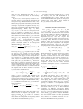
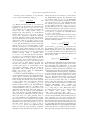
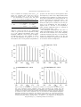
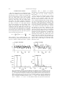
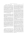
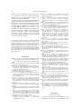
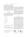
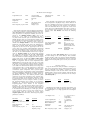
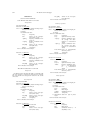
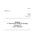
PII:
Computers & Geosciences Vol. 23, No. 9, pp. 929±945, 1997
# 1998 Elsevier Science Ltd. All rights reserved
Printed in Great Britain
0098-3004/97 $17.00 + 0.00
S0098-3004(97)00087-3
SPECTRUM: SPECTRAL ANALYSIS OF UNEVENLY
SPACED PALEOCLIMATIC TIME SERIES
MICHAEL SCHULZ1 and KARL STATTEGGER2
UniversitaÈt Kiel, Sonderforschungsbereich 313, Heinrich-Hecht-Platz 10, D-24118 Kiel, Germany, and
2
UniversitaÈt Kiel, Geologisch-PalaÈontologisches Institut, Olshausenstr. 40, D-24118 Kiel, Germany
(e-mail: [email protected])
1
(Received 19 February 1997; revised 21 May 1997)
AbstractÐA menu-driven PC program (SPECTRUM) is presented that allows the analysis of unevenly
spaced time series in the frequency domain. Hence, paleoclimatic data sets, which are usually irregularly
spaced in time, can be processed directly. The program is based on the Lomb±Scargle Fourier transform for unevenly spaced data in combination with the Welch-Overlapped-Segment-Averaging procedure. SPECTRUM can perform: (1) harmonic analysis (detection of periodic signal components), (2)
spectral analysis of single time series, and (3) cross-spectral analysis (cross-amplitude-, coherency-, and
phase-spectrum). Cross-spectral analysis does not require a common time axis of the two processed
time series. (4) Analytical results are supplemented by statistical parameters that allow the evaluation of
the results. During the analysis, the user is guided by a variety of messages. (5) Results are displayed
graphically and can be saved as plain ASCII ®les. (6) Additional tools for visualizing time series data
and sampling intervals, integrating spectra and measuring phase angles facilitate the analysis. Compared to the widely used Blackman±Tukey approach for spectral analysis of paleoclimatic data, the advantage of SPECTRUM is the avoidance of any interpolation of the time series. Generated time series
are used to demonstrate that interpolation leads to an underestimation of high-frequency components,
independent of the interpolation technique. # 1998 Elsevier Science Ltd. All rights reserved
Key Words: Spectral analysis, Harmonic analysis, Cross-spectral analysis, Irregular sampling intervals,
Interpolation, Lomb±Scargle Fourier transform.
INTRODUCTION
Spectral analysis is an important tool for deciphering information from paleoclimatic time series in
the frequency domain. It is used to detect the presence of harmonic signal components in a time
series or to obtain phase relations between harmonic signal components being present in two di€erent
time series (cross-spectral analysis).
A widely used method for spectral analysis is the
Blackman±Tukey method (BT; e.g. Jenkins and
Watts, 1968). See Figure 1. It is based on the standard Fourier transform of a truncated and tapered
(to suppress spectral leakage) autocovariance function. The major drawback of this approach is the
requirement of evenly spaced time series
…tn‡1 ÿ tn ˆ const 8n†. In general, paleoclimatic time
series are unevenly spaced in time, thus requiring
some kind of interpolation before BT spectral
analysis can be performed. As will be outlined
below, interpolation leads to an underestimation of
high frequency components in a spectrum (`reddening' of a spectrum) independent of the employed interpolation scheme.
Since cross-spectral analysis using the Blackman±
Tukey method requires identical sampling times for
both time series, that is t1 …n† ˆ t2 …n†8n, the compu929
tational e€ort (interpolation) is considerable if several time series with di€erent average sampling
intervals have to be analyzed. Furthermore, the interpolation of unevenly spaced time series may signi®cantly bias statistical results because the
interpolated data points are no longer independent.
A menu-driven PC program (SPECTRUM) has
been developed in order to avoid these problems.
SPECTRUM is based on the Lomb±Scargle Fourier
transform (LSFT; Lomb, 1976; Scargle, 1982, 1989)
for unevenly spaced time series in combination with
a Welch-Overlapped-Segment-Averaging procedure
(WOSA; Welch, 1967; cf. Percival and Walden, 1993,
p. 289) for consistent spectral estimates (Fig. 1).
Hence, unevenly spaced time series can be directly
analyzed by SPECTRUM without preceding interpolation. The main features of SPECTRUM include:
(1) autospectral analysis; (2) harmonic analysis
(detection of periodic signal components); (3) crossspectral analysis (cross-amplitude-, coherency-, and
phase-spectrum; cross-spectral analysis does not
require a common time axis of the two processed
time series); (4) analytical results are supplemented
by statistical parameters that allow the evaluation of
the results; (5) results are displayed graphically and
can be saved as plain ASCII ®les; and (6) additional
tools for visualizing time series data and sampling
930
M. Schulz and K. Stattegger
Figure 1. Computational steps in univariate spectral analysis. Left column shows estimation of spectrum of SPECMAP oxygen isotope stack (top; Imbrie and others, 1984) by Welch-OverlappedSegment-Averaging (WOSA) method. Estimated spectrum results from averaging (in this example)
three raw spectra. Right column shows steps performed in Blackman±Tukey (BT) method. Estimated
autospectrum is Fourier transform of truncated autocovariance function (acvf). Master parameters that
control results are number of segments in WOSA and truncation point of acvf (M) in BT. Unevenly
spaced time series can be directly processed using WOSA method, but not by BT method.
intervals, integrating spectra and measuring phase
angles facilitate the analysis.
The paper is organized as follows: the next three
sections provide the mathematical background of
the methods implemented in SPECTRUM.
Subsequently, the e€ect of di€erent interpolation
schemes on spectral estimates is discussed, and
®nally, two examples will be given. A description of
Spectral analysis of paleoclimatic time series
931
the installation and usage of SPECTRUM is provided in the Appendix. The paleoclimatic time series
used in this paper re¯ect late Pleistocene climate
variability as documented by marine sedimentary
records. The generated time series have properties
(length, sampling interval) similar to these data sets.
SPECTRUM can, of course, be applied to data
re¯ecting other time-scales, for example time series
documenting Holocene climate variability.
that Equation (1c) di€ers from the phase factor
given by Scargle (1989; Eq. II.2 therein). It is, however, identical to the factor used in his algorithm.
For univariate spectral analysis, tf is set to zero.
Since tf allows a virtual shift of a time series along
the time axis, it can be used to align two time series
in cross-spectral analysis (see later).
The least squares approach of the LSFT can be
considered as follows. Let
UNIVARIATE SPECTRAL ESTIMATION
x fk …tn † ˆ ak sin …o k tn † ‡ bk cos …o k tn †
Scargle (1982, 1989) developed a discrete Fourier
transformation (DFT) that can be applied to evenly
and unevenly spaced time series. Let x n x…tn †,
n = 1, 2,..., N denotes a discrete, second-order
stationary time series with zero mean. The DFT is
then given by:
X
Ax n cos …o k tn 0 †
Xk X…o k † ˆ F0
n
‡ iBx n sin …o k tn 0 †,
…1a†
with
o k 2pfk > 0, k ˆ 1, 2,:::, K, tn 0 tn ÿ t…o k †
…1b†
p
F0 …o k † ˆ …1= 2† exp fÿio k ‰tf ÿ t…o k †Šg
A…o k † ˆ
B…o k † ˆ
and
X
n
X
n
cos2 o k tn 0
sin2 o k tn 0
2X
t…o k † ˆ
ÿ1=2
…1c†
,
ÿ1=2
sin …2o k tn †
…1d†
3
1
7
6 n
arctan 4X
5:
2o k
cos …2o k tn †
…1e†
n
The constant t ensures time invariance of the
DFT, that is a constant shift of the sampling times
(tn 4tn+T0), will not a€ect the result because such
a shift will produce an identical shift in
Equation (1e), that is t 4 t + T0 and therefore
cancel in the arguments of Equations (1a) and (d)
(Scargle, 1982). Furthermore, Scargle (1982) showed
that this particular choice of t makes
Equations (1a)±(1e) equivalent to the ®t of sineand cosine functions to the time series by means of
least squares. The latter was already investigated by
Lomb (1976) in conjunction with spectral analysis,
and therefore, the method is referred to as Lomb±
Scargle Fourier transform (LSFT). The response of
a Fourier transformation to a time shift should be a
phase shift of the Fourier components. The factor
expfÿio k ‰tf ÿ t…o k †Šg in Equation (1c) produces
such a phase shift depending on the time tf. Note
…2†
be a discrete model for a signal component of x(tn)
with frequency fk. The LSFT minimizes the sum of
squares J(fk) of the di€erences between the model
from Equation (2) and the data:
min!
J… fk † ˆ
N X
nˆ1
x…tn † ÿ x fk …tn †
2
, k ˆ 1, 2,:::, K: …3†
An important aspect of the LSFT involves the
choice of K, that is the number of frequencies used
in Equation (2). Although there is no principal limit
for K, it can be anticipated that a ®nite-length time
series will only result in a ®nite amount of statistically independent Fourier components and, hence,
frequencies in Equation (2). Using Monte-Carlo experiments, Horne and Baliunas (1986) showed that
in the situation of an evenly spaced time series of
length
N, the number of independent frequencies in
ÿ fNyq , fNyq is N … fNyq ˆ 1=…2Dt† denotes the
Nyquist frequency according to the sampling theorem (e.g. Bendat and Piersol, 1986, p. 337)) and is
thus identical to a standard Fourier transformation.
The same holds true for unevenly spaced time
series, where the samples are almost uniformly distributed along the time axis. The latter usually
applies to paleoclimatic time series obtained from
marine deep-sea sediments. A signi®cant clustering
of samples along the time axis may decrease the
number of statistically independent frequencies to
1/3 N (Horne and Baliunas, 1986). In practice, it is
generally useful to choose K>N, since the resulting
oversampling results in smoother spectral estimates
(Scargle, 1982). This is equivalent to zero-padding
in standard Fourier techniques.
For unevenly spaced time series, the Nyquist frequency cannot be given, because the sampling theorem applies only to evenly spaced time series. In
this situation, an average Nyquist frequency
hfNyq i 1=…2hDti†, with hDti being the average
sampling interval, can be used as alternative.
Sections of a time series where Dtn <hDti contain
frequency information above hfNyq i. Choosing frequencies in Equation (2) above hfNyq i allows the investigation of this frequency region. Since it is
almost impossible to assess the maximum frequency
up to which an unevenly spaced time series contains
signi®cant information, this option should be used
932
M. Schulz and K. Stattegger
with great care. Selecting K such that fK ˆ hfNyq i
results in a conservative choice of the frequency
range.
A plot of jXk j2 versus frequency results in a rawspectrum, which is an inconsistent estimator of the
true spectrum (e.g. Bendat and Piersol, 1986, p. 285).
Welch (1967) proposed an estimation procedure that
results in consistent spectral estimates: a time series
of length N is split into n50 segments of length Nseg
that overlap each other by 50% (Welch-OverlappedSegment-Averaging, WOSA; Fig. 1), hence,
Nseg=2N/(n50+1). In order to avoid spectral leakage, each segment is multiplied by a taper (e.g.
Hanning-window; see Harris (1978) for an overview
of the spectral windows used in SPECTRUM) in the
time domain. The window weights wn are scaled such
P 2
that
wn ˆ NSeg . Subsequently, the n50 windowed
segments
are
Fourier-transformed
using
Equations (1a)±(1e). Averaging the n50 raw-spectra
yields a consistent estimate of an autospectrum
(Bendat and Piersol, 1986, p. 392):
G^ xx … fk † ˆ
n50
X
2
jXi … fk †j2 , k ˆ 1, 2,:::, K:
n50 Df NSeg iˆ1
In order to assess the resolution of G^ xx … fk † along
the frequency axis, the 6-dB bandwidth Bw is
commonly utilized: Bw ˆ bw Df , where bw is the
normalized bandwidth that depends on the spectral
window being used (Harris, 1978). Details of
G^ xx … fk † cannot be resolved within Bw.
BIVARIATE SPECTRAL ESTIMATION
Let x n x…tx,n †, with n = 1, 2,..., Nx and
yn y…ty,n †, with n = 1, 2,..., Ny, denote two discrete, second-order stationary time series each with
zero mean. In addition to the direct applicability to
unevenly spaced time series, the LSFT after
Equations (1a)±(1e) does not require that
tx,n=ty,n8n in order to perform cross-spectral analysis (Scargle, 1989). Therefore, two time series with
arbitrary spacing of the samples can be processed
directly without prior interpolation. We adopt the
following, conservative choices for the average
sampling interval and the fundamental frequency:
ÿ
Dtxy max hDtx i, hDty i ,
…7†
…4†
The scaling of G^ xx … fk † in Equation (4) is such that
P ^
Df
Gxx … fk † ˆ s^ 2x , with Df / 1=…NSeg hDti† being
the fundamental frequency and s^ 2x as the estimated
variance of a time series. Since the components of a
raw spectrum are w2-distributed random variables
with 2 degrees of freedom (Percival and Walden,
1993, p. 221), G^ xx … fk † also follows a w2 distribution.
Each of the n50 spectra in Equation (4) increases the
degrees of freedom, thus reducing the standard error
of the spectral estimate. However, the 50% overlap
of the n50 segments introduces a correlation between
the segments and an e€ective number of segments
ne€ results that is smaller than n50:
ÿ1
2c2
neff ˆ n50 1 ‡ 2c250 ÿ 50
,
…5†
n50
where c50 R0.5 is a constant that depends on the
applied spectral window (Welch, 1967). Harris
(1978) provides values for c50 for a variety of spectral
windows that are adopted in SPECTRUM. Finally,
(1 ÿ a) con®dence intervals for G^ xx … fk † can be calculated according to:
^
nGxx … fk †
nG^ xx … fk †
R
G
…
f
†
R
n ˆ 2neff
xx
k
w2n;a=2
w2n;1ÿa=2
…6†
(Bendat and Piersol, 1986, p. 286). Note that the con®dence intervals in Equation (6) depend on frequency. Using the logarithmic transformation
^
G^ …dB†
xx … fk † 10 log10 Gxx … fk † results in con®dence
intervals that are independent of frequency (decibel
scale; Percival and Walden, 1993, p. 257).
ÿ
Dfxy max Dfx , Dfy :
…8†
Whereas Equation (7) yields a conservative estimate
of the Nyquist frequency and therefore K,
Equation (8) ensures that the time series with the
lowest resolution in the frequency domain determines the characteristics of the cross-spectral estimates. With X(fk) and Y(fk) being the Fourier
components of the two time series, calculated
according to Equations (1a)±(1e), a consistent estimator for the complex cross-spectrum is:
G^ xy … fk † ˆ
n50
X
iˆ1
2
q
… y†
n50 Dfxy N …x†
Seg N Seg
Xi … fk † Y i* … fk † , k ˆ 1, 2,:::, K,
…9†
(cf. Bendat and Piersol, 1986, p. 407) where `*'
… y†
denotes the complex conjugate and N …x†
Seg and N Seg
are, respectively, the segment lengths that result
from splitting each of the two time series into n50
overlapping segments. Plotting jG^ xy … fk †j versus frequency, one obtains a cross-amplitude spectrum
(cross-spectrum for short). It is obvious from
Equation (9) that the values of jG^ xy … fk †j depend on
the absolute values of yn and xn. This renders the
comparison of di€erent cross-spectra dicult.
Furthermore, the estimation of con®dence intervals
for jG^ xy … fk †j is more arduous than for an autospectrum, since jG^ xy … fk †j follows a complex Wishart distribution (Koopmans, 1974, p. 280). Consequently,
the cross-spectrum itself is of little practical use
and, therefore, no con®dence intervals are determined in SPECTRUM for this parameter.
Spectral analysis of paleoclimatic time series
Of much greater importance is the coherency
c2xy … fk †, which is estimated according to:
c^2xy … fk † ˆ
jG^ xy … fk †j2
,
G^ xx … fk † G^ yy … fk †
…10†
(e.g. Bendat and Piersol, 1986, p. 137) where the
autospectra in the denominator are estimated after
Equation (4) with Df set to Dfxy and NSeg set to
… y†
N …x†
Seg , respectively N Seg . The scaling of Equation (9)
ensures that the scaling factors cancel in
Equation (10). The coherency is a dimensionless
number with 0R c^2xy … fk †R 1 for all fk. A plot of
c^2xy … fk † versus frequency is called the coherency
spectrum. Assuming a linear system, the coherency
can be interpreted as the fractional portion of the
mean square values of y(tn) that is due to x(tn) at
frequency fk or vice versa (Bendat and Piersol, 1986,
p. 172). This interpretation is, however, somewhat
delicate since it is not reversible. Hence, a high
coherency at frequency fk is not sucient to postulate that a linear relation between y(tn) and x(tn)
exists at this frequency! The coherency is zero for all
frequencies if y(tn) and x(tn) are two uncorrelated
random processes. Then, a situation where
0 < c^2xy … fk † < 1 can be caused by one of the following reasons or a combination thereof (cf. Bendat
and Piersol, 1986, p. 172): (1) noise is present in
the time series, (2) the relation between y(tn) and
x(tn) is non-linear, or (3) y(tn) is not entirely due to
x(tn), but also to other signals not taken into
account. The coherency estimator Equation (10)
is biased and leads to an overestimation of the
true coherency (Benignus, 1969). We adopt the
approximate bias correction given by Carter,
Knapp and Nuttall (1973) in SPECTRUM:
bias ‰c^2xy … fk †Š1‰1 ÿ c^2xy … fk †Š2 =neff .
To assess the statistical signi®cance of c^2xy … fk †, we
use the algorithm developed by Scannell and Carter
(1978), which is based on the cumulative distribution function for the coherency derived earlier by
Carter, Knapp and Nuttall (1973). This approach
is more accurate than the frequently employed
z-transformation: k^xy … fk † artanhjc^xy … fk †j (e.g.
Jenkins and Watts, 1968, p. 379). The disadvantage
of this transformation is that k^xy … fk † follows only a
normal distribution if 0.4R c2xy R 0.95 and ne€ r20
(Enochoson and Goodman, 1965). The latter condition can rarely be achieved with paleoclimatic
time series because the 6-dB bandwidth that is
usually required, in combination with the relatively
short time series (N < 500), generally leads to
ne€<
<20. In addition to the determination of con®dence intervals, it is also important to test whether
the coherency at some frequency can be regarded as
signi®cant. Under the null hypothesis c^2xy … fk † ˆ 0,
the false alarm level for a given a risk is
z2xy 1 ÿ a1=…neff ÿ1† (Carter, 1977). Measured coherencies less than this value should be considered
insigni®cant. Since the numerical evaluation of con-
933
®dence intervals for the coherency is time-consuming, SPECTRUM performs the calculations only
for situations where c^2xy … fk † > z2xy (cf. Bloom®eld,
1976, p. 227). Close inspection of Equation (10) for
ne€=1 shows that c^2xy … fk † ˆ 18fk independent of the
true coherency. One can expect, therefore, that for
ne€ only slightly larger than 1 (say, ne€=2 or 3),
sporadic peaks may occur in a coherency-spectrum.
Their misinterpretation as real features is, however,
avoided by the fact that the one-sided limit of z2xy
(a, ne€) for ne€ 41 equals 1 for reasonable choices
of a, say a = 0.05 or 0.01.
In the context of paleoclimatic time-series analysis, the phase relation between two variables is of
particular importance. To determine the phase-spectrum the consistent estimator
^
Qxy … fk †
f^ xy … fk † ˆ arctan
…11†
C^ xy … fk †
is used, where C^ xy … fk † and Q^ xy … fk † denote the real
and imaginary parts of G^ xy … fk †, respectively (e.g.
Bendat and Piersol, 1986, p. 124). The phase angles
are normally distributed, and an approximation of
their standard deviation (in radians) is (Bendat and
Piersol, 1986, p. 300):
ÿ
1=2
1 ÿ c^2xy … fk †
^
p :
s fxy … fk † 1
…12†
jc^xy … fk †j 2neff
It should be noted that Equation (12) implies that the
phase uncertainty approaches in®nity as the coherency approaches zero (independent of ne€). One
arrives at con®dence intervals for f^ xy … fk † by multiplying the standard deviation from Equation (12)
with appropriate quantiles of the normal distribution.
The interpretation of phase-spectra is complicated
by the fact that the inverse tangent function, which
is used to estimate the phase angles, has a periodicity of p. Estimated phase angles will always fall
within the interval [ÿp, p] or [ÿ1808, 1808] independent of the true phase angle (Fig. 2; Chat®eld,
1984, p. 200). This introduces some ambiguity into
the results that must be taken into account when
analyzing paleoclimatic data. Consider, for
example, the following two true phase angles
fxy1= ÿ 2008 and fxy2=5208. Both angles lead to
an estimated phase angle of f^ xy ˆ 1608 since they
are
folded
into
[ÿ1808,
1808]
(i.e.
ÿ2008 + 3608 = 1608; 5208 ÿ 3608 = 1608).
In order to obtain unbiased phase-angle estimates,
one has to choose identical origins of time (tf in Eq. 1c)
when processing two time series. If both time
series contain periodic components with frequency fp,
the phase-spectrum will, in general, be ¯at over a segment centered at the discrete Fourier frequency next
to fp. The width of the ¯at section is determined by the
6-dB bandwidth. However, if the sampling times di€er
between the data sets, a situation may arise where a
phase-spectrum around fp will be inclined. The reason
934
M. Schulz and K. Stattegger
Figure 2. (A) True phase-spectrum, where phase angle fxy (f) is linear function of frequency f. (B) Due
to periodicity of arctan function in p, the estimated phase-spectrum f^ xy … f † has saw-tooth shape. Slope
ts is conserved in up-sloping segments of saw-teeth. Note di€erent ordinate scales.
is that t in Eq. (1e) will no longer be identical for the
two series. Let tx,n and ty,n denote the sampling times
of two time series of length Nx and Ny, respectively. It
can be shown that an o€set t0 exists that is identical to
the di€erence in mean of the sampling times of the
two data sets:
t0 ˆ
Ny
Nx
1 X
1 X
tx,n ÿ
ty,n :
Nx nˆ1
Ny nˆ1
…13†
According to Equation (1c), this results in a linear
phase component proportional to t0. Hence, a previously ¯at phase-spectrum near fp will be inclined,
with a slope of t0 (saw-tooth shape). To avoid this
e€ect, one can shift one time series by t0 along the
time axis. This alignment can be easily achieved by
setting tf=t0 in Equation (1c) for the Fourier transform of one time series. t0 can be estimated according
to Equation (13) or from the slopes of the saw-teeth in
a phase-spectrum. The latter might work better in the
presence of noise in the data. If alignment is used, one
has to be aware that estimated phase angles
f^ …align†
… fk † are no longer direct estimates of the true
xy
phase angles. Instead, they have to be transformed
(`unaligned') according to:
f^ xy … fk † ˆ f^ …align†
… fk † ‡ t0 fk 36082n 3608,
xy
…14†
where n is an integer that ensures that f^ xy … fk † falls
into [ÿ1808, 1808]. Since Equation (14) depends on
frequency, a unique ordinate scale for a phase-spectrum does not exist if alignment is used. Finally, we
would like to remark that unexpected changes of the
sign of estimated phase angles can arise between
di€erent computer programs. This may simply be
due to di€erent assumptions regarding the time axis.
Compared to the physical time axis, the geological
age axis is reversed, that is the `past' appears on the
right-hand side of the `future'. Passing geological
ages to a computer program that assumes a physical
time axis will cause the mentioned sign change.
HARMONIC ANALYSIS
The purpose of harmonic analysis is the detection
of periodic signal components (e.g. Milankovic fre-
quencies) in a time series in the presence of noise. A
general overview on this topic can be found in
Percival and Walden (1993, ch. 10). The two
methods implemented in SPECTRUM are built on
the assumption that the noise is white noise, and
^ fk † which is identical
are based on a periodogram P…
to G^ xx … fk † from Equation (2) for n50=1 and a rectangular window. Furthermore, it is implicitly
assumed that the frequency fp of any periodic signal
component in a time series coincides with a discrete
Fourier frequency, that is that fp=fk. With a sucient oversampling in the LSFT, this requirement
can usually be ful®lled in practice.
The ®rst test was developed by Fisher (1929) and
tests whether a single periodicity exists in a time
series. The test statistic is
g
^ fk †
max1RkRK P…
,
K
X
^ fi †
P…
…15†
iˆ1
where K is the number of Fourier components.
Critical values for Fisher's test, gf, can be approximated by gf 11 ÿ …a=K †1=…Kÿ1† (Percival and
Walden, 1993, p. 491). If g>gf for some a, the null
hypothsis (signal is pure white noise) is rejected,
and it can be stated on a (1 ÿ a) con®dence level
that a periodic signal is present at the frequency
^ fk † has its maximum. The major disadvanwhere P…
tage of Fisher's test is that it tests only for the presence of a single periodic component. Siegel (1980)
extended Fisher's test for cases in which up to three
periodic components are present in a time series.
Starting from a normalized periodogram
^
~ fk † P… fk † ,
P…
K
X
^ fi †
P…
…16†
iˆ1
~ fk † that exceed
the test is based on all values of P…
some level gs instead of only their maximum as in
Fisher's test. gs is related to gf by a parameter l
with 0 < l R1. The test statistic for Siegel's test is
Tl K X
kˆ1
~ fk † ÿ lgf
P…
‡
,
…17†
Spectral analysis of paleoclimatic time series
Table 1. Coecients for computing critical values tl;a for
Siegel's test. Tabulated values extend those given by
Percival and Walden (1993, p. 493) for the situation
l = 0.4. Determination of critical values after Siegel
(1979); see also Percival and Walden (1993, p. 493)
l = 0.4
a = 0.05
a = 0.01
a = 0.9842
b = ÿ 0.51697
a = 1.3128
b = ÿ 0.59518
l = 0.6
a = 1.033
b = ÿ 0.72356
a = 1.4987
b = ÿ 0.79695
where (a)+=max (a, 0). For 20 < K < 2000 critical
values, tl;a for this test can be computed according
to tl;a=aKb (Percival and Walden, 1993, p. 493).
Empirical coecients a and b are given in Table 1
for di€erent values of a and l. Similar to Fisher's
test, the null hypothesis is rejected if Tl>tl;a. In
this situation, one or more periodic components are
935
present in the time series (at the frequencies where
~ fk † values occur). Siegel (1980) carried
the largest P…
out Monte-Carlo experiments to examine the power
of his test as a function of l in the presence of 1±3
periodic components. He found that with l = 0.6
and a single periodic component, the test has
almost the same power as Fisher's test. In the presence of two periodicities, the null hypothesis is
rejected with l = 0.6 and l = 0.4, respectively.
Three periodic components lead to a rejection of
the null hypothesis with l = 0.4.
The assumption underlying both tests, that is a
white noise background, is rarely met by paleoclimatic time series. Instead, one is more frequently
confronted with data that show a red noise background (e.g. Schwarzacher, 1993, p. 59). We will
examine how Siegel's test performs in the presence
of red noise in the ®rst example later.
Figure 3. E€ect of interpolation on autospectrum estimation. (A) Autospectrum of unevenly spaced
time series. Estimated spectral amplitudes closely match theoretical level (dashed line). (B)
Autospectrum for linearly interpolated time series. Signi®cant drop of amplitudes towards higher frequencies is in accordance with theoretical considerations (dashed line; Horowitz, 1974) and is equivalent
to variance loss (Ds2) of 54% compared to (A). (C) as (B) but for Akima-subspline interpolator.
(Theoretical spectrum not available for this situation.) (D) as (B) but for cubic-spline interpolator.
Independent of interpolator estimated spectra exhibit signi®cant bias that can be avoided by using
unevenly spaced data directly. (Settings: OFAC = 4; HIFAC = 1 [see Appendix B for description of
these parameters]; Nseg=4; Hanning-window for all analyses.).
936
M. Schulz and K. Stattegger
INTERPOLATION EFFECTS
The major disadvantage of the Blackman±Tukey
method is its inability to process unevenly spaced
data directly (cf. Fig. 1). Hence, the original data
need to be interpolated in order to obtain a regular
time axis. This section shows how frequently
employed interpolation schemes can alter the spectrum of a time series. We will consider linear,
cubic-spline, and Akima sub-spline interpolation.
The latter is a piecewise polynomial of order three
for which, in contrast to a cubic-spline function,
only the ®rst derivative must exist (Akima, 1970).
Hence, this interpolator can connect points by a
straight line. Since the LSFT allows the direct use
of unevenly and evenly spaced data, we will be able
to see the e€ect of the interpolators by comparing
the spectrum of the unevenly time series with those
for the interpolated data sets. We start by generating an unevenly spaced time series
8
X
p
sin 2pif0 tn ‡ …i ÿ 1† ,
…18†
x…tn † ˆ
4
iˆ1
with f0=0.02 kaÿ1, 0 R tn R 2100 ka and hDti ˆ 3 ka.
The unevenly spaced time axis is generated by treating Dtn as random variable that follows a gamma
distribution with 3 degrees of freedom.
Interpolation was performed such that the number
of data points was kept constant, resulting in
Dtint ˆ hDti.
Figure 3 shows the autospectra of the resulting
time series. Whereas the peak amplitudes of the
spectrum of the unevenly spaced time series
(Fig. 3A) closely match the true values, one can observe a dramatic amplitude drop at higher frequencies for the interpolated time series (Fig. 3B±D).
This e€ect is most pronounced for the linear, and
least for the cubic-spline interpolator. A comparison
of the areas under the spectra (which are equivalent
to the variance of the data) shows that a variance
loss between 33 and 54%, compared to the
unevenly spaced data set, occurs. One can therefore
expect that spectral analyses based on interpolated
data will be strongly biased. In order to exclude a
systematic error due to the LSFT, we calculated the
expected spectral amplitudes for the linear and
cubic-spline interpolators (Fig. 3B,D). Since these
closely match the estimated peak amplitude, we
exclude a bias caused by our program. The slight
underestimation compared to the theoretical amplitudes is due to ®nite length of the time series
(Horowitz, 1974).
Figure 4. Performance of Siegel's test under di€erent noise conditions. (A) Two sinusoidal waves with
periodicities of 100 and 41 ka embedded in white noise. (C) Harmonic analysis of unevenly spaced signal shown in (A): null hypothesis is rejected since test statistic (Tl=0.31) exceeds critical value
(tl;a=0.03; dashed line) and periodic components are clearly identi®ed (numbers above peaks denote respective periods). (B) as (A) but for red noise. (D) Harmonic analysis of unevenly sampled signal
shown in (B): null hypothesis is rejected (Tl=0.19; tl;a=0.03; dashed line). Periodic components can
still be recognized but additional spurious peak at f = 1/74 kaÿ1 occurs. (Settings for both tests:
OFAC = 4; HIFAC = 1; a = 0.05; l = 0.6. Note di€erent ordinate scale). See text for further details.
Spectral analysis of paleoclimatic time series
EXAMPLE 1: HARMONIC ANALYSIS
In this section, we will investigate how Siegel's
test performs in the presence of di€erent types of
noise and show that it is a useful tool for data interpretation even if the underlying assumptions are
not strictly obeyed. The ®rst test signal consists of
two sinusoidal waves (frequencies: f1=1/100 kaÿ1,
f2=1/41 kaÿ1; amplitudes: A1=A2=1) embedded in
Gaussian noise (variance s2=1). An unevenly
spaced time axis (hDti ˆ 3 ka, N = 300) was generated after Equation (18). The second time series
consists of the same sinusoidal components plus red
noise. It should therefore mimic the noise background that is typical for paleoclimatic time series
(e.g. Schwarzacher, 1993, p. 59). These data were
generated by the ®rst-order autoregressive process
(e.g. Jenkins and Watts, 1968, p. 162)
x n ˆ x nÿ1 exp…ÿDtn =tAR † ‡ Et ,
…19†
with a characteristic time constant of tAR=20 ka,
Dtn being a random variable following a gamma
distribution with 3 degrees of freedom, and Et being
Gaussian noise (s2=1). The resulting data set has
equivalent noise amplitude, average time step and
length as prescribed for the ®rst data set (signal
plus white noise).
The time series and the results of Siegel's test are
shown in Figure 4. In both situations, Tl>tl;a, and
the null hypothesis is rejected. For the white noise
case (Fig. 4C), the harmonic signal components can
be easily identi®ed. In the situation of red noise
(Fig. 4D), spurious peaks occur next to the peaks
caused by the periodic components. Taking this
result at face value, one would probably conclude
that harmonic components with periodicities of 97,
74, and 41 ka are present. At the same time, the
overall shape of the noise-induced periodogram
parts, that is those between the major peaks (cf.
Figure 4C with 4D) suggests that a red noise component is present. This should alert a user that the
assumption underlying Siegel's test might be violated. Keeping in mind that the signal-to-noise ratio
in the example was set to a low value (0.5), we still
think that Siegel' test is useful, even if the data contain a red noise background. As with any statistical
method, careful interpretation of the results is, however, required.
EXAMPLE 2: BIVARIATE SPECTRAL ANALYSIS
We will use the evenly spaced (Dt = 2 ka)
SPECMAP stack (oxygen isotope data, d18O;
Imbrie and others, 1984), which is mainly a globalice-volume signal, and an unevenly spaced
…hDti ˆ 2 ka† proxy record of North-Atlantic summer sea-surface temperatures (SST; Ruddiman and
others, 1989) to demonstrate SPECTRUM's bivariate module. We truncated the d18O time series such
937
that its maximum age corresponds to that of the
SST record (T = 650 ka). The time series are
plotted in Figure 5A and 5B. Prior to cross-spectral
analysis, we conducted harmonic analyses to ensure
that phase-angles between periodic signal components are only interpreted if corresponding harmonic signals are present in both data sets.
Otherwise, one might look at a phase angle between
a periodic signal in one time series and noise, at
that frequency, in the other data set.
We set l = 0.4 for Siegel's test (Fig. 5C, D),
since we expect more than two Milankovic periodicities in the data. In both situations, the null hypothesis is rejected, and therefore, we conclude that
harmonic signals are present (this is no surprise
because the age models of the time series were constructed by tuning the data to periodic variations of
the Earth's orbit). In the case of the SST data
(Fig. 5B), peaks at the Milankovic frequencies of
1/100 and 1/23 kaÿ1 can be clearly recognized
(Fig. 5D). With the previous example in mind, the
peaks at 1/144 and 1/41 kaÿ1 are likely to be due to
a red-noise background in the time series (the drop
in amplitude towards f = 0 kaÿ1 is caused by the
®nite length of the time series). Hence, the only periodic components present in both series are those
with frequencies 1/100 and 1/23 kaÿ1. The autospectra (Fig. 5E, F) are plotted on a decibel scale,
resulting in con®dence intervals that are independent of frequency.
Since minimum values in the SPECMAP stack,
that is ice volume minima, are expected to correlate with maxima of the SST time series, the
sign of the d18O data was changed prior to
cross-spectral analysis in order to prevent an arti®cial phase o€set by 21808. The coherency-spectrum (Fig. 5G) exhibits signi®cant coherencies at
the frequencies for which the harmonic analyses
suggested the presence of periodic components.
The phase-spectrum (Fig. 5H) indicates that iceminima lead SST maxima by 11 2188 (fk=
1/99.26 kaÿ1) and 95 2168 (fk=1/23.04 kaÿ1). The
sawtooth shape of the phase-spectrum in
Figure 5H is due to a linear phase component,
which is caused by the fact that the mean of the
SST sampling times di€ers from that of the
SPECMAP stack by 87 ka (the variance of the
SST sampling intervals increases signi®cantly with
time; Fig. 6A). As a ®rst guess, the alignment
parameter was set to this value (t0=87 ka), however, this choice did not produce a `¯at' phasespectrum around fk=1/23.04 kaÿ1. We therefore
increased t0 to 90 ka, resulting in the aligned
phase-spectrum shown in Figure 6B. The linear
trend has been successfully removed, making it
easier to measure phase angles. The aligned
phase angles are 452188 (fk=1/99.26 kaÿ1) and
1292 168 (fk=1/23.04 kaÿ1), respectively, and the
unaligned angles are calculated from these using
Equation (14):
Figure 5. Cross-spectral analysis of SPECMAP oxygen isotope (d18O; A) data and North Atlantic seasurface temperatures (SST; B). Harmonic analyses (Settings: OFAC = 5; HIFAC = 1; a = 0.05;
l = 0.4) of d18O data (C; Tl=0.64; tl;a=0.07; dashed line) and SST data (D; Tl=0.25; tl;a=0.07;
dashed line). Horizontal bar marks 6-dB bandwidth. Numbers above peaks denote respective periods.
(E) Autospectrum of the d18O time series (Settings: OFAC = 5; HIFAC = 1; Nseg=4; Welch-window).
Cross in lower-left corner marks 6-dB bandwidth (horizontal); 90% con®dence interval (vertical). (F) as
(E) but for SST data. (G) Coherency between two time series. Dashed horizontal line indicates false
alarm level (a = 0.1); 90% con®dence intervals are plotted only for coherencies exceeding this level. (H)
Phase-spectrum between d18O (inverted) and SST data. Positive angles indicate that ice minima lead
SST and vice versa. Con®dence intervals are only shown if error is less than 508 (larger errors are
marked by dots). Saw-tooth shape of phase-spectrum is caused by distribution of SST sampling times
(see text). All frequency axes were truncated below hfNyq i ˆ 0:247 kaÿ1 in order to show MilankovicÂ
range more clearly.
938
Spectral analysis of paleoclimatic time series
939
Figure 6. Aligned phase-spectrum. (A) Sampling intervals Dtn of SST data as function of time. Due to
variance increase of Dtn along time axis, mean time of the SST data htSST i is 87 ka less than that of
SPECMAP stack htSPC i. This di€erence is responsible for saw-tooth shape of phase-spectrum in
Figure 5H. (B) Aligned phase-spectrum for data in Figure 5 after aligning two series (t0=90 ka; intial
guess = 87 ka did not produce sucient ¯attening of spectrum around f = 1/23 kaÿ1). Phase angles can
be measured more easily, but must be `unaligned' prior to interpretation (90% con®dence intervals;
dots mark errors >508).
CONCLUSIONS
f^ …align†
… fk † ‡ t0 fk 3608 ÿ n 3608 ˆ f^ xy … fk †
xy
4582188 ‡ 90 ka 1=99:26 ka
ˆ 1182188
ÿ1
3608 ÿ 1 3608
12982168 ‡ 90 ka 1=23:04 kaÿ1 3608 ÿ 4 3608
ˆ 9582168:
The corrected aligned phase angles are,
course, identical to the unaligned angles.
of
A
user-friendly
computer
program
(SPECTRUM) is presented that allows direct processing of unevenly spaced time series in the context
of spectral analysis. Hence, the usual prerequisite of
data interpolation is not required. SPECTRUM
should, therefore, be of interest for users analyzing
unevenly spaced geological time series. Since the interpolation of an unevenly spaced time series is
equivalent to a low-pass ®ltering, a reddening of an
estimated spectrum is the consequence. The result-
Figure 7. Menu structure of SPECTRUM (V. 2.0).
940
M. Schulz and K. Stattegger
ing bias is not only important with regard to spectral analysis but can also a€ect time-domain
methods (e.g. ®t of autoregressive models; estimation of correlation dimension).
Spectral analysis results are supplemented by statistical tests allowing an evaluation of the results. A
combination of harmonic and cross-spectral analysis should be used if phase relationships between
harmonic signal components are of primary interest. SPECTRUM should not be used as a pure
black-box tool without checking the structure of a
time series prior to its analysis. The program may
generate meaningless results if the underlying
assumptions (weak stationarity of the processed
time series; white-noise background for harmonic
analysis) are severely violated.
AcknowledgmentsÐWe would like to thank M. Mudelsee
for discussions during various stages of the program development. Comments on the manuscript made by M.
Mudelsee and C. SchaÈfer-Neth are greatly appreciated. We
thank W. Schwarzacher and an anonymous reviewer for
their comments. This work has bene®tted from the suggestions and critique by users of earlier program versions.
MS is supported by the Deutsche Forschungsgemeinschaft
within the framework of the SFB 313. This is SFB 313
publication no. 318.
REFERENCES
Akima, H. (1970) A new method of interpolation and
smooth curve ®tting based on local procedures. Journal
of the Association of Computing Machinery 17(4), 589±
602.
Bendat, J. S. and Piersol, A. G. (1986) Random data, 2nd
edn., Wiley, New York, pp. 566.
Benignus, V. A. (1969) Estimation of the coherence spectrum and its con®dence interval using the Fast Fourier
Transform. IEEE Transactions on Audio and
Electroacoustics 17(2), 145±150.
Bloom®eld, P. (1976) Fourier Analysis of Time Series: An
Introduction. Wiley, New York, 258 pp.
Carter, G. C. (1977) Receiver operating characteristics for
a linearly thresholded coherence estimation detector.
IEEE Transactions on Acoustics Speech and Signal
Processing 25(2), 90±92.
Carter, G. C., Knapp, C. H. and Nuttall, A. H. (1973)
Estimation of the magnitude-squared coherence function via overlapped fast Fourier transform processing.
IEEE Transactions on Audio and Electroacoustics 21(4),
337±344.
Chat®eld, C. (1984) The Analysis of Time Series: An
Introduction, 3rd edn. Chapman and Hall, London,
286 pp.
Dendholm, D. (1996) GNUPLOT 3.6 user manual: (anonymous FTP: cmpc1.phys.soton.ac.uk directory: /incoming).
Enochoson, L. D. and Goodman, N. R. (1965) Gaussian
approximations to the distribution of sample coherence. Technical Report AFFDL TR 65±67. Research
and Tech. Div., AFSC, Wright±Patterson Air Force
Base, Ohio (cited in: Koopmans, 1974).
Ferraz-Mello, S. (1981) Estimation of periods from
unequally spaced observations. The Astronomical
Journal 86(4), 619±624.
Fisher, R. A. (1929) Tests of signi®cance in harmonic
analysis. Proceedings of the Royal Society of London.
Series A 125, 54±59.
Harris, F. J. (1978) On the use of windows for harmonic
analysis with the discrete Fourier trans-form.
Proceedings IEEE 66(1), 51±83 (reprinted in Kesler,
1986).
Horne, J. H. and Baliunas, S. L. (1986) A prescription for
period analysis of unevenly sampled time series. The
Astrophysical Journal 302(2), 757±763.
Horowitz, L. L. (1974) The e€ects of spline interpolation
on power spectral density. IEEE Transactions on
Acoustics, Speech and Signal Processing 22(1), 22±27.
Imbrie, J., Hays, J. D., Martinson, D. G., McIntyre, A.,
Mix, A. C., Morley, J. J., Pisias, N. G., Prell, W. L.
and Shackleton, N. J. (1984) The orbital theory of
Pleistocene climate: support from a revised chronology
of the marine d18O record. In Milankovitch and
Climate, Part I, ed. A. Berger, J. Imbrie, J. Hays, G.
Kukla and B. Saltzman, pp. 269±305. D. Reidel,
Dordrecht.
Jenkins, G. M. and Watts, D. G. (1968) Spectral
Analysis and Its Application. Holden-Day, Oakland,
CA, 525 pp.
Kesler, S. B. (ed.) (1986) Modern Spectrum Analysis II.
IEEE Press, New York, 439 pp.
Koopmans, L. H. (1974) The Spectral Analysis of Time
Series. Academic Press, New York, 366 pp.
Lomb, N. R. (1976) Least-squares frequency analysis of
unequally spaced data. Astrophysics and Space Science
39, 447±462.
Percival, D. B. and Walden, A. T. (1993) Spectral Analysis
for Physical Applications. Cambridge University Press,
Cambridge, 583 pp.
Ruddiman, W. F., Raymo, M., Martinson, D. G.,
Clement, B. M. and Backman, J. (1989) Pleistocene
evolution: northern hemisphere ice sheets and North
Atlantic Ocean. Paleoceanography 4(4), 353±412.
Scannell, E. H., Jr. and Carter, G. C. (1978) Con®dence
bounds for magnitude-squared coherence estimates.
IEEE International Conference on Acoustics, Speech
and Signal Processing, Tulsa, Oklahoma, 670±673.
Scargle, J. D. (1982) Studies in astronomical time series
analysis. II. Statistical aspects of spectral analysis
of unevenly spaced data. The Astrophysical Journal
263(2), 835±853.
Scargle, J. D. (1989) Studies in astronomical times series
analysis. III. Fourier transforms, autocorrelation functions, and cross-correlation functions of unevenly
spaced data. The Astrophysical Journal 343(2) , 874±
887.
Schwarzacher, W. (1993) Cyclostratigraphy and the
Milankovitch Theory. Elsevier, Amsterdam, 225 pp.
Siegel, A. F. (1979) The noncentral chi-squared distribution with zero degrees of freedom and testing for
uniformity. Biometrika 66(2), 381±386.
Siegel, A. F. (1980) Testing for periodicity in a time series.
Journal of the American Statistical Association 75, 345±
348.
Welch, P. D. (1967) The use of fast Fourier transform for
the estimation of power spectra: A method based on
time averaging over short, modi®ed periodograms.
IEEE Transactions on Audio and Electroacoustics 15(2),
70±73.
APPENDIX A
Setting up SPECTRUM
The hardware requirements for using SPECTRUM are:
(1) MS-DOS compatible PC with r80386 CPU and
Spectral analysis of paleoclimatic time series
numeric coprocessor, (2) VGA (or above) graphics
adapter, (3) r580 kBytes of available conventional memory/about 1 Mbytes EMS memory, and (4) MS-DOS 5.0
or higher. SPECTRUM can be obtained via anonymous
FTP from infosrv.rz.uni-kiel.de (directory: /pub/sfb313/
mschulz). Binaries are in the ®le SPEC20B.ZIP whereas
the Borland Pascal 7.0 source code can be found in
SPEC20S.ZIP. (In order to unpack the ZIP-archives
one needs either UNZIP.EXE or PKUNZIP.EXE.)
Installation of the program proceeds by copying the
archives to an appropriate directory and unzipping them
using the `-d' option. Running SPC.BAT will start the
program. If SPECTRUM refuses to work, there is usually
not enough conventional memory available; hints for troubleshooting are provided in the README.1ST ®le.
APPENDIX B
Working with SPECTRUM
After starting SPECTRUM, a title screen is displayed for
5 sec. Its display can be interrupted by pressing any key.
SPECTRUM is largely menu-driven (Fig. 7). In addition,
the input of certain parameters is simpli®ed by default
values. In the following sections, the use of the program
will be explained using data ®les located in .\DEMO. The
following acronyms and conventions will be used:
941
.
.
.
.
tN xN,
with t1<t2<... <tN and NR 2500 (maximum number of
data points). The ®rst column contains the sampling times,
and the second contains the time-dependent data.
Columns are delimited by one or more SPACES or TABs.
No particular data format (e.g. exponential) is required. It
should be noted that tn is the highest geological age. Data
®les may contain up to twenty comment lines at the beginning of a ®le. These are denoted by a `#' in the ®rst column position.
Spectral analysis results are saved as plain ASCII ®les.
SPECTRUM recognizes the di€erent output ®les by their
extensions, and therefore, these should not be modi®ed.
Three types of output ®les can be distinguished (a detailed
description of the output ®les is given in Appendix C and
D): (1) ®les with a text header showing all parameters of
the analysis (data ®les), (2) script ®les for GNUPLOT V.
3.6 (Dendholm, 1996) to plot the generated data ®les on a
variety of output devices, and (3) ®les containing data in a
format that can be easily imported into spreadsheet based
plotting programs like GRAPHER (plot ®les).
Univariate Spectral Analysis
1. ENT Enter-key
2. ESC Escape-key
3. CSL Cursor left
4. CSR Cursor right
5. CSUP Cursor up
6. CSDN Cursor down
7. HOME Home
8. END End
9. F1 F1-key
. CSUP and CSDN keys move within a menu; ENT
selects an item. ESC brings you one menu level higher.
. ESC interrupts graphic displays.
. Square brackets show either default parameters that
may be accepted by pressing ENT or options ([1], [2],...)
that are selected by pressing the appropriate number.
The module is started by selecting `Univariate' from the
main menu. Choosing `Read Data File' opens a window
for ®le selection. Use the cursor keys to move the marker
to an appropriate ®le or directory and select it by pressing
ENT. To change the current drive press the drive letter
while holding the `CONTROL'-key, for example CTRL-A
to change to ¯oppy drive A. Load the ®le
.\DEMO\XTEST.DAT for the following example. After
the ®le has been loaded, you are prompted for a label for
that time series. This label will be used on graphic screens.
If you press ENT, the ®lename will be used as default
label.
Back in the `Univariate' menu, select `Parameters/Calc'. to
de®ne the parameters for the analysis. The oversampling
factor (OFAC) determines how many frequencies are
investigated in the LSFT. It should be noted that for
OFAC>1.0, the statistical tests performed by
SPECTRUM are una€ected. In practice, OFAC = 4.0 is a
good compromise between computing time (proportional
to OFAC) and smoothness of a spectrum. This value is
default and selected by pressing ENT in this example.
Subsequently, a factor (HIFAC) must be set that determines the highest frequency fmax for the LSFT:
fmax=HIFAC hfNyq i. The resulting number of frequencies
K (cf. Eq. (2)) is then K = (OFAC HIFACNseg)/2.
Select the default value by pressing ENT. Depending on
the size of your data ®le, SPECTRUM may run out of
memory if you select too high values for OFAC and
HIFAC at the same time. In this situation, you will be
prompted to choose smaller values. The remaining parameters should be self-explanatory:
File Formats
Time series data are input into SPECTRUM as column
delimited ASCII ®les using the following format:
# Up to 20 comment lines at
# the beginning of a ®le
t 1 x1
t2 x 2
Parameter
Input
Comment
Number of segments
3
Window type
Level of signi®cance
3
2
Subtract linear trend
ENT
50% overlapping
windows in WOSA
Hanning-Window
a = 0.1 for statistical
tests
yes (each segment is
detrended)
942
M. Schulz and K. Stattegger
Logarithmic scale
ENT
Mark MilankovicÂ
frequencies
Time unit
ENT
ENT
Max. frequency to plot ENT
yes (this yields
constant con®dence
intervals)
yes
Change level of
signi®cance
unit of time in the
input ®le [ka]
display to fmax
After returning to the graphic screen (`Display Results'),
the autospectrum is displayed using a linear ordinate. In
this case, con®dence intervals are a function of frequency
and are only displayed at local maxima of an autospectrum. The horizontal line in the upper left corner of the
screen shows the 6-dB bandwidth. Press ESC to return to
the `Univariate' menu. In order to save the results of the
analysis, select `Save Results' and choose the following
options:
Note that the `Time unit' does not a€ect the calculation; it
is only used to produce a properly labeled frequency axis.
After SPECTRUM has performed the analysis, some statistical parameters are displayed. Probably the most important is the `Reliable frequency range', that is, the
interval [flow, hfNyq i], where flow is determined in such a
way that at least two full cycles are observed within each
WOSA-segment. Parts of an autospectrum outside of this
interval should be interpreted with great care! Pressing any
key returns you to the `Univariate' menu, where you
should select `Display Results' to view the autospectrum
graphically. The graphic screen shows the following features: (1) the vertical dashed lines mark the MilankovicÂ
frequencies; (2) the cross in the upper-right corner of the
screen shows the resulting 6-dB bandwidth (horizontal
line) and the con®dence interval (vertical line); and (3) the
status line at the bottom of the screen shows the label of
the data set, the 6-dB bandwidth and the level of signi®cance. A frequency marker can be activated by pressing
the `f'-key. Move the marker with the CSL, CSR, HOME
and END keys (F1 displays a help screen). The period
where the marker is located is displayed in the lower right
corner of the screen. To determine relative variance contributions of harmonic signal components in an autospectrum, an integration tool has been implemented into
SPECTRUM. To activate this tool, press the `i'-key while
the graphic screen is displayed. The area below a spectrum
in [0, fmax] is a measure of the variance of the data and is
set to 100%. The horizontal line denotes the average value
of the spectrum and is a rough estimate for a white-noise
component in a time series. Considering only those parts
of harmonic signal components, that is spectral peaks,
above this level gives an estimation of their corresponding
variance contribution. Although the assumption of harmonic signals embedded in white noise is rather strong for
paleoclimatic time series, the outlined procedure yields
results that are accurate enough for many practical situations. The selection of the integration interval is guided
by vertical lines that can be moved in the same way as the
frequency-marker. For the example at hand: (1) choose
left integration-margin: move marker to the frequency
0.0069 kaÿ1 (T = 145 ka) and press ENT; (2) choose right
integration-margin: move marker to the frequency
0.0138 kaÿ1 (T = 72.7 ka) and press ENT; (3) the result is
displayed in the lower right corner of the screen: 20.8% of
the data variance in [0, fmax] is associated with frequencies
in the selected interval. Pressing `n' or ESC gets you back
to the `Univariate' menu (you may also activate the frequency-marker again by pressing the `f'-key). Select
`Graphic Options' from the menu, and change the graphic
parameters as follows:
Parameter
Input
Comment
Logarithmic scale
Display only lower error
bars
Mark MilankovicÂ
frequencies
Max. frequency to plot
n
ENT
no
yes
ENT
yes
2
display MilankovicÂ
frequency range
ENT
no
Parameter
Input
Comment
File type
1
Use previous labels
Enter additional
information
ENT
ENT
Filename
XTEST
data ®le (with text
header) and
GNUPLOT script
yes
no (you may enter
additional text that
will be written to the
output ®le)
do not enter a ®le
extension!
Finally, the option `Show Settings' allows you to review
the main settings of the current analysis. This concludes
the ®rst example; results were saved to the ®le XTEST.PX,
which can be plotted via GNUPLOT using the script ®le
XTEST.PLT. Pressing ESC again, returns you to the main
menu.
Harmonic Analysis
Usage of the harmonic analysis module is analogous to
that of the autospectral analysis module described in the
previous subsection. The module is started by selecting
`Harmonic Analysis' from the main menu. Load the ®le
XTEST.DAT as in the previous example. After the ®le has
been loaded, you must set the parameters for the analysis
(`Parameters/Calc.'):
Parameter
Input
Comment
OFAC
HIFAC
ENT
ENT
OFAC = 4.0
HIFAC = 1.0
(NB Selection of number of segments and window type
are inapplicable here, because harmonic analysis is based
on a periodogram, i.e. a single segment and a rectangular
window.)
l for Siegel's Test
1
Level of signi®cance
1
Subtract linear trend
Mark MilankovicÂ
frequencies
Time unit
ENT
ENT
Max. frequency to plot
ENT
ENT
(l = 0.6, Test for 1±
2 harmonic
components)
a = 0.05 for
statistical tests
yes
yes
unit of time in the
input ®le [ka]
display to fmax
Spectral analysis of paleoclimatic time series
The graphic screen (`Display Results') is very similar to
that of the univariate spectral analysis. The vertical lines
mark the Milankovic frequencies, and the horizontal bar
in the upper left corner of the screen denotes the 6-dB
bandwidth. The upper and lower horizontal lines show the
critical levels for Fisher's gf) and Siegel's test (gs), respectively. Test statistic (T / Tl) and critical value (tc / tl;a) for
Siegel's test are displayed in the status line at the bottom
of the screen. Note that the statistical tests are based on
the number of independent frequencies and are therefore
independent of OFAC. In the example, the null hypothesis
(white noise) is rejected since Tl>tl;a. Periodogram values
exceeding gs (at f = 1/100 kaÿ1 and f = 1/41 kaÿ1) indicate
the presence of periodic signal components with these frequencies in the time series. Pressing F1 brings up a help
screen that provides a brief summary of the test evaluation. In addition to the frequency-marker (`f'-key), an
option to subtract harmonic signal components has been
implemented, based on a ®lter algorithm developed by
Ferraz-Mello (1981). This option may be useful if an
extreme peak in a periodogram masks minor (but signi®cant) peaks at other frequencies. For example, late
Pleistocene paleoclimatic time series frequently show a
dominant peak at f = 1/100 kaÿ1 that often covers statistically signi®cant harmonic signal components at higher frequencies. In such a case, you can subtract the 100 ka
signal component from the time series. You may also use
this option to subtract strong signal components if you
suspect them of leaking into higher frequencies. For the
present example, the option will be demonstrated for the
peak at f = 1/100 kaÿ1: (1) Pressing the `r'-key brings up a
marker line that can be moved in the same manner as the
frequency-marker; (2) move the marker to the peak at
f = 1/100 kaÿ1, and press ENT to start the subtraction of
this signal component. After the signal component has
been subtracted, the harmonic analysis is repeated (keeping the selected parameters unchanged), and the result is
automatically displayed. It may be necessary to repeat the
subtraction if a peak is not removed in a single step. This
e€ect can be due to the presence of di€erent harmonic
components with closely spaced frequencies or a quasi-periodic signal. After returning to the `Harmonic' menu, you
can modify the graphic parameters (`Graphic Options') or
review the current settings (`Show Settings'). Saving the
results is again analogous to the autospectral analysis. If
you have used the subtraction tool, you can also save the
®ltered time series.
Bivariate Spectral Analysis
To perform a cross-spectral analysis, you have to select
the option `Bivariate Analysis' from the main menu. The
usage of this module is largely identical to the univariate
module described above. The major di€erence is that two
data ®les have to be loaded. You may change the sign of
the data, which is equivalent to a phase shift of 1808. In
this situation a ` ÿ ' will be prepended to the time series
label. The subsequent parameter input allows you to
specify a virtual shift in time between the two series (alignment, t0 in Eq. (14)). Subsequent to the computations of
the spectra, you are prompted to specify the mode for the
determination of the squared coherency con®dence intervals. If you press ENT, con®dence intervals are only computed for signi®cant coherency values, that is values that
exceed the critical level.
Selecting `Display Results' after returning to the
`Bivariate' menu brings up the `Graphics' menu. From
here, you can select the appropriate graphics. You can
also modify the graphic setting from this submenu. The
display of the autospectra is identical to that described
above. Cross-spectra are presented similarly, with the
di€erence that con®dence intervals are not computed. The
horizontal line in the coherency-spectrum marks the false
alarm level. The statistical evaluation of the coherency is
943
independent of the oversampling factor OFAC. To obtain
a better readability of the phase spectrum, con®dence
intervals are only shown for absolute errors less than 508
(phase angles with errors of this magnitude exclude a
meaningful paleoclimatic interpretation). Larger con®dence intervals are marked by small circles. Pressing the
`p'-key activates a tool for measuring phase angles. The
horizontal line that appears at the center of the screen
can be moved with the CSUP, CSDN and HOME keys
(press F1 for help). The phase angle at which the marker
is located is displayed in the lower right corner of the
screen. An additional tool for the determination of the
alignment parameter is activated by the `a'-key (F1 for
help). Analogous to the integration of an autospectrum,
the vertical marker line is moved to the beginning of a
linear section of the phase-spectrum, and ENT is pressed.
After selecting the right margin of the linear section, the
corresponding alignment parameter is displayed in the
lower left corner of the screen (tau). This parameter can
be entered as `Alignment-Parameter' after selecting
`Parameters/Calc.' from the `Bivariate' menu. If alignment is used, you should never interpret phase angles
directly (see above; Eq. (14))! An `unalignment' tool that
performs the correction after Equation (14) can be activated by pressing the `u'-key while a phase-spectrum is
displayed. The marker cross can be moved as described
for the frequency/phase angle markers. The corrected
angles appear in the lower right corner of the screen.
The frequency-marker (`f'-key) and a help screen (F1) are
also available within all bivariate graphics. Saving the
results is achieved in the same way as outlined in the
univariate subsection.
Utilities
Selecting `Data File Utilities' from the main menu o€ers
the following tools:
Display Spectral Results: Option for displaying previously saved data ®les with spectral analysis results.
SPECTRUM recognizes the ®les by their extension
(PX, PY, PXY, CXY, PHI, and HFS) and by the ®rst
line of the ®le. In order to avoid errors, you should
keep the extensions and ®le headers unchanged. Plot
®les cannot be loaded with this option.
Display Time Series File: Tool to display a time series
data ®le. The sign of the data can be inverted (e.g. for
d18O data).
Average Sampling Interval: After loading a time series
data ®le, the sampling intervals Dtn are displayed as
function of time. The average sampling interval hDti
and its standard deviation are shown at the bottom of
the screen. Note that in case of evenly spaced data, a
horizontal line will appear.
Check Time Series File: SPECTRUM assumes a
monotonically increasing time vector. This tool can be
used to check data ®les prior to spectral analysis. If
duplicate sampling times are found, the corresponding
data can be replaced by their mean. A correction of a
decreasing time vector (tn + 1<tn) was intentionally not
implemented. In such cases, one should carefully look
at the data ®le.
DOS-Shell: This function allows you to leave
SPECTRUM temporarily and to access the operating
system. By typing EXIT at the command line and pressing ENT one returns to SPECTRUM.
944
M. Schulz and K. Stattegger
APPENDIX C
OUTPUT FILE FORMATS
UNIVARIATE SPECTRAL ANALYSIS
Autospectrum
File Extension: PX
Structure of a Data File:
Line 1±14: Self-explanatory header showing all parameters of the analysis
15: Empty
16: Column titles with:
Freq.:
Frequency
Gxx:
Values of the autospectrum (linear scale)
ÿd[Gxx]:
Negative con®dence inter^ xx
val of G
+d[Gxx]:
Positive con®dence inter^ xx
val of G
Gxx [dB]:
Values of the autospectrum (dB scale)
Period:
1/frequency
from 17: Results of the analysis
Structure of a Plot File:
Line 1: Column titles with:
Freq.:
Frequency
Gxx:
Values of the autospectrum (linear space)
ÿDelta:
Negative con®dence inter^ xx
val of G
Gxx [dB]:
Values of the autospectrum (dB scale)
from 2: Results of the analysis
BIVARIATE SPECTRAL ANALYSIS
Autospectra
In addition to the univariate ®le (PX), a second ®le with
the same structure is created. The latter has the extension
PY and contains the autospectral results for the second
time series.
Cross-Spectrum
File Extension: PXY
Structure of a Data-File:
Line 1±14: Self-explanatory header showing all parameters of the analysis
15: Empty
16: Column titles with:
Freq.:
Frequency
Gxy:
Values of the cross-spectrum (linear scale)
Gxy [dB]:
Values of the cross-spectrum (dB scale)
Period:
1/frequency
from 17: Results of the analysis
Structure of a Plot-File:
Line 1: Column titles with:
Freq.:
Frequency
Gxy:
Values of the cross-spectrum (linear scale)
Gxy [dB]:
Values of the cross-spectrum (dB scale)
from 2: Results of the analysis
Coherency-spectrum
File Extension: CXY
Structure of a Data-File:
Line 1±14: Self-explanatory header showing all parameters of the analysis
15: Empty
Line 16: Column titles with:
Freq.:
Frequency
Squared coherency values
Cxy2:
negative con®dence interÿd[Cxy2]:
val (ÿ9.999 4 not determined if c^ 2xy <False-Alarm
Value)
positive con®dence inter+d[Cxy2]:
val (ÿ9.999 4 not determined if c^ 2xy <False-Alarm
Value)
False-Alarm: Level of non-signi®cant
coherency values
Period:
1/frequency
from 17: Results of the analysis
Structure of a Plot-File:
Line 1: Column titles with:
Freq.:
Frequency
Cxy**2:
Squared coherency values
ÿDelta:
negative con®dence interval (`` '' 4 not determined
if
c^ 2xy < False-Alarm
Value)
False-Alarm: Level of non-signi®cant
coherency values
from 2: Results of the analysis
Phase-spectrum
File Extension: PHI
Structure of a Data-File:
Line 1±14: Self-explanatory header showing all parameters of the analysis
15: Empty
16: Column titles with:
Freq.:
Frequency
Phi:
Phase angle
2d[Phi]:
con®dence interval
Period:
1/frequency
17: Information about the sign of phase
angles
from 18: Results of the analysis
Structure of a Plot-File:
Line 1: Column titles with:
Freq.:
Frequency
Phi:
Phase angle
Delta:
con®dence interval (`` '' if
abs (Delta)>508)
Spectral analysis of paleoclimatic time series
> Maxphi:
Marks
Phi
abs(Delta) > 508
from 2: Results of the analysis
where
Harmonic Analysis
File Extension: HFS
Structure of a Data-File:
Line 1±11: Self-explanatory header showing all parameters of the analysis
12: Empty
13: Column titles with:
Freq.:
Frequency
Pxx:
Normalized periodogram
gf:
critical level for Fisher's
test
gs:
critical level for Siegel's
test
Period:
1/frequency
from 14: Results of the analysis
Structure of a Plot-File:
Line 1: Column titles being identical to the data®le
from 2: Results of the analysis
945
to produce a script ®le, SPECTRUM reads the appropriate template line by line and replaces the placeholders
listed below by their proper values. The resulting ®le has
the same name as the data ®le but with the extension
PLT.
Placeholder
%datdir%
%®lenam%
%xinfo%
%yinfo%
%xyinfo%
%timeunit%
%hifreq%
%bw%
%gxxmax%
%gxxdbmax%
%gyymax%
%gyydbmax%
%gxymax%
%gxydbmax%
%confdblo%
%confdbhi%
Meaning
path to the data ®les
®lename (without extension) of the
data ®les
label of the 1st data set
label of the 2nd data set (bivariate
only)
combination of the two previous labels
selected unit of time
max. frequency in the data ®le
(GNUPLOT's x-range is set to this
value by default)
6-dB bandwidth
max. value of the 1st
autospectrum + error (linear scale)
max. value of the 1st autospectrum
(dB scale)
as before for 2nd autospectrum
as before for cross-spectrum
lower con®dence interval for dB-scale
upper con®dence interval for dB-scale
APPENDIX D
GNUPLOT Script File Format
SPECTRUM produces script®les for GNUPLOT 3.6
(Dendholm, 1996) by replacing placeholders in templates
by their appropriate values. Three templates exist
(UNIVAR.PLT, BIVAR.PLT and HARMONIC.PLT),
one for each main module of SPECTRUM. The ®les must
be located in the same directory as SPECTRUM. In order
The templates can be changed according to a user's
requirement (e.g. by choosing a di€erent printer as
default; see the GNUPLOT manual for further details).
The above placeholders can appear anywhere in a template (multiple occurrences are allowed). The only restriction is that only one placeholder per line is possible. The
script ®les will not work with GNUPLOT 3.5, since it
does not o€er column-based computations.