1
Transactions in GIS, 2004, 8(1): 113 – 136 Technical Note A GIS-Coupled Hydrological Model System for the Watershed Assessment of Agricultural Nonpoint and Point Sources of Pollution Mauro Di Luzio Raghavan Srinivasan Texas Agricultural Experiment Station Blackland Research Center Texas A&M University Spatial Sciences Laboratory Texas A&M University Jeffrey G Arnold Grassland Soil and Water Research Laboratory United States Department of AgricultureAgricultural Research Service (USDA-ARS) Abstract This paper introduces AVSWAT, a GIS based hydrological system linking the Soil and Water Assessment Tool (SWAT) water quality model and ArcView Geographic Information System software. The main purpose of AVSWAT is the combined assessment of nonpoint and point pollution loading at the watershed scale. The GIS component of the system, in addition to the traditional functions of data acquisition, storage, organization and display, implements advanced analytical methods with enhanced flexibility to improve the hydrological characterization of a study watershed. Intuitive user friendly graphic interfaces, also part of the GIS component, have been developed to provide an efficient interaction with the model and the associated parameter databases, and ultimately to simplify water quality assessments, while maintaining and increasing their reliability. This is also supported by SWAT, the core of the system, a complex, conceptual, hydrologic, continuous model with spatially explicit parameterization, building upon the United State Department of Agriculture (USDA) modeling experience. A step-by-step example application for a watershed in Central Texas is also included to verify the capability and illustrate some of the characteristics of the system which has been adopted by many users around the world. Address for correspondence: Mauro Di Luzio, Texas Agricultural Experiment Station, Blackland Research Center, Texas A&M University System, 720 East Blackland Road, Temple, TX 76502, USA. E-mail: [email protected] © Blackwell Publishing Ltd. 2004. 9600 Garsington Road, Oxford OX4 2DQ, UK and 350 Main Street, Malden, MA 02148, USA. 114 M Di Luzio, R Srinivasan and J G Arnold 1 Introduction Increasing public concern about water quality is a major trend. It is well known that Point (PS) as well as Nonpoint (NPS), or diffuse, sources of pollution are recognized to be the leading causes of water body impairment. PS loading originates from confined areas, such as discharge pipes in factories or sewage plants. NPS loading is carried by storm water runoff and percolating water draining residential, commercial, rural, and agricultural areas where many everyday activities add polluting substances to the land. Historically, most pollution control programs have initially dealt only with PS pollution; however, all over the world and for several decades, a large percentage of water pollution has been recognized as originating from many NPSs (Novotny 1999). Typically, in less developed countries, PSs such as sewage from urban areas and NPSs such as sedimentation from deforestation or agricultural practices are the main components of pollution. In developed countries, runoff from agriculture and urban sources are the leading causes of nonpoint pollution. There is also evidence of excessive water pollution in the U.S.: coastal environments and inland streams are showing typical characteristics of eutrophication, such as high levels of nutrient concentrations causing abnormal growth of algae and other organisms in the water and the consequent unbalanced depletion of oxygen (USEPA 1999a, 2000). The control and management of water quality, particularly for impaired streams where NPSs are the overwhelming sources, would require outrageously expensive monitoring activities. The modeling alternative requires the description and understanding of several hydrologic phenomena with intrinsic spatial and temporal variation. Mathematical, hydrology-based, distributed parameter simulation models and GIS technology provide a potential synergy that appears to be the key feature for an effective understanding and interpretation of these complicated hydrologic processes connected with water quality assessment. There are diverse elements promoting the development of such systems for water resources applications (Wilson et al. 2000). Among these, the fundamental elements for our research are: (1) GISs are developed to the level that the bi-directional process of data-transfer toward and away from the model can be fully automated and enriched with interactive analysis tools for understanding the physical system and judging how management actions might affect that system’s management; and (2) the growing availability and quality of disparate supporting datasets provide convenient descriptions of important hydrologic variables that are related to chemicals, soils, climate, topography, land cover, and land use. These elements will ultimately increase the reliability of decision support tools on a watershed scale, the hydrological unit where NPSs and PSs are required to be correctly factored into an effective management system, as all human and natural activities upstream have the potential to affect water quality and quantity downstream. This paper describes the development of such a GIS-hydrological model system, ArcView-SWAT (AVSWAT), which utilizes the ArcView GIS and SWAT model and was designed to support the combined watershed assessment and analysis of NPS and PS pollution loading. Following a brief introduction to the SWAT model, AVSWAT and its illustrative application to the Upper North Bosque river watershed, which used some of the most common GIS data delivered by U.S. governmental agencies, will be discussed. © Blackwell Publishing Ltd. 2004 A GIS-Coupled Hydrological Model System 115 2 The SWAT Model The SWAT model (Arnold et al. 1998), a complex, conceptual, hydrologic, semi-distributed model with spatially explicit parameterization, builds upon over 30 years of USDA modeling experience. SWAT is a continuous time model that operates on a daily time step. The objective in model development was to predict the impact of land management on water, sediment, and agricultural chemical yields in ungauged basins. To satisfy this objective, the model is (1) physically based (as calibration is not possible on ungauged basins); (2) based on readily available inputs; (3) computationally efficient to operate on large watersheds in a reasonable time; and (4) capable of continuous simulation over long time periods, which is necessary for computing the effects of management changes. Major model components include weather, hydrology, soil temperature, plant growth, nutrients, pesticides, and land management. A complete description of the various components can be found in Arnold et al. (1998). The watershed schema is divided into sub-watersheds with unique soil/land-use characteristics or Hydrologic Response Units (HRUs). The water balance of each HRU in the watershed is represented by four storage volumes: snow, soil profile (0–2 m), shallow aquifer (typically 2–20 m), and deep aquifer (>20 m). The soil profile can be subdivided into multiple layers. Soil water processes include infiltration, evaporation, plant uptake, lateral flow, and percolation to lower layers. Percolation from the bottom of the soil profile recharges the shallow aquifer. A recession constant (Arnold et al. 1995), derived from daily stream flow records, is used to lag flow from the aquifer to the stream. Other shallow aquifer components include evaporation, pumping withdrawals, and seepage to the deep aquifer. Flow, sediment, and NPS loading from each HRU in a sub-watershed are summed, and the resulting loads are routed through channels, ponds, and reservoirs to the watershed outlet. The hydrologic components of the model have been validated for numerous watersheds, and a comprehensive validation of stream flow was performed for the entire conterminous United States (Arnold et al. 1999). The SWAT2000 version of the model (Neitsch et al. 2002) incorporates a complete revision of the nutrient cycle and pesticide components and the addition of new features like sub-daily time steps, bacteria and metal tracings. 3 AVSWAT System Development The SWAT model has been integrated with the GRASS (Geographical Resource Analysis Support System) (Srinivasan and Arnold 1994) and ArcInfo GISs (Zhou and Fulcher 1998). Both the systems were developed with an earlier version of the SWAT model and are exclusively targeted to the UNIX platform. The current version of AVSWAT (version 1.0), here described, is PC- based, designed to work with the 2000 version of the model and with ArcView version 3.x (ESRI 1996a). AVSWAT is the ultimate stage of development of a prototype designed to work only with large-scale predefined datasets of the United States (Di Luzio et al. 1997), and it has been refined to take advantage of the improved capabilities of the ArcView GIS and the contemporaneous evolution of the SWAT model. 4 Linkage Method Methods of integration of distributed water quality models with GIS have been classified using three broad, frequently overlapping and non exclusive, categories (Liao and Tim © Blackwell Publishing Ltd. 2004 116 M Di Luzio, R Srinivasan and J G Arnold Figure 1 Schematic framework of the AVSWAT system 1997): (1) loose, (2) close and (3) tight coupling. AVSWAT provides a loose coupling since ArcView is used to generate model input files (pre-processor) and display model output data (post-processor), and the interchange data files are both stored using a database (ArcView default dBASE tables) and ASCII formats. AVSWAT also provides a close coupling since modification of the GIS (customization) is made to provide an enhanced environment for data transfer between the model and the GIS database. Information between ArcView and SWAT are still passed via external files, however, the use of dBASE tables offers rapid access to the model input parameters in the GIS database. Thirdly, AVSWAT provides a tight coupling upon a further definition (Burrough 1995), since the export of data from GIS to the SWAT model and the return of results for display are accomplished by routines that are addressed directly by the interactive tools of ArcView. The routines were written in AVENUE (ESRI 1996b), which is the objectoriented scripting language for ArcView. Figure 1 shows the schematic framework of the AVSWAT system. 5 AVSWAT Software AVSWAT is implemented and distributed as an ArcView 3.x extension. The extension method is a very effective way to “plug-in” add-on software, delivering customizations and/or other software objects in order to add new functionality to ArcView. Since extensions are independent from a native ArcView project, the objects in the extension are not replicated and are never saved to the current project file; this feature is particularly advantageous for managing tools like AVSWAT that will probably be updated © Blackwell Publishing Ltd. 2004 A GIS-Coupled Hydrological Model System 117 over time. The Environmental Software Research Institute (ESRI) delivers many of its products in extensions, and developers are allowed to create their own extensions using AVENUE (ESRI 1996b). Spatial Analyst (ESRI 1996c) and Dialog Designer (ESRI 1997) are two of ESRI’s ArcView extensions used within AVSWAT to provide raster-based functionality within a traditional vector-based GIS and a way to build user interface dialogs, respectively. The AVSWAT extension introduces more than 800 AVENUE scripts, several customized menus and 55 dialogs. The supporting, context-sensitive online help software is developed in standard HTML Help format. Upon user selection, AVSWAT objects are loaded in the current ArcView session, presenting a project manager tool and leading the user through all the steps necessary to set up and refine the SWAT model simulation. 6 The Structure of the AVSWAT System As shown in Figure 1, ArcView provides both the GIS computation engine and a common Windows-based user interface within this system. AVSWAT is organized in a sequence of several linked tools grouped in the following eight modules: (1) Watershed Delineation; (2) HRU Definition; (3) Weather Station Definition; (4) SWAT Databases; (5) Input Parameterization, Editing and Scenario Management; (6) Model Execution; (7) Reading, Mapping and Charting Results; and (8) Calibration tool. Once AVSWAT is loaded, the modules get embedded into ArcView and the tools are accessed through pull-down menus and other controls, which are introduced in various ArcView graphical user interfaces (GUIs) and custom dialogs. The basic map inputs required for AVSWAT include digital elevation, soil maps, land use/cover, hydrography (stream lines) and climate. These raw data are the fundamental inputs of the first three modules that comprise the GIS data preprocessor. 7 GIS Data Preprocessor Modules 7.1 Watershed Delineation The principle underlying the development of this module, which serves as the core GIS component in AVSWAT, is that within natural landscapes, the distribution and flux of water and energy is driven by the topography. The semi-automated extraction of hydrology related topographic parameters from a Digital Elevation Model (DEM) is recognized as a functional alternative to traditional and expensive surveys and manual evaluation of topographic maps, particularly as the quality and coverage of DEM data increases. High resolution DEMs are becoming available through a number of public and commercial providers. Typical DEMs, easily available for the U.S. via the Internet, are those distributed by the U.S. Geological Survey (USGS), such as the 3 arc-second (approximately 90 m) 1:250,000-scale DEMs (USGS 1987), one arc-second (approximately 30 m) 1:24,000-scale DEMs (USGS 1990a), and 10 m National Elevation Dataset (NED) DEMs (USGS 2001, Gesch et al. 2002). In addition, the USGS is now distributing elevation data from the Shuttle Remote Topography Mission (SRTM) (USGS 2003). The 1-arc second (30 m) SRTM data are available for the continental U.S., while SRTM data is being processed at research-quality digital-elevation models one continent at a time. The data, at the resolution 90 m averaged from the original © Blackwell Publishing Ltd. 2004 118 M Di Luzio, R Srinivasan and J G Arnold 30 m data, will provide a suitable global coverage for applications of AVSWAT around the world. The Watershed Delineation module of the AVSWAT framework relies on a userprovided DEM in raster-grid format for deriving the hydrologic extent (watershed boundary) of the SWAT model application and also for the calculation of several geomorphological parameters of the whole watershed and the constituent segments. The initial basic steps of this module include the application of some elementary raster functions provided by ArcView along with its Spatial Analyst extension and the derived Hydrology Extension (Kopp 1998) for delineating streams from a raster digital elevation model. The standard methodology, which is based on the eight-pour point algorithm with steepest descent, is implemented (Jenson and Domingue 1988) along with the preprocessing procedure of filling the sink holes. In addition, AVSWAT provides the user with a set of customized and sequentially accessible tools to interactively define the watershed and stream segmentation and activate additional options in order to: 1. Define the fundamental geometric attributes of the DEM, such as value and unit of its vertical as well as horizontal resolution, which are often assumed to be uniform by default. 2. Define the boundaries of the area in which the hydrological analysis will take place, thereby reducing the computation time. This is often the case when the loaded DEM is larger than the actual study area. The user is allowed to import a predefined map (either raster-grid or vector-shape-polygon format) or interactively draw a mask over the displayed DEM. 3. Integrate a vector hydrography layer into the DEM in order to correct certain hydrologic features of a watershed that may become obscured or oversimplified during the digital delineation process. These inconsistencies are due to the problem of map scale and the lack of adequate DEM vertical resolution in areas of low relief. There are several ways to implement this method, commonly referred to as “stream burning”, although there is increasing evidence that further investigation is needed to define the process that combines accuracy and processing efficiency (Saunders 1999). The adopted algorithm simply assigns all stream grid cells with the elevation values from the original DEM while assigning all off-stream cells 500 m in addition to the DEM values. The National Hydrography Dataset (NHD) (USGS and USEPA 2000) is an example of a hydrography layer that can be used within this method for applications in the U.S. The NHD is a feature-based database that uniquely interconnects and identifies the stream segments, or “reaches”, that comprise the U.S.’s surface water drainage system. Additionally, it contains reach codes for networked features and isolated lakes, flow direction, names, stream level, and centerline representations for areal waterbodies. The Watershed Delineation module is customized in order to use this code information to trace, select, and retain only the networked features that are suitable for use with the method, such as those providing stream connectivity, that are frequently lost through reservoirs and wide rivers. A similar filtering algorithm is alternatively activated when USEPA Reach File Version 3.0 (RF3) (USEPA 1998a) data are used, whereas all the features are used when USEPA Reach File Version 1.0 (RF1) (USEPA 1998b) or any other digitized map is used as the hydrography layer. 4. Define the Stream network, Sub-Watershed outlets and Point Dischargers. Once the above preparatory steps are completed, the user is allowed to define the detail of the © Blackwell Publishing Ltd. 2004 A GIS-Coupled Hydrological Model System 5. 6. 7. 8. 119 derived stream network. This is achieved in a standard way, by entering a threshold value for the draining area, which corresponds to an equivalent contributing number of grid cells (flow accumulation grid) making up the stream branch. The subwatershed outlets are consequently located by default at the most downstream edge of each stream segment. In addition, the user in AVSWAT is allowed to modify the sub-watershed outlets, add new outlet points, or remove any of them utilizing a set of tools that involve clicking on the screen with the mouse, and geocoding point locations specified with importing tables (for example stream gauge or sampling locations). Moreover, important additional hydrologic features can be also defined in the same manner, such as point sources (PS) of discharges and watershed inlets. While point source of discharge could include sewers, treatment plants, and wastewater discharge, the watershed inlet is used when an upstream portion of the watershed area is not directly modeled (because other simulation models or observed data are used) and is thereby excluded from the watershed modeling framework. For both types of locations, the user will provide the SWAT model with discharge data records that will be routed through the stream network. The first location type represents the fundamental element allowing the inclusion of the PSs within the study watershed for the evaluation of their possible importance in a water quality assessment. In addition the watershed inlets allow for restricting the simulation, the collection of data as well as the water quality assessment in those cases where particular target sub-watershed and reach segments of any stream order need to be studied. This is particularly important since stream segment as well as watershed assessments are required for the support of most Total Maximum Daily Load (TMDL) programs (USEPA 1999b). Define the main watershed outlet(s) through a customized selection tool. The watershed and sub-watershed boundary definition is performed by a standard process, which includes tracing the flow direction from each grid cell until either an outlet cell or the edge of the DEM grid extent is encountered. The watershed, as well as the sub-watershed boundaries are created and the user completes this section reviewing and modifying the respective outlets in order to make the new defined set of subwatersheds as needed. Define geomorphological parameters. Sub-watershed and stream reach parameters are defined based on the elevation values, the previously defined segmentation, and the drainage direction vector of each cell, whose dimension becomes the basic unit for all the calculations. Developed raster-grid and map algebra functions calculate parameters like area, accumulated area, and slope of each sub-watershed, slope and length of the mainstream channel flowing from each sub-watershed inlet to the respective outlet, and for the longest stream channel, extending from each subwatershed outlet to the most distant point in the sub-watershed. Based on statistical relationships reported in literature, other parameters are indirectly deduced, such as the field slope length (Wischmeier and Smith 1978), stream reach depth, and width (Allen et al. 1994). Make available a report describing the topographic aspect of the watershed while the set of calculated geomorphological parameters are stored as attributes of the derived vector-shape themes. Define lake and reservoir locations. These important hydrological features can be located within the stream network, using a click and drop tool and/or importing location tables similar to those described for (4) above. © Blackwell Publishing Ltd. 2004 120 M Di Luzio, R Srinivasan and J G Arnold 7.2 HRUs Definition The application of this module completes the hydrologic scheme of the watershed and the intermediate, dynamically developed watershed database needed to provide the inputs to the SWAT model. For the U.S., typical inputs for this model are the land use dataset used for U.S. watersheds based on Anderson level II classified land use/land cover layer, created using the 1:250,000 scale USGS map series (USGS 1990b), USGS National Land Cover Database (NLCD) (Vogelmann et al. 2001), USDA-NRCS State Soil Geographic Database (STATSGO) (USDA NRCS 1992), and the continuously evolving Soil Survey Geographic (SSURGO) (USDA NRCS 1995) soil association datasets. However, the user is allowed to input any other source of land use/land cover or soils data, either in raster-grid or vector-shape format. This module is used to define the distribution and combination of the land use and soil categories within the watershed and sub-watersheds. A set of tools allows the user to load and clip land use and soil maps to the watershed boundary. The watershed clipped land use and soil maps, automatically re-sampled at the DEM resolution, must then be reclassified into the various SWAT defined crop or urban land type categories. This task can be accomplished either by using a developed tool to click and drop the categories of the target model or by applying predefined look-up tables. The derived thematic maps are overlaid using raster functions, which are more computationally efficient when compared to the equivalent vector functions. On the basis of the determined distribution of the land use/soil combinations (HRUs) for the model simulation, the user is provided with the options to either use the predominant unit within each subwatershed or controlling the total number of modeling units based on specified thresholds of land use and soil percentages. Detailed reports of the current HRU definition results are provided for the user to review. 7.3 Weather Stations Definition This module allows the user to import into the project the station locations and input the respective time series for rainfall, temperature, solar radiation, relative humidity, and wind speed. The interface not only facilitates the geocoding of the station locations and associates each sub-watershed to the closest one, but it also labels the missing daily data records that the SWAT model will be able to generate at run time using a built-in weather generator. In fact, all the weather data are optional since the model is able to generate a dataset based on statistical parameters of specified weather stations provided using the following SWAT Databases module. 8 SWAT Database Module This module contains seven basic, fully developed databases stored by AVSWAT using the dBASE format. Figure 2 shows the interface menu allowing the user to select and start an editing section. In addition, Figure 2 shows the number of parameters and the number of entry records included in each of these databases, two of which are described below: 1. The Weather Generator Database: As mentioned above, the SWAT model is able to generate climate data based on a set of statistical parameters. A database containing © Blackwell Publishing Ltd. 2004 A GIS-Coupled Hydrological Model System 121 Figure 2 SWAT Database editor menu within AVSWAT interface. The number of parameters and records of each distributed database are indicated. Only one entry example is provided statistical data for 1,041 weather stations in the U.S. (Nicks 1985) is distributed and available for modeling watersheds in the U.S. If different data are adopted, the user is allowed to add new entries into an established AVSWAT database (Userstations), applying a dedicated interface tool. 2. The Soils Database: While the AVSWAT package does not include GIS data, a referenced database containing the soil parameters derived from STATSGO (Baumer et al. 1994) for modeling watersheds in the U.S. is provided. Using these data, the soil series within the STATSGO database will be referenced within the HRU Definition module using any combination of Sequence Number, Name, Soil5ID and the map unit (Stmuid) identifiers. If a different data source is adopted, the user is allowed to add new entries, referenced using the Name of the soil, into an established AVSWAT database (Usersoils) and applying a dedicated interface tool. The remainder of the SWAT databases contain default parameters used within the mathematical equations of the model for the simulation of fundamental land use/soil management components of the model system. The interface contains tools that allow the users to edit and/or add new entries in any of these databases in order to match the model assumptions of the land management with those within the case study watershed: 3. Plant growth: This database contains information required to simulate the growth of the most common plant species, such as Nitrogen uptake and the Minimum (base) temperature for plant growth. 4. Urban land use: This database contains parameters required to simulate urban areas, such as the Wash-off parameter for removal of constituents from impervious areas and Curb length density for different urban land types. 5. Tillage: This database contains parameters required to simulate the redistribution of nutrients, pesticide and residue in the soil profile for the most common tillage implements. Examples include the Mixing depth and Mixing efficiency parameters. © Blackwell Publishing Ltd. 2004 122 M Di Luzio, R Srinivasan and J G Arnold 6. Fertilizer/manure: This database contains parameters that quantify the relative fractions of nitrogen and phosphorus pools, and the bacteria contents in the most common fertilizers. Examples include the Fraction of mineral Nitrogen, Fraction of organic Phosphorus and Concentration of persistent Bacteria. 7. Pesticide: This database contains parameters related to the fate and transport of the most common pesticides, such as the Wash-off fraction and Degradation half-life. See Neitsch et al. (2002) for a complete description and references for the parameters contained in these databases. 9 Input Parameterization, Editing, Scenario Management, Point Source and Model Execution Modules These modules complete the input data preprocessor and start a model simulation. The Input Parameterization module, based on the previously defined watershed segmentation, geocoding of point sources of discharge, HRU and weather station definitions, and the content of the databases, creates and automatically populates a watershed-related database (dBASE® tables) containing the input parameters of the model. The actual input files of the model, in ASCII format, are also concurrently built up. The inputs are used within 15 SWAT model components as shown in Figure 3 along with the respective content. More than 90 parameters are defined for the entire watershed, 400 for each sub-watershed and 300 for each HRU. This figure also reports the number of parameters used by each SWAT model component and the AVSWAT dialog menu that allows selection and initiation of an editing session. Each editing dialog tool of the Editing module allows the user to review and edit any of the included parameters, check the validity based on predefined and editable range values, and to copy a selected record to other target sub-watersheds and/or land use-soil combination input sets. The input parameters associated with the reservoirs that were located during the watershed delineation, can also be revised with a separate tool. The NPSs are assessed with the help of the Scenario Management module, a tool editor that itemizes the SWAT input for land and water management practices, such as planting, harvest, tillage operation, irrigation, nutrient and pesticide applications scheduled by date or by crop heat units within any number of crop rotations. This tool also allows specification of change of land use, agricultural and urban management scenarios in any specific HRU and building a scenario management configuration file intended to be a set of scheduled operations. This is particularly useful for saving scenario settings that, in this manner, can be exported and loaded into other editing sessions or watershed projects. Figure 4a shows the input management tool dialog in AVSWAT. The PSs are integrated with the help of the Point Source module, an input tool allowing the merging of discharge records with the current watershed simulation. These data may be provided in summary on a daily, monthly, yearly, or constant average basis. The loading variables are: water, sediment, organic N, organic P, nitrate, soluble P, ammonium, nitrite, maximum three metals, and bacteria. Figure 4b shows the point discharge input dialog in AVSWAT. A similar tool handles discharges from sources associated with different land areas, named watershed inlet loading sources. © Blackwell Publishing Ltd. 2004 A GIS-Coupled Hydrological Model System 123 Figure 3 Input data and calling menu dialog within AVSWAT interface. The number of parameters of each distributed database is indicated As mentioned above, point source, as well as inlet watershed dischargers, are located within the watershed framework during the watershed delineation. The Model Execution Module allows the user to set final simulation control codes, such as: evapotranspiration method, length of simulation (beginning and ending day of simulation), type of simulation, time step of inputs and outputs and several others. This module then allows the start of the SWAT model simulation after an optional range checking of all necessary input files. © Blackwell Publishing Ltd. 2004 124 M Di Luzio, R Srinivasan and J G Arnold Figure 4 Input dialogs in AVSWAT: (a) Land use and soil management dialog (b) Point discharge loadings dialog (the Stephenville wastewater values of the Upper North Bosque application example are reported) 9 Reading, Mapping and Charting Results Module This module is the simulated data postprocessor allowing for the conversion of the main SWAT model outputs in ASCII to dBASE tables. The main converted output tables are: 1. Sub-watershed output (or BSB) table: this table contains summary information for each of the sub-watersheds in the watershed. The 14 variables in this table (see Table 1 Table 1 Summary of the SWAT model variables in the sub-watershed output table. Water Yield (mm) Potential Evapotraspiration (mm) Actual Evapotransipration (mm) Soil Water Content (mm) Snow or ice melt (mm) Percolation (mm) Surface Runoff (mm) Groundwater contribution (mm) Sediment Yield (tons/ha) Organic Nitrogen (kg/ha) Organic Phosphorus (kg/ha) Nitrate (kg / ha) Soluble Phosphorus (kg/ha) Mineral Phosphorus (kg/ha) © Blackwell Publishing Ltd. 2004 A GIS-Coupled Hydrological Model System 125 for details) are the total amount or weighted average of all HRUs within the sub-watershed. 2. Main channel output table (or RCH) table: this table contains more detailed summary information for each of the routing reaches in the watershed. The 42 variables in this table include pesticides, metals, and pathogens. 3. HRU output (or SBS) table: this table contains 58 detailed parameter summaries for each of the HRUs in the watershed. Other converted tables contain detailed information for ponds, wetlands, and depressional/impounded areas within the HRUs (40 variables in the WTR table) and reservoirs (36 variables in the RSV table) in the simulated watershed. See Neitsch et al. (2002) for a complete description of these data tables. Another tool component of this module allows for the presentation of the SWAT model output both in graphic and map formats at either the sub-watershed or stream reach levels (BSB and RCH table). The tool operates the selection of the target subwatershed records in the table and joins them to the original segmented watershed map. 10 Calibration Module This module allows the user to interactively perform manual model calibrations. The user can target the model parameters listed in Table 2, considered the most sensitive (Neitsch et al. 2002), set their variations either within or outside user-defined ranges (in percent of the current value or by an absolute value), apply them for target subwatersheds and land use-soil combinations, and re-run the model. The calibration scenarios can be saved, later modified or exported for use within the same or another watershed project. Each calibration scenario provides independent outputs, thereby allowing an immediate comparison using the previously described module. 11 Example Application An application of AVSWAT to the Upper North Bosque River (UNBR) watershed is presented below. This example is provided with the sole intent of showing the steps followed to apply AVSWAT and verify its primary outputs, water discharge and sediment yield, in comparison with a set of observed data and previous simulations in the same location. The UNBR watershed covers approximately 932 km2 in the upper portion of the North Bosque River (NBR) watershed, almost entirely within Erath County in central Texas (Figure 5). Dairy farming is the predominant agricultural practice in the UNBR watershed since more than 70 dairies with over 30,000 milking heads of cattle are found in this area (Kiesling et al. 2001). This environment creates a particular water quality concern since the Bosque River discharges into Lake Waco, which is used for the public drinking water supply for the City of Waco and several adjoining communities. The Texas Natural Resource Conservation Commission (TNRCC) and Texas State Soil and Water Conservation Board (TSSWCB) are working with the EPA to ensure that the new TMDL program complies with federal regulations and guidance. The program includes extensive sampling and the use of computer simulation models to identify sources of © Blackwell Publishing Ltd. 2004 126 M Di Luzio, R Srinivasan and J G Arnold Table 2 Modifiable parameters using the Calibration tool within AVSWAT. Minimum value of USLE C factor for water erosion applicable to the land cover/plant. Maximum melt rate for snow during (mm/°C/day) where °C pertains to the air temperature. Minimum melt rate for snow during the year (occurs on winter solstice) (mm/°C/day) Linear parameter for calculating the maximum amount of sediment that can be reentrained during channel sediment routing Exponent parameter for calculating sediment reentrained in channel sediment routing Nitrogen percolation coefficient. Phosphorus percolation coefficient. Phosphorus soil partitioning coefficient. Initial labile (soluble) P concentration in surface soil layer (kg/ha). Initial organic N concentration in surface soil layer (kg/ha). Initial organic P concentration in surface soil layer (kg/ha). Initial NO3 concentration (mg/kg) in the soil layer . Baseflow alpha factor (days). Threshold depth of water in the shallow aquifer required for return flow to occur (mm). Groundwater “revap” coefficient. Threshold depth of water in the shallow aquifer for “revap” to occur (mm). Soil evaporation compensation factor. Average slope steepness (m/m). Average slope length (m). Temperature laps rate (°C/km). Channel cover factor. Channel erodibility factor. Effective hydraulic conductivity in main channel alluvium (mm/hr). Biological mixing efficiency. USLE equation support practice (P) factor. SCS runoff curve number for moisture condition II. Available water capacity of the soil layer (mm/mm soil). nutrients and to determine how they are partitioned throughout the watershed, development of water quality monitoring plans, and implementation programs to improve water quality. The Texas Institute for Applied Environmental Research (TIAER) at Tarleton State University started monitoring UNBR in 1991 (McFarland and Hauck 1999) using stormwater monitoring sites instrumented with automated samplers (Figure 5). Table 3 provides a summary of the various steps involved in a generic implementation of AVSWAT and the one described here. As shown in Figure 1, the basic GIS databases needed for the AVSWAT are the digital elevation model data (DEM), hydrography (optional), land use, soil and weather station locations, and associated observed data. The following layers have been used for this application: 1. Three arc-second, 1:250,000-scale, USGS DEM (grid format); 2. NHD dataset for cataloging unit 12060204 (shape-polyline format); 3. 1:250,000-scale, USGS Land Use and Land Cover (LULC) data (shape-polygon format); © Blackwell Publishing Ltd. 2004 A GIS-Coupled Hydrological Model System 127 Figure 5 The Upper North Bosque River (UNBR) watershed in central Texas 4. USDA-NRCS STATSGO soils map (shape-polygon format); 5. Daily rainfall and temperatures from 14 gauges within the watershed including water sampling and National Weather Service stations. All these input layers were aligned to a common projection (Albers Conical Equal Area). The DEM resolution was 86 m. As reported in Table 3, the sample watershed has been delineated using the location of the sampling station BO070 as the main outlet and segmented into 55 sub-watersheds, and further subdivided into 171 HRUs. Tables 4 and 5 report the distribution of the land use and soil classes within the watershed. The daily PS loads, reported by Saleh et al. (2000) for a composite modeling application in the UNBR watershed, for the Stephenville wastewater treatment plant were used (see also Figure 4b). The management of dairy wastes is a key objective for the UNBR programs in order to lessen runoff pollution. The AVSWAT interface allows for the consideration of dairy wastes alternatively as point discharges or as nonpoint sources in order to simulate the most common, and generally the most desirable, method of utilizing manure that involves spreading it over the land to retain the value of the nutrients and organic matter. The second alternative has been used: the land use map has been slightly modified to contain the land areas of manure application and to apply associated management scenarios, as accomplished by Santhi et al. (2001) for an extensive application of an earlier version of the SWAT model and GIS system to the entire NBR watershed. Using similar calibration settings, the application of AVSWAT generated the simulation results reported in Table 6 and Figure 6 for the period from January 1993 to July 1998. The © Blackwell Publishing Ltd. 2004 128 M Di Luzio, R Srinivasan and J G Arnold Table 3 Steps in implementation of the AVSWAT (in Italic the Upper North Bosque application settings) Start an AVSWAT project Step 1. Load the AVSWAT extension checking the box labeled “AVSWAT2000” within the ArcView Extensions dialog Step 2. From the AVSWAT project manager start a New project Watershed Delineation Step 3. Load the DEM (grid format) (resolution 3 arc seconds = 86 meters) and set the DEM Properties, horizontal-vertical units (meters-meters) [optional] Define the working zone using the Focusing Watershed Area tools (either manually or using a predefined a map) [optional] Define the hydrography layer (NHD, RF3, RF1 or used defined) for the Burn-in method application (NHD dataset for cataloging unit 12060204) Step 4. Apply the Preprocessing of the DEM Step 5. Enter the Threshold Area (1100 ha) and Apply the Stream Definition [optional] Refine step 4 Step 6. [optional] Review the sub-basin Outlet set (Add Hico Main Outlet, Remove and Redefine), set Point Source of Pollution location and Inlet of draining watersheds Step 7. Select the Main Watershed Outlet(s) [optional] Undo and return to Step 5 Step 8. Apply the Calculation Subbasin Parameters Step 9. Locate Reservoirs (Add) [optional] Review Reservoir locations (Remove, Add) HRUs definition Step 10. Load the Land Use map (shape or grid format) (LULC and STATSGO) Step 11. Reclassify the map on the watershed area using a click and drop tool or a lookup table (used pre-built look-up tables) Step 12. Load the Soil map (shape or grid format) Step 13. Reclassify the map on the watershed area using a click and drop tool or a lookup table Step 14. Apply the Overlay Step 15. Select and Apply land use/soil distribution option: either Dominant or HRU. For the second option specify Land Use % and Soil % thresholds (20–10) SWAT Model Input File Creation, Execution, Output File Extraction, Charting and Mapping Step 16. Import Weather Station locations. These stations provided statistical parameters for weather data generation (used pre-built look-up tables) [optional] Import Stations locations and data sets for: rainfall, temperature, relative humidity, solar radiation and wind speed (used rainfall and temperature stations) Step 17. Write the Default input data [optional] Review and Edit any of input files. Make an agricultural and/or urban management scenarios (dairy wastes application areas) Step 18. Set up and execute SWAT simulation [optional] Verify validity of input parameters ranges Step 19. Read outputs [optional] Apply the Calibration Tool (see description) Step 20. Chart and/or Map the output tables © Blackwell Publishing Ltd. 2004 A GIS-Coupled Hydrological Model System 129 Table 4 Land use – land cover classes used for AVSWAT in UNBR watershed. The corresponding SWAT model crop growth or urban classes are also indicated Land use – Land cover class SWAT Class % Watershed Area Range-Brush Pasture Range-Grasses Water Wetlands-Non-Forested Commercial Forest-Deciduous Forest-Evergreen Forest-Mixed Agricultural Land-Generic Industrial Transportation Residential-Medium Density Orchard RNGB PAST RNGE WATR WETN UCOM FRSD FRSE FRST AGRL UIDU UTRN URMD ORCD 0.38 0.10 39.44 0.34 0.02 0.42 1.41 0.07 3.02 53.34 0.01 0.09 1.30 0.06 Table 5 Soil – STATSGO class distribution using AVSWAT in UNBR watershed Stmuid % Watershed Area TX285 TX612 TX094 TX442 TX521 TX066 TX403 TX145 1.53 46.78 1.16 43.55 1.24 0.25 4.74 0.75 Table 6 Sampling station BO070 at Hico. Averaged observed and simulated water discharge and sediment yield in UNBR watershed using AVSWAT 1.0. Analysis period January 1993 – July 1998 Variable Observed Simulated Nash and Sutcliffe (1970) E (monthly time step) Water Discharge (m3/s) Sediment Yield (t) 4.43 4489.90 4.29 3625.91 0.82 0.78 © Blackwell Publishing Ltd. 2004 130 M Di Luzio, R Srinivasan and J G Arnold Figure 6 Sampling Station BO070 at Hico. Observed and simulated values in UNBR watershed using AVSWAT 1.0. Analysis period January 1993-July 1998 (a) Water flow (b) Sediment yield © Blackwell Publishing Ltd. 2004 A GIS-Coupled Hydrological Model System 131 results, in their comparison with the measured data, resemble those of Santhi et al. (2001) and follow closely those of Saleh et al. (2000), thereby representing an initial verification of the AVSWAT system. Figure 7 shows the spatial distribution of three variables (sediment yield, organic phosphorus, and soluble phosphorus) in the UNBR watershed as obtained from the mapping outputs of AVSWAT. The graphs in Figures 6a and 6b were produced using the Microsoft Excel software and the AVSWAT dBASE tables. Once again these maps, as well as the simulation outputs, are reported only to illustrate the capabilities of AVSWAT and are not intended to evaluate the water quality problems in the UNBR watershed. The UNBR case study shows that AVSWAT minimizes the time required for assembling the extensive input data needed for distributed, continuous modeling of water quality at the watershed scale. In addition, the following features make this system distinctively useful: 1. The user friendliness, enhanced by a mouse driven approach and the useful context-sensitive on-line help, allows applications by average users with limited GIS skill; 2. The usage of well known and established input formats (grid and shape format files) and flexibility of these databases allow applications virtually anywhere; 3. The watershed segmentation is particularly facilitated and enhanced with tools for the definition of fundamental hydrologic features for a complete water quality assessment; 4. The generally tedious and complicated task of the reclassification of raw raster GIS data, such as the land use and soil maps, is simplified and provides a direct linkage to the internal databases; 5. The system allows for the simple inclusion of articulated management scenarios, reflecting spatial and temporal changes in land use practices, as well as point source loading records with various levels of detail; 6. The ability to run the model interactively and for quick basic calibration of the simulations; 7. The ability of compare the various management scenarios across long simulation periods (100 years or more) using the model weather generator; 8. The editable SWAT databases, the management and calibration configuration files, enhance the transferability of data and modeling insights within the same or other watershed application projects; 9. The application provides detailed visualization of the model outputs in spatial, tabular and graphical forms, at the sub-watershed and stream reach level, thereby allowing the identification of georeferenced critical areas as well as water with pollutant concentration and loading over established standards. dBASE tables are also easily importable within external graphical and/or statistical packages for more detailed analysis; 10. The incorporation of the application completely in ArcView allows the user to embrace all the geoprocessing capabilities of this GIS and the supporting software developed with the extension method, both by the user community and by ESRI. These important features help to improve the analysis of point and nonpoint point sources and refine the quality of watershed management decision making. © Blackwell Publishing Ltd. 2004 132 M Di Luzio, R Srinivasan and J G Arnold Figure 7 Example application of AVSWAT in the Upper North Bosque River. Output mapping of (a) Sediment Yield (b) Organic Phosphorus (c) Soluble Phosphorus © Blackwell Publishing Ltd. 2004 A GIS-Coupled Hydrological Model System 133 Figure 7 (Continued ) 12 Conclusions The assessment of the combined, cumulative impacts of both PS and NPS is recognized to be a worldwide critical issue and of particular concern for the U.S. Environmental Protection Agency (EPA) regulating the development of the TMDL programs in the United States. In this paper, we presented AVSWAT version 1.0, an integrated GISmodeling environment for the combined assessments of point and nonpoint source pollution on a watershed scale. AVSWAT extends the ArcView GIS engine to provide adequate and efficient data support to SWAT, a mathematical, hydrology-based simulation model with specific spatial parameterization, reinforcing the understanding and interpretation of complicated hydrologic processes. This is accomplished by several modules that offer a full range of user-friendly and interactive input/output manipulation capabilities in order to help the user perform numerous tasks. These include: segmenting and dimensioning the watershed based on the digital description of topography, importing and formatting the supporting data, analyzing and displaying output data from the model simulation, formulating management scenarios and performing basic calibration. The illustrative example of the Upper North Bosque River watershed represents an initial hydrologic verification of the system, thereby confirming that the system is highly intuitive and a valuable resource for carrying out water quality analysis projects at the watershed level. The system can also support water quality analysis at the single stream segment scale as required for the support of most TMDL programs. In addition, the system, being PC-based and allowing the usage of input data with © Blackwell Publishing Ltd. 2004 134 M Di Luzio, R Srinivasan and J G Arnold established formats, substantially increases the number of potential users around the world. AVSWAT is being used in several research projects and as an educational tool in college environmental classes. The AVSWAT user community is distributed worldwide. A Web site is maintained (http:/www.brc.tamus.edu/swat/avswat/) to let the user download the software and the user’s manual and to maintain a record of the latest developments. A discussion forum website (http://sslgtw01.tamu.edu/swat/) allows the user community to share application experience and suggestions. Future developments of the system will include a UNIX version, the capability of plug-in (customized extension) functionality, the automatic integration of remote datasets through the Internet, and finally the conversion of the system to the ArcGIS architecture with the inclusion of the Arc Hydro (ESRI 2002) data model functionality. Acknowledgements The authors thank the Texas Institute for Applied Environmental Research (TIAER) at Tarleton State University for providing the water quality data for the Upper North Bosque Watershed. References Allen P M, Arnold J G, and Byars B W 1994 Downstream channel geometry for use in planninglevel models. Water Resources Bulletin 30: 663 –71 Arnold J G, Allen P M, Muttiah R S, and Bernhardt G 1995 Automated base flow separation and recession analysis techniques. Groundwater 33: 1010 – 8 Arnold J G, Srinivasan R, Muttiah R S, and Williams J R 1998 Large area hydrologic modeling and assessment: Part I, Model development. Journal of American Water Resources Association 34: 73 – 89 Arnold J G, Srinivasan R, Muttiah R S, Allen P M, and Walker C 1999 Continental scale simulation of the hydrologic balance. Journal of American Water Resources Association 35: 1037– 52 Baumer O, Kenyon P, and Bettis J 1994 MUUF Volume 2.14 User’s Manual. Lincoln, NE, Natural Resource Conservation Service, National Soil Survey Center Burrough P A 1995 Opportunities and limitations of GIS-based modeling of solute transport at the regional scale. In Corwin D L and Loague K (eds) Applications of GIS to the Modeling of Non-Point Source Pollutants in the Vadose Zone. Madison, WI, Soil Science Society of America: 19 –38 Di Luzio M, Srinivasan R, and Arnold J G 1997 An Integrated User Interface for SWAT Using ArcView and AVENUE. St. Joseph, MI, American Society of Agricultural Engineers Paper No 97–2235 ESRI 1996a What’s New in ArcView GIS 3.0. Redlands, CA, Environmental Systems Research Institute ESRI 1996b Using AVENUE. Redlands, CA, Environmental System Research Institute ESRI 1996c Using the ArcView Spatial Analyst. Redlands, CA, Environmental System Research Institute ESRI 1997 Using the ArcView Dialog Designer (Version 1.0). Redlands, CA, Environmental System Research Institute ESRI 2002 ArcHydro: GIS for Water Resources. Redlands, CA, Environmental System Research Institute Gesch D B, Oimoen M J, Greenlee S K, Nelson C A, Steuck M, and Tyler D J 2002 The National Elevation Dataset. Photogrammetric Engineering and Remote Sensing 63: 5 –11 © Blackwell Publishing Ltd. 2004 A GIS-Coupled Hydrological Model System 135 Jenson S and Domingue J 1988 Extracting topographic structure from digital elevation data for Geographic Information System analysis. Photogrammetric Engineering and Remote Sensing 54: 1593 –1600 Kiesling R L, McFarland A M S, and Hauck L M 2001 Stream Community Responses to Eutrophication from Nonpoint Source Nutrient Loading. In Proceedings of American Water Resources Association Spring Specialty Conference on Water Quality Monitoring and Modeling: 181– 6 Kopp S 1998 Developing a hydrology extension for ArcView Spatial Analyst. ArcUser April-June: 18 –20 Liao H and Tim U S 1997 An interactive modeling environment for nonpoint source pollution control. Journal of American Water Resources Association 33: 591– 603 McFarland A M S and Hauck L M 1999 Relating agricultural land uses to in-stream stormwater quality. Journal of Environmental Quality 28: 836 – 44 Nash J E and Sutcliffe J V 1970 River flow forecasting through conceptual models: Part 1-A, Discussion of principles. Journal of Hydrology 10: 282–90 Neitsch S L, Arnold J G, Kiniry J R, Srinivasan J R, and Williams J R 2002 Soil and Water Assessment Tool User’s Manual (Version 2000). College Station, TX, Texas Water Resources Institute Technical Report No GSWRL 02-02, BRC 02- 06 Nicks A D 1985 Generation of Climate Data. In Proceedings of the Natural Resources Modeling Symposium, 16 –20 October, Pingree Park, Colorado: 297–300 Novotny V 1999 Diffuse pollution from agriculture: A worldwide outlook. Water Science and Technology 39: 1–13 Saunders W 1999 Preparation of DEMs for Use in Environmental Modeling Analysis. In Proceedings of the Nineteenth Annual ESRI International User Conference, San Diego, California (available at http://gis.esri.com/library/userconf/proc99/proceed/papers /pap802/p802.htm) Saleh A, Arnold J G, Gassman P W, Hauck L W, Rosenthal W D, Williams J R, and McFarland A M S 2000 Application of SWAT for the Upper North Bosque watershed. Transactions of the ASAE 43: 1077– 87 Santhi C, Arnold J G, Williams J R, Dugas W A, Srinivasan R, and Hauck L M 2001 Validation of the SWAT model on a large river basin with point and nonpoint sources. Journal of American Water Resources Association 37: 1169 – 88 Srinivasan R and Arnold J G 1994 Integration of a basin-scale water quality model with GIS. Water Resources Bulletin 30: 453– 62 USDA NRCS 1992 State Soil Geographic Database (STATSGO) Data Users Guide. Washington DC, U.S. Government Printing Office Technical Report No 1492 USDA NRCS 1995 Soil Survey Geographic (SSURGO) Database: Data Use Information. Washington DC, U.S. Government Printing Office Technical Report No 1527 USEPA 1998a USEPA/OW River Reach File 3 (RF3) Alpha for CONUS, Hawaii, Puerto Rico, and the U.S. Virgin Islands. WWW document, http://www.epa.gov/waterscience/BASINS/metadata/ rf3a.htm USEPA 1998b U.S. EPA Reach File 1 (RF1) for the conterminous United States in BASINS. WWW document, http://www.epa.gov/waterscience/BASINS/metadata/rf1.htm USEPA 1999a The Ecological Condition of Estuaries in the Gulf of Mexico. Gulf Breeze, FL, U.S. Environmental Protection Agency, Office of Research and Development, National Health and Environmental Effects Research Laboratory, Gulf Ecology Division Technical Report No EPA 620-R-98-004 USEPA 1999b Protocol for Developing Nutrient TMDLs. Washington DC, U.S. Environmental Protection Agency, Office of Water (4503F) Report No EPA 841-B-99-007 USEPA 2000 Atlas of America’s Polluted Waters. Washington DC, U.S. Environmental Protection Agency, Office of Water (4503F) Report No EPA 840-B-00-002 USGS 1987 Digital Elevation Models: Data Users Guide. Reston, VA, U.S. Geological Survey USGS 1990a Digital Elevation Models: National Mapping Program Technical Instructions and Data Users Guide 5. Reston, VA, U.S. Geological Survey USGS 1990b Land Use and Land Cover Digital Data from 1:250,000 and 1:100,000 Scale Maps: Data User’s Guide 4. Reston, VA, U.S. Department of Interior USGS 2001 National Elevation Dataset. WWW document, http://edcnts12.cr.usgs.gov/ned USGS 2003 Shuttle Radar Topography Mission: Mapping the World in 3-Dimensions. WWW document, http://srtm.usgs.gov/ © Blackwell Publishing Ltd. 2004 136 M Di Luzio, R Srinivasan and J G Arnold USGS and USEPA 2000 The National Hydrography Dataset: Concepts and Contents. WWW document, http://nhd.usgs.gov/chapter1/index.html Vogelmann J E, Howard S M, Yang L, Larson C R, Wylie B K, Van Driel N 2001 Completion of the 1990s National Land Cover Dataset for the conterminous United States from Landsat Thematic Mapper data and ancillary data sources. Journal of American Society for Photogrammetry and Remote Sensing 67: 650– 62 Wilson J P, Mitasova H, and Wright D J 2000 Water resource applications of Geographic Information Systems. Journal of the Urban and Regional Information Systems Association 12: 61–79 Wischmeier W H, and Smith D D 1978 Predicting Rainfall Erosion Losses. Washington DC, U.S. Department of Agriculture, Agriculture Handbook No 537 Zhou Y and Fulcher C 1998 A Watershed Management Tool Using SWAT and ARC/INFO. In Proceedings of the Eighteenth Annual ESRI International User Conference, San Diego, California (available at http://gis.esri.com/library/userconf/proc97/proc97/abstract/a391.htm) © Blackwell Publishing Ltd. 2004