Download Grablox2_manu

GRABLOX2
Gravity interpretation and modelling using 3-D block models
User's guide to version 2.1
Markku Pirttijärvi
2014
University of Oulu
E-mail: markku.pirttijarvi(at)gmail.com
Table of contents
1. Introduction ....................................................................................................................... 3
1.1 About this version ................................................................................................... 6
2. Installing the program ....................................................................................................... 7
3. Getting started ................................................................................................................... 8
4. The user interface............................................................................................................ 12
4.1 File menu ............................................................................................................... 12
4.2 Gravity menu ......................................................................................................... 13
4.3 Edit menu .............................................................................................................. 16
4.4 Knots menu............................................................................................................ 19
4.5 Exit menu .............................................................................................................. 19
4.5 Left control panel .................................................................................................. 20
4.6 Right control panel ................................................................................................ 24
5. Inversion modes .............................................................................................................. 29
5.1 Regional field ........................................................................................................ 29
5.2 Fix/free status ........................................................................................................ 30
5.3 Depth weighting .................................................................................................... 31
5.4 Normal SVD based inversion ................................................................................ 32
5.5 Occam inversion .................................................................................................... 34
5.5.1 Discontinuity information ......................................................................... 36
5.6 About computation time ........................................................................................ 37
6. Guidelines for gravity inversion ..................................................................................... 38
6.1 Precautions ............................................................................................................ 38
6.2 Data preparation .................................................................................................... 38
6.3 Preliminary operations .......................................................................................... 39
6.4 Initial model .......................................................................................................... 40
6.4.1 Equivalent layer model .............................................................................. 43
6.5 A priori data........................................................................................................... 43
6.6 Gravity inversion modes ....................................................................................... 45
6.6.1 Base anomaly inversion ............................................................................. 46
6.6.2 Optimize base to knots .............................................................................. 47
6.6.3 Density inversion ....................................................................................... 48
6.7 Post-processing ...................................................................................................... 49
7. File formats ..................................................................................................................... 52
7.1 Model files ............................................................................................................. 52
7.2 Gravity data files ................................................................................................... 55
7.3 Gradient data files ................................................................................................. 56
7.4 Output files ............................................................................................................ 58
7.5 Graph options ........................................................................................................ 59
8. Additional information ................................................................................................... 61
8.1 Terms of use and disclaimer ..................................................................................... 62
9. References ....................................................................................................................... 63
Keywords: geophysics; gravity; 3-D models; modelling; inversion; Occam's method.
2
1. Introduction
The measured gravity field is caused mainly by the gravitational attraction of Earth's mass,
but it's also affected by the centrifugal force due to Earth's rotation and the ellipsoidal shape
of the Earth. The international gravity formula (IGF) defines the normal value of the gravity
on a reference ellipsoid the surface of which coincides with the mean sea level of the oceans.
The gravity field is not uniform, because the mass is not uniformly distributed inside the
Earth. Large scale anomalies in the gravity field and the potential defined by the geoid are
caused by mass variations deep inside Earth's crust and mantle. Local anomalies that are
usually studied in applied geophysics are caused by topography variations and near-surface
mass distributions.
The (petrophysical) parameter considered in gravity studies is density, , defined as the mass
per volume unit [kg/m3 or g/cm3]. Density variations are related to variations in the material
properties (structure and composition) of the rocks and soil. Therefore, gravity measurements
provide an indirect method to study the geological structure of the Earth.
In applied geophysics the relative changes in the vertical gravitational acceleration, gz [m/s2
or gal, for which 1 milli-gal = 10-5 m/s2] between different sites are measured using (spring)
gravimeters. More accurate absolute measurements made for geodetic purposes provide
reference points in which the relative measurements can be tied to. The results are usually
represented in a form of Bouguer anomaly, where the data have been reduced to the sea level
using IGF and corrected for elevation changes (free-air correction) and the mass between the
sea level and measurement point (Bouguer correction). Topographic and isostatic corrections
are sometimes made also. Although, the amplitude of gravity anomalies can be hundreds of
mgals in large scale studies, they can be less than one mgal in small-scale studies. Therefore,
accurate instruments, knowledge on the elevation (and topography), and precise data
correction methods are needed in gravity studies.
3
Gravity field is a vector field (F = gxi + gyj + gzk) which in source free region can be
expressed as the gradient of the gravity potential,
.
(1)
The gravity gradients that can be measured also are
,
,
,
,
, and
.
(2)
These so-called gravity tensor components are measured in Bell Geospace AirFTG system,
wheras Falcon AGG system measures the gravity curvature component guv = (gxx-gyy)/2.
The gravity potential of a mass distribution M within volume V can be defined as
( )
|
∫
|
( )
|
,
|
(3)
where G  6,673·10-11 Nm2/kg2 is the universal gravity constant, r = (x-x0)i + (y-y0)j + (z-z0)k
is position vector of the observation point, r' is position vector of the source point inside the
integration volume V, and (r') is a density distribution the volume integral of which is equal
to the mass. The vertical component of the anomalous gravity field that is usually computed is
( )
( )
( )
∫
|
|
.
(4)
If the density is constant inside the volume it can be taken out from the integral. In that case,
the vertical component of the gravity gradient, for example, is
( )
∫
|
|
.
(5)
The unit of gravity gradient is [1/s2]. However, just like mgal is used for gravity data because
of the small amplitude of the geophysical anomalies, Eötvös [1 Eo = 10-9 s-2 or 0,1 mgal/km]
is used for gravity gradient data. For more information about gravity method in applied
geophysics, please, see Blakely (1995) or any text book of applied geophysics.
The objective of gravity interpretation is to determine the density contrast and/or the shape
and dimensions of the density variations. The general inverse problem does not have a unique
solution. Instead, numerical modelling and inversion (parameter optimization) can be only
used to construct a possible density distribution that could explain the measurements. Special
4
care must be taken when assessing the geological validity of the geophysical interpretation
model since because of the non-uniqueness multiple different models can explain the data
equally well. Recently airborne gravity gradient measurements have gained popularity. Since
the gravity field and its gradients have different dependency on distance, the gradient data
provide valuable constraining information that can improve the inversion result.
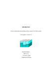
Figure 1.1 illustrates the three dimensional (3-D) block model (a.k.a. voxel model) used in
GRABLOX. The rectangular main block representing the volume below the measurement
area is divided into smaller brick-like volume elements. Each minor block is assigned
constant density value, ρijk. The gravity field is then computed as the superposition (sum) of
all the minor blocks using equation (4). For more information about 3-D block models,
please, see the documentation of the BLOXER program, which can be used to visualize and
to edit the 3-D block models.
Figure 1.1 Block model of size dX × dY × dZ (distance units) divided into
N = nx × ny × nz minor blocks of size dx × dy × dz (distance units). The model is
aligned with the (geographical) coordinate system.
GRABLOX2 can be used for both forward and inverse modelling (inversion). Gravity field
(gz) can be modelled with or without the vertical gravity gradient (gzz) or any combination of
the six gravity tensor components (gxx, gxy, gxz gyy, gyz, and gzz) used in Bell FTG system, or the
curvature component (guv = (gxx-gyy)/2) used in Falcon AGG system. The inversion method
optimizes the density of the blocks so that the difference between the measured and the
computed gravity (and gradient) data gets minimised. The optimization is based on linearised
inversion. The unconstrained inversion uses singular value decomposition (SVD) with
adaptive damping. The constrained inversion utilizes Occam's method where the roughness of
the model is minimised together with data misfit. The coefficients of the base anomaly, which
is represented by a second degree polynomial, can be optimised separately for the gravity and
gradient data. Density of the blocks can be fixed (and weighted) based on a priori information
5
(e.g., petrophysical or drill-hole data). Gradient data can be used together with gravity data in
the inversion, but gradient data cannot be inverted alone. After density inversion the
distribution of the density variations inside the resulting block model can be used in
geological interpretation.
1.1
About this version
GRABLOX2 has limited abilities for model maintenance. BLOXER is a separate, free
computer program that can be used for more enhanced model editing and visualization
(https://wiki.oulu.fi/x/eYU7AQ). BLOXER can be used, for example, to import a priori
density and topographic data into the model, export density values along vertical crosssections of the model, and to interactively edit density, fix/free and hidden/visible status of the
blocks. For even more advanced visualization of the 3D density models Golden Software's
Voxler is highly recommended.
GRABLOX2 cannot be used to optimize the height of the blocks. To perform two-layer
inversion for sediment and soil thickness, please, use the older GRABLOX version 1.7
(https://wiki.oulu.fi/x/EoU7AQ).
The 64 bit version of GRABLOX2 now contains OpenMP parallelisations that require the
presence of Libiomp5md.dll dynamic link library.
6
2. Installing the program
GRABLOX2 can be run on a PC with Microsoft Windows operating system and a graphics
display with a screen size of at least 1280  1024 pixels. In forward modelling the computer
memory and CPU requirements are usually not critical factors, because the program uses
dynamic memory allocation and the computations are quite simple. However, models with
hundreds of thousands of elements may take several hours to compute even on a modern
computer. Likewise, inversion of block models with tens of thousands of elements may not be
practical because of the increased computation time.
The size of continuous memory (1 GB) that is allocated for the sensitivity matrix restricts the
usage of the 32 bit version. The 64 bit version of GRABLOX2 that can only be run under 64
bit Windows does not have this memory restriction. Furthermore, the 64 bit version uses
OpenMP parallelisations and therefore runs faster on modern PC's with multiple processor
cores.
GRABLOX2 has simple graphical user interface (GUI) that can be used to modify the
parameter values, to handle file input and output, and to visualize the gravity data and the
model. The user interface and graphics are based on the DISLIN graphics library
(http://www.dislin.de).
The program requires either the 32 bit stand-alone version GRABLOX2.EXE or the 64 bit
version GRABLOX64.EXE and the LIBIOMP5MD.DLL dynamic link library for OpenMP
parallel computations. The distribution file (GRABLOX2.ZIP) also contains a short
description file (_README.TXT), user's manual (GRABLOX2_MANU.PDF) in PDF
format, and some example data (*.DAT & *.GAT) and model files (*.INP & *.BLX).
To install the program simply decompress the distribution ZIP file somewhere on a hard disk
and a new folder GRABLOX2 appears. When running the program over local network, one
should provide the network drive with a logical drive letter (e.g., Explorer/Tools/ Map
network drive…).
7
3. Getting started
After startup the program shows a standard file selection dialog, which is used to provide the
name of the input model file (*.INP). If the user cancels the file selection operation the
GRABLOX2.INP file will be used. If this file does not exist default parameters are used and
the file will be created automatically. The parameters of individual blocks are read from a
separate *.BLX file. Before the user interface is built up, the program reads graph parameters
from the GRABLOX2.DIS file. If this file does not exist default parameters are used and the
file is created automatically. The program runs in two windows: 1) the console (shell)
window and 2) the graphical user interface (GUI) window. The console window provides
runtime information about the current status of the program. The information appearing on the
console window is also stored in a log file (GRABLOX2.LOG).
After the initial model and the system parameters have been defined the user interface shown
in Figs. 3.1 is build up and a density map of the top layer is shown (cf. Appendix A1). The
model can be visualised using Layers and Sections push buttons. Repetitive use of Layers and
Sections push buttons will show successive layers or sections. Crossing dir button swaps
between (West-East directed) X-sections and (South-North directed) Y-sections. The <-/->
button is used to reverse the direction of layer and section swapping.
Compute button is used to perform forward computation. Map data button plots the data as a
2-D coloured contour or image map along with a 3-D view of the model and a short
description on some parameters (see Appendix B1). If the computation of gravity gradients is
activate, Gravity/Gradient button swaps the map between the two data types and
Grad. component button swaps the map between the six tensor components. Profiles (and
Crossing dir) button will display a single X- or Y-directed (interpolated) profile across the
data area. Model and system parameters are changed using the text fields on the left control
panel. Update button must be used to validate the changes. The computational settings can be
changed using the items in the Gravity menu. Most of the controls on the right control panel
are inactive before measured data have not been read in. To learn more about data
interpretation, please, refer to chapters 5 and 6.
8
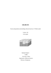
Figure 3.1. Grablox2 GUI with a layer
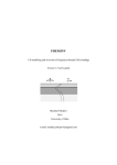
Figure 3.2. Image (pixel) map of the measured data.
10
Figure 3.2. Section view of the density model and the fit between measured and modelled data
11
4. The user interface
4.1
File menu
Open an existing model file (*.INP)
Read in gravity data for interpretation and comparison (*.DAT)
Read in regional data (stationary gravity field) (*.DAT)
Read in gravity gradient data (*.GAT)
Read in regional trend of gravity gradient (*.GAT)
Save the model into a file (*.INP)
Save the data (computed & measured) into a file (*.DAT)
Save the gradient data (computed & measured) into a file (*.GAT)
Save the results (description & data) into a file (*.OUT)
Read in new graph parameters from GRABLOX2.DIS
Save the graph in Adobe's Postscript format
Save the graph in Adobe's Encapsulated PS format
Save the graph in Adobe's (Acrobat) PDF format
Save the graph in Portable
Save the graph in Windows metafile format
Save the graph in GIF (graphics interchange format).
These menu items will bring up a standard file selection dialog that can be used to locate files
and provide the file name for open/save operations. The model parameters are saved in two
files: the first one (*.INP) defines files general properties and the second one (*.BLX) defines
the actual block model data. When saving the results, GRABLOX2 stores text information
into a *.OUT file. By default, gravity data are in a *.DAT file whereas gravity gradient data
are in a *.GAT file. All data files are stored in (ASCII/ISO8859) text format. Binary block
(*.BLX) files can be used to handle very large models more efficiently. See chapter 7 and the
BLOXER manual for more information about the block file format.
GRABLOX2 does not support direct printing. Instead, graphs need to be saved on a disk first
and then a suitable third party program (e.g., Adobe Acrobat Reader, Ghostview, Xnview,
etc.) can be used to print them or copy to clipboard. The graphs are saved in landscape A4
size as they appear on the screen. The GIF file is the only bitmap format (size 29702100
pixels). The Enhanced Postscript file does not include preview bitmap.
4.2
Gravity menu
Computed data is made as (synthetic) measured data
Computed data is made as (constant) regional field
Regional field is subtracted from measured data
Remove all information about measured data
Create a default model based on measured data
Define dimensions in meters, kilometers, feet or miles
Compute total field or anomalous field
Compute gz, gz & gzz or gz & 6 gradients & guv
Define background density mode
Define depth weighting mode
Define smoothing mode (on model borders)
Set additional computational options.
 CompMeas and Remove measured are useful when testing the program and using it for
educational purposes.
 CompRegi can be used to define a regional field using the current model. Alternatively,
one can use the Read regional data menu item.
 Subtract regional will remove the current regional field (if defined) and/or base anomaly
from the measured data. Removal of the regional trend reveals finer features in the mapped
data. The resulting dataset can be saved to disk for future use with the File/Save data item.
 Compute default is used to create an initial model. It is useful after new measured data has
been read in, because will give the super-block some reasonable coordinates based on the
data. If the data are regularly gridded the model is also discretised automatically, i.e., the
model is divided into minor-blocks that are positioned below the data points (z coordinates
also). When dealing with irregularly sampled data the user should perform the
discretization manually. Note that 2-D surface data and profile data are handled differently
and profiles that are not aligned with coordinate axes are not supported.
13
 When GRABLOX2 reads in data it does not know the units of the coordinates and
distances. The Scale unit item defines the actual volume of the block model, and hence, the
correct amplitude of gravity effect. Therefore, after reading in the data the user should
supply correct scale (meters, kilometers, or miles) before continuing with the modelling or
interpretation.
 The computed gravity field (gc) is the sum of 1) the gravity effect of the model (gm), 2) the
user defined base anomaly (gb) and 3) external regional field (gr)
gc = gm + gb + gr .
(6)
If regional field (gr) has been defined the Gravity field item can be used to include and
exclude the regional field to give either the total field or the anomalous field. The base
anomaly (gb) is always added to the computed response.
 Computation defines the three modes of the gravity computation:
1. The traditional gravity effect, i.e., the vertical component of the gravity field (Gz)
2. The gravity effect and the vertical gravity gradient (gz & gzz)
3. The gravity effect and the full gravity tensor, i.e., the six gradient components.
Note that this menu item cannot be used after measured data (gravity and gradient) has been
read in – the data itself defines the components that are going to be computed.
 Background defines the three modes of background density:
1. Normally, the background density has a constant value defined by the Bg dens field on
the left control panel. In this case, the background density is subtracted from the density
values of each minor block. Thus, if the density of the block is equal to the background
value it has no effect in the computed gravity anomaly.
2. In large-scale crustal studies the background density value can be defined as a function
of depth using the mean density of each layer. In this case, the mean density is
subtracted from the density of each minor block. This method is useful in large-scale
studies and when the density is assumed to increase downwards.
3. The background density can also be defined as the mean density of all the model blocks.
This method allows a simple way to define floating background value. If the density
increases downwards this method is not as good as the second one.
14
The purpose of the background density is to remove (or reduce) the effect of the four sides of
the main block especially when the model deals with absolute density values. If the contrast
between the mean density of the model and the background is large, the effects of the internal
density variations of the model will not be visible at all.
If the background density is zero, the inversion will resolve residual density where the mean
density of the modelled volume should be added to give geologically realistic density values.
When absolute density values, for example, from petrophysical samples are used to define the
initial model, the background value cannot be zero anymore. In that case, the background
value should be set to the mean of the sample values or, as usual, to the density value used in
Bouguer and topographic corrections (e.g., 2670 kg/m3).
Depth weight defines three modes of depth weighting used in density inversion. Normally, the
near-surface blocks have much larger sensitivity than the deep blocks. Consequently, the
inversion will generate a model where the masses are concentrated close to the surface, which
is likely to be geologically unrealistic. Depth weighting will place the mass distributions at
their "correct" depth by enhancing the importance and sensitivity of the blocks as a function
of depth. The depth weighting is discussed more in chapter 5.3.
The Gravity options sub menu contains following items:
 Autosave on/off enables and disables saving the model and data between each inverse
iteration. Since the inversion of large models is usually made overnight, this allows to see
how the model evolves in the inversion and to start the inversion again from any previous
model.
 Roughness on/off enables and disables the use of discontinuity information in the Occam
inversion. The discontinuity information is stored in the model file as a second parameter
with the help of the BLOXER program. If the model file does not contain discontinuity
parameter, this menu item will be inactive. See chapter 5.5 for more information.
 Laplacian on/off imposes Laplace's condition on the diagonal elements of computed
gravity gradients, gxx+gyy+gzz= 0. This option is used mainly for testing purposes.
 Inversion on/off enables and disables inversion and defines whether or not the sensitivity
matrix (Jacobian) will be computed automatically during forward computation when data
have been read in. For example, when CompMeas item is used to set computed
15
(synthetic) data to measured data, inversion (and related menus and controls) is not enabled
until it is manually enabled with this menu item. Note that when actual measured data is
read in, the inversion is enabled by default. However, if the model is very large the
program may be unable to allocate memory for the Jacobian. In this case GRABLOX2
disables the inversion and computes only the forward solution. After a new model with
smaller amount of elements has been defined this menu item can be used to enable the
inversion again.
 Gradient weights item provides a quick way to set the global weights for each gravity
gradient (tensor) component. Alternatively, one needs to edit the G-scale parameter for
each gradient component manually.
 Rotate gradient data is used to rotate the measured gravity gradient data horizontally, i.e.,
to perform tensor rotation around vertical z-axis. If the measurement lines are not aligned
with the geographical coordinate axes, it is advantageous to rotate the data coordinates so
that the model will be aligned with the data. However, airborne gravity gradient data (e.g.,
AirFTG®) is normally aligned with geographical coordinate axes and, therefore, tensor
rotation must be performed to adjust the tensor data accordingly. Note that tensor rotation
is different from coordinate rotation and that the vertical gradient (gzz) is not affected by
the horizontal rotation. Also note that currently GRABLOX2 does not support rotation of
data coordinates  that must be made using some third-party (spreadsheet) program.
4.3
Edit menu
Use either equal-height or increasing height blocks
Define min & max parameter value (and colour scale)
Set fix/free/hidden status of the blocks per layer
Set the density of the blocks per layer
Add margin blocks around the main block
Remove the outermost margin area
Define parameter labels shown in the graphs
Change the colour scale
Set view related settings.
 Although the xyz dimensions of the blocks can vary, all blocks have equal size by default.
In the alternative block type (Block type 2) the height of the blocks will systematically
16
increase downwards by the value of the topmost layer of blocks. For example, layer
thickness increases as 100, 200, 300, 400, 500 m giving depths 0, 100, 300, 600, 1000,
1500 m. The alternative block sizing thus reduces the resolution at the bottom but helps
decreasing the total number of blocks. Note that block type cannot be changed if the Shift
only editing mode is active (the second item in left control panel).
 Min/Max values item changes the limiting density values on the colour scale (below the
layers or sections view) and determines the absolute minimum and maximum density
values used in the inversion. These values also determine the maximum parameter steps in
SVD based inversion.
Note about the input dialogs: The parameter values are passed to the program via a text
string using a simple input dialog that appears on the display. The dialog does not contain
normal Cancel button. Therefore, to cancel the input operation one should close the dialog
with force (pressing the cross icon at the top-right corner) or provide an empty input string.
This rule applies to all other similar input dialogs.
 Layer-wise fix/free option allows setting the fix/free status (weights) and the visible/hidden
status of the blocks of each layer manually. Weights have integer values that range
between -101 and 100. Zero weight will fix the density of the block during inversion.
Weight equal to 1 and 100 make the density fully free and values ranging between 2 and
99 provide decreasing weight so that 2 is almost fully fixed and 99 is almost fully free.
Negative weight value will set the block hidden (the block will still carry the value of the
weight). Note that computationally, hidden block has density that is equal to the
background density. Hidden blocks are not drawn in layer and section views. See chapter
5.2 for more information about the fix/free status.
 Layer-wise reset option allows setting the density value of the blocks for each layer
manually. Fixed and hidden blocks are not affected.
 Add margins & Del margins can be used to add a single row/column of blocks horizontally
around the whole block model at once. Margins are important when interpreting gravity
gradient data, because they can be used to move the edge effects (due to the density
contrast between the block and the background) outside from the computation area. When
adding margins an input dialog appears and the user is asked to provide the width of the
margin blocks.
17
 Labels either removes the layer and section labels totally, or shows the numeric value of
the density, block height, block depth, fix/free status (weights), or the discontinuity (if
available).
 Color scale item is used to choose between normal rainbow scale, inverted rainbow scale,
normal grayscale, inverted grayscale and a special (seismic/temperature) red-white scale.
The Edit options submenu contains following items:
 Show/Hide grid can be used to clarify the contour/image maps as well as the layer and
section graphs.
 Contour/Image item swaps the display mode of gravity data between a contour map and an
image map where data are plotted as coloured rectangles. Contour plots are smoother but
more time consuming if there are lots of data points. Highly irregularly spaced data should
be as an image map because the interpolation can create artifacts.
 Show/Hide regional item enables/disables plotting the regional field or base anomaly.
When the regional field is not shown one can swap between computed and measured data
map to see the visual difference between them more easily.
 Show/Hide difference enables/disables plotting the difference between computed and
measured data as a map. When the difference is not shown one can swap between
computed and measured data map to better see the visual difference between them.
 Swap map area changes the limits of the data and layer maps so that they are either based
on the model area or the data area. If wide margins have been added to the model, this
option allows the user to focus either on the model area or the data area.
 Difference abs/% item defines the difference between the computed and measured data
either as absolute difference (data units) or as relative error (in percents). The relative error
is computed with respect to the (max-min) variation of the measured data.
18
4.4
Knots menu
Knots are a set of manually defined gravity points which can be used to represent the regional
field. This representation is made either by 2D interpolation or the base anomaly is optimised
on the knots instead of the gravity data. Knots are not used with gravity gradient data. Knots
are created and edited interactively on the profile response view. Their location can be edited
interactively on map views as well, but their level (gravity value) is defined by given value.
Knots are shown as crosses and circles on profile views and data maps, respectively.
Add knots on the current profile section
Edit knots on the current profile
Delete knots from the current profile
Interpolate a regional field through the knot points
Shift the knots on the level of the current regional field
The interpolation of the regional field (Knots->Regional) is made using a simple inverse
distance weighting. The idea is to add few sparsely spaced knots (minimum is 5 knot points)
on few sparsely spaced profile lines. These knots define a set of points through which the
regional field is then interpolated. The interpolated regional field replaces any separately
defined regional field read from a file. The base anomaly (defined by the coefficients of a
second degree polynomial) is still added to the computed regional field as usual.
If a user defined regional field and/or a base anomaly already exists, the Regional->knots
option allows shifting all current knot points on the level of the regional field. Again, a simple
inverse distance weighting scheme is used. This option is useful after the knot locations have
been added on the map view, because it provides a method to give the knots good initial
values that can then be edited in profile views.
Adding and editing of knots is also possible using the buttons at the bottom of the left control
panel of the GUI window. Please, see chapter 6.6 for more information on the knots.
4.5
Exit menu
Widescreen item is used to restart the GUI so that it fits the (old) 4:3 displays or (modern)
widescreen and laptop displays better. When entering widescreen mode the user needs to
provide a value for width/height ratio that is normally between 0.7 and 0.8.
19
Exit item is used to confirm the exit operation. On exit the user is given an opportunity to save
the current model and the results, provided that exit is made without an error condition. On
exit, the program first asks the name for the model files (*.INP & *.BLX) and then the name
of the results file (*.OUT). If the user cancels the save operation after choosing to save the
model or results, the default filename GRABLOX2.* will be used.
Errors that are encountered before the GUI starts up are reported in the GRABLOX2.ERR
file. When operating in GUI mode, run-time errors arising from illegal parameter values are
displayed on the screen. Some errors, however, cannot be traced and given an explanation.
The most typical problem is perhaps a corrupted GRABLOX2.DIS file that prevents the
program to start up properly. This problem can be circumvented simply by deleting the *.DIS
file. A missing or incorrectly named *.BLX file can also cause troubles. Please, note that most
messages that appear on the console window are stored also into a run-time log file
GRABLOX2.LOG. This file is written over when the program is restarted.
4.5
Left control panel
Update button is used (and must be used) to validate the changes made to the parameter text
fields. Once the Update button is pressed, the parameters defining the position, size, and
discretization of the block model are read in, checked for erroneous values and the old values
are replaced with the new ones.
The use of Update button invalidates existing computed results and a new forward
computation is needed.
The list widget below the Update button defines how the block parameters will be affected
when the Update button is pressed.
1. Shift only mode updates only the xyz position of the whole block model. The size and
the discretization of the main block cannot be changed in Shift only mode. This is the
default mode and it is purpose is to protect the model from accidental changes.
2. Ignore mode allows easy redefining of the size and discretization of the main block. As
the name implies, the existing relationship between the position and the density of the
blocks is ignored totally. The density of an arbitrary block p(i,j,k) remains the same but
it will most likely move to a totally different position inside the model if the
discretization (indexing) changes.
20
3. Preserve mode uses simple 3-D nearest neighbour
interpolation to define new density values of the blocks
when the model is resized, re-discretised, or repositioned.
For example, if the position of the main block is shifted,
the anomalous target remains more or less at the same
geographic position, but its relative position (indexing)
inside the main block will change. Note that 3-D
interpolation of densely discretised and large models can
be very time-consuming.
The following text fields define the position, size and
discretization of the main block:
1.
X position (easting) of the SW corner of the main block
2.
Y position (northing) of the SW corner of the block
3.
Z position (depth to the top) of the main block
4.
X size of the main block (in EW direction)
5.
Y size of the main block (in NS direction)
6.
Z size or height of the main block (downwards)
7.
X discretization (number of blocks) in EW-direction
8.
Y discretization (number of blocks) in NS-direction
9.
Z discretization (number of blocks) in vertical direction.
In GRABLOX2 the true dimensions (distances) of the block
model (and computation grid) are defined using the
Gravity/Scale unit
menu
item.
The
given
rectangular
coordinates do not need to be actual geographic map coordinates. To be able to better model
geological strike directions, for example, the data and the model should be defined using
rotated coordinates.
The next two text fields define two density parameters:
1.
Bg dens defines the user defined background density value, 0 (g/cm3)
2.
Param defines the default density value used to reset the model into, 1 (g/cm3).
21
Note about density units: In GRABLOX2 the density is defined in units [g/cm3]. Use the
BLOXER program to modify density values if required. For example, divide by 1000
(actually, multiply with 0,001) if densities are given as kg/m3.
Reset dens button resets the density of the whole model to the value defined in Param text
field. Note that fixed and hidden blocks are protected and will not be affected.
The gravity field [mgal] and gravity gradients [Eo] are always computed using some density
contrast  = i - 0 [g/cm3], that is to say, the difference between the density of the blocks
(i ) and the background density (0). The method used to define the background density is
chosen using the Gravity/Background menu item. When Given value mode is active, the value
of background density provided in Bg dens field will be subtracted from the density values of
each minor block. Note that density values can be absolute (background density and density
range is based on petrophysical data, for example, 0= 2,7 g/cm3 and 2,0 <  < 3,6 g/cm3) or
relative (background value is zero or arbitrary, e.g. -0,6 <  < +1,2 g/cm3). The computed
gravity results will be exactly the same if the density contrasts with respect to the value of
background value are the same.
In forward computations the rectangular computation grid is defined by the seven text fields
below Reset dens button:
1. X-step:
spatial step between computation points in x direction, dx
2. Y-step:
spatial step between computation points in y direction, dy
3. X-start:
x coordinate (easting) of the grid start position, x1
4. Y-start:
y coordinate (northing) of the grid start position, y1
5. X-end:
x coordinate (easting) of the grid end position, x2
6. Y-end:
y coordinate (northing) of the grid end position, y2
7. Z-level:
constant z level (height or elevation) of the computation grid, zh.
If the width of the computation grid is zero (e.g., x1 = x2 or y1= y2) the computations are
made along a single profile that extends from (x1, y1) to (x2, y2) and X-step is used as a
distance step between the computation points along the profile. In this case the profile is
aligned either with x axis (y1= y2) or y axis (x1 = x2). A more general (azimuthal) profile
from (x1, y1) to (x2, y2) can be defined, if Y-step is set equal to zero (dy = 0). In this case the
X-step is used as a true distance between the points along the slanted profile. Naturally,
22
profile data can be plotted only as a profile plot (no contour or image maps). However, in this
case the data are drawn exactly without any interpolations. Also note that depending on the
current status of data extent (defined by Edit/Edit options/Swap map area menu item) the
layer view shows only the part of the model below the profile.
Note about Z-level and X- and Y-steps: The abovementioned values are defined separately for
gravity and gravity gradient data. The Gravity/Gradient button in the right control panel is
used to swap the currently active data component. The information text in the graph shows the
current data mode.
Measured data are assumed to be irregularly spaced. The computations are always made at the
actual data locations (x,y,z). Therefore, grid start and end positions are inactive after measured
data have been read in. Moreover, when data has been read in X-step and Y-step define grid
spacing used in contour and image maps. When the data are irregularly spaced, x and y steps
should be edited manually to reduce possible contouring artifacts.
Note about data elevation: The z coordinates (elevation or topography) of the measured data
are used only if they are provided with the data AND the Z-level is equal to the top of the
main block (Z-level = Z-posit.). Otherwise, the response will be computed at the constant
elevation defined by the Z-level. This method allows inspecting the effect of height in gravity
computations. To compute the gravity field on the surface of the block model, t must set the
Z-level very close to the Z-posit value (but do not make them equal).
The pull-down list widget and the text field Value below it are used to define the coefficients
of a second degree polynomial used for computational base anomaly of a form:
gb(x,y) = A + B(x-x0) + C(y-y0) + D(x-x0)2 + E(y-y0)2 +F(x-x0)×(y-y0) ,
(7)
where x0 and y0 define the shifted origin for the base function. By default the origin (x0, y0) is
located at the middle of the main block. Because the amplitude changes of gravity anomalies
are small compared to the distances, the values of C and D are scaled (multiplied) by 1000
and the values of E and F are scaled by million. Thus, if dimensions are defined in meters, the
linear and second order coefficients are defined as mgal/km and mgal/km2, respectively. The
base anomaly is always added to the computed gravity anomaly even if external regional field
has been read in.
23
Note about the base anomaly: The base anomaly is defined separately for the gravity data (gz)
and each gravity gradient component (gxx, gxy, gxz, gyy, gyz, gzz and gzz) depending on the current
active data component defined by Gravity/Gradient button. In other words, when gravity data
is active (is currently mapped or plotted) the coefficients are related to the base anomaly of
the gravity data and when gradient data is active the coefficients are related to that.
Update base button at the bottom of the left control panel is used to update the changes made
to the base level immediately without the need to do full forward computation. Reset base
button is used to reset (null) the first and second order coefficients of the base anomaly of the
currently active data component. In other words, Reset base resets all other coefficients but
the level (A).
Optimize base to knots check box changes the way base anomaly inversion is made is inactive
if there are no knot points. Knots are used to define a user defined regional field by 2D
interpolation. Knots can also be used to define a set of gravity data points upon which the
base anomaly will be optimised. Add knots and Edit knots buttons enable interactive editing
mode where knots can be inserted into map and profile views. The level of existing knots can
be edited only in profile view.
4.6
Right control panel
The Compute button is used to perform the forward computation using the current values of
the model and system parameters. The Optimize push button is used to start the inversion.
Note that depending on the total number of minor blocks and the amount of computation
points, the inversion can take a considerable amount of time.
The list widget below the Optimize button defines the three inversion modes:
1. Base optimizes the coefficients of the base anomaly,
2. Density optimizes the density of the free minor blocks using SVD based method
3. Occam density optimizes the density of the free minor blocks using Occam's method,
where both the data misfit (difference between the measured data and the computed
response) and the model roughness are minimised.
The second list widget defines which coefficients or a combination of coefficients of the base
anomaly is going to be optimised when Base optimisation is performed. Note that in Occam
density inversion the linear coefficients (A, B, or C or A, B and C) of the base anomaly of the
24
gravity data (not the gradient data) can be optimised together with density values. One must
remember to select None if one does not want the base anomaly to be optimised together with
density. Note that in practice combined inversion of base anomaly and block parameters
requires that some density values are fixed based on additional a priori information.
The optimization of the base anomaly is performed either on the gravity data or gravity
gradient data depending on the current status of the mapped data defined by the
Gravity/Gradient button.
The following five text fields define some inversion related
options. See chapter 6 for more information about the
abovementioned inversion options.
1. Iters defines the number of iterations made during one
inversion run.
2. Thres % defines the strength of damping in SVD based
inversion. Normally, the threshold should be at the level
of the smallest singular values that are still informative.
The smaller the threshold value is the weaker is the
damping. Note that the value is actually multiplied by
100. Thus, the default value 0.01 (%) is actually 0.0001,
and all singular values < max/105, where max is the
maximum singular value, will be damped.
3. F-option provides a numerical (real) value for an
additional parameter to the inversion. Its role depends
on the selected inversion mode. In SVD based inversion
it determines the maximum step controlling the
convergence. In Occam inversion it is used as a
Lagrange multiplier or scaler controlling data fit vs.
model smoothness.
4. I-option provides a numerical (integer) value for an
additional parameter to the inversion. Its role depends
on the inversion mode  in Occam inversion it is used to
control the rigidity of fixed blocks whereas in base
25
inversion it is used to shift the fit towards the bottom or the top of the gravity or
gradient anomaly.
5. W-norm increases or decreases the depth weighting as a function of depth. The value
should be changed from the default value 1,0 only if the inversion results seem to
overestimate or underestimate the density values at the deep parts of the model. For
example, W-norm value 2,0 enforces twice as strong depth weight at the bottom of the
model and a value 0,5 gives only half as strong depth weighting.
6. G-scale defines global data weight for individual data components when gravity data
and gradient data are optimised together. Depending on the current status of the mapped
data (Gravity/Gradient button) the weight is related to gravity data or one of the gravity
gradient components. The value should be changed from the default value only if the
inversion seems to emphasize or de-emphasize one of the data components too much.
For example, decreasing the global weight of Gxy gradient component to 0,1 will make
the corresponding data error 10 times smaller and, consequently, gives that data
component less importance in the inversion.
The next three push buttons are used to show and define the current gravity data.
 Map data button shows the gravity data as a coloured 2-D map. If measured data has
been defined, repetitive use of the Map data button will swap the view between the
computed and measured data, the data error (difference between measured and
computed data) and the regional or base response data. The map type can be changed
between contour or image map using Contour/Image item in the Edit/Options submenu.
Plotting of data error and regional field can be omitted using Show/Hide difference and
Show/Hide regional items in the Edit/Options submenu.
 Gravity/Gradient button swaps the current data component between gravity field and
gravity gradient. The item is active only if gradient computation has been enabled
(using Gravity/Computation menu item).
 Grad comp. button swaps the current data between different gradient components when
full gravity tensor data is being computed. The item is active only if gradient
computation has been enabled (using Gravity/Computation menu item).
Layr/Sexn text field shows the index number of the current layer or section when the model is
being visualised (see the meaning of the buttons below). It is possible to jump from one layer
26
or section to another by first giving a new value for the index number manually and then
pressing the Layers or Sections button.
 Layers button is used to show the density values across a horizontal layer.
 Sections button is used to show the density values across a vertical cross-section.
 Profiles button is used to show the computed and measured data and the regional/base
anomaly as XY graphs over the data area. The data is either gravity or gravity gradient
depending on the status of current map defined by the Gravity/Gradient button.
 Crossing dir button is used to change the direction of the sections views and data
profiles between (vertical) SN and (horizontal) WE directions.
 <-/-> button is used to change the rotation direction of contours/image maps, layers,
sections and profiles when the corresponding buttons are pressed.
When the Layers, Sections, and Profiles buttons are pressed multiple times the current layer,
section or profile is rotated, that is to say it changes to the next or previous one depending on
the direction defined <-/-> button. After the last (or first) layer, section or profile the view
jumps back to the first (or last) one. One can jump directly into a desired layer or section by
first providing the index number on the Layer/Sexn text field and then pressing the
corresponding push button.
Normally, section view shows only a vertical cross-section of the model and profile view
shows the profile response. Activating the Profile+Section changes the graphs so that the
profile response is shown on top of the model cross-section. In this case, pressing the Section
of Profile buttons will continue swapping the profile or the section while the other view
(section or profile) remains the same. The Align prof/section button is used to align the profile
and section views. If profile view was changed the index number of the section will changed
so that it will show the model below the profile. Likewise, if section view was changed the
profile closest to the section will be shown in the upper graph.
If the data covers a two-dimensional area it assumed to be irregularly sampled and the profile
graphs show the data interpolated along (imaginary) x or y directed profiles, the interval of
which are based on values of the X-step and Y-step text fields in the left control panel. This
means that the profile response displays the original data only if the data are regularly gridded
and the steps are equal to that of the data. If the data are highly irregular, the DISLIN
27
contouring algorithm used in GRABLOX2 may not work well and the profile response shows
up incorrectly. Some improvement can be made by changing the data representation from a
contour map to an image map using the Contour/Image item in Edit/Options submenu.
Alternatively, the data could be mapped on a regular grid beforehand using some third party
interpolation software (e.g. Golden Software Surfer or Geosoft Oasis Montaj).
GRABLOX2 suits also 2.5-D interpretation of single profile data. In this case, the data should
be aligned with either the x or y axis so that the Gravity/Compute default can be used to
generate a proper initial model automatically. Consequently, if the profile is aligned with y
axis, the model will be discretised along the x and z directions, the y discretization (Y-divis.) is
set equal to one, and the strike length (Y-size) is made so large that the model appears to be
two-dimensional. Although it is possible to compute the forward response along general
profiles that are not in x or y direction, a 2.5D model cannot be constructed properly, since the
model is always discretised along x and y axes. Note that 2.5-D inversion methodology has
not been tested thoroughly. It is likely that the depth weighting needs to be redefined for
models having elongated strike length.
Normally, the vertical depth axis is plotted in 1:1 scale with horizontal axes in X and Ysection views. Vert. scale slide control can be used to stretch or squeeze the depth axis. It is
useful if the height of the model is considerably smaller than its horizontal dimensions. The
other three slide controls (Horiz. rotation, Vert. rotation and Rel. distance) are used to change
the view point of the small 3-D model view next the main graph.
The Update graph button is used to validate the changes made to the slide controls and to
redraw the current graph.
28
5. Inversion modes
The three inversion modes are:
1. Base
SVD based optimisation of the base anomaly (coefficients A-E)
2. Density
SVD based (unconstrained) optimization of the density
3. Occam
(constrained) Occam inversion of the density.
Density values are limited by the minimum (Min) and maximum (Max) values of the colour
scale below the Layer and Section graphs. The limit values are set using the Min/Max values
item in the Edit menu.
5.1
Regional field
The measured gravity field is always affected by mass distributions both near to and far away
from the study area. The purpose of the regional field in GRABLOX2 is to account for (and
subtract) the gravity effect of all those masses that are located around and below the volume
of the 3D super-block. Although the regional field can be defined almost arbitrarily, the
important thing is not to remove any gravity effects that might be explained by density
variations inside the volume of the 3D block model.
The three ways to define the regional field in GRABLOX2 are:
1.
User-defined base anomaly is defined by a second degree polynomial,
2.
Regional field is read in together with the measured data (Read data), or
3.
Regional field is read in from a separate file (Read regional).
The choice of the regional field is one of the most important factors of successful gravity
interpretation. Best results are obtained if the regional field is interpreted separately using a
large regional model and gravity data that extends 25 times farther than the actual
interpretation model of the study area. The block size of the regional model can be 210 times
larger (horizontally and vertically) than what will be used in local modelling. The
discretization of the local and regional models should be set so that the block boundaries
(sides and bottom) of the local model fit the discretization of the regional model. Once the
regional-scale inversion has been made and an acceptable model has been found, the volume
of the local study area is removed (hidden) from the regional model (with BLOXER) and the
regional, large-scale gravity anomalies of the surroundings are computed at the data locations
of the local study area and saved into file. Alternatively, surface fitting or low-pass filtering
29
(e.g., Surfer, Geosoft, Fourpot) can be used to define the regional trend of the gravity
anomaly. These methods, however, are somewhat vague, because they do not take into
account the real physics and the depth extent of the targets.
The regional trend of the gravity data can be defined using the optimization of the parameters
of the base anomaly. Although a second degree polynomial used in GRABLOX2 cannot
describe as complicated regional effects as external files, it is often a good approximation to
the regional gravity effects. Also note that the base anomaly is useful also if the data and/or
regional field for some reason are not in level with the measured gravity data.
Note about the base anomaly: Base anomaly is always added to the computed response.
Nonetheless, it can be used together with the user defined regional field also. Therefore,
optimization of the coefficients of the base anomaly provides a method to adjust the first and
second degree behaviour of the regional field. Furthermore, in Occam inversion the base level
and/or linear trend (A+Bx+Cy) of the base anomaly of the gravity field can be optimised
together with the density values (although this can be ambiguous).
The Gravity/Subtract regional item can be used to remove the regional field from the
measured data and the new data can be saved into a file (File/Save data). Theoretically, there
should not be any difference if the inversion is made using total field or anomalous field.
However, if the regional trend has been removed from the original data, the visual inspection
of the data and fit between measured and computed data is often much easier. Moreover, the
absolute minimum and maximum values and the dynamic range of the data will be different.
As a consequence, inversion uses different data weighting and is likely to yield slightly
different results. The users are advised to work with anomalous field if a very strong regional
trend is included into the original gravity data.
5.2
Fix/free status
The fix/free status defines whether the block is included into the inversion (optimization) or
not. In GRABLOX2 it serves also as weight factor defining relative importance of the fixed
density values. The weight factor is utilised only in Occam inversion. The fix/free value is
zero (0) for a totally fixed block (not optimised at all), and either one (1) or one hundred (100)
for a totally free block. Fix/free values ranging from 2 to 99 define variable weights. Note that
in a *.BLX file, the fix/free status is stored as an integer value.
30
The Layerwise fix/free item can be used to manually set a constant fix/free value for each
layer. Note that it can also be used to set the hidden/visible status of the blocks per each layer.
Hidden blocks are removed totally from the computation. As such they represent the density
of the background medium. For more advanced editing of the fix/free and hidden/visible
status one should use the BLOXER program.
5.3
Depth weighting
Normally unconstrained (and un-weighted) gravity inversion tends to put the excess mass
mainly in (or remove the missing mass mainly from) the uppermost blocks, because their
sensitivity is much greater than that of the deeper blocks. Consequently, the resulting inverse
model is not likely to be geologically realistic. The concept of depth weighting (Li and
Oldenburg, 1996 and 1998) tries to overcome this problem. Basically the idea is to multiply
the elements of the sensitivity matrix and the difference vector with depth dependent function
of form
wd = (z+z0)a ,
(8)
where z is the depth of a block from the top of the main block, z0 is a scaling value that
depends on the size of the blocks, and a is an exponent that depends on the geometric form of
the potential field. The gravity field has 1/r2 dependency on the distance from the source.
However, experimental value a = 1 gives better convergence in 3-D gravity inversion.
One problem with depth weighting is that it does not take a priori data into account and
possible near surface mass distributions will get incorrectly positioned. To circumvent these
problems GRABLOX2 has an option to automatically relax the depth weighting based on the
value of the current RMS error. When the RMS error decreases during the inversion so does
the depth weighting until it disappears when RMS reaches level of 0,2 %. In practice,
however, full depth weighting should be used and the other two options (relaxed or discarded)
should be used just to test the effect of depth weighting.
The status of the current depth weighting method can be derived from the last line of the
information text next to the model and response graphs. After the inversion mode (Base
optimization, SVD inversion, Occam inversion) the first integer number defines the depth
weighting mode (0= none, 1= relaxed, 2= full). The second number shows whether or not the
31
automatic model saving is active or not (0= no, 1= yes). If the model file includes
discontinuity information the third number would indicate if it is active or not (0= no, 1= yes).
5.4
Normal SVD based inversion
Base and Density inversion modes are based on a linearised inversion scheme similar to that
defined in Jupp and Vozoff (1975) and Hohmann and Raiche (1988). The optimization uses
singular value decomposition (SVD) and adaptive damping method defined in Pirttijärvi
(2003). For the sake of clarity, the basics of the linearised inversion method are discussed in
the following.
The objective of the numerical inversion is to minimize the difference or misfit (e = d-y)
between the measured data, d = (d1,d2,…,dM) and the computed response y = (y1,y2,…,yM).
Assuming an initial model with parameters p = p0 = (p1,p2,..pN), forward computation is made
to yield model vector y and the sensitivity or Jacobian matrix, A, the elements of which are
partial derivatives of the model data with respect to model parameters (Aij = yi,/pi). Thus,
the linearization of the problem leads to matrix equation
A · Δp = e .
(9)
Solution to Eq. (9) gives parameter update vector Δp, which is then used to give updated
parameter vector, p1 = p0 + Δp. The process is continued iteratively until desired number of
iterations has been made and/or the fit between the measured and computed data becomes
small enough. The root-mean-square (RMS) error is used as the measure of the data fit
√ ∑
(
) ,
(10)
where Δd = max(d)-min(d) is used to scale the data. The singular value decomposition (SVD)
of the Jacobian is (Press et al, 1988)
A = UVT,
(11)
where U and V are matrices that contain the data eigenvectors and data eigenvectors (T means
transpose operation) and  is a diagonal matrix that contains the singular values. Since both U
and V are orthogonal matrices, the solution to Eq. (9) is
32
Δp = VUT,
(12)
where the elements of the diagonal matrix are simply 1i. If some of the singular values
are very small the inverse problem becomes ill-posed. Therefore, stabilization or damping is
performed by adding a small value, so-called Marquart factor, , to the singular values giving
i+). In practice, the singular values are multiplied with damping factors (Hohmann and
Raiche, 1988)
 si4

ti   si4   4
 0

si   2
si   2
,
(13)
where si = i /max() are normalised singular values and  is the relative singular value
threshold. Thus, elements of  that correspond to very small singular values are removed
totally and the remaining values are damped so that they are never too small. The damping
diminishes the effect of small singular values and the threshold is used to control the strength
of damping.
Thres % field defines the minimum value of the relative singular value threshold. Normally, it
should be at the level of the smallest singular values that are still "informative". The threshold
should be changed only if the inversion becomes unstable. Larger threshold value forces
stronger damping, which suppresses the effect of small singular values and improves the
stability of the inversion. Note that the %-character is used just to remind that the value is
actually multiplied by 100. Thus, the default value 0.01 is actually 10-4.
F-option parameter defines the maximum parameter step for the adaptive damping (Pirttijärvi,
2003). Small value of F-option makes parameter steps smaller, increases the value of relative
singular value threshold and thus the damping, and (usually) makes the convergence slower.
Large value of F-option makes parameter steps bigger, reduces damping closer to that defined
by minimum singular value threshold, and thus increases the convergence. However, it may
also lead to unstable convergence. In practice, the F-option value should range between 10–
0,1 and the default value 1,0 provides relatively good convergence.
33
The numerical computation of the SVD is the most time-consuming part of the inversion. It
has approximately O3 dependence on the total number of minor blocks. Because SVD based
inversion can be time consuming, Occam methods that use iterative (conjugate gradients or
QR) solvers are preferred when the number of blocks is > 10000.
5.5
Occam inversion
The famous citation from Wilhelm of Occam (Ockham) from the 14.th century states: "Non
sunt multiplicanda entia praeter necessitatem", which translates "Plurality should not be
assumed without necessity" or "One should not complicate matters beyond what is
necessary". This so-called "Occam's razor" means that if two solutions are equally good the
one that is simpler should be preferred. In geophysical inversion practice Occam's method
means that in addition to minimizing the fit between the measured and computed data the
roughness of the model should be minimised also. In practice, Occam inversion will produce
smoother models because the neighbouring density values are used as constraints. As a
drawback, the models may not fit the data as well as the unconstrained (SVD) inversion.
However, the so-called Lagrange multiplier (provided via F-option parameter) can be used to
control the minimization of either the data error (fit) or model roughness (smoothness).
Occam density inversion mode optimizes the density of the free blocks. An important feature
of Occam inversion in practice is that if the densities of some blocks are fixed, Occam's
method will constrain the parameters of the surrounding blocks to fit those of the fixed
blocks. For example, petrophysical data can be used to constrain the density at the surface.
The ability to constrain the parameter values reveals another advantage of Occam's method.
The Occam inversion can create a smooth and continuous model, even if the measured data
are irregularly spaced and do not cover the whole model area. In such situations the normal
(unconstrained) SVD based inversion gets unstable and tends to generate very rugged (chessboard) structures.
The roughness, r, is defined as the difference between the density of a minor block from the
mean density of the surrounding blocks, r = p-p*. In practice, the roughness (or its reciprocal,
the smoothness) is incorporated into the Eq. (9) by adding the sensitivities of the roughness
(Bij = ri,/pi) and extending the data error vector with the model error e', which in general is
computed against some reference model, but in this case the null-model so that e' = r.
Occam's method leads to a new matrix equation
34
(A + B) · Δp = (e+e') .
(14)
where  is so-called Lagrange scaler (multiplier) that is used to emphasize either the fit
between the data or the smoothness of the model.
Since the number of data M is typically equal (or smaller) than the number of blocks in the
top layer, the dimension of the linear system increases quite drastically, NM ( N(M+N).
In this case the SVD would become too slow to be practical. Therefore, Occam inversion uses
either iterative conjugate gradient (CG) algorithm or QR decomposition (Householder
rotations) to solve the matrix system for the parameter steps. The CG solver is faster than QR
but it requires an additional matrix for the normal equations (ATA). Therefore, CG is used as a
default solver, but QR method is automatically chosen if memory cannot be allocated for the
normal equations.
In Occam density inversion the coefficients of the linear part of base anomaly (A+Bx+Cy) can
be optimised together with density values if the second scale widget in the right control panel
is set to appropriately (Base A, X-grad B, Y-grad C or Linear ABC). The second order
coefficients cannot be optimised because they would most probably remove (or add) excess
mass from the gravity anomaly itself.
F-option defines the Lagrange scaler (L = ) in the constrained Occam density inversion.
Lagrange scaler controls if the inversion should give more importance to minimizing the data
error instead of minimising the model roughness, or vice versa. Since both the data values and
the model parameters are normalised, the default value (L= 1.0), usually gives approximately
the same importance to the data and the model error. Increasing the Lagrange scaler (L> 1,0)
will emphasize the importance of model roughness and the inversion will create smoother
models with the expense of increased data misfit. Decreasing the Lagrange scaler (L<1,0) will
emphasize the data error and the inversion will create rougher models that fit the data better.
One should experiment with different values of the Lagrange scaler and decrease it during
successive iterations. When multiple iterations are made overnight, for example, automatic
Lagrange scaling can be activated by giving a negative value to the F-option parameter (e.g.,
L= -1,0). The automatic value of Lagrange scaler is based on the RMS-error and the given
value of F-option. The automatic value is always between abs(L) and abs(L)/10.
35
Note that the Occam inversion enforces smooth density variations. In real world the density
changes are much more abrupt. The Lagrange multiplier sets a global value for the desired
model roughness. The fix/free status and the discontinuity parameter provide means to define
local variations in the smoothness constraint. The fix/free status imposes certain kind of
rigidity around a fixed block. Additionally, discontinuity parameter can be used to define
discontinuous interfaces in the model, thus, allowing rapid changes between selected two (or
more) blocks.
G-scale parameter is used in Occam inversion as global data weight and it is defined
separately for the gravity and each gradient components. To change the current data
component one needs to use the Gravity/Gradient and Grad. component buttons. Increasing
the value of global data weight increases the importance of the current data set in the
inversion. On the contrary, decreasing the G-scale value decreases the importance of the data
component. The data set can be discarded totally by setting the value of the G-scale parameter
to zero. Note that currently the data cannot be given individual weights that would depend on
the measured data error, for example. This feature may be added in the future.
5.5.1
Discontinuity information
The objective of the discontinuity is to define interfaces across which the Occam method will
not continue the smoothing. Blocks that are marked with discontinuity information are not
added to the mean of the surrounding blocks when the roughness is computed in Occam's
method. In practice the discontinuity information is stored as a second parameter in the
*.BLX file with the help of the BLOXER program. The discontinuity is defined using a single
(real or integer) value that consists of the sum of following values:
0
1
2
4
8
16
32
64
fully continuous block (normal case)
fully discontinuous block (special case)
discontinuous towards positive x axis (north)
discontinuous towards negative x axis (south)
discontinuous towards positive y axis (east)
discontinuous towards negative y axis (west)
discontinuous towards positive z axis (down)
discontinuous towards negative z axis (up).
36
For example, value 126 (2+4+8+16+32+64) means that the block is discontinuous in all
directions, 30 (2+4+8+16) means that the block is horizontally discontinuous and vertically
continuous, whereas value 96 (32+64) means that the block is horizontally continuous and
vertically discontinuous. Likewise, value 2 means that the discontinuity interface is to the
eastern side of the block. Usually, in this case the block on the eastern side will have value 4
(discontinuity is on the western side of the block). Discontinuity is stored into the model
*.BLX files as the second parameter after the density. Discontinuity can be edited into the
model manually or imported like topography (surfaces, lines, points) using the BLOXER
program. The discontinuity information should be based on a priori information (or well
established assumption). Please, note that this method is still under development.
5.6
About computation time
The computation time depends directly on the number of blocks and the number of points
where the gravity field is to be computed. Computation of gravity gradients is slightly more
time consuming and each gradient component requires some additional time. As an example,
consider a model where the number of free blocks is N= 34308= 8160 and the number of
data points is M= 1020. On a PC with 3.2 GHz Intel i5-2500K CPU the forward computation
takes about 0,55 seconds using the 64 bit version of GRABLOX2on a 64 bit Window 7. As a
comparison, the computation took 0.76 seconds using the 32 bit version of GRABLOX2.
Although Occam inversion needs to solve much larger matrix system than the SVD, the use of
an iterative (CG or QR) solver makes the overall inverse computation much faster.
Considering the previous example where the dimension of the linear system is 9180 × 8160, a
single iteration took about 75 seconds to compute (64 bit version). Most of the time is spend
redefining the Jacobian, i.e., computing normal equations ATA. If there is not enough memory
to allocate the auxiliary ATA matrix, a QR solver is automatically used. In case of the 32 bit
version this typically happens when N>15.000. The QR algorithm is computationally more
time consuming than CG solver and, hence, it is used merely as an alternative solver. Because
of the slowness and the unconstrained nature the SVD inversion it should be avoided when a)
the dimension of the inverse problem is greater than 12000 × 2000, and/or b) some model
parameters are fixed based on a priori information. For comparison, a single iteration with the
SVD based inversion too about 13 minutes to compute in the example case (1020×8060).
37
6. Guidelines for gravity inversion
Numerical inversion of gravity data aims to obtain a model whose synthetic response fits the
measured gravity data (and gradient data, if available) with sufficient accuracy. GRABLOX2
is a relatively simple software tool that can be used to determine one or few possible solutions
to complicated 3-D gravity problems. The big problem, however, is the non-uniqueness of the
inverse solution. One should never consider the inversion results final - they only show
possible solutions. Combined geophysical and geological interpretation is always needed to
estimate the physical meaning of the inversion model and to decide whether or not the
solution is acceptable.
This chapter discusses the various steps needed for the gravity inversion based on a 3-D block
model and how they can be accomplished with GRABLOX2 and BLOXER. The reader
should note that this chapter applies to forward modelling also. Neither the actual combined
geological and geophysical interpretation nor the theory and applications of the gravity
method will be discussed.
6.1
Precautions
Preliminary inspection of the data is used to assess the data quality and sampling and to give
some insight to the relation between the gravity anomalies and geological structures.
Computer software such as ESRI ArcGIS, Golden Software Surfer or Geosoft/ Oasis Montaj
can be used to visualize the gravity, topography, and petrophysical data. Digital geological
maps are also useful in the visualization of gravity and petrophysical data.
Before inversion it is also necessary to estimate the dimension of the problem. Although
forward computation is quite fast, models with tens of thousands of blocks require lots of
computer resources. Nowadays, the amount of physical computer memory rarely hinders
forward computation, but it can easily prevent inversion.
6.2
Data preparation
First of all, one needs to define the gravity data for the inversion. In other words, one needs to
create a column formatted data file (*.DAT) and check its format, dimensions (m, km, ml or
ft), and units (mgal, Eo). The data can be evenly discretised or irregularly spaced, and it can
include topography or elevation values. Remember, however, that one must choose the study
area and the data sampling based on the practical limits of the inversion. For example,
38
inversion of 3030 data points using a 3-D block model with 10 layers leads to quite a
feasible problem of dimension MN = 900 data points  9000 blocks. Doubling the horizontal
discretisation to 6060 points will yield a problem of MN = 3600 data points  36000
blocks, which requires running the inversion overnight.
Pre-processing (filtering, levelling, corrections) should be made to the data beforehand.
Although it is not required, the gridded data should be stored as continuous lines of x
coordinate (from West to East) for each y coordinate (from South to North). If the data are
measured along lines that are not aligned with main geographical coordinate axes, the
coordinates should be rotated so that the new data area coincides with the coordinate axes of
the model. If the data coordinates cannot be rotated the model must be made larger than data
area and a certain amount of the blocks will be wasted in the corners of the model. In that
case, one can hide the blocks outside the data area with BLOXER program.
Note that data from a single profile can be interpreted using a 2.5-D model (see chapter 7.2).
In that case, the data should be defined so that the profile is aligned with the x axis or y axis
so that an initial 2.5D model perpendicular to the profile can be constructed (Compute default
menu item). Note, however, that it is possible to interpret single profile data using a fully 3D
block model, although that would be somewhat ambitious.
Secondly, one needs to define the regional field if such data are available. The regional field
can be included in the gravity data file or read from a separate file. In the both cases, the
regional data should have exactly the same x and y coordinates as the gravity data, although it
suffices in the latter case that the regional data have the same number of points as the gravity
data.
Thirdly, one needs to define the gravity gradient data if such data are available. The gradient
data are provided in a separate file, and need not have the same (x,y,z) coordinates or data
extent as the gravity data. The header of the file defines the order in which the gradient
(gravity tensor) components are stored in the file. The file can contain just one or several
gradient components. The diagonal elements (gxx, gyy and gzz) of the gravity tensor are usually
the most useful gradient components.
6.3
Preliminary operations
After starting up and after opening some previously defined model file (possibly a dummy file
if one cancels the file open procedure), the first thing is to read in the gravity data using the
39
Read data item in File menu. If regional gravity field is not included in the same data file it
can be read in using the Read regional data item. Likewise, gradient data is read in using the
Read gradient data item. The Map data and Profiles (and Crossing dir) buttons can now be
used to visualize the data as contour or image maps and profile sections. The
Gravity/Gradient button changes the current view between gravity and gravity gradient data.
The Grad component button changes the current view between different gradient components
(if available). Note that profile graphs are always interpolated from the (assumed) irregular
data.
At this point the user should check the dimensions and use the Gravity/Scale unit menu item
to choose between meters, kilometres or miles. This is an essential task for correct amplitude
of the gravity and gradient computations. In forward modelling one should also check the
Gravity/Computation menu item. The default option is to compute only the gravity field.
Alternatively, one can compute the gravity and the vertical gradient or the gravity and the six
components of the gravity tensor (gxx, gxy, gxz, gyy, gyz and gzz) and the curvature component
(guv). Once the data have been read in the computation mode cannot be changed.
Also, one should check the method used to define the background density using Background
item in Gravity menu. The default option is to use a constant value, for example, the mean
petrophysical density (e.g., 2.67 g/cm3) or zero, in which case all density values will be
relative. Alternatively one can use the mean density of the whole main block or the mean
density of each layer, which should work for large crustal models.
Now, if the current model conforms to the problem geometry one can step into chapter 6.6.
Otherwise, an initial model needs to be defined.
6.4
Initial model
When creating an initial model the user should first choose between the default (equal height)
and the alternative (increasing height) block type using Edit/Block type menu item. Since the
resolution of the gravity field decreases with increasing depth, the user is advised to use the
alternative block type where the block height increases with depth, because the upper parts of
the model can be modelled with greater accuracy with the same amount of minor blocks.
If the data are evenly discretised, the Compute default item in Gravity menu can be used to
create an automatic initial model, where the minor blocks are put directly below the (regularly
gridded) data points. The horizontal size, position, and discretization will be defined
40
automatically, whereas the vertical discretization and depth to the bottom will remain the
same as before, and, thus, need to be changed manually. If the data contain z coordinates the
surface topography will be adjusted as well. Note that the z coordinates of the data should be
used whether or not topographic correction has been made to the gravity data.
If z
coordinates are not provided the data are assumed to locate at level z = 0 and the top of the
model is positioned accordingly. The height of the main block should be set manually so that
the model does not extent too deep, but it should not be too shallow either. Usually the depth
to the bottom should be 0,10,5 of the horizontal width of the model. In large-scale crustal
studies the depth to the Moho can be imported as a boundary into the model using BLOXER.
Note that especially when using gradient data better computational results are usually
obtained if the depth to the top of the main block is about half of the width of the blocks. In
other words, the model blocks should not be coincide with data z coordinates, otherwise the
horizontal size of the individual blocks start to appear in the modelled gradient data.
Depending on the data sampling and horizontal size of the blocks the effect of individual
blocks can be seen in gravity data as well. Therefore, the discretization should be such that the
data points are located above the centres of the blocks.
Note about editing modes: To be able to change the block size and discretization manually,
one should use the Ignore editing mode. The Shift mode, which is the default mode, only
allows moving the entire main block (to prevent accidental changes). Note also that the block
type (equal/increasing height) cannot be changed when Shift mode is active. The Preserve
mode should be reserved for changes made to an existing model, because it will use 3D
interpolation to redefine existing density model inside the new model geometry.
If the data are irregularly spaced, the discretization and fine tuning of the block parameters
must be checked and possibly edited manually after applying the Compute default button. The
BLOXER program can be used to adjust the top topography for a model derived from
irregular data. See BLOXER’s user manual to learn how to import surface topography.
Practical note: The position and the discretization of the main block should be such that the
centres of the blocks locate directly below the (regularly gridded) computation points. This
enables maximal relationship with the block density and the gravity field and least amount of
effect due to the prism-like shape of the blocks. If the data are regularly sampled this is done
automatically for the initial model when Compute default option is used.
41
If the data are highly irregular the abovementioned condition cannot be met. When dealing
with regularly spaced data, however, one must remember that the corners of the main block
(defined by X and Y-posit and X and Y-size) are not located below the corner points of the
computation grid but the centres of the minor blocks in the corners.
Because the contour plotting used in GRABLOX2 is not very sophisticated, users are advised
to use other programs (e.g., Surfer or Oasis Montaj) to interpolate the data and the z
coordinates onto regular grids, which are then combined, edited and saved in GRABLOX2
data format (*.DAT). After this the Compute default option can be used to generate the initial
model. If the data coverage is not rectangular but it has irregular shape one can first create a
regularly discretised initial model using the Compute default option. Then one can use
BLOXER program to hide the blocks outside the data area in which case they are considered
to be equal to background density and omitted from computation and inversion.
The last step in creating the initial model is to define the initial density of the blocks.
Normally, the same value is used as for the background density (e.g. 2.67 g/cm3 or 0 g/cm3).
The density of the whole super model can be reset by defining the Param text field and
pressing the Reset dens button. When performing large scale modelling the density can be set
per layer using the Edit/Layerwise reset menu item. Note that resetting does not affect fixed
and hidden blocks or their fix/free status.
The initial density (Param), background density (Bg dens) and the minimum and maximum
value of the density range (Min/Max density) must also be checked before continuing with the
inversion. It is also useful to save the initial model on hard disk using File/Save model menu
item before the inversion. Note that the computational parameters (scale units, computation
and background modes) and the main model parameters (position, size and discretization) are
saved into the model file (*.INP), whereas the information on the individual blocks are saved
into a separate block file (*.BLX). Although the whole initial model can be constructed using
the BLOXER program, the computational parameters relevant to GRABLOX2 will not be
included into the header of the input file (*.INP) and they need to be edited manually,
preferably based on an existing model file. It is also possible to import density data from other
sources or previous investigations into an existing model using the BLOXER program.
Creating the initial model is an important task that greatly affects the inversion results. Once
the initial model has been defined the user can step to chapter 6.6 to interpret the data.
42
If a priori petrophysical or topographic data are available and used, then some additional
work needs to be done.
6.4.1
Equivalent layer model
If the number of layers in the current model is equal to one (NZ= 1) when the Compute
default button is applied, GRABLOX2 asks the user whether or not the initial model is going
to be an equivalent layer model. Equivalent model, which contains only a single layer of
elements, does not aim to resolve the actual density distribution of the subsurface. Because
gravity field is a conservative field, the equivalent layer model obtained from density
inversion can be used to compute the gravity field on a different elevation level. In other
words, equivalent layer model can be used to perform upward continuation of gravity data.
Equivalent layer model can also be used to determine so-called derived Bouguer anomaly
from gravity gradient data. In this case, GRABLOX2 asks whether or not the equivalent layer
model is going to be based on gradient data instead of gravity data (which is usually irregular
and sparsely sampled Bouguer anomaly data). The (sparse) ground gravity data and the (dense
airborne) gradient data are inverted together and the resulting equivalent layer model is used
to compute the gravity effect at the locations of the gradient data but on the topographic level
of the terrain. As a result a densely sampled gravity map that conforms to both the measured
gravity field and the gradient data is obtained. Since the gravity map is not based on real
gravity data the result is called derived Bouguer anomaly.
For equivalent layer model the program also asks for the height of the layer, the depth to the
top of the layer, and the minimum and maximum density value. Usually, the height and the
depth to the top of the model should be equal to the minimum size of the (data or model)
discretization. The minimum and maximum density values are given unrealistically large
values (eg. -20 and +20 g/cm3) to prevent the density values getting saturated against the limit
values during the inversion. For equivalent layer model the background density is always set
equal to 0 g/cm3.
6.5
A priori data
Two kind of a priori data are normally used. Either the density is known at some point on the
surface based on a petrophysical data or the position of a geological contact is known based
on geological maps or previous interpretations. It is also possible that the vertical depth to a
43
geological interface with certain density contrast can also be known based on drilling or other
geophysical interpretations.
If petrophysical data are available, it should be imported into the topmost blocks of the model.
First, an evenly discretised grid of the density values is made using the PETROCK program
or some other suitable program (e.g., Surfer or Geosoft). The gridded data must be stored into
a column formatted text file that also contains the x, y, and z coordinates of the data.
Secondly, a header *.HEI file must be created where the column information of the actual
petrophysical data file and its name is defined. Then the File/Import data menu item of the
BLOXER program can be used to import the petrophysical data into the model. Note that the
column containing the z coordinates (z= 0.0) may need to be added into the file manually (use
any spreadsheet program). Be reminded that to enable Import data item in BLOXER one
must first activate the Immersion editing mode. The alf3/rdis edit parameter defines the
important scale distance, which normally should be equal to the horizontal size of the minor
blocks. The alf1/wght parameter defines the weight of the existing (old) parameter value. For
further information about data importing, please, consult the user manual of the BLOXER
program.
Petrophysical data usually correspond only to the top layer. BLOXER’s import operation,
however, will extend the data to the whole model. Therefore, the density of the blocks below
the first layer should be reset to background density and the top layer should be fixed (fix/free
= 0) in the initial model. To accomplish this, one can use the interactive editing methods of
BLOXER, but it can be done also in GRABLOX2 using Layer-wise reset and Layer-wise
fix/free items in Edit menu.
In addition to surface topography, topographic information can also be used to define the
vertical z coordinates of internal geological structures such as depth of the groundwater level
or the depth to the basement. The depth data can be from wells, drill holes or previous
geophysical or geological interpretations. BLOXER can be used to import topography data
and fit the height of the blocks automatically. The topography data can be defined on a
surface, along 2-D lines, or at individual points. When importing depth values along profiles
or at some points, only the nearest blocks will be resized. When importing depth values as a
surface, interpolation and extrapolation are used to extend the surface horizontally across the
whole model. In these operations, the top or the bottom of the closest block will be shifted to
44
match the height value. When importing well data, the given layer is forced to fit the defined
height (or depth from the surface level).
To finalize the initial model it is sometimes necessary to add margins around it. The purpose
of the margins is to reduce edge effects, that is to say the gravity effect due to the density
contrast between the blocks and the background density around the model. Because the block
model is usually located below computation points, extending its edges outward will move the
occurrence of edge-effects outside away from the computation area.
Margins can be added to the model with BLOXER or GRABLOX2 using the Edit/Add
margins menu item. Usually multiple margins with increasing width (e.g., 100, 200, 500,
1000 m) are added to the model. Note that margins should not be used in normal 3-D density
inversions, especially if regional field was defined based on large-scale inversion. Gravity
gradient data, however, is more sensitive to edge-effect than the gravity data. Therefore,
margins are useful when doing joint inversion of gravity and gravity gradient data.
6.6
Gravity inversion modes
Once the measured gravity data has been read in and a suitable initial model has been defined,
the user should define the regional field unless it's already included into the gravity data file
or it has been subtracted from the gravity data (leaving the residual gravity anomaly).
External regional field can be determined in different ways (see chapter 5.1) and is read in
using File/Read regional menu item. The Show/Hide regional field item in Edit options submenu is used to include it to (or exclude from) map and profile graphs.
The regional field can also be defined using 2D interpolation of manually edited knot points.
Knots can be used to define a more complicated regional field than the second degree
polynomial of the base anomaly. First, few knot points (minimum 5 points) are added in the
map view and then, their level is fine-tuned in profile views. Finally, the Knots->regional
menu item is used to interpolate a regional field through the knot points. If the regional field
needs improving, the level of the existing knots can be adjusted and more knots can be added
on other profiles, before the applying the Knots->regional item again.
One should also check that the regional field is added into the computed total gravity anomaly
(Gravity field item in Gravity menu). The total field is the sum of the computed response due
to the mass distribution of the model blocks, the regional field read from external file, and the
base anomaly. Anomalous field is due to the effect of the mass distributions only.
45
Once the data, initial model and computational parameters have been defined the user can
start the interpretation. Usually, the first step is to compute the response of the initial model
pressing Compute button. Then one can use the Map data and Profiles buttons to inspect the
measured and computed data and their difference. Remember also to check that the
dimensions (m vs. km) are defined correctly. Comparing the contour/image map of the data
and the layer map of the model one can also see if the model corresponds to the current data.
The grid lines of the minor blocks (Edit options/Grid lines) and the dots of the data (if labels
are shown) shown in contour/image maps of the data can also be used to check proper model
discretization.
Often there is a strong difference in the base level of the computed and measured gravity
field. This is natural since the measured data are relative and the 3-D modelling does not give
absolute gravity values. Thus, the base response should be optimised first.
6.6.1
Base anomaly inversion
Optimization of the coefficients of the base anomaly is a simple, but essential part of the
interpretation process, particularly if no other means are used to define the base level or
regional trend. The base anomaly is defined as a polynomial of the second degree. Base
anomaly optimization is selected from the uppermost list widget on the right control panel.
The second list widget is then used to define the combination of the coefficients of the base
anomaly that will be optimised:
1.
2.
3.
4.
5.
6.
7.
8.
9.
None
Base A
X grad B
Y grad C
X2 grad D
Y2 grad E
XY grad F
Linear ABC
All
the base response is not optimised (default),
only the base level (A) is optimised,
only the x gradient (B) is optimised,
only the y gradient (C) is optimised,
only the D coefficient is optimised,
only the E coefficient is optimised,
only the F coefficient is optimised,
all linear coefficients are optimised (A, B, C),
all coefficients are optimised (A, B, C, D, E, F).
If the difference between the measured and computed data is considerable, one should first
optimize only the base level. After selecting the base response optimization and Base A as a
combination from the pull-down list widgets below Optimize button, one needs to press the
Optimize button to do the inverse iterations, the number of which are defined by the Iters text
field. Before inversion one forward computation of the whole model is also performed.
46
Usually, the change in the fit between measured and computed data due to the base response
optimization is best seen in profile response graphs. Once the base level is fitted close enough
one can include the x and y gradients into the optimization (Linear ABC). Note that in 2.5-D
inversion if the data are defined along x and y directed profiles only the x or y dependent
coefficients (A, B, and D or A, C and E) can be optimised.
The optimization of the base anomaly tries to fit both positive and negative gravity anomalies
to minimize the data misfit. Negative gravity anomalies, however, require negative density
contrast corresponding to mass deficiency ("negative mass"). Therefore, after optimization of
the base anomaly, especially when using absolute (a priori) density values, it is necessary to
adjust (usually decrease) the base level of the base anomaly so that mainly positive gravity
anomalies remain.
Note about base level inversion: The base anomaly can be biased towards the bottom level of
the gravity anomaly by increasing the I-option parameter in the left control panel. The bigger
its value (IOPT= 110) the further downwards the base level will be positioned in base level
inversion. Negative value of I-option parameter will shift the base anomaly towards the top
level of the gravity anomaly, which is useful when interpreting sediment formations with
negative density contrast. Note that the biasing of the base anomaly does not work when base
level is optimised together with density values in Occam inversion.
Finally, note that the menu item Comp -> Regi can be used to cast the current computed data
onto the regional data. If the model is a so-called zero-model, that is, the block densities are
equal to the background density or the main block is temporarily located very deep, the
computed data will be equal to the base response (gc= gb). By using the Remove regional
menu item one can subtract the base anomaly from the measured data. In most cases this will
clarify the inspection of the contour and image maps of the gravity data and will bring up
more details. See chapter 5.1 for more information about regional field.
After the base level is defined the actual 3-D density inversion can start.
6.6.2
Optimize base to knots
Sometimes fitting the base anomaly to the gravity data (with or without biasing towards the
root or the top of the gravity anomaly) does not produce satisfactory results. Knots are used to
define the regional field by interpolation, but they can also be used as user defined gravity
47
points to which the base anomaly should be fitted. This is accomplished activating the
Optimize base to knots check box at the bottom of the left control panel.
Instead of fitting the base anomaly to the gravity data it will be optimised to the knots that
should be evenly distributed across the data area. Knot points (minimum 5 points) are first
added in the map view and their level is then fine-tuned in profile view. After base anomaly
inversion the fit between the measured gravity and the base anomaly is checked across
different profile views. If the base anomaly needs improving, the level of the existing knots is
adjusted and/or more knots are added, and the base anomaly inversion is performed again.
6.6.3
Density inversion
Once the gravity data and the initial model have been defined and the base anomaly and the
possible regional data have been set by optimization or by other means, one can proceed with
the density inversion. The objective of the 3-D gravity inversion is to find out the absolute or
relative density variations below the study area where the gravity field has been measured.
Considering a 3-D block model this means the optimization of the density of the minor blocks
so that the data error, i.e., the difference between the measured and the computed data, is
minimised.
Two different density inversion methods are currently used in GRABLOX2. The
unconstrained Density inversion uses the old SVD based algorithm and should be used only
when using rather small models. Because Density inversion is an unconstrained it should be
used only if there are no fixed blocks even if additional constraining is used. The Occam d
inversion is a constrained inversion method that minimizes the model error (roughness of the
model) together with the data error. The Occam d inversion is preferred because it can better
utilize a priori (petrophysical) density information.
To perform full density inversion one needs to run several iterations. If the inversion takes
lots of time, multiple iterations should be run overnight or over weekend. In Occam d
inversion the initial value of the Lagrange multiplier should be set equal to the default value
(L= 1.0) so that the densities get better adjusted with fixed blocks. The L-value can be
decreased at later iterations to produce better data fit. Very small L-value (L< 0.1) should be
avoided, because it can disturb the smoothness of the density of upper parts of the model.
Automatic L-value can be set by giving it a negative value.
48
When using petrophysical a priori data to fix the density of the surface layer (or some parts of
it) one can optimize the base level of the base anomaly together with density. Because depth
weighting always puts certain amount of mass to the bottom of the model the density values
of the free blocks may not get adjusted properly with the fixed density values of the surface if
base level is fixed. In principle, it would be advantageous if the initial density of the free
blocks is equal to the background density which is equal to the minimum density, because the
inversion would then need to generate only positive gravity effects and positive density
contrasts. However, the use of "negative" mass that appears when minimum density is smaller
than the background density allows faster convergence. By changing the regional level the
user can try to affect to the abundance of positive and negative masses.
The models resulting from block model inversion, particularly from the Occam inversion, are
rather smooth and special care must be taken when assessing the actual properties and density
values of the geological models that they are interpreted to represent. Also, the user must
always remember that gravity inversion has no unique solution  an infinite number of
possible models can fit the measured data equally well. To test the validity of the model, the
density values and fix/free status can be edited manually using the BLOXER program and the
differences in the fit of the various models can be used to assess the limiting values of density,
depth and depth extent that are usually the most interesting quantities of the interpretation.
Due to the nature of gravity data one should bear in mind that the horizontal variation of the
density distribution is easier to interpret, but the depth to the top and the depth extent of the
targets are very difficult to interpret using a block model. For this purpose, the results of 3-D
block model interpretation can be used as an initial model for the interpretation programs that
use parametric models (e.g., Modelvision). Migration of 3-D block models to parametric
models might be implemented in future GRABLOX2 or BLOXER versions.
6.7
Post-processing
As discussed in the beginning of this chapter, the user must finally decide whether the
resulting inversion model is physically and geologically acceptable or not. Due to the nonuniqueness of the inverse problem, the resulting model is only one of the many possible
solutions. At the moment GRABLOX2 does not provide any detailed information about the
resolution of the inverse solution. The user can try to assess the validity of the solution by
making changes into the model and investigating how the changes affect the computed
gravity. Moreover, by using a completely different initial model one can try to estimate the
49
robustness of the solution. Often this part of the interpretation process is the most time
consuming.
After the actual interpretation has been made the user would probably like to present the
results graphically. The plotting capabilities and the quality of GRABLOX2 and BLOXER
printing are quite poor. Users are advised to use external plotting programs such as Surfer or
Geosoft Oasis montaj to prepare maps for published reports. The synthetic data computed for
the interpretation model and the measured data are saved in column formatted text files using
the File-Save data menu item. The inversion results (information text) and the synthetic data
will be saved in text files using File-Save results menu item.
Note about forward computation: When a model based on a previous inversion is opened the
forward computations are made on a regular grid using a constant z coordinate value (height),
which is equal to the top of the main block or the value given by Z-level parameter. So, if the
original data (on which the model was based) were irregularly spaced or the data had z
coordinates the computed gravity anomaly will be different from the previous inversion
results. Therefore, to re-compute the synthetic data at correct data position and elevation, the
measured gravity data (and regional field and gradient data) should also be read in.
Although the block data are stored in column formatted text files (*.BLX), they have a format
of their own, where the z coordinates are attached to the top of the minor blocks. Moreover, if
the alternative block type is used, the z coordinates are not equally spaced. Thus, to plot the
model data with external software one should use BLOXER's File/Export data menu item to
interpolate the block data on an evenly sampled grid. The export operation shifts the z
coordinates from the top of the block to the middle of the block and adds additional layers
when the alternative block type used. A special output format allows saving the data in a
format suitable for Fortner’s Transform T3D program that can be used to create more
advanced 3-D views of the density data with transparency and perspective views. Voxler by
Golden Software is another recommended 3D visualization software.
50
Figure 6.1 Example of Voxler's visualization of a 3D density model: solid red iso-surfaces
delineate high density areas whereas low density areas are shown by mesh lines only.
51
7. File formats
7.1
Model files
The following example illustrates the format of the input model *.INP file:
4
2.12
-250.00
-250.0
250.00
250.00
50.0
25.00
-250.00
-250.0
250.00
250.00
50.0
25.00
0
0
0
0
2
0
0
0
1.00
10.00
.000
.000
.000
.000
.000
-275.000
-262.500
0.000
550.000
525.000
11
21
8
1
1
0
1
1848
2
1
0 0.100000E+01 0.000000E+00 0.300000E+01 0.100000E+01
0
0
0 126
1
0

.000
.000
.000
.000
220.000
Line 1 defines the number of lines (NOL=4) that are specific to the GRABLOX2 and the
version number of the model file (VER=2.12). Depending on the version number
GRABLOX2 reads the following NOL lines a bit differently. Note, that GRABLOX2
dependent lines will be skipped over by BLOXER.

Line 2 defines the computation grid for gravity data: X-start & Y-start (-250, -250), X-end
& Y-end (+250, +250), X-step & Y-step for gravity (50, 25) and the Z-level of
computation (0). Note that the data elevation is defined as a positive value if the level is
above the surface (z = 0).

Line 3 defines the computation grid for gravity gradient data. In this example the gradient
data grid is the same as that of gravity data.

Line 4 defines some computational options: 1) dimension (M2KM, 1= meters, 2=
kilometres, 3= miles, 4= feet), 2) computation mode (IGRA, 0= block gravity, 1= point
gravity, 2= vertical gradient), 3) gravity field (ITOT, 0= anomalous field, 1= total field),
4) background density (IREG, 0= given value, 1= mean layer density, 2= mean-block
density), and 5) parameter roughness (IPAR, 1= not defined, 2= defined as a second
parameter). The remaining three parameters are reserved for future use.

Line 5 defines the background density (d0, g/cm3), and the coefficients (A, B, C, D, E, F)
and the shifted origin (x0, y0) of the second degree polynomial defining the gravity base
trend. Note that B and C have been multiplied by 1000 (mgal/km) and D, E and F are
multiplied by 106 (mgal/km2).
52

Line NOL+1 defines the x, y and z coordinates of the top-south-western corner of the main
block (X0, Y0, Z0= -275.0, -262.5, 0.0), and the size of the main block in x, y and z
directions (dX, dY, dZ=550 ,525, 220). Note that the depth (Z0) is defined as a positive
value if it below the surface (z = 0).

Line NOL+2 defines the discretisation, i.e., the number of blocks in x, y and z directions
(Nx, Ny, Nz= 11, 21, 8).

Line NOL+3 defines some properties of the block file: The first parameter defines the
block (*.BLX) file format (IFO); 0 = *.BLX file does not exist (the block model will be
generated automatically), 1= normal text file and real (floating point) values, 2= normal
text file and 2-byte integer values, 3= binary file and real (floating point) values, 4=
Binary file and 2-byte integer values, 5= binary file and 2-byte integer values, the byte
order of which are reversed when the data file is being read (allows Unix  PC
conversion). The second parameter defines the block type; if IBO= 1 all blocks are
assumed to have equal height (default), if IBO= 2 the block height is increasing with
depth, and if IBO < 0 then block reduction has been used (see BLOXER documentation).
The 3.rd parameter is reserved for future use.

Line NOL+4 defines the zooming level (IZO= 1 (un-zoomed), 2, 3, …, 10). If the
zooming level were bigger than 1, the next line would contain the x, y, and z coordinates
of the centre of the zoom-block, and the dimension of the zoom-block in x, y and z
directions. GRABLOX2 does not utilize the zoom options at all.

Line NOL+5 (in this case) defines the number of blocks (NOB= 1848), the number of
parameters (NOP= 2), and the index number of the column (ICO= 1) that contains the
density values to be read in from the *.BLX file. Note that if block reduction had been
used and the block file would have been saved using the File-Save red. model menu item,
the number of actual minor blocks might be smaller than the value based on discretization.

Line NOL+6 contains the parameters that define some properties of the first parameter of
the block model: 1) scale type: 0= linear scale (for density), 1= logarithmic scale (used
for resistivity, for example), 2) default value (1.0 g/cm3), 3 & 4) minimum and maximum
value that are used for the colour scale and inversion limits (0 & 3.0 g/cm3), and 5)
scaling factor (multiplier)used for labels in layer and section views (1).

Because parameter roughness was included in the model (IPAR= 2), line NOL+7 defines
the properties of the roughness used in BLOXER. For roughness these parameters are
53
fixed (0= linear parameter, 0= default value, 0= minimum, 126= maximum, and 1= scale
value). This line would be omitted if (IPAR= 1).

The last line defines the number of knots (IKNOT= 0) used for a manually defined
regional field. If the file would contain knots, then the remaining lines would contain the
X (east), Y (north) coordinates and gravity value at the knot location (mgal), and two
index number that define the location of the knot on X and Y sections. The total number
of knots is limited to 100.
When gravity gradients are computed the model file is slightly different. If the model is made
for vertical gradient computations there will be an additional line after the one that defines the
base anomaly line of the gravity data. Thus, the number of GRABLOX2 dependent lines is
NOL= 5. The additional line defines the global weight (G-scale) and the base anomaly
parameters of the vertical gradient data. If the model is made for full gravity tensor
computations there will seven additional lines. The rows would correspond to the gxx, gxy, gxz,
gyy, gyz, and gzz tensor components and the guv curvature component. As with vertical gradient
case, the first parameter is the global weight (G-scale) of each gradient data component and
the remaining columns define the coefficients of the second degree polynomial for the
regional base level trend for the gradient.
If vertical gradient is to be modelled, the top of the model file would be like this:
5
2.12
-250.00
-250.00
0
1
1.00
1.00
etc ...
-250.0
-250.0
0
0
10.00
.000
250.00
250.00
2
0
.000
.000
250.00
50.0
25.00
250.00
50.0
25.00
0
0
.000
.000
.000
.000
.000
.000
.000
.000
.000
.000
.000
.000
.000
.000
In principle there is no need to edit model files manually. However, if the *.BLX file is
missing one can still open the model by resetting the file format parameter (IFO= 0) on line
NOL+3, so that a dummy block model will be generated automatically. Also, if the *.BLX
file was generated using reverse binary INT*2 format of Unix/Sun/Mac, the model can be
opened by resetting the file format parameter (IFO=5). Note that binary files with real
(floating point) values cannot be transported across different computer platforms.
The *.BLX file has simple column format, where the columns correspond to: the x, y, z size of
the blocks (columns 1–3), the x, y, z position of the blocks (columns 4–6), the fix/free/hidden/
reduced block status (column) 7, and the parameter columns (8–17). Normally, the density
54
values are in the 8.th column. If discontinuity information is utilised it must be defined as the
second parameter so it is stored next to density values (9.th column). The horizontal (x, y)
position of a minor block is fixed to the centre of the rectangular block area, but its vertical z
position is fixed to the top of the block. Moreover, for the block model the positive z axis
points downwards so normally the z coordinates of the blocks are positive. This may be
somewhat misleading since the data z coordinates (topography and elevation) increase
upwards. Note that the order of the do-loops used to save the model data is: z loop, y loop, x
loop. This means that for each layer (from top to bottom) the blocks are saved so that for each
y coordinate value (from South to North) the data is saved along x-axis (from West to East).
Please, see the user's manual of the BLOXER program for additional information considering
the block model.
Note that when Autosave option is enabled, the model files (*.INP & *.BLX) are saved during
each iteration so that the user can study them afterwards. The files are named
GRABLOX2_AUTOFILE_XXX.*, where XXX tells the number of iteration. These files are
saved in the current working directory. Even if Autosave is not enabled, the model of the last
iteration
is
saved
in
the
program
folder.
These
model
files
are
named
as
GRABLOX2_CURRENT_ITER.*.
7.2
Gravity data files
The default extension of gravity data files is *.DAT. Interactive input of gravity data from
generic column formatted text files is possible if the first character on the first line is a one of
the comment characters; "!", "#" or "/". In this case the user is asked to provide all the
necessary column information interactively. Otherwise, the file is assumed to contain a header
that defines how to read the file directly without user intervention.
The example below illustrates the format of a *.DAT file used for (measured) gravity data:
Example gravity data
153 1 2 0 3 0
-200.00
-150.00
-100.00
-50.00
0.00
etc ...
-200.00
-200.00
-200.00
-200.00
-200.00
0.2007733E-01
0.2855821E-01
0.3860382E-01
0.4719916E-01
0.5056060E-01
55
The first line is a header that will be used in the response graphs as a secondary title. The
header line can be empty. Lines starting with "!", "/", or "#" characters will be considered as
comment lines. The 3.rd line contains six integer values:
1. The total number of data points, M
2. The column index of the x (east) coordinate, ix
3. The column index of the y (north) coordinate, iy
4. The column index of the z (topography) coordinate, iz
5. The column index of the gravity data, id
6. The column index of the regional data, ir.
The order of data columns can be arbitrary. The columns of x and y coordinates, however,
must be defined before actual data columns. If the column index of the z coordinate is zero
then the data are assumed constant value defined by the Z-level parameter in the left control
panel.
Profile data can be defined using three alternative methods. If the column index of the x or the
y coordinate is zero (ix = 0 or iy = 0), the corresponding coordinate is considered to be
missing and the data will be put along the x axis (iy = 0) or the y axis (ix = 0). For
interpretation purposes one should reformat data files to pass the profile distance coordinate
as x or y coordinates so that an default initial model can be computed automatically. For
modelling purposes a generic measurement profile from (x1, y1) to (xM, yM) is assumed if the
column indices of the x and y coordinates have opposite signs. Thus, if the example would
read "153
1 -2 0 3 0",
the data would be handled as general single profile data (Y-step = 0).
The abovementioned file format is used also when data are saved into a file using the Save
data item in File menu. Note that the resulting order of the columns depends on the existence
of measured data and regional field, which are also added to the saved data file.
7.3
Gradient data files
The default extension of gravity gradient data files is *.GAT. Interactive input of gravity
gradient data from generic column formatted text files is possible if the first character on the
first line is a one of the comment characters; "!", "#" or "/". In this case the user is asked to
provide all the necessary column information interactively. Otherwise, the file is assumed to
contain a header that defines how to read the file directly.
56
Example gradient data
# X, Y, Z, Grav, Gxx, Gyy, Gzz
231
5 0
-250
-200
-150
-100
-50
0
etc
1
0
-250
-250
-250
-250
-250
-250
...
2
6
0
20
20
20
20
20
20
3
7
7
3
0.100494E+02
0.100644E+02
0.100799E+02
0.100921E+02
0.100974E+02
0.100951E+02
0.733776E+00
-0.137107E+01
-0.431615E+01
-0.692114E+01
-0.795603E+01
-0.734493E+01
0.273901E+01
0.552706E+01
0.908393E+01
0.121797E+02
0.135430E+02
0.130158E+02
-0.347278E+01
-0.415600E+01
-0.476777E+01
-0.525863E+01
-0.558699E+01
-0.567088E+01
The first line is a header that will be used in the gradient response graphs as a secondary title.
The header line can be empty. Lines starting with "!", "/", or "#" characters will be considered
comment lines. The fifth line (in this case) contains six integer values that are:
1. The total number of data points, M
2. The column index of the x (east) coordinate, ix
3. The column index of the y (north) coordinate, iy
4. The column index of the z (topography or elevation) coordinate, iz
5. The total number of data columns (including coordinates), it
6. The number of data columns to be read in, id
The next line defines the column indices of the gradient data corresponding to the six tensor
components (1= gxx, 2= gxy, 3= gxz, 4= gyy, 5= gyz, 6= gzz) and the curvature component
(7= guv). Column index equal to zero means that the corresponding component is omitted.
Thus, the example above defines gxx, gyy and gzz components in columns 5, 6 and 7. Note that
the order in which the components need to be defined is fixed, but the columns themselves
can be in arbitrary order.
A special case is reserved for the vertical gradient data. In this case the second parameter line
("5
0
0
6
0
7")
is not needed and the fifth line could read
" 231
1
2
3
7
1".
Thus, if the total number of gradient data columns is set equal to one (id=1), the file is
assumed to contain only vertical gradient which will be read from the column indicated by the
total number of columns (it). Note, however, that the format shown in the example can be
used to define vertical gradient data as well (data columns would be
57
"0
0
0
0
0
7").
Profile data can be defined using two alternative methods. Firstly, if the column index of the x
or the y coordinate is set zero (ix = 0 or iy = 0), the corresponding coordinate is considered to
be missing and the data will be put along the x axis (iy = 0) or the y axis (ix = 0). Secondly,
data are assumed to correspond to a straight measurement profile from (x1, y1) to (xM, yM) if
the column indices of the x and y data have opposite signs. Thus, if the example would read
"231
1 -2
3
7
3",
the data would be handled as general single profile data (Y-step = 0).
GRABLOX2 cannot be used to interpret gradient data without any gravity data. Although
gravity and gradient data can be defined independently (different x and y coordinates,
sampling and elevation) they both need to be defined consistently. This means that both
gravity and gradient data need to be defined either along two profiles or two 2D map areas.
Note also that the data extent (X-start, Y-start, X-end, Y-end) and the computation of the
default initial model (or equivalent model) can be based on gradient data too.
7.4
Output files
Information about the model and system parameters used in the computation are stored in the
results file (*.OUT). The result file also contains information about the inversion. Since the
file format is self-explaining it will not be described here.
58
7.5
Graph options
Several graph related parameters are defined in the GRABLOX2.DIS file. One can edit the
*.DIS file manually, restart the program or use the File/Read disp menu item make the
changes visible. If the format of the file should get corrupted, one should delete the *.DIS file
and a new one with default values will be generated automatically the next time the program
is started. Except for the top part of the file shown below, the format of GRABLOX2.DIS file
is self-explaining since it defines the various text strings used in the graphs.
Grablox 2.0 graph parameters
30
27
24
20
16
1
1
1
0
0
1
300 460
0
1
1
0
0.60 0.85 0.00 0.00 0.00 0.00
200. 30.
4.
1
1
Gravity modelling
Gravity anomaly
Gravity gradient
Computed
Measured
Regional
Difference
X / East
Y / North
Z / Depth
Distance
Density (g/cm^3$)
Log~10$ (Density)
(mGal)
(Eötvös)
 The first line is a title that defines the version number.
 The second line defines the five character heights used for: 1) the main title and the graph
axis titles, 2) the axis labels, 3) the plot legend text, 4) the model description text, and 5)
the axis labels in the 3-D model view.
 The next line contains some integer values that modify the graph appearance: 1)
include/exclude (1/0) the information text in the graphs, 2) include/exclude (1/0) the small
3D model view in the graphs, 3) define the corner where the legend text will be positioned,
values 1-4 put the legend in SW, SE, NE or NW corner of the page (outside the graph),
values 5-8 put the legend in the SW, SE, NE, or NW corner inside the graph, 4) set the
colour scale: 0= rainbow, 1= reverse rainbow, 2= grayscale, 3= reverse grayscale, and 4=
temperature (red) scale, 5) set normal/widescreen (0/1) display mode, 6) show/hide (1/0)
59
labels in layer maps, 7) show/hide (1/0) grid lines in data maps and layer maps, 8)
show/hide (1/0) the section in profile views (and profile in section views).
 The next line contains more integer values that modify the graph appearance: 1) x
(horizontal) offset (in pixels) of the origin from the left side of the page, 2) y (vertical)
offset (in pixels) of the origin the bottom of the page, 3) create either contour or image
maps (0/1), 4) show/hide (1/0) regional field when data maps are shown, 5) show/hide
(1/0) data error (difference) when data maps are shown, 6) display the difference as
absolute values or as percents (0/1).
 The next line with numerical values defines: 1) the length of the longest axis relative to the
size of the remaining (origin shifted) width and height of the plot area. The 4.th line
defines horizontal and vertical viewing angles and a (relative) viewing distance used in the
3-D model views.
 The last line with numerical floating point values defines the horizontal and vertical angle
and the relative distance of the view point for the 3D model view.
 The remaining lines define various character strings for the graphs. The maximum length
of the strings is 70 characters. Note the special use of caret "^" and tilde "~" symbols for
displaying the superscript and subscript (exponent) in unit (g/cm3) and 10-base logarithm
(log10). The dollar sign "$" sets the text level back to normal. See DISLIN manual for
further information on special text formatting such as Greek symbols.
60
8. Additional information
I wrote the first GRABLOX version in 2003 when I worked at the Geological Survey of
Finland in the 3-D crustal model (3DCM) project funded by the Academy of Finland.
Because of the many requests I made GRABLOX version 1.5 freely available in 2005.
Several fixes and updates to the computation, inversion and graphical user interface were
implemented in version 1.6 released in 2008. GRABLOX2, initially released in December
2009, was largely rewritten to comply with gravity gradient data. To keep things simple I
decided to leave the block height inversion out from GRABLOX2.
The forward computation is based on the GPRISM algorithm by Sven-Erik Hjelt (1974). The
equations for gravity gradients are provided Zhang et al. (2000) but the algorithm is adapted
from Hjelt's (1972) solution for the magnetic field of a magnetised prism. The idea of depth
weighting has been discussed by Li and Oldenburg (1996 & 1998). The linearised inversion
has been described by Jupp & Vozoff (1975) and Hohmann & Raiche (1988). The adaptive
damping has been described in my PhD thesis (Pirttijärvi, 2003). The constrained Occam
inversion is based on the paper by Constable et al. (1987). The SVD and the conjugate
gradient solver algorithms have been adapted from Press et al. (1988). The QR decomposition
algorithm, originally by Lawson & Hanson (1974), was found from Alan Miller's webpage
(http://users.bigpond.net.au/amiller/).
The program is written mostly in standard Fortran 90 but it contains some extensions of Intel
Fortran (version 15). The user interface and the graphics are based on DISLIN graphics
library (version 10.2) by Helmut Michels (http://www.dislin.de). Because DISLIN is
independent form the operating system the program can be compiled and run on other
operating systems (Linux or Mac OS X) without major modifications. However, the source
code of GRABLOX2 is not publicly available at the moment. If you have suggestions for
improvements, please, inform me.
Because GRABLOX2 is under development this user guide may not describe all the latest
changes and additions made to the software. Additional information may be obtained from my
website of free geophysical software at: https://wiki.oulu.fi/x/EoU7AQ.
61
8.1 Terms of use and disclaimer
You can use GRABLOX2 free of charge. If you find the program useful, please, let me know.
It would be nice to hear that someone has found my software useful.
If you publish results obtained using GRABLOX, please, use this user's manual as a
reference. For example, "Pirttijärvi, M., 2014. GRABLOX2 - Gravity interpretation and
modelling using 3-D block models, User's guide to version 2.1. University of Oulu, 62 pp."
Optionally, you can make link to website at: https://wiki.oulu.fi/x/EoU7AQ.
GRABLOX2 software is provided as is. The Author, University of Oulu and Geological
Survey of Finland disclaim all warranties, either expressed or implied, with regard to this
software. In no event shall the Author, University of Oulu and Geological Survey of Finland
be liable for any indirect or consequential damages or any damages whatsoever resulting from
loss of use, data or profits, arising out of or in connection with the use or performance of this
software.
62
9. References
Blakely, R.J., 1995. Potential Theory in Gravity and Magnetic Applications. Cambridge
University Press. 441 pp.
Constable, S.C., Parker, R.L. & Constable, C.G., 1987. Occam’s inversion - A practical
algorithm for generating smooth models from electromagnetic sounding data, Geophysics,
52, 289–300.
Hohmann G.W. and Raiche A.P., 1988. Inversion of controlled-source electromagnetic data.
In: Nabighian, M.N. (Ed.) Electromagnetic methods in applied geophysics, Volume 1,
Theory. Soc. of Expl. Geophys., Tulsa, p. 469-503.
Hjelt S.-E., 1972: Magnetostatic anomalies of dipping prisms. Geoexploration, 10, 239-254.
Hjelt S.-E., 1974. The gravity anomaly of a dipping prism. Geoexploration, 12, 29-39.
Jupp D.L.B and Vozoff K.,1975. Stable iterative methods for the inversion of geophysical
data. Geophys. J. R. Astr. Soc. 42: 957-976.
Lawson, C.L. & Hanson, R.J., 1974. Solving least squares problems. Prentice-Hall.
Li, Y. and Oldenburg, D.W., 1996. 3-D inversion of magnetic data. Geophysics, 61, 394-408.
Li Y. and Oldenburg D.W., 1998. 3-D inversion of gravity data. Geophysics, 63, 109-119.
Pirttijärvi M., 2003. Numerical modeling and inversion of geophysical electromagnetic
measurements using a thin plate model. PhD thesis, Acta Univ. Oul. A403, Univ. of Oulu.
Pirttijärvi M., 2005. BLOXER - Interactive visualization and editing software for 3-D block
models, User's guide to version 1.6c, University of Oulu, 54 pp.
https://wiki.oulu.fi/x/eYU7AQ
Press, W.H., Flannery, B.P., Teukolsky, S.A. and Vetterling, W.T., 1988. Numerical recipes,
the art of scientific computing. Cambridge University Press.
Zhang C., Mushayandebvu M.F., Reid A.B., Fairhead J.D. and Odegard M.E., 2000. Euler
deconvolution of gravity tensor gradient data. Geophysics, 65, 512–520.
63