Download AEMINV

AEMINV
Laterally constrained 1-D inversion of EM profile data
Version 1.3 user's guide
Markku Pirttijärvi
2014
University of Oulu
Contents
Contents ................................................................................................................................. 2
1. Introduction ....................................................................................................................... 3
1.1 Requirements and setup ............................................................................................... 5
2. User interface..................................................................................................................... 6
2.1 Menus .......................................................................................................................... 6
2.2 Controls ....................................................................................................................... 9
3. Interpretation procedure .................................................................................................. 14
4. File formats ...................................................................................................................... 17
4.1 Formatted data files ................................................................................................... 17
4.2 Generic data files ....................................................................................................... 18
4.2 XYZ data files ........................................................................................................... 19
4.3 Layer files .................................................................................................................. 19
4.4 Output files ................................................................................................................ 21
4.5 Graph options ............................................................................................................ 22
5. Additional information .................................................................................................... 25
5.1 References ................................................................................................................. 25
5.2 Terms of use and disclaimer ...................................................................................... 26
Appendix A: AEMINV GUI at startup................................................................................ 27
Appendix C: Three alternative inversions ........................................................................... 29
Appendix D: 2-frequency AEM data .................................................................................. 30
Appendix E: Discontinuities................................................................................................ 31
2
1. Introduction
AEMINV is a computer program for geophysical interpretation of frequency-domain airborne
electromagnetic (AEM) data using one-dimensional (1-D) layered earth model. Multiple
profiles, i.e., measurement lines can be processed simultaneously. The model parameters are
the electrical resistivity and thickness of the layers and the resistivity and magnetic
susceptibility of the basement layer. Depending on the number of frequencies (max 10) 1-3
layer models can be utilized. The inversion can also optimize the resistivity of the half space
and the depth to the basement, which is equal to the traditional apparent resistivity
(conductivity) and depth transformation.
The inversion is made independently for each profile point using one-dimensional layered
earth model (see Figure 1). A resistivity pseudo-section is obtained by plotting the resistivitythickness values below adjacent data points with colored rectangles. Starting from an initial
model an iterative linearized inversion with adaptive damping is used to update model
parameters so that the data error, i.e., the difference between the measured and the computed
data is minimized. Laterally constrained inversion is achieved by minimizing the roughness of
the model, i.e. the variation of the model parameters between neighboring points together
with the data error. As a result of the constrained (Occam) inversion, a smoothly varying
resistivity-thickness model is obtained. The roughness and/or the fix/free status the
parameters can be set manually to allow discontinuities and to incorporate a priori data in the
model. Please, be noted that because the model is one-dimensional, the pseudo-section
resulting from the inversion does not represent true 2-D resistivity distribution.
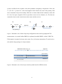
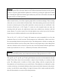
Two source-receiver systems are considered: a) vertical loops, i.e., horizontal magnetic dipole
(HMD) source and horizontal response component or b) horizontal loops, i.e., vertical
magnetic dipole (VMD) source and vertical response component. Two measurement
configurations are considered: a) in-line (along the flight line) and b) broadside (perpendicular
to the flight line). Figures 1a and 1b illustrate the coaxial and coplanar loop (HMD) AEM
systems used by the Geological Survey of Finland. Note that although AEMINV was
originally developed for airborne applications, it can also be used to interpret ground EM data
and VMD systems such as Apex Maxmin II (Fig. 1d). The EM response of the loop-loop
3
system is defined as the in-phase (real) and quadrature (imaginary) components of the ratio
Z = [Htot /H0 - 1], where Htot is the total magnetic field, which is the sum of the primary field
due to transmitter loop and secondary field due to currents induced into conductive earth, and
H0 is the free-space magnetic field at equivalent source-receiver distance (L). The data are
assumed to locate at the center between the source and the receiver.
a)
Rx
c)
b)
Pi(x,y,h)
Tx
flight line
loop spacing, L
Figure 1. Schematic view of three loop-loop configrations often used in geophysical EM
measurements: a) (coaxial) inline HMD, b) (coplanar) broadside HMD, c) inline VMD. The
EM response is assumed to locate at the center Pi(x,y,h) between transmitter (Tx) and receiver
(Rx) and the loop spacing (L) is kept constant.
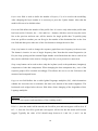
AEM data location Pi(x,y,h)
flight line
ground level
1, 0, 1=0
layer thickness, ti
2, 0, 2 (i)
overburden
basement
Figure 2. Schematic view of two-layer resistivity model used in AEM inversion.
4
1.1 Requirements and setup
AEMINV requires a PC with MS Windows (Vista/7/8) operating system and a graphics
display with a resolution of at least 1024768 pixels. Memory requirements and processor
speed and are not critical factors, since dynamic memory allocation is used and the
computations are rather fast even on older computers. AEMINV has a simple graphical user
interface (GUI) that is used to handle file input and output, to set inversion parameters and to
visualize the measured and computed EM data and the resulting pseudo-sections. The user
interface and visualization are based on the DISLIN graphics library.
The distribution file (AEMINV.ZIP) can be downloaded from author's web-site at the
University of Oulu, Finland (https://wiki.oulu.fi/x/EoU7AQ). The distribution file contains a
32 and 64-bit executables (AEIMINV.EXE & AEMINV64.EXE), dynamic link library for
OpenMP parallelizations (LIBIOMP5MD.DLL for 64-bit version only), this description file
(_README.TXT), an user's manual (AEMINV_MANU.PDF), and two example data files
(EXAMPLE.DAT and GENERIC.DAT) and example result files for 1-, 2- and 3-layer cases.
To install the program, simply unzip Pkzip/7zip) the distribution file onto hard disk and a new
folder will appear.
5
2. User interface
In the beginning AEMINV reads graph parameters from the AEMINV.DIS file. If this file
cannot be found a new one with default parameter values is created automatically. The
program then displays the standard (Windows) Open file dialog so that the user can select the
file that contains the measured EM data. The *.DAT file extension and mask is used by
default for data files that contain only single profile and a predefined header. The program
then computes the synthetic response of the initial two-layer model. Finally, the program
builds up the GUI and creates graphs of the measured and modelled data and the layered earth
resistivity model (see Appendix A). If the user cancels the open file operation the graph area
will be blank.
Note: Multiple profile lines can be read from (Geosoft) XYZ files (File/Read XYZ data) but
only after the GUI has already started up. Thus, when data is to be read from an XYZ file one
can choose to cancel the initial open file operation (e.g. pressing ESC key). See chapter 4 for
more information on file formats.
2.1 Menus
The main window of the AEMINV application has three menus. The File menu:
open and read measured data from *.DAT file
open and read measured data from *.XYZ file
save the measured and computed data into *.OUT file
read previously saved layered earth model from *.LAY file
save the current layered earth model into *.LAY file
read new graph parameters from *.DIS file
save the graph in Adobe's Postscript format
save the graph in Adobe's Encapsulated Postscript format
save the graph in Adobe's PDF format
save the graph in Windows metafile format
save the graph in GIF-compressed format.
6
Selecting any of these options brings up a typical Open/Save file selection dialog that can be
used to provide the name and directory location for the file. Data files are stored in text
format. The graphs are saved as they appear on the screen in landscape A4 size.
The AEMinv menu has following sub-menus:
choose loop-loop system (VMD and HMD)
choose loop configuration and define system parameters
enable data weights and parameter roughness and set thresholds
define distances in meters, kilometers, feet or miles
choose between five different color scales
change some other graphical setting.
Note that usually horizontal magnetic dipoles (vertical loops) are used in airborne applications
and vertical magnetic dipoles (horizontal loops) are used in ground applications (Slingram
a.k.a HCPL or HLEM). The inline HMD configuration is a coaxial loop system and the
broadside HMD system is a co-planar loop system (cf. Figure 1). Perpendicular systems
(VMD-HMD or HMD-VMD) cannot be modeled. This is because AEMINV uses a 1-D
model and interpretation of perpendicular systems would benefit from 2-D modelling. The
Configuration/Set system parameters menu item can be used to define: 1) loop spacing, 2)
frequencies and 3) nominal flight altitude.
Data weights are used to increase or decrease the importance of individual data points in the
inversion. The weights are read from the input data file together with the measured data. If
weights do not exist the corresponding menu item Weights on/off will be inactive. Likewise,
Roughness on/off item is used to activate or inactivate roughness (and to draw or hide the
roughness lines in the pseudo-section).
Set thresholds item defines thresholds for small in-phase values (MIN_RE), maximum data
spikes (MAX_SPK) and minimum singular values (MIN_SVA). The first one is used to free
fix/free status of magnetic susceptibility in the initial model. By default the magnetic
properties of all those data points whose in-phase component is higher than MIN_RE value
7
are not inverted at all (the pseudo-section will be white). When data is read in, in-phase and
quadrature values that deviate from the surrounding values more than the MAX_SPK are
rejected. If MAX_SPK= 0, all data values are accepted. MIN_SVA defines the minimum
value of the normalized singular values used as Marquardt factors in the SVD based inversion
method. The value is defined in percents indicating that, for example, the default value of
0.01 is actually 0.0001. Thus, all singular values that are smaller than 1:10000 compared to
the largest singular value will be damped. Normally there is no need to change the threshold.
Increasing MIN_SVA above the default value produces stronger damping which leads to
slower convergence. Decreasing MIN_SVA may lead to unstable inversion as the inversion
will start to resemble steepest descent algorithms.
Note: All distances (loop spacing and flight altitude, depth to the top and layer thicknesses)
used in the computations are defined in metres. Since the inversion is performed point-bypoint the actual data coordinates can be anything. Distance units menu item only adds correct
unit on the x axis below the response graph and pseudo-section. It does not redefine depths,
heights and distances in actual computations.
The Miscellaneus sub-menu:
show or hide resistivity labels in the pseudosection
show or hide black horizontal lines between layers
show or hide skin depth curve in the pseudosection
show/hide profile start and end coordinates
show/hide markings for fixed parameters
swap between normal and alternative data scaling
use alternative scaling for the data
reverse the sign of the measured data
reverse (mirror) the profile direction
swap between parts-per-million (ppm) and percentage (%)
change or edit the two title lines of the graph
8
The dynamic range of AEM data can be several decades and, hence, the low amplitude
anomalies are difficult to see clearly. Alternative data scaling makes it possible to see better
the fit between measured and computed data for small in-phase and quadrature component
values. Reversing the data sign might be useful when reading coaxial data that is normally
negative but that, for some reason, has been stored as positive values. Reversing the profile
direction not only affects the way it is shown in the graph but will also cause the new data and
layer model to be saved in reverse order. Usually AEM data are defined in parts-per-million
units whereas ground data are defined in per-cents. The Swap ppm/% item thus allows
AEMINV to normalize the computed response correctly. When alternative data scaling is
used the y axis units are displayed as (*) instead of (ppm) or (%).
The Exit menu has two items. The Restart wide/norm -item will rebuild the GUI and swaps
between traditional 3:4 aspect ratio and widescreen displays. When changing to widescreen
mode the program asks the user for a scaling value, which is less than one for widescreens,
equal to one for 3:4 screens and more than one for rotated screens.
The Exit menu has two items. Restart wide/norm item is used to close and restart the whole
GUI using a screen aspect ratio that suites either old 3:4 displays or widescreen displays.
When changing from normal to widescreen mode the program asks for an aspect ratio value
(0.7-0.8 is good for most widescreens). Ok to Exit item is used to confirm the exit operation.
On exit the graph parameters, current results (measured and computed data) and the model are
automatically saved into AEMINV.DIS, AEMINV.OUT and AEMINV.LAY files,
respectively. Errors that are encountered before the GUI starts up are reported in the
AEMINV.ERR file. Inside GUI mode run-time errors are displayed on the screen.
2.2 Controls
Update button is used to validate the changes made to text fields, to perform forward
computation, and to refresh the graph accordingly. Note that pressing Update is not always
necessary, but usually it does not hurt to press it either. When starting optimization, for
example, the values of global and local Lagrange multipliers are automatically checked.
9
Layers text field is used to define the number of layers (1-3) to be used in the modelling.
After changing the layer number it is necessary to press the Update button. After that the
model will reset to its default values.
Line text field defines the number of the profile line. It is active only when multi-profile data
has been read in. Likewise, the <-Line and Line-> buttons, which are used to swap the active
line to the previous and next one, will be inactive for single profile data. To quickly jump
from one profile to another you can first give the number of the destination line on the Line
text field and then press either one of the Line buttons to change the active line.
Swap freq button is used to change the response graph from one frequency to the next one.
The button is inactive in case of single frequency data. Note that the actual frequencies (in
Hz), the loop spacing and the nominal flight altitude are defined when the data is read in, but
they can be redefined via the Aeminv/Configuration/Set system parameters menu item.
Swap comp button can be used to show only the in-phase (real) or the quadrature (imaginary)
component or both data components. When changing the data component the y axis of the
response graph will be rescaled accordingly. This allows the user to see the fit between the
measured and computed better.
Lagr.sca text field defines the so-called global Lagrange multiplier (LG), which determines
whether the inversion tries to minimize the data error instead of the model roughness. The
horizontal scale widget below the text field allows faster changing of the (logarithm of the)
Lagrange multiplier.
Important: The global Lagrange multiplier is the most important inversion parameter, which
affects the convergence and smoothness of the resulting model.
If LG > 1, then the model will be smooth, the fit will be poor and convergence will be slow. If
LG < 1, then the fit will be good and convergence will be fast but the model will become
rugged. Typically the value of LG should range between 0.1 and 10 (-1 and 1 on the
10
logarithmic scale widget). Note that both the data and the model parameters are scaled using
the maximum data variation and maximum parameter variation (resistivity scale limits and
depth limits). Therefore, the default value (LG = 1.0) provides rather good compromise
between data fit and model smoothness, but the convergence may be rather slow. Therefore,
the Lagrange multiplier should be decreased in the beginning of the inversion and increased
after sufficient fit has been obtained to obtain smoother model.
Im-scale defines a relative weight (WI) between in-phase and quadrature components. By
default (WI= 1.0) the two components have equal importance in the inversion. Decreasing WI
gives quadrature component less importance in the inversion. Vice versa, increasing WI
reduces the importance of the in-phase component. This parameter should be used if the other
response component is much noisier and lower in amplitude than the other.
F-length defines the filter length (FL) used to compute the parameter roughness (default FL =
2). The roughness is defined as the difference of the parameter pi from the mean of the
surrounding points pi*= [(ij.pj), j= i-FL,i+FL]/(2FL), where ij is Kronecker's delta function.
The longer the filter is, the smoother is the resulting Occam model and the less sensitive the
model is to data noise.
Iters # defines the number of successive iterations to be performed when the Optimize button
is pressed (default 10 iterations).
Z-wght defines a local Lagrange multiplier (LZ) for the parameter corresponding the depth to
the top of the model. Note that LZ should be equal to zero in two- and three-layer inversion, in
which the topography of the top layer should be fixed to zero level. In half-space inversion,
however, it should be non-zero (by default LZ= 0.01). Decreasing LZ below 0.01 makes the
topography more rugged and increasing LZ above 0.01 makes the topography smoother.
Optimize button performs a given number of inverse iterations. The inversion is based on
linearized inversion scheme. The sensitivity matrix is constructed numerically using forward
differences. The linear system is solved for the parameter steps using singular value
decomposition (SVD) together with adaptive and automatic damping.
11
The two radio buttons below the Optimize button are used to decide whether the inversion is
performed only for the current profile or all profiles one at a time (Current line vs All lines).
Alternatively, if only one profile has been read in, the inversion is made only for the zoomed
part or the whole profile length (Zoomed part vs Full length).
The six text fields below the optimize button are used to define the default or initial values
(left column) and local Lagrange multipliers of the model parameters (resistivities R1, R2, and
R3 and thicknesses T1 and T2). Depending on the number of layers the extraneous text fields
will be invisible. The local Lagrange multipliers are used to control the lateral variations of
each individual parameter. Increasing the value (Li >1.0) makes lateral variations smoother
and decreasing the value (Li < 1.0) allows larger lateral variations. Typically Li-values should
range between 0.1 and 10.
Important: Setting the Li value equal to zero will exclude that parameter from the inversion,
which is essentially the same as if the parameter is fixed for all data points.
Default button is used to reset all model parameters to those in the text fields above.
The four text fields below Default button allow the user to redefine the minimum and
maximum resistivity values and the minimum and maximum depth in the pseudo-section. The
limiting resisitivity values shown on the color scale (10-base logarithms) and the depth to the
bottom of the pseudo-section are also used as the limiting parameter values in the inversion.
In other words, the inversion cannot make the resistivity of a layer smaller than the minimum
resistivity value shown on the color scale and the thickness of a layer greater than the
maximum depth. Note that initially the minimum depth is defined by the flight altitude.
Zoom/Pan button allows zooming in to a section of a profile. When applying the button the
program goes into editing mode and the normal arrow cursor becomes a crosshair cursor
above the graph area. The user makes selections pressing the left and right mouse buttons as
discussed below.
12
Important: Zooming and all other mouse editing functions work in a similar fashion. To zoom
in the user presses the left mouse button at two different horizontal locations on the pseudosection or response graph and then updates the selection by pressing the right mouse button
once. Pressing the right mouse button again without any selections will end the edit mode and
program returns to normal operation.
When zoomed in the y axis of the response graph will be rescaled accordingly. Thus zooming
allows the user to see the details of the data better. Note that zooming can be used to limit the
inversion so that the parts of the profile outside the current zoom area are unaffected in the
inversion (Zoomed part vs Full length). To zoom out to the original extent one enters the
zooming mode and presses the right mouse button once (without any selections with left
mouse button). To pan the zoomed view left and right the user needs to press the left mouse
button only once and then update the screen with right mouse button.
The fix R1, fix T1, fix R2, fix T2 and fix R3 buttons are used to manually fix (or free) the
parameters from (or to) the inversion. Fixed parameters are indicated by a white cross above
the corresponding element in the pseudo-section. The editing mode is similar to zooming: the
the left mouse button is used to select points. However, the program stays in the editing mode
and more elements can be selected or previous ones can be unselected until the right mouse
button is pressed twice in a row (i.e., without any left mouse clicks in between).
Important: If a single left mouse click is made outside the profile (left to the beginning or
right to the end of the profile), then all the block elements of that parameter are set free.
The rgh R1, rgh T1, rgh R2, rgh T2 and rgh R3 buttons are used to set discontinuities into the
model. These allow (but do not necessitate) a jump in layer boundary or resistivity at that
point. The editing mode is similar to fix/free status editing, with the exception that the
discontinuities are located between two model blocks. Discontinuities are indicated by white
vertical (resistivity) or horizontal (thickness) lines between the block elements in the pseudosection. As with fix/free status editing, if a single left mouse click is made outside the profile,
then all discontinuities are removed from that parameter.
13
The res R1, res T1, res R2, res T2 and res R3 buttons are used to reset the corresponding
parameter to its (arithmetic) mean. If discontinuities have been set in the model, the mean is
computed between them (see Appendix D). This option helps the user to create rough
(categorical) interpretation model.
The edit R1, edit T1, edit R2, edit T2 and edit R3 buttons are used to manually edit the
position of layer boundaries and resistivity values. When thicknesses are edited the vertical
position of the mouse click defines where the layer boundary should be positioned. Likewise,
when resistivities are edited the current color scale appears at the end of the pseudo-section
and the vertical position of the left mouse click defines what resistivity value should be given
to that point. Single left and right mouse button clicks are used to change model values pointby-point. If two points are selected (two left mouse clicks are made), then linear interpolation
is made between those points. If multiple points are selected with left mouse, then spline
interpolation is applied through those points. If a single left mouse click is made outside the
profile (eg. above the color scale), then layer boundary or resistivity is reset to the
corresponding value along the whole profile and the selected value is updated in the default
text field.
3. Interpretation procedure
When the data are read in, also the measurement system (VMD vs. HMD), loop configuration
(in-line vs. broadside), loop spacing and frequency (or frequencies) are set. The loop spacing
should be checked and corrected if needed. To validate changes made to the text fields one
needs to press the Update button.
Initially the number of layers is 2, which allows separation of conductive overburden and
basement. When single layer model is used the Z-wght parameter should be non-zero to allow
the inversion of the depth to the top of the conductive half-space. When multi-frequency data
are available, the user may want to try to interpret the thickness of conductive targets. This,
however, may be ambiguous, because real targets are often two-dimensional and AEMINV
uses layered earth model. The skin depth curve should be used to assess if the EM system is
capable of "seeing through" conductive layers.
14
Important: A previously computed and stored layer model can be opened after data has been
read in. Before, reading the *.LAY file, it is necessary that the number of layers is set
according to that used in the data. Since the initial number of layers is two, the user must
change it to one before reading a one-layer model.
The user should then pay attention to the default values of the layer parameters. The initial
resistivity and thickness values depend on the problem (frequencies, loop spacing and true
earth conductivity) and the user should experiment with their values to allow the inversion to
start from a good initial guess. Normally, the initial resistivity model should be a
homogeneous half-space unless there is some a priori information against this assumption (eg.
more conductive overburden). After editing the text fields of the default values the user can
press the Default button (without pressing Update button) to reset the initial model.
The inversion can now be started by pressing the Optimize button. Usually the convergence is
rather slow when the default value of global Lagrange multiplier is used and the optimization
must be made multiple times before good fit is achieved. Therefore, user may want to
decrease the Lagrange multiplier at the beginning and increase it later to create smoother
model. To see if stable solution is found the user should pay attention to the data RMS and
model RMS in the upper right corner of the graph as well as to any visible changes in the
pseudo-sections. To see finer details in the fit one can swap between different response
components using Swap comp button, try using the Alternative scaling menu-item and/or
zoom into a section of the profile using Zooming button.
Without any discontinuities the constrained inversion will create a quite smooth model. After
few basic inversions one should have a pretty good idea where there might be lateral
conductivity or thickness variations. Using the editing buttons for model roughness (rgh R1,
rgh T1, etc) one can define discontinuities. After this few more optimization runs should be
made to see how the model changes. Alternatively, after editing discontinuities one might
disturb the model using the resetting buttons and start the inversion from a new initial model.
15
If the user has any a priori information, for example about the thickness of the overburden at
some point, then one can use the editing buttons to set the thickness or resistivity at some
point and then the fixing buttons to fix that value during inversion. The constrained inversion
will then (try to) adjust the neighboring elements to fit the fixed value to minimize the model
roughness. Alternatively, one can save the current model into a *.LAY file and manually edit
the parameter values and fix/free values.
The user should always test different models and different values of the various inversion
parameters (particularly the global Lagrange multiplier and the separate parameter weights).
As often in geophysical interpretations there is no unique inverse model. The practice,
however, will create masters.
Because of dynamic memory allocation, the only limit for the total number of data points is
the available computer memory. However, since single profile is considered, simultaneous
processing of large datasets should be avoided because the graph will get too crowded. In
principle, however, it is possible to process multiple lines by putting discontinuities between
the lines and invert the whole dataset blindly and use external software to create maps of layer
conductivity and thickness.
16
4. File formats
4.1 Formatted data files
Before starting up the program make sure that your input files are formatted properly.
Currently EM data can be read in three formats: a) preformatted DAT files, b) generic column
formatted DAT files and c) Geosoft XYZ files, which support multiple profiles.
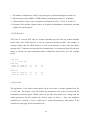
The format of the preformatted input data file is shown below.
Line 591
1 25. 1 0
1 2 5
3220 3 4 0
! nof, loop, HMD, coaxial
! x, y, z
! fre, re, im, wgh
35496.00 70981.00
35497.00 70980.00
35498.00 70980.00
...
-49
-48
-20
-40
-6
23
32
30
30
The 1.st line defines a header text (max. 80 characters), which is used as a secondary title
above the response graph. The 2.nd and 6.th line are used for comments and can be left
empty. Usually the header line should define the name of the measurement site and possibly
the number of the profile line. If the header line is empty the default title in the AEMINV.DIS
file will be used instead. Note that the Edit title lines menu item can be used to redefine the
titles and if the secondary title (initially set in the *.DIS file) is not blank it will take
precedence from that of the data file. To disable the fixed secondary title and to enable the
title line of the data file one should give blank line for the secondary title using Edit title lines
menu item.
The 3.rd line defines the 1) number of frequencies (NOF), 2) loop spacing (L, in meters), 3)
loop orientation (VMD= 0, HMD= 1) and 4) loop configuration (inline= 0, broadside= 1).
Note that loop spacing and measurement system can also be defined inside the GUI so it is
not required to remember their codes.
17
The 4.th line defines the column indices (ICOX, ICOY and ICOH) of the x and y coordinates
and the flight altitude (meters). If altitude data is not available the corresponding column
index should be zero (ICOH=0). In this case the elevation of all data points is set equal to the
value given in Height text field in GUI control panel. Note that the x axis of the graphs is the
profile distance computed from the beginning of the profile (e.g., di= [(xi-x0)2+(yi-y0)2]1/2). If
any of the column indices (ICOX, ICOY, ICOH) is negative the profile direction will be
reversed (actual coordinates are preserved). If x or y coordinates are missing (or only profile
distance is available) the corresponding column index should be set equal to zero (ICOX= 0
or ICOY= 0). Note that the profile distance (x axis) must be in an ascending order also when
x or y coordinates are missing. The profile will be reversed automatically if the profile
distance computed as di= (xi-x0) or di= (yi-y0) would become decreasing.
The 5.th line defines the frequency (F1, in Hertzes) of the first dataset and the column indices
of the in-phase (ICI1) and quadrature (ICQ1) components and data weights (ICW1). Data
weights are used to increase (wgh > 1) or decrease (wgh < 1) the importance of individual
data points. If the data file does not include data weights, the corresponding column index
should be set to zero (ICW=0). If the file contains data from two or more frequencies, the
frequencies (F2) and column indices (ICI2, ICQ2, ICW2) of the successive datasets would be
defined on the next (NOF-1) lines. The remaining NOP lines define the actual data in column
format. Lines starting with "#", "/", or "!" characters are considered to be comment lines.
4.2 Generic data files
If the input data file starts with a "#", "/", or "!" character it is considered to be in a generic
column format and the user needs to provide all the necessary header information
interactively. Any other lines that start with these characters are considered comment lines
and they will be ignored. The example below illustrates the format of the generic data file.
# Generic data file
# x y re im h
35516.00 70982.00
35516.00 70983.00
...
-27
-9
-16
-1
27
30
After opening a generic data file the program asks for:
18
1. The number of frequencies (NOF), loop spacing (m), and nominal flight elevation (m).
2. Measurement system (HMD vs VMD) and loop configuration (inline vs. broadside),
3. Column indices of the x and y coordinates and altitude (ICOX=1, ICOY=2, ICOH=5),
4. Frequency (Hz) and the column indices of in-phase and quadrature components and data
weights for each frequency.
4.2 XYZ data files
XYZ files or Geosoft XYZ files are column formatted text files that can contain multiple
profile lines. The LINE directive is used to separate individual profiles. The number or
character string after the LINE directive is used as an identifier or title of the line. Rows
starting with "/" character are interpreted as comment lines. As with generic data files the user
needs to provide the abovementioned header information interactively. See the example
below:
/XYZ file
/ X Y H
LINE 100
35516.00
35516.00
...
LINE 101
35616.00
35616.00
...
RE
IM
70982.00
70983.00
27
30
-27
-9
-16
-1
70981.00
70983.00
29
31
-37
-11
-26
-10
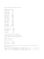
4.3 Layer files
The parameters of the layered earth model can be saved into a column formatted text file
(*.LAY) and The header of the file defines the parameters used in the inversion and the
normalized root-mean-square (RMS) values of the data and model error. Along with the
model parameters the file includes the fix/free status (0=fixed, 1= free), the roughness
parameters (0= smooth, 1= left, 2= right and 3= totally discontinuous). Note that to fit the
example on single page it has been edited a bit.
19
# Results from AEMINV: the interpreted 2-layer model
#
# Computational parameters:
# Lagrange scale
1.0000
# Im-scale (im/re)
1.000
# Filter length
2
# Re/Im hide value
10.000
# Z_elev weight
0.00000
# Rho 1 default
10000.0
# Rho 1 weight
1.000
# Thick 1 default
50.000
# Thick 1 weight
1.000
# Rho 1 default
5000.0
# Rho 2 weight
1.000
# Rho minimum
0.1000
# Rho maximum
100000.0
# Thick minimum
-63.000
# Thick maximum
200.000
#
# Susc minimum (SI)
0.000010
# Susc maximum (SI)
10.00
# Susc default
0.001
# Susc weight
1.000
#
# Thickness in meters, resistivity in Ohm-meters
# Listed conductance values (S) are multiplied by 1000
# Listed susceptibility values (SI) multiplied by 1000
#
# Number of layers: NL=
2
# Number of lines: NOLIN=
1
#
# Data RMS error:
0.270092E-01
# Model RMS error:
0.207693E-01
#
# X, Y, Dist, Skin, Z, Rho1, Thi1, Rho2, Sus2, Cnd1, fxZ, fxR1, fxT1, fxR2, rgZ, rgR1, rgT1, rgR2, fxS, rgS
# Number of points: NP=
118
1654 8299
0.00 366.63 0.0000 100000.0000 227.1138 292.9494 1.0000 2.2711 1 1 1 1 0 0 0 0 0
1691 8303 37.22 471.85 0.0000 100000.0000 313.9914 401.6601 1.0000 3.1399 1 1 1 1 0 0 0 0 0
1728 8306 74.34 407.13 0.0000 92188.8281 234.1963 456.0468 1.0025 2.5404 1 1 1 1 0 0 0 0 1
0
0
0
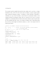
4.4 Output files
The measured and the modelled data and the data weights can be saved into a column
formatted text file (*.OUT). The file can be used, for example, to prepare response graphs
using commercial third-party software. In addition to useful descriptive information a
commented (#) copy of the file header is stored before the actual data columns. If the
comment characters preceding the header lines are removed, the file can be read into
AEMINV as a preformatted data file. Otherwise the format conforms to that of a generic data
file. The computed data (Re_c & Im_c) are located in columns 6 and 7 and measured data
(Re_m & Im_m) and weights are located in columns 8, 9, and 10. An example of the file
format is given below.
#
#
#
#
#
#
#
#
#
#
#
#
#
#
#
Results from AEMINV: computed and measured EM data
1 25.000
1
2
4
3220.00 8
1
0
9
10
! #freqs, loop spacing, HMD/VMD, inline/broadside
! x, y & altitude column
! freq, re, im & weight column
Number of lines:
1
Total number of data:
236
Number of frequencies:
1
Frequencies (Hz): F = 3220.0
Loop spacing (m): L =
25.00
HMD source
Inline configuration
Units = parts-per-million (ppm)
# Line
1
# x, y, d, h(m), z(m), Re_c, Im_c, Re_m, Im_m, wgh
# 118
! number of points
35516. 70982.
0.000 27.00 0.00 -20.34 -17.56 -27.00 -16.00
35516. 70983. 37.216 30.00 0.00
-9.56
-9.06 -9.00 -1.00
35517. 70983. 74.337 32.00 0.00 -14.74 -14.96 18.00 -17.00
...
1.00
1.00
1.00
4.5 Graph options
Several graph parameters (see Appendix A) can be changed editing the AEMINV.DIS file.
This allows translating the graph texts into other languages, for example. Note that the format
of the AEMINV.DIS file must be preserved. If the format becomes invalid or if you replace
the AEMINV.EXE file with different version, you should delete the graph parameter file and
a new one with default parameter values will be generated automatically the next time the
program is started. The file format and default values are shown below.
# Aeminv
1.30 parameter file
32
32
24
16
1
1
1
1
1
1
2
1
300 300 0.85 0.67 0.70
0.10000 100000.00
-63.00
200.00
10.00
5000.00
10000.00
50.00
5000.00
50.00
10000.00
0.001000
0.00000
1.000
1.000
1.000
1.000
1.000
1.000
1
1
3
0
4
1 2 3
25.00
30.00
0
3220.000
AEM interpretation
1-Layer model
2-Layer model
3-Layer model
Distance
Real
Imag
Real m
Real c
Imag m
Imag c
Resistivity ({M2}W{M1}m)
Depth (m)
Height
Skin
Susceptibility (SI)
 The 1.st line is a comment line defining the file version
 The 2.nd line should be left empty.
 The 3.rd line defines four character heights. The first one is used for the main title and the
graph axis title, the second is used for the axis labels, the third is used for the plot legend,
and the fourth is used for the resistivity labels of the pseudo-section.
22
 The 4.th line defines The remaining parameters define: 1) flags for normal vs. widescreen
display, 2) show/hide resistivity labels, 3) show/hide line between layers, 4) show/hide
skin depth curve, 5) show/hide fix/free status, 6) flag for ppm (parts-per-million) or %
(percentage) response, 7) index number of color scale., and 8) flag for symbols or
solid/dotted line for measured in-phase and quadrature data.
 The 5.th line defines first the 1) x (horizontal) and 2) y (vertical) position of the origin of
the main graph (in pixels) from the bottom-left corner of the page and then the length of
the 3) x and 4) y axes relative to the size of the total width and height of the page (eg. 0.5 =
50 % of the width or height), which is equal to 29702100 pixels (landscape A4), 5) the
aspect ratio for widescreen display. Aspect ratio is equal to 1 for 3:4 and about 0.8 for most
widescreen displays. Note that in vertical direction the length defines the relative height of
both the response plot and the pseudo-section since both graphs are equally high.
 The 6.th line defines the 1) minimum (R_min) and 2) maximum (R_max) value of the
logarithmic EM response axis (ppm or %), 3) minimum (Z_min) and 4) maximum
(Z_max) values of the depth axis (m), 5) the threshold for small in-phase values, and 6)
maximum spike value. Note that the depth axis is positive downwards and that the
minimum depth is usually based on the maximum value of the recorded airplane height.
 The 7.th line defines the default values for 1,3) resistivity (m) and 2,4) thickness (m) of
the first and second layer and 4) the resistivity and 5) magnetic susceptibility of the
basement.
 The 8.th line defines the default weights for 1,3) resistivity (m) and 2,4) thickness (m) of
the first and second layer and 4) the resistivity and 5) magnetic susceptibility of the
basement.
 The 9.th line defines first 1) the measurement system (0= VMD, 1= HMD) and 2)
configuration (0= in-line, 1= broadside) and then the column indices of the 3,4) x and y
coordinates and 5) airplane elevation.
 The 10.th line defines 1) the number frequencies (NOF) and 2) loop spacing and 3)
nominal flight altitude.
 The next NOF lines define the column indices of the 1) in-phase (real) and 2) quadrature
(imaginary) data components, 3) weight and 4) frequency. Please, note that the parameters
on lines 9-10+NOF are used to store the previous values when reading XYZ files and
generic data files that do not contain file header.
23
 The next line should be left empty.
 The following lines define various text items of the graph (max. 80 characters).
o Main title line of the response graph.
o Second title line of the graph (used if the data file does not include a title).
o Three possible title lines of the layered earth model graph (currently not used at all).
o Title of the x axis (defined in the data file - usually the distance along profile).
o Two y axis names for the response graph.
o Four legend names of the response graph (measured and computed data).
o The label of the color scale defining resistivity. Note that the "log10" label is added in
front of the color scale label automatically.
o The vertical axis name of the resistivity pseudo-section (always meters).
o The legend names for the auxiliary flight height and skin depth curves.
o The label of the color scale defining susceptibilty.
Special characters "{" and "}" should not be used in any text strings, because they define
instruction strings that enable Greek symbols. Other instruction characters that must be
avoided are: "^" for superscripts, "~" for subscripts and "_" for setting the baseline back to its
original position. Please, see DISLIN manual for more information about the topic.
24
5. Additional information
The numerical computation of the EM (loop-loop) response of the layered earth is based on
the solution in Keller and Frischknecht (1967) and Frischknecht et al. (1991). The (quasistatic) solution does not take into account the effect of permittivity i.e. dielectric constant
( = 0). Non-zero magnetic susceptibility (k = r-1) is assigned only for the basement layer;
all other layers are non-magnetic ( = 0). The Hankel transforms are computed by a
convolution algorithm based on that of Anderson (1984). The optimized filter coefficients
have been computed using Christensen’s (1990) algorithm. The parameter optimization is
based on a linearized inversion method, where singular value decomposition (SVD) with
adaptive damping is used. The inversion method has been described in my PhD thesis
(Pirttijärvi, 2003). The lateral constraining is adapted from the GRABLOX program I have
made for 3-D block model inversion of gravity data. See GRABLOX2 user guide (Pirttijärvi,
2009) for more information about the Occam inversion method.
AEMINV was written in Fortran90 and compiled with Intel Visual Fortran XE 14. The
graphical user interface is based on the DISLIN graphics library (version 10.3) by Helmut
Michels (http://www.dislin.de). Since DISLIN graphics library is available for other operating
systems (Solaris, Linux, Mac) AEMINV could be compiled and run on these platforms
without any major modifications. However, I do not intend to provide active support for the
program and the source code will not be made available. If you find the computed results
erroneous or have suggestions for improvements, please, inform me.
5.1 References
Anderson, W.L., 1984: Fast Hankel transforms using related and lagged convolutions. ACM
Trans. on Math. Software, 8, 344-368.
Christensen, N.B., 1990. Optimized fast Hankel transform filters. Geoph. Prospecting 38,
545-568
Frischknecht, F.C., Labson, V.F., Spies, B.R. and Anderson, W.L. 1991: Profiling methods
using small sources. In: Nabighian, M.N. (ed.) Electromagnetic methods in applied
geophysics, Volume 2, Applications. SEG, p. 105-270.
25
Keller, G.V., Frischknecht, F.C., 1966: Electrical methods in geophysical prospecting.
Pergamon Press.
Pirttijärvi M., 2003. Numerical modeling and inversion of geophysical electromagnetic
measurements using a thin plate model. PhD thesis, Acta Univ. Oul. A403, Univ. of Oulu.
Pirttijärvi, M. & Lerssi, J., 2006. Laterally constrained 1D inversion of airborne
electromagnetic data. Abstract B020, Technical programme Near Surface 2006, Helsinki.
Pirttijärvi M., 2009. Gravity interpretation and modeling software based on 3-D block models,
User's guide to version 2.0. University of Oulu, Department of Physics,
<https://wiki.oulu.fi/download/attachments/20678029/Grablox2_manu.pdf>
5.2 Terms of use and disclaimer
You may use the AEMINV program free of charge. If you find the program useful, please,
send me a postcard. If you publish results computed with AEMINV, please, provide a notice
"AEMINV © University of Oulu" (without the quotes). When referring to the program,
please, use either the conference paper (Pirttijärvi. & Lerssi, 2006) or this user manual, e.g.,
"Pirttijärvi, M., 2014. AEMINV; Laterally constrained 1-D inversion of EM data, Version 1.3
user's guide. University of Oulu, Department of Physics < https://wiki.oulu.fi/x/PIU7AQ>".
The program is provided as is. The author (M.P.) and the University of Oulu disclaim all
warranties, either expressed or implied, with regard to this software. In no event shall the
author or the University of Oulu be liable for any indirect or consequential damages or any
damages whatsoever resulting from loss of use, data or profits, arising out of or in connection
with the use or performance of this software. All in all, use AEMINV at your own risk.
26
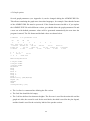
Appendix A: AEMINV GUI at startup
Program controls at the left, graph area at the right with response on top and model cross-section at the bottom. The measured data are
plotted with symbols and computed response with (solid and dotted) lines. The dotted line on top of the cross-section depicts flight altitude
variations. The vertical white lines depict automatically defined discontinuities in the basement layer.
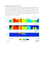
Appendix B: AEMINV GUI after inversion
The inversion result was obtained after 20 iterations (2 runs) using the default inversion parameters shown in the left control panel. The
black line on the cross-section depicts cumulative skin depth. RMS-d and RMS-m are the data and model RMS values.
28
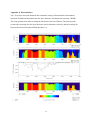
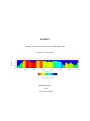
Appendix C: Three alternative inversions
Top: The half-space resistivity and depth to the top (flight height) were optimized, whish is
similar to the traditional apparent resistivity transformation. Middle: The depth to the top was
fixed and the parameters of the two-layer earth were optimized. This gives the same result as
the first inversion if the resistivity of the top layer is very high. Bottom: The resistivity of the
top and bottom were fixed to 10000 m and the depth, thickness and resistivity of the
conductive middle layer were optimized.
Appendix D: 2-frequency AEM data
Combined inversion of two-frequency (3.124 & 14.363 kHz) AEM data (coplanar HMD’s)
using a two-layer model. Note the presence of conductive overburden at the beginning of the
profile (Imag>Real). The separation between the overburden and basement conductors could
be improved by setting discontinuities at selected points.
30
Appendix E: Discontinuities
Top: Two-layer inversion obtained after automatic setting of discontinuities and manual
insertion of additional discontinuities for layer thickness and basement resistivity. Middle:
The same psudosection after resetting the basement resistivity. Bottom: The same pseudosection after resetting also the layer thickness and overburden resistivity and the resulting fit
between the measured and modelled data above it.
31