Download IMP Software Suite User Manual

IMP Software Suite User Manual
Release 1.2
Intermodulation Products AB
May 26, 2015
CONTENTS
1
Introduction
1.1 Conventions and useful tips . . . . . . . . . . . . . . . . . . . . . . . . . . . . . . . . . . . . .
1.2 Screen Layout . . . . . . . . . . . . . . . . . . . . . . . . . . . . . . . . . . . . . . . . . . . .
1.3 Python . . . . . . . . . . . . . . . . . . . . . . . . . . . . . . . . . . . . . . . . . . . . . . . .
3
3
3
3
2
The IMP Session and Work Flow
2.1 Quick Start . . . . . . . . . . . . . . . . . . . . . . . . . . . . . . . . . . . . . . . . . . . . . .
2.2 The Work Flow . . . . . . . . . . . . . . . . . . . . . . . . . . . . . . . . . . . . . . . . . . . .
5
5
5
3
Quantitative Analysis
3.1 Inspecting single pixels . . . . . . . . . . . . . . . . . . . . . . . . . . . . . . . . . . . . . . .
3.2 Analyzing lines and surfaces . . . . . . . . . . . . . . . . . . . . . . . . . . . . . . . . . . . . .
19
19
23
4
Advanced Topics
4.1 Intermodulation Measurement . . . .
4.2 Noise Calibration . . . . . . . . . . .
4.3 Programming your own Force Models
4.4 Data Tree . . . . . . . . . . . . . . .
4.5 Advanced Setup . . . . . . . . . . .
4.6 Drive Constructor . . . . . . . . . .
4.7 Stream Recorder . . . . . . . . . . .
4.8 Scripting Interface . . . . . . . . . .
4.9 Scan Data . . . . . . . . . . . . . . .
4.10 File Management . . . . . . . . . . .
4.11 Panels and Views . . . . . . . . . . .
.
.
.
.
.
.
.
.
.
.
.
.
.
.
.
.
.
.
.
.
.
.
.
.
.
.
.
.
.
.
.
.
.
.
.
.
.
.
.
.
.
.
.
.
.
.
.
.
.
.
.
.
.
.
.
.
.
.
.
.
.
.
.
.
.
.
.
.
.
.
.
.
.
.
.
.
.
.
.
.
.
.
.
.
.
.
.
.
.
.
.
.
.
.
.
.
.
.
.
.
.
.
.
.
.
.
.
.
.
.
.
.
.
.
.
.
.
.
.
.
.
.
.
.
.
.
.
.
.
.
.
.
.
.
.
.
.
.
.
.
.
.
.
.
.
.
.
.
.
.
.
.
.
.
.
.
.
.
.
.
.
.
.
.
.
.
.
.
.
.
.
.
.
.
.
.
.
.
.
.
.
.
.
.
.
.
.
.
.
.
.
.
.
.
.
.
.
.
.
.
.
.
.
.
.
.
.
.
.
.
.
.
.
.
.
.
.
.
.
.
.
.
.
.
.
.
.
.
.
.
.
.
.
.
.
.
.
.
.
.
.
.
.
.
.
.
.
.
.
.
.
.
.
.
.
.
.
.
.
.
.
.
.
.
.
.
.
.
.
.
.
.
.
.
.
.
.
.
.
.
.
.
.
.
.
.
.
.
.
.
.
.
.
.
.
.
.
.
.
.
.
.
.
.
.
.
.
.
.
.
.
.
.
.
.
.
.
.
.
.
.
.
.
.
.
.
.
.
.
.
.
.
.
.
.
.
.
.
.
.
.
.
.
.
.
.
.
.
.
.
.
.
25
25
26
29
29
31
33
36
38
39
44
46
Installation
5.1 Install Software .
5.2 Install Hardware
5.3 Set AFM Type .
5.4 Common AFMs
.
.
.
.
.
.
.
.
.
.
.
.
.
.
.
.
.
.
.
.
.
.
.
.
.
.
.
.
.
.
.
.
.
.
.
.
.
.
.
.
.
.
.
.
.
.
.
.
.
.
.
.
.
.
.
.
.
.
.
.
.
.
.
.
.
.
.
.
.
.
.
.
.
.
.
.
.
.
.
.
.
.
.
.
.
.
.
.
.
.
.
.
.
.
.
.
.
.
.
.
.
.
.
.
.
.
.
.
.
.
.
.
.
.
.
.
.
.
.
.
.
.
.
.
.
.
.
.
47
47
47
48
49
The Multifrequency Lockin Amplifier MLA™
6.1 Capabilities . . . . . . . . . . . . . . . . .
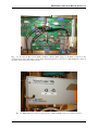
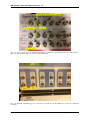
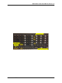
6.2 Connections . . . . . . . . . . . . . . . .
6.3 Firmware . . . . . . . . . . . . . . . . . .
6.4 MLA version I (before 2015) . . . . . . .
.
.
.
.
.
.
.
.
.
.
.
.
.
.
.
.
.
.
.
.
.
.
.
.
.
.
.
.
.
.
.
.
.
.
.
.
.
.
.
.
.
.
.
.
.
.
.
.
.
.
.
.
.
.
.
.
.
.
.
.
.
.
.
.
.
.
.
.
.
.
.
.
.
.
.
.
.
.
.
.
.
.
.
.
.
.
.
.
.
.
.
.
.
.
.
.
.
.
.
.
.
.
.
.
.
.
.
.
.
.
.
.
.
.
.
.
57
57
57
58
59
5
6
.
.
.
.
.
.
.
.
.
.
.
.
.
.
.
.
.
.
.
.
.
.
.
.
.
.
.
.
.
.
.
.
.
.
.
.
.
.
.
.
.
.
.
.
7
Trouble Shooting
61
8
References
63
Bibliography
65
i
ii
IMP Software Suite User Manual, Release 1.2
Contents:
CONTENTS
1
IMP Software Suite User Manual, Release 1.2
2
CONTENTS
CHAPTER
ONE
INTRODUCTION
The Intermodulation Products Software Suite (IMP Suite) from Intermodulation Products AB is a collection
of software tools for performing Intermodulation Atomic Force Microscopy (ImAFM™) – a powerful surface
analysis method based on multifrequency AFM. This manual explains how to use the IMP Suite through its
Graphical User Interface (GUI). The manual is used most effectively when the IMP Suite is open and running,
taking data with your host AFM or analyzing already scanned data.
1.1 Conventions and useful tips
The IMP help icon appears at several places in the IMP Suite. Clicking on this icon will open a browser and
jump to the appropriate place in the manual.
Screen text is denoted with a shaded box and it should coincide exactly with text in the IMP Suite; on a
button, or next to a check box or input field.
The genindex contains key words and important screen text. Each entry is linked to the appropriate place in the
manual. If you are wondering about the function of a button in the software use the help icon or search for the
button name in the genindex.
Linked text (e.g. The IMP Session and Work Flow) cross-references to different parts of the manual. Use the back
button on your browser or PDF viewer to return to the jump point.
Bullet lists are used to describe related items which appear in a group. For example, groups of radio buttons,
control settings or groups of output fields, all related to a particular task.
1.2 Screen Layout
The screen layout in the software can be customized to suit the users needs, and the actual appearance depends on
the computer platform used (Linux, Windows, Mac). A detailed discussion of how to customize the screen layout
is given in the advanced section on Panels and Views. For this reason we do not make extensive use of pictures or
screen shots in the manual, but rather screen text and icons
.
1.3 Python
The IMP Software Suite is written in the computer language called Python, an open source language with many
powerful tools for plotting, image analysis, and numerical calculation. These are collected in a set of modules
called SciPy (Scientific Python)). The IMP Suite is platform-independent, running on Windows, Macintosh or
Linux. Native graphics environments are used in the GUI which is written in wx-Python , so icons and panels may
appear slightly different on different platforms.
This manual is written in restructured text language, and is available as HTML or PDF. The HTML version is
linked with the help icons in the IMP Suite and it is more easily used when working with the Suite online. A
separate software developer documentation describes the usage and function of the Python objects which make up
3
IMP Software Suite User Manual, Release 1.2
the IMP Suite. The developmer documentation is designed for users who want to enhance the functionality of the
software by modifying the source code and programming their own measurement and analysis methods.
4
Chapter 1. Introduction
CHAPTER
TWO
THE IMP SESSION AND WORK FLOW
2.1 Quick Start
Connect the intermodulation lockin to your host AFM and make sure the switch(s) on your signal access module
are in the correct position. For details on connecting to your AFM, please consult the Install Hardware section.
Start the host AFM and set it to Contact Mode, with the feedback set-point set to zero volts. Here we assume
that zero volts on the detector corresponds to the equilibrium position of the cantilever when it is free from the
surface.
Start IMP Software Suite. A session folder named with the current date is automatically created where all your
data will be stored.
2.2 The Work Flow
The work flow is symbolically represented by the left column of 6 Im icons. From top to bottom, these icons guide
the work flow in the IMP Suite. Click on these icons to open the different panels and views.
Find the resonance by performing a Frequency Sweep.
Calibrate the cantilever using non-invasive thermal noise Calibration.
Set up and start a scan then engage the surface with the host AFM to start Scanning.
Open previous scan files and use the pixel and line inspectors to Analyze Scan Data.
5
IMP Software Suite User Manual, Release 1.2
Add comments to the automatic logging in the Session Logbook.
View the session and import host AFM data, batch process, or view 3D parameters maps in Session Overview.
Each step in the work flow is described in detail in the following sections:
2.2.1 Frequency Sweep
After loading the cantilever and adjusting the detector, we find the cantilever resonance by sweeping the frequency
of the cantilever drive signal while measuring the detector response signal. The Frequency Sweep panel opens
when you click the top icon in the work-flow.
Run sweep starts the measurement between the Start frequency and Stop frequency. Edit these
fields to change the sweep range. The sweep range should include the likely resonance frequency of the cantilever,
which should be provided by the probe manufacturer and is usually printed on the probe box. Reducing the
measurement Bandwidth causes the sweep to be slower and the measured response to be more accurate. The
sweep speed also depends on the Number of points recorded during the sweep.
Two check boxes provide automatic features for finding the resonance:
• Locate peak performs a second sweep with finer detail, zoomed in on the peak response found in the
sweep range.
• Transfer results to noise calibration transfers the center frequency and estimated sweep
range to the next stage in the work flow.
Correcting Driven Response
Use Correction is an advanced function that can be left unchecked for simple resonance-finding. This
function is used to ‘de-embedd’ linear response from the measurement chain. Sometimes electronic equipment
between the output or input of the Multifrequency Lockin Amplifier™ (MLA™), (see Intermodulation Measurement) and the host AFM can cause frequency-dependent amplitude and phase shifts to the signals that are
measured by the MLA™. Use Correction compensates for any undesirable linear transfer of the signal due to
these compenents ‘embedded’ in the measurement chain. The compensation is made using a procedure called
de-embedding, performed in two steps:
1. A frequency sweep is performed while by-passing the AFM (insert a short in place of the AFM). After
this sweep, press the Set Correction button, which transfers the result of this sweep to an internal
correction file.
2. Put the AFM back in to the measurement chain and check the Use Correction check-box. All subsequent sweeps performed with this box checked will correct for the amplitude and phase shifts measured in
the first step.
In summary:
6
Chapter 2. The IMP Session and Work Flow
IMP Software Suite User Manual, Release 1.2
• Use Correction will correct the measurement for an arbitrary linear, frequency-dependant transfer
function embedded between the output and the input points of the measurement chain.
• Set Correction stores the last-measured transfer function to an internal file which is used for the
correction.
2.2.2 Calibration
Quantitative AFM starts with a good calibration of the cantilever and ImAFM™ requires this calibration before
you start to scan a surface. The IMP Software Suite contains the latest methods for cantilever calibration based
on the measurement of the thermal Brownian motion of the cantilever and a theory of hydrodynamic damping of
the oscillating beam. By fitting a theoretical model to the noise data we determine all constants necessary to the
measure the cantilever deflection in meters, and convert this deflection to force in Newtons.
The calibration procedure applies to a particular cantilever eigenmode (resonance). Details and references to the
literature are given in the advanced section on Noise Calibration. Here we describe how to perform the calibration.
The tab at the very top selects between calibration of a Flexural or Torsional eigenmode. The procedure is
very much the same for either type of mode, but the underlying formulas and analysis are different. We begin by
describing calibration of flexural eigenmodes, and end with a discussion of torsional eigenmodes.
Choose Cantilever and Method
Calibration Parameters specifies the type of cantilever and calibration method.
• Temp [C] is the temperature of the damping medium in Celsius, used to determine the magnitude of the
thermal noise fluctuation force driving the cantilever.
• Fluid selects the density and viscosity of the medium surrounding the beam, needed for calculation of
hydrodynamic damping. Noise calibration methods have not been tested thoroughly beyond studies in Air,
but we include to option to apply the theory in Water 20 C.
• Cantilever selects from a list of pre-programed cantilevers for which calibration constants have been
published. If your cantilever is not on this list you can choose Arbitrary Rectangular and enter the
Length and Width , or plan-view dimensions of your rectangular beam cantilever. You can edit the length
and width fields for any chosen cantilever without changing the stored values for pre-programed cantilevers.
Alternatively, you can Add Edit Remove cantilevers as described below.
• Method selects between six methods of calibration:
– Hydrodynamic function uses an analytic expression for the hydrodynamic function to calculate
the damping. The calculation applies to a rectangular beam in the limit length >> width (see [Sader1998]). This method uses length and width given in the fields above.
– Sader constants uses a good approximation to the hydrodynamic function described with three
parameters 𝑎0 , 𝑎1 , 𝑎2 that are specific to a particular cantilever. These constants have been measured
and checked against other methods and according to theory they should apply to any cantilever of the
same shape (see [Sader-2012]). For this method, the length and width fields have no influence.
– Reference calibration brings up three fields. If you have one good calibration using another
means, such that you know all three constants: the quality factor, stiffness and resonant frequency, or
Q-ref, k-ref and f0-ref respectively, you can use this calibration as a reference for calibrating
other cantilevers of the same shape (see [Sader-2012]). For this method, the length and width fields
have no influence.
2.2. The Work Flow
7
IMP Software Suite User Manual, Release 1.2
– Thermal tune: responsivity brings up a field to enter the known stiffness of the cantilever
fundamental eigen mode, k [N/m]. The thermal noise measurement is then applied to determine the
detectors inverse responsivity [nm/V].
– Thermal tune: stiffness brings up a field to enter the known detector inverse responsivity,
Inv. resp. [nm/V]. The therm noise measurement is then applied to determine the cantilever
mode stiffness.
– Manual overrides the thermal noise measurement and no hydrodynamic damping theory is applied.
All four calibration constants are entered in the fields given: the eigenmodes resonance frequency
f0 [Hz], dimensionless quality factor Q [-], mode stiffness k [N/m], and the detectors inverse
responsivity Inv. resp.[nm/V].
Measure noise
Acquire Data controls the start of measurement, saves data, or loads previous measurement data.
• Run calibration starts the averaging of many separate noise measurements, to decrease the fluctuations in the noise data. If Frequency Sweep was used to find the resonance and Transfer results to
noise calibration was activated, the software will automatically analyze an appropriate frequency
range around the resonance. The Status Banner indicates the progress of the calibration.
• Settings opens an Acquisition Settings dialog box where you can select the total number of
Measurements in the average, the Center frequency [kHz] and Frequency span [kHz]
to analyze, and the Frequency resolution [Hz] between data points. You can also give a
Down-sampling factor which averages the given number of samples before transferring to the computer
for spectral analysis.
• Save As opens a dialog box to save the noise data to a .txt file. If Autosave is checked, this file
will be automatically saved. The file is saved in the JSON format, and it can easily be opened in many
different programing languages (Matlab, Python, Java, etc.) It is not necessary to save the raw noise data
for each calibration, as the software automatically keeps track of the Current calibration, or most recent fit
of calibration data, which is stored as the relevant calibration in the scan file.
• Load opens a dialog box to load a previously saved noise data.
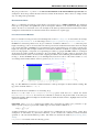
Fitting noise data
When the Enable Fit box is checked, the fit is performed in real time and displayed in the plot as a solid blue
line. The noise contribution from the cantilever motion is shown with the yellow dash line. For a full description
of the theory and fit, see Noise Calibration.
Sometimes very low level spurious signals can be picked up when measuring noise. If the spurious signal is not
driving the cantilever, you can remove improve the calibration by removing them from the fit. Select the following
tools in the calibration plot toolbar:
•
•
•
•
right-click-and-drag on the plot will select a range where the fit will be performed. Data outside this
range becomes grey and is not analyzed in the fit.
clears the selected fit range.
right-click-and-drag defines an area over which data points are ignored in the fit. The removed data is
marked with a red x.
clears all ignored data.
Calibration Result
The Calibration Result is displayed in several ways giving you important figures of merit. It is useful
to think of the calibration as having two parts: The calibration of the cantilever (the force transducer) and the
8
Chapter 2. The IMP Session and Work Flow
IMP Software Suite User Manual, Release 1.2
calibration of the detector (the deflection sensor, or optical lever).
Cantilever:
√︀
• Resonance frequency 𝑓0 = 𝑘/𝑚[kHz] of the simple harmonic oscillator model used to model the
cantilever eigenmode with mode stiffness 𝑘 and effective mass 𝑚.
• Width of resonance 𝛾[Hz] related to the damping coefficient of the simple harmonic oscillator
model. 1/𝛾 is the characteristic time for exponential decay of oscillation amplitude due to the damping
of the surrounding medium.
• Quality factor 𝑄 = 2𝜋𝑓0 /𝛾 is the ratio of the energy stored in the oscillation, to the energy lost per
cycle of oscillation. A freely oscillating cantilever will ‘ring’ for 𝑄 cycles before the amplitude decays by a
factor of 1/𝑒, or 37%.
• Cantilever stiffness 𝑘[N/m] is the eigenmode stiffness, or the coefficient of the linear restoring
force in the simple harmonic oscillator model.
√
• Thermal noise force [fN/ Hz] is the fluctuation force associated with the linear, viscous damping
of the cantilever. This frequency-independent force noise gives rise to a peak in the deflection noise near a
high-Q resonance. The thermal noise force represents a fundamental sensitivity limit for force measurement
(see Note on sensitivity and accuracy).
Detector:
• Inverse responsivity |𝛼|−1 [𝜇𝑚/V] is the inverse magnitude of the detectors response function,
which converts the measured signal in Volts [V] to a deflection of the tip in meters [m]. In the literature,
this constant is often referred to as the ‘inverse optical lever sensitivity’ (invOLS), but we prefer the term ‘
responsivity’ (see Note on sensitivity and accuracy for further discussion) . The calibration performed here
actually does not rely on a calibrated measurement of voltage by the MLA™, nor does it rely on the calibration of the AFM scanner to determine detector responsivity. The software uses the noise measurement
to determine cantilever deflection in the digital counting units of the MLA™, or Ananog-to-Digital units
[ADU]. Thus, the noise measurement and hydrodynamic theory together become a primary form of calibration that does not depend on the calibration of any other equipment, apart from the thermometer measuring
temperature.
√
• Noise floor [fm/ Hz] is the detector noise, expressed as an equivalent deflection noise of the cantilever.
This figure is the correct measure of the sensitivity of the opto-electronic system which detects the cantilever
deflection.
√
• Equivalent force [fN/ Hz] expresses the detector noise as and equivalent force noise acting on the
cantilever. This equivalent force noise gives the sensitivity of force measurement, if the same cantilever
were to measure force quasi-statically, or at low frequency well below resonance.
• Peak to flat ratio [dB] is the ratio of the noise peak (thermal noise) to the flat background noise
(detector noise). If you compare two measurements with the same cantilever, the larger this number, the
better your detection (see Note on sensitivity and accuracy).
Current calibration
Running a new calibration, loading a previous calibration, selecting a new range or excluding points, runs the
fitting routine which determines all the calibration constants. These constants define the current calibration.
After each scan, all calibration constants from the current calibration are stored with the scan file, together with
the raw spectral data acquired by the MLA™. It is not necessary to store a calibration file in order to analyze the
data in scan file. The Store and Load features are there only if you want to store or view raw noise data for a
particular run of the calibration. The raw noise data will be saved for each run if Autosave is checked. It is very
easy to re-calibrate during a scan session and thereby re-define the current calibration. Simply stop the scan, retract
the probe from the surface, and re-run the calibration. We recommend that you re-calibrate frequently, to check if
anything has changed with the cantilever and detector. Calibration should also be re-run if any adjustments have
been made to the laser or the detector, and it must be performed with every new cantilever, before you start to
perform ImAFM™.
2.2. The Work Flow
9
IMP Software Suite User Manual, Release 1.2
Add Edit Remove cantilevers
Add / Edit / Remove opens a dialog box that allows you to change calibration parameters of one of the
stored cantilevers, or to create a new cantilever.
The Add tab has two options:
• Basic is for rectangular cantilevers. Enter the Length, L [um] and Width, b [um] in micrometers, and the cantilever name and manufacturer. Click Add and your cantilever will appear in the pull-down
list. The calibration method will will be based on the theoretical expression for the hydrodynamic damping
function, valid for 𝐿 >> 𝑏 (see Method above).
• Advanced is for cantilevers of arbitrary plan-view dimensions. Here you can enter the Sader
Constants if they are known, or the calibration parameters of a Reference calibration for a
cantilever of the same plan view dimensions (see Method above). Length and Width are interpreted as
effective values for a non-rectangular cantilever.
The Edit tab allows you to change calibration parameters of the selected cantilever.
The Remove tab allows you to remove a user-added cantilever from the selection list.
Calibrating torsional eigenmodes
Torsional calibration uses the same principal flexural calibration. It is currently under development and two
methods are available:
• Hydrodynamic Function uses the analytical expression for the hydrodynamic function of a long rectangular beam, calculated by Green and Sader [Green-????]. This method calibrates the fundamental eigenmode and it uses length and width given in the fields above.
• Thermal tune: stiffness brings up a field to enter the the height of the tip, or the distance that
the tip is offset from the principle axis of the cantilever beam ???.
2.2.3 Scanning
Before you begin, the host AFM must be configured for ImAFM™. If no special ImAFM™ mode is provided on
your host AFM, simply put it in contact mode with the feedback set-point set to zero volts. The MLA™ generates a ‘fake’ deflection signal and the host AFM will preform scanning feedback on this signal (see Connection to
host AFM). The feedback parameters, integral and proportional gain, are set in the host AFM software.
The default scanner view has three components: The Scanner panel, the Image Settings panel and the
main view showing the Amplitude and Phase images. More panels can be added, for example when you want
to perform analysis as you scan, making force curves or analyzing transects. These panels will be addressed in the
section on Quantitative Analysis. Here we describe how to setup and execute the first scan.
Setup and Scan
Three controls in the Scanner panel specify the parameters for Setup. There must be a Current calibration in
order for the setup to function.
• Osc. range is the desired maximum amplitude of oscillation (peak-to-peak) in nanometers of the cantilever when it is free from the surface. When the surface is engaged, the oscillation range will be somewhat
reduced, depending on the Amplitude set point.
10
Chapter 2. The IMP Session and Work Flow
IMP Software Suite User Manual, Release 1.2
• Mod. range is the range over which you want to modulate the amplitude. The amplitude will be modulated from the minimum value ( Osc. range - Mod. range ) to a maximum value Osc. range.
The tip-surface forces will be measured over this range. Typically you want to measure from zero deflection,
up to the peak value of the cantilever deflection. In this case you set the modulation range to one half of the
oscillation range.
• Pixel rate (df) is the spacing ∆𝑓 between tones in the frequency comb (see Intermodulation Measurement). The pixel rate, together with the number of pixels per line determine the scan rate.
• Resolution: x y sets the number of pixels to acquire in the fast scan direction (x) and the slow scan
direction (y). The x resolution does not depend on the host AFM setting of pixels per scan line. The x
resolution together with the pixel rate determines the Scan Rate given by the IMP Suite. The scan rate
must be set on the host AFM to the value given by the IMP Suite. The y resolution must also be set to the
same value on the host AFM, which determines the number of scan lines at the given rate.
• Setup runs a routine to determine the frequency and amplitude of the two drive tones. If you get an
Out of Range Error message you may need to adjust the oscillation range or attenuate the input signal
(see Advanced Setup). This automatic setup is designed for basic ImAFM™ with two drive tones close to
resonance. Much more complicated measurements and modulation schemes can be setup with the Drive
Constructor. When the setup is complete, the Scan button will not have gray text, indicating that you are
ready to scan.
Scan makes the software ready to acquire measurement data. After pressing Scan:
• Set the scan rate on the host AFM to the Scan rate given in the scanner panel.
• Make sure your host AFM is set to contact mode and the set-point is set to zero volts.
• Engage the sample and start the scan in the host AFM software.
When the end-of-line (EOL) triggers are detected, the IMP Suite will begin to collect and display the scan data.
After the last scan line when an end-of-frame (EOF) trigger is detected, a scan file is stored (see Status Banner).
However, the EOL and EOF triggers do not code for the direction of the scan. It may be necessary to sometimes
Flip left-right or Flip up-down to make your image match that displayed on the host AFM.
On some AFM’s you can move to the top or bottom of a frame to start a fresh scan without waiting for the current
scan to finish. If this action is performed on the host AFM, and if the EOF trigger is sent, the IMP will save
a scan file and automatically start collecting a new scan. Some AFM’s (notably Asylum) do not send and EOF
trigger when you move to the top or bottom of a frame. When the IMP suite is configured for such an AFM, two
buttons appear which allow you to Move to top or Move to bottom to keep the synchronization with the
host AFM scan.
During the scan, you can at any time perform the following actions and set the following parameters:
Measure free, set-point, scan rate
Measure free causes the cantilever to be pulled away from the surface where a new measurement of the free
response is made. The tip-surface force is determined by subtracting the free response from the engaged response.
The free response is automatically measured durring Setup, but not between continuously acquired scans. The
most recent measurement of the free response is stored with the scan file when it is saved at the end of the scan,
and this most recent measurement is used for subsequent analysis. Often the cantilever needs to ‘settle in’ after
engaging a surface, and a new measurement of the free response is required after some time of scanning. We
recomend that you press Measure free if your force curves appear strange, to check and see if this makes a
difference.
Amplitude set-point is the set-point for the AFM feedback. Feedback is based on the response amplitude
at one of the two drive frequencies (Drive 1), and the set-point is given as a percent of the free response amplitude
at this drive frequency (see Setup Feedback). To engage the surface, this set-point must be below 100%. Setting
the set-point to more than 100% will cause the probe to lift from the surface – a useful way to lift away from the
surface without stopping the scan, if you want to check or adjust something.
Scan rate is the required rate of scanning as determined from the pixel rate and x resolution. The scan rate is
determined by the chosen pixel rate (measurement bandwidth, df) and number of pixels in the scan line (x resolu-
2.2. The Work Flow
11
IMP Software Suite User Manual, Release 1.2
tion). You must set the host AFM to scan at the given scan rate, otherwise the images will not be synchronized.
Some host AFMs do not allow arbitrary scan rate and it is not necessary that the scan rates match exactly. A
1% deviation is not noticeable in the images, but one should set the host AFM scan rate slightly smaller than the
ImAFM™ scan rate. You can slow down the scan rate using the same measurement bandwidth and pixel rate, to
help track better on a rough surface. normal means scanning at the maximum rate and you can choose half or
quarter speed. Making this choice will result in a new calculation of the scan rate which must be set in the host
AFM. Slowing down the scan will help to track the surface more closely, making the force measurement more
accurate.
You can also change to new values of Osc. range and Mod. Range during a scan. Input the new values ad
press Setup. The cantilever will lift and perform a new setup routine, adjusting to the new parameters. However,
you can not change the value of Pixel rate (df) without first stopping the scan and lifting away from the
surface.
Image settings
The panel Image Settings contains the controls for displaying which images are plotted
• IMP Control lets you select the frequency at which the Amplitude and Phase images are plotted.
The frequencies are ordered from lowest to highest, going from left to right. The text below the slider
displays which frequency is being plotted
• Scan direction has two buttons which control whether the Trace or Retrace will be plotted. Data
is acquired and stored for both scan directions. Note that both trace and retrace are always stored in every
scan. Flipping between trace and retrace can be a good way to see if feedback errors are affecting your
image.
• Swap will exchange the data stored as trace and retrace. The host AFM trigger signals do not distinguish
between different scan directions, and sometimes it is necessary to swap so that trace and retrace are the
same as that in the host AFM. Do not worry if you do not get this correct during the scan as it can be easily
corrected after the scan session using the Session Overview.
• Flip right-left and Flip up-down do not exchange trace and retrace data. This action can also
be done later in the Session Overview.
• Scan size , when checked, will display axis labels with the image size which must be entered in the x
and y data fields. Units should be given in either nanometers or micrometers, using the characters: nm, um
or µm (u will be displayed as µ). Scan size values will be stored when the scan is saved, and these values
will be overwritten if and when the scan size is imported together with height data from the host AFM (see
Import host AFM data).
Color Bar
The color bars have functionality for adjusting the images:
• Right click on the color bar to see a histogram of the plotted values. You can adjust the image contrast by
left-click-and-drag on the borders to the shaded region. These borders mark the max. and min. values for
12
Chapter 2. The IMP Session and Work Flow
IMP Software Suite User Manual, Release 1.2
the color map used. Data outside the shaded region is forced to either min. or max. If the check box is
activated, the software will automatically choose the max. and min. excluding the given percent of outlying
values. You can also change the color map in the histogram window.
• Click-and-drag upward or downward on the color bar, to adjust the minimum and maximum values respectively. The color value of the center will remain constant. You can do this action with the histogram
open.
• Double click on the color bar to return to the automatic setting settings.
Image Toolbar
All plots and images have a toolbar with the following functions:
Home, Forward and Back tools
The home tool to returns to the initial plot or the full image. The forward and back buttons move through the
successive plot views which the software remembers after each zoom or pan action.
Pan-Zoom
When selected, left-click-and-drag will cause the plot to zoom, starting from the point of click. Dragging horizontally will zoom only the x-axis, dragging vertically will zoom only the y-axis. Dragging at an angle controls
the relative rate of zoom of each axis. Right-click-and-drag will grab the plot at the point of click and slide it in
the direction of the drag. Performing these actions while holding down the x, y or ctrl keys will restrict the pan or
zoom to occur only in the x-axis, y-axis, or preserving current aspect ratio, respectively.
Zoom
When selected, a right-click-and-drag over the plot will zoom to the selected rectangle upon release.
Save image
Opens a dialog box for saving the image in several formats (png, eps, pdf and more). Sometimes you would like
to change the aspect ratio of the plot, or the relative size of the frame and text in your saved image. Simply rescale
the entire suite (click-and-drag on the lower right corner), or re-size a particular frame, before you save. This
action will rescale the plot and axes while keeping the text and line size fixed.
Configure subplots
The subplots icon opens up a dialog box to adjust the placement of the plot axes within the plot frame.
Selecting Data in a Scan
Two important tools in the image toolbar are the pixel inspector and line inspector tools. These tools do more than
simply controlling the plot. They select data at pixels and analyze the data to generate force and parameter plots.
Pixel inspector tool
A left-click on the icon will activate this tool. When the tool is activated, a right click on either the amplitude or
phase image will select the data at the point-of-click, mark it with an X, and open the Signal Inspector panel. If
you have the Quantitative Analysis tools installed in your software, the Force Inspector will also open and display
a force curve. When the pixel inspector tool is active, left-click on the plot will un-select the X nearest to the
point-of-click and remove the data from the Data Tree. The Quantitative Analysis tools allow you to analyze
the spectral data in many different ways to reveal tip-surface interaction. The Data Tree allows you to compare
different pixels form the same scan, or different scans, in the same plot.
2.2. The Work Flow
13
IMP Software Suite User Manual, Release 1.2
Line inspector tool
A left-click on the icon will activate the tool. When active, a right-click-and-drag on either the amplitude or phase
image will select a transect line upon release and a left click will un-select the line nearest to the point-of-click.
The Line Inspector panel will open and a plot of the amplitude and phase of the currently viewed image will
be shown. All data along this line will be selected and available for analysis. If you have the Quantitative Analysis
tools installed in your software, the line inspector will allow Analyzing Linear Transects and plot parameters of
the tip-surface interaction along the selected transect.
Status Banner
The banner at the very bottom of every view has text describing what task the software is currently performing
(sweeping, calibrating, scanning, etc.) and a status bar that graphically shows the time required to finish the task.
If Autosave is checked data is continuously saved to file save when the task is finished. The name of the most
recent saved file is also given.
2.2.4 Analyze Scan Data
One aspect of ImAFM™ which makes it so powerful is that all raw data, trace and retrace, are stored in one
compact scan file. The intermodulation spectrum at each pixel is an optimally compressed representation of the
cantilever motion, from which we reconstruct the tip-surface force. With the raw data stored in the scan file, the
AFM scientist can go back and make a more careful study of each point on the surface, analyzing it with different
models and plotting it in different ways. To fully appreciate the analytical power of Intermodulation AFM, you
should have the Quantitative Analysis package from Intermodulation Prodcuts.
In File pull-down menu, select Open (ctrl+O). The Amplitude and Phase images appear in a new tab
for each open scan file. You can open multiple tabs and compare data from different scans on the same plot in the
analysis view. In the analysis view you will find the Image settings panel, the Image Toolbar and the Color Bar
which have functions previously described. With the Pixel inspector tool and Line inspector tool, you can select
individual pixels and lines for Quantitative Analysis.
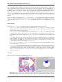
Image Smoothing
The analysis panel has an additional Smooth image button, which opens a smoothing dialog box where you can
apply a Gaussian filter to your scan data. This filter will convolve the stored intermodulation data with a Gaussian
function of width in x and y given by Sigma, in pixels. The result is a new image, stored to the given File
name, where each pixel of the new image is a weighted average of neighboring pixels in the raw scan data file.
Smoothing with one pixel results little loss of sharpness in the image but it lowers then noise considerably. The
Gaussian has 98% of the weight within 3 Sigma of the center, so smoothing with one pixel essentially averages
a block of 9 pixels, giving an improvement in the signal-to-noise ration by a factor of 3. This is a smart way to
improve the signal quality without increasing the measurement time, based on the assumption that neighboring
pixels are more likely to have the same response. Note however that smoothing does introduce a correlation length
14
Chapter 2. The IMP Session and Work Flow
IMP Software Suite User Manual, Release 1.2
to your data, which you can clearly see as a grainularity in high-order IMP images, which are often more noisy.
Be careful not to interpret these smoothing-induced grains as features in your image.
2.2.5 Session Logbook
The Intermodulation AFM Software Suite keeps a session log while you are working. This log file is a text file
formatted for easy reading so you can quickly see exactly what was measured and when it was measured. The
software automatically logs all important activity in chronological order with a time stamp. For example: making
a new calibration, storing an image, starting or stopping the scan, and much more.
You can also add your own text comments to the log file. Add your comment to text field at the bottom of the
panel and finish with Ctrl+Return. Your comment will be time stamped in inserted in to the log file.
2.2.6 Session Overview
This view shows all the scans in a session, automatically imports data from the host AFM, sorts out unwanted
scans to a sub-folder, adjust images for synchronization problems with the host AFM, and generates parameter
maps on multiple scans in a batch processing mode.
Session
Open IMP session and choose a session folder. An overview is generated showing file info and image thumbnails where each row corresponds to one scan. Reload causes the overview to be updated to the current state of
the session folder. View session log opens a window showing the session log file.
Import host AFM data
The AFM height image is a record of the change of the probe height during the x-y scan. The probe height ℎ,
is the position of the base or the fixed end, not the position of the tip 𝑧 at the free end, of the flexing cantilever
(see drawing in the section Force Reconstruction Methods). The probe height is controlled by the feedback while
scanning, and in most modern AFMs the height signal is measured using a linear sensor built in to the scanner.
When performing ImAFM™, the height data is recorded by the host AFM. To associate ImAFM™ quantitative
analysis with surface topography, it is necessary to import the height data in to the IMP Software suite.
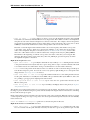
Associate host AFM files
• Import height data : Navigate to the folder on your host AFM computer, network or storage device
where the host AFM files are stored. When you OK the selected folder the Match Images window
opens. Drag the image thumbnails from Unmatched IMP images at the bottom, and drop them on
the corresponding AFM images at the top. When you have matched a few images, click Match with
timestamps and the computer will attempt to associate all remaining files. If the matching is incorrect,
you can drag images away from middle group of Matched IMP images. When the matching looks
correct, click OK and a copy of the AFM height data files will be stored in the ImAFM™ session folder with
the scan number (i.e. scan01234_) prefixing the host AFM file name. The AFM height data will remain
in the same file format as the Host AFM. (Note: In DI/Veeco Nanoscope software version 5 there is a bug
2.2. The Work Flow
15
IMP Software Suite User Manual, Release 1.2
which requires you to simply open and close the file in the DI software before you can import it to the IMP
suite.)
• Hide unchecked will move all the unchecked scans to a sub-folder of the session folder called ‘hidden_scans’. These scans will no longer be displayed in the session overview, but they are not erased. You
can always use your computers file browser to move a file from the ‘hidden_scans’ folder back to the session
folder, where it will again be displayed when you click Reload. Unhide all brings all files from the
‘hidden_scans’ sub-folder up to the session folder.
Flip and swap scans
Because the host AFM does not code the trigger signals for trace and retrace (only for change of fast-scan direction) it may be necessary to left/right flip the scan data or exchange the trace and re-trace data in order to associate
the ImAFM™ scan correctly with the host AFM scan. Furthermore, AFM triggers do not code for slow scan
direction (only end of frame) so it may be required to exchange up/down flip images. All this is easily done in the
Session Overview. To perform these these flip and swap operations you first have to select the scans.
Checkmarks control which files will be flipped and swapped: Check will select all scans, Uncheck deselects
all scans, Toggle will switch checked to unchecked, and unchecked to checked.
Apply to checked scans
• Flip Left/Right is performed on both trace and retrace data, but trace and re-trace are not exchanged.
• Flip Up/Down is performed on both trace and retrace data, but trace and re-trace are not exchanged.
• Swap Trace/Retrace will exchange trace and retrace, with out performing any flip. Note that left-right
flip, does not necessarily imply that trace and retrace were stored incorrectly when scanning. Depending
on whether you selected the trace or retrace for storing the height data in the host AFM, you may want to
exchange trace an retrace to get correct association. ImAFM™ always stores both trace and retrace.
Batch process parameter maps and force volume data
Analyze checked scans in the Session Overview lets you set up and run a batch process to make parameter
maps on several files.
• Paramter Map: Model fit, when checked, will perform the analysis described in Model Fit, generating parameter maps, or color coded images of tip-surface force parameters. The settings button
opens a panel for choosing the model and fit parameters, as described in Parameter Maps.
• Paramter Map: Polynomial, when checked, will perform the anaysis described in Fast Polynomial, based on the polynomial representation of the conservative force-distance curve. The settings
button opens a dialog with options similar to that for Parameter Maps. Polynomail degree is desribed
in Polynomial.
• ADFS Force Volume , when checked, will perform Amplitude Dependent Force Spectroscopy (ADFS)
on each pixel of an image. The settings button opens a dialog with options similar to that for Parameter
Maps. Save to HDF5 will create one file containing an ADFS force curve at each pixel, whereas Save
to ASCII will create a folder with one file for each pixel, where the pixel coordinates are given in the file
name.
• Start the batch processing for all checked scans. A status bar tells you how far the batch process has
progressed. Abort will end the process, storing the data analyzed thus far. It is not possible to resume an
aborted process.
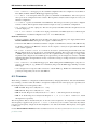
Three dimensional viewer
To generate a three dimensional view you must have imported the height data from your host AFM. Double click
on the height image to open the IMP 3D-viewer.
If you have generated a parameter map for the scan in question, the 3D viewer will paint a color map of a parameter
on to a 3D projection of the height data. In the Viewer settings group, the check box Same color-bar
16
Chapter 2. The IMP Session and Work Flow
IMP Software Suite User Manual, Release 1.2
will force the 3D viewer to use the same limits for all parameter images of the same type. This feature makes it
much easier to compare parameter maps between different scans.
When the viewer is open, you will see functionality for:
Save image as... where you can save to a desired location, and choose between several different file
formats.
Image settings
• Choose the Size of the image in pixels. Resizing the viewer to changes these numbers and their aspect
ratio.
• Background color can be chosen to something other than the default gray.
• Text color will effect the X and Y size labels.
Sample settings
• Z scale sets the aspect ratio of the Z scale, in relation to the X and Y scales. This aspect ratio is displayed
below the image, together with the Peak height in nanometers, or the height of the tallest feature in the
image.
• Parameter is pull down menu listing all parameters of the model which was fit to the scan data. Here you
select the parameter which you want to display as a color map, on the 3D view of the height data. Note that
parameters which where were unchecked in the fit settings, were not adjusted and will therefore show only
one color corresponding to their fixed value.
• Limits opens up a window with a histogram of the parameter values. The shaded region is that covered
by the color bar. Everything outside this region is displayed as white. You can click and drag on the left
and right edges of this region to adjust the color bar limits, or input the Min: and Max: values manually.
The check box at the top allows you to activate an automatic routine to adjust the limits, excluding the given
percent of pixels in the upper and lower tails of the histogram.
Camera position
• Azimuth and Polar angles can be entered as degrees, or left click and drag on the 3D image.
• Distance is changed by adjusting the control, or right click and vertical drag on the 3D image.
Plane fit has three different methods for flattening the image:
• None shows the height data as it is stored in the host AFM height image file.
• Average fits a plane over the entire image and offsets all height data so that this plane is flat.
• Selected points allows you to flatten on a selected region of the image. With this option selected,
hover over the image with the mouse. When you press the ‘p’ key, the point at the mouse arrow will be
selected. After selecting 3 points a plane can be calculated and the image will offset all height data so that
this plane is flat. You can continue to select more than 3 points, and the image will be flattened with a
best-fit plane to all selected points. The clear button removes all selected points. A red frame appears
when you select points. To make this frame disappear, hover outside the image and press the ‘p’ key.
2.2. The Work Flow
17
IMP Software Suite User Manual, Release 1.2
18
Chapter 2. The IMP Session and Work Flow
CHAPTER
THREE
QUANTITATIVE ANALYSIS
The quantitative analysis tools allow you to analyze the measured intermodulation spectral data at each pixel in
a variety of ways. Each spectrum is a frequency-domain representation of the tip motion at that pixel, and from
this motion we determine the tip-surface force. We may refer to this analysis as inversion because it involves
solving an inverse problem, or that of finding the force which produced the measured motion, as opposed to
forward problem of finding the motion resulting from a given force. As is often the case, the inverse problem is
‘ill-posed’. The limited sensitivity of our measurement gives inadequate information for finding a unique solution
to the inverse problem. The very small force that we are trying to determine only gives measurable motion at
frequencies in a narrow band close to the high-Q cantilever resonance. Our challenge is therefore to reconstruct
the force from this partial spectrum, or narrow band response. Fortunately, with enough intermodulation spectral
data, and with a few assumptions that are not so very restrictive, we can find useful solutions. We call the solution
of this inverse problem force reconstruction , or reconstructing the force from the intermodulation spectrum.
In dynamic AFM there are several forces giving rise to the cantilever motion: The tip-surface force, cantilever
bending forces, viscous drag force on the cantilever body, and the inertial forces due to acceleration of the cantilever mass, including the drive force resulting from the shaking of the cantilever base. To properly separate out
the tip-surface force from all other contributions we require two things: A good calibration of the cantilever (see
Calibration), and a good measurement of the cantilevers free motion when it is far away from the surface (see
Measure free, set-point, scan rate).
Calibration is performed at the outset of ImAFM™ and the free motion is measured before scanning. It is easy to
re-do either of these at any time during the session. We recommend that you check the calibration and perform a
new measurement of free oscillation occasionally, to see if the results are consistent with previous measurements.
The most recent calibration data and free motion spectrum are stored with each scan, at the end of the scan. These
measurements are an important part of the analysis of the scan data.
The focuses in this chapter is on how to use the software to perform different methods of analysis. References
are given to the scientific literature where the fundamental physics and mathematics of the force reconstruction
methods explained are explained in detail.
3.1 Inspecting single pixels
The intermodulation spectra at individual pixels can be analyzed by selecting the data with the Pixel inspector
tool. This puts the data in to a Data Tree and it allows you to examine it in the following panels:
3.1.1 Signal Inspector
Activate the Pixel inspector tool in the Image Toolbar, and left-click on a point in either the Amplitude or
Phase image to select a pixel (right-click to de-select). The data from this pixel is moved to the Data Tree and
the Signal Inspector panel opens where you can see the tip motion durring the selected pixel time. You
can display the motion in the following ways:
• Time signal shows a very dense plot of fast oscillations with a slowly varying amplitude envelope. Zoom
is required to see the individual oscillation cycles.
19
IMP Software Suite User Manual, Release 1.2
• Spectrum shows only the amplitude of the individual intermodulation frequency components, ploted on a
log scale. The component which is plotted with a thicker line corresponds to the amplitude and phase image
displayed. You can click on different componets in the plot, and the amplitude and the images will change
to the amplitude and phase of that frequency component.
• Phasor shows a plot where both amplitude and phase are plotted in a polar plot, or as vectors in a complex
plane.
3.1.2 Force Inspector
If the Quantitative Analysis software is installed, selecting a pixel with the Pixel inspector tool will open the
Force Inspector panel where you see plots of the analyzed spectral data, giving information about the
interaction forces at each pixel. Note that the physical units in the plots are given in calibrated nano-Newtons [nN]
and atto Joules [aJ = nN nm] vs. nanometers [nm], as determined in the Calibration step.
The Force Inspector panel has three tabs FI FQ Work Force which select the different plots as described in
detail below. The Settings button opens a panel where you find three corresponding tabs to control the different
plots.
• Force Inspector Settings panel, FI FQ and Work tabs:
– display options are chosen through a pull-down menu that allows you to select different regions
of the curve for plotting. Typically you want to choose multi-valued curves which shows
𝐹𝐼 (𝐴) and 𝐹𝑄 (𝐴) for both increasing and decreasing oscillation amplitude in the beat-cycle of one
pixel.
– Use shading check box will activate a shading of the 𝐹𝐼 (𝐴) and 𝐹𝑄 (𝐴) curves, such that the
lightest shade corresponds to the start of the pixel, and the darker shade the end. In the Signal Inspector
select the Time tab to see the beat-cycle for the selected pixel.
• Force Inspector Settings panel, Force tab contains several options were are explained in detail
in Force Reconstruction Methods.
In-phase and quadrature forces
The FI FQ tab brings up a double plot of two integral quantities, plotted versus the oscillation amplitude (not
static cantilever deflection). The plot 𝐹𝐼 (𝐴) is the force which is in-phase with the sinusoidal cantilever motion,
integrated over a single oscillation cycle of the cantilever motion. Similarly, the quadrature force 𝐹𝑄 (𝐴) is the
force which is 90 degree phase-shifted from the harmonic motion (in phase with the velocity). It is important to
note that 𝐹𝐼 (𝐴) and 𝐹𝑄 (𝐴) are not traditional AFM ‘force curves’ . They should not be compared to plots of
the instantaneous force vs. distance between the tip and surface, or plots of measured cantilever deflection vs.
the quasi-static probe height. Every single point on the 𝐹𝐼 (𝐴) and 𝐹𝑄 (𝐴) plots, represents an integral of the
tip-sruface interaction force over one single oscillation cycle (see [Platz-2012b]).
You may notice hysteresis in the 𝐹𝐼 (𝐴) and 𝐹𝑄 (𝐴) curves, where the integrated force on the up-beat (increasing
amplitude) is different from that on the down-beat (decreasing amplitude). This hysteresis can be the result of
several things and it is a subject of on-going research. Some candidate causes are: motion of the cantilever base
during the beat caused by over-active feedback (large error signal); excessive noise in the measured intermodulation spectrum; plastic deformation of the surface during the up-beat; strong viscous or inertial forces which delay
the recovery of the surface between single oscillation cycles. If the hysteresis is small you can treat it as a weak
effect in relation to the overall trend, and in this case smooth single-valued curves can be plotted by selecting
mean curve in FI FQ display options.
Conserved and dissipated work
The Work tab brings up a double plot very similar to FI FQ. The Conserved Work is simply 𝐹𝐼 (𝐴) × 𝐴 and it
is that work done by the tip on the surface, which is recovered during the full oscillation cycle, for example due
to a purely elastic interaction between the tip and surface. The Dissipated Work is similarly 𝐹𝑄 (𝐴) × 𝐴 and it
represents that work which is lost to heat, or irreversible deformation of the tip and sample.
20
Chapter 3. Quantitative Analysis
IMP Software Suite User Manual, Release 1.2
The plots presented in FI FQ and Work are direct transformations of the intermodulation spectral data. No
assumptions about the tip-surface interaction have been made in this analysis. These curves are simply another
way of looking at the spectral data.
Reconstructed force
The Force tab brings up a single plot of the effective conservative force vs. cantilever deflection. Zero deflection
in this plot corresponds to the equilibrium position, and negative deflection to the cantilever bending toward the
surface. In order to reconstruct the force some assumptions about the tip-surface interaction must be made. These
assumptions and the different reconstruction methods are described on a separate page:
Force Reconstruction Methods
Force reconstruction can be performed on individual pixels via the Force Inspector, on selected lines in an image
by Analyzing Linear Transects, or on entire images via Batch process parameter maps and force volume data.
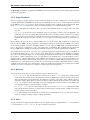
ImAFM™ reconstructs tip-surface force 𝐹 (𝑑) as a function of cantilever deflection 𝑑 = 𝑧 − ℎ, where the probe
height ℎ and the tip position 𝑧 are measured from a fixed position in the inertial reference frame where the sample
is at rest (the lab frame). ImAFM™ force measurement is fast enough such that one can assume constant probe
height ℎ at each pixel. This assumption will however break down when the feedback error signal is large and the
base is moving rapidly to compensate for a rapid change in surface topography. ImAFM™ makes no assumption
about where the surface actually is in relation to the probe height. This is in stark contrast to quasi static force
measurement methods, where one must assume a rigid tip and surface when calibrating the measurement of 𝑑 by
moving ℎ. In fact, ImAFM™ allows you to unambiguously define the location of the surface relative to ℎ, by
associating it with a distinct feature on the 𝐹 (𝑑) curve (see [Forchheimer-2012]).
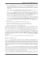
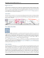
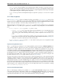
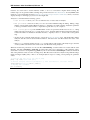
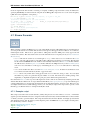
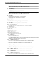
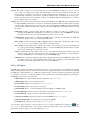
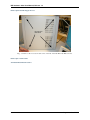
Fig. 3.1: The AFM detector measures cantilever deflection 𝑑. The probe height ℎ is adjusted while scanning. The
tip position in the lab frame is 𝑧 = ℎ + 𝑑.
Three basic methods are available for reconstructing 𝐹 (𝑑).
In the Force tab of the Force inspector settings panel, check the box to activate the desired
Reconstruction Method. You can use any combination of methods, and plot all results on the same plot.
Each method makes different assumptions described below. Click the method name to highlight it and view the
options for that method.
Polynomial The Polynomial method approximates the conservative tip-surface force (a function of tipsurface separation only) as a polynomial of finite degree 𝑁 in the cantilever deflection, 𝑑.
∑︀𝑁
𝐹 (𝑑) = 𝑗=1 𝑔𝑗 𝑑𝑗
A further assumption is that the force is zero when the tip is sufficiently far from the surface. Under these
assumptions we can find the 𝑁 polynomial coefficients 𝑔𝑗 , both odd and even coefficients, from the measured
spectrum of odd-order intermodulation products. The method is described in detail in [Platz-2012a], [Platz2013b].
Polynomial reconstruction has the following options:
3.1. Inspecting single pixels
21
IMP Software Suite User Manual, Release 1.2
• line style gives some plotting options for line type and thickness.
• Maximum IMP order is largest order of intermodulation product used in the determination of the polynomial coefficients. High order intermodulation products have lower signal level and depending on your
scanning conditions, they will disappear into the noise at some maximum order. The maximum order should
be set to the largest order IMP, which has a reasonable signal-to-noise ratio (SNR). You can judge the signal
the SNR by simply looking for contrast in the amplitude and phase images of any order IMP.
• Polynomial degree is the number of coefficients 𝑁 in the polynomial approximation of the force.
This number can not be greater than the maximum order intermodulation product in your spectrum.
• Assume localized force check-box activates the routine to determine the even polynomial coefficients. Zero force region sets the crossover deflection 𝑑0 , above which the tip-surface force is
assumed to be zero. The range is given in normalized coordinates, where -1.0 means closest to the surface,
and +1.0 means furthest from the surface. If you uncheck this fitting option you will reconstruct a force
curve which is an odd function of deflection, 𝐹 (𝑑 < 0) = −𝐹 (𝑑 > 0). The odd nature of the curve is due
to the fact that the intermodulation spectrum of odd-order products, is only able to reconstruct the polynomial coefficients, 𝑔𝑗 with odd 𝑗 (see [Platz-2013b]). If this odd 𝐹 (𝑑) curve shows a well developed zero
force region for 𝑑 > 𝑑0 , then we can safely neglect long-range forces and the assumption that 𝐹 (𝑑) = 0 for
𝑑 > 𝑑0 is well motivated. Move the slider to change 𝑑0 .
Model Fit The Model Fit method assumes that the tip surface force is described by a particular interaction
model, which has some number of parameters. The method performs a numerical optimization, adjusting the
parameters of the model, so as to best reproduce the measured frequency components of the tip-surface force.
The method is described in detail in [Forchheimer-2012], [Forchheimer-2013], [Platz-2012a]. Nearly any model
can be fit to the experimental data, so long as it can be coded on a computer. However, the solver will spit out a
solution and the software will give you a plot which looks like your force model - even if it is a lousy fit to your
data. Model Fit should always be used together with Polynomial or ADFS, in order to independently check if
the model makes sense. Model Fit also requires reasonable initial conditions for the solver to converge to a good
solution.
Model Fit reconstruction has the following options:
• line style gives some plotting options for line type and thickness.
• Choose model: selects the different force models that are programed in the software. You can also add
your own models to the software, as described in the advanced section on Programming your own Force
Models. The help icon
𝐹 (𝑑) for each model.
opens a window showing the functional form, a list of parameters, and plot of
• The table gives a listing of the parameters for each model, and the initial value for the numerical solver. If
the check-box is unchecked, the solver will not adjust that parameter and it will be fixed at it’s initial value.
Model Fit can be applied to every pixel in a scan to generate a paramter map, as described in Batch process
parameter maps and force volume data.
Amplitude Dependent Force Spectroscopy (ADFS) ADFS makes no assumptions about the particular form of
the force curve 𝐹 (𝑑) other than the force being zero for positive deflection, i.e. 𝐹 (𝑑) = 0 for 𝑑 > 0. The method
performs an inverse Able Transform on the 𝐹𝐼 (𝐴) curve, to reconstruct the conservative force 𝐹 (𝑑). The method
is described in detail in [Platz-2012b] , [Platz-2013a]. This method can be applied to create a force volume data
set from a scan data file, as described in Batch process parameter maps and force volume data.
Fast Polynomial A computationally efficient method to determine the polynomial coefficients of the conservative tip-surface force is described in [Platz-2013b]. The method is very fast compared to standard Polynomial and
Model Fit. The faster computation enables parameter mapping in real time, as scan data is acquired.
Live parameter mapping availabe as a script the pull-down menue:
LiveParameterMap.
Advanced -> Scripts ->
• Start will activate this feature and you can see the selected Parameter as a color map, painted during
the scan.
22
Chapter 3. Quantitative Analysis
IMP Software Suite User Manual, Release 1.2
• Show force curve when activated will plot the polynomial force curve at the center pixel of every scan
line. The force plot displays the selected parameter with a line or point on the force curve.
This type of parameter map can also be applied to scan data file, as described in Batch process parameter maps
and force volume data.
3.2 Analyzing lines and surfaces
At one pixel we can analyze data and make a curve of force or interaction energies as a function of cantilever
deflection or oscillation amplitude. These curves can be parametrized, for example by fitting the data to a particular
model of the interaction force. It is often very interesting to plot how the parameters change along a linear transect
of the image. This type of analysis can be made in real time with the Line inspector tool. You can also run
analysis of all pixels in a scan file to produce a color map image of each parameter. This later analysis is time
consuming and it can be run in a batch processing mode. The creation of these different types of parameter plots
and maps are described in the following sections:
3.2.1 Analyzing Linear Transects
If the Quantitative Analysis software is installed, selecting a line with the Line inspector tool activated will
open the Line Inspector panel. You will see a plot the amplitude and phase the intermodulation product
corresponding to the image showing when the line was selected. All data in each pixel along the transect line is
selected for analysis with the Model Fit method of force reconstruction.
• The Line Inspector panel gives a list of all selected lines in the left column. The color of the word
line in the list corresponds to the color of the linear transect in the Amplitude and Phase images.
• Right-click on the word line and choose Fit model from the menue. The currently active model will
be fit to the intermodulation spectral data along the transect line, and a plot will be generated showing how
each parameter of the model changes along the transect. Depending on the length of the line and the speed
of your computer, there may be some delay while the fitting is being performed at each pixel.
• You can automatically perform the fitting directly after the line is selected by checking the Fit model
check box at the bottom of the list of lines.
• Settings will open the Line Inspector Settings panel where you can activated different force
models, specify which parameters to adjust, and set the intial values of all parameters, as described in the
Model Fit section.
• You can test different models along the same linear transect: Simply change the model in the Line
Inspector Settings panel, then right-click on the word line and choose Fit Model. A fresh
plot of the parameters of the new force model will be made along this line. A new item is added to the list
with each fit that your perform. You can always go back to your previous plots by double-clicking on that
item in the list.
• Right-click on any an item in the list and chose Save to export the results of that fit to a text file. You can
also save the plot image by clicking the save icon in the Image Toolbar.
• Right-click on any item and select Remove to take it away from the list.
• Click on the small triangles to expand and contract the list of fits for each line.
• Right-click on either the Amplitude or Phase image with the Line inspector tool activated to remove
the line nearest to the right-click.
3.2.2 Parameter Maps
You can fit a force model to every pixel of a scan to create a parameter map, or color-coded image of the parameter values. From the Advanced pull-down menu, select Parameter map to open the Parameter map
creator. In this panel you may select the Model to fit to the data, and the initial values of all parametres, as
described in the Model Fit section. Because the generation of parameter maps using Model Fit is computationally
3.2. Analyzing lines and surfaces
23
IMP Software Suite User Manual, Release 1.2
intensive, it is often easire to use this interface off-line, so as not to overload the computer while scanning. Parameter maps can be generated while scanning using a method based on Fast Polynomial. You may PPLY either
method to your scan data files from the Batch process parameter maps and force volume data, where you can also
display the maps as 3D images projected on to the height data.
Analysis is controlled with the following options:
• scan direction allows you to choose either the trace or retrace data for analysis.
• CPU processes controls how many cores are used when multi-threading the fitting. Fitting a large
number of pixels will load the CPU and it may be too sluggish to use while scanning. Adjust this parameter
to find a good balance between time-to-output and response time of your computer.
• X-Y coarse-graining controls THE number of fits to be performed. If this factor is set to 𝑛 , fitting
will be performed on blocks of 𝑛 × 𝑛 pixels. If it is set to 1, all pixels will be analyzed. Increasing this factor
reduces the number of calculations and thus the time to output by a factor 𝑛2 , and it results coarse-grained
map.
• At the bottom is a list file names that are open in the Analyze Scan Data view. All checked files will be
analyzed, with the same model and initial conditions. The bar below each file indicates the status of the
analysis.
• click Start to begin the analysis and Abort to end the analysis. The results of the analysis (up to the time
of Abort) will be saved in the same folder as the scan file that is being analyzed.
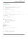
When the model fit is performed on a the scan file scan01234.imp, several new fiels are created with the same
filename. The files scan01234_p_name.png are image files with color-coded images of the parameter values.
Such a file is created for each parameter p_name in your model. The file scan01234.npz contains the numerical
data of the parameter values stored in one numpy array. This file can be loaded in to a Python script with the numpy
function numpy.load(file_name). Here is an example Python script for reading, and replotting the parameter
values:
# load the npz file in to the object pmap
pmap = np.load('scan01234.npz')
# extract and plot data for parampater 3, vmin and vmax are color bar limits
imshow(pmap['data'][3],vmin=0,vmax=5)
# display the colorbar
plt.colorbar()
24
Chapter 3. Quantitative Analysis
CHAPTER
FOUR
ADVANCED TOPICS
In order to comprehend some of the more advanced features in the IMP Suite, it is necessary to understand in
more detail how Intermodulation Measurement and Noise Calibration work. After this general discussion we
continue with sections devoted Programming your own Force Models. We explain how to use the the Data Tree
which organizes the analysis and allows you to view spectral data and extract it to an external text file. A section
is included on File Management, describing the different file types and where they are stored in the computer. We
describe how to move and re-arange the different Panels and Views and create your own custom screen layout.
Other advanced sections are given for the AFM scientist who wants to experiment with different types of multifrequency measurement and analysis. The IMP Suite has an Advanced Setup panel and a Drive Constructor
to configure the drive tones and measurement frequencies of the Multifrequency lockin Amplifier (MLA) ™. A
Stream Recorder is also included to record continuous streams of intermodulation data for analysis with your own
software. A Scripting Interface is also described which allows you to fully customize your multifrequency measurements with scripts that run in the IMP suite. We also document the ScanData python class which organizes
the multi-frequncy data. With the functions in ScanData you can write Python scripts that analyze an plot the data
stored in the scan files (e.g. scan01234.imp).
4.1 Intermodulation Measurement
Intermodulation AFM (ImAFM™) would not be possible without The Multifrequency Lockin Amplifier MLA™
(also known as the Intermodulation Lockin Analyzer ImMLA™, see [Tholen-2011]). The MLA™ comes in
different versions and it can be configured in many ways, but a typical configuration for ImAFM™ has the MLA™
is driving the AFM cantilever with two drive tones and analyzing the response at 32 intermodulation products of
the two drive tones, such that all frequencies in the response are located close to a high-Q resonance.
Intermodulation response should be zero when the cantilever is oscillating in air above a surface because the
freely oscillating cantilever is a linear system. When the cantilever is oscillating close to a surface and the tip is
interacting with the surface the cantilever oscillation becomes nonlinear, causing the generation of intermodulation
products of the two drive tones. Measuring both the amplitude and phase of the intermodulation products allows
one to reconstruct the nonlinearity, or the tip-surface force. Different force reconstruction methods are described
in the chapter on Quantitative Analysis.
The intermodulation measurement concept can be extended to multiple drive tones and the MLA™ can be configured to drive with more than two tones. A special Drive Constructor interface is provided for setting up the
multi-frequency drive and configuring the MLA™ to measure at the desired frequencies. Through a process
called tuning, the MLA™ and its accompanying software force all drive frequencies to be integer multiples (or
very nearly integer multiples) of one base frequency ∆𝑓 and this base frequency serves as a reference signal for
lockin measurement of the response. If all the drive tones are integer multiples of the base frequency, all of their
intermodulation products will also be at integer multiples of the base frequency.
Such multi-frequency signals are called frequency combs because their frequency representation, when plotted
as a power spectrum, looks like the teeth of a hair comb, with sharp spectral lines equally separated by the base
frequency ∆𝑓 . In the time domain the frequency comb is simply a periodic waveform with period 𝑇 = 1/∆𝑓 . A
general statement of the intermodulation measurement concept is the following: Drive a system with a frequency
comb and measure a response comb. The nonlinearity can be reconstructed from the difference between the
response and drive comb. The underlying assumption is that the response is periodic on the long time scale 𝑇
associated with the base tone.
25
IMP Software Suite User Manual, Release 1.2
The MLA™ has two different modes:
4.1.1 Time mode
Time mode down samples the response, averaging sequential samples to give an effective lower sampling frequency of. This improves the resolution to 16 bit and it allows for the transfer of every sample to the computer in
an uninterrupted stream (see :ref:stream-recorder-label). A DFT of this data stream will give you the entire intermodulation spectrum, up to the Nyquist frequency. This mode reveals all the mixing in your non-linear system.
However, the time mode has a latency between the end of the measurement period 𝑇 = 1/∆𝑓 and finish of the
calculation of the Fourier coefficients, which is the time require to DFT the window of sampled data. Even when
using the Fast Fourier Transform (FFT) algorithm to execute the DFT, this latency is too costly when scanning
over a surface. In such situations one uses the MLA™ in frequency mode.
4.1.2 Frequency mode
Frequency mode does the Fourier Analysis of many frequencies in parallel inside the MLA™ as the samples
are acquired. In frequency mode you get the full bandwidth of the MLA™ up to the Nyquist frequency set by
the sampling freqeuncy of the A/D converters in the MLA. The MLA™ performs 2𝑌 Fourier sums in real-time
at user-specified frequencies. These sums give you the Fourier cosine and sine coefficients, or the in-phase and
quadrature response. This response can be converted to amplitude and phase with some calculation, but often the
analysis of data is more conveniently done on complex numbers.
4.1.3 Feedback
The MLA™ has a feature specifically designed for AFM, where feedback is required to track the surface when
scanning. The amplitude of response at one dedicated feedback frequency is calculated inside the MLA™. This
amplitude is subtracted from a set-point amplitude, forming an error signal. A voltage proportional to this error
signal is sent to one of the output ports. In order to make the feedback more responsive, the MLA™ updates
the error signal 24 times in the measurement period 𝑇 = 1/∆𝑓 . The sections on Setup Feedback and Drive
Constructor give more information on how the configure the feedback and set-point.
4.2 Noise Calibration
A quantitative measurement of tip-surface force requires an accurate calibration of the cantilever. Noise calibration
uses the enhanced force sensitivity of a high Q resonance to measure the thermal equilibrium fluctuations of
cantilever deflection, and thereby extract the calibration constants of both the cantilever and the detector. The
method models the cantilever’s free dynamics as a simple harmonic oscillator; an accurate model for one cantilever
eigenmode, in a frequency band near resonance.
ImAFM™ also takes advantage of this enhanced sensitivity and high accuracy, using only signals near resonance
to reconstruct the force between the tip and the surface. Furthermore, ImAFM™ determines tip-surface force as a
function of the cantilever deflection at fixed probe height. Thus, both axes of the reconstructed force vs. deflection
curve (or force-quadrature vs. amplitude curve) rely on one and the same calibration. Quantitative measurement
with ImAFM™ is therefore completely independent of the scanner calibration [Platz-2012a] , [Forchheimer2012]. Noise calibration is performed for each cantilever at the start of the ImAFM™ session and it should be
redone if any adjustments are made to the detector. Calibration is easily done at any time during a session so it
can be frequently redone to check for consistency. Since the accuracy of quantitative ImAFM™ is traceable to
this one measurement, it is important to understand the physical ideas behind noise calibration.
Calibration in the field of AFM is traditionally discussed in terms of finding the spring constant 𝑘𝑠 associated with
the static (independent of time) deflection of the cantilever. Finding this one constant is sufficient to determine a
static force 𝐹 , which gives rise to the static deflection 𝑑,
𝑑=
26
1
𝑘𝑠 𝐹
Chapter 4. Advanced Topics
IMP Software Suite User Manual, Release 1.2
ImAFM™ is a dynamic method, where force is determined from cantilever motion 𝑑(𝑡). A linear relation between force and motion also exists for dynamic AFM if deflection is small in comparison to the cantilever length.
However, due to inertia and damping, the constant of proportionality is frequency dependent.
ˆ
ˆ 𝐹ˆ (𝜔)
𝑑(𝜔)
= 𝑘1 𝐺(𝜔)
ˆ called the transfer gain, and the hat denotes
The frequency dependence is contained in the dimensionless factor 𝐺,
an imaginary quantity, with the real part being the Fourier cosine component, and the imaginary part the sine
component at the angular frequency 𝜔. The complex, frequency-dependent quantity which relates each frequency
component of the force to the component of the motion at the same frequency, is called the linear response
function, and it is usually denoted 𝜒(𝜔).
ˆ
For the simple harmonic motion of each eigenmode of the cantilever,
ˆ
𝜔0 , 𝑄) = 𝑘1 [1 + 𝑖 𝜔𝜔0 𝑄 −
𝜒(𝜔)
ˆ
= 𝑘1 𝐺(𝜔;
𝜔 2 −1
]
𝜔02
√︀
Three parameters are needed to calibrate each eigenmode: The mode stiffness 𝑘, resonant frequency 𝜔0 = 𝑘/𝑚,
and the quality factor 𝑄 = 𝜔0 /𝛾, or alternatively: the mode stiffness, effective mass 𝑚 and viscous damping
coefficient 𝑚𝛾, where 2𝜋𝛾 is the width of the resonance in Hz. A complete calibration requires a fourth constant
that converts the measured detector signal in Analog-to-Digital Units (ADU) to actual cantilever deflection in
nanometers. This fourth constant is called the detector responsivity 𝛼 [ADU/m].
All four constants can be determined from one thermal noise measurement as described in [Higgins-2006]. Here
we give a somewhat different derivation of the method which is based on the idea that the cantilever is in thermal
equilibrium with the damping medium at temperature 𝑇 , and that the damping can be calculated using hydrodynamic theory. Thermal equilibrium and linear response allow us to use the fluctuation-dissipation theorem to
relate the power spectral density of fluctuations of cantilever deflection, to the imaginary part (the dissipative or
damping part) of the linear response function.
𝑆𝑑𝑑 (𝜔) =
2𝑘𝐵 𝑇
𝜔
2
ˆ
Im[𝜒(𝜔)]
ˆ
= 2𝑘𝐵 𝑇 (𝑚𝛾) 𝑘12 |𝐺(𝜔)|
[m2 /Hz]
2
ˆ
The simple harmonic motion gives us the functional form of |𝐺(𝜔)|
. We fit this function to the measured noise
peak at resonance, thus determining 𝜔0 and 𝑄. To get the magnitude of 𝑆𝑑𝑑 we require knowledge of the damping
coefficient 𝑚𝛾. Hydrodynamic theory and dimensional analysis is used to calculate the damping due to the
surrounding fluid (air, water, etc.) [Sader-1997].
𝑚𝛾 = 𝐿𝜇 Re Λ(Re)
Here 𝐿 is the length of the cantilever beam and Λ(Re) is a dimensionless hydrodynamic function of the Reynolds
number,
Re =
𝜌𝑏2 𝜔0
4𝜇
which is a dimensionless combination of the resonant frequency, the fluid density 𝜌 and viscosity 𝜇, and the width
of the cantilever 𝑏 . The hydrodynamic function Λ(Re) has been calculated for arbitrary rectangular beams with
length much larger than width, 𝐿 ≫ 𝑏 [Sader-1998]. However, the general theory applies to thin cantilevers of arbitrary shape, and Λ(Re) has been determined experimentally for the fundamental eigenmode of some commercial
cantilevers with non-rectangular shape [Sader-2012].
The deflection noise of the cantilever must be multiplied by the detector responsivity 𝛼 to convert it to the measured
quantity [ADU]. Since the cantilever noise is statistically independent from the detectors own noise, we can simply
add their noise powers to get the total noise power spectrum at the output of the detector,
𝑆tot (𝜔)[ADU2 /Hz] = 𝑆𝐷𝐷 + 𝛼2 𝑆𝑑𝑑 (𝜔)
We fit this expression to the measured data, with 𝛼, 𝜔0 , 𝑄 and 𝑆𝐷𝐷 as fitting parameters. Using the value of
𝜔0 determined from the fit, we can calculate the Reynolds number Re and thereby the hydrodynamic function to
determine the damping coefficient 𝑚𝛾. This coefficient, together with the value of 𝜔0 and 𝑄 determined from the
fit, give the mode stiffness 𝑘. Thus, thermal equilibrium linear response theory and the hydrodynamic damping
theory together give us all quantities needed to determine the linear response function of the cantilever and the
detector.
It is important to point out that the hydrodynamic damping function, and thereby the theoretical value of the damping coefficient 𝑚𝛾, depends on the mode shape and is therefore specific to the particular eigenmode. Calculations
show that the mode shape of the fundamental eigenmode of a long rectangular beam is particularly insensitive to
the Reynolds number. Higher eigenmode shapes are sensitive to Re [Sader-1998] and the mass of the tip placed
4.2. Noise Calibration
27
IMP Software Suite User Manual, Release 1.2
at the end of the cantilever. This calibration method is therefore applicable to the fundamental eigenmode and we
can expect it to be valid in different fluids, but its applicability to higher eigenmodes is questionable.
We should also stress that reconstructing force from the measured deflection over a wide frequency band, for
example from many harmonics of a single drive frequency, requires determination of the detector response function
𝛼
ˆ (𝜔). An ideal detector should have a flat (frequency-independent) response function up to it’s cut-off frequency
where it it will start to roll-off, or decrease with frequency to some power. However, real detectors do not always
behave in this ideal way, and the detector electronics can introduce frequency-dependent amplitude changes and
phase shifts over a wide frequency band. Since ImAFM™ works in a narrow band, we escape this difficulty and
we can expect accurate calibration and therefore accurate force reconstruction with the assumption of a frequencyindependent detector response function.
4.2.1 Note on sensitivity and accuracy
In the above text we emphasized that accuracy is higher when we base force reconstruction on the callibration of
high Q resonance. This notion of accuracy is rooted in physical understanding: We are better able to model the
force transducer and deflection detector in a narrow frequency band near a single eigenmode resonance, and thus
make a good calibration in this narrow band. We also argued that sensitivity is higher near resonance. Our notion
of sensitivity is independent of that regarding accuracy and it does not originate from theoretical understanding
of the physics of cantilever beams or opto-electronic detection. Sensitivity has to do with the signal-to-noise ratio
(𝑆𝑁 𝑅) of measurement.
The field of AFM has unfortunately adopted the term ‘inverse optical lever sensitivity’ (or invOLS) to describe the
constant 𝛼−1 which converts the measured detector signal (e.g. Volts) to nm of cantilever deflection. We use the
term responsivity for 𝛼 because it is actually the magnitude of a linear response function, and it does not tell us
anything about the 𝑆𝑁 𝑅 of the measurement. The sensitivity of the measurement is described by two quantities
which are displayed in the Calibration Result panel.
Thermal noise force is the random force due to collisions of the molecules in the damping fluid with
the cantilever. This random force has zero average value but the average of the force√︀
squared is not√
zero. The
thermal noise force is the square root of the power spectral density of force fluctuations 𝑆𝐹 𝐹 (𝜔)[fN/ Hz]. The
force noise power spectrum is independent of frequency, 𝑆𝐹 𝐹 = 2𝑘𝐵 𝑇 (𝑚𝛾) and this type of ‘white noise’ arises
whenever the damping force is simply proportional to velocity. With this thermal noise force we can calculate
a minimum detectable force 𝐹min , or the force measured with 𝑆𝑁 𝑅 = 1 in a given measurement time 𝑇
(measurement bandwidth 𝐵 = 1/𝑇 ).
For√example: The scan
thermal noise force
√ speed and image resolution dictate a pixel time of 𝑇 = 1 ms, and the√
is 𝑆𝐹 𝐹 = 22 fN/ Hz. The minimum detectable force at each pixel is therefore 𝐹min = 𝑆𝐹 𝐹 𝐵 = 696 fN.
This minimum force is the ‘signal’ which just equals the noise. A good measurement is typically characterized
by a signal which is many times the noise level, or 𝑆𝑁 𝑅 ≫ 1. Note that you must scan 4 times more slowly to
decrease 𝐹min by a factor of 2.
The detector Noise floor is the second quantitative measure of sensitivity. If the measurement time is short
or if you measure at frequencies away from the high-Q resonance, 𝑆𝑁 𝑅 is typically not determined by the actual
force noise of the cantilever in its damping medium, but rather by the electronic noise of the detector, 𝑆𝐷𝐷 .
We
detector noise as an equivalent deflection noise by dividing it with the detector responsivity,
√︁ express this √
equiv
−1
𝑆𝑑𝑑 = 𝛼
𝑆𝐷𝐷 . Here again we assume that the detector noise is independent of frequency in the band of
√︁
√
equiv
interest. If the pixel time is 𝑇 = 1 ms and 𝑆𝑑𝑑
= 150 fm/ Hz, the minimum detectable cantilever deflection
√︁
equiv
at each pixel would be, 𝑑min = 𝑆𝑑𝑑
𝐵 = 4.7 pm.
√︁
√︁
equiv
It is also interesting to express the detector noise as an Equivalent force noise 𝑆𝐹equiv
= 𝑘 𝑆𝑑𝑑
.
𝐹
√︁
√
equiv
For the example given above and 𝑘 = 40 N/m, we find 𝑆𝐹 𝐹 = 6 pN/ Hz , which, in a measurement time
equiv
𝑇 = 1 ms gives an equivalent minimum detectable force of 𝐹min
= 𝑘𝑑min = 0.19 nN. This would be the
minimum detectable force with the cantilever if the measurement were dominated by detector noise, as is often
the case for quasi-static force measurements.
Thus, sensitivity of the measurement is characterized by two quantities: The noise force of the cantilever, which
represents a fundamental limit, and the noise of the detector. One would like the detector noise to be as low as
28
Chapter 4. Advanced Topics
IMP Software Suite User Manual, Release 1.2
possible and a very useful way to compare different detectors is to use the ImAFM™ system to perform thermal
noise calibration on the same cantilever mounted in two different host AFMs. Since the cantilever force noise is
identical in each case, we can compare the ratio of the thermal noise peak, to the detector background noise, or
the Peak to flat ratio. The larger this ratio, the better your detection. It is also interesting to track this
number as you measure. If this ratio becomes smaller, it may mean that the detector is poorly adjusted, or there
may be some additional source of detector noise.
4.3 Programming your own Force Models
One powerful feature of ImAFM™ is the ability to test different tip-surface interaction models on the same data
set. Data is stored as the raw intermodulation spectrum at each pixel, which is a frequency-domain representation
of the tip motion. The Model Fit section of Force Reconstruction Methods describes how to use the IMP Suite
to fit this data to an a force model. This fit can be done at an individual pixel (see Force Inspector) , along a
liner transect (see Analyzing Linear Transects), or on an entire image (see Parameter Maps and Three dimensional
viewer). Several common force models are programed in the IMP Suite, and it is very easy to program your own
force model and have it appear in the IMP Suite.
Constructing a good and physically well motivated force model can be difficult. However, once you have a good
force model, programing it in the IMP Suite is simple. Some knowledge of the Python language is necessary (see
Python). Simply copy the examples.py file and give it a new name, e.g. my_force_model.py , keeping it in the
force_models folder. Edit the copy to create your own force model. The example.py file is well documented with
comment lines to help you understand the idea behind the Python code.
After you have finished with my_force_model.py, restart the IMP Suite. Your force model will be automatically
loaded and it will appear as an option in the Model pull-down menu. Note that any changes you may have made
to the examples.py file will not be saved, and upon restart, it will be returned to its original, default state.
4.4 Data Tree
The Data Tree panel is available from the Advanced pull-down menu. The panel can be docked in either the
scanning view or the analysis view, or both. This panel lists scans which are open in the analysis panel as well as
the current scan. Under each scan there is a list of all the pixels which have been selected with the Pixel inspector
tool. The color of the text for each pixel corresponds to the color of the cross marking the pixel in the image.
Under each pixel there is a list of the different force reconstructions done on that pixel.
Right click on a scan file name and select:
• Open shell here... to open a Python shell with an object called image containing all the data
stored in this scan file. The data id of the scan used by the data tree is given, along with a couple of useful
commands. The shell is for advanced users who will need the developer documentation to use this feature
effectively.
• Get calibration to open a dialog box with the calibration data stored with this scan file, or the Current
calibration at the time that the data file was closed.
4.3. Programming your own Force Models
29
IMP Software Suite User Manual, Release 1.2
• Save as ascii ... to open a dialog box where you can save all amplitude and phase data in ASCII
format. The save will create individual files in a new, empty folder. There will be one file for both amplitude
and phase at each of the measured frequencies, both trace and retrace. For example, when 32 frequencies
are measured, 128 data files will be created. If the image is 256 x 256 pixels, this corresponds to about
140Mbytes of data in tab-delimited text, with a carriage return at the end of each scan line.
The name of each file begins with a number which codes for the frequency. The number corresponds
to the index of the ‘k-array’ which stores the integers multiples of ∆𝑓 which give the frequency
values where amplitude and phase is measured (see Intermodulation Measurement). In the folder
there is also a file called metadata.txt which contains a list of integers in the array LO_IMP_KARRAY.
The number at the beginning of each file corresponds to the index of this array (zero being the first
element). The integer values stored in this array, times LO_DELTA_F, gives the frequency at which
the amplitude and phase is measured.
Right click on a pixel and select:
• Open shell here... to open a Python shell with an object called pixel containing the data relevant
to this pixel. The data id used by the data tree is given, along with a couple of useful commands. The shell
is for advanced users who will need the developer documentation to use this feature effectively.
• Delete removes the pixel from the data tree. The cross will also be removed from the image, and the plots
from the Fore Inspector panel. You can also remove any pixel by right-clicking close to that pixel in the
image when the Pixel inspector tool is selected.
• Save time data to text file to export the cantilever deflection vs. time during the time window
for this pixel. This data is is actually the inverse FFT of the spectral data taken by the MLA™, with some
zero padding to give appropriate sampling in the time domain.
• Save spectrum data to text file to export create the raw spectral data measured by the
MLA™ at this pixel.
• Save FI FQ data to text file to export the FI(A) and FQ(A) data for this pixel (see In-phase
and quadrature forces).
The check-boxes at each pixel and each force reconstruction controls plotting. Un-check to remove the cross from
the image or plot from the Force Inspector panel, without actually removing the data from the data tree. Checking
the box will show the plots again.
Pixels selected in the current scan will not be removed when a new scan is generated. When the scan moves passed
a selected pixel, the image no longer corresponds to the selected pixel. Selected pixels must be removed manually
in the current scan.
Clear All in the Force Inspector panel removes all selected pixels in all scans.
Right click on a force reconstruction and select:
• Open shell here... to open a python shell with an object called force containing the result of the
force reconstruction at this pixel. The data id used by the data tree is given, along with a couple of useful
30
Chapter 4. Advanced Topics
IMP Software Suite User Manual, Release 1.2
commands. The shell is for advanced users who will need the developer documentation to use this feature
effectively.
• Get fitted parameters to open a dialog box showing the fitted parameters when the Model Fit
method is used.
• Save Data to text file to export the force curve found using that reconstruction method.
4.5 Advanced Setup
The Advanced Setup view is initially selected in the Advanced pull-down menu. Thereafter the icon appears
on the right column, below the work flow icons. Selecting Advanced Setup again will uncheck the selection
and hide the icon. In this view you can control the drive for standard Intermodulation AFM using two drive tones,
set the feedback, and measure the response in real time.
Requested fields are the desired, or target values of:
• f1 [kHz] the frequency of drive 1
• f2 [kHz] the frequency of drive 2
• df the measurement bandwidth, df = abs(f2-f1) / n, where n = 1,2,3...
• A1 [%] the amplitude of drive 1, in percent of full output
• A2 [%] the amplitude of drive 2, in percent of full output
Actual show the values that you get, which depends on which algorithm you choose for frequency tuning.
4.5.1 Frequency tuning
Frequency tuning is key to performing measurmenets with the Multifrequency Lockin Amplifier (MLA)™
(MLA™). Tuning is the process of selecting the base tone df and the actual drive tones, so that they meet the
criteria for ImAFM™; that all frequencies are integer multiples df (see Intermodulation Measurement). There are
three different algorithms for tuning:
• None takes the requested frequencies and does not tune them at all. Without tuning, multi-frequency linear
response will be corrupted by Fourier leakage between drive tones and it is not possible to get an accurate
measurement of intermodulation.
• Rounding selects the closest frequencies to the requested values, such that all frequencies will be nearinteger multiples of one base frequency. Rounding gives a very small amount of Fourier leakage between
tones, but in almost all cases this leakage is well below the dynamic range of the measurement, and therefore
considered negligible. The phase error is corrected at the end of each measurement time (T=1/df), so there
should be no noticeable phase drift. With this algorithm there is considerable freedom in the choice of
frequencies.
• Integer is a more strict algorithm, where the condition of integer multiples is met exactly. This algorithm
gives no Fourier leakage between tones and no phase error, but it is more restrictive in the choice of the
possible values of df. You should use this algorithm when the MLA™ is synchronized to external frequency
generators. To avoid phase drift, you should make sure that the frequency of the external generator is an
exact integer multiple of df given in the IMP Suite, to as many significant figures as possible with your
generator.
The exact properties of these different tuning options have to do with the way in which frequencies are synthesized
and analyzed in the MLA™ which we do not discuss in detail here. It suffices to say that the small errors induced in
4.5. Advanced Setup
31
IMP Software Suite User Manual, Release 1.2
the Rounding algorithm are negligible for ImAFM™, and we recommend that you use this tuning. The automatic
setup uses this algorithm.
4.5.2 Setup Feedback
Before you engage a sample, and after you have made any changes to the drive configuration, you must setup the
feedback. Feedback for ImAFM™ is controlled by the amplitude of response at one of the frequencies measured
by the MLA™ (see Feedback section). For the basic two-frequency drive, feedback is run at frequency f1. With
the Drive Constructor you have more control over which frequency to set as the feedback frequency.
• Setup will adjust the feedback so that zero volts at the feedback output port corresponds to the given
set-point.
• Set-point is the desired response amplitude, given as a percentage of the free response amplitude. Adjusting the set-point to more than 100% will cause the probe to lift away from the surface. If you change
the set-point by a large amount, for example from 95% to less than 50%, it is a good idea to re-run Setup
feedback. The new set-point values are active as soon as they are entered in the field, and you hit return (or
tab).
The feedback port sends out an error signal for PID control of the Z-scanner. This feedback error signal is put
back in to the host AFM controller, in the place of the cantilever deflection signal. If the host AFM is set to contact
mode with the feedback set-point in the AFM software set at zero volts, the AFM’s PID control will adjust the Z
piezo to keep the error signal at zero volts, or the value of the set-amplitude. The feedback gains are adjusted in
the host AFM which is actually performing the feedback, using the error signal is calculated by the MLA™.
For example: If the set-point is set to 85%, the system will engage the sample until the response amplitude at
the feedback frequency drops to 85% of its free value. When this 85% condition is met, the MLA™ will have
zero volts at the feedback output. In our experience this amplitude feedback scheme is sufficient for tracking
most surfaces. When scanning large areas on rough surfaces, the feedback has to respond rapidly in order to
track the surface, and rapid adjustments of the cantilever base height are necessary. Force measurement is very
difficult when the cantilever base is rapidly accelerated by an over-active feedback. This acceleration gives rise to
additional forces on the tip which are not taken in to account in the reconstruction algorithms. Hence overactive
feedback means inaccurate force measurement. Improving feedback and actually incorporating the feedback
signal in to the force reconstruction is a subject for future research and development.
4.5.3 Measure
You can measure and plot the response in real time using two different modes:
• Run time mode starts the measurement of the response in the Time mode, and plots the sampled stream
of data in the time domain and its discrete Fourier transform (DFT) in the frequency domain. The discrete
data is plotted with a connected blue line. You will notice a jumping of the phase of the oscillation envelope
in the time-domain signal. This is normal as the data are analyzed and plotted in asynchronous chunks, and
not as one continuous stream. The DFT of the time-sampled data is however stable as each chunk as the
same sampling frequency and same number of samples.
• Run freq. mode starts the measurement of the response in the Frequency mode and plots the amplitude at the measured frequencies (vertical red bars) in the frequency domain, and the oscillation envelope in
the time domain (connected red lines)
• Stop will terminate the measurement. You must stop the measurement before you start other measurements, for example scanning a sample or taking stream data.
4.5.4 Units
You can select between displaying the cantilever response signal in Analog-to-Digital Units ADU , or in nanometers
nm. You must have a Current calibration in order to display in nanometers.
32
Chapter 4. Advanced Topics
IMP Software Suite User Manual, Release 1.2
4.5.5 Out of Range Error
The MLA™ is designed to handle signals within a ‘normal range’ for a ‘typical AFM’. Depending on your AFM
and our experiment, these normal range settings may need to be adjusted.
When the input signal exceeds the maximum, ‘clipping’ occurs inside the MLA™ and this induces harmonic and
intermodulation distortion in the spectrum. One way to avoid this problem is to simply attenuate the input signal.
Intermodulation Products provides attenuators to place at the SIGNAL IN port for this purpose. Note however
that a large signal coming from an AFM detector may bring the detector close to saturation, which also gives
harmonic and intermodluation distortion of the spectrum. Furthermore, a cantilever will behave with a nonlinear
restoring force when it is driven to very large response amplitude. One should be careful not to confuse these
sources of nonlinearity, which result in harmonic and intermodulation distortion of the free cantilever oscillation,
with harmonic and intermodulation due to a tip-surface force.
The output signal should also not exceed the maximum or be too small, in order to avoid distortion in the MLA™.
The requested drive amplitudes A1 [%] and A2 [%] are given in percent of full output (the actual values are
give in Digital-to-Analog units). The drive waveform coming from SIGNAL OUT port of the MLA™ can be
conditioned with external amplifiers or attenuators to suit the application. Intermal adjustments can be made inside
the MLA™ to give more or less output voltage. Contact Intermodulation Products regarding these adjustments.
4.6 Drive Constructor
The multiple tones in a frequency comb represent a periodic waveform in the time domain. The Drive Constructor
interface lets you configure the Mutifrequency Lockin Analyzer MLA™, creating the drive comb and choosing
the measurement frequencies. If you have a version of the MLA™ with more than two drive tones, for example the
IMP-24-24, there are endless possibilities for different drive waveforms and the question of which drive waveform
is optimal for a particular measurements is the subject of ongoing research. Before attempting to use the Drive
Constructor, you should read the section on Intermodulation Measurement.
The MLA™ versions are denoted IMP-X-Y, and they are constructed such that the X drive tones always overlap
with the and Y frequencies where response is measured. In other words, response is always measured at the X
drive frequencies and X ≤ Y. If you have the IMP-24-24 you can work with up to 24 frequencies which are
the same on both the drive and response sides. You can always work with fewer frequencies on the drive side
by simply setting the drive amplitude to zero at any drive frequency, thereby only measuring response at this
frequency.
4.6.1 Constructing a drive frequency comb
A Python scripting interface is built in to the drive constructor to help in the construction of drive frequency
combs. Using the interface requires knowledge of the Python programming language. A pull-down menu lists the
name of various Python scripts, stored in impdata/drive_setups/user_drive_scripts.py. These scripts are well
commented to help you understand how they work. You create a new script by changing the name of an old script,
and pressing Save. Similarly, Delete will kill the currently selected script.
The scripting interface has some useful functionality:
• Change font size with ctrl+Plus / ctrl+Minus or ctrl+Mouse wheel.
• Hit ctrl+Space for a list of reserved keywords
• A quick help and link to this manual appears by clicking the IMP help icon
4.6. Drive Constructor
.
33
IMP Software Suite User Manual, Release 1.2
Pre-defined variables
The following variables are defined in all scripts:
• f0 [Hz] and Q are the measured resonant frequency and quality factor stored in the Current calibration.
• nfreq_out and nfreq_in are the number of drive frequencies and response frequencies respectively. These
numbers will depend on the MLA™ firmware that you are running.
• f_sample is the sampling frequency [samples per second] of the MLA™.
Built-in functions
The following built-in functions are provided in all scripts:
• tune_integer(df) takes one argument, the target value of df . It returns a re-defined value of df that is commensurate with divisions of the MLA™ clock frequency, such that Fourier coefficients will be calculated for
perfect integer multiples of df. This function is equivalent to the integer button in the frequency-tuning
controls of Advanced Setup. You should use this tuning if you are synchronizing the MLA™ with other
instruments.
• tune_round(df, f0) takes two arguments, the target value of df and a desired frequency commensurate with
df (e.g. the resonant frequency of the cantilever) . It returns a re-defined value of df such that Fourier
coefficients will be calculated for near-integer multiples of df. This function is equivalent to the round
button in the frequency-tuning controls of Advanced Setup.
Required quantities
The script must set the values of the following variables:
• One (and only one) of the following which specifies the measurement bandwidth: Either df [Hz], T [sec],
or samples_per_pixel [integer]. (df = 1/T = samples_per_pixel/f_sample).
• An array of integers n giving the frequencies for both drive and response. The length of the array n must
be nfreq_in and the first nfreq_out entries are the drive frequencies. Alternatively, you can specify the
frequencies in an array called f. Set either n or f, but not both. (f=n*df).
• A real array a with the amplitude of all drive tones. The length of the array a must be nfreq_in. Amplitudes are given in DAU (digital-to-analog units). A helping function max_ampl() is useful in setting the
amplitude.
• A real array p with the phases of all drive tones. The length of the array p must be nfreq_out. Phases are
given in radians.
• A real number asf between zero and one. This amplitude scaling factor will set the peak amplitude of drive
signal. asf = 1 corresponds to maximum output voltage of the MLA™. The default value that you get if you
do not specify this variable is asf = 0.1. An error will appear in the debug window if asf is out of the range
[0,1]. asf = -1 it overrides this function (advanced users only!).
4.6.2 Synthesize and Configure
Synthesize Comb runs the script and plots the comb, as an amplitude-phase plot in the frequency domain,
and the waveform in the time domain. The MLA™ can be configured with this comb in one of two ways:
Configure Drive causes a voltage signal described by the synthesized frequency comb to be put at the signal
out port of the MLA™.
Configure Response adjusts the comb at the signal out port, such that the synthesized comb appears at the
signal in port. If the input signal is the detector of an AFM measuring the deflection of a cantilever the actual
cantilever motion will be that given by synthesized frequency comb. Configure Response assumes that a chain of
linear systems (actuator -> cantilever -> detector) is connected between the output and input ports of the MLA™
and it will not work properly when nonlinearity is present.
34
Chapter 4. Advanced Topics
IMP Software Suite User Manual, Release 1.2
4.6.3 Debugging a script
The Debug window allows you to test what is happening with your script. Error messages will appear in this
window and you can print any variable here using the dprint(var_name) statement in your script. The script
automatically prints relevant data for your comb in the Debug window.
4.6.4 Setting the feedback frequency
By convention, the MLA™ calculates the feedback error signal from the amplitude of the response at the frequency
located in the zeroth position of the n array (or f array). You should make sure that your script puts the frequency
at which you would like to run feedback in the zero position the n array. Note that the arrays do not need to
be sorted in any particular order, for example from lowest to highest frequency, but there must be a one-to-one
correspondence between the elements of the arrays which set the frequencies (n array), amplitudes (a array) and
phases (p array).
More information on feedback can be found in the section on Intermodulation Measurement (Feedback) and in
the section on Advanced Setup (Setup Feedback).
4.6.5 Useful Python code blocks
Some useful blocks of code for making frequency combs are described below. These code blocks are used in the
example scripts. You can copy and paste these in to your scripts.
Tune df close to 500 Hz and set the frequencies to consecutive integer multiples of df, centered as close as possible
to the resonant frequency f0:
df = tune_integer(500)
f1 =f0 - (nfreq_out / 2) * df #start freq of comb
n1 = round(f1/df) # integer closest f1
n = np.int_(arange(nfreq_out) + n1) # integer array of frequencies
Tune df closer to 500 Hz and set the frequencies to consecutive integer multiples of df, centered as close as
possible to the resonant frequency f0:
df = tune_round(500,f0)
f1 =f0 - (nfreq_out / 2) * df #start freq of comb
n1 = round(f1/df) # integer closest f1
n = np.int_(arange(nfreq_out) + n1) # integer array of frequencies
Exchange the frequency with the index mi, with the feedback frequency at position n[0]:
#put frequency near resonance as first frequency for feedback
mi=nfreq_out/2 #index of center of comb
n[mi], n[0], a[mi], a[0], p[mi], p[0] = n[0], n[mi], a[0], a[mi], p[0], p[mi]
Create an signal in the time domain, consisting of a rapidly oscillating component at the frequency f_bar and a
slowly modulated amplitude mod. Fourier transform and pick out the nfreq_out components close to f_bar and
set the amplitudes a and phases p:
N=2*int(2.*f_bar/df) #number of time samples, so f_max = 2*f_bar
t = arange(0.,1,1./N)/df
#construct signal x(t) in the time domain and FFT to get comb
mod = 0.1*sin(2.*pi*arange(N)/N) # the modulation function
x =(1.+ mod)*cos(2.*pi*f_bar*t) # x(t)
x_hat = fft.rfft(x)
# take components of comb, at frequencies given by n array
a = abs(x_hat[n])
asf = 0.1 # adjust peak amplitude
p = angle(x_hat[n])
4.6. Drive Constructor
35
IMP Software Suite User Manual, Release 1.2
Create an signal in the time domain, consisting of a rapidly oscillating component with a slowly modulated frequency f_bar*mod(t) . Fourier transform and pick out the nfreq_out components close to the center frequency
f_bar and set the amplitudes a and phases p:
N=2*int(2.*n_bar) #number of time samples, so f_max = 2*f_bar
t = (1./df)*arange(0.,1,1./N)
#construct signal x(t) in the time domains
x = cos(2. * pi * ( f_bar * t
delta_f /(4*pi*df)*sin(2*pi*df*t)))
# FFT to get frequency comb
x_hat = fft.rfft(x)/(N/2.)
a = abs(x_hat[n])
asf = 0.1 # adjust peak amplitude
p = angle(x_hat[n])
4.7 Stream Recorder
When scanning a sample, the MLA™ process end-of-line (EOL) and end-of-file (EOF) triggers and lockin data is
stored at pixel locations in a scan file. The stream recorder ignores all triggers and stores data as one continuous,
uninterrupted stream. This mode is quite useful for taking data when the AFM probe slowly approachs and
retracts from a surface. The data stream can be stored in either time mode or frequency mode (see Intermodulation
Measurement).
• Start will start the stream record. Click again to Stop. If the Autosave box is checked in the Status
Banner, each run of the stream recorder will result in a file being saved in the session folder. The file name
has the form record01234 where the number is automatically incremented. In Time mode the files will have
the .std extension, and in Frequency mode the files will have the .imp extension (see the File Management
section for more information on file types). Unchecking the Autosave box will result in no data being
saved.
• Mode selects weather the data is stored in Time mode or Frequency mode. In either mode all data is saved
as a continuous stream without any breaks or gaps in the data.
• Plot controls only which data is being plotted and does not effect the saving of data. You can adjust
the number of points to be plotted in the past number of seconds. The check boxes enable plotting of the
amplitudes (or amplitude and phase in the polar plot) at the different frequencies listed.
Note that in the Time mode the response at all frequencies in the comb can be examined by analyzing stream data
with the Fast Fourier Transform. A script called PlotTimeMode (see Scripting Interface) is provided which gives
a simple GUI inteface for plotting and extracting time-mode data taken with the stream recorder. Below we give
an example which can be a useful starting point for your own analysis scripts. The script can be copied to a new
filename.py, modified and run, for example in the iPython shell.
4.7.1 Example script
This script reads a time-mode stream data file (.std file) and parses it in to time windows or ‘beats’, on which the
signal is periodic. Each time window is assigned an index (the beat index) and the terminal asks for the beat index
on which you want to perform analysis. The script extracts that beat from the data file, and simply plots both time
data and the frequency data. Note that you must input the path to the IMP Suite on your computer, and the path to
the .std file that you want to analyze:
import matplotlib.pyplot as plt
import numpy as np
import sys
36
Chapter 4. Advanced Topics
IMP Software Suite User Manual, Release 1.2
# Path to IMP Suite
suitepath = '/Users/david_haviland/IntermodulatorSuite'
sys.path.append(suitepath)
from StreamRecorder import stdfile
# Path to stream recorder file in time-mode
recorder_path = 'path_to_file.std' # full path to recorder file in .std format
print "loading file", recorder_path
sf
= stdfile.stdfile(recorder_path,b_raw=False,do_scale=False)
# Read metadata from file
fs = sf.freq_samples # Sampling frequency, Hz
f1 = sf.f1 # First drive frequency, Hz
f2 = sf.f2 # Second drive frequency, Hz
# Calculate number of samples to avoid Fourier leakage
n_samples_beat = int(np.round(fs/abs(f2-f1))) # Number of samples in one beat
t = 1./fs*np.arange(n_samples_beat) # Time axis for plotting
df = fs/n_samples_beat # Frequency resolution
freqs = df*np.arange(n_samples_beat/2+1) # Frequency axis for plotting
# Index each beat in the stream
ii_s = np.arange(0,sf.n_samples,n_samples_beat)[:-1] # remove last since it might not be complete
# Loop through all beats and read max value
beats_to_plot = 1000
if len(ii_s)<=beats_to_plot:
ii_plot = ii_s
else:
skip = float(len(ii_s))/beats_to_plot
ii_plot = np.int_(skip*np.arange(beats_to_plot))
peak = np.zeros(len(ii_plot))
for i,beat_i in enumerate(ii_plot):
if i%100==0:
print "Beat %i / %i"%(beat_i, len(ii_s))
# Read data
i_start = ii_s[beat_i]
data = sf.get_samples(i_start,n_samples_beat)
peak[i] = max(data)
# Plot
plt.figure(1)
plt.clf()
plt.plot(ii_plot,peak)
plt.xlabel("Beat index")
plt.ylabel("Peak value [ADU]")
plt.show()
# Ask terminal for beat number, then data from that beat
n = -1
while n == -1:
s = raw_input("Enter beat index to plot: ")
try:
n = int(s)
except ValueError:
print "Input must be an interger"
data = sf.get_samples(ii_s[n],n_samples_beat)
data_fft = np.fft.rfft(data)/len(data)
# Plot
4.7. Stream Recorder
37
IMP Software Suite User Manual, Release 1.2
plt.figure(2)
plt.subplot(211)
plt.plot(t,data)
plt.xlabel("Time [s]")
plt.ylabel("In [ADU]")
plt.subplot(212)
plt.semilogy(freqs*1e-3,2*abs(data_fft))
plt.xlabel("Frequency [kHz]")
plt.ylabel("Amplitude [ADU]")
plt.show()
4.8 Scripting Interface
The IMP Suite comes with a python scripting interface with which you can develop you own multifrequency AFM
methods and customize the IMP Suite to your particular measurement needs. From this interface you can access
all the classes and functions used by the IMP Suite for data acquisition, storage, plotting, and analysis. To take full
advantage of the possibilities that this interface allows and to develop your own measurements, you will need to
learn the Python programing language, and become familiar with the structure and functionality of the IMP Suite
as described in the developer documentation.
Intermodulation Products provides a variety of scripts which can be modified and saved with a new name. All
scripts stored in the folder IMP_sessions_and_settings/settings/scripts will be loaded when the IMP Suite starts,
and they will appear in Advanced pull-down menu under Scripts. To run the script, simply select it from the
menu. Reload scripts will close all open scripts are reload the currently saved script.
The file Examples.py contains several different classes, each containing a script with different functionality. These
scripts demonstrate how to make a GUI or step a quantity while scanning. You can expand on these scripts to add
GUI elements and controls, or simply edit the values in the Python code, reload the script, and run it. These scripts
serve as a starting point to develop your own measurement methods.
Some useful scripts currently available are:
4.8.1 RecorderAnalysis.py
PlotTimeMode opens a GUI for viewing and extracting sections of a Stream Recorder file. Run the script, press
Open and select a previously recorded .std file containing stream data taken in Time mode. The script will parse
the time stream to a series of ‘beats’ , or time windows 𝑇 given by the inverse of the measurement bandwidth
𝑇 = 1/∆𝑓 , assigning a ‘beat index’ to each window. A plot shows the maximum value of the oscillation envelope
in each beat. You can adjust the time window to include more than one beat, thereby reducing the measurement
bandwidth and thus the noise. The time window is shown in the lower plot. Export All will export the entire
recorder file and Export zoom will export only the selected window (lower plot) to an ASCII format file. A
Fast Fourier Transform (e.g. FFT) of this data will give the response spectrum at the selected time window.
4.8.2 LiveParampeterMap.py
LiveParameterMap runs an experimental new method for extracting polynomial force curves which is computationally very efficient, so that the curves are analyzed and parameter maps are made in real time, as the AFM
scans. The method was developed and implemented by Daniel Forchheimer, starting from a theory worked out by
Daniel Platz [Platz-2013b]. Choosing this script opens a GUI which allows you to choose ways of parameterizing
the conservative tip-surface interaction force. A map of these parameters is created in real time and a force curve
showing the extracted parameter can be plotted. The force curve is taken at one location (center) of the fast-scan
axis and the plot is updated at the line frequency.
38
Chapter 4. Advanced Topics
IMP Software Suite User Manual, Release 1.2
4.9 Scan Data
The IMP Software Suite stores data from a scan, including all relevant metadata, in one compact file with the file
extension .imp (e.g. scan01234.imp). The ScanData class manages the storage and retrival of the data. If you
want to write your own Python scripts to analyize multifrequency data taken with the IMP Software Suite, you
will need to use the ScanData class. The documentation below was auto generated from the doc strings in Python
code at the time this manual was compiled. You can always see the documentation of the actual class version that
you are using in the Python code itself, using auto-complete with any good Python API (Advanced Programming
Interface).
4.9.1 Using the ScanData class
Below are some example scripts which demonstrate how to load the ScanData class and get at the data stored in
the scan file.
Can we make some kind of structure like matplot lib to exand tp see soruce code or result of run?
example of how to imshow the phase of particular frequency.
example of how to exchange the free oscillation with a particular pixel.
4.9.2 ScanData Class
class Scanner.ScanData.ScanData(args=[])
Handels the storage and retreval of data from the scan file (e.g. scan01234.imp).
This class is designed to be easily extendable and new functions will be added as the IMP Suite grows.
Most functions in this class fall in to one of two groups:
• Use append_ and reset_ to prefix functions for managing data in a list.
Use when you want to save the history which changes during the scan. The final member of the list
is often called the ‘current’ data. append_ function adds to the end of a list. reset_ function clears the
list to length zero and adds a new initial element.
• Use get_ and set_ to prefix functions which get data and set data respecitvely in the ScanData
class.
This can be the raw image data at any pixel, or meta data such as the calibration or free oscillation.
To Do:
• clean our not used functions.
• change invOLS to invOLR everywhere
append_lo_change_linenrs(val)
Append the list of change_linenrs values
append_lo_delta_f(val)
Append the list of delta f values
append_lo_drive_amplitudes(ar)
Append the list of drive_amplitudes
append_lo_drive_karray(ar)
Append the list of drive_karray values
append_lo_drive_phases(ar)
Append the list of drive_phases
append_lo_feedback(ar)
Append the list of feedback
4.9. Scan Data
39
IMP Software Suite User Manual, Release 1.2
append_lo_free_oscillations(ar)
Append the list of free_oscillation
append_lo_imp_karray(ar)
Append the list of imp_karray values
append_lo_samples_per_pixel(val)
Append the list of samples_per_pixel values
append_lo_sampling_freqs(val)
Append the list of sampling_freq values
append_lo_scan_rates(val)
Append the list of scan_rate values
append_lo_tip_Vac(val)
Append the list of tip AC voltage values
append_lo_tip_Vdc(val)
Append the list of tip DC offset values
append_setpoint(setpoint, linenr=-3)
Append a setpoint to the setpoint history.
The optional linenumer argument can also be negative linenr = -1 : changed in last image linenr = -2 :
during setup linenr = -3 : unknown point of time
equal_array(ar1, ar2)
Checks to see if two arrays have equal length.
Parameters
• ar1 – np.array
• ar2 – np.array
Returns True or False
Return type bool
get_Q()
Returns dimensionless quality factor.
Return type float64 [-]
get_change_linenr()
Return the current value of change_linenrs, i.e. the last in the list
get_delta_f()
Return the current value of delta f, i.e. the last in the list
get_drive_amplitudes()
return the current (i.e. latest) drive amplitudes
get_drive_karray()
Return the current value of drive_karray, i.e. the last in the list
get_drive_phases()
return the current (i.e. latest) drive phases
get_external_filename()
get_feedback()
Return the current value of feedback, i.e. the last in the list
get_free_oscillation()
Return the current value of free_oscillation, i.e. the last in the list
get_free_oscillations_complex(num=-1)
40
Chapter 4. Advanced Topics
IMP Software Suite User Manual, Release 1.2
get_imp_karray()
Return the current value of imp_karray, i.e. the last in the list
get_imp_str_list(mode=-1)
Returns a list of imp strings, containing e.g. ‘Drive1’, ‘Drive2’, ‘IMP3L’ etc. Without further options,
the strings are returned as saved in the corresponding ImageData. With mode = 0, same as mode==-1,
but if strings are empty automatically mode 2 With mode = 1, same as mode==-1, but if strings are
empty automatically mode 3 With mode = 2, strings of the imp-ks are returned, e.g. ‘k = 345’. With
mode = 3, strings as defined in ScannerPanel are returned, depending on the lockin scheme.
get_internal_imp_str_list()
get_invOLS()
Returns resopnsivity of optical lever.
Return type float64 [nm/ADU]
get_k()
Returns catilever eigenmode stiffness.
Return type float64 [N/m]
get_loaded_filename()
Filename that was used when loading the ScanData from disk
get_lockin_scheme()
Gets the lockin scheme used for scanning, currently returning 0, 1 or 2
get_metadata_ascii()
Return all metadata as a string new-line separated string
Strategy for all following data entries: IDENTIFIER[UNIT]: DATA
get_original_filename()
get_p_detector_white()
Returns ???what is detector white
Return type float64 [???]
get_p_thermal()
Returns ??? what is p_thermal
Return type float64 [???]
get_params_dict()
get_resolution()
get_resonance_frequency()
Returns resonance frequency
Return type float64 [Hz]
get_samples_per_pixel()
Return the current value of samples_per_pixel, i.e. the last in the list
get_sampling_freq()
Return the current value of sampling_freq, i.e. the last in the list
get_scan_rate()
Return the current value of scan_rate, i.e. the last in the list
get_scan_size_x()
Returns scan size in the fast-scan direction x.
Return type float64 [meters]
4.9. Scan Data
41
IMP Software Suite User Manual, Release 1.2
Note: The scan size is determined by the host AFM and must have been entered in manually in the
IMP suite. Automatic reading for some AFM’s is under development.
get_scan_size_y()
Returns scan size in the slow-scan direction y.
Return type (float64) [meters]
Note: The scan size is determined by the host AFM and must have been entered in manually in the
IMP suite. Automatic reading for some AFM’s is under development.
get_setpoint()
Return the current value of setpoint, i.e. the last in the list
The linenumber of the setpoint chnage is not returned.
get_starttime()
get_tip_Vac()
Return the current value of tip AC voltage, i.e. the last in the list
get_tip_Vdc()
Return the current value of tip DC offset, i.e. the last in the list
given_list_is_empty(lst)
Returns True if list is [] or only has elements of type ‘’, otherwise returns False
has_calibration()
has_equal_params(other)
isEqual(other)
load_from_file(filename)
load_h5_file(filename)
load_legacy_imp_file(filename)
Loads data from binary file in .imp format
purge_parameters()
Purges the parameter history lists.
All except for the last entries are removed from the parameter lists. This is useful when a new image
is saved then the parameter history of the previous image should be removed. Only the last value in
each list is kept as the initial parameter for the new image.
reset_lo_change_linenrs(val)
Reset the list of change_linenrs values and initialize it with one element with value val
reset_lo_delta_f(val)
Reset the list of delta f values and initialize it with one element with value val
reset_lo_drive_amplitudes(ar)
Reset the list of feedback values and initialize it with one element with array ar
reset_lo_drive_karray(ar)
Reset the list of drive_karray values and initialize it with one element with karray ar
reset_lo_drive_phases(ar)
Reset the list of feedback values and initialize it with one element with array ar
reset_lo_feedback(ar)
Reset the list of feedback values and initialize it with one element with array ar
reset_lo_free_oscillations(ar)
Reset the list of free_oscillation values and initialize it with one element with array ar
42
Chapter 4. Advanced Topics
IMP Software Suite User Manual, Release 1.2
reset_lo_imp_karray(val)
Reset the list of imp_karray values and initialize it with one karray ar
reset_lo_samples_per_pixel(val)
Reset the list of samples_per_pixel values and initialize it with one element with value val
reset_lo_sampling_freqs(val)
Reset the list of sampling_freq values and initialize it with one element with value val
reset_lo_scan_rates(val)
Reset the list of scan_rate values and initialize it with one element with value val
reset_lo_setpoints(val)
Reset the list setpoints values and initialize it with one element, a value val
reset_lo_tip_Vac(val)
Reset the list of tip AC voltage values and initialize it with one element with value val
reset_lo_tip_Vdc(val)
Reset the list of tip DC offset values and initialize it with one element with value val
save_to_ascii(filename=None)
Export to a collection of generically named ascii-files in the directory ‘dirname’.
Creates a separate subdirectory for the scan and separate files for each amplitude and phase image for
easy import into Matlab or similar.
If dirname==None (default) the directory is automatically named after the scanData file
save_to_file(filename)
save_to_h5(filename)
save_to_legacy_imp_file(filename)
Saves data as binary file in .imp format
set_Q(Q)
Parameters Q – float64 [-] dimensionless quality factor.
set_calibration_flexural(kwargs)
set_calibration_torsional(kwargs)
set_change_linenr(val)
Set the current value of change_linenr, i.e. the last in the list, to new a new value val
set_delta_f(val)
Set the current value of delta_f, i.e. the last in the list, to new a new value val
set_drive_amplitudes(ar)
resets the list of drive amplitudes and appends the given array
set_drive_karray(ar)
Set the current value of drive_karray, i.e. the last in the list, to a new karray ar
set_drive_phases(ar)
resets the list of drive phases and appends the given array
set_external_filename(str)
set_feedback(ar)
Set the current value of feedback, i.e. the last in the list, to new a new array ar
set_free_oscillation(ar)
Set the current value of free_oscillation, i.e. the last in the list, to new a new array ar
set_imp_karray(ar)
Set the current value of imp_karray, i.e. the last in the list, to new a new karray ar
set_invOLS(invOLS)
4.9. Scan Data
43
IMP Software Suite User Manual, Release 1.2
Parameters invOLS – float64 [nm/ADU] responsivity of optical lever.
set_k(k)
Parameters k – float64 [N/m] cantilever eigen mode stiffness.
set_nr_drive_freqs(nr)
set_original_filename(str)
set_p_detector_white(p_detector_white)
Parameters p_detector_white – float64 [???] ???what is detector white
set_p_thermal(p_thermal)
Parameters p_thermal – float64 [???] ???what is p_thermal
set_resolution(i_x, i_y)
set_resonance_frequency(f0)
Parameters f0 – float64 [Hz] resonance frequency.
set_samples_per_pixel(val)
Set the current value of samples_per_pixel, i.e. the last in the list, to new a new value val
set_sampling_freq(val)
Set the current value of sampling_freq, i.e. the last in the list, to new a new value val
set_scan_rate(val)
Set the current value of scan_rate, i.e. the last in the list, to new a new value val
set_scan_size_x(value)
Parameters value – float64 [meters] scan size in the fast-scan direction x
set_scan_size_y(value)
Parameters value – float64 [meters] scan size in the slow-scan diretion y.
set_starttime(val)
set_tip_Vac(val)
Set the current value of tip AC voltage, i.e. the last in the list, to new a new value val
set_tip_Vdc(val)
Set the current value of tip DC offset, i.e. the last in the list, to new a new value val
swap_calibration_parameters()
4.10 File Management
The IMP suite is kept in different places, depending on your computer system. In Windows, it is installed in
c://Program Files/IntermodulatorSuite. Users do not need to care about this folder as it contains only static
files which should be installed from an installer. All dynamic files that are changed when you change settings in
the IMP Suite, store data, save a script, etc., are stored in the folder c://IMP sessions and settings. This folder
has the following sub-folders:
Moving data to another computer
To transport your data to another computer for analysis, be sure to first import the host AFM data (i.e. height
image data) in to your session folder using the Session Overview. Then simply copy the entire session folder
to another computer with the IMP Suite installed. When you perform analysis on another computer, all
newly created analysis files will be added to the session folder.
44
Chapter 4. Advanced Topics
IMP Software Suite User Manual, Release 1.2
/sessions This folder contains session folders. Each time you start the IMP Suite a dialog box opens to create a
new, or add to an existing session folder. The default name of the new session folder is the date, but you
have the option to append a session name to the date. When Autosave is checked (see Status Banner), data
is automatically stored in the session folder: scan files, calibration files, stream files, the session log, etc..
When you analyze data to create new files or import host AFM data files, the default behavior is to always
store everything in the session folder.
/settings This folder contains many files that are changed dynamically by the IMP Suite and configuration files
for different AFMs. Normal users do not need to work directly with these files but advanced users may want
to modify them. If these files become corrupt, they can be discarded and the IMP Suite will automatically
recreate the files with their default values on the next start of the IMP Suite. The settings folder has several
sub-folders:
/calibration Contains several text files with the calibration constants for each type of cantilever programmed in the IMP Suite, including those created by a user. There is also a file fluid.txt containing
the density and viscosity of the various fluids that you may want to work in.
/configurations Contains files for configuring the IMP Suite to work with your particular host AFM. The
normal user will not need to be concerned with these files.
/drive_setups Contains the file user_drive_setups.py which is a Python file containing the scripts for the
Drive Constructor, both example scripts and user-constructed scripts.
/force_models Contains Python files with the force models. You can add your own force model files here
by copying and modifying /example.py. When you restart the IMP Suite this file will be re-loaded
and your model will appear as a new force model.
/scripts Contains Python scripts which can be sued to control different measurement schemes and create
different modes. This is for advanced users who will require some knowledge of the basic Python
objects in the IMP Suite. A few examples are given in /Examples.py
/config.ini This is the main configuration file which is dynamically changed by the IMP Suite. The normal
user will not need to be concerned with this file. If it becomes corrupted, it can be deleted and a new
file will be created with default values upon restart of the IMP Suite.
4.10.1 File Types
The IMP Suite generates files with a name indicating the type of file, followed by an automatically incremented
5-digit counting number (denoted ‘01234’ below). You are free to append an underscore followed by any valid file
text after this counting number (e.g. scan01234_my-file-text.imp). You may experience problems keeping track
of your files if you remove or modify this number or the type name before it. The following files are generated by
the IMP Suite and stored in a session folder:
• calib01234.txt noise data and fitted calibration parameters (see Calibration).
• calib01234.png image of plot in calibration view.
• sweep01234.txt frequency sweep data (see Frequency Sweep).
• sweep01234.png image of the frequency sweep plot.
• scan01234.imp data for one scan, including the current calibration, in HDF5 format.
• recorder01234.imp continuous stream of data taken in frequency mode (see Stream Recorder).
• recorder01234.std continuous stream of data taken in time mode.
• scan01234_model.npz parameter map data for the fitted model (see Parameter Maps).
• scan01234_p-name.png color map image of the parameter p-name.
• sessionlog.txt chronological session log (see Session Logbook).
in the
You can always export an image of any plot that you see on screen by clicking the save image icon
Image Toolbar, which will bring up a save dialog box with several file format options. You can also export raw
data and the results of analysis to a text file using the Data Tree .
4.10. File Management
45
IMP Software Suite User Manual, Release 1.2
4.11 Panels and Views
All views, or screen layouts, have a main panel to which auxiliary panels can be docked. Several views are predefined and they appear when clicking icons in the left column symbolizing the The Work Flow. Icons for the
advanced panels appear when selected in the advanced pull-down menu. To removed the advanced icons, select
again in the pull-down menu.
Different panels appear when you click Settings buttons, or they can be chosen from the Analysis pulldown menu. You can add these panels to the views, or rearrange the panels in a view according to your desire.
Movable panels have a shaded grab-bar on top, where the panel name is located. These panels can be free-floating,
or you can dock them to a particular view.
• To un-dock a panel, click-and-drag the panel bar. Release when it is un-docked and it will be free-floating.
A double-click on the panel bar will also un-dock the panel.
• To dock a panel, click-and-drag the panel bar of a free-floating panel and panel position icons will appear.
Move your mouse cursor to the desired dock location on the icon, and your screen will show a shaded area.
Upon release the panel will dock to the shaded area.
46
Chapter 4. Advanced Topics
CHAPTER
FIVE
INSTALLATION
5.1 Install Software
The IMP Software Suite is installed with a standard installer. When you install the software, you agree to the
terms of the IMP license. The IMP software Suite can be run on the same computer as the host AFM, or on a
separate computer. It is advantageous to run the IMP Suite on a modern computer with a multi-core processor,
especially when analyzing full images to make Parameter Maps.
If the IMP Suite does not detect the The Multifrequency Lockin Analyzer™ (MLA™) upon starting, it will open
up in analysis mode. In analysis mode you can plot and analyze data taken previously, but you can not take data.
You are free to install the software on as many seperate computers needed to analyze your data. To take data you
mast start the IMP Suite when connected to the MLA™ and a host AFM, as described below.
5.2 Install Hardware
Connecting the hardware the first time requires some effort. However, if things are configured nicely, one or two
hardware switches is all that is needed to switch between the normal configuration of your host AFM and the
ImAFM™ configuration. The MLA™ is connected to the host AFM via a signal access module (SAM) provide
by Intermodulation Products or your AFM supplier. The MLA™ is connected to a computer running the IMP
Suite via Ethernet, either the same computer used by the host AFM, or a seperate computer.
5.2.1 Connection to computer
The IMP Suite will open analysis mode when it does not detect an MLA™ connected to the computer. To establish
the connection between the computer and the MLA™ you must first perform the steps below. After this procedure
the detection will be automatic. The instructions given below are for Windows 7.
1. Connect a standard Ethernet cable between the MLA™ and the computer.
2. Go to Control Panel -> Network and Internet -> Network and Sharing Center.
3. Locate the network adapter: In the left panel choose Change adapter settings. To identify
which adapter corresponds to the Ethernet card connected to the MLA™, turn off the MLA™. There should
be a red cross on the adapter icon with the text Network cable unplugged. About one minute after
the MLA™ is turned on the red cross will disappear and the text changes to Unidentified network.
4. Configure the MLA adapter: Right click again on the MLA adapter and choose Properties. Select Internet Protocol Version 4 (TCP/IPV4) and click Properties. Click Use the
following IP address and fill in the following
IP address: 192.168.42.1
Subnet mask: 255.255.255.0
5. Check the adapter: At this point the internet connection between the MLA™ and the computer should be
established. To test the connection you can ping the MLA™. In a Windows terminal window type ping
192.168.42.50. The MLA™ should respond with something like:
47
IMP Software Suite User Manual, Release 1.2
Pinging 192.168.42.50 with 32 bytes of data:
Reply from 192.168.42.50: bytes=32 time=1ms TTL=128
5.2.2 Connection to host AFM
The general connection scheme is shown the diagram above. The cantilever drive, detector, feedback and trigger
signals must be routed through the MLA™. This routuing may be with with BNC cables to the font pannel of
the MLA™, or with a composite cable to the AUX connection of the back panel of the MLA™. On some AFMs
a separate Signal Access Module (SAM) is required. Intermodulation Products provides dedicated SAMs for a
few common AFMs to easily toggle between the normal function of your host AFM and ImAFM™. On other
AFMs, notably Asylum and JPK, one connects BNC cables directly to the controller and changes signal routing
using software activated switches. You can get a script from Intermodulation Products to automatically perform
the signal routing. Detailed instructions are given below for different AFM’s. Contact Intermodulation Products
to find out what solutions exist for your particular AFM <[email protected]>.
5.3 Set AFM Type
In the IMP Suite, under the Advanced pull-down menu, select Setup AFM. A dialog box appears with a pulldown menu to choose your AFM type. This option will only appear when the IMP Suite detects the MLA™ and
starts in full mode, ready for taking data. The settings for the various AFM types are stored in the folder IMP
Sessions and Settings/settings/configurations. These files contain information about triggers, over-scan factors,
and more. Advanced users can use the files in this folder as a template to make their own custom_afm.ini settings
file. When the software is restarted, a new custom_afm settings will appear as a choice in the pull-down menu.
If your AFM type does not have a configuration file, contact Intermodulation Products for help in making a
custom configuration file <[email protected]>.
5.3.1 Working without triggers
Nearly all AFM’s have some kind of access to the end-of-frame (EOF) and end-of-line (EOL) triggers. If the
EOF trigger does not exist, it is still possible to manually start the ImAFM™ scan when the host AFM scan starts.
However, after several scans a manual restart is needed to re-sync the frames. If the EOL trigger does not exist,
48
Chapter 5. Installation
IMP Software Suite User Manual, Release 1.2
it is also possible perform ImAFM™ but in this case one needs to accurately adjust the timing in order to keep
ImAFM™ in sync with the host AFM.
Under the Advanced pull-down menu, select Setup AFM. Two fields appear in the AFM Setup dialog. The
Line frequency should be set to the frequency at which you want ‘fake’ EOL trigger signals to come. The
Delay is the number of pixel time intervals the MLA™ will wait after the ‘fake’ EOL trigger, before it starts to
record a scan line. Setting both of these fields to zero causes no ‘fake’ EOL signal to be generated, and in this
case the IMP Suite relies on the trigger signals recived by MLA™. These two fields should be set to zero when
running with external triggers from the host AFM.
5.4 Common AFMs
5.4.1 Nanoscope TM III, IIIa, IV
ImAFM™ works perfectly well with older Multimode and Dimension AFMs, originally developed by Digital
Instruments (DI), then sold by Veeco and currently by Bruker. These are excellent AFM’s and there are many
good instruments still in service. The upgrade to ImAFM™ is a good way to give these systems a second life and
convert them to a modern AFM with the latest surface analysis capabilities. You do not need to upgrade to a NS-V
controller and ImAFM™ performance is not compromised with the older NS-III and NS-IV controllers.
Access to the detector signal and cantilever drive are provided via a Signal Access Module (SAM) from Intermodulation Products. This gives you low noise and low cross-talk connection with the host AFM and one switch is all
that is required to toggle between normal use of your AFM and ImAFM™. The SAM should be placed in between
the microscope and the controller. If there is a Phase Extender Module with the NSIIIa controllers, you should
place the SAM in between the microscope and the phase extender module. A general rule of thumb is: Place the
SAM directly after the microscope, before the controller or any other ancillary equipment.
You can also use the SAM provided by DI/Veeco/Bruker, which gives access to many other signals, but has
some cross-talk between signals which degrades performance, and it requires two switches to change between
normal operation and ImAFM™. The actual connections on the DI/Veeco/Bruker SAM depend on which version
you have, and which controller you are running. Consult your DI/Veeco/Bruker manual when making these
connections. Contact Intermodulation Products if you have any troubles as we have found errors in some versions
of these manuals. See SAM III connections for an image showing a typical connection.
The trigger signals on the NS-IV controller are accessible from BNC connectors on the back side of the controller.
On the NS-III and NS-IIIa controllers they are accessible via BNC connectors located inside the controller box.
You need to remove the lid to access these connections. If you would like a more clean solution, you can install
connectors on the front of the controller. You need to remove the front panel and drill two holes for this installation.
Intermodulation Products can provide the necessary cables and advice.
See Nanoscope III and IIIa Trigger Access for images and detailed instructions on accessing the trigger signals.
5.4.2 Nanoscope TM V
The NS-V controller is currently sold by Bruker for most of their AFMs e.g the Icon and Fast-Scan AFMs. If
the NS-V is running a Multimode AFM, or Dimension AFM, the IMP-NS4-SAM gives you signal access. If the
NS-V controller is running on a Multimode or Dimension AFM, you can use the same SAM as that for the NSIII
and NSIV controller described above. If you are running a Bruker Icon, Fast-Scan, or other more recent AFM
using the NSV controller, Intermodulation Products has a low noise SAM with access the vertical and latteral
detector signals, as well as apply a voltage to the tip. If these connections are sufficient, you do not need the
SAM-V module from Bruker. However, if you have the SAM-V, you can use it to make the connections. See
Nanoscope V Connections for an image showing a typical connection. Contact Intermodulation Products if you
would like a dedicated ImAFM™ SAM for the NS-V Icon or Fast-Scan systems.
Access to the trigger signals is on the front panel of the NS-IV controller. See Nanoscope V Connections for an
image showing the access to the trigger signals.
5.4. Common AFMs
49
IMP Software Suite User Manual, Release 1.2
5.4.3 Asylum MFP-3D TM
These systems can be found with the older MFP-3D TM controller, the ARC TM and ARC2 TM controller. With all
of these controllers, signal access is via BNC connections on the front panel of the controller, and signal routing
is configured in the software cross-point switch.
Hardware connections:
• OUT A on the MLA™ <-> In 1 on the controller.
• OUT 1 on the MLA™ <-> In 0 on the controller.
• IN 1 on the MLA™ <-> Out 0 on the controller.
Cross-point connections are most easily made by running a script, or Igor Procedure file ImAFM_MFP3D.ipf supplied by In
• user.alias.l (left column) <-> Deflection (right column).
• user.alias.d (left column) <-> Input.fast (right column).
• It is necessary to write the changes and Lock the cross-point
• You can Read the changes in the All tab and check if Deflection is indeed connected to Input.fast.
• NOTE: making these changes redefines the alias’s for all modes, and therefore Contact mode will not
work as normal unless you switch back to the original settings, or restart the Asylum software. Make
a note of what Deflection is set to before you make these changes manually.
The trigger connections require that you purchase a controller accessory from Asylum Research called the Digital
Access Module TM (DAM). This module connects to a DIN connector on the front of the controller, it has BNC
connections for:
• Port 2 LINE on the DAM <-> TRIG 1 on the MLA™.
• Port 3 FRAME on the DAM <-> TRIG 2 on the MLA™.
5.4.4 Asylum Cypher TM
The Cypher AFM runs the ARC or ARC2 controller. The signal connections can be made as with the MFP-3D,
but it is preferable if they are made on the so-called ‘backpack’ of the Cypher itself. The signal connections are:
• Output 0 on the Cypher backpack <-> IN 1 on the MLA™.
• Input 0 on the Cypher backpack <-> OUT 1 on the MLA™.
• Input 1 on the Cypher backpack <-> OUT A on the MLA™.
The trigger connections with the ARC and ARC2 controller are done exactly as with the MFP-3D controller, via
the Digital Access Module TM .
5.4.5 JPK Nanowizard TM III
The connections to the JPK Nanowizard III are shown here: JPK Nanowizard III Connections.
As with other systems, ImAFM™ is done with the JPK software in contact mode. Run the IMP-JPK script to
open a small GUI which aids in setting all parameters in the JPK software. Press Setup to make the JPK system
ready for ImAFM™. Note that when doing the noise calibration on a JPK system, it is a good idea to turn off the
high voltage to the Z piezo. Press the button HV-Z OFF to toggle on and off the high voltage.
50
Chapter 5. Installation
IMP Software Suite User Manual, Release 1.2
5.4.6 NanoTec Electronica
As with other systems, you should set the Nanotec software to run contact mode. In the DA (data acquisition)
view, set all other modes to “no” in the Scanning->Scan Options panel.
The Nanotec Dulcinea SPM controller has various inputs and outputs which have to be configured in the Nanotech
WSxM Software. Please note that the cantilever drive signal output from the MLA™ requires a special connector
at the AFM head or a specific signal routing in the Nanotech Dulcinea controller. Please contact Nanotec for
further details.
The signal in port of the MLA™ has to be connected to the BNC port C on the front side of the Dulcinea controller.
In the WXsM software, open the Dulcinea BNC monitor and set “C (800 kHz)” to “Normal force” in order to
output the cantilever deflection signal.
The feedback signal generated by the MLA™ is put into channel 7 on the rear side of the controller. Open the
feedback panel in the WXsM software (View -> Feedback) and set the Feedback Channel to CH 7. Set the the
setpoint in the scan control panel to 0 V.
To configure the trigger signals open the User Digital Signals panel (View -> Digital Signals) and choose the
configuration “<Customize....>”. Set channel 0 to “Image” and channel 3 to “X ramp”. Now, the Dulcinea
controller outputs an EOF trigger on channel 0 and an EOL trigger on channel 3 at the digital signals connector
at the rear side of the controller. Please note, that channel 0 corresponds to pin 2 and channel 3 to pin 9 on the
connector.
Before starting to scan, the voltage offset of the feedback channel 7 has to be adjusted. Proceed in the ImAFM™
work flow until you have setup the piezo drive and the feedback my clicking on Setup in the Scanner Panel. Now,
open the Input menu in the WxSM software (View -> Inputs), select the tab for channel 7 and click on “Tune
offset”. If the signal in the scope view of channel 7 is now at 0 V, the tip can be engaged. Make sure that there is
no offset filter active when looking at channel 7 in the WXsM software.
Hardware Connection images
SAM III connections
Fig. 5.1: Typical connections for the SAM from Veeco/Digital Instruments. The images shows the SAM III,
connected to a Dimension 3100 AFM. These connections may be different, depending on the controller, AFM,
and SAM versions. The switches in the image are in the position for ImAFM™ (left for ImAFM™, right for
normal AFM).
5.4. Common AFMs
51
IMP Software Suite User Manual, Release 1.2
Nanoscope III and IIIa Trigger Access
Fig. 5.2: Remove the 4 screws in each corner of the lid on the NS-III or NS-IIIa controler.
Nanoscope V Connections
JPK Nanowizard III Connections
52
Chapter 5. Installation
IMP Software Suite User Manual, Release 1.2
Fig. 5.3: Connect the End of Line (EOL) and End of Frame (EOF) triggers to the BNC connectors on the
circuit board as shown. The images shows cables which bring the these connections to BNC bulk-head connectors
mounted on the front panel of the controler.
Fig. 5.4: BNC bulk-head connectors giving access to EOL and EOF connectors on the front panel.
5.4. Common AFMs
53
IMP Software Suite User Manual, Release 1.2
Fig. 5.5: The connections to the SAM-V from Bruker are identical to the SAM modules from DI and Veeco.
However, these SAM modules can not be used interchangably.
Fig. 5.6: The EOL and EOF triggers are on the front of the NS-V controller. Make the connections as labeled in
the image.
54
Chapter 5. Installation
IMP Software Suite User Manual, Release 1.2
5.4. Common AFMs
55
IMP Software Suite User Manual, Release 1.2
56
Chapter 5. Installation
CHAPTER
SIX
THE MULTIFREQUENCY LOCKIN AMPLIFIER MLA™
The MLA™, also known as the Imtermodulation Lockin Analyzer ImMLA™, is a unique measurement instrument
which could be described as a synchronous multifrequency waveform generator, digital oscilloscope, and realtime Fourier analyzing instrument. It is particularly powerful for Intermodulation Measurement but it can be used
equally well for studying harmonics of a single drive, or any kind of multi-frequency response. The MLA™ can
be configured in many different ways to perform many different measurements. Here we give a brief and general
description of the MLA™ focusing on a technical description of the ports and how they may be configured.
The MLA™ is constructed from precision, low distortion, high speed analog-to-digital converters (ADC), digitalto-analog converters (DAC), and a highly parallel logic circuit called a Field Programmable Gate Array (FPGA).
Different configurations of the MLA™ are realized by different firmware running on the FPGA. Contact Intermodulaiton Products if your experiment needs custom firmware. The different firmware configurations are
accessed from the Advanced pull-down menu. Select Load configuration and choose the desired version.
After making this selection, you must quit the software, cycle the power on the MLA™, and restart the software
(in that order).
6.1 Capabilities
• Triggering: Up to 6 trigger ports are possible, any of which can either input or output a trigger signal,
configurable to different voltage levels.
• Inputs: Total of 4 input ports. The sampling rate is configurable. Two high speed ADC are 14 bit, maximum
250 MSam/sec, and the other two ports are 16 bit, maximum 62.5 MSam/sec.
• Outputs: Two output ports have 16 bit DAC running at 500 MSam/sec. Up to 4 additional slow output
ports are also possible with 16 bit DAC having a combined speed of 800 KSam/sec.
• Lockins: As many as 42 independent, non-interfering lockins can run simultaneously. At run-time the user
can send a drive tone at each frequency, to either or both of the two output ports. The frequency, amplitude
and phase of each drive tone is selected by the user at run-time. Both quadratures of response are measured at
the user selected frequencies. Firmware controls the total number of frequencies, and the firmware controls
which of 4 inputs will analyze the user selected frequencies. Analysis at more than 42 response frequencies
is possible if you are willing to reduce the number of drive frequencies. Contact Intermodulation Products
if your experiment needs custom firmware.
6.2 Connections
Your MLA may have a clean front panel with out any connections, as is the case when it is configured to be used
with some AFM’s where all connections are made from the back side via a composite cable. Consult the MLA
configuration sheet delivered with your instrument to see the precise configuration of all connections for your
instrument.
The standard connections are briefly described below:
Front-side connections
57
IMP Software Suite User Manual, Release 1.2
• TRIG 1 and TRIG 2 are trigger ports. In a standard configuration these are configured to receive End-ofLine (EOL) and End-of-Frame (EOF) trigger signals respectively.
• IN 1 and IN 2 are fast inputs which can operate at a maximum of 250 Msam/sec. The exact speed of
these ports can be configured from the software. The frequencies analyzed at these inputs are set by your
firmware configuration.
• IN 3 and IN 4 operate at a maximum of 62.5 Msam/sec. The exact speed of these ports can be configured
from the software. The frequencies analyzed at these inputs are set by your firmware configuration.
• OUT 1 and OUT 2 are fast output ports. The user can specify at run-time which drive frequencies are sent
to which output ports.
• OUT A , OUT B and OUT C are three slow output ports run-time controllable by the user, combined speed
is 800 kSam/sec. A standard configuration uses OUT A for AFM feedback.
Back-side connections
• POWER is supplied to the MLA™ via an external power supply. Use only the power supply delivered from
Intermodulation Products. Using any other supply voids the warranty.
• ETHERNET The MLA™ communicates with the computer via the Ethernet connection. The MLA™ may
be directly connected to the Ethernet connection on the computer, or it may be be put behind an Ethernet
router, switch or gateway.
• RF CLOCK IN and RF CLOCK OUT connections are used for synchronizing the internal clock of the
MLA™ with the clock of some other piece of measurement equipment. They receive and send respectively,
a 10MHz square waveform. Furthermore they are AC-coupled and have a voltage range of 2 Vpp. Other
frequencies and voltage levels are available upon request. These ports are designed to connect to a 50 Ohm
matching impedance and signal distortions may occur if the receiving or sending connection is not 50 Ohm
on the other end.
• TRIG 3 and TRIG 4 are additional trigger ports. When running with an AFM using the composite connection to the AUX port, (e.g. Bruker Icon or FastScan), Trig 3 reads the EOL trigger and Trig 4 reads the
EOF trigger.
• AUX is designed for a composite cable connection to certain AFMs (e.g. Bruker Icon and FastScan). This
port may be empty with your version of the MLA™.
6.3 Firmware
There many possibilities to configure the lockin measurement by changing the firmware. The standard firmware
uses a naming convention where the number of frequencies analyzed at each of the input ports is specified, as in
the examples below for a 42 frequency lockin.
• IMP-42-0-0-0 : Response is analyzed at IN 1 only.
• IMP-0-0-42-0 : Response is analyzed at IN 3 only.
• IMP-21-21-0-0 : Response is analyzed at both IN 1 and IN 2, with 22 frequencies at each input.
• IMP-11-11-10-10 : Response is analyzed at all inputs IN 1 , IN 2, IN 3 and IN 4 with 11, 11, 10 and
10 frequencies respectively.
The 42 frequencies that are measured may also be chosen as drive frequencies. An output mask controls which
drive frequency is applied to the ports OUT 1 or OUT 2 or both. If you do not want to drive and only analyze
response at one frequency, simply set the drive amplitude to zero and set the mask so that frequency is not applied
to either port.
Contact Intermodulation Products if these standard versions do not meet your needs <[email protected]>.
58
Chapter 6. The Multifrequency Lockin Amplifier MLA™
IMP Software Suite User Manual, Release 1.2
6.4 MLA version I (before 2015)
The original version of the MLA™ has one input port and two output ports. Contact Intermodulation Products,
<[email protected]> if you would like to upgrade to the newer version.
6.4.1 Version I connections
Front-side connections
• Signal OUT sends the drive frequency comb to the shaker piezo of the AFM. The system is configured
to work nicely with standard AFMs. Internal jumpers can be moved to change the output voltage range.
Contact Intermodulation Products if you want different output range.
• Feedback OUT delivers a error signal to the host AFM, where zero volts corresponds to the set-point in
the IMP Suite. When the host AFM is set to contact mode, with set-point zero in the host AFM software,
The voltage sent by the Feedback Out port constitutes the error signal in the control of the AFM feedback.
The feedback gains are set on the host AFM.
• Signal IN receives the detector signal from the AFM. The system is configured to work nicely with
standard AFMs. Attenuators can be used to reduce the amplitude of the input signal if necessary. Contact
Intermodulation Products if you want a different input range.
• EOF TRIG IN is the End Of Line signal which is generated by the host AFM and received by the MLA™.
• EOL TRIG IN is the End of Frame signal which is generated by the host AFM and received by the
MLA™.
Back-side connections
• +5V DC powers the MLA™. One should always use the power supply delivered with MLA™. Using any
other supply voids the warranty.
• Ethernet The MLA™ communicates with the computer via the Ethernet connection. The MLA™ may
be directly connected to the Ethernet connection on the computer, or it may be be put behind an Ethernet
router, switch or gateway.
• 10 MHz OUT is a TTL sync signal for locking the MLA™ clock to external equipment.
6.4.2 Version I Firmware
Two basic versions are available
• IMP-2-23 : Two drive frequencies at the Signal Out port. 32 frequencies analyzed at the Signal IN
port.
• IMP-24-24 : 24 drive frequencies at the Signal Out port and the same 24 frequencies are analyzed at
the Signal IN port.
6.4. MLA version I (before 2015)
59
IMP Software Suite User Manual, Release 1.2
60
Chapter 6. The Multifrequency Lockin Amplifier MLA™
CHAPTER
SEVEN
TROUBLE SHOOTING
Below is a list of problems that may arise, and solutions. Contact Intermodulation Products if you are having
problems getting your system to operate <[email protected]>. There is a hidden program long
file in each session folder .internallog.dat which the company representative may need to see if the problem can
not be solved over the phone.
Problem: The software crashed but the process is still running in the computer and I can not stop it.
Solution: In Windows: tart the task manager (control+shift+escape). Look for imp_suite.exe and kill that
process.
Problem: I get only a very weak signal and I do not see any resonance when I do a frequency sweep.
Solution: Did you make sure that the hardware switch on the signal access module in is the correct?
Problem: I can not get a good fit to the noise calibration data.
Solution:
• There may be a spurious signal coming from your AFM which happens to be close to resonance.
Change cantilever and avoid the frequency of the spurious signal.
• You can exclude data points to avoid frequency bands where spurious signals and additional noise
is getting in to you measurement.
• There may be an extra (not thermal) source of noise which is driving your cantilever. Make sure
the drive from the host AFM is off and disconnected. Try turning off the high voltage drive to the
Z-piezo in a tip-scanning AFM.
Problem: When I open the software, only get the Analysis and Session Overview icons in the work flow.
Solution: This means that the software can not find the MLA™ on the ether net. Check that the MLA™ is
connected to the ether net, and verify that the computer has ether net connection to the MLA™.
61
IMP Software Suite User Manual, Release 1.2
62
Chapter 7. Trouble Shooting
CHAPTER
EIGHT
REFERENCES
63
IMP Software Suite User Manual, Release 1.2
64
Chapter 8. References
BIBLIOGRAPHY
[Forchheimer-2012] Model-based extraction of material properties in multifrequency atomic force microscopy.
Daniel Forchheimer, Daniel Platz, Erik A. Tholen, and David B. Haviland. Phys. Rev. B. 85, 195449 (2012).
Forchheimer_2012
[Forchheimer-2013] Simultaneous imaging of surface and magnetic forces. Daniel Forchheimer, Daniel Platz,
Erik A. Tholen and David B. Haviland. Appl. Phys. Lett. 103 , 013114 (2013) Forchheier_2013
[Higgins-2006] Noninvasive determination of optical lever sensitivity in atomic force microscopy. M. J. Higgins,
R. Proksch, J. E. Sader, M. Polcik, S. Mc Endoo, J. P. Cleveland and S. P. Jarvis. Rev. Sci. Instr. 77, 013701
(2006).
[Hutter-2010] Reconstructing Nonlinearities with Intermodulation Spectroscopy. C. Hutter, D. Platz, E. A. Tholen
, T. H. Hansson and D. B. Haviland. Phys. Rev. Lett. 104, 050801 (2010). Hutter_2010
[Platz-2008] Intermodulation atomic force microscopy. D. Platz, E. A. Tholen, D. Pessen and D. B. Haviland.
Appl. Phys. Lett. 92, 153106 (2008). Platz_2008
[Platz-2012a] The role of nonlinear dynamics in quantitative atomic force microscopy. D. Platz, D. Forchheimer,
E. A. Tholen and D. B. Haviland. Nanotechnology 23, 265705 (2012). Platz_2012a
[Platz-2012b] Interaction imaging with amplitude-dependence force spectroscopy. Daniel Platz, Daniel Forchheimer, Erik A. Tholen and David B. Haviland. Nature Commu. 4, 1360 (2012). doi:10.1038/ncoms2365
Platz_2012b
[Platz-2013a] Interpreting force and motion for narrow-band intermodulation atomic force microscopy. Daniel
Platz, Daniel Forchheimer, Erik A. Tholen and David B. Haviland. Beilstein J. Nanotechnol. 4, 45 (2013).
Platz_2013a
[Platz-2013b] Polynomial force approximations and multifrequency atomic force microscopy. Daniel Platz,
Daniel Forchheimer, Erik A. Tholen and David B. Haviland. Beilstein J. Nanotechnol. 4, 352 (2013).
Platz_2013b
[Sader-1997] General scaling law for stiffness measurement of small bodies with applications to the atomic force
microscope. J. E. Sader et al. Jour. Appl. Phys. 97, 124903 (2005).
[Sader-1998] Frequency response of cantilever beams immersed in viscous fluids with applications to the atomic
force microscope. J. E. Sader. Jour. Appl. Phys. 84, 64 (1998).
[Sader-2012] Spring constant calibration of atomic force microscope cantilevers of arbitrary shape. J. E. Sader et
al. Rev. Sci Instr. 83 103705 (2012).
[Tholen-2011] The intermodulation lockin analyzer. E. A. Tholen, D. Platz, D. Forchheimer, V. Schuler, M. O.
Tholen, C. Hutter and D. B. Haviland. Rev. Sci. Instr. 82, 026109 (2011). Tholen_2011
65