Download FHI98MD Computer code for density-functional theory calculations

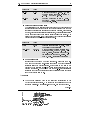
FHI98MD
Computer code for density-functional theory
calculations for poly-atomic systems
✧✧✧
User's Manual
authors of this manual:
P. Kratzer, C. G. Morgan, E. Penev, A. L. Rosa, A. Schindlmayr,
L. G. Wang, T. Zywietz
program version 1.03, August 1999
Contents
1 Introduction
2 Description of the program structure and input les
2.1
2.2
2.3
2.4
2.5
The program structure . . . . . . . . .
The input les inp.mod and start.inp .
The input le inp.ini . . . . . . . . . .
Pseudopotential le(s) . . . . . . . . .
Input les for advanced users . . . . .
2.5.1 The input le constraints.ini .
2.5.2 The input le inp.occ . . . . .
2.6 Runtime control les . . . . . . . . . .
2.7 The output les . . . . . . . . . . . . .
.
.
.
.
.
.
.
.
.
.
.
.
.
.
.
.
.
.
.
.
.
.
.
.
.
.
.
.
.
.
.
.
.
.
.
.
.
.
.
.
.
.
.
.
.
.
.
.
.
.
.
.
.
.
3 Step-by-step description of calculational aspects
3.1
3.2
3.3
3.4
3.5
3.6
How to set up atomic geometries . . . . . .
Choice of the k-point mesh . . . . . . . . .
Total Energy Minimization Schemes . . . .
How to set up a structural relaxation run .
How to set up a continuation run . . . . . .
How to set up a band structure calculation
Bibliography
Index
.
.
.
.
.
.
.
.
.
.
.
.
.
.
.
.
.
.
.
.
.
.
.
.
.
.
.
.
.
.
.
.
.
.
.
.
.
.
.
.
.
.
.
.
.
.
.
.
.
.
.
.
.
.
.
.
.
.
.
.
.
.
.
.
.
.
.
.
.
.
.
.
.
.
.
.
.
.
.
.
.
.
.
.
.
.
.
.
.
.
.
.
.
.
.
.
.
.
.
.
.
.
.
.
.
.
.
.
.
.
.
.
.
.
.
.
.
.
.
.
.
.
.
.
.
.
.
.
.
.
.
.
.
.
.
.
.
.
.
.
.
.
.
.
.
.
.
.
.
.
.
.
.
.
.
.
.
.
.
.
.
.
.
.
.
.
.
.
.
.
.
.
.
.
.
.
.
.
.
.
.
.
.
1
3
3
6
18
23
25
25
25
25
26
27
27
33
38
43
48
49
57
59
iii
Chapter 1
Introduction
Total-energy calculations and molecular dynamics simulations employing densityfunctional theory [1] represent a reliable tool in condensed matter physics, material
science, chemical physics and physical chemistry. A large variety of applications
in systems as dierent as molecules [2, 3], bulk materials [4, 5, 6, 7] and surfaces [8, 9, 10, 11, 12] have proven the power of these methods in analyzing as
well as in predicting equilibrium and non-equilibrium properties. Ab initio molecular dynamics simulations enable the analysis of the atomic motion and allow the
accurate calculation of thermodynamic properties such as the free energy, diusion
constants and melting temperatures of materials.
The package fhi98md described in this paper is especially designed to investigate the material properties of large systems. It is based on an iterative
approach to obtain the electronic ground state. Norm-conserving pseudopotentials [13, 14, 15, 16] in the fully separable form of Kleinman and Bylander [17]
are used to describe the potential of the nuclei and core electrons acting on
the valence electrons. Exchange and correlation are described by either the
local-density approximation [18, 19] or various generalized gradient approximations [20, 21, 22, 23, 24]. The equations of motion of the nuclei are integrated
using standard schemes in molecular dynamics. Optionally, an ecient structure
optimization can be performed by a damped dynamics scheme.
The package fhi98md is based on a previous version fhi96md [25]. The new
version, however, is based on FORTRAN90 and allows dynamic memory allocation. Furthermore, the choice of available gradient-corrected functionals has
been increased. The package consists of the program fhi98md and a start utility fhi98start. The program fhi98md can be used to perform static total energy
calculation or ab initio molecular dynamics simulations. The utility fhi98start
assists in generating the input le required to run fhi98md, thereby ensuring the
lowest possible memory demand for each individual run. Thus no recompilations are
required; a full calculation can be performed by calling the two binary executables
fhi98start and fhi98md in sequence.
This manual consists of two parts. The rst part is a reference list to look up
the function of input parameters, which are described in alphabetical order. The
second part describes typical procedures of how one might use the code. Here
we describe the parameters in their functional context. Also, the way in which the
input parameters control the algorithms used in the code is described in more detail.
Finally, we provide examples of how to use the code to solve a particular physical
problem.
1
Chapter 2
Description of the program
structure and input les
2.1 The program structure
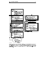
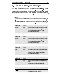
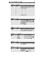
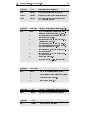
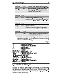
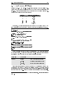
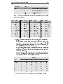
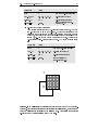
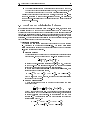
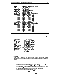
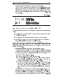
For detailed information about the algorithms used in fhi98md, we refer the interested reader to the article [25]. The structure of the program fhi98md is sketched
in Fig. 2.1. The self-consistent calculation of the electron ground state forms the
main body of the program, which is displayed on the left-hand side of Fig. 2.1.
The movement of the atoms is accomplished in the block \move atoms", which
is sketched on the right hand side of Fig. 2.1. Note that the generation of output
is not explicitly accounted for in the ow chart and we refer to it at the end of this
section.
The rst block in the ow chart is the initialization block, where the program
reads the input les inp.mod, inp.ini and the pseudopotential data. Then the routines calculating form factors, structure factors and phase factors are called and the
initial wave functions are set up either from a restart le or by a few self-consistency
cycles using the mixed basis-set initialization. Having obtained the initial wave function j(0)
i;k i, the program enters the self-consistency loop. First, the electron density
and the contributions to energy, potential and forces are calculated. Note that the
forces are only calculated during MD simulations and structure optimization when
the electrons are suciently close to the Born-Oppenheimer surface.
Within the block \move atoms" the atomic equations of motion (EOMs) are
integrated for one time step in a MD simulation or a structure optimization is
performed, provided the electrons are suciently close to the Born-Oppenheimer
surface, i.e. the forces are converged. The control over the calculation of the forces
is handled by this block. If the nuclei have been moved, i.e. either the atomic
EOMs have been integrated for another time step or one structure optimization
step has been executed, it also recalculates the structure and phase factors and
other quantities that explicitly depend on the positions of the nuclei. Upon the rst
call to the routine fiondyn in this block the restart le fort.20 is read, if provided,
and all necessary steps are taken to restart or initialize the dynamics.
The following two blocks update the wave functions using the damped
Joannopoulos or the Williams-Soler algorithm (see section 3.3) and ortho-normalize
the wave function by a Grahm-Schmidt ortho-normalization. In the last block
within the self-consistency loop the occupation numbers are updated, e.g. for a
metallic system, according to a Fermi distribution, using a mixing scheme between
occupation numbers of subsequent electronic iterations. This block also enables an
interactive control over the remaining numbers of iterations while the program is
3
2.1 The program structure
4
initialization:
header: read inp.mod
init:
read inp.ini and pseudo potentials
calculate structure and form factors
(formf, nlskb, phfac, struct)
set up initial electron density and
wave functions
calculate
rhoofr: electron density n (r)
nlrhkb: non-local contributions
to energy, potential (and forces)
vofrho: local contributions
to energy, potential (and forces)
( )
move atoms (structure optimization or dynamics)
compute
^ KS [n (r)]jn (k)i
dforce: hG + kjH
iterate wave functions jn (k)i
jn (k)i ! jn (k)i
repeat for all states
perform
graham: Grahm-Schmidt orthonormalisation
j (k)i,. . . ,jn (k)i
( )
( )
( )
( )
( +1)
( +1)
1
call
: for structure optimization
: molecular dynamics
both routines monitor the error of the forces and
move the ions after convergence.
fionsc
fiondyn
no have atoms been moved ?
S
S
yes
! +1
TT
recalculate
struct,
structure and phase factors
phfac:
calculate
nlrhkb: non-local contributions
to energy, potential (and forces)
vofrho: ewald sum and local contributions
to energy, potential (and forces)
( +1)
repeat for all k-points
calculate (e.g. for metals):
fermi:
occupation according to fermi
distribution
validate
iteration parameters (c.f. les delt,
stople and stopprogram).
T
terminate
on convergence
or
if number of iterations or
cpu-time is exceeded
terminate
Figure 2.1: Flow chart of the program fhi98md. Output is generated at the end of
each self-consistency cycle and by the routines fiondyn, fionsc, fermi, init and vofrho.
Restart les are written by the routine fiondyn and by a call of routine o wave in the
main program.
2.1 The program structure
5
running. These parameters are updated from the les stople (remaining number of
electronic iterations) and stopprogram (remaining number of structure optimization
steps). If these les are empty the parameters are not changed. Finally, the convergence criteria are checked. The program terminates when convergence is achieved
or when the preset number of iterations or the allowed CPU-time is exceeded.
Output is generated at the last block of the self-consistency loop and by the
routines fiondyn, fionsc, fermi and vofrho. The routines fiondyn and o wave
generate restart les for MD simulations and total-energy calculations.
In the mixed-basis-set initialization, the self-consistency loop closely follows the
organization of that discussed above. First of all the initial electron density is
obtained either from a superposition of contracted atomic pseudo densities or from
an electron density of a previous calculation (le fort.72). The local contributions
to the potential and the energy are calculated by the routine vofrho. The localized
orbitals to construct the mixed-basis-set are set up by the routine project. The
non-local contributions to the potential and the energy in the localized basis set
are calculated by the routine nlrhkb b. In the second step the Hamiltonian is
constructed with the help of routine dforce b. The Hamiltonian is diagonalized by
standard diagonalization routines. The new electron density is calculated (routine
rho psi). Finally the new electron density is mixed with the old density by a
Broyden mixing (routine broyd).
2.2 The input les inp.mod and start.inp
6
2.2 The input les inp.mod and start.inp
Two input les are required as input for the start utility fhi98start. The le
inp.mod contains the control parameters for the run. The le start.inp describes
the geometry of the super cell and the conguration of the nuclei. It also contains
information that is relevant for the MD simulation or the structure optimization,
and the calculation of the electron ground state.
❏
inp.mod
The le inp.mod contains mainly the control parameters for the runs, like
e.g. the time steps for the electronic and atomic minimization schemes, the
convergence criteria and maximum number of steps etc. In the following, the
parameters are explained in alphabetical order.
Parameter
ampre
Type
real
Parameter
amprp
Type
real
Parameter
delt
Type
real
Parameter
delt2
Type
real
Parameter
delt ion
Type
real
an amplitude of a random perturbation is
added to the wave function, but only if
the parameter trane is set to .true.
see also parameter trane
an amplitude of a random perturbation is
added to the ionic positions, but only if
the parameter trane is set to .true.
see also parameter trane
step length of the electronic iteration: this
value has to be individually optimized in
order to obtain optimal convergence
see also parameter delt2
second step length of the electronic iteration
connected to parameter eps chg dlt
(only relevant for MD simulations)
time step for the integration of the ionic
equations of motion (in a.u.)
2.2 The input les inp.mod and start.inp
Parameter
Type
epsekinc
real
epsel
real
epsfor
real
criteria to end self consistent cycle (in a.u.):
stop if the average change of wave functions for
the last three iterations is less than epsekinc and
if the variation of the total energy is less than epsel
for the last three iterations and
if the forces on ions are smaller than epsfor; this
parameter is only active if tfor and tford is .true.
Parameter
eps chg dlt
Type
real
Parameter
force eps
Type
force eps(1)
real
force eps(2)
real
Parameter
gamma
Value
real
gamma2
real
if the total energy varies less than
eps chg dlt, the parameters delt and
gamma are replaced by delt2 and gamma2
connected to parameter delt, delt2,
gamma, gamma2
convergence criteria for local and total
forces:
maximum allowed relative variation in local forces before, if tfor is .true., executing a geometry optimization step or, if
tdyn is .true., calculating total forces
maximum allowed relative variation in total forces before moving ions (if tdyn is
.true.)
connected to parameter tfor and tdyn
damping parameter for the second order electronic minimization scheme (only
used if i edyn is 2)
second damping parameter: refer to
eps chg delt
connected to i edyn and eps chg delt
7
2.2 The input les inp.mod and start.inp
Parameter
i edyn
Value
scheme to iterate the wave functions:
steepest descent
Wiliams-Soler algorithm (rst order)
damped Joannopoulos algorithm (second
order)
0
1
2
Parameter
i xc
Value
exchange-correlation functional:
LDA
(Ceperley/Alder
[18],
Perdew/Zunger [19])
Beckex/Perdewc (BP) [20, 21]
Perdew/Wangxc (PW91) [22]
Beckex; Lee/Yang/Par (BLYP) [23]
Perdew/Burke/Ernzerhofxc (PBE) [24]
0
1
2
3
4
Parameter
idyn
Value
0
1
2
Parameter
initbasis
(only relevant for MD simulations)
scheme for solving the ionic equation of
motion only active if tdyn is .true.:
predictor corrector
predictor
Verlet-algorithm
connected to nOrder and tdyn
Value
1
2
3
type of basis set used in the initialization (if nbeg
is set to -1):
plane-wave basis set
LCAO basis set
mixed basis set (LCAO and plane waves)
connected to ecuti and tinit basis in le start.inp
Parameter Type
iprint
integer number of electronic iterations between a detailed
output of (i ) energies and eigenvalues in le fort.6
and (ii ) restart les fort.70 (wave functions) and
(iii ) fort.72 (electron density)
8
2.2 The input les inp.mod and start.inp
Parameter
max no force
Type
integer
maximum number of electronic iterations
for which no local forces shall be calculated per ionic step
Parameter
Type
mesh accuracy real degree to which the sampling theorem shall be
satised. The sampling theorem implies that the
size of the Fourier mesh, nrx(1)nrx(2)nrx(3),
which determines the accuracy of the
p charge density, should obey nrx(1) 2 jja1 jj Ecut; likewise
for nrx(2) and nrx(3). Using smaller values for nrx
means
the highest G-vectors in n(r) =
P P skipping
P
~
w
~
k
k i G;G fi;k ci;G~ +k ci;G+kei(G;G)r and
results in a faster performance. However, the
applicability of the grid should then be carefully
checked. For systems with strongly localized orbitals, in particular, this may be an unacceptable
approximation.
Parameter
nbeg
Value
-1
-2
set-up of the initial wavefunction
the initial wave function is obtained by diagonalization of the Hamiltonian matrix in the basis set
as specied by tinit basis
the initial wavefunction is read in from le fort.70
connected to tinit basis
Parameter
nomore
Type
integer
nomore init
integer
maximum number of electronic steps if
tfor and tdyn are .false. or maximum
number of atomic moves if tfor and tdyn
are .true.
maximum number of steps in the initialization if nbeg is -1
see also nbeg and init basis
9
2.2 The input les inp.mod and start.inp
Parameter
nOrder
Type/Value
integer
0
1
2
3
Parameter
nstepe
Type
integer
Parameter
pt store
Type
real
Parameter
t postc
order of the scheme for solving the ionic
equation of motion if idyn is set to 0 or 1:
predictor corrector
1
2
2
3
3
4
4
5
connected to idyn
if tfor or tdyn is .true.: maximum number of electronic iterations allowed to converge forces, the program terminates after
nstepe iterations
see also force eps
fraction of wavefunctions for which a
second transformation to real space is
avoided (currently not implemented)
Type/Value
logical
.true.
.false.
Parameter
tdipol
Type
logical
Parameter
tdyn
Type
logical
10
post LDA functional:
post LDA with functional i xc
start with functional i xc
if set to .true. the surface dipol correction is calculated
if set to .true. a molecular dynamics
simulation is performed, tfor must be set
to .false.
connected to force eps and tford
2.2 The input les inp.mod and start.inp
Parameter
tfor
Type
logical
Parameter
timequeue
Type
integer
Parameter
trane
Type
logical
Parameter
tranp
Value
logical
Parameter
tsdp
Type/Value
logical
.true.
.false.
❏
11
if set to .true. ionic positions are relaxed, tdyn must be set to .false.
connected to force eps, epsfor and tford
maximum CPU time in seconds: the program writes output and restart les before
the limit is exceeded and the program is
terminated automatically
if set to .true. the initial wave functions
are perturbed by the value trane
connected to ampre
if set to .true. the ions which are allowed
to move are perturbed by amprp Bohr
connected to amprp
scheme for structural optimization:
modied steepest descent scheme
damped dynamics scheme
Example The sample input le inp.mod below sets up a typical bulk calculation for metallic Ga. The parameters are given in the order required
by the fhi98md program. The corresponding start.inp le is given in
the section below.
inp.mod
-1 100 1000000
: nbeg
iprint timequeue
100 2
: nomore nomore_init
6.0 0.2
: delt gamma
4.0 0.2 0.0001
: delt2 gamma2 eps_chg_dlt
400 2
: delt_ion nOrder
0.0 1.0
: pfft_store mesh_accuracy
2 2
: idyn i_edyn
0 .false.
: i_xc t_postc
.F. 0.001 .F. 0.002
: trane ampre tranp amprp
.false. .false. .false. 1800 : tfor tdyn tsdp nstepe
.false.
: tdipol
0.0001 0.0005 0.2
: epsel epsfor epsekinc
0.001 0.001 3
: force_eps(1) force_eps(2) max_no_force
3
: init_basis
2.2 The input les inp.mod and start.inp
❏
12
start.inp
The le start.inp contains all structural informations: the geometry of
the supercell and e.g. the positions of the nuclei. All parameters in the
start.inp necessary for the fhi98md program are given in alphabetical
order below.
Parameter
atom
Type
character*10
Parameter
celldm(1..6)
Type
real
Parameter
coordwave
Type
logical
Parameter
ecut
Type
real
Parameter
ecuti
Value
real
name of the pseudopotential supplied,
necessary for each species
lattice parameters of the supercell;
celldm(1) gives typically the lattice constant in bohr
if set to .true. and nrho is set to 2 the
ionic positions are read in from the le
fort.70
connected to nrho
plane wave energy-cuto in Rydberg; the
cuto depends on the pseudopotentials
and has to be individually checked for every system
plane wave energy-cuto for the initialization if plane waves or a mixed basis are
chosen by the parameter init basis in the
le inp.mod
connected to init basis
2.2 The input les inp.mod and start.inp
Parameter
ekt
Type
real
13
temperature of the articial Fermi smearing of the electrons in eV if tmetal =
.true.; this parameter has to be optimized for each system in order to obtain optimal convergence. For instance, in
case of semiconductor systems smallness
of this parameter would ensure that the
semiconducting character is unaected.
Commonly used values lie in the range
0.01{0.10 eV
connected to tmetal
Parameter Type/Value
ibrav
integer
cell type: the cell types are specied in
the routine latgen and can be specied
individually; the most common cell types
are available
0
structure is kept as supplied in the le start.inp
1
simple cubic lattice
2
fcc-lattice
3
bcc-lattice
8
orthorhombic
connected to celldm
see also: How to set up atomic geometries
Parameter
ion damp
Parameter
ion fac
Type
real
damping parameter 2 [0; 1]; only active if tfor is
set to .true. and tsdp is set to .false.
connected to tfor and tsdp
see also: How to set up a structural relaxation run
Type
real
mass parameter if tfor is set to .true.; if
tdyn is set to .true. ion fac species the
ionic mass in a.u.
connected to tdyn and tfor
2.2 The input les inp.mod and start.inp
Parameter
i facs(1..3)
Type
integer
Parameter
lmax
Type
integer
Parameter
l loc
Type
integer
Parameter
na
Type
integer
Parameter
nel exc
Type
real
Parameter
nempty
Parameter
n rescale
Parameter
nkpt
k-point folding factors: 1 1 1 corresponds to no folding
connected to tfor and tsdp
see also: Choice of the k-point mesh
highest angular momentum of the pseudopotential (1 ! s, 2 ! p, 3 ! d)
connected to l loc
angular momentum of the local pseudo
potential (l loc lmax)
connected to lmax
number of atoms of speciesis; has to be
specied for each element
number of excess electrons (required for
a calculation with a charged supercell for
bulk defect calculations)
Type
integer
Type
integer
14
number of empty states
only for MD simulations (if tdyn is .true.)
number of ionic moves before velocities
are rescaled; only active if nthm is 1
connected to nthm
Type
integer
number of k-points
2.2 The input les inp.mod and start.inp
Parameter
npes
minpes
ngrpx
Type
integer
integer
integer
only relevant for parallel code
number of processor elements (PE's)
minimal number of PE's (currently inactive)
number of PE's in a group performing the
FFT (currently inactive)
Parameter
npos
Type/Value
integer
only for MD simulations (if tdyn is .true.)
set up of initial ionic positions and velocities; only active if tdyn is set to .true.
coordinates tau0 and velocities vau0 are
read in from le start.inp
coordinates are read in from le fort.70,
velocities from le fort.20
coordinates are read in from le fort.70,
the velocities are set according to the initital temperature set by T init
set according to 1, but the total momentum is set to zero
set according to 3, but the total momentum is set to zero
restart from le fort.20
connected to tdyn, T init, tau0 and vau0
1
2
3
4
5
6
Parameter
nrho
Type/Value
integer
1
2
3
Parameter
nseed
Parameter
nsp
Type
integer
Type
integer
set up of the initial electron density
superposition of atomic electron densities
constructed from le fort.70
read in from le fort.72
only for MD simulations (if tdyn is .true.)
seed used to generate initial velocities
number of atomic species
15
2.2 The input les inp.mod and start.inp
Parameter
nthm
Type/Value
integer
0
1
2
Parameter
pgind
Type/Value
integer
0
1
..
.
only for MD simulations (if tdyn is .true.)
simulation ensemble for the ions; only active if tdyn is set to .true.
micro-canonical ensemble
micro-canonical ensemble, but the velocities are rescaled
canonical ensemble (Nose-Hoover)
connected to n rescale and Q
point group index:
automatic (symmetries and center)
no symmetries assumed
see also parameter ibrav and latgen.f
connected to ibrav
see also: How to set up atomic geometries
Parameter
Q
Type
real > 0
Parameter
t init basis
Type
3 logical
only for MD simulations (if tdyn is .true.)
if nthm= 2: mass of thermostat in a.u.
if set to .true.: include s; p; and d LCAO
orbitals in the initialization; only active if
init basis is 2 or 3
connected to init basis
Parameter
T init
Type
real
only for MD simulations (if tdyn is .true.)
temperature of initial velocities in K; only
active if npos is either 3 or 5
connected to npos
Parameter
T ion
Type
real
only for MD simulations (if tdyn is .true.)
ionic temperature in K; only active if
nthm is either 1 or 2
connected to nthm
16
2.2 The input les inp.mod and start.inp
Parameter
t kpoint rel
Value
.false.
.true.
Parameter
tau0(1..3)
Type
real
Parameter
tband
Type
logical
Parameter
tdegen
Type
logical
Parameter
tmetal
Type/Value
logical
.true.
.false.
Parameter
tmold
Parameter
tpsmesh
Type
logical
k-points are given in Cartesian coordinates in units 2=alat
frame of reference for k-points is spanned
by the reciprocal lattice vectors, i.e. k =
k1 b1 + k2 b2 + k3 b3
ionic coordinates (units depend on ibrav),
ag whether atoms may move given by
tford
connected to tford
if set to .true. the k-point set is not reduced by fhi98start utility; the electron
density is not recalculated after the initialization
if set to .true. the initial occupation
numbers are read in from le inp.occ (kept
xed for the run)
occupation of the electronic states:
Fermi distribution (see also ekt)
step-like distribution
connected to ekt
if set to .false. only the initialization is
performed
Type/Value
logical
.true.
.false.
17
form of the pseudopotential
tabulated on logarithmic mesh
set up from parameterized form
2.3 The input le inp.ini
Parameter
vau0(1..3)
18
Type
real
Parameter
wkpt
Type
real
Parameter
xk(1..3)
Type
real
only for MD simulations (if tdyn is .true.)
ionic velocities in a.u.; only active if tdyn
is set to .true. and npos is either 1 or 4
connected to tdyn and npos
weights of the k-points given by xk(1..3)
connected to xk(1..3), nkpt, i facs and t kpoint rel
k-point coordinates
connected to wkpt, nkpt, i facs and t kpoint rel
Parameter
zv
❏
Type
real
valence charge of the pseudopotential; to
be supplied for each element
Example The sample input le start.inp below sets up a typical bulk
calculation for metallic Ga. The parameters are given in the order required by the fhi98md program.
start.inp
1
1
1
1
0
2
2 0
10.682 0.0 0.0 0 0 0
40
0.5 0.5 0.5 0.025
1 1 1
.false.
8.0 4.0
0.005 .true. .false.
.true. .true. 1
5 2 1234
873.0 1400.0 1e8 1
.true. .true.
1 3 'Gallium'
1.0 3.0 0.7 3 3
.t. .t. .f.
0.0 0.0 0.0
.f.
:
:
:
:
:
:
:
:
:
:
:
:
:
:
:
:
:
:
:
:
:
:
npes, number of processors
npesmin, number of minimal processors
npespg, number of processors per group
number of species
excess electrons
number of empty states
ibrav pgind
celldm(6)
number of k-points
k-point coordinates, weight
fold parameter
k-point coordinates relative or absolute?
Ecut [Ry], Ecuti [Ry]
ekt tmetal tdegen
tmold tband nrho
npos nthm nseed
T_ion T_init Q nfi_rescale
tpsmesh coordwave
number of atoms, zv, name
gauss radius, mass, damping,l_max,l_loc
t_init_basis
tau0 tford
2.3 The input le inp.ini
The input le inp.ini is usually generated automatically by the start utility
fhi98start from the les inp.mod, start.inp and constraints.ini. However, the program fhi98md also runs individually without the help of the start utility. This
requires the user to provide the le inp.ini in addition to inp.mod, the pseudopotentials and possible restart le(s).
2.3 The input le inp.ini
❏
19
inp.ini
The le inp.ini contains processed data from start.inp plus a copy of constraints.ini. All new quantities are described below in alphabetical order,
while unchanged parameters taken from either start.inp or constraints.ini are
not listed again. We refer instead to the detailed information given earlier.
Parameter
a1(1..3)
a2(1..3)
a3(1..3)
Type
3 real
3 real
3 real
Parameter
alat
Type
real
Parameter
b1(1..3)
b2(1..3)
b3(1..3)
Type
3 real
3 real
3 real
Parameter
ineq pos(1..3)
Type
3 integer
Parameter
max basis n
Type
integer
Parameter
mmaxx
Type
integer
Parameter
n t store
Type/Value
integer (= 1)
lattice vectors in a.u.
lattice constant in a.u.
reciprocal lattice vectors in a.u.
if t coord auto = :true:: number of mesh
points along the corresponding lattice vector of the super cell, the mesh must contain the origin (0; 0; 0) of the super cell
connected to t coord auto(1..3)
max basis n = max(nx ; nx basis )
connected to nx and nx basis
maximum size of pseudo-potential grid
[option currently not implemented]
2.3 The input le inp.ini
20
Parameter
nax
Type
integer
maximum number of atoms per species
Parameter
nel
Type
real
number of electrons
Parameter
ngwix
Type
integer
Parameter
ngwx
Type
integer
Parameter
nlmax
Type
integer
Parameter
nlmax init
Type
integer
Parameter
nnrx
Type
integer
Parameter
nrot
Type
integer
maximum number of plane waves during
the initial diagonalization; should obey
ngwix 16 ;2 omega ecuti 3=2
connected to omega and ecuti
maximum number of plane waves used to
represent the wave functions, should obey
ngwx 16 ;2 omega ecut 3=2
connected to omega and ecut
nlmax = max(l max 2 ; 2 l loc + 1)
connected to l max and l loc
maximum number of atomic orbitals per
atom in the initialization
nnrx = (nrx (1 ) + 1) nrx (2 ) nrx (3 )
connected to nrx(1..3)
number of point symmetries
connected to s(3,3)
2.3 The input le inp.ini
21
Parameter
nrx(1..3)
Type
integer
Parameter
nschltz
Value
0
1
Parameter
nsx
Type
integer
Parameter
nx
Type
integer
Parameter
nx basis
Type
integer
Parameter
nx init
Type
integer
Parameter
omega
Type
real
Parameter
s(3,3)
Type
real
dimensions of the Fourier mesh, should
obey nrx (1 ) 2;1 jja1 jj ecut 1=2 , etc.
connected to a(1..3) and ecut
control ag for ecient storage allocation,
should be set to zero unless i edyn = 2
damped Joannopoulos algorithm disabled
all iteration schemes enabled
connected to i edyn in inp.mod
maximum number of atomic species
maximum number of electronic states per
k-point
maximum number of atomic orbitals in
the initialization
nx init = ngwix + nx basis
connected to ngwix and nx basis
super cell volume in a.u.
connected to a1(1..3), a2(1..3), a3(1..3)
33 point-symmetry matrices in units of
the lattice vectors
connected to nrot
2.3 The input le inp.ini
Parameter
t coord auto(1..3)
❏
22
Type
logical
if tford = :false:: enable more ecient
treatment of xed ions on a mesh commensurate with the super cell
connected to tford and ineq pos(1..3)
Example
The input le inp.ini below was generated from the sample les start.inp and
constraints.ini for metallic Ga given earlier. The parameters are arranged in
the order expected by the main program fhi98md.
inp.ini
1
4
11
739
5912
: nsx,nax,nx,ngwx+1,ngwx*8+8
102
118
24
24
24
1 : ngwix,nx_init,nrx(1),nrx(2),nrx(3),nschltz
16
16
4
: nx_basis,max_basis_n,nlmax_init
14400
39
4
570
1
: nnrx,nkpt,nlmax,mmaxx,n_fft_store
1
1
1
: minpes, ngrpx, nrpes
12
0
: ibrav, pgind
12.0000
T
0.10000
F
: nel,tmetal,ekt,tdegen
20.00000
5.00000
: ecut,ecuti
T
F
1
: tmold,tband,nrho
5
2 1234
: npos, nthm, nseed
873.00 1400.00 0.1000E+09
1
: T_ion, T_init, Q, nfi_rescale
1
T
T
: nsp,tpsmesh,coordwave
39
: nkpt
0.1000000
0.0000000
0.1182033
0.0160000 :xk(1-3),wkpt
...
...
...
...
8.25000000
0.00000000
0.00000000
: lattice vector a1
0.00000000
4.11262491
6.97950013
: lattice vector a2
0.00000000
-4.11262491
6.97950013
: lattice vector a3
1.00000000
0.00000000
0.00000000
: rec. lattice vector b1
0.00000000
1.00300905
0.59101654
: rec. lattice vector b2
0.00000000
-1.00300905
0.59101654
: rec. lattice vector b3
8.2500000
473.61709094
: alat,omega
'Gallium
'
4
3.00000 69.72000 : name,number,valence charge, ion_fac
0.70000 1.00000 3 3
: ion_damp,rgauss,l_max,l_loc
T
T
F
: t_init_basis s,p,d
0.651750030
0.000000000
2.135727000
F
F
F
T
-0.651750030
0.000000000
-2.135727000
F
F
F
T
4.776750030
0.000000000
4.843773130
F
F
F
T
3.473249970
0.000000000
9.115227130
F
F
F
T
0
0
0
: ineq_pos
4
: nrot = number of symmetries
1--------1
0
0
0
1
0
0
0
1
2--------1
0
0
0
0
1
0
1
0
3---------1
0
0
0
0 -1
0 -1
0
4---------1
0
0
0 -1
0
0
0 -1
0
0
2.4 Pseudopotential le(s)
23
2.4 Pseudopotential le(s)
Besides the inp.mod and start.inp/inp.ini les considered so far the fhi98md requires supply of pseudopotentials for each of the nsp atomic species listed in
start.inp. Pseudopotential le(s) must be provided in the working directory according to the following naming convention:
species #
pseudopotential lename
1
!
fort.11
2
!
fort.12
..
..
..
.
.
.
nsp
!
fort.1nsp
In practice, the pseudopotential data are copied to the working space by the
same shell script (batch le under Windows) which runs the fhi98md program.
#! /bin/csh -xvf
....
############## set directories ######################
set PSEUDO
set WORK
.....
=
=
[pseudopotentials directory]
[working directory]
########### change to the working space #############
cd $WORK
#### move pseudopotentials to the working space
####
cp $PSEUDO/ga:lda:ham.cpi fort.11
cp $PSEUDO/as:lda:ham.cpi fort.12
.....
######################################################
#
run fhi98md
#
######################################################
./fhi98md
.....
Pseudopotentials are read in during the initialization when control is delivered
to the init routine1 . The tpsmesh parameter in start.inp allows the user to instruct
the fhi98md about the format of the pseudopotential data le(s):
Parameter
tpsmesh
Type/Value
logical
.true.
.false.
form of the pseudopotential
tabulated on logarithmic mesh
set up from parametrized form
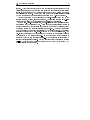
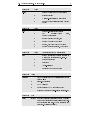
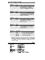
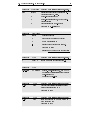
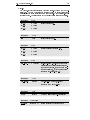
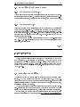
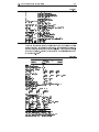
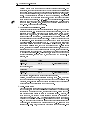
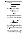
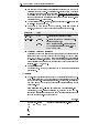
Ionic pseudopotentials in the format accepted by the fhi98md program can
be generated and tested by means of the fhi98pp package. The latter provides
the psgen tool which produces as chief output a pseudopotential data le name.cpi
formated as shown in Fig. 2.2 (for more details the user is referred to the article [26]).
1 The current version of init supports up to 6 pseudopotential
nsp > 6.
les. Customize this routine for
2.4 Pseudopotential le(s)
1
Z ion lmax + 1
2
.
.
.
11
12
24
[unused]
mmax
amesh
block for l = 0
13
.
.
.
ps
ps
m rm ups
l (l ; rm ) Vl (rm )
mmax +11
eld
Z ion
lmax + 1
mmax
amesh
m
rm
ups
l
Vlps
description
number of valence electrons
number of pseudopot. components
number of radial mesh
points
mesh increment rm+1 =rm
mesh index
radial coordinate (in bohr)
radial pseudo wavefunction
ionic pseudopotential (in
hartree)
..
.
block for l = lmax
[like for l = 0]
.
.
.
partial core density block
appears only if core-valence
exchange-correlation applies;
see Ref. [26]
Figure 2.2: Format of the pseudopotential le name
.cpi
as generated by the psgen tool.
When setting up the start.inp le one should ensure that the values of the zv
and lmax parameters match those of the Zion and lmax +1 elds, respectively, in the
pseudopotential les for each species. The fhi98md program stops if zv 6= Zion or if
not enough angular momentum components have been provided, i.e. lmax +1 < lmax
Parameter
lmax
Type
integer
l loc
integer
highest angular momentum of the pseudopotential (1 ! s, 2 ! p, 3 ! d)
angular momentum of the local pseudo
potential (l loc lmax)
Special care should be paid also to the l loc parameter(s) in le start.inp: it
must be set to the same value used in generating the pseudopotential. If for any
reason the user would like to change l loc, then a new pseudopotential has to be
constructed according to the new l loc value.
Sometimes an explicit account of the core-valence nonlinearity of the exchangecorrelation functional is required, for instance in studies involving alkali metal
atoms [26]. In this case the psgen tool appends at the end of the name.cpi le
a data block containing the partial core density, Fig. 2.2. The fhi98md program
automatically recognizes the use of such a pseudopotential and the proper information record is written to fort.6 during the initialization.
Note also that pseudopotentials should be generated and used within the same
exchange-correlation scheme.
2.5 Input les for advanced users
25
2.5 Input les for advanced users
2.5.1 The input le constraints.ini
This le allows the user to specify constraints for the atomic motion when a structural relaxation run is performed. For using this feature, consult the section 3.4. If
no constraints are required, this les contains two lines, both with a 0 (zero) in it.
2.5.2 The input le inp.occ
This input le allows for a calculation where the occupation of the eigenstates
of the system is user-specied. This feature is mostly used in conjunction with
calculations of atoms and molecules. To activate this feature, set tdegen to .true.
in the input le start.inp. The le inp.occ should consist of one line, with the
occupation numbers (real numbers between 0.0 and 2.0) listed in the order of
ascending energy eigenvalues.
A typical le that would impose spherical symmetry on a three-valent single
atom (e.g. Ga, In etc.) regardless of the symmetry of the unit cell employed in the
calculation, is shown below:
inp.occ
2.0 0.333333 0.333333 0.333333 0.0
Thus, the s subshell is completely occupied by 2 electrons and to each of the
three p orbitals (px;y;z ) is assigned 1/3 occupancy. Note, however, that in this
particular case the nempty variable in start.inp should be set to 2 and not to 1
as one could deduce from inp.occ. This is easy to realize having in mind that the
maximum number nx of electronic states per k-point is dened as nx = nempty +
( nel +1.0)/2.0.
2.6 Runtime control les
The les stopprogram and stople allow to control the program execution during
runtime. They both consist of one line with one integer number. The le stopprogram can be used to stop the program execution deliberately. If the number of
electronic iterations already performed exceeds the number given in stopprogram,
the fhi98md program terminates.
The le stople allows to reset the variable nomore while the program is running. Please notice that the meaning of nomore depends on the mode in which the
program is run (electronic structure only, or relaxation/molecular dynamics run).
In both cases, the program only ends after all output les are written, thus
enabling a continuation of the run (see section How to set up a continuation run).
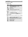
2.7 The output les
26
2.7 The output les
❏
Main output les
lename
energy
fort.1
fort.6
report.txt
status.txt
❏
Output les for data analysis using the EZWAVE graphical user
interface
fort.80
rhoz
❏
contents
number of iterations, total energy in Hartree (at nite electronic temperature !), Harris energy in Hartree
atomic relaxations and forces
general output
summary of the run
current state of the calculation, error messages
for visualization of the potentials
charge density along the the z-axis (i.e. at x; y = 0)
Binary output les
(used for restarting the program or for analysis of the run with utility programs)
fort.21
fort.71
fort.72
fort.73
fort.74
when performing molecular dynamics: positions and velocities of the atoms along the trajectory
complete restart information, including all wavefunctions
electronic charge density
total eective potential
electrostatic potential
Chapter 3
Step-by-step description of
calculational aspects
3.1 How to set up atomic geometries
Before an electronic structure calculation can be performed, it is necessary to specify
a starting geometry for the atomic structure of the system we want to study. If this
geometry is invariant under certain discrete crystallographic symmetry operations,
the computational load can be reduced considerably by exploiting these symmetries.
Therefore it is recommended to analyze the symmetry of the atomic geometry before
starting the calculation, and to choose the unit cell in such a way that a maximum
number of symmetries is met. The fhi98md code is distributed together with
the fhi98start utility which helps to search for relevant symmetries and to set up
crystals and slabs from some standard crystallographic symmetry classes.
Under UNIX environment, for example, the fhi98start utility is usually
invoked by the same shell-script that runs fhi98md (below a protocol of the
fhi98start run is saved in the le start.out):
#! /bin/csh -xvf
.....
set FHI98MD = ~/fhi98md
.....
cp ${FHI98MD}/fhimd/fhi98md .
cp ${FHI98MD}/start/fhi98start .
.....
######################################################
# run fhi98start program and build up inp.ini
#
# - in principle one could create inp.ini by hand,
#
#
but fhi98start gives a consistent and optimized #
#
input for fhi98md
#
######################################################
./fhi98start | tee start.out
######################################################
#
run fhi98md
#
######################################################
./fhi98md
.....
❏
Basic input parameters
All input information about crystal structure is produced by the fhi98start
utility according to the values of the following parameters specied in the le
start.inp:
27
3.1 How to set up atomic geometries
❏
Parameter
ibrav
pgind
celldm(1..6)
Type
integer
integer
6 real
tau0(1..3)
3 real
28
Bravais lattice
point-group index
lattice parameters of the super
cell (depends on ibrav)
coordinates of the nuclei (units
depend on ibrav)
Setting up parameter values
First the user species whether he/she wants to set up the crystallographic vectors (a1 ; a2 ; a3 ) spanning the unit cell directly (ibrav = 0 in
start.inp), or prefers to select the type of the super cell to be used in the
calculation from a pre-dened list (ibrav > 0).
In the rst case, the crystallographic vectors (a1 ; a2 ; a3 ) should be specied in three input lines at the end of start.inp. In the latter case, for
(ibrav > 0), the fhi98start utility calls the latgen routine (latgen.f)
that sets up the crystallographic vectors (a1 ; a2 ; a3 ). In both cases, their
reciprocal counterparts (b1 ; b2 ; b3 ) are calculated. The following lattice
symmetries are implemented:
Parameter
ibrav
Value
0
1
2
3
4
8
10
12
user-supplied cell
simple cubic (sc)
face centered cubic (fcc)
body centered cubic (bcc)
hexagonal: Zn-bulk (hcp, A3 structures)
orthorhombic
rhombohedral (A7 structures)
base centered orthorhombic (A11, A20 structures)
Specify how fhi98start should determine point-group symmetries|
parameter pgind in start.inp.
With pgind = 0 an automatic search for the point group symmetries and
the symmetry center is performed. This is the preferred setting. Notice however that all input coordinates may get shifted if this enables to
enhance the number of symmetries. In successive restart runs, if there
is the risk that the number of point-group symmetries (variable nrot)
may change unwantedly between the runs, set pgind = 1 in order to
avoid conicts. pgind values in the range 2{32 could be used, for instance, for some specic purposes in structural relaxation runs (see also
How to set up structural relaxation run).
3.1 How to set up atomic geometries
Parameter
pgind
29
Value
automatic search for symmetries
no symmetries assumed 1 (C1 )
point-group index
0
1
2{32
pgind 1 denes the crystallographic point group as follows (for more details
consult pgsym routine):
pgind
1
2
3
4
5
6
7
8
Group
1 (C1 )
1 (Ci )
2 (C2 )
m (Cs )
2=m (C2h )
3 (C3 )
3 (S6 )
32 (D3 )
pgind
9
10
11
12
13
14
15
16
Group
3m (C3v )
3m (D3d )
4 (C4 )
4 (S4 )
4=m (C4h )
422 (D4 )
4mm (C4v )
42m (D2d )
pgind
17
18
19
20
21
22
23
24
Group
4=mmm (D4h )
6 (C6 )
6 (C3h )
6=m (C6h )
622 (D6 )
6mm (C6v )
62m (D3h )
6=mmm (D6h )
pgind
25
26
27
28
29
30
31
32
Group
222 (D2 )
2mm (C2v )
mmm (D2h )
23 (T )
m3 (Th )
432 (O )
43m (Td )
m3m (Oh )
Dene the lattice parameters of the super cell|parameter celldm in
start.inp
The meaning of each celldm component depends on ibrav. Usually celldm(1) contains the lattice constant a in bohr. For hexagonal and rhombohedral super cells, ibrav = 4 and 10 respectively, the
c=a ja3 j=ja1 j ratio is specied in celldm(2).
♦ When dening systems having A7 structure (the common crystal phase
of As, Sb and Bi, ibrav = 10), the positions of the two atoms in the basis
are given by u(0; 0; c); where the dimensionless parameter u should be
provided in celldm(3).
♦ In certain cases (ibrav = 4; 10; 12) the input format allows also for
n1 n2 n3 scaling of the super cell. The three scaling factors ni ;
i = 1; 2; 3; are specied in celldm(4..6) respectively:
♦
ibrav
1,2,3
4
8
10
12
1
a
a
a
a
a
2
{
celldm(i)
3
4
{
{
{
n1
c
{
c=a
b
c=a
u
{
{
n1
n1
5
{
6
{
n2
n3
{
{
n2
n2
n3
n3
Specify coordinates of the nuclei|parameter tau0(1..3) in start.inp
3.1 How to set up atomic geometries
30
The value of ibrav determines the units in which tau0(1..3) are to be
given:
units [tau0(1..3)]
alat := celldm (1 )
atomic units, aB = 0:529177 A
ibrav
1,2
3,4,8,10,12
For ibrav = 4; 10 and 12, positions of the nuclei are solely determined
by celldm; therefore the supplied values of tau0(1..3) are not signicant.
Thus, the following fragment from start.inp is an allowed input:
.....
10 0
7.1 2.67 0.227
.....
2 5 'Arsenic'
1.0 74.92 0.7
.t. .t. .f.
0.0 0.0 0.0
0.0 0.0 0.0
❏
: ibrav pgind
1 1 1 : celldm
3 3
.f.
.f.
:
:
:
:
:
number of atoms, zv, name
gauss radius, mass, damping,l_max,l_loc
t_init_basis
tau0 tford
tau0 tford
Other features
Cluster calculations
To set up a cluster calculation with fhi98md you need to follow the
same steps described above. It is important, however, that you take
a suciently large super cell in order to avoid coupling between the
periodic images of the nite system. The common practice is to place
the cluster in a cubic (ibrav = 1) or orthorhombic (ibrav = 8) unit
cell whose size should be tested to satisfy the above condition (see also
Choice of the k-point mesh).
Slab calculations
The ibrav value in this case should be chosen to reect the symmetry of the surface unit cell employed in the calculation. Coordinates
of the nuclei are specied as described above. The size of the super cell in the direction perpendicular to the surface should ensure a
large enough vacuum region between the periodic slab images (see also
Choice of the k-point mesh).
❏
Examples
The A7 crystal structure of As1
A sample start.inp le to set up bulk calculation for the A7 structure
(ibrav = 10) of As with lattice parameters alat = 7:1 bohr, c=alat = 2:67
and u = 0:227 as specied in celldm(1..3). No scaling of the super cell
will be performed|celldm (4 ::6 ) = (1:0; 1:0; 1:0): In order to switch on
the automatic search for symmetries pgind has been set to 0.
1 see for example R. J. Needs, R. Martin, and O. H. Nielsen, Phys. Rev. B 33, 3778 (1986).
3.1 How to set up atomic geometries
31
start.inp
1
1
1
1
0
5
10 0
7.1 2.67 0.227 1 1 1
1
0.25 0.25 0.25 1.0
5 5 5
.true.
10 4.0
0.1
.true. .f.
.true. .false. 1
5 2 1234
873.0 1400.0 1e8 1
.t. .true.
2 5 'Arsenic'
1.0 74.92 0.7 3 3
.t. .t. .f.
0.0 0.0 0.0 .f.
0.0 0.0 0.0 .f.
:
:
:
:
:
:
:
:
:
:
:
:
:
:
:
:
:
:
:
:
:
:
:
number of processors
number of minimal processors
number of processors per group
number of species
excess electrons
number of empty states
ibrav pgind
celldm
number of k-points
k-point coordinates, weight
fold parameter
k-point coordinates relative or absolute?
Ecut [Ry], Ecuti [Ry]
ekt tmetal tdegen
tmold tband nrho
npos nthm nseed
T_ion T_init Q nfi_rescale
tpsmesh coordwave
number of atoms, zv, name
gauss radius, mass, damping,l_max,l_loc
t_init_basis
tau0 tford
tau0 tford
Note that in this example the coordinates of the two nuclei in the basis
(parameter tau0 ) are ctitious parameters|latgen calls a special routine that uses only information provided in celldm parameter to generate
the atomic positions. Here is the protocol from the fhi98start run saved
in the le start.out:
start.out
.....
number
number
number
ibrav,
celldm
---------------------------------------------------*******
fhi98md start utility
********
*******
January 1999
********
----------------------------------------------------
of species =
1
of excess electrons = 0.
of empty states =
5
pgind =
10 0
=
7.10000
2.67000
.22700
1.00000
1.00000
1.00000
number of k-points =
1
k_point :
.25000
.25000
.25000
i_fac =
5 5 5
t_kpoint_rel =
T
ecut,ecuti =
10.0000 4.0000
ekt,tmetal,tdegen =
.1000 T F
tmold,tband,nrho =
T F
1
npos, nthm, nseed =
5
2 1234
T_ion, T_init, Q, nfi_rescale 873.0001400.000100000000.00
tpsmesh coordwave =
T T
2 5.00 Arsenic
1.00
74.92000
.70000
3
3
T T F
.00000
.00000
.00000 F
.00000
.00000
.00000 F
>latgen:anx,any,anz
1
1
1
this is atpos_special
positions tau0 from unit10 and atpos = tau0
species
Nr.
x
y
z
Arsenic
1
.0000
.0000
-4.3032
Arsenic
2
.0000
.0000
4.3032
>alat=
7.100000 alat=
7.100000 omega= 275.864416
lattice vectors
a1
4.099187
.000000
6.319000
a2
-2.049593
3.550000
6.319000
a3
-2.049593
-3.550000
6.319000
----------------------------------------automatic search for symmetries
----------------------------------------number of symmetries of bravais lattice = 12
number of symmetries of bravais latt.+at. basis= 12
symmetry matrixes in lattice coordinates ->
1.00000
1
3.1 How to set up atomic geometries
32
1--------------------1
0
0
0
1
0
0
0
1
.....
12---------------------1
0
0
0
0
-1
0
-1
0
-------------------------------------------centered atomic positions ->
is ia
positions
1
1
.00000
.00000 -4.30324
1
2
.00000
.00000 4.30324
reciprocal lattice vectors
b1
1.154701
.000000
.374532
b2
-.577350
1.000000
.374532
b3
-.577350
-1.000000
.374532
mesh parameter
1: ideal =15.1639 used = 16 ratio= 1.0551
2: ideal =15.1639 used = 16 ratio= 1.0551
3: ideal =15.1639 used = 16 ratio= 1.0551
The k-point coordinates are assumed to be relative.
absolute k-point coordinates in 2Pi/alat
k-points
weight
1
.00
.00
.06
.0080
.....
125
.00
.00
.96
.0080
-----------------------------------------analysis of k-point set
-----------------------------------------Using the existing symmetries the set of k-points can be reduced to
k-points
weight
1
.0000000
.0000000
.0561798
.0080000
.....
35
.0000000
.0000000
.9550562
.0080000
>Shell-analysis of quality of k-points after Chadi/Cohen
------------------------------------------------------>Number of A_m=0 shells N = 63
> Weighted sum of A_ms
:
.0002112
> (should be small and gives measure to compare
different systems)
List of a_m's (0=zero, x=changing, n=nonzero)
000000000000000000000000000000000000000000000000000000000000000n0000...
.....
FHI98md start utility ended normally.
Bulk GaAs (fcc lattice + basis)
GaAs can be regarded as a fcc lattice with the two-point basis 0 and
1
4 (a1 ; a2 ; a3 ): A straightforward way to set up a bulk calculation in this
case is to use ibrav = 2 and to allow for an automatic search for symmetries by setting pgind = 0. The lattice constant a = 10:682 a.u. is
given as celldm(1) and the coordinates of the diatomic basis are therefore specied in units of a|RGa = (0; 0; 0) and RAs = (0:25; 0:25; 0:25).
Here is a sample input le start.inp:
start.inp
1
1
1
2
0
5
:
:
:
:
:
:
2 0
:
10.682 0.0 0.0 0 0 0 :
1
:
0.5 0.5 0.5 1.0
:
4 4 4
:
.true.
:
8.0 2.0
:
0.005 .true. .false. :
.true. .false. 1
:
5 2 1234
:
873.0 1400.0 1e8 1
:
number of processors
number of minimal processors
number of processors per group
number of species
excess electrons
number of empty states
ibrav pgind
celldm
number of k-points
k-point coordinates, weight
fold parameter
k-point coordinates relative or absolute?
Ecut [Ry], Ecuti [Ry]
ekt tmetal tdegen
tmold tband nrho
npos nthm nseed
T_ion T_init Q nfi_rescale
3.2 Choice of the k-point mesh
.true. .true.
1 3 'Gallium'
1.0 3.0 0.7 3
.t. .t. .f.
0.0 0.0 0.0
1 5 'Arsenic'
1.0 3.0 0.7 3
.t. .t. .f.
0.25 0.25 0.25
3
.f.
3
.f.
33
: tpsmesh coordwave
: number of atoms, zv, name
: gauss radius, mass, damping,l_max,l_loc
: t_init_basis
: tau0 tford
: number of atoms, zv, name
: gauss radius, mass, damping, l_max,l_loc
: t_init_basis
: tau0 tford
3.2 Choice of the k-point mesh
For a periodic system, integrals in real space over the (innitely extended) system
are replaced by integrals over the (nite) rst Brillouin zone in reciprocal space,
by virtue of Bloch's theorem. In fhi98md, such integrals are performed by summing the function values of the integrand (for instance: the charge density) at a
nite number of points in the Brillouin zone, called the k-point mesh. Choosing
a suciently dense mesh of integration points is crucial for the convergence of the
results, and is therefore one of the major objectives when performing convergence
tests. Here it should be noted that there is no variational principle governing the
convergence with respect to the k-point mesh. This means that the total energy
does not necessarily show a monotonous behavior when the density of the k-point
mesh is increased.
❏
Monkhorst-Pack mesh
In order to facilitate the choice of k-points, the fhi98md package oers
the possibility to choose k-points according to the scheme proposed by
Monkhorst and Pack [30]. This essentially means that the sampling k-points
are distributed homogeneously in the Brillouin zone, with rows or columns
of k-points running parallel to the reciprocal lattice vectors that span the
Brillouin zone. This option is enabled by setting t kpoint rel to .true.,
which should be the default for total energy calculations. The density of
k-points can be chosen by the folding parameters i facs(1..3). With these
parameters, you specify to cover the entire Brillouin zone by a mesh of
i facs(1) i facs(2) i facs(3) nkpt points. The details of this procedure
are as follows: In fhi98md, the Brillouin zone is spanned by the reciprocal
lattice vectors b1 ; b2 and b3 attached to the origin of the coordinate system.
According to this denition, one corner of the Brillouin zone rests in the origin. The entire Brillouin zone is tiled by small polyhedra of the same shape
as the Brillouin zone itself. The parameters specify how many tiles you have
along the b1 ; b2 and b3 direction. In each tile, you specify k-points supplied
in form of a list. The coordinates of these k-points are given relative to the
spanning vectors of a small polyhedron or 'tile', i.e.
k = xk(1)b1 + xk(2)b2 + xk(3)b3
The supplied k-point pattern is then spread out over the whole Brillouin zone
by translations of the tile. In other words, the k-point pattern of a smaller
Brillouin zone (which would correspond to a larger unit cell in real space) is
'unfolded' in the Brillouin zone of your system under study. Normally, the
pattern consists only of a single point in the center of the tile, leading to the
conventional Monkhorst-Pack k-point sets.
k-point set for a bulk calculation
A k-point set typically used in a bulk calculation could look like
3.2 Choice of the k-point mesh
Parameter
nkpt
xk(1..3),wkpt
i facs(1..3)
t kpoint rel
34
Value
1
0.5 0.5 0.5 1.0
4 4 4
.true.
number of k-points supplied
k-points and weights
k-point folding factors
frame of reference for kpoints xk(1..3)
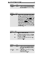
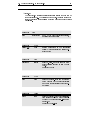
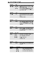
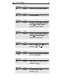
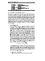
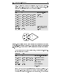
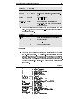
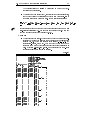
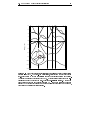
k-point set for a slab calculation
For a surface calculation with the z -axis as the surface normal, you want
the k-point mesh to lie in the xy-plane. There is no dispersion of the
electronic band structure of the slab in z -direction to sample. If there
would be, it just means that the repeated slabs are not decoupled as they
should be, i.e. the vacuum region was chosen too thin. Therefore the
z -coordinate of all k-points should be zero. The input typically looks
like
Parameter Value
nkpt
1
number of k-points supplied
xk(1..3)
0.5 0.5 0.0 1.0
k-points and weights
i facs(1..3) 8 8 1
k-point folding factors
frame of reference
t kpoint rel .true.
for k-points xk(1..3)
1
0
0
1
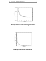
Figure 3.1: 2D Brillouin zone of a surface with cubic symmetry with a 8 8 MonkhorstPack grid. The thin square indicates the conventional rst Brillouin zone, the thick square
marks the Brillouin zone as realized in the fhi98md code. The location of one special
k-point (out of 64) within its tile is marked by the cross.
3.2 Choice of the k-point mesh
35
Note: We recommend to use even numbers for the folding parameters. As a
general rule, one should avoid using high symmetry points in the Brillouin zone
as sampling points, because this would result in an inferior sampling quality
at comparable numerical eort, compared to a similar number of o-axis kpoints. Conventionally (in contrast to our above denition), the Brillouin
zone is chosen to have the origin in its center. For odd numbers of the folding
parameters and the setting '0.5 0.5 . . . ', some of the 'unfolded' k-points will
fall on the zone boundary of the conventional Brillouin zone, which is often a
symmetry plane. Likewise, the k-point set may contain a periodic image of
the ;-point. This is normally undesirable.
❏
The concept of equivalent k-points
Usually one is not interested in the total energies themselves, but in comparing
dierent structures, i.e. accurate energy dierences are required. If the two
structures have the same unit cell, the comparison should always be done
using the same k-point set, so that possible errors from a non-converged kpoint sampling tend to cancel out. A similar strategy can also be applied when
comparing structures with dierent unit cells. We allude to this concept here
as 'equivalent k-point sampling': The structure with a large unit cell has
a smaller Brillouin zone associated with it. The k-points sampling along
this smaller Brillouin zone should be chosen as a subset of the k-point mesh
in the larger Brillouin zone, such that the position of the k-points in this
subset, expressed in Cartesian coordinates in reciprocal space, agree in both
calculations (to check whether this is actually the case, inspect the list of kpoints appearing in the inp.ini le). This goal can be achieved in a simple way
by choosing appropriate i facs. As an example, imagine you want to compare
two slab calculations, one with a (2 1), the other with a (4 2) unit cell. In
this case, use
Parameter
i facs(1..3)
in the rst case, and
Value
4 8 1
k-point folding factors
Parameter
Value
i facs(1..3)
2 4 1
k-point folding factors
in the second case, leaving the other parameters unchanged.
Note: b1 is orthogonal to the real lattice vectors a2 and a3 . If a1 is the long
edge of your real space unit cell, b1 spans the short edge of your Brillouin zone.
Therefore, the k-point sampling mesh has fewer points in the b1 direction and
more points in the b2 direction in the above example.
❏
Chadi-Cohen mesh
Another convention for choosing a k-point mesh has been proposed by Chadi
and Cohen [31], and has been applied to slab calculations by Cunningham[32].
In contrast to Monkhorst and Pack, the renement of the k-point mesh to obtain higher sampling density is based on a recursive scheme. However, for
cubic symmetry, the outcome of this algorithm can also be interpreted as
a special Monkhorst-Pack grid. To discuss dierences between the schemes,
we resort to the simple case of a two-dimensional mesh for a slab calculation. An example where Cunningham's scheme leads to results dierent from
Monkhorst-Pack are systems with hexagonal symmetry, e.g. slabs with (111)
surface of fcc-metals. Here, Cunningham proposes to use a hexagonal k-point
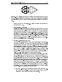
3.2 Choice of the k-point mesh
36
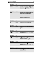
mesh. To realize such meshes in the fhi98md code, one has to provide explicitly a list of k-points forming the desired pattern. Cunningham's 6-point
pattern in the full Brillouin zone can be obtained as follows
Parameter
Value
nkpt
6
xk(1..3),wkpt 0.33333
xk(1..3),wkpt 0.66667
xk(1..3),wkpt 0.00000
xk(1..3),wkpt 0.00000
xk(1..3),wkpt 0.66667
xk(1..3),wkpt 0.33333
1 1 1
i facs(1..3)
t kpoint rel
.true.
0.00000 0.0 0.16667
0.00000 0.0 0.16667
number of k-points
k-points
and weights
0.33333 0.0 0.16667
0.66667 0.0 0.16667
0.33333 0.0 0.16667
0.66667 0.0 0.16667
k-point folding factors
frame of reference for
k-points
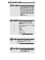
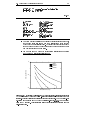
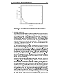
Figure 3.2: 2D Brillouin zone of a fcc(111) surface with hexagonal symmetry with set
of 6 special k-points following Cunningham. The thin polygon indicates the conventional
rst Brillouin zone, the thick polygon marks the Brillouin zone as realized in the fhi98md
code.
When a denser mesh in the same cell is desired, Cunningham's 18-point pattern is obtained from the input
Parameter
nkpt
xk(1..3),wkpt
xk(1..3),wkpt
i fa(1..3)
t kpoint rel
Value
2
0.3333 0.3333 0.0 0.5
0.6666 0.6666 0.0 0.5
3 3 1
.true.
number of k-points supplied
k-points and weights
k-points and weights
folding factors
frame of reference
for k-points
Here we have made use of the 'tiling' strategy employed in fhi98md. An
even denser k-point set, consisting of 54 points in the full Brillouin zone, may
be obtained by using the 6 k-points of the rst example, but as a pattern
3.2 Choice of the k-point mesh
37
Figure 3.3: 2D Brillouin zone of a fcc(111) surface with hexagonal symmetry with set
of 18 special k-points following Cunningham. The thin polygon indicates the conventional
rst Brillouin zone, the thick polygon marks the Brillouin zone as realized in the fhi98md
code.
repeated in each of the nine tiles, i.e. by setting the folding parameters in the
rst example to 3 3 1.
❏
❏
User-supplied k-point sets
In some cases (like a band structure calculation), the user might nd it more
convenient to specify the k-point mesh directly with respect to the coordinate
axes in reciprocal space, rather then with respect to the reciprocal lattice
vectors. This can be achieved by setting t kpoint rel to .false.. The unit of
length on the coordinate axes is 2=alat in this case. The folding parameters
can be used as well to enhance the number of k-points, if desired. However,
one should keep in mind that the k-point sets specied in that way might have
little symmetry, i.e. their number is not signicantly reduced by the built-in
symmetry reduction algorithm of fhi98start.
Reduced k-points and symmetry
Apart from the translational symmetry of the Bravais lattice, the crystal structure under investigation may often have additional point group symmetries.
These can be used to reduce the number of k-points which are needed in the
actual calculation (and thus the memory demand) substantially. To perform
the integrals in the Brillouin zone, it is sucient to sample the contribution
from a subset of non-symmetry-equivalent k-points only. Therefore the integrand (e.g. the charge density) is calculated only at these points. The
integrand with the full symmetry can be recovered from its representation by
non-symmetry-equivalent k-points whenever this is required.
The fhi98start utility is set up to automatically exploit these point group
symmetries. First, the point group symmetry operations applicable to the
unit cell are determined and stored in the form of symmetry matrices. Secondly, fhi98start seeks to reduce the elements of the k-point mesh to the q u
subset which is irreducible under those symmetry matrices. Only this subset
is forwarded in the inp.ini le for further use in the main computations. The
performance of the reduction procedure can be monitored by inspecting the
output in the le start.out. An estimate for the sampling quality of the k-point
set is given on the basis of the analysis of 'shells' (see Chadi and Cohen[31]
for details). For a good k-point set, the contribution from the leading 'shells'
should vanish. Some comments for interested users:
For a slab k-point set, those shells that contain contributions from lat-
tice vectors with a nite z-component cannot vanish, thus they must be
disregarded when judging the quality of the basis set.
3.3 Total Energy Minimization Schemes
38
The quality assessment only makes sense for systems with a band gap.
The eect of having a sharp integration boundary, the Fermi surface, for
a metal is not accounted for by Chadi and Cohen's shell analysis.
Note: Even if there are no point group symmetries, the vectors k and ;k are
symmetry-equivalent by virtue of time-inversion symmetry. For this reason,
the number of k-points is reduced by at least a factor of two for any reasonable
choice of a k-point mesh.
3.3 Total Energy Minimization Schemes
In an electronic structure calculation using a plane-wave basis, the Hilbert space
is typically spanned by a huge number of basis functions (up to 105 plane waves).
Therefore it would be unwise to attempt to diagonalize the Hamiltonian operator in
this high-dimensional space directly. Instead, one uses algorithms which only imply
vector operations on the wave function vector (in Hilbert space), rather than matrix
operations. The wave functions are gradually improved in an iterative process, until
they eventually converge towards the eigenvectors.
❏
Electronic minimization
The goal is to minimize the total energy with respect to the wave function
j i;k i starting with a trial wave function j i;(0)k i. The energy minimization
scheme is formulated in terms of an equation of motion for the wave function
j i;(tk) i in a ctitious time variable t.
Steepest Descent
The simplest scheme to iterate the wave functions is the steepest descent
approach [27]. It can be derived from a rst-order equation of motion
d j (t) i = ~ ; H^ j (t) i ;
i;k
KS
i;k
i;k
dt
imposing the ortho-normality constraint h i;(tk) j j;(tk) i = i;j , where H^ KS
is the Kohn-Sham Hamiltonian and ~i;k are the Lagrange multipliers
introduced to account for the ortho-normality constraint.
In the simplest possible discretization of this dierential equation, only
information from the last step is used,
hG + kj i;(tk+1) i = hG + kj i;(tk) i + hG + kj i;(tk) i ; hG + kjH^ KS j i;(tk) i
with = ~i;k t and = t. However, it turns out that this discretization
scheme is not very ecient.
Damped Joannopoulos
A more ecient scheme based on a second order equation of motion
might also be used
d2 j (t) i + 2 d j (t) i = ~ ; H^ j (t) i ;
i;k
KS
i;k
dt2 i;k
dt i;k
(3.1)
where is a damping parameter. The equation of motion is integrated
for a step length t by the Joannopoulos approach [28], which iteratively
improves the initial wave functions. In this algorithm the new wave
function j i;(tk+1) i is constructed from the wave functions of the last two
iteration steps t and (t ; 1)
hG + kj i;(tk+1) i = hG + kj i;(tk) i + G hG + kj i;(tk) i
;G hG + kj i;(tk;1) i ; G hG + kjH^ KS j i;(tk) i
3.3 Total Energy Minimization Schemes
39
where the coecients are
;t
^
G = ~i;k (hG (t) ; 1) ; hG +^kjHKS jG + ki e
~i;k ; hG + kjHKS jG + ki
;
t
G = e
hG (t) ; e;t ; 1
G =
~i;k ; hG + kjH^ KS jG + ki
with ~i;k = h i;(tk) jH^ KS j i;(tk) i. The function h(t) is dened by
8
< 2e; 2 t cos (!G t)
p
hG (t) = : ; t
2e 2 cosh j!2 j t
G
if !G2 0
if !G2 < 0
2
with !G2 = hG + kjH^ KS jG + ki ; ~i;k ; 4 .
Williams-Soler
Although the damped Joannopoulos algorithm is more ecient than the
rst order scheme, additional storage for the wave function j i;(tk;1) i is
needed. Therefore the Williams-Soler algorithm [29] is recommended
whenever storage requirements do not permit to employ the damped
Joannopoulos algorithm. The coecients of this scheme are
h
i
~i;k e(~i;k ;hG+kjH^ KS jG+ki)t ; 1
G =
~i;k ; hG + kjH^ KS jG + ki
(~i;k ;hG+kjH^ KS jG+ki)t ; 1
G = e
~i;k ; hG + kjH^ KS jG + ki
with G = 0. Thus, the damped Joannopoulos scheme contains the
Williams-Soler scheme as a limiting case, when ! 1. On the other
hand, the Williams-Soler scheme itself approaches the steepest descent
scheme, if t is suciently small.
The choice of t and depends on the atomic species and the conguration. The corresponding parameters in the inp.mod input le are delt
and gamma. Typically delt lies between 1 and 40 and gamma is within
the range 0 < < 1.
Set up the parameters delt, gamma, delt2 and gamma2 in the le inp.mod.
If the improvement in the total energy per iteration is less than
eps chg delt the parameters delt2 and gamma2 are used instead, in order
to ensure the stability of convergence. Note that the values for delta2
and gamma2 should be smaller than that ones for delta and gamma.
3.3 Total Energy Minimization Schemes
Parameter
delt
gamma
40
Type/Value
real > 1
0 < real < 1
Step length of electronic iteration
If i edyn =2 (see below), damping parameter
delt2
see delt
c.f. eps chg dlt
gamma2
see gamma
c.f. eps chg dlt
eps chg dlt real > 0
If the total energy varies less than
eps chg dlt, delt2 and gamma2 replace
delt and gamma
Choose the desired scheme to iterate the wave functions in the input
le inp.mod, setting up the parameter i edyn according to the following
numbers shown below.
Parameter
Value
i edyn
0
1
2
❏
Schemes to iterate the wave functions
steepest descent
Williams-Soler
damped Joannopoulos
Example
As an example we consider a total energy calculation for GaAs bulk in
the zinc-blende structure. The Williams-Soler minimization scheme is
used to iterate the wave functions and dierent values for the electronic
time step delt were used. The results are shown below. Note how the
convergence can be accelerated by changing the electronic time step delt.
The input les start.inp and inp.mod used for these calculations are
shown below.
start.inp
1
: number of processors
1
: number of minimal processors
1
: number of processors per group
2
: number of species
0
: excess electrons
4
: number of empty states
2 0
: ibrav pgind
10.68 0.0 0.0 1 1 1
: celldm
1
: number of k-points
0.5 0.5 0.5 1.0
: k-point coordinates, weight
4 4 4
: fold parameter
.true.
: k-point coordinates relative or absolute?
8 4.0
: Ecut [Ry], Ecuti [Ry]
0.1
.true. .f.
: ekt tmetal tdegen
.true. .false. 1
: tmold tband nrho
5 2 1234
: npos nthm nseed
873.0 1400.0 10000000 1: T_ion T_init Q nfi_rescale
.true. .false.
: tpsmesh coordwave
1 5 'Arsenic'
: number of atoms, zv, name
1.0 74.92 0.7 3 3
: gauss radius, mass, damping,l_max,l_loc
.t. .t. .f.
: t_init_basis
0.0 0.0 0.0 .f.
: tau0 tford
1 3 'Gallium'
: number of atoms, zv, name
3.3 Total Energy Minimization Schemes
1.0 69.72 0.7
.t. .t. .f.
0.25 0.25 0.25
3
.f.
3
41
: gauss radius, mass, damping,l_max,l_loc
: t_init_basis
: tau0 tford
inp.mod
-1 100 1000000
: nbeg
iprint timequeue
100 1
: nomore nomore_init
10.0 0.2
: delt gamma
4.0
0.3 0.0001
: delt2 gamma2 eps_chg_dlt
400 2
: delt_ion nOrder
0.0 1.0
: pfft_store mesh_accuracy
2 2
: idyn i_edyn
0 .false.
: i_xc t_postc
.F. 0.001 .F. 0.002
: trane ampre tranp amprp
.false. .false. .false. 1800 : tfor tdyn tsdp nstepe
.false.
: tdipol
0.0001 0.0005 0.3
: epsel epsfor epsekinc
0.001 0.001 3
: force_eps max_no_force
2
: init_basis
We attach a table containing some values to the electronic time step delt,
the damping parameter gamma and the minimization method adopted
which have been successfully used. Of course this table provides only a
few numbers and should be used only as rough guide as everyone has to
nd her/his "optimum" parameters.
For an example of a geometry optimization calculation see Section
How to set up a structural relaxation run.
−5
ln(E−E0)(Hartree)
delt=5
delt=10
delt=20
delt=40
−10
−15
0
20
Electronic time steps
40
Figure 3.4: A total energy calculation for GaAs bulk in the zinc-blende structure within
LDA approximation by using the Williams-Soler minimization scheme to iterate the wave
functions. Dierent values for the electronic time step delt are used. The Monkhorst-Pack
k-points mesh was taken as 444 with the initial k-point (0.5,0.5,0.5) and an energy
cuto of 8 Ry was used. E0 is the limiting value of the total energy approached in a very
well-converged run.
3.3 Total Energy Minimization Schemes
42
Table 3.1: Electronic time step delt, damping parameter gamma and minimization
schemes used for some bulk and slab (with and without adsorbates) calculations. The
labels J, WS and SD mean that either the damped Joannopoulos or Williams-Soler or
Steepest Descent minimization scheme was employed. The dimension along the z direction
is given by dim(z).
Bulk
Material
Si
GaAs
GaAs
GaN
Al
Al
Ag
Pt
Number of atoms
Scheme
delt
gamma
2
2
64 (defect)
4
1
1
1
1
J
J
J
WS
WS
SD
J
J
30
20
6
4
6
12
5
2
0.4
0.3
0.3
{
{
{
0.2
0.3
Material Number
of atoms
Si
70
GaAs
70
GaAs
96
GaN
70
Ag
66
Ag
7
Ru
21
Slab
z)
Adsorbates dim(
(Bohr)
H
43
In
35
35
In, As
40
Ag
64
64
CO, O
54
gamma
Scheme
delt
J
WS, J
J
WS
J
J
J
12
0.4
4{12 0.18{0.3
6
0.3
4
{
4
1
2
0.3
2
0.2
3.4 How to set up a structural relaxation run
43
3.4 How to set up a structural relaxation run
❏
Structural optimization schemes
The present program provides two methods to nd the equilibrium geometry,
namely the modied steepest descent scheme and the damped Newton scheme.
In the damped Newton scheme, the ions whose coordinates are given in the
input le start.inp are relaxed according to the iterative scheme
I(sn;Iita+1) = I(sn;Iita) + Is (I(sn;Iita) ; I(sn;Iita;1) ) + Is FIs ;Ia (fI(sn;Iita) g)
where Is and Is are the damping and mass parameters, respectively. Note
that these parameters determine whether the ions lose their initial potential
energy slowly in an oscillatory-like motion or whether they move straight into
the closest local minimum as in the modied steepest descent scheme.
❏
Pre-settings
Structural optimization run
The program has switches (tfor and tdyn) in inp.mod for setting up a
structural relaxation, a molecular dynamics calculation, or an electronic
structure calculation. The following table shows how to set up a structural relaxation.
Parameter
tfor
tdyn
Value
.true.
.false.
relaxation of ionic positions (c.f.
epsfor, force eps, and tford)
Choosing the structural optimization scheme
Set the parameter tsdp in inp.mod to choose which structural optimization scheme will be used.
Parameter
tsdp
Value
.true.
.false.
modied steepest descent scheme (currently not supported)
damped Newton scheme
Initial ionic coordinates and ag
The initial ionic coordinates for all ions in the supercell have to be given
and the ag which determines whether the ions may move has to be set.
Parameter
tau0(1..3)
tford
Type/Value
3 real
.true.
.false.
Mass and damping parameters
ion coordinates
the ions move
the ions do not move
The mass and damping parameters (ion fac and ion damp) determine
how the ions lose their initial potential energy (c.f. structural optimization schemes)
3.4 How to set up a structural relaxation run
Parameter
ion fac
Value
0.3{2
ion damp
0.4{0.7
44
mass parameter (tfor = .true. ). Note:
it is the ionic mass in [amu] if tdyn =
.true.
and tfor = .false.
damping parameter if tfor = .true.
and tdyn = .false. Note: it is used only
when tsdp = .false.
Force convergence parameters
The calculation of the electron ground state for a xed conguration of
the ions is terminated if the improvement of the total energy and the wave
functions per iteration is smaller than epsel and epsekinc, respectively.
However, for a structural relaxation calculation, the residual forces acting
on the ion should also be suciently small (smaller than epsfor). The
error of the forces (force eps(1)) is monitored (in the subroutine fionsc)
before performing a structure optimization step.
Parameter
epsfor
Value
0.0005
force eps(1)
0.001{0.1
forces on ions with tford = .true. must
be smaller than this criterion
maximum allowed relative variation in local forces before, if tfor = .true. and
tdyn = .false., executing a geometry optimization step or if tfor = .false. and
tdyn = .true., calculating total forces
Other parameters
timequeue is the maximum cpu time in seconds. nomore is the maximum number of atomic moves. nstepe is maximum number of electronic
iterations allowed to converge forces. If the forces on the ions do not
converge to the criterion force eps(1) after nstepe iterations, then the
program terminates. The maximum number max no force of electronic
iterations for which no local forces shall be calculated after each ionic
step (move) should also be set.
❏
Example
The example presented here is the structure optimization of the
GaAs(110) cleavage surface. The start atomic coordinates are at the
ideal bulk positions. The les start.inp and inp.mod are given below.
start.inp
1
: number of processors
1
: number of minimal processors
1
: number of processors per group
2
: number of species
0
: excess electrons
5
: number of empty states
8 0
: ibrav pgind
7.403408 10.47 51.823856 0 0 0 : celldm
1
: number of k-points
0.5 0.5 0.0 1.0
: k-point coordinates, weight
4 4 1
: fold parameter
3.4 How to set up a structural relaxation run
.true.
10 4.0
0.004 .true. .f.
.true. .false. 1
5 2 1234
873.0 1400.0 1e8 1
.t. .true.
9 3 'Gallium'
1.0 1.000 0.7 3 3
.t. .t. .f.
0.00000
3.701704
0.00000
3.701704
0.00000
3.701704
0.00000
3.701704
0.00000
9 5 'Arsenic'
1.0 1.000 0.7 3 3
.t. .t. .f.
3.701704
0.00000
3.701704
0.00000
3.701704
0.00000
3.701704
0.00000
3.701704
45
:
:
:
:
:
:
:
:
:
:
k-point coordinates relative or absolute?
Ecut [Ry], Ecuti [Ry]
ekt tmetal tdegen
tmold tband nrho
npos nthm nseed
T_ion T_init Q nfi_rescale
tpsmesh coordwave
number of atoms, zv, name
gauss radius, mass, damping,l_max,l_loc
t_init_basis
0.00000
-14.806816
.t.
5.23500
-11.105112
.t.
0.00000
-7.403408
.t.
5.23500
-3.701704
.f.
0.00000
0.00000
.f.
5.23500
3.701704
.f.
0.00000
7.403408
.t.
5.23500
11.105112
.t.
0.00000
14.806816
.t.
: number of atoms, zv, name
: gauss radius, mass, damping, l_max,l_loc
: t_init_basis
2.61750
-14.806816
.t.
7.85250
-11.105112
.t.
2.61750
-7.403408
.t.
7.85250
-3.701704
.f.
2.61750
0.00000
.f.
7.85250
3.701704
.f.
2.61750
7.403408
.t.
7.85250
11.105112
.t.
2.61750
14.806816
.t.
inp.mod
-1 20 1000000
1000 1
2.0 0.2
1.0 0.2 0.0001
400 2
0.0 1.0
2 2
0 .false.
.F. 0.001 .F. 0.002
.true. .false. .false. 100
.false.
0.0001 0.0005 0.1
0.001 0.001 3
1
❏
: nbeg
iprint timequeue
: nomore nomore_init
: delt gamma
: delt2 gamma2 eps_chg_dlt
: delt_ion nOrder
: pfft_store mesh_accuracy
: idyn i_edyn
: i_xc t_postc
: trane ampre tranp amprp
: tfor tdyn tsdp nstepe
: tdipol
: epsel epsfor epsekinc
: force_eps max_no_force
: init_basis
Analysis
After a job is executed, you have to check whether it has been nished
properly and the program has arrived at the optimized geometry. You should
check:
The dierence between the total energy and the Harris energy. The
dierence should be very small, e.g. 10;5 Hartree.
CPU time limit|Structural relaxation usually takes a lot of CPU time,
and in most cases it stops because the CPU time limit is out
The total energy convergence (see Fig. 3.5)
Mean force on ions (see Fig. 3.6)
Mean displacement per coordinate (see Fig. 3.7)
3.4 How to set up a structural relaxation run
46
Energy (Hartree)
−257.38
−257.39
−257.4
−257.41
0
500
1000
iterations
1500
Figure 3.5: Total energy as a function of electronic self-consistency iterations
0.01
mean force (Hartree/a.u.)
0.008
0.006
0.004
0.002
0
0
50
100
ionic steps
150
200
Figure 3.6: Mean force on ions as a function of ionic steps
3.4 How to set up a structural relaxation run
47
mean displacement (a.u.)
0.008
0.006
0.004
0.002
0
0
50
100
ionic steps
150
200
Figure 3.7: Mean displacement per coordinate as a function of ionic steps
❏
constraint relaxation
The present program also allows the user to constrain the motion of the atoms
during a structural optimization. For example, an atom adsorbing on a surface
may be allowed to relax in the xy-plane, but not along the z direction. An
adsorbing molecule may be allowed to rotate and to move in the xy-plane,
but its center of mass may not be allowed to move in the z direction. When
such constraints on the atomic motion are being set up, the location of the
\center of mass" of a group of atoms is determined by atomic weights chosen
by the user. These atomic weights do not have to be proportional to the
actual atomic masses of the atoms.
The information concerning the desired constraints on the atomic motion is
given in the le constraints.ini, which is used by the start program. The rst
line of this le contains the number of single-atom constraints, nr constraints .
One line for each of these constraints must follow, containing the vector direction along which the atom is not allowed to move, vec(j), j = 1; 3, followed by
the species number, is, and the atom number, ia. In the sample constraints.ini
le below, we see that three single-atom constraints are being set up. Atom
number 31 of species number 1 is not allowed to move in the [110] direction,
and atom number 32 of species number 1 is not allowed to move in the [001]
direction or the [010] direction.
The second part of the le constraints.ini must contain a line with the number
of center-of-mass-type constraints, nconstr , followed by a short section for
each constraint. The section for constraint i begins with a line giving the
number of atoms which are involved in this constraint, natm(i), followed by
the vector direction along which the "center of mass" of this group of atoms is
not allowed to move. One line follows for each atom in the group, giving the
weight of this atom in determining the "center of mass" position, constrw(i,k),
and the species and atom number, which are contained in the array iatm(i,k,l),
l = 1; 2. In the example le below, there is one center-of-mass-type constraint,
which involves the motion of two atoms. The "center of mass" of this twoatom group is not allowed to move in the [001] direction. The two atoms in
this group are atoms number 29 and 30 of species number 2, and both are
3.5 How to set up a continuation run
48
weighted equally in determining the "center of mass" position.
We note that if a particular atom is included in a center-of-mass-type constraint, this atom should not be included in any other constraints involving a
dierent group of atoms. This has not been a serious restriction in the past,
since the most useful applications tend to involve at most one center-of-masstype constraint.
constraints.ini
3
1
0
0
1
2
0.5
0.5
1
0
1
0
1
0
1
1
1
0
2
2
0
29
30
1
31
32
32
:nr_constraints
:{vec(j),j=1,3},is,ia
:{vec(j),j=1,3),is,ia
:{vec(j),j=1,3),is,ia
:nconstr
:natm(i), {constrv(i,j),j=1,3}
:constrw(i,k), {iatm(i,k,l), l=1,2}
:constrw(i,k), {iatm(i,k,l), l=1,2}
3.5 How to set up a continuation run
Under certain circumstances it might be desirable to continue a previous calculation,
because
the run-time in the queuing system of your hardware was too short to fully
converge the calculation
the calculation terminated prematurely due to some computer problem
the plane-wave cut-o or the number of k-points needs to be increased to
ascertain convergence with respect to these parameters.
Restart les in binary format are written every iprint self-consistency cycles (c.f.
inp.mod). The le fort.71 contains the wave functions and the coordinates of the
ions, as well as all other information required for a restart. The electron density is
stored in the le fort.72.
❏
General continuation run, or run with increased cut-o
The following parameters need to be reset for performing continuation runs.
Notice that some parameters may be set in start.inp or, likewise, in inp.ini.
In the latter case, running the fhi98start program can be omitted.
Rename the le fort.71 into fort.70.
In the le inp.mod, set the parameter nbeg to -2.
In the le inp.ini or start.inp, set nrho = 2, which causes the program
to constructs the initial electron density from fort.70. When nrho = 3,
it reads the initial electron density from fort.72 instead.
Usually one would also set coordwave = .true., which causes the program to read the last available ionic positions from fort.70. Otherwise
the program reads the ionic positions from inp.ini. This option would
allow the user to modify the ionic positions slightly between consecutive
runs.
Note that it is very ecient to use a previous wavefunction-le as fort.70 when
increasing the cut-o. In this case, only the additionally required plane-wave
coecients with larger wave number need to be recalculated. When doing so,
however, it is inevitable to rerun fhi98start to generate a modied inp.ini-le.
3.6 How to set up a band structure calculation
❏
49
Continuation run for a molecular dynamics simulation
Proceed like described above, in particular set coordwave = .true..
Rename the le fort.21 into fort.20.
In the le inp.ini or start.inp, set npos to 6. This causes the program to
read all required information to continue the ions' trajectories from the
(binary) le fort.20.
❏
Continuation run with increased k-point set, or band structure calculation
In the le inp.ini, set the parameter nrho to 3.
Make sure that the old output charge density in fort.72 is available.
In this case the wavefunctions need to be recalculated, therefore nbeg remains
to be equal to -1. Also, the program fhi98start needs to be rerun.
3.6 How to set up a band structure calculation
❏
Pre-settings
Before running fhi98md in band structure mode, do an ordinary total energy
run for the system of interest to get a well-converged electron density. The
latter is stored in fort.72. The unit cell should be chosen as follows:
Bulk band structure
Use the same bulk unit cell as the one for which the band structure will
be calculated. Usually this is the minimum cell, e.g. two atoms for Si or
GaAs.
Projected bulk band structure
To make the bulk unit cell rst take the same lateral unit cell as for the
surface, then take the minimum periodicity in the third direction. This
is required in order to have correspondence between the kk coordinates
for the bulk and the surface, respectively.
Surface band structure
Use the same surface unit cell as the one for which the band structure
will be calculated.
❏
Band structure run
Switch on the band structure run mode of fhi98md by setting the |indexemtband parameter in start.inp to .true..
Parameter
tband
Value
.true.
the k-point set is not reduced by
fhi98start utility; the electron density is
not recalculated after the initialization
Set the value of nrho parameter in start.inp to 3.
Parameter
nrho
Value
3
the initial electron density is read in from
fort.72
3.6 How to set up a band structure calculation
50
Sample the symmetry lines in the Brillouin zone along which you want to
calculate the energy bands|the resulting k-point set should be declared
in start.inp in the standard format (see also Choice of the k-point mesh).
Be sure to set the proper value for the t kpoint rel parameter in the
same le depending on the reference frame used to determine the k-point
coordinates (xk(1..3) parameters).
To avoid folding of the k-point set, all components of the i facs parameter
in start.inp should be set to 1.
Remember to take enough of empty states, parameter nempty in
start.inp, if you want to get the lowest unoccupied bands as well.
Parameter
i facs(1..3)
t kpoint rel
Value
k-points folding factors: no folding
k-points are given in Cartesian coordi-
1 1 1
.false.
nates in units 2=alat
frame of reference for k-points is spanned
by the reciprocal lattice vectors, i.e. k =
k1 b1 + k2 b2 + k3 b3
.true.
Projected bulk band structure
Calculate the bulk band structure for the same set of kk points as for the
surface for which you want to project the bulk bands, but with k? going
from ;2=a? to 2=a?; where a? is the unit cell size in the perpendicular
to the surface direction. If the symmetry of your system includes a mirror
plane parallel to the surface then it is sucient to take only half of the
interval, e.g. k? 2 [0; 2=a?]:
Other parameters
epsekinc (inp.mod): use this parameter to control the eigenvalues'
convergence.
♦
❏
Analysis
The k-point coordinates together with the corresponding sorted KohnSham eigenvalues (in eV) and occupation numbers are listed at the end of
the output le fort.6 (see Example section). For example, the following
command line on UNIX systems would extract the eigenvalues to the le
eigenvalues.dat:
grep '^>eig:' fort.6 | sed 's/>eig://g' > eigenvalues.dat
Alternatively, the k-points coordinates ki ; weights wki and the corresponding eigenvalues together with some additional information are
saved in the le report.txt in the format:
...
[number of k-points]
ki1
"i1
..
.
"iN
...
ki2
ki3
wki
report.txt
[number of eigenvalues per k-point N ]
3.6 How to set up a band structure calculation
51
The parallel version of fhi98md writes also an output le fort.3
containing the eigenvalues.
The value of the Fermi energy in eV, respectively the Fermi level location,
can be traced during the calculation and picked from the Efermi-eld of
the information record written to fort.6 at each electronic iteration:
...
>>>n_it nfi
... Etot
>>> 23 0
... -8.29527
...
Eharr
-8.44641
Ezero
mForce
-8.29527
.00000
mChange
.000
Seq
.0000
Sneq
.0000
Efermi
2.6057
It is important to remember that the Fermi energy should be taken from a real
self-consistent calculation (e.g. the one used to generate the fort.72 le) and
not from the band structure run (see also Fig. 3.8).
❏
Example
The sample input le start.inp below sets up a bulk band structure calculation for GaAs along the standard symmetry lines of the Brillouin zone
(inset in Fig. 3.8) of the face centered cubic lattice L-;-X-W-K-; (40
equidistant k-points, nkpt = 40). Note that with the number of empty
states nempty = 5 the ve lowest unoccupied bands will be calculated as
well. By setting t kpoint rel = :false: one guarantees that the k-point
coordinates will be used exactly as specied.
start.inp
1
1
1
2
0
5
2 0
10.682 0.0
40
0.5
0.4422650
0.3845300
0.3267950
0.2690600
0.2113250
0.1535900
0.0958548
0.0381198
0
0.1
0.2
0.3
0.4
0.5
0.6
0.7
0.8
0.9
1.
1.
1.
1.
1.
1.
0.9292890
0.8585790
0.7878680
0.75
0.6792890
0.6085790
0.5378680
0.0 0 0 0
0.5
0.4422650
0.3845300
0.3267950
0.2690600
0.2113250
0.1535900
0.0958548
0.0381198
0
0
0
0
0
0
0
0
0
0
0
0.1
0.2
0.3
0.4
0.5
0.5707110
0.6414210
0.7121320
0.75
0.6792890
0.6085790
0.5378680
: number of processors
: number of minimal processors
: number of processors per group
: number of species
: excess electrons
: number of empty states
: ibrav pgind
: celldm
: number of k-points
0.5
0.025
:--- L --------0.4422650 0.025
:
|
0.3845300 0.025
:
0.3267950 0.025
:
P
0.2690600 0.025
:
a
0.2113250 0.025
:
t
0.1535900 0.025
:
h
0.0958548 0.025
:
0.0381198 0.025
:
i
0
0.025
:--- Gamma
n
0
0.025
:
0
0.025
:
t
0
0.025
:
h
0
0.025
:
e
0
0.025
:
0
0.025
:
B
0
0.025
:
r
0
0.025
:
i
0
0.025
:
l
0
0.025
:--- X
l
0
0.025
:
o
0
0.025
:
i
0
0.025
:
n
0
0.025
:
0
0.025
:--- W
Z
0
0.025
:
o
0
0.025
:
n
0
0.025
:
e
0
0.025
:--- K
0
0.025
:
|
0
0.025
:
|
0
0.025
:
|
Dvolt ...
.0000 ...
3.6 How to set up a band structure calculation
0.4671570 0.4671570
0.3964470 0.3964470
0.3257360 0.3257360
0.2550250 0.2550250
0.1843150 0.1843150
0.1136040 0.1136040
0.0428932 0.0428932
0
0
1 1 1
.false.
8.0 4.0
0.005 .true. .false.
.true. .true. 1
5 2 1234
873.0 1400.0 1e8 1
.true. .true.
1 3 'Gallium'
1.0 3.0 0.7 3 3
.t. .t. .f.
0.0 0.0 0.0
.f.
1 5 'Arsenic'
1.0 3.0 0.7 3 3
.t. .t. .f.
0.25 0.25 0.25 .f.
52
0
0
0
0
0
0
0
0
:
:
:
:
:
:
:
:
0.025
:
|
0.025
:
|
0.025
:
|
0.025
:
|
0.025
:
|
0.025
:
|
0.025
:
|
0.025
:--- Gamma ----fold parameter
k-point coordinates relative or absolute?
Ecut [Ry], Ecuti [Ry]
ekt tmetal tdegen
tmold tband nrho
npos nthm nseed
T_ion T_init Q nfi_rescale
tpsmesh coordwave
: number of atoms, zv, name
: gauss radius, mass, damping,l_max,l_loc
: t_init_basis
: tau0 tford
: number of atoms, zv, name
: gauss radius, mass, damping, l_max,l_loc
: t_init_basis
: tau0 tford
A sample output le fort.6 generated by fhi98md using input from the
start.inp le above.
fort.6
---------------------------------------------------******* This is the complex fhi98md program ********
*******
February 1999
********
--------------------------------------------------->>>nbeg= -1 nomore=
100 iprint= 50
>============================================
> Exchange/Correlation: LDA
>============================================
>>>electronic time step= 20.0000 gamma=
.2000
>>> Using delt=
8.0000 gamma=
.2000 when energy changes less than:
.1000E-03
>accuracy for convergency: epsel= .00001 epsfor= .00050 epsekinc= .10000
>schultze algorithm for electron dynamics
>ions are not allowed to move
normally no mixing of old charge is done
N. B.: The same atom should not be involved in
more than one center-of-mass-type constraint.
>ibrav= 2 pgind= 0 nrot= 24 alat= 10.682 omega= 304.7177 mesh=
14
14
14
>ecut=
8.0 ryd
ecuti=
4.0 ryd
nkpt= 40
nel, tmetal, ekt, tdegen= 8.00000000000000000 T 0.500000000000000010E-02 F
>alat=
10.682000 alat=
10.682000 omega= 304.717734
Lattice vectors
a1
-5.341000
.000000
5.341000
a2
.000000
5.341000
5.341000
a3
-5.341000
5.341000
.000000
Reciprocal lattice vectors
b1
-1.000000
-1.000000
1.000000
b2
1.000000
1.000000
1.000000
b3
-1.000000
1.000000
-1.000000
Atomic positions tau0 :
Species
Nr.
x
y
z
Galium
1
.0000
.0000
.0000
Arsenic
1
2.6705
2.6705
2.6705
Number of kpoints: nkpt = 40
Ratios of FFT mesh dimensions to sampling theorem 1.029 1.029 1.029
>ps-pots as given on radial mesh are used
>gvk: ngwx and max nr. of plane waves:
134
125
k-point
weight
# of g-vectors
1
.50
.50
.50
.0010
120
2
.44
.44
.44
.0010
114
.....
40
.00
.00
.00
.0010
113
Weigthed number of plane waves npw:
116.221
Ratio of actual nr. of PWs to ideal nr.:
.99816
# of electrons=
8.0000, # of valencestates=
4, # of conduction states=
5
3.6 How to set up a band structure calculation
53
atomic data for 2
atomic species
pseudopotentialparameters for Galium
>nr. of atoms:
1, valence charge: 3.000, force fac: 3.0000, speed damp: .7000
l_max 3 l_loc: 3 rad. of gaussian charge: 1.000
pseudopotentialparameters for Arsenic
>nr. of atoms:
1, valence charge: 5.000, force fac: 3.0000, speed damp: .7000
l_max 3 l_loc: 3 rad. of gaussian charge: 1.000
Final starting positions:
.0000
.0000
.0000
2.6705 2.6705 2.6705
phfac: is, n_ideal: 1
0
phfac: is, n_ideal: 2
0
phfac:is,i_kgv,n_class 1 0 0
phfac:is,i_kgv,n_class 2 0 0
>nlskb:is= 1 wnl: 1
-.4019882 2 -2.8405414 3 -2.8405414 4 -2.8405414
>nlskb:is= 2 wnl: 1
-.3798314 2 -1.6212706 3 -1.6212706 4 -1.6212706
-------------------------------------------starting density calculated from pseudo-atom
-------------------------------------------formfa: rho of atom in 3.000000
formfa: rho of atom in 5.000000
ELECTRON DENSITY WILL NOT BE UPDATED
DURING CALCULATIONS.
=======================================================
SYMMETRY OPERATIONS
=======================================================
>s(isym) in latt. coord:
>sym(..) in cart. coord:
.....
>sym(..) in cart. coord:
1
1.00000
0
.00000
0
.00000
0
.00000
1
1.00000
0
.00000
0
.00000
0
.00000
1
1.00000
-1.00000
.00000
.00000
.00000
1.00000
.00000
.00000
.00000 -1.00000
=======================================================
CHECK SYMMETRIES
=======================================================
>Center of symmetry sym0=
.000000
.000000
Table of symmetry relations of atoms,
is ia iasym isym
tau0
xneu
1
1
1
1
.00000
.00000
.00000
.....
2
1
1
24
2.67050 2.67050 2.67050
.000000
(iasym=nr. of symmetric at., xneu=tau0+<sym.Op.(isym)>)
.00000
-2.67050
.00000
.00000
2.67050 -2.67050
=======================================================
ITERATIONS IN INIT STARTED
=======================================================
1 iterations will be performed in the initialization
-1 ----- initialization loop ------------------------------------------------------ik= 1
Number of plane waves
= 40
Number of localized orbitals
= 8
Total number of states for initialization= 48
==== time consumption for a single k-point ====
time used for mapping of G-G`
=
.00
time used for creation of B0
=
.35
time used for <G+k|H_nl|G`+k>
=
.03
time used for <G+k|H_loc|G`+k> =
.00
time used for <BG|H|BG`>
=
.04
time used for diagonalization
=
.02
================================================
.....
---------------------------------------ik= 40
Number of plane waves
= 51
Number of localized orbitals
= 8
Total number of states for initialization= 59
nel
dfmax
fscale
efermi
ekt
8.00000
.030
1.00000
2.60750
.005
k-point
.500 .500 .500, eigenvalues and
eig -8.584 -4.211
.991
.991 3.318 7.045
occ 2.0000 2.0000 2.0000 2.0000 .0000 .0000
.....
k-point
.000 .000 .000, eigenvalues and
eig -10.005 2.030 2.030 2.030 2.781 6.232
occ 2.0000 2.0000 2.0000 2.0000 .0000 .0000
>>>
1 -10.8263451 -7.7123788
time per tb-loop
=
18.49
seq
.00000
sneq
.00000
occupation numbers:
7.045 10.305 12.535
.0000 .0000 .0000
6.232
.0000
6.232
.0000
occupation numbers:
9.962
.0000
3.6 How to set up a band structure calculation
54
total time for
1 loops
=
18.49
init stores starting density for mixing in c_fft_store
time elapsed for init:
26.8600
total number of wave function components: 4652
=======================================================
ITERATIONS IN MAIN STARTED
=======================================================
=== LOOP n_it= 1
time elapsed for nlrh t =
.0300
RHOE read from unit7 in RHOOFR.
Number of electrons in real space: 7.99999630944237516
time elapsed for rhoofr t =
.0000
internal energy at zero temperature
non-equillibrium entropy
equillibrium entropy
kT energy
(non-eq) free energy
(non-eq) total energy
Harris energy
kinetic energy
electrostatic energy
real hartree energy
pseudopotential energy
n-l pseudopotential energy
exchange-correlation energy
exchange-correlation potential energy
kohn - sham orbital energy
self energy
esr energy
gaussian energy
=
=
=
=
=
=
=
=
=
=
=
=
=
=
=
=
=
=
-8.305721
.000000
.000000
.005 eV
-8.305721
-8.305721
-8.451691
3.225369
-10.000821
.763345
1.472645
-.632887
-2.370027
-3.090283
-.739312
13.564038
.000048
5.801080
a.u.
kB
kB
a.u.
a.u.
a.u.
a.u.
a.u.
a.u.
a.u.
a.u.
a.u.
a.u.
a.u.
a.u.
a.u.
a.u.
===================================================
&&s atomic positions and local+nl forces on ions:
Galium
:
Arsenic
:
time elapsed for vofrho t =
.0600
time elapsed for n x
nkpt x graham/ortho =
.2200
nel
dfmax
fscale
efermi
ekt
seq
sneq
8.00000
.030
.40000
2.60750
.005
.00000
.00000
.....
>>>n_it nfi
Ekinc
Etot
Eharr
Ezero
mForce
mChange
>>> 1 0
2.70633
-8.30572
-8.45169
-8.30572
.00000
.000
(I finished storing wavefunctons and data on fort.71)
>>> OK, I stop after timestep nr. 10000
time elapsed per electronic time step t =
1.9200
time in queue:
14400 max. number of steps:
7111
>>> 2 0
2.83522
-8.30155
-8.44343
-8.30155
.00000
.000
.....
>>> 22 0
.09358
-8.29527
-8.44641
-8.29527
.00000
.000
=== LOOP n_it= 23
phfac: is, n_ideal: 1
0
phfac: is, n_ideal: 2
0
RHOE read from unit7 in RHOOFR.
Number of electrons in real space: 7.99999630944237516
internal energy at zero temperature
non-equillibrium entropy
equillibrium entropy
kT energy
(non-eq) free energy
(non-eq) total energy
Harris energy
kinetic energy
electrostatic energy
real hartree energy
pseudopotential energy
n-l pseudopotential energy
exchange-correlation energy
exchange-correlation potential energy
kohn - sham orbital energy
self energy
esr energy
gaussian energy
=
=
=
=
=
=
=
=
=
=
=
=
=
=
=
=
=
=
-8.295270
.000000
.000000
.005 eV
-8.295270
-8.295270
-8.446409
3.225369
-10.000821
.763345
1.472645
-.622437
-2.370027
-3.090283
-.640411
13.564038
.000048
5.801080
===================================================
a.u.
kB
kB
a.u.
a.u.
a.u.
a.u.
a.u.
a.u.
a.u.
a.u.
a.u.
a.u.
a.u.
a.u.
a.u.
a.u.
Seq
.0000
Sneq
Efermi
Dvolt
W_a
.0000
2.6075
.0000
.0000
.0000
.0000
2.6057
.0000
.0000
.0000
.0000
2.6057
.0000
.0000
3.6 How to set up a band structure calculation
55
&&s atomic positions and local+nl forces on ions:
Galium
:
>&&s-n
.000000
.000000
.000000
.000000
.000000
.000000
Arsenic
:
>&&s-n
2.670500
2.670500
2.670500
.000000
.000000
.000000
>sum of all (local+nl) forces / n_atoms =
.0000000000
.0000000000
.0000000000 (should = 0)
nel
dfmax
fscale
efermi
ekt
seq
sneq
8.00000
.030
.40000
2.60571
.005
.00000
.00000
> 1. k-point
.500 .500 .500, ngw
120
>Eigenvalues and Occupations:
>eig: -8.164 -4.000 1.350 1.350 3.484 7.111 7.111 10.332 12.784
>occ: 2.0000 2.0000 2.0000 2.0000 .0000 .0000 .0000 .0000 .0000
.....
> 40. k-point
.000 .000 .000, ngw
113
>Eigenvalues and Occupations:
>eig: -9.667 2.453 2.453 2.453 3.041 6.239 6.239 6.239 9.894
>occ: 2.0000 2.0000 2.0000 2.0000 .0000 .0000 .0000 .0000 .0000
>>>n_it nfi
Ekinc
Etot
Eharr
Ezero
mForce
mChange
>>> 23 0
.09107
-8.29527
-8.44641
-8.29527
.00000
.000
(I finished storing wavefunctons and data on fort.71)
================= END OF THE MAIN-LOOP ===================
average time elapsed for nlrh
:
.0287
rhoofr
:
.0000
vofrho
:
.0457
n x nkpt x dforce
:
1.5991
nkpt x graham/ortho :
.2217
rest (in main)
:
.0226
per elec. time step
:
1.9178
Seq
.0000
Sneq
Efermi
Dvolt
W_a
.0000
2.6057
.0000
.0000
3.6 How to set up a band structure calculation
56
8
6
4
2
Energy (eV)
0
−2
−4
kz
−6
L
Λ
−8
∆
Γ
Σ
K
Q
U
Σ'
W Z
X
ky
kx
−10
−12
−14
L
Γ
X
W
K
Γ
Figure 3.8: GaAs bulk band structure calculated with fhi98md within the local density
approximation (LDA). The Kohn-Sham eigenvalues, extracted from the above output le
, are denoted by () and the Brillouin zone of the fcc lattice is shown in the inset.
The energy is measured with respect to the EFermi (dashed line) obtained from the selfconsistent run used to produce the
le (see Pre-settings section). Note that in
case of systems with gap in the energy spectrum EFermi in a band structure run is only
assured to be between the valence band maximum and the conduction band minimum,
thus having no particular physical meaning.
fort.6
fort.72
Bibliography
P. Hohenberg and W. Kohn, Phys. Rev. 136B, 864 (1964).
W. Andreoni, F. Gygi, and M. Parrinello, Phys. Rev. Lett. 68, 823 (1992).
N. Troullier and J. L. Martins, Phys. Rev. B 46, 1754 (1992).
G. Ortiz, Phys. Rev. B 45, 11328 (1992).
A. Garcia et al., Phys. Rev. B 46, 9829 (1992).
S. B. Zhang and J. E. Northrup, Phys. Rev. Lett. 67, 2339 (1991).
M. Fuchs, M. Bockstedte, E. Pehlke, and M. Scheer, Phys. Rev. B 57, 2134
(1998).
[8] J. Neugebauer and M. Scheer, Phys. Rev. B 46, 16067 (1992).
[9] R. Stumpf and M. Scheer, Phys. Rev. B 53, 4958 (1996).
[10] C. Stamp and M. Scheer, Phys. Rev. Lett. 78, 1500 (1997).
[11] P. Kratzer, E. Pehlke, M. Scheer, M. B. Raschke, and U. Hofer, Phys. Rev.
Lett. 81, 5596 (1998).
[12] T. K. Zywietz, J. Neugebauer, and M. Scheer, Appl. Phys. Lett. 74, 1695
(1999).
[13] G. B. Bachelet, D. R. Hamann, and M. Schluter, Phys. Rev. B 26, 4199 (1982).
[14] D. R. Hamann, Phys. Rev. B 40, 2980 (1989).
[15] N. Troullier and J. L. Martins, Phys. Rev. B 43, 1993 (1991).
[16] X. Gonze, R. Stumpf, and M. Scheer, Phys. Rev. B 44, 8503 (1991).
[17] L. Kleinman and D. M. Bylander, Phys. Rev. Lett. 48, 1425 (1982).
[18] D. M. Ceperley and B. J. Alder, Phys. Rev. Lett. 45, 567 (1980).
[19] J. P. Perdew and A. Zunger, Phys. Rev. B 23, 5048 (1981).
[20] A. D. Becke, Phys. Rev. A 38, 3098 (1988).
[21] J. P. Perdew, Phys. Rev. B 33, 8822 (1986).
[22] J. P. Perdew, J. A. Chevary, S. H. Vosko, K. A. Jackson, M. R. Pederson, D. J.
Singh and C. Fiolhais, 46, 6671 (1992).
[23] C. Lee, W. Yang and R. G. Parr, Phys. Rev. B 37, 785 (1988).
[24] J. P. Perdew, K. Burke and M. Ernzerhof, Phys. Rev. Lett. 77, 3865 (1996).
[1]
[2]
[3]
[4]
[5]
[6]
[7]
57
BIBLIOGRAPHY
58
[25] M. Bockstedte, A. Kley, J. Neugebauer and M. Scheer, Comput. Phys. Commun. 107, 187 (1997).
[26] M. Fuchs and M. Scheer, Comput. Phys. Commun. 119, 67 (1999).
[27] M. C. Payne et al., Rev. Mod. Phys. 64, 1045 (1992).
[28] M. C. Payne et al., Phys. Rev. Lett. 56, 2656 (1986).
[29] A. Williams and J. Soler, Bull. Am. Phys. Soc. 32, 562 (1987).
[30] H. J. Monkhorst and J. D. Pack, Phys. Rev. B 13, 5188 (1976).
[31] D. J. Chadi and M. L. Cohen, Phys. Rev. B 8, 5747 (1973).
[32] S. L. Cunningham, Phys. Rev. B 10, 4988 (1974).
Index
a1, 19
a2, 19
a3, 19
alat, 19
ampre, 6
amprp, 6
atom, 12
atoms, 3
movement of, 3
number of, 20, 42
fionsc,
5, 44
force eps(1), 7, 44
force eps(2), 7
fort.1, 26
fort.20, 3, 49
fort.21, 26, 49
fort.3, 51
fort.6, 24, 26
fort.70, 12
fort.71, 26, 48
fort.72, 5, 26, 48, 49
fort.73, 26
fort.74, 26
fort.80, 26
b1, 19
b2, 19
b3, 19
Brillouin zone, 33{37, 50{56
integrals in, 37
symmetry lines in, 50
broyd, 5
gamma, 7
gamma2, 7
i edyn, 8
i facs, 14, 50
i xc, 8
iatm, 47
ibrav, 13
idyn, 8
ineq pos, 19
init basis, 12
initbasis, 8
initialization, 3, 20
block, 3
mixed-basis-set, 3
inp.ini, 3, 18, 37, 48
inp.mod, 3, 6, 39, 43
ion damp, 13, 44
ion fac, 13, 44
iprint, 8, 48
celldm, 12
constraints.ini, 47
constrw, 47
coordwave, 12, 48
delt, 6
delt2, 6
delt ion, 6
dforce b, 5
ecut, 12
ecuti, 12
ekt, 13
energy, 26
eps chg dlt, 7
epsekinc, 7
epsel, 7
epsfor, 7, 44
fermi,
l loc, 14, 24
latgen, 31
lmax, 14, 24
5
fhi98md, 1
max basis n, 19
max no force, 9, 44
mesh, 19
Chadi-Cohen, 35
Fourier, 21
k-point, 33{38
'tiling' strategy in, 36
algorithms used in, 3
structure of the program, 3
fhi98pp package, 23
fhi98start, 1, 6, 49
fiondyn, 5
59
INDEX
Monkhorst-Pack, 33, 41
mesh accuracy, 9
minpes, 15
mmaxx, 19
n t store, 19
na, 14
natm, 47
nax, 20
nbeg, 9, 48
nconstr, 47
nel, 20
nel exc, 14
nempty, 14, 50
nempty, 25
n rescale, 14
ngrpx, 15
ngwix, 20
ngwx, 20
nkpt, 14
nlmax, 20
nlmax init, 20
nlrhkb b, 5
nnrx, 20
nomore, 9, 25
nomore init, 9
nOrder, 10
npes, 15
npos, 15
nr constraints, 47
nrho, 12, 15, 48, 49
nrot, 20
nrx, 21
nschltz, 21
nseed, 15
nsp, 15, 23
nstepe, 10, 44
nsx, 21
nthm, 16
nx, 21, 25
nx basis, 21
nx init, 21
o wave, 5
omega, 21
pt store, 10
pgind, 16
pgsym, 29
project, 5
pseudopotentials, 1, 19, 23
format of le(s), 23
ionic, 23
psgen tool, 23
60
Q, 16
report.txt, 26
rho psi, 5
rhoz, 26
run, 1
band structure, 49, 51, 56
continuation, 25, 48
for a MD simulation, 49
with increased k-point set, 49
structural relaxation, 43
s(3,3), 21
start.inp, 6, 12, 30, 43
start.out, 31, 37
status.txt, 26
stople, 3, 25
stopprogram, 5, 25
t coord auto, 22
T init, 16
t init basis, 16
T ion, 16
t kpoint rel, 17, 50
t postc, 10
tau0, 17, 31, 43
tband, 17
tdegen, 17, 25
tdipol, 10
tdyn, 10, 43
tfor, 11, 13, 43
tford, 43
timequeue, 11
tmetal, 17
tmold, 17
tpsmesh, 17, 23
trane, 6, 11
tranp, 11
tsdp, 11, 13, 43
vau0, 18
vec, 47
vofrho, 5
wkpt, 18
xk, 18, 50
zv, 18, 24