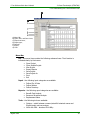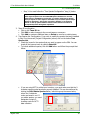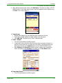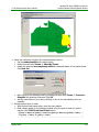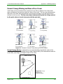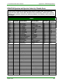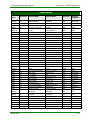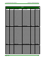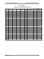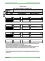
1
User’s Manual i-Tree Software Suite v2.1 Tools for assessing and managing Community Forests A cooperative initiative between: For more information, please visit http://www.itreetools.org i-Tree Software Suite User’s Manual Table of Contents i-Tree Software Suite User’s Manual Table of Contents Preface ........................................................................................................................ iv Acknowledgments....................................................................................................... vi 1. Ecosystem Analysis (UFORE) ................................................................................... 1 1.1 1.2 1.3 Introduction .......................................................................................................... 1 Installation ............................................................................................................ 2 Getting Started...................................................................................................... 2 1.3.1 Sampling Method and Data Collection ................................................................ 2 1.3.2 Opening the Sample UFORE Project ................................................................... 6 1.3.3 Creating a New UFORE Project .......................................................................... 6 1.3.4 Opening an Existing UFORE Project ................................................................... 8 1.3.5 Updating an Existing UFORE Project................................................................... 8 1.3.6 Understanding the UFORE Work Area ................................................................ 9 1.4 Data Operations .................................................................................................. 11 1.4.1 Minimum Field Data Requirements................................................................... 11 1.4.2 Air Pollution Data............................................................................................ 11 1.4.3 Automatic Data Transfer ................................................................................. 12 1.5 Reporting Results ................................................................................................ 13 1.5.1 General .......................................................................................................... 13 1.5.2 Maps (Beta) ................................................................................................... 14 1.5.3 Written Report................................................................................................ 20 1.6 Troubleshooting .................................................................................................. 20 1.7 Data Collection .................................................................................................... 20 1.7.1 Plot Information ............................................................................................. 21 1.7.2 Ground Cover Information............................................................................... 25 1.7.3 Shrub Information .......................................................................................... 25 1.7.4 Tree Information ............................................................................................ 26 2. Street Tree Analysis (STRATUM)............................................................................ 31 2.1 2.2 Introduction ........................................................................................................ 31 Installation .......................................................................................................... 32 2.2.1 System Requirements ..................................................................................... 32 2.2.2 Hardware Requirements.................................................................................. 32 2.2.3 Installing STRATUM ........................................................................................ 32 2.3 Getting Started.................................................................................................... 33 2.3.1 Choosing an Inventory Method and Formatting Data......................................... 33 2.3.2 Opening the Sample STRATUM Project............................................................. 34 2.3.3 Creating a New STRATUM Project .................................................................... 34 2.3.4 Opening an Existing STRATUM Project ............................................................. 35 2.3.4 Understanding the STRATUM Work Area .......................................................... 35 August 2008 i i-Tree Software Suite User’s Manual Table of Contents 2.4 Data Operations .................................................................................................. 38 2.4.1 Define City and Costs...................................................................................... 38 2.4.2 Define Species................................................................................................ 39 2.4.3 Define Inventory............................................................................................. 41 2.5 Reporting Results ................................................................................................ 42 2.5.1 Benefit - Cost Analysis Reports ........................................................................ 43 2.5.2 Resource Structural Analysis............................................................................ 43 2.5.3 Replacement Values........................................................................................ 46 2.5.4 Exporting Reports ........................................................................................... 46 2.5.5 Printing Reports.............................................................................................. 46 2.6 Troubleshooting .................................................................................................. 47 2.7 Data Collection .................................................................................................... 48 2.7.1 Collecting Data for a Full Inventory .................................................................. 48 2.7.2 Collecting Data for a Sample Inventory ............................................................ 48 3. Utilities ................................................................................................................... 50 3.1 Mobile Community Tree Inventory (MCTI)............................................................. 50 3.1.1 MCTI — Introduction ...................................................................................... 50 3.1.2 MCTI — Installation ........................................................................................ 51 3.1.3 MCTI — Getting Started .................................................................................. 52 3.1.4 MCTI — Data Operations................................................................................. 54 3.1.5 MCTI — Reporting Results............................................................................... 55 3.1.6 MCTI — Troubleshooting................................................................................. 56 3.1.7 MCTI — Data Collection .................................................................................. 56 3.2 Tree Inventory PDA Utility.................................................................................... 62 3.2.1 STRATUM/MCTI PDA....................................................................................... 62 3.2.2 UFORE Tree Inventory PDA Utility.................................................................... 68 3.3 Storm Damage Assessment Protocol (SDAP) ......................................................... 80 3.3.1 SDAP — Introduction ...................................................................................... 80 3.3.2 SDAP — Installation ........................................................................................ 83 3.3.3 SDAP — Getting Started .................................................................................. 84 3.3.4 SDAP — Data Operations ................................................................................ 90 3.3.5 SDAP — Reporting Results .............................................................................. 90 3.3.6 SDAP — Troubleshooting ................................................................................ 91 3.3.7 SDAP — Data Collection .................................................................................. 91 3.4 Sample Inventory Generator ................................................................................ 97 3.4.1 Sample Street Segment Generator — STRATUM & SDAP Utility.......................... 98 3.4.2 Sample Plot Generator — UFORE ....................................................................103 3.5 Species Selector (Beta) .......................................................................................111 3.5.1 Species Selector — Introduction .....................................................................111 3.5.2 Species Selector — Installation .......................................................................112 3.5.3 Species Selector — Getting Started .................................................................112 3.5.4 Species Selector — Reporting Results .............................................................113 3.5.6 Species Selector — Troubleshooting................................................................114 Glossary.................................................................................................................... 115 Appendix A. NLCD 2001 Land Cover Class Definitions ............................................ 121 August 2008 ii i-Tree Software Suite User’s Manual Table of Contents Appendix B. Using TIGER/Line Data to Create a Random Street Segment Sample ...................................................................................................... 124 Appendix C. UFORE Appendices............................................................................... 131 Appendix D. STRATUM Appendices.......................................................................... 140 Appendix E. Paper Data Collection Forms................................................................ 223 Appendix F. Install and Configure Microsoft ActiveSync for Storm Damage Assessment Utility ..................................................................................... 243 August 2008 iii i-Tree Software Suite User’s Manual Preface Preface Welcome to the User’s Manual for the i-Tree Software Suite 2.1! This Manual has been written by the i-Tree Development Team and its collaborators to guide the user in i-Tree software installation, configuration, and use. About i-Tree i-Tree is a state-of-the-art, peer-reviewed software suite from the USDA Forest Service that provides urban and community forestry analysis and benefits assessment tools. Developed by USDA Forest Service Research, State and Private Forestry, and other cooperators, i-Tree is in the public domain and available by request through the i-Tree website (www.itreetools.org). The Forest Service, The Davey Tree Expert Company, the Society of Municipal Arborists, the National Arbor Day Foundation and the International Society of Aroriculture have entered into a Cooperative Partnership to disseminate and provide technical support and training for the suite. This Manual applies to the 2.1 release of the i-Tree suite, whose components have been in development for ten years or more. Complete support of the software is available to the user through the User’s Forum (www.forums.itreetools.org) or any of the other means listed below. i-Tree was developed for communities of all sizes to strengthen their urban and community forest management efforts. It can be used by state forestry agencies, municipal foresters, nonprofit tree advocates, commercial arborists, environmental consultants, planners, or any others interested in community forests and the environmental benefits they produce. Suite Components The i-Tree Software Suite 2.1 includes the following urban forest analysis tools: • • UFORE (Urban Forest Effects Model) is designed to use standardized field data from randomly located plots throughout a community, along with local hourly air pollution and meteorological data, to quantify urban forest structure, environmental effects, and value to communities. STRATUM (Street Tree Resource Analysis Tool for Urban forest Managers) utilizes a sample or complete tree inventory to describe tree management needs, and quantify the value of annual environmental and aesthetic benefits such as energy conservation, air quality improvement, CO2 reduction, stormwater control, and property value increases. In addition to the analysis programs, the Suite currently includes the following utilities: • • • MCTI (Mobile Community Tree Inventory) is a basic tree inventory application that allows communities to conduct tree inventories and manage those records. Data for new or existing inventories can be collected and entered into the program using paper tally sheets or Personal Digital Assistants (PDAs). SDAP (Storm Damage Assessment Protocol) provides a standardized method for a community to assess widespread storm damage in a simple, credible, and efficient manner immediately after a severe storm. It is adaptable to various community types and sizes, and provides information on the time and funds needed to mitigate storm damage. The Species Selector (Beta) is free-standing Utility designed to help determine the most appropriate tree species for selected urban forest functions based on geographic area. August 2008 iv i-Tree Software Suite User’s Manual • • Preface Integrated Tree Inventory Utilities are made available to collect field data on PDAs for STRATUM/MCTI and UFORE. SDAP provides a similar tool for recording data related to the evaluation of storm damage. The Sample Inventory Generator automates, within a Geographic Information System (GIS), the process of drawing a random sample for UFORE, STRATUM, and SDAP projects. Feedback The i-Tree Development Team actively seeks feedback on any component of the project: the software suite itself, this manual, or the administrative structure set up for dissemination, delivery, training and support. Please send comments through any of the means listed on the iTree support page: http://www.itreetools.org/support/ User feedback will allow these tools will continue to be updated and improved! Disclaimer The use of trade, firm or corporation names in this publication is solely for the information and convenience of the reader. Such use does not constitute an official endorsement or approval by the U. S. Department of Agriculture or the Forest Service of any product or service to the exclusion of others that may be suitable. The software distributed under the label “i-Tree Software Suite v2.1” is provided without warranty of any kind. Its use is governed by the End User License Agreement (EULA) to which the user agrees before installation. August 2008 v i-Tree Software Suite User’s Manual Acknowledgments Acknowledgments General The components of the i-Tree software suite have been developed over the last decade by USDA Forest Service Research, State and Private Forestry, and its cooperators. Support for the release of i-Tree 2.1 has come from the USDA Forest Service and its cooperators through the iTree Cooperative Partnership. Applications UFORE Application was funded by USDA Forest Service Northeastern Research Station, the USDA State and Private Forestry's Urban and Community Forestry Program and Northeastern Area, the Davey Resource Group, and SUNY College of Environmental Science and Forestry. This application was based on the UFORE model originally conceived, designed and developed by David J. Nowak and Daniel E. Crane (USFS, NRS), and Patrick McHale (SUNY-ESF). The UFORE software was designed and developed by Daniel E. Crane and its graphical user interface (GUI) by Lianghu Tian and Mike Binkley (The Davey Institute). Many individuals contributed to the design and development process of UFORE application including Mike Binkley (The Davey Institute), Jaewon Choi (SUNY-ESF), Daniel E. Crane, Greg Ina (The Davey Institute), Robert E. Hoehn, Jerry Bond and Christopher J. Luley (Urban Forestry LLC), Pat McHale, David J. Nowak, Jack C. Stevens (USFS-NRS), Lianghu Tian, and Jeffrey T. Walton. STRATUM was developed by a team of researchers at the USDA Forest Service, PSW Research Station’s Center for Urban Forest Research in Davis, CA. The STRATUM application was conceived and developed by Greg McPherson, Scott Maco, and Jim Simpson. James Ho programmed STRATUM. The numerical models utilized by STRATUM to calculate tree benefit data are based on years of research by Drs. McPherson, Simpson, and Qingfu Xiao (UC Davis). Reference city data on tree growth and geographic variables were developed under the direction of Paula Peper, Kelaine Vargas and Shelley Gardner. MCTI (Mobile Community Tree Inventory) was cooperatively developed by the USDA Forest Service, Northeast Center for Urban and Community Forestry, the City of Springfield, MA Parks and Recreation Department, and Bluejay Software Associates. Principal Investigators were David Bloniarz (USFS, NRS), Robert Sacks (Bluejay Software), H. Dennis Ryan (University of Massachusetts/Amherst), and Michael O'Loughlin (City of Springfield, Massachusetts). Revisions for i-Tree versions were carried out by members of The Davey Institute with input from outside reviewers. The STRATUM/MCTI PDA Application was cooperatively developed and funded by the USDA State and Private Forestry's Urban and Community Forestry Program, USDA Forest Service Northeastern Research Station, the Pacific Southwest Research Station, Center for Urban Forest Research, Davey Resource Group, and Bluejay Software Associates. Individual contributors included Bob Sacks, Dave Bloniarz, Scott Maco, Greg McPherson, Shelley Gardner and Kelaine Vargas (USFS CUFR), and Shauna Cozad (UC Davis). The software was programmed by Bob Sacks. The UFORE PDA Application was funded by the USDA State and Private Forestry's Urban and Community Forestry Program, USDA Forest Service Northeastern Research Station and Blue August 2008 vi i-Tree Software Suite User’s Manual Acknowledgments Jay Software. This application was conceived and designed by Bob Sacks, Daniel E. Crane, David J. Nowak, and Robert E. Hoehn (USFS-NRS). The software was developed by Bob Sacks. SDAP (Storm Damage Assessment Protocol) was cooperatively developed by the USDA Forest Service, Northeastern Area, the Northeast Center for Urban and Community Forestry, and the Davey Resource Group. Principal developers: David Bloniarz, H. Dennis Ryan, Christopher J. Luley, Justin Stratton (Davey Resource Group) and Jerry Bond. Sample Plot Generator and Sample Street Segment Generator were funded by the USDA Forest Service Northeastern Research Station and Clemson University, College of Agriculture, Forestry & Life Sciences. These applications were conceived and designed by Jeffrey T. Walton, David J. Nowak, and Chris Post (Clemson Univ.). The software was developed by Donald J. Lipscomb (Clemson Univ.) with contributions from M. Sawada (Univ. Ottawa), Surja Bhandarkar (Clemson Univ.), and Ajay Madhavan (Clemson Univ.). Species Selector was developed by David J. Nowak and his colleagues at the USDA Forest Service’s Northern Research Station. The i-Tree team thanks Horticopia, Inc. (www.horticopia.com) for the use of their plant database, which helped facilitate the development of the functional tree database. The user interface was developed by Lianghu Tian and collaborators (The Davey Institute). August 2008 vii i-Tree Software Suite User’s Manual 1. Ecosystem Analysis (UFORE) 1.1 Introduction 1. Ecosystem Analysis (UFORE) 1.1 Introduction The Urban Forest Effects (UFORE) computer model was developed to help managers and researchers quantify urban forest structure and functions based on standard inputs of field, meteorological, and pollution data. The model currently calculates the following parameters based on local measurements: • • • • • • • Urban forest structure (e.g., species composition, tree cover, tree density, tree health [crown dieback; tree damage], leaf area, leaf biomass, information on shrubs and ground cover types) Hourly urban forest volatile organic compound emissions (emissions that contribute to ozone formation) Hourly pollution removal by the urban forest for ozone, sulfur dioxide, nitrogen dioxide, carbon monoxide, and particulate matter less than or equal to 10 microns Effect of trees on building energy use and carbon dioxide emissions Total carbon stored and net carbon sequestered annually by urban trees Insect and disease potential for gypsy moth and Asian longhorned beetle Exotic species composition As UFORE programming is modular, additional modules can and are being developed. Data that UFORE analyzes are based on a sample of an area (e.g., an entire city or neighborhood). Model outputs are given for the entire population and individual trees measured. To make the analysis easier, a large amount of data has been assembled from various sources (National Climatic Data Center, U.S. Environmental Protection Agency, etc.). Field data collection is required, but can be adjusted based on local needs and resources. Data Requirements The UFORE program requires various data inputs depending on the type of analysis. Typically, the user will only have to collect field data. Field data – required for all analyses. Data collection is based on a random sample of fixed area plots. The types of variables collected can vary, but certain core variables are required (e.g., species, DBH, height). Meteorological data – hourly weather data are necessary to analyze air pollution removal by the urban forest. These data are available for most cities around the world for the years 1995-2005. Thus, data processing by UFORE will not need users to obtain weather data. Air pollution concentration data – hourly pollution concentration data are required to analyze: • • Air pollution removal by the urban forest Relative ranking of species effects on air quality These data are available for many cities in the United States for 2000, and users within the US will not be required to provide them for data processing. However, for cities August 2008 1 i-Tree Software Suite User’s Manual 1. Ecosystem Analysis (UFORE) 1.1 Introduction outside of the United States or for years other than 2000, users will need to obtain hourly pollution concentration data (see section 1.4.2). 1.2 Installation NOTE: The installation of the UFORE Tree Inventory PDA Utility for field data collection is described in section 3.2.2. UFORE is currently being recoded (from SAS System software) into a Windows® based program to allow for easy desktop use. Though it is in transition between the SAS and new C++ (Windows) code, the model is fully functional. In i-Tree v. 2.1, the UFORE Shell is used to interact with the following components: • • • • • • Project Setup Plot Generator Data Entry and PDA Utilities Auto Transfer (to and from USDA Forest Service Northern Research Station in Syracuse, NY) Analysis, including the Written Report and Maps (beta) Species Selector (beta) To install the UFORE shell: 1. Insert the i-Tree Installation CD into your CD-ROM drive. 2. Navigate to the Get the i-Tree UFORE Application link and click. 3. Follow Step 1 on the screen to install the i-Tree User’s Manual to its default location: C:\Program Files\i-Tree\ 4. Follow Step 2 on the screen to run the setup.exe; Follow the Setup Wizard instructions to complete the installation. 1.3 Getting Started 1.3.1 Sampling Method and Data Collection To perform a UFORE analysis, six steps must be completed: Step 1. Determine study area Step 2. Determine sampling type Step 3. Decide what data need to be collected (i.e., what do you want to know about your urban forest?) Step 4. Locate field plots Step 5. Collect field data Step 6. Analyze field data Step 1. Determining the Study Area The first question that must be answered is “What are the limits of the study area?” Is the analysis for a neighborhood, a street tree population, an entire city, etc.? The boundaries of the study area must be determined prior to analysis. Step 2. Determining the Sampling Type Various sampling schemes can be used to locate field plots within a study area. The following schemes are available as options in the Sample Plot Generator (see section 3.4.2): • Random – plots are laid randomly throughout the study area August 2008 2 i-Tree Software Suite User’s Manual • • • 1. Ecosystem Analysis (UFORE) 1.3.1 Choosing Inventory Method and Data Grid – plots are laid on a fixed grid (equidistance between plots) throughout the study area Randomized grid – plots are laid randomly within grid cells that are spaced evenly throughout the study area. Stratified random – study area is pre-stratified to smaller units (e.g., land use types). Sample points are then randomly located within each strata. It is recommended that users use the randomized grid approach to sampling, as this approach spaces the plots throughout the study in a randomized fashion, provides a good means to monitor future changes within the study area, and allows for poststratification. Pre-stratification and Post-stratification For some studies, stratifying (sub-dividing) the study area into smaller units can aid in understanding the variation and differences within the study area. For example, the city area may be stratified into land-use classes or neighborhoods. Pre-stratification With pre-stratification, the study area is divided into smaller units (e.g., land uses) prior to distributing the plots. The number of plots in each stratum is based on which areas are believed to have the greatest variability or are of greatest interest. Often the majority of the plots is distributed within residential and forest /vacant land uses, as these areas often have the greatest density of trees. Each stratum should contain a minimum of 10 plots. Pre-stratification is often best if the study is a one-time only study (plots will not be revisited in the future), as pre-stratification can often reduce overall variance more than post-stratification. However, the disadvantages of pre-stratification are 1) analysis of remeasurements of plots in future can be more difficult as strata can change through time, and 2) stratification is limited mainly to the pre-stratification selection (i.e., multiple stratifications are easier with post-stratification using the random, grid or randomized grid plot distribution). Post-stratification With post-stratification, the plots can be stratified after the data are collected and can be stratified in many ways (e.g., one can stratify by land use or community districts). The stratification does not need to be predetermined prior to the sampling. All three sampling schemes listed above can be post-stratified. If the study area is to be stratified, the boundaries of these strata need to be known. A common way of obtaining land use information and boundaries for stratification is to use GIS maps that often already exist within a city. Also, National Land Characterization Data (NLCD) can be used for stratification (http://www.mrlc.gov/mrlc2k_nlcd.asp). The number of strata used in a UFORE project is typically between 5 and 10 (for an analysis with 200 total plots). Too many strata can lead to analysis problems, as too few plots may fall in some strata. If more strata are needed, more plots may be required to meet desired precision standards. The number of plots to be sampled also needs to be determined. As the number of plots increases, the standard error decreases and one can be more confident in the estimate August 2008 3 i-Tree Software Suite User’s Manual 1. Ecosystem Analysis (UFORE) 1.3.1 Choosing Inventory Method and Data for the population. However, as the number of plots increases, so does the time and cost of field data collection. As a general rule, 200 plots (1/10 acre) in a stratified random sample in a city will yield a standard error of about 10% for an estimate for the entire city (e.g., number of trees in the city). With the first 100 plots, the standard error drops more rapidly than with the second 100 plots, but standard error it continues to drop with increased sample size. A crew of two people can typically measure 200 plots within one summer for a city with about 20% tree cover. Actual number of plots measured varies based on many factors, including size of city (increased drive time between plots) and tree cover (the more trees in a city, the more time is spent measuring trees). Step 3. Determining the Data Collection Needs There are many variables that can be collected in the field, and each variable collected adds to the cost of the project. Thus, deciding which variables to collect is an important decision. The following is a list of data types that can be collected. For each data type, a decision must be made if these data are important for the analysis. Long-Term Data Permanent reference data (see sections 1.7 and 1.7.4) can be collected so that changes can be assessed in the future using the same plots. They are also needed to conduct periodic inspections required by the Quality Assurance (QA) Plan (see Appendix C). Ground Cover Types Ground cover data (see section 1.7.2) are used to estimate the amount and distribution of various ground cover types in the study area. Shrub Data Shrub data (see section 1.7.3) are used to estimate pollution removal and VOC emissions by shrubs. Tree Data The following are the core variables that are required and used in most UFORE analyses. Items listed in parenthesis reveal if data are used for structural (S) or functional analyses (i.e., air pollution removal [A], carbon storage/sequestration [C], VOC emissions [V], energy conservation [E], pollen index [P]) within the UFORE program. • • • • • • • • • Tree species (all) DBH (S, C) Height to base of live crown (S, A, V, P) Total tree height (all) Crown width (S, A, V, P) Crown light exposure (S, C) Percent canopy missing (S, A, V, P) Crown dieback (S, C, E) Distance and direction to nearby building (E) (See section 1.7.4 for more details.) August 2008 4 i-Tree Software Suite User’s Manual 1. Ecosystem Analysis (UFORE) 1.3.1 Choosing Inventory Method and Data Step 4. Locating Field Plots If the random plots were created in a GIS, whether using the Sample Plot Generator (see section 3.4.2) or another method, the plot shapefile can be overlaid on digital aerial photos of the study area to aid crews in locating plots on the ground. If digital photos are not available, the plots can be located on a digital land use or road map. Various plot sizes can be used. Previous analyses have typically used 1/10 acre (0.04 hectare) circular plots. Plot size 1/75 ac 1/24 ac 1/10 ac 1/6 ac Plot radius 13.6 ft 24.0 ft 37.2 ft 48.1 ft If a plot cannot be accessed, an alternate plot within the same land use or MultiResolution Land Characteristics (MLRC) Class should be selected. For grid sampling schemes, the plot should be located in the same grid and land use as the non-accessible plot. Step 5. Collecting Field Data Data can be collected on PDAs using the UFORE Tree Inventory PDA Utility (see section 3.2.2), or on paper forms (see Appendix E) using the UFORE Shell (see section 1.4.3) for data entry. Step 6. Analyzing Field Data Whether using PDAs or paper forms, the field data eventually reside in an Access database known as the Field Input Database. This database is sent through the UFORE Shell to the Forest Service in Syracuse for analysis (see section 1.4.3), and results will be returned to the user within 2-6 weeks. The results will be imported automatically into the Shell for viewing tables, graphs, maps and the report. Summary Before beginning data collection, the following questions must be answered: 1. 2. 3. 4. Are the data to be remeasured in the future? Yes Are data to be collected on ground cover types? Yes Are data to be collected on shrubs? Yes For trees, for which of the following targets of analysis should data • Forest structure • Air pollution removal • Carbon storage/sequestration • Volatile organic compound emissions • Building energy effects No No No be collected? The following additional data are needed for sampling: 1. Digital boundary of study area (e.g., vector GIS file of city boundary). 2. Digital boundaries of individual strata (e.g., digital land use maps). These are optional, but needed if data are to be post-stratified into smaller units (e.g., land use types). 3. Total number of plots to be sampled. August 2008 5 i-Tree Software Suite User’s Manual 1. Ecosystem Analysis (UFORE) 1.3.3 Creating a New UFORE Project 1.3.2 Opening the Sample UFORE Project In order that the new user may become used to the functionality and capability of the UFORE shell, a sample project has been supplied with the application. Open the UFORE shell by clicking Start Æ (All) Programs Æ i-Tree Æ UFORE Shell. From the File menu, select Open DC Sample Project. Explore the project using the workspace functions as described below in section 1.3.6. 1.3.3 Creating a New UFORE Project 1. Open the UFORE shell by clicking Start Æ (All) Programs Æ i-Tree Æ UFORE Shell. 2. From the File menu, select New Project. Browse to the location where you want to save the file, name it as you want (it will automatically be given the file extension of *.U4), and click OK. 3. A dialogue box (Configure Project: UFORE) will pop up asking you for the location of four databases required by the program and three optional images used for mapping results: • Species • Location • Input • Report • Land Cover Image • Impervious Cover Image • Tree Cover Image The first two will be automatically entered. Supply a name for your Input and Report databases (e.g., [StudyAreaName]_[Year]_Input and [StudyAreaName]_[Year]_Report), then navigate to the location where you want to store them and click OK. The UFORE shell then creates and stores the correct tables for the project. The NLCD image file locations are used for mapping results are optional (see Section 1.5.2) 4. Once all four tables and three image files (optional) have been located and/or created, click on Configure Input. 5. A new dialogue box (Creating/Configuring inventories) opens. Here you will fill in information specific to the project, create your random plots, and set up data collection materials. • Fill in the Location, Series and Year and Other boxes, referring to the guidelines in section 1.3.1. (Series is used to identify the exact nature of the project, e.g., “ParkTrees” or “City,” to separate if where necessary from other UFORE projects done at the same time in the same place.) When you finished, click Add to Database. NOTE: If community that includes your study area extends across more than one county, you may have to try all relevant county names before the community name appears in the menu. August 2008 6 i-Tree Software Suite User’s Manual • 1. Ecosystem Analysis (UFORE) 1.3.3 Creating a New UFORE Project To set up your random plots, click on Generate Plots. The dialogue box that pops up offers you a choice of manual or automated (recommended) methods. Each choice is associated with its own input screen below the radio buttons. Section 1.3.1 contains guidance on the number and size of random UFORE plots. – – Manually Create. Fill in the number and size of plots you would like to have in your study domain, and the size of the study domain, and the shell will create the necessary files automatically. No stratification is possible using manual plot creation. You must then locate these random plots on a photo or map using a valid random selection procedure (see section 3.4.2 for details). Load from Plot Generator. Browse to the location of the three files that you saved after creating your sample plots with the UFORE Plot Generator (see section 3.4.2), or with a GIS (see Appendix C: Manual Generation of Plot Location Files for PDA), and click OK. By default, the plot list file is named Points_Report.doc and the strata file Strata_Area_Report.doc. The GIS projection file will carry the name you gave the project with the extension *.prj. Finally, fill in the plot size (e.g., 0.1 acres) that you used. NOTE: A legacy plot generator exists written for ArcView 3.x, but it is not supported by i-Tree. It can be downloaded from the Resource/Learning Center of the i-Tree website: http://www.itreetools.org. Follow the directions in the accompanying README file, then use the Manually Create button to insert the plot information into the shell. 6. After you have created the random UFORE plots with either method, your final step is to create the field data collection materials you will need. You can choose to collect data on paper forms or on PDAs. • Paper forms: click on the Print button next to Paper Collection. These forms are also in the i-Tree User’s Manual. August 2008 7 i-Tree Software Suite User’s Manual 1. Ecosystem Analysis (UFORE) 1.3.3 Creating a New UFORE Project • PDAs: click on Launch PDA Program Generator. This action requires that you have already installed the Tree Inventory PDA Utility for UFORE (see section 3.2) from the i-Tree CD. The UFORE PDA Utility will pop up with the project information you have already entered in the shell. You will use the Utility to set up data collection forms for field use following the directions in section 3.2.2. 7. Click EXIT to leave the Creating/Configuring Inventories dialogue box. You are returned to the Configuring Project: UFORE dialogue box. 8. The final step is to configure the standard output that will be shown in the UFORE shell when the results have been loaded. • In the Configuring Project: UFORE dialogue box, click on Configure Standard Output. A dialogue box pops up entitled UFORE – Select your standard output criteria. You will see tabs for Charts and Tables. • By default, all available charts and tables will be checked for inclusion under Results in the UFORE shell. Eliminate any you do not want by unchecking the box to the left of the title. If you are unsure what the title refers to, click Show to see the actual item. You can alter these choices later by returning to this screen through the menu bar: File Æ Update Project. • When you have finished making your choices, click OK to return to the Configuring Project: UFORE dialogue box. 9. Click OK to exit the Configuring Project: UFORE dialogue box and return to the UFORE shell main screen. You are now ready to proceed to data collection. 1.3.4 Opening an Existing UFORE Project 1. Open the UFORE shell by clicking Start Æ (All) Programs Æ i-Tree Æ UFORE Shell. 2. From the File menu, select Open Project. 3. Browse to find the project you are seeking, highlight it and click OK. 4. The project will open in the UFORE shell. 1.3.5 Updating an Existing UFORE Project NOTE: If you have already started data collection, avoid making any changes to the project that would affect the quality or integrity of the data. 1. Open the UFORE shell by clicking Start Æ (All) Programs Æ i-Tree Æ UFORE Shell. 2. Open an existing project as described above. August 2008 8 i-Tree Software Suite User’s Manual 1. Ecosystem Analysis (UFORE) 1.3.5 Updating an Existing UFORE Project 3. From the File menu, select Update Project. (This action is unavailable if no project is open.) 4. The dialogue box you worked with when creating the project (Configuring Project: UFORE) will open. Make any changes to the database selections and/or locations. 5. Click on Configure Input, and make any changes desired in the dialogue box Creating/Configuring inventories. Click EXIT and then OK to finish. 6. If you are using PDAs for data collection and have already loaded data collection programs on the handhelds, you will have to regenerate the data collection programs when your changes are complete in order to update their configuration. Click on Launch PDA Program Generator, make any changes necessary, and regenerate the data collection forms. It is recommended that you manually remove the old forms from the PDAs before carrying out an ActiveSync® session to place the updated forms on the PDAs. 1.3.6 Understanding the UFORE Work Area Menu Bar Project View Main Display August 2008 9 i-Tree Software Suite User’s Manual 1. Ecosystem Analysis (UFORE) 1.3.6 Understanding the UFORE Work Area Menu bar File – this menu item contains the following submenu items. Their function is indicated clearly by their name. • • • • • • • • New Project Open Project Open DC Sample Project Update Project Save Project Save Project As Close Project Exit Tools – the following tools are available. • • • • • • • Enter or Edit Field Data – Brings up a form for entering or editing field data (Edit Plot). In the plot information box at the top, click on the PlotID you want to edit, and then edit the plot data as required. To add a plot, click Add Plot and enter the new PlotID number for which you wish to enter data; then fill in in the boxes from the field sheets. Save Edits frequently as you procede. Click Exit when you are done. Plot Generator – see section 1.3.3. PDA Utility – see section 1.3.3. Species Selector (Beta) – see section 3.5. Send Data to Forest Service for Processing – see section 1.4.3. Load Data from Forest Service for Reporting – see section 1.4.3. Show/Print Paper Collection Form – Brings up the paper data collection forms for viewing and printing. Help – the following menu items can be found: • Help – Clicking this item will launch the i-Tree User’s Manual, where you can use the hyperlinked Table of Contents to quickly navigate to your topic of interest. • Species Codes – Clicking this item will launch a search dialogue box. Type in the species code you want, then click the binoculars icon.You will then see the genus, species and common name associated with that code. The information appears automatically if you select the species code from the drop-down menu. • itreetools.org – Get support. • About – Displays a graphic showing developers and cooperators for this application. • Check For Updates – Check for the availability of updated versions of i-Tree programs currently installed on your computer. • Report A Bug – an online utility for reporting a technical bug and tracking its resolution. Project View This area on the left of the UFORE shell workspace displays the currently loaded project in tree structure form. Clicking on the boxed plus sign to the left of any entry will expand the submenu below it; once expanded, the sign changes to a boxed minus sign, which you can August 2008 10 i-Tree Software Suite User’s Manual 1. Ecosystem Analysis (UFORE) 1.3.6 Understanding the UFORE Work Area click to collapse the submenu again. When expanded to the plot level (field data), it will look something like the image to the right, which shows data from the sample project that accompanies the application. When the processed data have been loaded into the shell, clicking the Results submenu will allow you to view, export and print the charts and tables (see section 1.5) associated with the project that you selected during configuration. Main Display Whatever is selected in the Table of Contents is displayed in this area, along with the relevant function buttons. 1.4 Data Operations 1.4.1 Minimum Field Data Requirements This section summarizes the minimum data that need to be collected to run a UFORE analysis. • • • • • • • • • • • • • • • • Plot ID Measurement units (Metric/English) Actual land use Plot tree cover (%) Tree species DBH DBH measurement height (if not at 4.5 feet) Total height Height to live top Height to crown base Crown width Percent canopy missing Dieback CLE – crown light exposure D# – direction to building (needed for energy conservation only) S# – shortest distance to the building (needed for energy conservation only) 1.4.2 Air Pollution Data Air pollution data are not required from the user if the field data are collected in the United States. However, if the data were collected elsewhere, hourly air pollution data should be submitted in a Microsoft® Excel format. The column names and data reported should be as follows: Column August 2008 Name of Column Description A Year The year the data were recorded B Month The month the data were recorded (1-12) C Spname1 Name of pollutant D Cityname2 The name of the city where the pollution monitor is located 11 i-Tree Software Suite User’s Manual 1. Ecosystem Analysis (UFORE) 1.4.2 Air Pollution Data E Addr3 The address of the pollution monitor F Units 1 indicates µg/m3 7 indicates ppm G Quantity The concentration of the pollutant in ppm for CO, NO2, O3, SO2; and in µg/m3 for PM10 H Day4 The day the data were recorded (1-31) I Hour The hour the data were recorded (1-24) 1 Spname must be CO, NO2, O3, PM10, SO2. Cityname and Addr are both strings, and it does not matter what is located there. 3 Addr cannot exceed 5 characters, including spaces. 4 Day would need to be labeled 1-31 even if no Day 31 existed in the month. Quantity would be recorded as a period(.). 2 1.4.3 Automatic Data Transfer NOTE: This section describes data transfer between the user and the processing program on a computer at the USDA Forest Service Northeaster Research Station in Syracuse. Local data transfer between the PDA and the Desktop PC is described in section 3.2.2. Uploading Field Data Once field data have been collected, they need to be entered into the shell and sent for processing. 1. Data entry procedures vary by data collection method: • Paper Forms – Click Tools Æ Enter or Edit Data. A data entry form opens. – Enter the data for each plot, matching the data entry form with the paper form. • PDAs – Data are automatically uploaded into the correct database location when the handhelds are synched with the desktop utility. – See details in section 3.2.2. 2. When data entry is complete, click on the menu Tools Æ Send Data to Forest Service for Processing. A dialogue box entitled Contact Information opens. Fill in the boxes, being particularly careful with your email address. Add any comments you feel are important to understanding your project data. August 2008 12 i-Tree Software Suite User’s Manual 1. Ecosystem Analysis (UFORE) 1.4.3 Automatic Data Transfer 3. When you have filled in and checked all information, click on OK. Your contact information will be attached to your project file and uploaded automatically to a server, notifying the USDA Forest Service Research Unit in Syracuse that your data are ready for processing. Downloading Results 1. When your data have been processed, you will be notified by email that the results are ready to download. A file name for the results will be supplied in the email that you will need. 2. Open the UFORE shell, and then open your project. On the menu bar, click Tools Æ Load Data from Forest Service for Reporting. 3. A dialogue box entitled File opens: 4. Fill in the name of the file from the email notification you received. The recommended method is to copy the file name from the email, then paste it into this dialogue box so that the file name is accurate. 5. Click OK. The UFORE shell will automatically download your results from the server and place them in the correct database location on your computer. 1.5 Reporting Results 1.5.1 General The UFORE shell makes the results that you selected during the configuration of the project available as charts, tables, maps or written report. Once your field data have been processed and returned to you via the AutoTransfer module, navigate through the tree structure in the Project View window panel to Results. Clicking on the boxed plus sign to expand the Results entry will reveal entries for Charts, Tables and Maps. Each of these in turn can be expanded to view the list of available items. Standard Charts Available • • • • • • • • • • Number of trees by land use Tree density by land use Leaf surface by land use Leaf area density by land use Origin of live trees, percent by land use Carbon storage by land use Carbon storage density by land use Annual carbon sequestration by land use Annual carbon sequestration density by land use Monthly pollutant removal by trees and shrubs August 2008 13 i-Tree Software Suite User’s Manual 1. Ecosystem Analysis (UFORE) 1.5 Reporting Results Standard Tables Available • • • • • • • • • • • • • • • • • • Percent of tree species population by land use and DBH Percent of tree species population by DBH Percent of condition for trees by land use Percent of DBH and condition classes for trees by land use Percent of trees by condition class Origin of live trees, percent by land use Susceptibility of trees to Gypsy Moth by land use Susceptibility of trees to Asian Longhorned Beetle by land use Percent of predicted land use in actual land use Species richness, Shannon/Wiener Diversity Index Percent ground cover by land use Total estimates for trees by species Total estimates for trees by land use Leaf area and biomass for trees by DBH and land use Leaf area and biomass for shrubs by land use Leaf area and biomass for trees and shrubs by land use Per area estimates for trees Energy effects from trees Printing Results When the contents of the Main Display can be printed, you will see a Print Preview button in the upper left hand corner. Click on that button, then click the printer icon. Exporting Results In the upper left hand corner of any chart or table viewed in the Main Display, click on the button Data Export. Select whether you want comma delimted text (*.txt) or Excel spreadsheet (*.xls), click OK, then choose a location to store the file and click Save. 1.5.2 Maps (Beta) Overview The Maps (Beta) option listed under UFORE results allows you to spatially visualize select UFORE calculations in conjunction with the 2001 National Land Cover Dataset (NLCD) as distributed by the Multi-Resolution Land Characteristics Consortium (MRLC www.mrlc.gov). It is a simple tool that allows you to map several basic urban forest data without having access to GIS software and skills. NLCD are distributed primarily as three types of imagery: 1) Land Cover, 2) Percent Impervious Cover, and 3) Percent Tree Canopy. These images are derived from Landsat satellite imagery at a 30 meter resolution where each image pixel is 30 m x 30 m. The reflected light, or spectral response of ground features is captured by the satellite and subsequently processed and analyzed to extract meaningful information. Land cover image pixels are classified as one of twenty-one categories such as open water, highly developed, deciduous forest, etc. (see Appendix A). Tree Canopy and Impervious Cover image pixels are rated from 0 to 100 percent. A given image pixel might therefore be classified as Medium Intensity Development land cover, with 25% tree canopy, and 30% impervious cover. August 2008 14 i-Tree Software Suite User’s Manual 1. Ecosystem Analysis (UFORE) 1.5 Reporting Results NLCD Data Artifact Warning — Two pertinent limitations to the data should be noted: 1) thin, linear features such as bridges can be overwhelmed by the spectral response of the surrounding surface material, particularly water. In some cases this will produce data artifacts where portions of a bridge span may not register as impervious cover. 2) Impervious cover and Tree Canopy are not necessarily mutually exclusive as Tree Canopy may exist over top of Impervious Cover. You should be aware that both of these limitations will impact subsequent map calculations and thus display. NLCD Datasets NLCD data can be freely obtained through the interactive MRLC Consortium Viewer offered at this website: http://gisdata.usgs.net/website/MRLC/. Please review the User Instructions before using this online mapping service. Response time of the viewer depends on the user’s internet connection speed. MRLC Consortium Viewer August 2008 15 i-Tree Software Suite User’s Manual 1. Ecosystem Analysis (UFORE) 1.5 Reporting Results Instructions for Obtaining NLCD Data Use of the UFORE Maps function is reliant on NLCD Land Cover datasets. Follow the steps below to obtain and download the three required layers: 1. Once the Viewer is launched, use the Zoom tool to focus tightly upon your study area. 2. Use Display Layers listed to the right of the map window to refine your extent based upon known landmarks. 3. Once the study area has been accurately focused upon, use the Download Layers tab and select only these layers: a. NLCD 2001 Land Cover b. NLCD 2001 Canopy (Tree Cover) c. NLCD 2001 Impervious Surface 4. Use the rectangular Download tool from the toolbar group to the left of the map to define the final download area on the map. Note: do not drag the tool beyond the map edges as it causes a reset of the viewer. 5. The download process starts after using the Download tool. Make sure that all three datasets are present in the download window as the three images must be downloaded at the same time with the exact same extents. All 3 images must be downloaded simultaneously August 2008 16 i-Tree Software Suite User’s Manual 1. Ecosystem Analysis (UFORE) 1.5 Reporting Results 6. Finally, select a location to save the three images. Navigate to said location and unzip/extract the images. 7. Using the Configure Project dialogue box (see Section 1.3.3), browse to the saved location on your computer for each of the three NLCD cover images. Data Operations General Where appropriate, UFORE results are mapped directly to the NLCD image pixels through the use of the three NLCD images. First, user-assigned UFORE land cover designations are matched to the NLCD land cover designations. Next, UFORE-specific calculations are performed upon each image pixel using appropriate UFORE-derived values for a given land cover class and also by incorporating NLCD tree canopy and NLCD impervious cover image pixel percentages where appropriate. Finally, the NLCD imagery is re-colored to reflect the results of the calculations. Land Cover classes and associated UFORE values are used in calculations pertaining to Carbon Storage, Carbon Sequestration, Tree Structural Value, and Tree Density. Pollution Removal calculations use a city-wide UFORE value in conjunction with NLCD Tree Canopy and reflect an aggregate of five pollutants: CO, NO2, SO2, O3, and PM10. Tree Available Space and Tree Percent Canopy Stocking utilize NLCD Tree Canopy and Impervious Cover. You are strongly advised to define your UFORE land cover categories from the outset of a UFORE project to match those of the 2001 NLCD classification system (see Appendix A). This will provide the best match-up between them at the later, results stage of a UFORE project. A Cross-Walk matching tool is provided for this purpose (see below). Users with their own classification systems can also make use of the Cross-Walk tool to relate to the appropriate NLCD classes. However, it should be noted that: Land Classification Warning – if strata (e.g., land use classes) in UFORE analysis are not NLCD land cover classes, then the extrapolation of effects to the cover maps will be approximations based on the assumptions that the average results from the UFORE strata per unit canopy fit the NLCD classes as assigned by the user. In addition, with regard to tree canopy, it should be noted that: Canopy Cover Note – as canopy cover from the NLCD maps likely differs somewhat from the canopy cover estimates from UFORE, the total effects as illustrated by the maps will be off proportional to the differences in the cover estimates. For example, if NLCD estimates 20% tree cover in a strata, and UFORE estimates 40%, then the total estimate as portrayed on the map will be underestimated by 50% (20/40). Land Cover Cross-Walk Before using the Map (Beta) results tool, the user is required to match their UFORE land cover classification categories to the nearest, most appropriate August 2008 17 i-Tree Software Suite User’s Manual 1. Ecosystem Analysis (UFORE) 1.5 Reporting Results NLCD land cover class. This is accomplished with a matching tool called the Land Cover Cross-Walk. To open the Cross-Walk tool: • • • Launch the UFORE shell by clicking Start Æ (All) Programs Æ i-Tree Æ UFORE Shell Open your project. From the Project View window of the UFORE Shell, navigate to Results Æ Maps (Beta) NLCD land cover classification categories are listed on the left. User-designated UFORE land cover classification categories are listed on the right via drop down boxes. You must match each of your land cover to the most appropriate NLCD category. User-designated UFORE land cover categories may be matched to appropriate NLCD land cover categories more than once. For example: you might designate your “Forest” class as a match to each of the three NLCD Forest classes (Deciduous Forest, Evergreen Forest, and Mixed Forest). Land Cover Match Up Warning – it is important to appropriately match land cover categories in this step. Subsequent map calculations performed on the NLCD image data are inherently dependent upon this step. Inappropriate matchups between categories will skew the output image results. The match-ups assigned by the user are stored in the software and do not need to be accessed again unless desired. August 2008 18 i-Tree Software Suite User’s Manual 1. Ecosystem Analysis (UFORE) 1.5 Reporting Results Map Controls The map results window consists of four sub-windows that display the users downloaded NLCD Land Cover, Tree Canopy, Impervious Cover imagery, as well as the chosen map result or Output. The windows pan and zoom in unison. The Outputs can be saved as a TIFF images and brought into common GIS programs for further mapping, or inserted into Word Processing documents, etc. Map Results Window 2 1 4 3 5 6 7 8 9 10 The following 10 controls can be used to operate the Maps (Beta) results window: 1. 2. 3. 4. 5. 6. 7. Imagery Window – click and drag with mouse to pan the images Maximize / Restore Image Window – enlarge a single window Zoom Level of Image Windows – select from dropdown or enter value Full Extent – zoom to full extent of map images Scroll Bars – image window scrolling; toggle on or off Legends – map legends; toggle on or off Save Output – once processing is complete, select a location to save the Output image 8. Reset Output – clear the processing selection and reset the Output image August 2008 19 i-Tree Software Suite User’s Manual 1. Ecosystem Analysis (UFORE) 1.5 Reporting Results 9. Output Options – select the desired output result 10. Faster Output – by default the Output image is turned off during processing for faster processing. Un-checking this box results in a real-time update of the Output image at a much slower pace. Usage Notes a) Output processing time is system dependent. On slower machines, processing may take several minutes. b) Output processing progress is shown by a progress bar at the bottom of the screen. Occasionally, this progress bar will appear to stall due to other system activity on your computer. You should NOT exit the program at this point. Instead, wait a few more minutes for the processing to complete. c) The three NLCD datasets (land cover, tree canopy, impervious cover) MUST be downloaded at the same time so they have the exact same extents. If these images are downloaded separately they will not align correctly and all subsequent Output processing will be invalidated. 1.5.3 Written Report When you click on the Written Report link, a written summary report (approx. 15 pages) of your UFORE results will be automatically generated. An initial dialogue box will prompt you to enter your city’s human population. It can be obtained from the US Census Bureau at http://www.census.gov/popest/cities/. The Written Report can be viewed in the Shell, or click the export button for a copy in *.pdf or *.rtf format. 1.6 Troubleshooting Questions about this application should be directed to i-Tree Support through any of the means listed on the i-Tree website (http://www.itreetools.org/support). 1.7 Data Collection NOTE: This section concerns field data collection only. For other data required by UFORE, see section 1.3. Plot Establishment NOTE: Methods given are based on a 1/10 acre, circular plot. 1. Locate plot center in field from plot location given on aerial photograph and/or map. 2. Get permission to access property (if necessary, e.g., from resident). If unable to access plot, select an alternate plot (see section 1.3.2). If you have a list of alternate plots, select the first plot from the list for that land use. Do not skip around; go in sequence. 3. At plot center of permanent plots, establish references to permanent fixtures (direction and distance to object), and GPS coordinates if available. Identify location (e.g., address if available, front or back yard, etc.). If plot is the middle of the forest, write specific directions (distance and direction) to plot center, and use degree decimal coordinates provided by the Sample Plot Generator. At the plot, record two August 2008 20 i-Tree Software Suite User’s Manual 1. Ecosystem Analysis (UFORE) 1.7 Data Collection witness trees and mark direction and distance to witness trees from plot center. Try to select unique species or DBH with respect to other trees on the plot. 4. Determine plot boundaries. Plot radius is 37.2 ft. If on slope, measure slope with clinometer and adjust plot width accordingly. Adjusted plot width, or limiting distance, can be read from the following table: Slope % 5 10 12 15 17 20 22 25 27 30 Slope Angle 2.9˚ 5.7˚ 6.8˚ 8.5˚ 9.7˚ 11.3˚ 12.4˚ 14.0˚ 15.1˚ 16.7˚ Limiting Distance 1/6 ac 48.2’ 48.3’ 48.4’ 48.6’ 48.8’ 49.1’ 49.3’ 49.6’ 49.8’ 50.2’ Limiting Distance 1/10 ac 37.2’ 37.4’ 37.5’ 37.6’ 37.7’ 37.9’ 38.1’ 38.3’ 38.5’ 38.8’ 5. If plot center falls on a building or other surface (such as a body of water) where the center point cannot be accessed, the plot is not to be moved. Distance to plot center from the edge of the obstruction should be measured from the aerial photograph or estimated in the field. The boundary of the plot should be determined on the ground in the plot area that is not obstructed (Appendix C). Shrub vs. Tree Any woody vegetation (tree or shrub species) with a DBH ≥ 1 inch is considered to be a tree, for measurement purposes. If DBH does not equal one inch, then the plant is considered a shrub. If woody plant does not reach 12 inches in height, then that plant is considered herbaceous ground cover. Data Collection NOTE: See Appendix E for UFORE paper forms. * = required variable for UFORE ** = required variable for permanent plots *** = required variable for water quality and quantity information 1.7.1 Plot Information NOTE: Although not required for non-permanent plots, the establishment of reference objects and measurement of distance and direction to trees from plot center is strongly recommended. Without reference objects it will be very difficult to relocate plots in the future. The inability to relocate plots prohibits Quality Assurance (QA) checks on data collected and the ability to assess forest change. • • • • • • Plot ID* - plot number. Must be a unique identifier. Will be generated by Plot Selector Program. When using paper data collection forms PLOT ID will be repeated twice: on the first form at the top of the page and also in the top left corner of the Tree data collection form. Plot address** - additional notes will be useful if plot is located in area where there are no street numbers (vacant land, parks, industrial areas, etc.). Date (Confirm and/or correct date when logging in to PDA UFORE program). Crew – list first and last initials of each crew member. Photo # - (not required) photo number then roll/card ID if photos are taken. In PDA program, enter in box labeled Photo. Plot Contact Info - if available, record contact person’s name and phone number. For residential land uses, do not ask for this information. However, if name is on August 2008 21 i-Tree Software Suite User’s Manual • • • • • • • 1. Ecosystem Analysis (UFORE) 1.7.1 Plot Information mailbox, record it. Owner/renter status is useful if it comes up in conversation. Include in Comment section when using PDA. Reference objects** - identify/describe the object(s) that will assist in locating plot center for future remeasurements and Quality Assurance (QA) checks. If using PDA, select from list of common Reference Objects in drop-down box or identify in Comment section. Identify at least 1 landmark visible when standing at plot center. Although just one is required, two are recommended, especially when plot center is difficult to locate or identify. They do not have to be located on the plot. Try to use objects that are likely to be present 5 to 15 years from now (e.g., stop signs, telephone poles, permanent structures, sidewalks/driveways). If plot falls in forested area and there are no man-made or permanent objects within sight, select two unique or “witness” trees (striking species or DBH) that you expect to be present on the plot for a reasonable period of time. Photo(s) of reference objects are helpful if plot center is difficult to determine. Be very specific (e.g., telephone pole 5 ft from left edge of driveway, facing the house). If plot center can’t be accessed (on roof, center of highway, etc.), determine distance to plot center from photo or estimates in the field. Direction to object from plot center can be determined by taking the bearing from the reference object to plot center and adding or subtracting 180 degrees (value must fall between 1 and 360 degrees.) One of the reference objects should be used as a Tree Measurement Point (TMP). Make notation that plot center could not be accessed and fill in TMP information. Distance to object** (in feet or meters, to nearest 1/10th) Direction to object** (in degrees) Tree measurement point (TMP) ** - if plot center falls on a building or other surface (such as highway) where plot center cannot be accessed, the plot is not to be moved. All distances and directions to trees are to be measured and recorded from a building corner or other fixed point. Under Reference Objects section, note which Ref. Object was used as TMP. If using PDA note in Comment field if the Reference Object is used as TMP (See Appendix C for further instructions). Measurement Units* (M/E) - Metric (m/cm), English (ft/in). This variable notes the type of measurement used for all variables that require ft/m or in/cm measurements. Paper form users record M or E; PDA users do not. Percent measured* - refers to the amount of the plot that the field crew is able to access and measure (either with direct measurements or from estimation). This allows for data collection for a partial plot. For example, if 10% of the plot is obscured from view behind a building or a tall stockade fence on land that you could not get permission to access, you would report % Measured as 90%. (Safety issues may also be a factor in accessing portions of the plot.) However, if you could look over a fence and estimate tree, shrub and ground covers and estimate DBH and other measurements for trees present on plot behind the fence, % Measured would be 100%. When using the PDA, uncheck the default value that DBH was measured in the STEMS screen, and include a note that you could not physically access the entire plot. Actual land use* - actual land use as determined by the crew on the ground (i.e., not necessarily the land use noted from land use maps). August 2008 22 i-Tree Software Suite User’s Manual Land Use Residential Multi Family Residential Comm / Ind Park Cemetery Golf Course Agriculture 1. Ecosystem Analysis (UFORE) 1.7.1 Plot Information Code R M C P E G A Land Use Vacant Institutional Transportation Utility Water / wetland Other Code V I T U W O Definitions/Clarifying Points: how the land is being used, not necessarily the same as ownership of the land. – Residential - One- to four-family freestanding structures. NOTE: A block of attached one- to four-family structures would be considered Multi-family Residential. A residential complex consisting of many separate one- to four-family structures and related greenspace would be considered Multi-family Residential as well. – Multi-family Residential - structures containing greater than four residential units. NOTE: College/institutional dormitories would be classed as Institutional. – Commercial/Industrial - include outdoor storage/staging areas as well as parking – – – – – – lots in downtown areas that are not connected with any institutional or residential use Park - can contain undeveloped (un-maintained) as well as developed portions Cemetery - may contain small areas of undeveloped (un-maintained) areas Golf Course - self-explanatory Agriculture - cropland, pasture, orchards, vineyards, nurseries, farmsteads and related buildings, feed lots, rangeland, timberland/plantations that show evidence of management activity for a specific crop or tree production Vacant - land has no apparent use; boarded up buildings and vacant structures are classified as the original designated use of the structure Institutional - schools, hospitals/medical complexes, colleges, religious buildings, government buildings, etc. NOTE: If parcel contains large un-maintained areas, possibly for expansion or other reasons, treat the area as Vacant. However, small forested islands in a maintained landscape would be considered as Institutional. – Transportation - includes limited access roadways and related greenspace (such as – – – August 2008 interstate highways with on and off ramps; sometimes fenced); railroad stations, tracks, and yards; shipyards; airports; etc. If plot center falls on any other type of road, or associated median strip, plot is classified according to nearest adjacent land use. Utility - includes power generating facilities, sewage treatment facilities, covered and uncovered reservoirs, empty stormwater runoff/flood control channels/conduits. Water/Wetland - wide streams, rivers, lakes, and other water bodies (both natural and man-made). Small pools and fountains would be classified as adjacent land use. Other – land use does not fall in one of the categories listed above. Please avoid using this designation as it provides very little useful information for the model. Clarify with comments in Notes. 23 i-Tree Software Suite User’s Manual 1. Ecosystem Analysis (UFORE) 1.7.1 Plot Information NOTE: Mixed-use buildings – land use is determined according to the dominant use, i.e., the use that receives the majority of the foot traffic. It might not always occupy the majority of space in the building. For example, a building with commercial use of the first floor and apartments on upper floors would be classified as Commercial/Industrial. • Percent in* - proportion of the plot that is in the land use as determined by the field crew. For most plots, this number will be 100%. However, some plots will fall on a border between two or more land uses. For example, 40% of the plot area might be residential and 60% vacant. When working on the residential area, Percent in would equal 40%; when working on the vacant area, Percent in would equal 60%. Land use differences must be clearly identifiable on the plot. There must be a clear change in human use of the land, not just its cover or ownership. All plot data (% tree cover, % shrub cover, % plantable space, ground cover percentages and shrub data) will be collected once for the entire 1/10th plot. Tree data will be recorded separately for each land use encountered. If using PDA, you must select the land use before entering tree data. If using paper forms, record appropriate land use code in each tree record. The following plot information is recorded once for the entire 1/10th acre plot, even if the plot has more than one land use (split plots): • • • Plot Tree Cover (%)* - the amount of tree canopies covering the plot. When looking upward from within the plot, one will either see tree canopies or open sky areas between the canopies. This datum is the proportion of the sky that is obscured by tree crowns within the plot and will range from 0 to 100%. Tree cover can come from trees located outside the plot; so plots not containing trees could have tree cover. Record 0%, 100% or mid-points of 5% intervals (3, 8, 13, 18, etc.). Plot Shrub Cover (%)* - percent of the plot area covered by shrub canopies. Don’t double-count multiple layers of shrubs. Look down from above. Record 0%, 100% or mid-points of 5% intervals (3, 8, 13, 18, etc.). Plantable space (%) - percent of the plot area that is plantable for trees (i.e., plantable soil that is not filled with tree canopies above or other overhead restrictions) and tree planting/establishment would not be prohibited due to land use (e.g., footpath, baseball field, etc.). Planting underneath utility wires is permitted. Record 0%, 100% or mid-points of 5% intervals (3, 8, 13, 18, etc.). ***HINT: A more accurate measurement can be obtained by using the sum of the following Ground Covers as a starting point to evaluate Plantable Space: soil, duff/mulch, herb/ivy, maintained grass and unmaintained grass (see following section 1.7.2). August 2008 24 i-Tree Software Suite User’s Manual 1. Ecosystem Analysis (UFORE) 1.7.2 Ground Cover Information 1.7.2 Ground Cover Information NOTE: This information is required for UFORE. Within the plot, various materials will cover the ground (trees and shrubs are considered separately; tree stems as a ground cover are ignored). The crew should note what proportion of the plot ground area is covered by the following materials: Collection Medium Paper PDA 01 02 03 04 – – – – Building Cement Tar Rock %BLDG %CMNT %TAR %ROCK 05 – Bare soil 06 - Duff/mulch 07 – Herbs %SOIL %DUFF/MULCH %HERB/IVY 08 – Grass 09 – Unmaintained grass 10 – Water %MAIN.GRASS %UNMAIN.GRASS %H2O Comments Blacktop/asphalt Pervious rock surfaces such as gravel, brick, or flagstone walkways or patios (without mortar). Sand in playgrounds or added as topping to existing soil. Large solid rock outcrops would be listed as Cement. Includes naturally occurring sand Herbaceous ground cover, exclusive of grass, including agricultural crops Includes pools If data collectors using PDAs see additional ground cover categories on the pull-down menu, they should check with Project Manager for definitions as needed. Record to nearest 5% unless cover is minimal. If trace amount present, 1, 2, 3%, etc. is acceptable. The sum of these proportions above must add to 100% per plot. NOTE: Ground cover information is recorded once for the entire plot, even if the plot has more than one land use (split plots). Use the following chart as a guide when estimating one and five percent increments of cover. (Some examples for comparison: queen size mattress covers 35 sq. ft., standard; full size [4-door] Sport Utility Vehicle [SUV] covers 90 sq. ft.). 1/16th acre Plot Size Plot Radius (ft.) 1/10th acre 48.1 1/24th acre 37.2 1/75th acre 24.0 13.6 1% Plot Area (sq. ft.) 73 5’ radius 43 3.5’ radius 18 2.4’ radius 6 1.4’ radius 5% Plot Area (sq. ft.) 363 11’ radius 217 8’ radius 90 5’ radius 29 3’ radius 1.7.3 Shrub Information Shrub information can be used to estimate pollution removal by shrubs. A tree with DBH < 1 inch is considered a shrub. NOTE: Shrub information is recorded once for the entire plot, even if the plot has more than one land use (split plots). A certain proportion of the plot may be occupied by shrubs (e.g., shrub cover may be 30%). If shrubs are present on the plot, this section of data collection focuses just on the shrub area. Thus, the shrub area (30% of the plot in this example) is the only area where data are collected. The following data are recorded for the each shrub species August 2008 25 i-Tree Software Suite User’s Manual 1. Ecosystem Analysis (UFORE) 1.7.3 Shrub Information group of similar height (i.e., many shrubs of the same species and height can be combined for the shrub estimate). Record a maximum of twelve shrub groups. If there are more than twelve, record measurements for the first eleven then lump the remaining shrubs into the twelfth group. Record the predominant species and averages for Height and % Missing for the final group. • • Species - if not known, note genus (see the Resource/Learning Center of the i-Tree website, http://www.itreetools.org, for PDF and Excel spreadsheet of species code list). The plant must be identified to its genus at a minimum; if genus is not known, then procure a sample to be identified at a later date. Height - height (to nearest 1/10th of ft/m) of the shrub mass for the species. NOTE: Height of shrub masses of the same species will likely vary across the plot. An average height may be used and different shrub masses grouped together where variation in heights is relatively small. • Percent Area - of the total ground area of all shrubs on the plot, record the percent of that ground area occupied by this species/height combination. Total of all Percent Area values recorded on the plot must equal 100%. Where there are two or more layers of shrubs, record the Percent Area of the entire tallest shrub mass, but only the area of the shorter shrub mass that is not shaded (overtopped) by the taller shrub. NOTE: Visualize the area of the shrub masses from a birds-eye view, and report the percent of the shrub masses as seen from above. • Percent Shrub Mass Missing - of the volume (height x ground area) of this species/height combination, record the percent of the volume that is missing, i.e., not occupied by leaves. The shrub mass leaves are assumed to start at the ground. This category allows field crew to account for voids in vegetation and inaccuracies of simple height x area estimates (e.g., height of mass might not be uniform). Allow for natural arrangement or spacing of leaves; however, the field crews should investigate the interior of the shrub mass to better estimate the missing portions. In the past, crews have underestimated the mass missing by not accounting for the interior (this only applies to shrub masses). Intent of this variable is to adjust height and area measurements to reveal actual volume of leaves. Record 0%, 100% or mid-points of 5% intervals (3, 8, 13, 18, etc.). 1.7.4 Tree Information Data collection for living and dead trees starts with the farthest tree to the north and then proceeds in a clockwise direction. NOTE: Flagging or chalking each tree as it is measured will help keep track of trees once they are measured and prevent missing or double-entering a tree. Do not leave permanent marks (paint or scribe marks) on trees when tally is completed. If any sprouts of a tree are not attached to the main stem (e.g., root sprouts) and the sprout DBH reaches tree dimensions, then the sprout is recorded as a separate tree. For each tree within the plot with greater than ½ of its stem in the plot and DBH ≥ 1 inch, the following data are recorded: August 2008 26 i-Tree Software Suite User’s Manual • • • • • • 1. Ecosystem Analysis (UFORE) 1.7.4 Tree Information TREE ID - unique tree number. Start at 1 and assign sequentially. PDA will assign tree ID automatically. DR** - direction from plot center to the tree (living or dead) in compass degrees/azimuths (e.g., North = 360o; East = 90o; South = 180o). (This variable should be collected for remeasurement of permanent plots and Quality Assurance checks of non-permanent plots.) If plot center is inaccessible, i.e., on top of building or in highway, measure direction from tree measurement point (TMP). (See instructions in Appendix C.) ** Make sure that TMP info is recorded in Reference Object sections of paper forms or on PDA.** DS** - closest distance from plot center to outside of trunk at DBH, measured parallel to ground (living or dead) and to whole unit. For heavily wooded plots, increased accuracy is required to relocate trees. (This variable should be collected for all plots: remeasurement of permanent plots and Quality Assurance checks of non-permanent plots.) If plot center is inaccessible, i.e., on top of building or in highway, measure distance from tree measurement point (TMP) (See instructions in Appendix C). ** Make sure that TMP info is recorded in Reference Object sections of paper forms or on PDA.** SPECIES* - if species is not known, take and number a sample, record in notebook as Plot # XXX unknown #1, etc. If using PDA, record as UNKN#1, UNKN#2, etc. Every time that same unknown is encountered on the plot, it will be recorded with the same number. Sequentially number unknowns in notebook and try to identify later. The number of each unknown is unique to the species. After samples have been identified at the office, go back to and enter correct species code on paper form or in PDA. If after all references guides have been checked, identification of individual species is still difficult (e.g., due to hybridization) or individual species is not known, then record genus if possible. (See the Resource/Learning Center of the i-Tree website,http://www.itreetools.org, for PDF and Excel spreadsheet of species code list if not using PDA UFORE program.) For dead trees, when species or genus cannot be determined, record as Hardwood or Softwood. LAND USE* - record code of land use in which tree is located. (See section 1.7.1 Plot Information for list of codes if not using PDA.) DBH* - diameter of each living and dead tree at breast height (4.5 ft) on the uphill side of tree, to the nearest 1/10th in. or cm. (see Appendix C). Forked (multi-stemmed) tree - if the point of pith separation (see illustration below) is above ground, the plant is considered to be one tree. Measure each DBH separately up to six measurements. If the tree has more than six stems greater than one inch at breast height, lower measurement height to one foot above the ground and record the diameter of up to six stems. Enter “1.0 ft.” in the DBH Measurement Height field. If there are more than six stems greater than one inch at a height of one foot above the ground, record the six largest living stems and drop out any of the smaller and/or dead stems. (If none of the stems is greater than one inch/2.5cm, it is considered a shrub.) If the pith union is below ground, each stem is considered a separate tree (included bark down to ground line is a good indicator that pith union is below ground). August 2008 27 i-Tree Software Suite User’s Manual 1. Ecosystem Analysis (UFORE) 1.7.4 Tree Information Diameter Point 4.5’ • • • • • • Pith intersection DBH MEASUREMENT HEIGHT – Height of measurement of diameter is recorded only if diameter is not measured at 4.5 feet. Record height as 1 ft. for trees multi-forked (>six 1 inch stems) at DBH. Record actual height (to nearest 1/10th of measurement unit) where diameter was taken for trees with irregularities at DBH (see Appendix C). TOTAL TREE HEIGHT* - height to top (alive or dead) of tree measured in ft. or m. Tree height must be recorded for all trees, including dead trees. For downed living trees or severely leaning trees, height is considered the distance along the main stem from ground to tree top (record to nearest ft. or m.) (see Appendix C). HEIGHT TO LIVE TOP – this height will be the same as total tree height unless the tree has leaves and top portion of the crown is dead. This variable cannot be greater than total tree height, but can have a lower value (record to nearest ft. or meter). On the rare occasion that Height to Live Top is less than Total Tree Height, place a diagonal line or slash through the Total Tree Height space on the paper form and enter Total Tree Height first, then record Height to Live Top. (For dead tree PDA has a default value of -1.) HEIGHT TO CROWN BASE*-- height to base of live crown measured to closest ft or m. (Record dead trees as 0. PDA has a default value of -1.) CROWN WIDTH* - crown width measured in ft or m. Crown width is recorded by two measurements: N-S (North-South) and E-W (East-West) widths, or as safety considerations or physical obstructions allow. Dead trees always have a crown width of 0. If tree is downed or leaning, take width measurements perpendicular to the tree bole (record to nearest ft. or meter). (PDA has a default value of -1.) PERCENT CANOPY MISSING* - Percent of the crown volume that is not occupied by leaves. Within the "typical crown outline," estimate the percent foliage that is absent (subtract missing areas due to pruning, dieback, defoliation, uneven crown, or dwarf or sparse leaves). The typical crown outline is defined as a symmetrical silhouette created by the live crown width, total height, and height to base of live crown measurements. It is assumed to be symmetrical around the center point of the measured width of the tree and filled with leaves as if it were a healthy tree in excellent condition. This measure estimates the percent of leaf mass that is absent in the outline as compared to a healthy tree with a full symmetrical crown. Do not include normal interior crown voids due to leaf shading. Take into account the natural crown shape for the particular species. Two perpendicular measures of missing leaf mass are made and the average result is recorded. Record 0%, 100% or mid-points of 5% intervals (3,8,13,18, etc.) (see Appendix C). (Record as 100% for dead trees. PDA has a fixed value of 100.) NOTE: Be sure to base Percent Missing measurement on the existing crown that you have measured. A third of the crown may have been removed for power line clearance or the canopy could be very lopsided due to presence of a neighboring tree. However, the crown that remains could have a 0% missing value, if the existing crown is very full. August 2008 28 i-Tree Software Suite User’s Manual • • • • 1. Ecosystem Analysis (UFORE) 1.7.4 Tree Information DIEBACK* - Percent crown dieback in crown area. This dieback does not include normal/natural branch dieback/pruning due to crown competition/shading in the lower portion of the crown. However, branch dieback on side(s) and top of crown area due to shading from a building or another tree would be included. Record 0%, 100% or mid-points of 5% intervals (3, 8, 13, 18, etc.) (record as 100% for dead trees) (see Appendix C). (PDA has a fixed value of 100%.) % IMP*** - Percent of land area beneath entire tree canopy’s drip line that is impervious. If tree crown crosses out of plot boundary, entire area beneath tree is still estimated. Record 0%, 100% or mid-points of 5% intervals (3, 8, 13, 18, etc.). % SHRUB*** - Percent of land area beneath canopy drip line that is occupied by shrubs. If tree crown crosses out of plot boundary, entire area beneath tree is still estimated. Record 0%, 100% or midpoints of 5% intervals (3, 8, 13, 18, etc.). CLE* - Crown Light Exposure: Number of sides of the tree receiving sunlight from above. Top of tree is counted as one side. Divide the crown vertically into four equal sides. Count the number of sides that would receive direct light if the sun were directly above the tree. The top of the tree counts as an additional side (Figure 1). For dead tree, PDA has a default value of -1. NOTE: 1/3 of the live crown must be receiving full light in order for a side to qualify. A sliver of a side receiving light does not qualify. Record value of 0 to 5 based on codes in the following table. Crown Light Exposure Crown Light Exposure Codes Code • Definition 0 The tree receives no full light because it is shaded by trees, vines, or other vegetation 1 2 3 4 5 The The The The The tree tree tree tree tree receives receives receives receives receives full full full full full light light light light light from from from from from the the the the the top top top top top or 1 side and 1 side (or 2 sides without the top) and 2 sides (or 3 sides without the top) and 3 sides and 4 sides D#* - Direction to building. (Noted as Direction on PDA.) For trees (>= 20 ft. tall) that are located within 60 ft. of space-conditioned residential buildings that are 3 stories (2 stories & attic) or less in height, record the direction (azimuth) to the closest part of the building. This should be noted in degrees. For multi-family dwellings, treat all the units in the building as a single building. Buildings the tree affects do not have to be located on the plot. The energy analyses are currently set to run for typical building types and climate zones of the United States. August 2008 29 i-Tree Software Suite User’s Manual 1. Ecosystem Analysis (UFORE) 1.7.4 Tree Information NOTE: Some trees may be within 60 feet of more than one building; in this case, record additional data to D2 and S2 for second building, D3 / S3 for third building, etc. Paper form users are limited to the three closest buildings per tree. PDA will accept unlimited number of buildings. • S#*- shortest distance to the building measured in ft. or m. (Noted as Distance on PDA.) Measure to closest wall or to corner of bldg (for tree planted on corner) (Record to nearest ft. or meter). • TREE SITE - record S if a street tree, otherwise N (default on PDA). • Tree Status - In i-Tree 2.1, there is only a single possible value for this field: record “O” (initial sample), the default on the PDA. SUMMARY NOTE FOR DEAD TREES: Record DR, DS, Species (if known, UNKN if unknown), DBH, Total Height, Height to Crown Base (record as 0), Crown Width (record as 0), and Dieback (record as 100). (If using PDA, Canopy Missing and Dieback will have fixed values of 100. Ht. to Live Top, Ht to Crown Base, Crown Widths and CLE have default values of -1.) August 2008 30 i-Tree Software Suite User’s Manual 2. Street Tree Analysis (STRATUM) 2.1 Introduction 2. Street Tree Analysis (STRATUM) 2.1 Introduction STRATUM (Street Tree Resource Analysis Tool for Urban-Forest Managers) is an easy-touse, computer-based tool that enables any community to assess its street tree resource. The assessment will assist communities to foster support for their program, secure funding, and provide baseline data to improve management of the urban forest. STRATUM calculates the following aspects of the street tree resource: • • • • Structure (e.g., species composition, age distribution, canopy cover) Function (environmental and aesthetic benefits) Value (annual monetary value of benefits and costs) Management Needs (e.g., recommended maintenance, stocking levels, tree conflicts) Reports can be produced for the entire city, for management zones, or by tree type and species. STRATUM uses regional tree growth models and either regional default costs and benefits or local ones where they are available. Whether you have a sample or full inventory of your community’s street trees, STRATUM will provide you with quantifiable justification for your tree program, whether you want to preserve existing trees or increase your budget. You will be able to answer the most important question related to your tree program: Do the accrued benefits of street trees outweigh their management costs? STRATUM quantifies the following benefits: • • • • • Energy conservation Air quality improvement Carbon dioxide reduction Stormwater runoff reduction Property value increase In addition, STRATUM will help you: • • • • • • Improve the return on your investment dollar by determining which tree species maximize canopy cover and provide the benefits that are important to your community. Determine the management needs of your urban forest to maintain and improve the trees’ health. Leverage investment from partners for such things as carbon credits or energy conservation. Gain public support by demonstrating the value of trees to the quality of life in your community. Perform economic evaluations of tree performance using annual budget and expenditure data. Assess costs of management - rather than benefits alone - to provide a platform for strategic planning. Designed to be flexible and adaptive, STRATUM is not GIS-based and requires only basic August 2008 31 i-Tree Software Suite User’s Manual 2. Street Tree Analysis (STRATUM) 2.1 Introduction inventory data. STRATUM data collection protocols can be used for communities interested in conducting a sample or full street tree inventory. In addition, STRATUM can accept and analyze data from any existing street tree inventory provided species and trunk diameter data are present. The inventory must be formatted according to STRATUM protocols. State-of-the-art research provides the scientific foundation for STRATUM’s economic reports. Data on the benefits and costs of maintaining street trees come from extensive field research and laboratory modeling for each of 16 national climate regions. Put simply, STRATUM can assist you in developing policy, setting priorities, and making decisions about your urban forest. NOTE: STRATUM research and development are ongoing; not all regions have been completed. In the current version of STRATUM, the following climate zones are available: North, Pacific Northwest, Temperate interior West, Interior West, Southwest Desert, Inland Valleys, Inland Empire, Southern California Coast, Northern California Coast, Northeast, Midwest, Lower Midwest, South, Coastal Plain and Tropical. See Appendix D for more information. 2.2 Installation 2.2.1 System Requirements STRATUM was designed to run on Windows ® based operating systems. Minimum software required for operation includes Microsoft® Access 2000, Excel 2000, Microsoft® Data Access Component (MDAC) version 2.6, and .NET 1.0 (MDAC and .NET are included on the i-Tree CD). Adobe® PDF Reader 6.0 or better and Microsoft® Word 2000 or better provide additional utility in reporting. 2.2.2 Hardware Requirements If you received STRATUM on a CD, your computer needs a CD-ROM drive to install the program. Additionally, your computer must have the following components: 1. Pentium or compatible 450 MHz or faster processor 2. A minimum of 128 MB of available RAM 3. A hard drive with at least 50 MB of free space 2.2.3 Installing STRATUM NOTE: If you are upgrading from a previous version of STRATUM, you must uninstall the previous version first. See Uninstalling STRATUM. Installing and running STRATUM successfully will require four installed components: 1) the i-Tree User’s Manual (contains complete installation instructions); 2) Microsoft Data Access 2.6 or greater; 3) Microsoft .NET framework version 1.1; and 4) the STRATUM application. Follow the steps below, using default settings (recommended), to install each component. Administrative privileges may be required for correct installation. August 2008 32 i-Tree Software Suite User’s Manual 2. Street Tree Analysis (STRATUM) 2.2.3 Installing STRATUM To install STRATUM: 1. Insert the i-Tree CD into CD_ROM drive. Navigate to the Get the i-Tree STRATUM Application link and click. 2. Follow Step 1 on screen to install the i-Tree User’s Manual to its default location; this will function as the STRATUM Help menu. 3. Follow Step 2 on screen if your computer does not have Microsoft .NET framework version 1.1. 4. Follow Step 3 on screen if your computer does not have Microsoft Data Access 2.6 or greater. 5. Follow Step 4 on screen to install the STRATUM application. Use the Next, Back, or Cancel buttons to navigate through the following dialogue boxes: • Welcome to the STRATUM Setup Wizard • Select Installation Folder (use default location C:\Program Files\i-Tree\) • Confirm Installation • Installing STRATUM • Installation Complete NOTE: If Microsoft’s *.NET platform 1.0 or greater is not installed on your PC, you will get an error and need to install this component from the Install CD (dotnetfix.exe) (Step 2). If the STRATUM Installer detects Data Access Component (MDAC) version 2.6 is not installed on your system, the setup program will indicate you must install MDAC_TYP.EXE first before STRATUM can be run properly. MDAC_TYP.EXE is included on the i-Tree Installation CD (Step 3). 6. Restart your computer and check the installation. Click Start Æ (All) Programs Æ i-Tree, and then select STRATUM. Confirm that you have installed version 3.3 by selecting About from the Help menu. 7. If you cannot access the program, check that the system requirements have been met and repeat the installation procedures to verify that STRATUM was correctly installed. To uninstall STRATUM: 1. Click Start Æ Settings Æ Control Panel. 2. Select Add/Remove Programs. 3. Select STRATUM and click the Remove button. 2.3 Getting Started 2.3.1 Choosing an Inventory Method and Formatting Data Before beginning a STRATUM project, you will need to choose the type of inventory data to analyze. STRATUM allows you to select from the following: 1. Existing street tree inventory 2. Sample street tree inventory 3. Full street tree inventory An existing street tree inventory will need to be formatted according to STRATUM requirements (Appendix D). If you choose to carry out a sample or a full inventory of the trees in your city, you may wish to use the recommended STRATUM data collection protocols (section 2.7). Additionally, if you are conducting a new inventory, you may choose to use the i-Tree PDA utility (section 3.2.1) to assist you in data collection. In August 2008 33 i-Tree Software Suite User’s Manual 2. Street Tree Analysis (STRATUM) 2.3.1 Choosing an Inventory Method and Formatting Data this case, your data will already be properly formatted for use in STRATUM. This is the file i-Tree_Grand_Database.mdb, located by default at C:\Program Files\i-Tree\. Regardless of the method you use, as long as you end up with an Access table that meets the requirements, you will be able to analyze your inventory using STRATUM. 2.3.2 Opening the Sample STRATUM Project In order that the new user may become used to the functionality and capability of the STRATUM, a sample project has been supplied with the application. Open STRATUM by clicking Start Æ (All) Programs Æ i-Tree Æ STRATUM. From the File menu, select Open Sample Project. Explore the project using the workspace functions as described below in section 2.3.5. 2.3.3 Creating a New STRATUM Project Once you’ve formatted your data for STRATUM, you are ready to import your full or sample inventory into STRATUM and define basic project and inventory information. To create a new project: 1. Open the STRATUM program by clicking Start Æ (All) Programs Æ i-Tree and select STRATUM. 2. From the File menu, select New Project or click on the icon on the toolbar. 3. Under the Project Info tab, if your inventory has been organized in the STRATUM data format, select the button next to this option. If you are importing a Sample Inventory, check that box. If your inventory is a Complete Inventory, leave the box unchecked. If your inventory has been collected using the STRATUM/MCTI Tree Inventory PDA Utility, select the i-Tree Data Format option. 4. Click the Import button to browse and locate your database (for i-Tree databases, the default location is C:\Program Files\i-Tree\i-Tree_Grand_Database.mdb) and click Open. Click Next to move to the next window. 5. In the Inventory Info window, if you are using an i-Tree database, select the project you wish to work with. If you are using a STRATUM-formatted database, select whether DBH (diameter at breast height or 4.5 ft. above the ground) was recorded by measurement or by class. If your inventory has tree DBH to the nearest inch/cm or finer, you have by measurement data; if your DBH data were recorded as single numbers that represent a size range ( e.g. , 1 = 0–6 inches), your DBH is by class. 6. If you chose by measurement in the step above, select whether the measurements were made as inches or centimeters. If you chose by class in the step above, select whether your classes are defined in inches or centimeters. You will define the classes at a later stage. 7. If Management Zones were included in your inventory, indicate whether they were recorded as Name (alphanumeric) or Numeric entries. If Zone information was not recorded, choose Numeric. 8. Use the pull-down Climate Region menu to select your city’s STRATUM climate region based on your location. Click View Map to determine the region in which your city is located. August 2008 34 i-Tree Software Suite User’s Manual 2. Street Tree Analysis (STRATUM) 2.3.2 Creating a New Stratum Project NOTE: STRATUM research and development are ongoing; not all regions have been completed. In the current version of STRATUM, the following climate zones are available: North, Pacific Northwest, Temperate interior West, Interior West, Southwest Desert, Inland Valleys, Inland Empire, Southern California Coast, Northern California Coast, Northeast, Midwest, Lower Midwest, South, Coastal Plain and Tropical. See Appendix D for more information. 9. Click Finish to import your inventory and load project settings for your project. NOTE: STRATUM will not permit you to exit the New Project dialogue if all inventory and project information has not been provided. Under these circumstances, STRATUM will prompt you for the needed information. 10. If your inventory is a sample inventory, after you have exited the New Project dialogue box, you will be immediately directed to a window where you can enter the number of street segments for each zone of your city. STRATUM will combine this information with the number of street segments that were actually sampled to extrapolate to the actual population and calculate standard errors for the data. Enter the total number of street segments for each management zone. If management zones have not been designated, enter the total number of street segments under Zone 1. Click the OK button to finish the dialogue. 11. If Unmatched Species Codes warning appears, see Define Species for instructions. You can carry out the necessary species matching at this point or at any time later. 12. Be sure to save your project, either by clicking the icon or by choosing Save Project from the File menu. 2.3.4 Opening an Existing STRATUM Project Existing, saved STRATUM projects (any file with a *.proj extension) are opened from the STRATUM application: 1. From the File menu, select Open Project or click the icon. 2. Browse to the location where you saved your project (it will have a *.proj extension) or type the path and file name. 3. Click the Open button. NOTE: If you have moved your Access file since you created your STRATUM project, an error message will appear and ask you to choose the correct file path. Simply click OK. Then, in the pop-up window, browse to the new location of the Access file and click Open. 2.3.5 Understanding the STRATUM Work Area Before you begin working with STRATUM, it will be helpful to learn your way around the project work area. The STRATUM window is easy to navigate and has many functions in common with other software programs. The parts of the work area are outlined below. August 2008 35 i-Tree Software Suite User’s Manual 2. Street Tree Analysis (STRATUM) 2.3.4 Understanding the STRATUM Work Area A) Menu Bar B) Open, New, and Save icons; C) Report structure; D) Report type; E) Refresh; F) Export; G) Print Menu Bar: File – this menu item contains the following submenu items. Their function is indicated clearly by their name: • • • • • • • • Open Project Open Sample Project New Project Export Reports Save Project Save Project As Print Exit Input – the following input categories are available: • • • Define City & Costs Define Species Define Inventory Reports – the following report categories are available: • • • Benefit-Cost Analysis Resource Structural Analysis Replacement Value Tools – the following tools are available: • • August 2008 Options – switch between common/scientific botanical names and English/metric unit conversions. Work with PDA – launches PDA Utility 36 i-Tree Software Suite User’s Manual 2. Street Tree Analysis (STRATUM) 2.3.4 Understanding the STRATUM Work Area Help – the following menu items can be found: • Help – Clicking this item will launch the i-Tree User’s Manual, where you can use the hyperlinked Table of Contents to quickly navigate to your topic of interest. • About – Displays a graphic showing application version and credits. application. • Check For Updates – Check for the availability of updated versions of i-Tree programs currently installed on your computer. • Report A Bug – an online utility for reporting a technical bug and tracking its resolution. Icons: open a project, start a new project, or save the project you are working on. Report structure: allows you to specify whether the information in the presented report is organized by species, zone, or tree type. Report type: a dynamic option that varies depending on the selected report. Allows you to select among several options for displaying the results, including between summary and complete reports, or among the different benefits. Refresh: click to refresh report after changing display choices. Export: export displayed report in several formats. Print: print displayed report. H) Population subset; I) Navigation pane; J) Page navigation; K) Go To; L) Toggle navigation pane; M) Zoom; N) Find Population subset: displays reports for public trees, private trees, or all trees combined. Navigation pane: move between sections of reports by clicking subheading (not available for all reports). Page navigation: arrows move forward or backward through pages of the selected report or to move directly to the beginning or end. Go To: enter a page in the selected report to move to it directly. Toggle navigation pane: open or close the navigation pane. Zoom: drop-down menu allows you to increase or decrease the size of the report as it is displayed on the screen. Find: enter text in dialogue box to search for occurences in displayed report. August 2008 37 i-Tree Software Suite User’s Manual 2. Street Tree Analysis (STRATUM) 2.4.1 Define City and Costs 2.4 Data Operations Once a project has been created in STRATUM, you must give the STRATUM program additional information to describe and define your community, species information for species not included in STRATUM, and your inventory parameters. These data are entered using the Input menu. 2.4.1 Define City and Costs Though optional, City and Costs inputs allow you to make the most of STRATUM’s reporting features. For example, if you do not enter street tree program expenditures, benefit information will be reported, but the ratio of benefits to costs cannot be calculated. The more information (inputs) you enter, the more information STRATUM will return in the form of reports. Define City This feature allows you to provide information about your city that will be used to report per capita values for benefits and costs and canopy cover reports. Additionally, the name you enter under City Name appears at the top of each report. Use the following procedure to enter city inputs: 1. From the Input menu, select Define City & Costs and navigate to Define City. 2. In the Define City dialogue box enter the following items: • City Name - enter your city’s name here to include it at the top of each report. • Total Municipal Budget ($) - enter a dollar value for your city’s total municipal budget to allow STRATUM to calculate and report the percentage of the budget spent on street trees. • Population - enter the total population of your city to calculate and report per capita values for benefits and costs. • Total Land Area (sq mi) - enter the total land area (in whole square miles) of your city to calculate the percentage of total land area covered by street tree canopy. • Average Street Width (ft) - enter the average street width in your city (a whole number, in feet) to calculate street tree canopy cover over street surface area. • Average Sidewalk Width (ft) - enter the average sidewalk width (a whole number, in feet) to calculate street tree canopy cover over sidewalk surface area. • Total Linear Miles of Street (mi) - enter the total linear miles of street in your city to calculate street tree canopy cover over street surface area. Only whole numbers are accepted. 3. Click OK to finish and exit the Define City dialogue. Define Costs This feature allows you to define annual costs associated with managing your city’s street tree resource. Any or no costs can be defined in this dialogue box - STRATUM will run regardless. However, the Benefit–Cost Ratio reported will reflect only the costs entered here. Because benefits are reported as annual sums, citywide costs associated with street tree management should also be annual values. Do not forget to include August 2008 38 i-Tree Software Suite User’s Manual 2. Street Tree Analysis (STRATUM) 2.4.1 Define City and Costs costs associated with street trees that may come from other departments’ budgets, such as sidewalk repair costs or litigation fees. Use the following procedure to enter Costs inputs: 1. From the Input menu, select Define City and then navigate to Define Costs. 2. Within the Define Costs dialogue, click on the Public and Private tabs to enter program costs for either of the populations. The All tab automatically adds the two tabs together. 3. When finished, press the OK button. Define Benefit Prices This feature allows the user to define local prices in order for STRATUM to calculate tree benefits. Default values are based on prices that are typical for the region you selected when you imported the project. You can change the values here if you have more specific information. 2.4.2 Define Species STRATUM is loaded with an extensive species list for each climate zone. However, most users will find that after importing an inventory into STRATUM, several species codes will not be recognized and are denoted as Unmatched. STRATUM will alert you with the Species Code pop-up dialogue if it discovers species codes that are unmatched; press OK to let STRATUM know that you understand that unmatched species codes are present and to take you to the Define Species dialogue box - a feature that allows you to define tree species not found in STRATUM’s database. NOTE: If you have a large number of unmatched species codes, you may find it easiest to change your species codes in your database to match those that are included with STRATUM. A list of installed species codes and their respective species for each climate zone can be found in Appendix D. Unmatched Tree Species Codes For each climate region, STRATUM recognizes the 200 most prevalent species. However, many other species may be included in your city’s street tree inventory or you may have used different codes. Where STRATUM identifies unrecognized species in the imported inventory, it prompts the user to define the species by entering a common name and scientific name, and by matching the new species with the most closely allied species (Species Value Assignment). Use the following procedure to define unmatched tree species: 1. If you are not already at the Define Species dialogue box, from the Input menu, select Define Species. 2. Click OK to acknowledge that there are unmatched species codes, if prompted. 3. In the scroll-down box labeled Unmatched Species Codes Requiring Species Value Assignments, click on a species code; this species is now active. 4. Type the scientific name in the Scientific Name box. 5. Type the common name in the Common Name box. August 2008 39 i-Tree Software Suite User’s Manual 2. Street Tree Analysis (STRATUM) 2.4.2 Define Species NOTE: Avoid, if possible, giving two species codes the same common or scientific names. Because the underlying calculations are carried out according to species codes and not names, STRATUM will report on two species with different codes, but the same name, as if they were different. Instead, if two species codes really do refer to the same species, change the species codes to match, either by changing your inventory or with Define Tree Inventory by Records in STRATUM. 6. 7. 8. 9. 10. Using the pull-down Species Value Assignment menu, match the active species that you are defining with the most closely allied species from the list, using either the scientific name or the common name. Take into consideration mature size, tree type, form, and family and genus relationships. Where direct matching to a species proves difficult, you can opt to select from the Tree Types (e.g., Broadleaf Deciduous Large, Conifer Evergreen Small, etc.). Click Apply at any time to apply your changes to the project. Click OK to apply your changes and leave the Define Species window. Or click Cancel to cancel any changes you have made and leave the Define Species window. Using the File menu, select Save Project to save the changes. Similarly, you can check the accuracy of any Species Value Assignment and make any adjustments necessary by clicking on a species code in the Inventory Species Code List and making any desired changes. Click OK and then save the project. NOTE: If a tree species is left undefined, STRATUM will not include this species in calculating resource structure or annual benefits. Therefore, to account for the full extent of the tree resource, you must define each unmatched species. Unmatched Non-Tree Species Codes In many inventories, non-tree information is collected using a species code to define the data. For example the code EPSTL might denote an empty planting site for a large tree, or STUMP, to denote a potential planting site where a tree stump exists. These are Non-tree species codes and must be defined in STRATUM if reports on their numbers are desired. Use the following procedure to define unmatched Non-tree species: 1. Click the Non-tree… button to enter the Define Non-tree Species Codes dialogue. 2. From the Inventory Species Codes to Exclude from Reports list, double click on each non-tree species to enter it into the Non-tree Reports frame. 3. From the Species Code Selection window in the Non-tree Reports frame, double-click on each Non-tree species that you would like STRATUM to include in stocking reports. 4. For each Non-tree code selected, enter a short description in the Description box. 5. Use the Tree Size menu to select whether the code is associated with Large, Medium, or Small trees. Select Undefined if tree size is not known or is not associated with the code. 6. Click OK to close the Define Non-Tree Species Codes dialogue or Cancel to close the dialogue without saving your changes. 7. Click OK to exit the Define Species dialogue box. 8. Using the File menu, select Save Project to save the changes. August 2008 40 i-Tree Software Suite User’s Manual 2. Street Tree Analysis (STRATUM) 2.4.3 Define Inventory 2.4.3 Define Inventory STRATUM is designed to be compatible with nearly all street tree inventories, whether they follow STRATUM default data collection protocols, city-specific protocols, or a combination of the two. The Define Inventory inputs allow you to define your inventory data fields, define aspects of your sample inventory, edit inventory records, and name management zones. Define Inventory is accessed through the Input menu. Define Tree Inventory by Data Fields STRATUM allows you to specify the definition and range of some data fields in the Define Inventory Data Fields dialogue boxes. The following data fields can be adapted: DBH classes Condition Location Land Use Maintenance Conflicts Rename zones Sample Other For each field in the imported inventory that contains data, you must define associated classes. Defaults may be used where STRATUM inventory data collection protocols were used (check Use Defaults box), or up to 10 numerical classes and descriptors may be entered to tailor STRATUM to your needs. For instance, STRATUM default options for condition include four classes from dead/dying to good. You may wish to be more exact in your condition classifications and define ten categories. STRATUM default options for sidewalk conflict range from 1 for sidewalks that are heaved by less than ¾ inch to 4 for more than 3 inches of heave. Your community might have different standards; these can be entered here. NOTE: If you have imported your data in the i-Tree Data Format, following an inventory where data was collected using the STRATUM/MCTI PDA Utility, it is not necessary to define the fields, this was done during the configuration step of the PDA Utility set-up. You may, however, wish to use this dialogue to Define Sample or Rename Zones; see below. Define Sample - if you carried out a sample inventory, you already entered the total number of street segments in your city when you started a new project. You may edit your entry if necessary. This option is available in the Sample tab under the Define Inventory menu. Enter the total number of street segments for each management zone. If management zones have not been designated, enter the total number of street segments under Zone 1. Click the OK button to finish the dialogue. Rename Zones – this feature allows you to enter names for management zones if zones in your inventory were entered by number. Enter a description in the Name of the Zone window adjacent to each Management Zone number. If this optional procedure is not followed, reports will display general notation (i.e., Zone 1, Zone 2…). You must either rename all zones or none. When finished, press the OK button to exit the dialogue. Remember to save your work by selecting Save Project from the File menu. August 2008 41 i-Tree Software Suite User’s Manual 2. Street Tree Analysis (STRATUM) 2.4.3 Define Inventory Define Tree Inventory by Records This feature allows you to browse the imported inventory to look for, and correct, anomalies in the Access tables, as well as delete and add trees to the inventory without first making changes to the Access file and then re-importing the data. Use the following procedure to change inventory records within the STRATUM application: 1. From the Input menu, select Define Inventory by Records. A table of all records appears. They can be sorted by TreeID or any other category by clicking on the column header. 2. Changes to individual fields can be entered directly in the table. 3. Individual records can be deleted by clicking in the far left column of the record to be deleted and pressing DELETE on the keyboard. 4. To add a record, scroll to the bottom of the table and enter the data following the format you defined in the Define Tree Inventory by Data Fields input dialogue. 5. When finished, click the Save to DB button to change the Access database STRATUM Inventory permanently. If you would like the changes to be temporary and function only during the current session, click OK. Click Cancel to cancel all changes and close the window. NOTE: If you decide later to make your temporary changes permanent, simply return to this dialogue box and click Save to DB. 2.5 Reporting Results STRATUM analyzes the structure of the street tree resource and the related benefits and costs. Three kinds of Benefit–Cost Analyses and fourteen kinds of Resource Structural Analyses are available under the Report menu. Within each report, there are a number of options for viewing. Each report can be broken down for public, private, or all (public and private) trees by selecting the appropriate tab. Additionally, some reports can be organized by species, zone, or tree type by choosing the respective radio buttons. When selected, the Summary report type lists the most prevalent species (species that represent >1% of the entire population); remaining trees are grouped as Other Street Trees. The Complete report type lists all trees inventoried in descending order of prevalence and grouped by tree type. Reports can be displayed by the scientific or common name of the species and using metric or English units. These choices are available under the Tools menu, under Options. If scientific names are desired, select View by Scientific Name and a check mark will appear next to the option. To return to common names, choose the option again and the check mark will be removed. Similarly, choose View by Metric Units to switch from English to metric. Reporting is dynamic through selection of benefits to be analyzed and choice of subset. NOTE: If Inputs are altered during the active project session, benefits will not reflect these changes unless the Refresh button is pressed. August 2008 42 i-Tree Software Suite User’s Manual 2. Street Tree Analysis (STRATUM) 2.5.1 Benefit – Cost Analysis Reports 2.5.1 Benefit - Cost Analysis Reports STRATUM is not intended to account to the penny for every benefit that trees produce. Reported benefits and costs are initial approximations as some benefits and costs are intangible or difficult to quantify (e.g., impacts on psychological health, crime, and violence). Also, limited knowledge about the physical processes at work and their interactions makes estimates imprecise (e.g., fate of air pollutants trapped by trees and then washed to the ground by rainfall). Tree growth and mortality rates are highly variable and benefits and costs depend on the specific conditions at the site (e.g., tree species, growing conditions, maintenance practices). Therefore, STRATUM provides a general accounting of the benefits street trees produce given limited knowledge of sitespecific conditions - an accounting with an accepted degree of uncertainty that can nonetheless provide a platform on which decisions can be made. Methods used to quantify and price these benefits are described in the published series of Tree Guides (available at http://www.fs.fed.us/psw/programs/cufr/), which correspond to the STRATUM Climate Regions. There are three basic Benefit-Cost analyses: Annual Benefits: Five annual benefits are assessed in STRATUM. Each benefit is quantified in terms of resource units and a dollar value is assigned to the resource units. Reports show a standard error function that describes the uncertainty for sample inventories. Complete inventories will show NA under standard error. 1. Energy - the sum of energy savings due to reduced natural gas use in winter (measured in MBtu/tree/year) and reduced electricity use for air conditioning in summer (measured in kWh/tree/year). 2. Stormwater - a measure of reduced annual stormwater runoff due to trees (measured in hundred cubic feet [CCF]/tree/year). 3. Air quality - the sum of air pollutants (O3, NO2, SO2, PM10) deposited on tree surfaces and reduced emissions from power plants (NO2, PM10, VOCs, SO2) due to reduced electricity use (measured in pounds/tree/year). The model accounts for potential negative effects of trees on air quality due to BVOC emissions. 4. Carbon dioxide - the sum of decreased atmospheric CO2 due to sequestration by trees and reduced emissions from power plants due to reduced energy use. The model accounts for CO2 released as trees die and decompose and CO2 released during the care and maintenance of trees. 5. Aesthetic/other - a measure of the tangible and intangible benefits of trees reflected in increases in property values due to trees. 6. Summary - the total of energy, stormwater, air quality, carbon dioxide, and aesthetic/other benefits. Reported as $ per tree or Total $. Management Costs: Total net expenditures are summed based on all defined costs associated with street tree management. Net Annual Benefits: Citywide benefits and costs are summed, net benefits (benefits less costs) are determined, and the Benefit–Cost Ratio (benefits/costs) is calculated. 2.5.2 Resource Structural Analysis STRATUM’s Resource Structure reports provide a snapshot in time of the street tree resource and are intended to provide the information necessary for resource managers August 2008 43 i-Tree Software Suite User’s Manual 2. Street Tree Analysis (STRATUM) 2.5.3 Replacement Values to weigh the citywide needs with the more specific needs of individual management zones. Utilizing the Structural Reports along with the Benefits and Costs Reports provides information for short- and long-term resource management. The data reported allow users to speculate about what future trends are likely and what management challenges will need to be met to achieve urban forest sustainability. Fourteen basic report selections are associated with Resource Structure analyses: 1. Population Summary - summary tables or complete lists of inventoried species, their total numbers, numbers by tree type, and numbers by default DBH size classes. These reports are useful for basic understanding of species frequencies citywide, by management zone and by DBH size class. Note that trees whose species codes have not been matched will not appear in the tree type reports. 2. Species Distribution - pie chart and table-formatted species composition data for the 10 most prevalent species in the subset, displayed in percent of total numbers. These reports are useful for a basic understanding of species dominance in terms of tree numbers. Note that trees whose species codes have not been matched will not appear in the tree type reports. 3. Relative Age Distribution - tree age data, relative to DBH size class, in chart and table forms for the 10 most prevalent species for the entire city or by management zone, displayed in percent of total numbers. The age distribution by tree type is also shown. These reports are important for determining current management needs as well as how needs will change depending on total numbers and aging of individual species. The distribution of ages within a tree population influences present and future costs as well as the flow of benefits. An uneven-aged population allows managers to allocate annual maintenance costs uniformly over many years and assure continuity in overall tree canopy cover. An ideal distribution has a high proportion of new transplants to offset establishment-related mortality, while the percentage of older trees declines with age. 4. Importance Values (IV) - an IV is displayed for all species that make up more than 1% of the population. The STRATUM IV is the mean of three relative values (percent of total trees, percent of total leaf area, and percent of canopy cover) and is presented in table form. IVs, in theory, can range between 0 and 100; an IV of 100 suggests total reliance on one species, and an IV of 0 suggests no reliance. IVs are particularly meaningful to managers because they suggest a community’s reliance on the functional benefits of particular species. 5. Condition - pie chart and table-formatted data on the condition of the wood (structural health) and foliage (functional health) by zone or by species for the most prevalent species, displayed in percent of total numbers. Tree condition indicates both how well trees are managed and their relative performance given site-specific conditions. 6. Relative Performance Index (RPI) - index values relating each species overall condition to all other species in the city; the information is presented in table form. Species with an average condition compared to all other species have an RPI value of 1. Any value higher than 1 indicates species that have proportionately better condition ratings. Likewise, index values lower than 1 are species with belowaverage condition ratings when compared with other inventoried street trees. The RPI of each species provides an indication of its suitability to local growing conditions, as well as its performance. Species with more trees in good or better August 2008 44 i-Tree Software Suite User’s Manual 2. Street Tree Analysis (STRATUM) 2.5.3 Replacement Values condition are likely to provide greater benefits at less cost than species with more trees in fair or poor condition. 7. Stocking Level - data on stocking levels and available planting sites as defined in the Unmatched Non-tree Species Codes input dialogue, displayed in table form by zone. Stocking level reports are useful for identifying high-priority planting areas and strategic plant purchasing and cost planning. 8. Maintenance Recommendation - maintenance recommendations are displayed according to categories defined in the Define Tree Inventory by Data Fields dialogue. Each recommendation is presented individually with a summary of all recommendations below. The reports present data for each maintenance category according to zone and DBH class; the five species showing the greatest maintenance needs in each zone can also be displayed. These reports help managers understand the actual pruning and maintenance needs of the street trees. This provides clues to whether or not the pruning is adequate and suggests the level of risk and liability that is associated with the city’s street tree population. Problematic species are identified, and cost planning is facilitated by displaying maintenance needs by DBH class size or the five species with the highest frequency of maintenance needs. 9. Priority Task - the most urgent maintenance tasks are displayed according to categories defined in the Define Tree Inventory by Data Fields dialogue. Each priority task is presented individually with a summary of all tasks below. The reports present data for each maintenance category according to zone and DBH class; the five species showing the greatest maintenance needs in each zone can also be displayed. These reports help managers understand the actual pruning and maintenance needs of the street trees. Cost planning is facilitated by displaying maintenance task needs by DBH class size or the five species with the highest frequency of maintenance needs. 10. Land Use - chart- and table-formatted data describing the land use (e.g., residential, commercial, institutional) in the immediate vicinity of the tree, displayed by zone as percent of total numbers. These reports are useful for comparing with reports on tree conflicts, maintenance recommendations, and tasks for understanding problem planting sites for specific species. 11. Location - chart- and table-formatted data describing the location of the tree on the site (e.g., planting strip, front or back yard, median), displayed by zone as percent of total numbers. These reports are useful for comparisons with tree conflicts, maintenance recommendations, and tasks for understanding problem planting sites for specific species. 12. Conflicts - table-formatted data about sidewalk heave and utility wire conflicts as defined in the Data Tree Inventory by Data Fields dialogue, displayed by species, total numbers, or percent of total numbers. These reports are useful in understanding the current and potential infrastructure-related conflicts by species and management zone location. 13. Canopy cover - chart- and table-formatted data about the level of canopy cover over the city and over streets, displayed in acres per area and percent of total area covered. These reports are useful in understanding the current versus desired levels of canopy cover in the city. 14. Other - table-formatted reports on any OtherOne, OtherTwo, or OtherThree data fields defined in the Data Tree Inventory by Data Fields dialogue, displayed as percent of total numbers. August 2008 45 i-Tree Software Suite User’s Manual 2. Street Tree Analysis (STRATUM) 2.5.3 Replacement Values 2.5.3 Replacement Values Replacement values are estimates of the full costs of replacing trees in their current condition, should they be removed for some reason. Species ratings, replacement costs, and basic prices were obtained for each species in each reference city from regional appraisal guides. Because of the approximations used in these calculations, replacement values are first-order estimates for the population, and are not intended to be definitive on a tree-by-tree basis. Replacement values can be displayed by DBH class for every species in the inventory or by DBH class for each zone and are only available when using default STRATUM condition classes. 2.5.4 Exporting Reports There are two options for exporting reports. The Export button on the screen allows users to export individual reports in three formats: Adobe Acrobat® (*.pdf), Microsoft Word (*.doc), and Rich Text Format (*.rtf). Alternatively, you can export reports in Excel (*.xls) format by using the Export Reports dialogue. To export single reports from the active report view: 1. 2. 3. 4. From the active report view, click the Export button. Select file type (*.pdf, *.doc, or *.rtf) from the Save as type pull-down menu. Browse to save location and enter a file name that represents the active report. Click Save to finish. To export single or multiple reports into Excel using the Export Reports dialogue: 1. From the File menu, select Export Reports; the Export Reports Selection for Excel dialogue box appears. 2. Select Browse to locate the folder where you would like to save the reports. The dialogue box that appears allows you to create a new folder if necessary. 3. Check the Public, Private, or All box to indicate the population subset. You may select any or all of the subsets; for multiple selections, each will be exported as a separate file. 4. The reports are available in three categories: Benefit–Cost Reports, Population Summary, and Resource Structural Analysis. For each category, you can choose either All Reports or you can select from among the individual reports. Individual reports from each category will be grouped together and saved in one file. 2.5.5 Printing Reports The Print button allows users to print any report in the active view. Alternatively, you can select Print from the File menu. August 2008 46 i-Tree Software Suite User’s Manual 2. Street Tree Analysis (STRATUM) 2.6 Troubleshooting 2.6 Troubleshooting Questions about this application should be directed to i-Tree Support through any of the means listed on the i-Tree website http://www.itreetools.org/support. Below are some common problems that may arise when using STRATUM and suggestions for correcting them. I receive an error message that says “Cast from string“ … ” to type ‘integer’ is not valid”: Your inventory contains information in the Zone category that is not numeric. In the New Project dialogue box, you must choose Zone Recorded By Name. The Population Summary Report shows the incorrect number of trees (or no trees at all), but other reports such as Conflicts show the correct number of trees: In the New Project dialogue box, you incorrectly selected that your DBH was recorded By Class. Begin again and create a new project, selecting DBH recorded By Measurement. The Population Summary Report shows the correct number of trees, but they aren’t broken down into the correct DBH classes: Create a new project, making sure in the New Project dialogue box that you select the correct units to describe your DBH measurements (inches vs. centimeters). Some reports show species codes instead of common or scientific names: You have not matched all species codes in the Define Species Codes dialogue box. Under the Input menu, select Define Species and follow the directions for matching species codes that are not included in STRATUM’s database. Species that I know are included in my inventory are not appearing in the Population Summary Report: Be sure that you have matched all species codes. Under the Input menu, select Define Species and follow the directions for matching species codes that are not included in STRATUM’s database. Note also, that there are two types of Population Summary reports: one shows only species that represent more than 1% of the population with other species grouped together (Summary), the second shows all species (Complete). When selecting Stocking Level Report, I receive a message that says “You don’t have stocking information in your inventory”: You haven’t designated species codes to be reported in Stocking Level Reports. Under the Input menu, select Define Species and follow the directions for matching Nontree Species Codes. The Population Summary Report has two entries with the same name. You have assigned the same species name to two different species codes. From the Input menu, select Define Species and scroll through the Inventory Species Code List until you find the two species codes that have been given the same name. If the two different species codes are in fact the same species, you can recode the records to have the same species code within STRATUM. For more detailed instructions, see Define Tree Inventory by Records. August 2008 47 i-Tree Software Suite User’s Manual 2. Street Tree Analysis (STRATUM) 2.7 Data Collection 2.7 Data Collection Appendix D: Inventory Formatting describes how STRATUM can be used to analyze an existing full inventory of a street tree resource as long as the data fields TreeId, SpCode, and DBH are present. For cities that do not have an existing inventory, data collection can be carried out specifically for STRATUM. You can choose to conduct a full street tree inventory, or sampling schemes have been devised for a sample street tree inventory if you are unable to carry out a complete inventory. The i-Tree Inventory PDA Utility (section 3.2.1) is one method for organizing and carrying out full or sample field data collection. With this utility, field teams collect data that can be transferred easily with a preformatted, STRATUM-compatible data file. 2.7.1 Collecting Data for a Full Inventory To utilize the full range of STRATUM’s analysis and reporting features, you can choose to follow protocols for STRATUM’s 17 default data fields (Appendix D). This will provide you with a good understanding of the urban forest and its needs. These data fields can be customized to the specific needs of most any community. Additionally, three other fields (OtherOne, OtherTwo, and OtherThree) can be used for management data not covered in the default fields. 2.7.2 Collecting Data for a Sample Inventory Street tree sampling provides a cost-effective means to capture a snapshot of the resource structure, its functions, value, and management needs. Where sampling is an option, it can be used as a starting point for municipal tree planning and management by providing the necessary information for decision making. STRATUM uses a complex set of population estimators and standard error equations, and therefore, only accepts sample inventories following simple random sampling conventions; any other sample inventory is not compatible. Creating a compatible sample can be achieved two ways: 1. Using the automated i-Tree Sample Street Segment Generator – a push-button approach to selecting random street segments for inventory. This Utility requires users to have ERSI’s ArcGIS® version 8.x or 9.x (see section 3.4.1). 2. Using the manual procedure for creating a random street segment sample using Arcview® 3.x – a stepwise protocol for selecting random street segments for inventory. This procedure requires ESRI® ArcView version 3.x (see Appendix B) For STRATUM, sample inventories are generally a 3-6% sample of total street segments, depending on community size and variation from segment to segment, and will produce about a 10% standard error for the total number of trees citywide. The following, general guidelines can be used as a starting point for determing sample sizes in communities based on human population sizes: • • • • For For For For communities communities communities communities with less than 50,000 persons, sample size is 6% of total street miles between 50,000 and 150,000 persons, sample size is 5% between 150,000 to 250,000 persons, sample size is 4% over 250,000 persons, sample size is 3% It is important to note that all communities differ in their tree density, street miles and population characteristics. Therefore, no single sampling intensity will work uniformily August 2008 48 i-Tree Software Suite User’s Manual 2. Street Tree Analysis (STRATUM) 2.7.2 Collecting Data for a Sample Inventory for all communities of a similar size. Ultimately, it is up to the user to determine sampling size and an acceptable level of error based on how the results will be used. Sample Street Segments Field Data In general, field data for street segment sampling is collected in the same manner as when conducting a full inventory, though data is collected only for trees located within the bounds of the defined sample segment. Additionally, the data field “StreetSeg” must be filled in for each tree (see Appendix D). In some cases, no trees or tree sites may be present within a given street segment; these segments still need to be recorded as part of the inventory for STRATUM to accurately estimate the total number of trees as well as calculate associated error of the estimate. For each sample segment that has no tree (or non-tree [e.g., available planting space]) entries, a single record must be added to your inventory database with the TreeId, Zone, StreetSeg, CityManaged, and SpCode (e.g., "NOTREE") fields filled in correctly. Since there were no trees, the rest of the fields for this record are recorded as "0" (zero). After importing your data into STRATUM, the species code used for the record that defines any segment devoid of trees or planting sites--NOTREE in this example--will be recognized as "unmatched" by STRATUM (see Section 2.4.2). Do not define this code with a species value assignment or a non-tree species code in the Define Species dialogue box, simply ignore it. The species code NOTREE will show up in the population summary and balance the total estimated number of trees and its standard error. August 2008 49 i-Tree Software Suite User’s Manual 3. Utilities 3.1.1 Introduction 3. Utilities 3.1 Mobile Community Tree Inventory (MCTI) 3.1.1 MCTI — Introduction The Mobile Community Tree Inventory Utility (MCTI) was designed as a basic tree inventory application that allows communities to conduct tree inventories and manage those records at various levels of detail and effort. Data can be collected and entered into the program using paper tally sheets or the STRATUM/MCTI Tree Inventory PDA Utility. MCTI Components The MCTI system is comprised of three layered components, with each component building on the foundation of the previous one. The three layers include the following: 1. Paper tally sheet template. This tally sheet provides the simplest, least technical tool for recording information on trees. The Paper Tally Sheet Template can be found in Appendix E or downloaded from the i-Tree website. 2. Computerized desktop inventory program. This component in the MCTI system is a Windows-based software application. The software has an easy-to-use screen for entering data and a database to store the information. Tree records in the MCTI Desktop Utility can easily be searched or modified with just a few mouse clicks. With similar ease, users can produce summary reports for over two dozen useful statistics. 3. Tree Inventory PDA Utility. The most efficient and cost-effective way to collect tree inventory data is to use the MCTI-compatible Tree Inventory PDA Utility, whose installation, configuration, and use is described in section 3.2.1. This Utility is simple to use and allows for customizable data fields to meet most any community inventory needs. NOTE: A PDA, or Personal Digital Assistant, is a handheld computer that stores, provides access to, and organizes information. The i-Tree Software Suite only supports the PocketPC platform. A group, organization, or community identifies its technical need and ability, and chooses the appropriate MCTI components. Some may have previous inventory experience and feel comfortable starting with the third level of the MCTI process; others may want to start at the first step. Inventories and Usage There are a number of reasons to conduct an inventory of public trees. The data collected in a community tree inventory provide essential information to: • • • • • Profile the species and size composition of the community forest Provide information about individual trees and groups of trees Analyze condition of individual trees and of the entire forest Record information about significant trees Reveal planting needs August 2008 50 i-Tree Software Suite User’s Manual • • • • • • • • • • • 3. Utilities 3.1.1 Introduction Monitor planting success rates Identify potentially hazardous trees Set priorities for maintenance Develop maintenance schedules based on priorities Identify budget needs Create budget requests to municipal government Establish a foundation for keeping continuous records Create public reports of trees planted, pruned, and removed Build public support for protecting and expanding the community forest Establish the community forest’s dollar value Set benchmarks for future planning The decision of what type of inventory to undertake will be based upon the need identified by the community. The options with MCTI include: 1) windshield survey; 2) specific problem inventory; 3) inventory of parks and natural areas; and 4) complete inventory (periodic, continuous). 1. A windshield survey is used to collect tree information while riding in a vehicle. It offers the advantages of being quick and inexpensive. Although it is not a feasible method for precise data collection, it is helpful for identifying readily visible problems, such as dead trees or hanging limbs. 2. A specific problem inventory is used to assess how many trees in the community are affected by one or more specified conditions. For example, a specific problem inventory might be conducted for one of the following reasons: • To inspect all trees for presence of a serious pest • To locate all historic trees • To identify potentially hazardous trees 3. An inventory of parks or natural areas is generally used in an effort to protect and manage openspace in populated areas. In parks that are heavily used, it may be important to collect detailed data on individual trees, and to map the tree locations precisely. In natural areas where the trees grow in dense groups, a sampling method may be sufficient to collect data and generalize results without measuring individual trees. 4. A complete inventory is implemented to examine and record comprehensive data about each tree. A periodic inventory should be updated on a cycle (such as every 5 years) that suits the community’s needs and resources. A continuous inventory involves the updating of tree entries as work is performed and completed. A complete, continuous inventory is the most time-consuming and expensive type, but also the most accurate. 3.1.2 MCTI — Installation System Requirements MCTI was designed to run on to run on Windows ® based operating systems. Minimum software requirements include Excel, Word, and Adobe Reader for exporting reporting data. August 2008 51 i-Tree Software Suite User’s Manual 3. Utilities 3.1.2 MCTI — Installation Installing MCTI Installing and running MCTI successfully will require two installed components: 1) the iTree User’s Manual (contains complete installation instructions) and 2) the MCTI application. Follow the steps below, using default settings (recommended), to install each component. Administrative privileges may be required for correct installation. NOTE: If you are using the STRATUM/MCTI Tree Inventory PDA Utility to collect field data, or configure MCTI data fields beyond their default definitions, follow the installation described in section 3.2.1. To install MCTI: 1. Insert the i-Tree CD into CD_ROM drive. Navigate to the Get the i-Tree MCTI Utility link and click. 2. Follow Step 1 on the screen to install the i-Tree User’s Manual (if not already installed). 3. Follow Step 2 on the screen to install the MCTI application. By default, the install wizard will install the program to C:\Program Files\i-Tree\MCTI. (It is recommended that you use the default settings.) If you complete a typical installation, all the pieces of the MCTI desktop software application will be installed. 4. Restart your computer and check the installation: click your computer’s desktop Start button, choose (All) Programs, and then select i-Tree Æ MCTI. If you cannot access the program, check that the system requirements have been met and repeat the installation procedures to verify that the MCTI desktop application was correctly installed. 3.1.3 MCTI — Getting Started MCTI Desktop Utility Screen The MCTI desktop utility screen contains two tabs: Tree List and Details. Tree List Tab – Controls and Functions August 2008 52 i-Tree Software Suite User’s Manual 3. Utilities 3.1.3 MCTI — Getting Started This screen gives the user a quick look at all of the trees that are stored in the database. When the user moves the mouse over the abbreviated information in the white boxes, the information is displayed in full in blue text below the table. Select a Tree Selects the tree record that appears when the user clicks on the Details tab or on the “view / edit” button. Use the arrows to move the pointer move up and down the list. Refresh The button forces the application to update the entire table based on changes in a record(s). Sort by Determines the display order of the trees. View/Edit Changes the user’s screen from a list of trees to the specific tree that is being selected on the Tree List tab. Delete Deletes the selected tree. Add New This button adds a new tree record to the database. Exit Saves any changes and then exits the application. Details Tab – Controls and Functions This screen displays detailed information about a selected tree. The screen allows the user to manipulate information about a tree. For an explanation of the data fields, see section 3.1.7. Save View/Edit Delete Add New Exit August 2008 Click this if you want to save changes you have made to the record of an individual tree. This button is inoperative on the Details Tab. This button deletes the open record. This button adds a new tree record to the database. Saves any changes and then exits the application. 53 i-Tree Software Suite User’s Manual 3. Utilities 3.1.4 MCTI — Data Operations 3.1.4 MCTI — Data Operations MCTI Configuration The project configuration for MCTI includes defining a project name, surveyors, field definitions, species lists, and street names. Configuration is carried out through the STRATUM/MCTI Tree Inventory PDA Utility desktop application. Even if you are going to use paper forms, you must install that component. • • Go to section 3.2.1 – Follow the first four steps of Installation and Setup. – Follow steps 1, 2 and 7 of Configuration. Save and exit. Importing i-Tree Configuration and Field Data to MCTI • • • Open MCTI. On the top menu, click i-Tree Æ Import i-Tree Data. A dialog box will appear with two large buttons. – Import Surveyors, Species, Street Lists from iTree.MDB Clicking this upper button saves the species codes, street names, and surveyor teams that were configured using the STRATUM/MCTI PDA Utility desktop component (section 3.2.1). To execute this process, use the dialogue box that opens up when you click the button (Import Surveyors, Species, Street Lists from iTree.mdb) and navigate to the file iTree.mdb, located by default at: C:\Program Files\i-Tree\STRATUM_MCTI_PDA_Utility\ Then click Open. Confirm success of operation, exit and restart MCTI to apply changes. NOTE: If you are not using the PDA Utility but still want to import lists for use in the MCTI Desktop application, you need to follow these steps: 1. If you haven’t installed the STRATUM-MCTI PDA Utiltiy, do it now (see Section 3.2.1) 2. From the Tools menu, open the STRATUM MCTI PDA Utility and select “MCTI Defaults”. 3. Next, select the “Project” tab. 4. Choose your “Climate Zone” from the pull-down menu, even if you are working in the default climate zone (see Appendix D for Climate Zone map). An item from the pull-down menu must be selected in order to activate the transfer function to MCTI Desktop. 5. Click the yellow button which will instruct you to locate the “STRATUM Species Database” on your computer. 6. Follow the on-screen instructions. 7. After completing the on-screen instructions, then click on the “Street List” button and follow those on-screen instructions. Your imported streets will not show up on the list until you exit and click again on “Street List” and the default street names will remain, even though you have unchecked them. 8. Once this is complete, you can save and exit from the MCTI-STRATUM Desktop Utility. 9. Finally, open MCTI Desktop application and choose “i-Tree” from the menu bar and pull down to “Import i-Tree Data” and follow the on screen instructions. The database “iTree.mdb” is located by default at: C:\Program Files\i-Tree\STRATUM_MCTI_PDA_Utility\ August 2008 54 i-Tree Software Suite User’s Manual 3. Utilities 3.1.4 MCTI — Data Operations 10. You have now completed the process of importing your street list into MCTI desktop, and your streets will be available in the pull-down menu. Note that the default street names will remain as well. Import from the i-Tree Grand Database (GDB) Clicking the bottom button will import the uploaded field data from the i-Tree Grand Database into the MCTI structure as well as any data field configuration conducted using the STRATUM Tree Inventory PDA Utility desktop component (section 3.2.1). The i-Tree Grand Database acts as a primary data location, which is shared by the individual applications of the i-Tree suite. To execute this process, use the dialogue box that opens when you click the button (Import from GDB) and navigate to the file i-Tree_Grand_Database.mdb, located by default at: C:\Program Files\i-Tree Click Open to complete the process of uploading the field data into the MCTI structure. Confirm operation success by clicking OK and then click the Exit button to return to the main MCTI interface. 3.1.5 MCTI — Reporting Results Summary Report On top menu, click Reports Æ Summary Reports. This report uses the field data entered to calculate structural reports. Fill in the dates and areas you want reported, and then supply the community information in bold. NOTE: The community information will only need to be updated if changes have occurred. When you click Print Report you will see a print preview, which you will be able to save as a *.pdf or *.rtf file. Street Summary Report On top menu, click Reports Æ Street Summary Reports. In this window, you can select specific date ranges and streets to be included in the summary report. A maximum of 40 streets may be selected at one time. Note this Tree Report On top menu, click Reports Æ Trees with Note this Tree flag In this window, you can select specific date ranges and streets to be included in a report of all inventoried trees marked with the Note this Tree designation. Graphic Reports On top menu, click Reports Æ Graphic Reports. In this window, Graphic Reports will be created based on Species Distribution, Tree Condition, and Tree Evaluation. Options include selecting the areas and dates to be included, copying the graph to the clipboard, showing in color or black-and-white, and selecting an “exploded” pie chart. • Species Distribution Tab - provides a bar graph of the 10 most frequently occurring species. August 2008 55 i-Tree Software Suite User’s Manual • • 3. Utilities 3.1.5 MCTI — Reporting Results Tree Condition Tab - provides a pie chart for the percentage of trees exhibiting a given condition (Good, Fair, Poor, Dead). Tree Evaluation Tab - creates a pie chart for the percentage of each category of risk tree evaluation (the number of points earned by a tree becomes a category; e.g., a group is created for all trees evaluated with an overall score of 9 points or greater). 3.1.6 MCTI — Troubleshooting Questions about this application should be directed to i-Tree Support through any of the means listed on the i-Tree website (http://www.itreetools.org/support). 3.1.7 MCTI — Data Collection Street Tree Population Street trees are defined as trees that are located within the public right-of-way of a road. The state laws generally grant to the local municipalities the authority for street and public shade trees within their own jurisdictional areas. The public street trees must be identified because they are the focus of public maintenance. The criteria for defining such trees, as well as the responsibility for their maintenance, vary from community to community, so local code should always be checked before beginning data collection. In some ways, it is preferable to inventory planting sites instead of trees - that way, the community can track changes in the tree population without the need to redo the inventory. Planting sites must be well defined to be a specific distance from competing tree crowns and from traffic elements such as corners, driveways, signage, etc. Some planting sites will currently have trees on them, others will not. The ratio of the number of sites with trees to the total number of sites is called the stocking level or stocking rate, and it is a good measure of the level of a community’s access to maximum urban forest benefits. Inventory data collectors should follow the guidelines below to determine whether a particular tree should be counted. • • • • The tree is located between the curb and the sidewalk. The tree is located within the sidewalk corridor. It is usually planted in an underground tree pit or well. feet of a curb On streets that do not have sidewalks, the tree is located within or pavement edge (distance defined by the community). The tree is located on a traffic island or median strip. If the tree is not located as described above, it is not considered a street tree. The following are not street trees: • • • A tree located between the sidewalk and a house or building. feet of a road A tree located on the front yard of a property, unless it is within without a sidewalk, where there is a specific state or local law that defines a distance for an allowable public tree planting. A tree located on the front yard of a property, unless the community has a setback policy that would include the tree. August 2008 56 i-Tree Software Suite User’s Manual • 3. Utilities 3.1.7 MCTI — Data Collection A tree that arches over the street, unless it is actually planted in one of the four types of locations described above. Data Definitions • • • Tree ID # – a unique number given to a specific tree (or planting site, if being collected). PDA will assign Tree ID number automatically. Address – the physical street address nearest the surveyed tree. This is recorded as a street name and an actual numerical address of the nearest physical structure. If no structure is present, associate the tree with a permanent landscape feature such as a utility pole. Species Code – refers to a combination of letters to designate the species of the tree. An example would be ‘AR’ for Acer rubrum (Red Maple). The software contains a list of 70 codes and their corresponding species, with the capability to add additional species as needed. NOTE: If using the STRATUM/MCTI Tree Inventory PDA Utility for an MCTI project, be sure to configure it to collect the 2-letter Species Codes used by MCTI. • • • • • • DBH – refers the Diameter of the tree at Breast Height. This measurement is taken at 4½ feet above the ground. Size classes are the default for the PDA. Tree Condition – tree condition is the overall health of the tree. The following ratings are used in the MCTI software: – Good trees are healthy, vigorous, without signs of insect, disease, or mechanical injury, and they require little or no corrective work. – Fair trees are in average condition and vigor for the area, but may be in need of some corrective pruning or repair. They may show minor insect injury, disease, or other problems. – Poor trees are trees that are in a general state of decline. They may show severe mechanical, insect, or disease damage, but are not dead. – Dead trees exhibit no signs of life. – On the paper form, enter the abbreviation G, F, P, or D. Consult Needed – This classification is used to note a tree that requires further evaluation by a Certified Arborist to determine its condition. Enter Y on the paper form when required. Weak Fork – refers to a union where two or more stems come together at a narrow angle. Record here when included bark with associated decay is visible on large stems; if decay is suspected but not visible, use Consult Needed. Enter Y on the paper form when required. Overhead Wires – refers to overhead utility wires within 10’ of the tree’s crown. Enter Y on the paper form when required. Cavity – opening in a tree, whether visible or not. Record visible cavities when the remaining wall around the cavity is less than one-sixth the diameter at that point; if a cavity is suspected but not visible, or can not be evaluated for some reason, use Consult Needed. Enter Y on the paper form when required. August 2008 57 i-Tree Software Suite User’s Manual 3. Utilities 3.1.7 MCTI — Data Collection • % Dead Wood – refers to the percentage class of the crown containing dead branches that are over two inches in diameter. The percentage of deadwood is recorded in the following ranges: >75% 50-75% 25-50% <25% None • Latitude/Longitude – refers to the specific latitude and longitude of the tree’s location on a map. These data can be collected using a GPS (Global Positioning System) unit, but must be entered manually either in the field or during postprocessing of field data. • Planting Location • Sidewalk – refers to trees that have impervious material up to or close to the base. • <4’ – refers to a planting strip less-than four feet wide. • >4’ – refers to a planting strip greater than four feet wide. • Lawn – refers to a tree planted in a lawn area. Where no sidewalks exist, lawn refers to the area next to the road. – On the paper form, enter S, <4, >4, or L . • Maintenance Needs – The following terms, based on the ANSI A300 Standards for Tree Pruning (2nd ed., 2001), are used to describe the maintenance needs of trees: • Clean – this type of maintenance is needed when dead wood is found. A minimum diameter such as 2” is usually specified. • Raise – crown raising removes the tree’s lower limbs in order to provide clearance for pedestrian, maintenance or vehicular traffic, as well as for signage visibility. If no local code specifies heights, limbs above sidewalk should be no lower than 8 feet from the ground, above the road no lower than 14 feet, and for lawn maintenance no lower than 6 feet. • Reduce – crown reduction includes reducing the overall mass by pruning the top or sides back to a sufficiently large lateral. This is often done to prune the tree away from buildings, structures, or overhead utility wires. • Remove – this refers to the removal of a tree that is dead, presents a serious hazard, or is in poor condition and not contributing to the site. – On the paper form, enter Cln, Rse, Rdc or Rmv. • Tree Evaluation – this evaluation is used to record the risk potential of a tree based on a point system. The methodology utilized in this rating system is based on a system that evaluates the following variables: – Probability of Failure (1-4 points) – Size of Defective Part (1-3 points) – Probability of Target Impact (1-3 points) – Other Risk Factor (0-2 points) The rating system was adopted from Jill D. Pokorny, Coordinating Author, Urban Tree Risk Management: A Community Guide to Program Design and Implementation, (Saint Paul, MN: 2003), Form 3.3. NOTE: Risk assessment is normally reserved for tree professionals. August 2008 58 i-Tree Software Suite User’s Manual • • 3. Utilities 3.1.7 MCTI — Data Collection Note This Tree – this variable allows the user to flag or ‘note’ the tree for further study, review or action. The specifics of the note will vary from survey to survey. Further details of the reason for the noting of the tree may be included in the Comments section. Enter Y on the paper form when required. Comments – this section contains important additional information. It should be used sparingly for critical information about the tree or area that is not covered in other fields. Examples of this could be a heavy lean, a bee’s nest, or a cable in the crown. Field Techniques and Elaboration of Data Definitions Species The first step in inventory data collection is to identify the tree genus and species, using either botanical (e.g., Acer rubrum) or common (e.g., red maple) names. Work with local experts (arborists, foresters, educators, etc.) to identify the most appropriate materials and means for data collectors to master this skill quickly and accurately. DBH Data collectors and others measuring DBH find it most convenient to locate 4.5’ on their own bodies and note that spot. This eliminates the repetitive step of measuring 4.5’ up from the ground in order to find the correct spot. A diameter tape (DBH tape, d-tape) differs from a standard measuring tape in that it has measurement numbers on both sides of the tape, but the sides are scaled differently. One side measures distances in feet and tenths of a foot (NOT inches), and may be used to measure where 4.5’ is located on human body. The other side has numbers further apart that show tree diameter by dividing circumference by π (pi). The procedure to measure DBH with a diameter tape is as follows: • • • Wrap the tape around the tree at 4.5’ above ground, until zero on the tape reaches the tape again. Read the number where the zero meets the tape. This is the tree diameter. Be sure to read the correct side of the tape! Another tool used to measure DBH is a Biltmore cruiser stick, similar in appearance to a yardstick but with four sides. One side of the stick is marked “tree diameter.” The procedure to measure DBH with A Biltmore stick is as follows: • • • • Hold the stick at arm’s length, at 4.5’ above the ground, and against the tree. Align the left side of the stick with the left edge of the tree trunk. Read the number on the stick’s right end that is aligned with the right edge of the tree trunk. It is important to use only one eye; close the other eye, and hold the head still. NOTE: The height at which the diameter is measured may have to be adjusted if an odd growth or interrupting object interferes with measuring at the 4.5’ height. A tree that has a large root flare should be measured as any other tree. If the root flare extends as high as 4.5’, then the diameter should be measured above it. The height at which the DBH is actually taken should then be entered in the Comments column of the Data Collection sheet or into your PDA unit. For further details on measuring trees, see DBH Measurement in Appendix C. August 2008 59 i-Tree Software Suite User’s Manual 3. Utilities 3.1.7 MCTI — Data Collection Condition Tree condition should be determined as accurately as possible, because that description will be used to plan the management steps for that individual specimen. Every tree should be assigned a condition. The following guidelines are provided so that condition assessment will be consistent among data collection teams. • GOOD – Full canopy – Minimal to no mechanical damage to trunk – No dieback of branches over 2” diameter in the upper crown – No suckering (root or water) – Form is characteristic of species • FAIR – Thinning canopy – New growth medium to low amount for species, climate and age – Significant mechanical damage to trunk – Insect/disease affecting tree – Form not representative of species – Premature fall coloring on foliage – Needs train pruning • POOR – Tree is declining – Visible dead branches over 2” diameter in canopy – Significant dieback of living branches – Presence of insect/disease that threatens the tree’s health or stability – Severe mechanical damage to trunk, usually including decay resulting from damage – New foliage small, stunted, or minimal – Priority pruning required (i.e., large dead wood is present that could cause significant harm or damage) – Bark may be beginning to peel • DEAD – No live foliage visible during species’ growing season. Maintenance Needs – Pruning The most common and most important tree maintenance practice in a municipal context is pruning. Trees are usually pruned for one or more of the following reasons: • • Pruning for safety eliminates dead, split, and broken branches before they cause damage to people or property. Danger from falling limbs exists where there are targets, such as along community streets and in public parks. Pruning for safety also includes two types of clearance trimming. Low-hanging live branches need to be removed to avoid interference with traffic. The second type of clearance trimming is the removal of branches that obscure traffic signs and signals. Safety pruning is further required to keep branches away from energized electrical lines. Pruning for health includes removal of broken, dead, or diseased branches, in order to prevent pathogenic organisms from penetrating into adjacent parts of the tree or August 2008 60 i-Tree Software Suite User’s Manual • 3. Utilities 3.1.7 MCTI — Data Collection spreading to other trees. Crown pruning can also reduce wind resistance when recommended. Pruning for appearance is not usually carried out on street trees. It used to maintain or restore the crown characteristics typical for the species. Consult Needed Potential problems requiring consultation include the following: • Cavities, wounds, and internal decay. Shade trees in populated areas are constantly being wounded. The most serious effect of wounding is that it creates an opening for fungi and bacteria to enter the tree. These microorganisms decay wood. Columns of decayed wood may result, thus compromising health and structure of the entire tree. Trees often exhibit the physical evidence of wounding. Just as frequently, however, they have internal decay whose presence is not visible on the outside. Common symptoms of decay: – Large dead or dying branches throughout the crown – Large and deep vertical cracks on the trunk or large branches – Large areas of exposed wood without bark on the trunk, indicating older wounds that have not closed – Branch wounds that remain open – Mushrooms or conks (shelf-like growths of fungi) on the trunk – Carpenter ants along with evidence of decayed wood in or around the tree Record Consult Needed when such symptoms lead you to suspect a large cavity or area of decay inside the tree. • Cankers. Cankers develop from microorganisms and appear as localized dead areas on outside bark. Cankers kill the cambium, the growing layer just inside the bark. The continuing dieback of the cambium layer prevents the wound from closing. Cankers injure trees in several ways: – The open wound may provide entry for other microorganisms – The trunk is weakened by the large dead area and may break at the canker face – Multiple cankers lessen overall trunk flexibility, especially in windy conditions Record Consult Needed when cankers are larger than one-fourth to one-third of the tree’s circumference. • Root failure. Data collectors may suspect root failure if they see: – Severed roots – caused by construction, excavation, sidewalk replacement, etc. – Shallow roots – caused by a wet site (from a high water table) – Decayed roots – caused by decay fungi Indicator signs around the tree that may signal the presence of decayed roots include: – Soil erosion – Paving over roots – Soil compaction – Flooding – Recent filling – Gas leaks Record Consult Needed when the presence of these signs makes you suspect the potential for root failure. August 2008 61 i-Tree Software Suite User’s Manual 3. Utilities 3.1.7 MCTI — Data Collection • Weak forks in trunk or large branches. Defined above under Data Definitions. Record Consult Needed when you suspect that a large fork has included bark, decay or cracks. • Canopy density. A healthy tree will have a full crown, with few dead branches. Dead or dying areas in the crown may indicate that the tree is stressed and could be in decline. Record Consult Needed when you see large dead or dying areas and you suspect serious underlying problems. • Balance. A leaning or lopsided tree may be more problematic than one that grows vertically. If a tree has always been growing off center, it is generally considered to be stable. Record Consult Needed when you suspect that the lean is recent and might indicate a weakening or breakage of support roots. 3.2 Tree Inventory PDA Utility 3.2.1 STRATUM/MCTI PDA The STRATUM/MCTI PDA Utility was designed to make it easier to conduct inventories for STRATUM or MCTI projects. For STRATUM, complete or sample inventories can be carried out, while only complete inventories can be done for MCTI. The PDA Utility has two components. One program runs on your Pocket PC (PDA) and the second program runs on your Desktop PC. The Desktop PC component allows users to prepare the Pocket PC for data collection by creating species lists, defining data collection variables, and constructing parameters specific to sample or complete inventories. After data have been collected in the field, the Desktop component moves the data into STRATUM or MCTI in a format that is compatible for analysis. The Pocket PC component is used to collect field data and helps reduce the amount of direct data input and, therefore, helps reduce mistakes. The PDA Utility is only compatible with Pocket PC-formatted PDAs. Microsoft ActiveSync or Microsoft Device Center (Vista OS) software (provided with your Pocket PC purchase or through i-Tree) is used to transfer data between the two PDA Utility components. During the automated Sync session, configuration information flows from the Desktop PC to the Pocket PC, and field tree data flows from the Pocket PC to the Desktop PC. Setting up an inventory project using the PDA Utility will typically require a single project manager who configures the setup on the Desktop PC and imports the data from the data collectors in the field. Installation and Setup Installing and running this PDA Utility successfully will require the following components: • the desktop component of the PDA Utility • the Pocket PC component of the PDA Utility • Microsoft ActiveSync or Vista Device Center • ActiveX Data Objects control for the Microsoft CE operating system (ADOCE) (Windows Mobile 5.0 operating systems only) August 2008 62 i-Tree Software Suite User’s Manual 3. Utilities 3.2.1 STRATUM/MCTI PDA Follow the steps below, using default settings (recommended), to install each component. Administrative privileges may be required for correct installation. 1. Insert the i-Tree CD into the CD-ROM drive. Navigate to the Get the i-Tree PDA Utility for STRATUM and MCTI link and click. 2. If you haven’t yet installed the i-Tree Manual, click Step 1 on the screen. 3. Install the STRATUM/MCTI PDA Utility on your desktop computer (Step 2 on screen) 4. Complete installation of required components: • Connect your Pocket PC to your computer via sync cable or cradle. • Launch the STRATUM/MCTI PDA Utility on your desktop computer by clicking Start Æ (All) Programs Æ i-Tree Æ STRATUM_MCTI_PDA_Utility. • On the main screen, click the Sync PDA button to launch the Sync PDA dialogue. • Click the button Check PDA STATUS to check your system; you will be prompted to install any necessary components. Follow on screen directions. NOTE: To continue, your Pocket PC must be connected through ActiveSync or the Device Center (Vista OS), but you DO NOT need to form a relationship between the computer and Pocket PC. • Confirm each installation by clicking the CHECK PDA STATUS button. Congratulations, installation of the PDA Utility is complete. You can now configure your project, collect and transfer data. Configuration Start the STRATUM/MCTI Tree Inventory PDA Utility on your Desktop PC by clicking Start Æ (All) Programs Æ i-Tree Æ STRATUM_MCTI_PDA_Utility; alternatively, the PDA Utility can be launched through the Tools menu in MCTI or STRATUM. Click the Configure Project button. 1. General Configuration • For STRATUM projects: Click the General tab, and then click STRATUM Defaults. • For MCTI projects: Click the General tab, then, click MCTI defaults. • A confirmation dialog box will appear, click OK. Data Field Configuration: Further modification of the default configuration settings can be made at this point. August 2008 63 i-Tree Software Suite User’s Manual 3. Utilities 3.2.1 STRATUM/MCTI PDA • If you would like to collect data in metric units, uncheck the box marked Use English Units. • If you are dividing teams among locations and you wish to keep track of those locations, check the box next to Allow Multiple Areas/Locations. This information will be requested when logging in on the PDA. • If you have divided your city into zones for the purposes of the inventory and/or analysis, check the box marked Allow Zones. • If you are conducting a sample inventory, check the box marked Allow Street Segments. • If you want to be reminded that you have forgotten to enter GPS information, check the box next to Prompt if GPS Lat/Long is blank. • If you want to be reminded that you have forgotten to enter the street name, check the box next to Prompt if Street Name NOT entered. • If you will be collecting information on privately owned trees in addition to public trees, check the box next to Record Public/Private Trees. • If you want to collect DBH in exact values, check the box marked DBH - Use actual values. Otherwise, leave the box unchecked and under the DBH tab, define the category sizes you would like to use. • The remaining boxes on the General tab relate to specific information that can be collected during the inventory. Check the boxes for any fields of data you would like to inventory (e.g., Location, Land Use, Sidewalk). (Note that as you uncheck a box, its respective tab becomes grayed-out and unavailable.) • Click on individual tabs of the fields you have chosen to include (e.g., Location, Land Use, Sidewalk) to change the category definitions. You must click the Save Info button for each tab that you change. See section 2.4, section 3.1, and Appendix D and for more information on STRATUM and MCTI default and optional data fields. 2. Project Configuration • Click the Project tab. • Enter your project information: Location Name, Series (unique number or name for each project), Year, and Project Name. • If you will be collecting an inventory to use with STRATUM, you are encouraged to select a Climate Zone and STRATUM-compatible species list; these lists can also be helpful for MCTI users who are beginning a new inventory and do not already have species lists. • Select the climate zone from the pull-down menu. NOTE: STRATUM research and development are ongoing; not all regions have been completed. In the current version of STRATUM, the following climate zones are available: North, Pacific Northwest, Temperate interior West, Interior West, Southwest Desert, Inland Valleys, Inland Empire, Southern California Coast, Northern California Coast, Northeast, Midwest, Lower Midwest, South, Coastal Plain, and Tropical. See Appendix D for more information. – Click the yellow button to import the STRATUM Species Database (by default located at C:\Program Files\i-Tree\). – Step 1: Click on button and browse to the database location. Highlight STRATUM Species Database.mdb and click Open. – Step 2: Click button to finish the import process. August 2008 64 i-Tree Software Suite User’s Manual 3. Utilities 3.2.1 STRATUM/MCTI PDA – Step 3: You must follow the “Tree Species Configuration” step (4) below. NOTE: Selecting a climate zone will fill the species table for the Pocket PC with regional species from the STRATUM species database for use with either MCTI or STRATUM. From this list, you need to add/remove species that you expect or don’t expect to encounter at your location (follow step 4 below for directions). This choice of species is flexible. i-Tree software allows on-the-fly species addition should a data collector encounter an unexpected species during data acquisition. 3. Team ID configuration • Click on the Team ID tab. • Click Edit to make changes to the current teams or surveyors. • Click Add to create an additional team or Delete to remove an existing team. 4. Tree Species List Configuration: If you wish to modify the species that were installed in Step 2 on the screen (Project Configuration) above, click on the button Tree Species List. • Check the boxes for the species that you want to appear on the PDA. You can check all the boxes at once by clicking Select All. • To include additional species, click the Add button and follow the prompts that follow. • August 2008 If you are using MCTI to collect your inventory, you must make sure that the 2character species codes have been properly installed. This can be confirmed by clicking the Edit/Delete Species button, which brings up the screen below, where the 2-character codes are boxed in red. If you add a species, you must designate a unique 2character code for MCTI data collection. 65 i-Tree Software Suite User’s Manual 3. Utilities 3.2.1 STRATUM/MCTI PDA • Choose whether you would like the PDA to display the species with their common or botanical names. • Once all changes have been made, click Create File for PDAs. • Finally, click Exit followed by Save and Continue. 5. Street List Configuration • Click the Street List button to set up your street list and select the streets that will appear on the PDA. • If you have an Excel file that includes a list of the streets that you will be inventorying, the file can be imported into the PDA. The file must be a CSV (comma separated file) and the street names must be in the first column. Street names should not contain commas or apostrophes as this will confuse Excel. To create a CSV, your Excel workbook can only have one worksheet, so delete any additional worksheets. Choose Save As under the File menu and save as *.csv. Follow the prompts that Excel gives. On the PDA configuration screen, click the Import a Street List from an Excel file button. Click Find CSV file and Import the Data. Navigate to the location where you saved the file and click Open. • To add streets manually, click the Add button and follow the prompts that follow. • Finally, click Create File for PDAs. • Click Exit, followed by Save and Exit. 6. Link Project to the i-Tree Grand Database • You now need to link your newly configured project to the i-Tree Grand Database. This will allow you to use the data in i-Tree applications such as STRATUM and MCTI. • On the main screen of the Desktop Utility, click Setup or Update Project Information in i-Tree Grand Database. • Navigate to the Database, located by default at C:\Program Files\i-Tree\iTree_Grand_Database.mdb and click Open and then OK. • Click Exit. 7. Apply the new configuration settings to the Pocket PC. NOTE: Defining and sending project configuration data is typically done only once at the start of the project. This procedure will automatically clear the PDA of any existing field data. • • • August 2008 Connect your Pocket PC to your computer. On the main screen of the Desktop Utility, click Sync PDA. Click the Check PDA STATUS button to confirm that your Pocket PC is properly connected with required components installed. 66 i-Tree Software Suite User’s Manual • 3. Utilities 3.2.1 STRATUM/MCTI PDA In the PDA Set-Up field, press the Send Project Configuration to PDA button to transfer the new settings over to the PDA. NOTE: Make sure you have exited the application on the Pocket PC; this procedure will not work if the PDA Utility is running on the Pocket PC. • You are now ready to begin your STRATUM/MCTI data collection project. On the PDA, select the STRATUM/MCTI Tree Inventory PDA Utility from the Programs menu and begin! Data Operations 1. PDA Utility use • Start by checking the correct configuration of your PDA by clicking on Check Config. If configuration is correct, return to the main menu. If not, you must follow the instructions above for configuring the PDA with the Desktop Utility and resynchronize the PDA. • Click Log In to begin the field session; confirm that today’s date and starting tree ID are correct. If enabled, select a Location/Area and Team ID. Click Continue. NOTE: Tree ID is recorded and compiled in the i-Tree desktop databases with the same entries as entered on the PDA. Project managers who want to track trees based on unique Tree ID should be mindful to ensure that data collection among two or more PDAs do not overlap. If data are uploaded to the desktop mid-project (see below) the PDAs will be cleared of data. By default, the PDAs, once cleared of data, will begin with a Tree ID of “1”; this must be adjusted to the correct number—continuous with the previously recorded tree—by the project or data collection team manger. • August 2008 From the main menu you can add new tree data. – To add a new tree, tap the box marked Add New Tree. The next number will appear automatically in the Tree ID box. You may select a zone if you have enabled zones or enter a Street Segment if you are conducting a sample inventory. Checking the box marked Hold Data until Street Seg Changes will mean that you do not have to reenter the zone and street segment data until you move to a new street segment. – There are two ways to enter the tree species. You can choose from the dropdown menu or enter the species code directly. If the tree that is being inventoried is one whose species is not included in the Species List that you uploaded, simply enter a unique species code for it and click Yes when you are asked if you would like to use it even though the species code is not included in the list. – From the drop-down menus, select whether the tree is public or private and what its location is. – Click on the Street Address/GPS box if you wish to enter location data. – Click on the tab labeled Dim to record the tree’s DBH. – Click the tab labeled Mgmnt to record maintenance needs and conflicts. Choose each option from the drop-down menu. – Click the tab labeled Cond to record the condition of the trees or to enter data for the three optional categories if you have defined these. 67 i-Tree Software Suite User’s Manual 3. Utilities 3.2.1 STRATUM/MCTI PDA – When you are finished with that tree, click Save/Exit to return to the main • • menu. From the main menu you can edit a tree that has already been entered. Click Edit Tree in the main menu. Click on the tree you wish to edit and click Edit. Proceed as above. From the main menu you can back up your data to a storage card by clicking Backup Data to SD Card. NOTE: It is recommended that you back up data to a storage card after entering new tree data. That way, in the event that your PDA fails, your existing data can be recovered! Do this by clicking the box marked Backup Data to SD Card. • When the field session is completed, click Exit/Done to exit the program. 2. Transferring field data from the PDA to the Desktop. • Connect your Pocket PC to your computer. • On the Desktop, open the STRATUM/MCTI PDA Utility program under StartÆ (All) Programs Æ i-Tree Æ STRATUM_MCTI_PDA_Utility. • On the main screen of the Desktop Utility, click Sync PDA. • Click the Check PDA STATUS button to confirm that your Pocket PC is properly connected with required components installed. • Under Field Data Transfer, press the Retrieve Data from PDA button to transfer new field data to the desktop utilty. NOTE: Make sure you have backed-up your field data to a SD Card on the Pocket PC prior to transferring field data. After transferring field data to the desktop utility, the PDA Utility will be cleared of records to ensure that duplicates are not transferred during future synchronization sessions. • • The transfer is complete! If needed, you can delete field data from the PDA by pressing the button Clean PDA of Collected Data. 3. Upload Data to the i-Tree Grand Database • Before you can import data into STRATUM or MCTI applications, you need to transfer your imported field data to the shared i-Tree Grand Database. This can be done at any point during a project, incrementally as data is imported from the field or one time at the end of data collection. • On the main screen of the Desktop Utility, click Upload Field Data to i-Tree Grand Database. • Navigate to the Database, located by default at C:\Program Files\i-Tree\iTree_Grand_Database.mdb, and click Open and then OK. • Confirm success and number of records transferred; click OK. 3.2.2 UFORE Tree Inventory PDA Utility The UFORE PDA Utility was designed to aid i-Tree users interested in conducting inventories for UFORE projects. The Utility has two components. One program runs on your Pocket PC and the second program runs on your Desktop PC. The Pocket PC component is used to collect field data and was designed to minimize the amount of direct data input. The Desktop PC component of this Utility allows users to August 2008 68 i-Tree Software Suite User’s Manual 3. Utilities 3.2.2 UFORE Tree Inventory PDA Utility create species lists, choose data collection variables, and send data to the UFORE shell in compatible format for further processing. The PDA Utility is only compatible with Pocket PC-formatted PDAs. Microsoft ActiveSync or Microsoft Device Center (Vista OS) software (provided with your Pocket PC purchase or through i-Tree) is used to transfer data between the two PDA Utility components. During the automated Sync session, configuration information flows from the Desktop PC to the Pocket PC, and field tree data flows from the Pocket PC to the Desktop PC. Setting up an inventory project using the PDA Utility will typically require a single project manager who configures the setup on the Desktop PC and imports the data from the data collectors in the field. Installation and Setup Installing and running this PDA Utility successfully will require the following components: • the desktop component of the PDA Utility • the Pocket PC component of the PDA Utility • Microsoft ActiveSync or Vista Device Center • ActiveX Data Objects control for the Microsoft CE operating system (ADOCE) (Windows Mobile 5.0 operating systems only) Follow the steps below, using default settings (recommended), to install each component. Administrative privileges may be required for correct installation. 1. The desktop component of the UFORE PDA Utility is installed as a component of the UFORE Shell. • If you haven’t already installed the UFORE Shell, follow the installation instructions in Section 1.2 of the User’s manual before continuing. • If you have already successfully installed the UFORE Shell, continue to Step 2 (below). 2. Complete installation of required components: • Connect your Pocket PC to your computer via sync cable or cradle. • Launch the UFORE PDA Utility on your desktop computer from the Tools menu in the UFORE Shell. NOTE: Access to the UFORE PDA Utility is only granted after a project has been defined and opened. See Section 1.3.2 to open the sample UFORE project or Section 1.3.3 to create a new project. • • From the PDA Tab on the main screen, click the Sync PDA button to launch the Sync PDA dialogue. Click the button Check PDA STATUS to check your system; you will be prompted to install any necessary components. Follow on screen directions. NOTE: To continue, your Pocket PC must be connected through ActiveSync or the Device Center (Vista OS), but you DO NOT need to form a relationship between the computer and Pocket PC. • Confirm each installation by clicking the CHECK PDA STATUS button. Congratulations, installation of the PDA Utility is complete. You can now configure your project, collect and transfer data. August 2008 69 i-Tree Software Suite User’s Manual 3. Utilities 3.2.2 UFORE Tree Inventory PDA Utility Configuration 1. The UFORE PDA Utility is opened through the UFORE shell, under the Tools menu, or when configuring your project (see section 1.3.3). The main screen will appear as below. 2. Click the Project Definition tab. • Each of the steps represented by the buttons shown on this screen needs to be executed. Some may be later repeated without any harm. However, once the project is set up, changes usually will not be made. • Here’s what each button actually does: This button loads the UFORE Location Database from its default location (the default will be the file name and path from the Project Definition file). Then it will transfer to the local database (UFORE.MDB) lookup information for the PDA (Reference Objects, Field Land Use Types, and Ground Cover Types). This button loads the UFORE Species Database from its default location (the default will be the file name and path from the Project Definition file). It will import the complete list of species, from which the user may select those to appear on the PDA using the following button: Select tree/shrub species for field collection. Checking the box next to each species that is wished to appear in the PDA drop-down lists will select a master list. To complete this action, click the button outlined in green. The selected species will be transferred to the PDA during the next Sync session. August 2008 70 i-Tree Software Suite User’s Manual 3. Utilities 3.2.2 UFORE Tree Inventory PDA Utility This button will bring up a screen where the list of Survey Team members is created that will appear on the PDA’s Log-In Screen. This button will bring up a screen where the user may add to the list of Ground Cover Types that was transferred to the local database. Field users may supplement this list with user-defined Cover Types using ID numbers 50-99. For SAMPLE projects, the list of available Plots/SubPlots must be imported so they may be selected from list on the PDA. NOTE: The plot list should only be imported once! As Plots are completed, they will disappear from the lower box of uncompleted plots so you can follow the progress of your project. This button will update the local database with any Ground Cover Types added above. 3. Set project configuration options by selecting the Project Options tab. The screen shown below will appear. The items on the left side of the screen are established automatically, while the Field Defined Items may be set here. After making any changes, click the button outlined in yellow to update the local database. August 2008 71 i-Tree Software Suite User’s Manual 3. Utilities 3.2.2 UFORE Tree Inventory PDA Utility 4. Apply the new configuration settings to the Pocket PC. NOTE: Defining and sending project configuration data is typically done only once at the start of the project. This procedure will automatically clear the PDA of any existing field data. • • Connect your Pocket PC to your computer. On the main screen of the Desktop PDA Utility, click on the PDA TAB. • Click the Check PDA STATUS button to confirm that your Pocket PC is properly connected with required components installed. In the PDA Set-Up field, press the Send Project Configuration to PDA button to transfer the new settings over to the PDA. • NOTE: Make sure you have exited the application on the Pocket PC; this procedure will not work if the PDA Utility is running on the Pocket PC. • You are now ready to begin your UFORE data collection project. On the PDA, select the UFORE_PDA Utility from the Programs menu and begin! Data Operations Transferring field data from the PDA to the Desktop. • Connect your Pocket PC to your computer. • From the UFORE Shell open your project and launch the UFORE PDA Utility from the Tools menu; on the main screen of the Desktop PDA Utility, click the PDA Tab. • Click the Check PDA STATUS button to confirm that your Pocket PC is properly connected with required components installed. • Under Field Data Transfer, press the Retrieve Data from PDA button to transfer new field data to the desktop utilty. August 2008 72 i-Tree Software Suite User’s Manual 3. Utilities 3.2.2 UFORE Tree Inventory PDA Utility NOTE: Make sure you have backed-up your field data to a SD Card on the Pocket PC prior to transferring field data. After transferring field data to the desktop utility, the PDA Utility will be cleared of records to ensure that duplicates are not transferred during future synchronization sessions. • • The transfer is complete! If needed, you can delete field data from the PDA by pressing the button Clean PDA of Collected Data. Troubleshooting Questions about this application should be directed to i-Tree Support through any of the means listed on the i-Tree website (http://www.itreetools.org/support). Data Collection You should have executed successfully three steps before beginning UFORE field data collection on a PDA: • • • Installed the Pocket PC component of the PDA. Defined a project using the UFORE shell (see section 1.3.3). Applied the configuration settings to the PDA application. Once you have established the physical plots, follow the steps below to record UFORE data with your PDA. 1. Start Screen. Turn on the PDA, and click on Programs in the upper left corner. This takes you to Programs Screen, where you click on the UFORE PDA icon, bringing up the i-Tree-UFORE Screen. 2. Click on Log In. This takes you to Log In Screen, where you can change the Survey Date, if necessary. Select your Surveyor/Team ID from pull-down menu, and then click Continue. 3. Back on i-Tree-UFORE screen, click on Plots. This takes you to PLOTS-SAMPLE screen. Navigation menu NOTE: if you are doing a complete inventory, the screen will be labeled PLOTSINVENTORY. August 2008 73 i-Tree Software Suite User’s Manual 3. Utilities 3.2.2 UFORE Tree Inventory PDA Utility 4. PLOTS-SAMPLE Screen - this screen functions as the home screen: each time you complete a section of data entry such as Reference Objects, you will return to this screen and select a new section using the navigation menu at the bottom. • Enter all data using pull-down menus and check boxes following the data definitions in section 1.7. • Data fields on this screen are self-explanatory, requiring only a few clarifications. – Plot ID pull-down menu contains all the Plot IDs for the entire study. When the plot is finished, click on Mark/Unmark Complete and mark it “Complete”. An asterisk will appear before the Plot ID signifying that the Plot data are ready to upload. Specific Plot IDs are removed from the pull-down menu after the plot has been completed and the plot data have been uploaded. – Mid-points of 5% intervals are in the pull-down menus for % Shrub, % Tree Cover and % Plantable (e.g., 3 is mid-point of 1-5%; 8 for 6-10%; etc.). – After all data have been entered, click on pull-down navigation menu to the right of Action and select Reference Objects. Clicking GO takes you to the Reference Objects screen. 5. Reference Objects Screen - you must click Add to be able to start adding data. This is equally true for the Land Use, Ground Cover, Shrubs, Stems and Tree Building Interactions screens. NOTE: After clicking the Add button, its name changes to Abort. If mistakes are made in data entry, click Abort, and the button name changes back to Add. Clicking Add now erases all entered data, allowing correct data to be entered. This toggle operates the same way in the Land Use, Ground Cover, Shrubs, Stems, and Tree Building Interactions screens. Although only one reference object is required, it is strongly advised to record two reference objects. • Data entry fields are self-explanatory with some clarifications: – If Object Type 01 –Tree is selected, DBH is required in the DBH box. – If Object Type 15 –Other is selected, make sure to enter unique description in Comment field. August 2008 74 i-Tree Software Suite User’s Manual • • • 3. Utilities 3.2.2 UFORE Tree Inventory PDA Utility After data for one reference object have been entered, click Save Changes. Screen refreshes and data are displayed in the review pane. You can choose to Add another reference object, or Edit or Delete data for reference object displayed. If you choose to describe another reference object, click Add, enter data, click Save Changes, then click Exit/Done. This takes you back to home PLOTSSAMPLE screen. After all data have been entered, use the navigation menu as before to go to Land Use. Click to start 6. Land Use Screen • Select Land Use from pull-down menu and enter % of Plot in appropriate box. Click Save Changes. Screen refreshes and data are displayed in the review pane. You can choose to Add another Land Use, or Edit or Delete data for Land Use displayed. • If you choose to describe another Land Use, click Add, enter data, click Save Changes, then click Exit/Done. This takes you back to PLOTS-SAMPLE screen. • After all data have been entered, use the navigation menu as before to go to Ground Cover. 7. Ground Cover Screen NOTE: Only one set of cover types is recorded for the plot, even if several land uses are present. • • • August 2008 Select Cover Type from pull-down menu and enter % of Plot in appropriate box. Click Save Changes. Screen refreshes and data are displayed in the review pane. You can choose to Add another Cover Type, or Edit or Delete data for Cover Type displayed. If you choose to describe another Cover Type, click Add, enter data, click Save Changes, then click Exit/Done. This takes you back to PLOTS-SAMPLE screen. After all data have been entered, use the navigation menu as before to go to Shrubs or Trees, if you have any to enter. If not, skip to Step 16. 75 i-Tree Software Suite User’s Manual 3. Utilities 3.2.2 UFORE Tree Inventory PDA Utility 8. Shrubs Screen NOTE: Shrub and Tree navigation options will not be present in the pull-down menu if their fields (% Shrub, % Tree) on the PLOTS-SAMPLE screen are zero. Choose one of two options for entering shrub species: • If species code is unknown: – Make sure Use Search Value for Species box is unchecked. – Scroll down alphabetical list of species codes in pull-down menu and highlight the desired species. – Since the list of species is long, another option is to type in a known code close (alphabetically) to the code of the genus you are looking for. Type in the code in the box next to Species Search, click the Search button. The box will clear and the pull-down list will display the code that you’ve typed in. Scroll up or down to the desired species and highlight it. • If species code is known: – Make sure Use Search Value for Species box is checked. – Enter known species code in the box next to Species Search. Do Not hit the Search button. The code will stay in the box. NOTE: using this option, the program will accept any letter combination. This is good for entering a code that isn’t in the pull-down menu, but also increases the chance of entering the wrong code for a species. Be very sure you know the appropriate species code, if you use this option. • August 2008 After entering the shrub species, continue with the following data entry steps: – Shrub ID is filled in sequentially by the PDA program. – Type in Height and % Area values into the appropriate boxes; and select % Missing value from the list of mid-points of 5% interval classes in the pull-down menu. Click Save Changes. Screen refreshes and data are displayed in the review pane. – You can choose to Add another Shrub, or Edit or Delete data for Shrubs displayed. 76 i-Tree Software Suite User’s Manual 3. Utilities 3.2.2 UFORE Tree Inventory PDA Utility 9. When finished working with shrubs, click Exit/Done. This takes you back to PLOTSSAMPLE screen. If you have trees to enter, use the navigation menu as before to go to Trees. If not, skip to Step 16. 10. Trees Screen • Review pane displays any trees that have been entered for the plot. • Trees can be added, deleted or edited starting from this screen. • Click Add Tree. This takes you to Trees - Sample screen. 11. Trees – Sample • Tree ID is generated by the PDA program. • In pull-down menu, select the land use where trees are located. Unless it is a split plot, there will be only one land use in the menu. The choices will be the land use(s) entered in the Land Use option on the PLOTS-SAMPLE screen. • Enter Distance and Direction from plot center as well as any comments or Photo information. Click Continue. This takes you to Tree Detail screen. 12. Tree Detail Screen • Tree ID is generated by the PDA program. August 2008 77 i-Tree Software Suite User’s Manual • • • 3. Utilities 3.2.2 UFORE Tree Inventory PDA Utility Identify Street tree or Not a street tree in Site pull-down menu. If this is the first time trees have been measured, only one option (Initial Sample) will appear in Status pull-down menu. If Remeasurement box is checked, there will be multiple options in Status menu. Choose one of two options for entering tree species: – If species code is unknown: Make sure Use Search Value for Species box is unchecked. Scroll down alphabetical list of species codes in pull-down menu and highlight the desired species. Since the list of species is long, another option is to type in a known code close (alphabetically) to the code of the genus you are looking for. Type in the code in the box next to Species Search, click the Search button. The box will clear and the pull-down list will display the code that you’ve typed in. Scroll up or down to the desired species and highlight it. – If species code is known: Make sure Use Search Value for Species box is checked. Enter known species code in the box next to Species Search. Do Not hit the Search button. The code will stay in the box. NOTE: using this option, the program will accept any letter combination. This is good for entering a code that isn’t in the pull-down menu, but also increases the chance of entering the wrong code for a species. Be very sure you know the appropriate species code, if you use this option. • • • • • August 2008 Enter all data into appropriate boxes or use pull-down menus. Data entry fields are self-explanatory, except for several clarifications. Mid-points of 5% intervals are in the pull-down menus for Dieback, Crn Miss, % Imperv and % Shrub (e.g., 3 is mid-point of 1-5%; 8 for 6-10%; etc.). If tree is dead, click on the Dead box. You will only be able to enter data for Species and Tot. Hgt., and Crn Miss and Dieback have fixed values of 100. All other fields have an entry of -1 that cannot be edited. Clicking on the Back button at any point in data entry returns you to the Trees – Sample Screen where data can be re-entered, if a data entry error has been made. After data have been entered, click Save, then click Stems which will take you the Stems screen. 78 i-Tree Software Suite User’s Manual 3. Utilities 3.2.2 UFORE Tree Inventory PDA Utility 13. Stems Screen • Stem ID is filled in sequentially by the PDA program. • Enter Diameter. Enter Measure Hgt only if not taken at standard DBH height (4.5 ft./1.37m) • Uncheck DBH Measured box if DBH was estimated. • Click Save. Diameter entry will appear in review pane below. • If there is a second stem to measure, click Add and enter values for new stem, click Save. When finished with all stem measurement click Exit/Done. This takes you back to Tree Detail screen. If the tree is >20 ft. tall and there is a building within 60 feet of the tree, click Bldg. This takes you to Tree Building Interactions screen. If there are no adjacent buildings, click Done. This takes you back to the Trees screen. 14. Tree Building Interactions Screen • Building ID is filled in sequentially by the PDA program. • Enter Direction and Distance measurements. • Click Save. Building entry will appear in review pane below. • If there is a second building to measure, click Add and enter values for new building, click Save. When finished with all Building measurements click Exit/Done. This takes you back to Tree Detail screen. Click Save, then click Done. This takes you back to the Trees screen. 15. Trees Screen • Review pane displays any trees that have been entered for the plot. • Trees can be added, deleted or edited starting from this screen. • If there are no other trees on the plot, click Exit/Done. This takes you back to PLOTS – SAMPLE screen. 16. PLOTS – SAMPLE Screen • If you are completely finished with the plot and feel that plot data are ready to upload, click on the Mark/Unmark Complete button and an asterisk will be placed in front of the plot number in the pull-down menu. You will not be able to edit the plot unless you Unmark it. 17. Exiting the PDA Program • Select Exit option in pull-down menu from the PLOTS – SAMPLE Screen. Click Go. This returns you to the i-Tree - UFORE screen. • If you have a card option on your PDA, back up data to storage card. • Click Exit/Done. This returns you to the Programs Screen. You can now power off the PDA. August 2008 79 i-Tree Software Suite User’s Manual 3. Utilities 3.3.1 SDAP — Introduction 3.3 Storm Damage Assessment Protocol (SDAP) 3.3.1 SDAP — Introduction General The i-Tree Storm Damage Assessment Protocol Utility establishes a standard method to assess widespread damage immediately after a severe storm in a simple, credible, and efficient manner. This assessment method is adaptable to various community types and sizes, and it provides information on the time and funds needed to mitigate storm damage. Sample street segments are randomly chosen in a community, a survey is performed, and time and cost estimates are reported. Data collection applications for use on personal digital assistants (PDAs) facilitate data collection and entry. Paper forms are available for those choosing or needing to do this work manually. The protocol includes an optional pre-storm stage that evaluates a community's streetside and adjacent trees, and estimates the amount of cleanup that might be needed after a severe storm. A template developed in MS Excel allows all computations to be carried out automatically. It estimates the costs for hazard mitigation and debris cleanup across the entire community. Planning The Storm Damage Assessment Protocol belongs within the general context of a community’s emergency planning and emergency response. Such planning is critical for an appropriate and timely response by a community after a disaster, and it is highly recommended that a general plan be devised before implementing the Protocol. A very useful guide for community officials can be found in the Tree Emergency Plan Worksheet, updated in June 2006, by Lisa Burban (USDA Forest Service), Jim Hermann (Minneapolis Park and Recreation Board), and Katie Himanga (Heartwood Forestry). Tree managers will also profit from consulting Storms over the Urban Forest by Lisa L. Burban and John W. Andresen (2nd ed., 1994). Sampling Accurate estimates with the SDAP rely upon using a random sampling method (GIS tools are described in section 3.4 and Appendix B). In a test case, it was demonstrated that a 2% sample of the sample segments, or blocksides, can get within 5% of the true value of debris if the degree of damage is relatively constant. A lower percentage may suffice, especially in larger communities. Recommended SDAP sample size in terms of blocksides: 10 < 2% <30 In other words: 2% of the entire number blocksides in the community, with a minimum of 10 and a maximum of 30. Since occasionally a segment may be invalid for one reason or another, the user is advised to draw an additional 5 blocksides for possible substitution (must be taken in order). Details available through the SDAP August 2008 80 i-Tree Software Suite User’s Manual 3. Utilities 3.3.1 SDAP — Introduction documentation in the Resource/Learning Center on the i-Tree website (http://www.itreetools.org). Personnel The collection of post-storm data depends critically on having a trained damage assessor(s) ready to work. Assessors can be recruited from various groups, depending on the community: • • • Community Staff Tree Professionals Volunteers All assessors will need hands-on training for data collection. It is strongly recommended that the training be conducted during the setup period, because it is very difficult to do under emergency conditions. It is not necessary that the person be extensively experienced in estimating debris volume, labor time, or costs. The assessment system is set up to minimize the need for specialized experience to complete accurate fieldwork. Volunteers typically require more training, as well as motivation and oversight, so that anyone interested in using volunteers for Storm Damage Protocol work - as for any community tree activity - would do well to consult resources on working with volunteers. NOTE: Caution is urged in involving volunteers in post-storm data collection for safety reasons. It is desirable that the same assessors be used for the pre-storm and post-storm surveys, and that they have the following qualifications: • • • Some familiarity with trees and tree work Available time under emergency conditions Local residence If a community decides to establish sample plots using in-house staff and contract out the actual damage assessment, the person doing the post-storm assessment must be trained in advance on plot location, data entry, and the protocol used to assess the sample plots. Storage In the event of a disaster that causes widespread damage to trees, it will be necessary to relocate and assess each sample plot in the community. For that to occur with minimal effort, careful planning must be made about storage: • • • Two separate sets of the plot information should be maintained. Electronic equipment must be kept ready for use. PDAs must be kept charged, or have fresh batteries if they accept batteries. Because often disasters are accompanied by power failure, a laptop is preferable to a desktop as a host computer. Paper data-collection forms should be printed and stored with pencils, sharpener, and clipboards. Contacts Data summaries for each community need to be communicated to the proper officials in a timely manner if the storm damage assessment effort is to be worthwhile. For this August 2008 81 i-Tree Software Suite User’s Manual 3. Utilities 3.3.1 SDAP — Introduction reason, local, state, and federal contact information should be archived with the storm assessment protocol information. This contact information can be recorded in Form 4 (see SDAP forms in Appendix E), if the Tree Emergency Plan Worksheet has not been used. Transmission of the post-storm assessment information can be completed using predetermined reporting methods, such as telephone, fax, E-mail, or overnight mail. More than one predetermined method should be set up because of the likely interruption of communications during a major storm event. Storm Types Different disaster types present different damage and debris profiles, requiring some adjustment to the use of SDAP. • Ice Storms - ice storms tend to have relatively widespread and uniform damage, and the debris is almost exclusively vegetative. Furthermore, the ice-laden debris usually remains at its initial landing place and is not moved around by natural forces. These characteristics permit quick, accurate estimates of potential and actual damage and costs from a small random sample. In post-storm data collection, either the crown loss or the cubic yards method may be used. • Hurricanes and Floods - hurricanes and many floods also produce widespread damage, and the Protocol should usually work well to produce a quick estimate of actual damage and costs. The debris must be estimated in actual cubic yards, since the crown loss method will miss C & D (construction and demolition) debris. There is also presently no separate procedure for recording any sediment that needs to be removed. The Storm Damage Protocol will not produce a good sense of the potential costs of such storms, since it only surveys tree density and size categories and, thus, can only predict tree and vegetative debris. A method of estimating potential hurricane damage has been developed by the U.S. Army Corps of Engineers, and is available on the web as the USACE Hurricane Debris Estimating Model. • Smaller-Scale Disasters - smaller-scale disasters present sampling problems, since they commonly affect only a portion of a community, jurisdiction, or domain of interest. These disasters include tornados, derechos (straight-line storms associated with thunderstorms), and some floods. The following procedure may be used: – Determine the rough geographical area affected by the disaster. It may well be necessary to assess this based on a quick survey of the area - for example, by driving routes toward the area from different directions and noting where the damage begins, or by using aerial data if available. – Draw a boundary around the affected area on a street map or in the GIS file used for sampling. – Determine the total street miles in the affected area using the scaled map or standard GIS tools. – Establish a suitable sample of the street segments in the area. Once this adjustment has been made, the post-storm process can be completed as described in section 3.3.7. August 2008 82 i-Tree Software Suite User’s Manual 3. Utilities 3.3.2 SDAP — Installation 3.3.2 SDAP — Installation NOTE: If you are collecting data on paper and entering data manually, then you will only need the SDAP Forms in Appendix E and the Storm Damage Assessment Protocol Template on your desktop PC (see Installation CD). No Pocket PC software or applications are required. The Storm Damage Assessment Protocol (SDAP) software has the following Pocket PC and desktop computer requirements that must be satisfied prior to installing the SDAP system: • • Pocket PC – A Pocket PC with Windows Mobile 2002 or newer operating system (OS) Microsoft ActiveSync 3.8 (for users with Windows Mobile Pocket PC 2002 or 2003 operating systems) or ActiveSync 4.1 (for users with Windows Mobile 5.0 operating systems). Follow Step 1b on the Installation CD to install ActiveSync if needed. – Make sure that ActiveSync has been installed and set up as described in Appendix F before proceeding. Desktop PC – Windows 2000 or XP. Windows Vista is not currently supported. – Access 2000 or higher. Access 2000 Runtime is included in the installation package and will be automatically installed if you do not have it. – Excel 97 or higher. 1. Insert the i-Tree CD into the CD-ROM drive. Navigate to the Get the i-Tree Storm Damage Assessment Protocol Utility link and click. 2. If you haven’t yet installed and set up ActiveSync on your PDA and desktop follow Step 1b on the screen to install. • Users with Pocket PCs running 2002 or 2003 operating systems, only, do not need to update to ActiveSync 4.1 or “modify the Registry” (Step 1c on screen). However, all users with Pocket PCs running Windows Mobile 5.0 must use ActiveSync 4.1 or greater and follow Step 1c on the screen to modify the Registry for MS Access compatibility. • Before proceeding, continue with the instructions in Appendix F of this manual for proper set-up and partnership configuration (Step 1d). 3. Follow Step 2 on the Installation CD to install the SDAP Interface system. Click on the link to run the setup.exe and follow instructions for a typical installation and default locations to ensure that the enire system will be installed correctly. • Click Start Æ (All) Programs Æ i-Tree Æ SDA Æ Install VB Runtime for Pocket PC • Click Start Æ (All) Programs Æ i-Tree Æ SDA Æ Install Handheld App on Pocket PC; the application will be loaded on the PDA at the next ActiveSync session. 4. Make sure to register your PDA with the SDA program. See Section 1 (Manage Users) under The Interface, below, for details. August 2008 83 i-Tree Software Suite User’s Manual 3. Utilities 3.3.3 SDAP — Getting Started 3.3.3 SDAP — Getting Started Components The Storm Damage Assessment (SDA) software has three major components: • • • The SDAP template, constructed in a MS Excel spreadsheet. An Interface to facilitate linking your data, sample segment information, and the template. Software for a Personal Digital Assistant (PDA) with a Pocket PC operating system. The SDAP Template The calculating and reporting engine of the Storm Damage Assessment Protocol consists of a Template created in an Excel spreadsheet (“StormDamageTemplate.xls”) located in the folder C:\Program Files\i-Tree\SDA\. The Template contains seven separate sections or worksheets, visible on the tabs at the bottom of the screen: • Home. The Home page contains a navigational panel below the Storm Damage Assessment Protocol splash screen through which the user can access instructions and the other worksheets. The navigational panel is color-coded to separate prestorm from post-storm documents, and its hyperlinked buttons are pretty much selfexplanatory. NOTE: The user can also simply scroll down to read the instructions, and reach the other worksheets through the tabs at the bottom of the screen. • • • • • • PreData. This worksheet needs only to be accessed by users entering data manually, since those using the SDAP software on a PDA will have the data automatically inserted in the right location. PreAnalysis. This worksheet displays the pre-storm estimate of storm damage and costs based upon the field data collected before a disastrous event and assuming serious damage levels based on historical data (documentation in the Resource/Learning Center of the i-Tree website, http://www.itreetools.org) PostData. This worksheet needs only to be accessed by users entering data manually, since those using the SDAP software on a PDA will have the data automatically inserted in the right location. PostAnalysis. This worksheet displays the post-storm estimate of storm damage and costs based upon the field data collected after a disastrous event. Codes. This worksheet contains functional lookup tables not altered by the user under normal circumstances. StandardErrors. This worksheet contains calculations of standard error not altered by the user under normal circumstances. The PreStorm Report and PostStorm Report buttons will display the estimate of damage and costs. For that to happen, the corresponding field data must have been entered correctly, and the Community Values (blue-grey boxes in image below) filled in. August 2008 84 i-Tree Software Suite User’s Manual • • • 3. Utilities 3.3.3 SDAP — Getting Started If the SDAP PDA Utility software is being used and the sample was created with the TIGER/Line files (see section 3.4.1 and Appendix B), then Street Miles, % Street Miles and No. Samples will be filled in automatically. Otherwise, the user must fill in those values manually. The remaining categories already contain suggested values based on current national averages. You can change them (here or in the Interface) to other values in order to make the estimate more accurate for your community. The Tree density box only appears on the PostStorm Report (PostAnalysis tab), as shown in the illustration above. It permits the use of national averages for tree density based on a visual estimate of the local community’s approximate tree density (very low, low, medium, high, very high) and available as a pull-down menu. If local sample data are available in the PreData worksheet, this box will change to read Based on Sample Data and the actual tree density for the sample plots will be shown. Aside from the lookup tables discussed below, there is nothing particularly complicated about the template’s operation, since simple Excel formulas carry out the calculations. The application’s own tools (such as on the menu Tools Æ Auditing) can be used to trace precedents and dependents of all formulas. The report worksheets are protected - except for the Community Values box - so that the formulas will not be overwritten by mistake. This protection is not locked, so if there is a need to change a protected cell, the user can go to the menu Tools Æ Protection Æ Unprotect sheet. It is highly recommended that the sheet be protected again after any changes to avoid accidental corruption of the template’s formulae. The Interface NOTE: The Interface is only needed if using PDAs for data collection. The Interface was written in Access 2000, using Visual Basic® for Applications 9.0. Access 2000 gives the system increased flexibility for reporting and data storage, and has the potential for relatively inexpensive upgrades in the future. Access 2000 also provides a good bridge between the software packages used to develop the PDA application and the Excel Template. The interface can be run in Access 2002 and 2003, but if the user has another version of Access (or no Access at all), the program will use a copy of Access 2000 runtime is included on the installation disk. PDA Software The data collection application for the Pocket PC was written using eMbedded Visual Basic 3.0, a software development toolkit provided by Microsoft. It was developed to read the information stored in a Pocket Access database on the Pocket PC OS Device. August 2008 85 i-Tree Software Suite User’s Manual 3. Utilities 3.3.3 SDAP — Getting Started Thus, the transfer of information from the host Personal Computer to the Pocket PC OS Device is executed by Microsoft ActiveSync. Using the Sample SDAP Data In order that the new user may become used to the functionality and capability of the SDAP, sample street segment data have been supplied with the application. • • • The Interface contains pre-loaded street segments that you see when you click on Plot Info. Similarly, once the handheld application has been installed on the PDA, you will find that the Plot Information pull-down menu contains those same street segments. If you practice loading field data in and uploading it through the Interface into the Template, then you will be able to generate the reports by adjusting street mileage to the suitable level. These street segments will be deleted when you click the Reset button on the Interface, along with any other data you have entered, though you will be given the option to keep you sample segment data. Project Setup Launch the Interface by clicking Start Æ (All) Programs Æ i-Tree Æ SDA Æ SDA Interface. As the image on the right shows, the Interface is used for four major functions that are triggered by the buttons above the blue line: 1. 2. 3. 4. Manage Users Community Values Setting Plot Information Export Data to Spreadsheets System buttons are below the blue line: 5. Reset Database 6. Find Out About the Program (About) 7. Exit Let’s look at these functions in more detail. 1. Manage Users The Interface’s primary role is to set up the relationship between the template and the handheld systems. This is done by defining your users in the Manage Users menu. In the figure to the right, you can see two User names, the last time those PDAs were synchronized with the main computer, and User status. August 2008 86 i-Tree Software Suite User’s Manual 3. Utilities 3.3.3 SDAP — Getting Started When adding a User to the interface, you need to make sure that you use the proper ‘User Name’. The User name must be the ActiveSync device name for the Pocket PC users. The user name on the ActiveSync screen below is “JUSTIN”. 2. Community Values The community values data entry form allows the user to set some global values to be included in the Excel Template where the results of the data analysis are stored. • Miles and costs Each of these variables is used in the Excel Template. If you want the total miles to be assigned by the TIGER/Line data, then click the Import from TIGER/Line button. Locate the entire TIGER/Line *.dbf file (not the random selection file) that you used to create your random sample (named by default Clip_res.dbf )and the application will automatically calculate the total mileage. NOTE: You may also enter this value by hand into the spreadsheet template if you prefer. • Precision Levels This feature allows SDAP to be used in emergency situations where available time or field conditions prevent following the ideal protocol. The user can still benefit from the ease of estimation and report while indicating clearly the reduced quality of the field data to emergency officials. The user indicates methods used for tree density estimation, sampling and poststorm field observations. A number between 0 (low) and 3 (high precision) is assigned to the method selected within each category, then the three are summed; the appropriate precision term is then matched to the sum and inserted automatically into the Report page following this simple scale: • • • • August 2008 0-1: N/A 2-4: Low 5-7: Medium 8-9: High 87 i-Tree Software Suite User’s Manual 3. Utilities 3.3.3 SDAP — Getting Started 3. Setting Plot Information • Import TIGER/Line Reference Data After you have used the Sample Street Segment Generator (section 3.4.1) or followed the procedures outlined in Appendix B, you will have saved your sample street segments somewhere as a *.dbf file (by default named Clip_resexp.dbf). Clicking on the Interface button allows you to direct the program to that location. Once it knows where the file is located, the program will automatically download the segment reference data to the PDAs as a pull-down menu for field use. • Manually Enter Lookup Plot Data If you have created a manual random selection without using TIGER/Line data, then you can enter the plot information by hand. NOTE: Be sure your manual selection is truly random and covers a sufficient percentage of street segments to obtain accurate results. Two percent is recommended, with a minimum of 10 and a maximum of 30. Enter the segment’s street name in On Street, and the address range in From Address and To Address. You also need the plot length in feet (you can drive it or estimate it from a scaled map, remembering to convert any measurement in miles to feet by multiplying by 5280). The Plot Number will be set for you automatically. • Plot Info – ROW Width Since Right-of-Way width is not included in TIGER/Line files, but is needed when conducting post-storm data collection, you have the option here to enter ROW Width information on a plot-by-plot basis. Any values entered here will automatically appear on the handheld when a plot is selected for data collection, but will not affect calculations. – Rural? SDAP treats rural roads differently than community roads because the lack of surrounding human habitation greatly reduces setup costs. Once you have loaded your sample plots, you have the option here of clicking on the radio button to designate the plot as rural. Values entered here are automatically written to the PostData sheet of the Template. 4. Export Data to Spreadsheets Once you have collected your field data and have synchronized your PDA and your main computer, you must click on this button to load those data into the Template. They will be automatically placed in the correct location. You may do this incrementally, or just once at the end of field data collection. 5. Reset Database There may be times when you want to clear everything out of the database and start again. Maybe you are just learning, you made a big mistake, or you are reusing the Interface for a different project. Clicking on the Reset Database button will bring up a warning screen, asking you if you are sure that you want to erase all data. When you say yes, a second screen asks if you want to leave the plot information, or erase that as well. 6. Find Out About the Program (About) Here you will find information about the program’s development. August 2008 88 i-Tree Software Suite User’s Manual 3. Utilities 3.3.3 SDAP — Getting Started 7. Exit Calculations Debris The SDAP Template accepts debris data in one of two ways: 1. The user collects data about crown loss in the field, and those data are converted by the Template into debris estimates. 2. The user collects data about actual debris volumes in cubic yards, and those data are simply summed and scaled up by the Template’s formulas. NOTE: It is also possible to mix the two methods, though for any given sample street segment only one method may be used. Data on crown loss is converted to debris estimates in the following manner: Brush Debris Projected by Tree Density Assuming 50% Canopy Loss Estimated Number of Trees/mi Estimated Number of Trees/100’ Cubic Yards of Debris/mi Cubic Yards of Debris/100’ 151-200+ 2.85-3.87+ 633.6 12 101-150 1.91-2.84 475.2 9 43-100 0.81-1.90 316.8 6 26-42 0.49-0.80 132 2.5 1-25 0.05-0.48 66 1.25 0 0 0 0 NOTE: Christopher J. Luley constructed this table from historical debris data supplied in 2000 by Tom Rankin, at that time a consultant with DRC, Inc., 740 Museum Dr., Mobile, AL. The second column refers to street tree density, so it was necessary to convert it to include trees within 50’ of the ROW. This was done based on actual field data from 15 northeastern communities. So modified, the table reappears on the “Codes” worksheet of the Template, where it is used to calculate the probable storm debris load on the report page of the pre-storm phase. Reduction of Projected Debris by Crown Loss Percent Canopy Loss August 2008 Initial Estimate (cu yds) None 0 0 0 0 0 1-20% 3 2.25 1.5 0.625 0.31 21-40% 6 4.5 3 1.25 0.625 41-60% 12 9 6 2.5 1.25 61-75% 18 13.5 9 3.75 1.86 75+% 22 16.2 10.8 4.5 2.25 89 i-Tree Software Suite User’s Manual 3. Utilities 3.3.3 SDAP — Getting Started NOTE: Chris J. Luley constructed this table from experiential evidence as part of the work in 2000 to produce the initial storm damage assessment protocol. It appears on the “Codes” worksheet of the template, where it is used to generate the estimated debris load when crown loss is being measured on the sample segments instead of cubic yards. Scaling Scaling of debris, pruning, and removal rates from sample to population is carried out on a simple linear basis based upon the mean rates for the sampled mileage. Standard errors are calculated using Excel’s standard deviation (stdev) function to process accepted formulae. No greater level of precision is required for these estimates whose intended use lies not at the local level but at that of the entire affected region. 3.3.4 SDAP — Data Operations Data Entry • • • • PDAs - make sure the PDA user name has been entered through the Interface. Plug the handheld into the cradle with the PC that has the Interface software installed, and synchronize the data. The field data will be imported into a temporary database managed by the Interface. When you open the Interface, you can click the Export Data to Spreadsheets button to put it into the Template where you can view and use the Report that is automatically calculated. Paper Forms - carefully type the values into the correct worksheet and check for errors. – Take frequent short breaks - it is easy to get eyestrain or fatigue during data entry, and short breaks counteract these problems. – Save often - a good habit is to hit save at the end of every record (row), after all the data from a field form have been entered and before you go on to the next. – There are instructions on the Home worksheet on how to make use of Excel’s own data entry form, which is easier for some people. Pre-storm Data Entry - open the spreadsheet, then click either on the button PreStorm Data Entry or the PreData tab at the bottom of the screen to reach the correct page. Each hand-written form will become one record on this worksheet, with its data occupying a single row. The headers on the spreadsheet match closely those of the field form, so all that is required is to enter the word or number on the sheet in the correct cell. If Excel’s data entry form is used, as explained on the Home page, the data are automatically entered into the right spot. Post-storm Data Entry - this is similar to pre-storm data entry, except that if you entered pre-storm data, all the location information is already transferred from the prestorm worksheet and you do not have to re-enter it. Make sure the field data are entered in the row where the PlotID number matches that on the field form. 3.3.5 SDAP — Reporting Results Once you have all field data loaded into the Template, navigate to the appropriate Report worksheet using either the buttons on the Home page or the worksheet tabs at the bottom of the screen. If you did not fill in the Community Values in the Interface, follow the directions in section 3.3.3 for filling them in now so the estimate can be made. August 2008 90 i-Tree Software Suite User’s Manual 3. Utilities 3.3.4 SDAP — Data Operations Whether pre-storm data or post-storm data, the report worksheets are set up so that only the first page is sent to the printer, since this is all that is usually required. That page can then be delivered to the appropriate officials by whatever means are available. It not only reports your storm damage estimate, but also indicates the method by which the estimate was derived as well as the research behind it. 3.3.6 SDAP — Troubleshooting Questions about this application should be directed to i-Tree Support through any of the means listed on the i-Tree website (http://www.itreetools.org/support). Below are some common questions that may arise when using the SDAP utility, and suggestions for correcting them. Can I use sample plots that I manually entered as well as TIGER/Line data? No, the protocol requires that your random samples be generated using one consistent methodology. I can’t find the Storm Damage application on the handheld. Click the Start menu and choose (All) Programs. You should see an icon labeled SDA. What is the ROW width? This is a reference field that allows you to record how wide the ROW is. The default on the PDA is 49.5 feet, which is a common ROW width (3 rod road) for average-sized streets. This width will be used during data collection to separate trees in the ROW from those out of the ROW. 3.3.7 SDAP — Data Collection Safety Safety is always a concern when data collection is being conducted in an urban environment, and standard precautions should be taken when executing Storm Damage Assessment data collection. Nevertheless, safety is even more of a concern for this Protocol, because it requires the resurvey of the sample plots within 12 hours of a storm’s passage. Large disaster-level storms often produce hazardous conditions. Hazardous trees and tree parts have likely been created which threaten streets and sidewalks. These can include large hangers up in the crown, whole trees that have become unstable, and large amounts of debris on the ground. Furthermore, it is common for electrical wires to have been lowered or downed, placing them in easy contact with humans. Since they often remain live, the post-storm data collector must be on the lookout for them and stay away from them. Careful coordination with local utility officials will help reduce the risk to the data collector. The assessor will also be outside in adverse and potentially dangerous conditions. Dependable communications with the local storm center or crisis coordinators via cellular phones, two-way radios, or other methods, and a reliable vehicle (four-wheel drive in winter storm conditions) are advisable. August 2008 91 i-Tree Software Suite User’s Manual 3. Utilities 3.4.1 Sample Street Segment Generator — STRATUM & SDAP Utility Preparation After the sample plots have been selected and located, each plot needs to be surveyed in the field. If collecting data manually, a separate data collection sheet (Form 2) will be filled out for each plot. Tools for field survey: 1. Map of sample plots 2. Able of sample plot information, including plot number, start and end, street name, and length. 3. Recording equipment PDA • Requirements – The PDA’s name must been registered by using the Interface – The SDA software must be loaded on it • Peripherals – PDA case, on lanyard if preferred – Extra batteries, battery pack, or mobile charger – Extra stylus MANUAL TOOLS • The appropriate data collection form (enough copies to do all samples), see SDAP forms in Appendix E • Clipboards • Pencils (preferable) or pens To start the field survey, locate the first street segment (sample plot) on the map and go to it in the field, then proceed through the rest of the plots. Pre-Storm Data Collection • General In each sample plot in a populated area, any tree greater than or equal to 6 inches in diameter at breast height (DBH) that is in the ROW or is within 50 feet of the edge of the ROW will be surveyed. (In rural, unpopulated areas, only ROW trees will be counted.) The reason for this difference is that FEMA will reimburse the costs of debris that can be hauled to the curbside by residents, so off-ROW trees must be included in estimations of potential debris in populated areas. Details about which trees to include: • • • • • Count only trees 6” or greater in DBH Trees on both sides of the plot will be counted. Dead trees should not be counted. If a tree is on the border of the edge of the ROW or sample area, follow local code if applicable. If not, make a visual estimate of the location of the trunk's midpoint to determine whether the tree should be counted as in the ROW or - for populated areas - within 50 feet of the edge of the ROW. If a median is present on the street, count all the trees in the median. No information will be collected on tree species or other characteristics, even though it has been shown that trees in poor condition and even particular species tend to produce more debris than others. The reason for the survey is to identify any tree that may August 2008 92 i-Tree Software Suite User’s Manual 3. Utilities 3.4.1 Sample Street Segment Generator — STRATUM & SDAP Utility require removal or pruning on the ROW, or that may contribute brush that could fall or be dragged into the ROW after the storm. NOTE: data for trees that are on and off the ROW are tallied separately on the field data collection sheet. Data will be collected on each tree, using diameter at breast height (DBH) categories. Although there are cceptable methods of determining DBH: • • • Measurement with a Biltmore stick. Use of a diameter tape. Visual assessment of DBH with periodic confirmation. Each tree will be categorized using six-inch DBH categories, ignoring any tree under 6" in diameter. If ROW information is not available, the assessor can use field judgment (location of sidewalks, utilities, fences, etc.) to determine where the ROW ends. Many community roads are often 49.5 feet (three rods) wide, so this is the default on the handheld. In unpopulated rural areas, only ROW trees will be counted. • Manual Data Collection - at the start of the plot, fill out all header information on the top of the sample plot sheet (Form 2). This includes: 1) the on street, or the street the trees are physically on; 2) the from street, or the nearest intersecting street that identifies where the plot begins; and 3) the to street, or the street (or dead end) that marks the end of the plot. Be sure to enter the plot number from your plot table in the upper right hand corner of the data collection sheet. Form 2 is set up to collect the tree data using a tally method. • PDA Data Collection - the sample plot information you provided through the Interface will be loaded automatically onto the PDA. When you get in the field, you will ascertain your plot number from the plot table and click on that plot to open the data collection form. Post-Storm Once the storm has passed, the damage assessor can begin surveying the sample plots. Post-storm data collection should be completed within 12 hours after the storm’s end. NOTE: The assessor should follow a pre-planned, efficient route between plots, but should be aware of other routes in the event the planned route is blocked. Mapping programs are often able to determine the most efficient route among a number of stops. Movement may be restricted by debris or downed electric lines, making it difficult and dangerous to carry out the resurvey. The assessor should be on the lookout for hazards that have been created. The collection method detailed here may have to be modified on some plots to protect the assessor. Whenever modifications are undertaken, care should be exercised to keep quality as high as possible so that the final estimates will be accurate. For each permanent sample plot, the assessor will record 3 critical pieces of information. 1. The number and size of trees in the ROW that will require removal. • Include trees that are partially down (such as trees that are partially uprooted or leaning against other trees). The tree should be counted if any part of the tree is on or may fall into the ROW. August 2008 93 i-Tree Software Suite User’s Manual 3. Utilities 3.4.1 Sample Street Segment Generator — STRATUM & SDAP Utility • Trees that have significant crown damage (50% or greater of the crown lost) but are still standing can also be included as removals, since FEMA will permit such costs. But good judgment should be exercised. Research and experience suggest that some species recover even large amounts of lost crown very well, that healthy young trees have a good chance of recovery, and that the further out from the main trunk crown loss occurs the less it threatens the tree. • Each tree for removal should be tallied in the appropriate diameter category. • Trees that are completely on the ground are to be included in estimates of brush cleanup and, therefore, should not be included in the removal counts. 2. The number and size of trees in the ROW that have hazardous branches. • Here should be recorded broken or hanging branches that are two inches or greater in diameter and that are still in the crown of the tree. • Each tree that will require hazard pruning should be counted and placed in the appropriate diameter category. • Please note that hazard pruning is restricted to the removal of hanging or broken branches. Additional pruning to correct ripped branches or make proper pruning cuts of broken branches is not included. 3. The amount of debris that has been generated. The Protocol allows two methods of estimating this: • Crown Loss. This option is unavailable if C & D debris is present. – Percent canopy loss should be estimated in discrete 100-foot segments in the plot for all trees that are on the ROW (and, in populated areas, within 50 feet of the edge of the ROW). – Canopy loss should be estimated only on trees greater than 6 inches in diameter. – Data collection PDA - tap on the appropriate percentage range for each 100-foot segment. Manual - for each 100-foot segment, estimate overall crown loss in the segment with one of these values: 12.5 (0-25%), 37.5 (26-50%), 62.5 (51-75%), or 87.5 (76-100%). Note that those values represent the midpoint of their respective crown-loss class, so the selection of one of those values indicates that the crown loss falls somewhere in the corresponding range, not that it is exactly that value. – Crown-loss examples can be found online: How To Determine Percent Live Crown Loss in Hardwoods Before Leaf-Out Tree Emergency Manual • Cubic Yards – Estimate the actual debris on the ground in cubic yards for every 100’ segment of your sample plot. – Include both ROW and 50’ outside ROW on both sides (in populated areas). – If you are unfamiliar with such estimation, here is one method: Start by imagining the size of the box created by the debris. If it is scattered about, imagine bringing it together. Estimate the length, width, and height of the box in feet. Multiply those numbers together, then divide by 27 to get the result in cubic yards. August 2008 94 i-Tree Software Suite User’s Manual 3. Utilities 3.4.1 Sample Street Segment Generator — STRATUM & SDAP Utility For example, a typical 100’ segment might have about 50’ ROW to each side of the midline (= a “3-rod road”) and be completely covered with debris to a height of about 2’, giving this estimate: 100’ (L) x 200’ (W) x 2’ (H) = 1,480 CY 27’/CY On a street with multiple 100’ segments but the same ROW width throughout, it may be easier to make the surface calculation first (the Area Factor), since it is constant for every segment, then multiply that number by the estimated depth of debris. The Area Factor (AF) of each segment where the ROW is 100’ would be: AF = 100’ (L) x 200’ (W) = 740 27’/CY Thus, if the first segment has an estimated overall 2’ depth of debris, then: Debris = 740 (AF) x 2 (H) = 1,480 CY The next segment might only have an estimated overall debris depth of 3” (=3/12 or 0.25 feet), then: Debris = 740 (AF) x 0.25 (H) = 185 CY NOTE: Many smaller streets in a community tend to have the same street width and ROW, which can make repeated estimations easier. Field Use of SDAP Software on the PDA NOTE: If using PDAs for data collection on rural road segments, the user will be required to manually alter the record for each rural segment. After data have been uploaded, open your copy of the Template, and click on the navigation button (or tab) “PostData” on the home page. The column labeled “RuralRoad?” is highlighted in yellow, and is filled by default with the value “N.” For each rural segment, change that to a “Y” so that the correct calculations will be executed. When you start the software program (called SDA on the handheld), you will be presented with a Welcome screen. Clicking the Next button will carry you from screen to screen, which will be described now in sequence. • Storm Assessment (Actions menu, see figure below) - from this screen you can add, edit, and delete records. Remember that you need to set up all your plot samples through the Interface on your computer before you get started. 1. Add Records. To begin adding records, click the Add Records button and a data entry form will be displayed. The first step to adding a plot is to fill out general information regarding the plot, which is done on the next screen. • Plot Information - this information includes the community name as well as the street name, and address range for the plot. The Plot Number is a system ID number that will be filled in automatically. August 2008 95 i-Tree Software Suite User’s Manual 3. Utilities 3.4.1 Sample Street Segment Generator — STRATUM & SDAP Utility NOTE: The only field you have to fill in by hand is the community name, which the handheld application will remember from this point forward. The other fields on this screen are automatically filled in when you select a plot from the Plot Lookup pull-down menu. This is the reason that you need to have set up all your plot samples before beginning the data collection. • Collection Details - on this screen you may enter some general collection details: – Date – this is filled in automatically – ROW width – default is 49.5 ft; if you entered ROW data for the street segments through the Interface, this field will be filled automatically – Collected by – insert name or initials • Plot Descriptions - this screen can be used to enter optional information that can further clarify the beginning and end of the address range if necessary. • Tallying - select on this screen whether you are collecting PreStorm or PostStorm data. The tallying screens all work the same way. In order to do your tallying, you simply click the button with a number in it that corresponds to the category you want on its left. The button will automatically raise the count up one. If you hit the wrong button, you can click the Add button at the bottom of the column. It will change to Subtract and now when you click a button, it will decrease the count by one. After correcting your mistake, you can click the toggle to switch it back to Add, and continue. PreStorm Tallies NOTE: The recommended procedure is to first walk the length of the plot, tallying only ROW trees on both sides. You can then backtrack the length of the plot and count the Off ROW trees. • ROW Trees - here you record the number of trees greater than 6” in each size class that are standing in the ROW. Each entry on the left represents a size class in inches, and tapping the corresponding button on the right tallies the presence of a tree of that class. • Off ROW Trees - here you record the number of trees greater than 6” in each size class that are standing within 50’ of the ROW. Each entry on the left represents a size class, and tapping the corresponding button on the right tallies the presence of a tree of that size. PostStorm Tallies NOTE: The recommended procedure is to first walk the length of the plot, examining ROW trees on both sides for hazard prune or removal. You can then backtrack the length of the plot and estimate the debris, whether by using the crown loss method or the direct estimation of debris. • ROW Hazard Prune - here you record by size class any broken or hanging branches that are two inches or greater in diameter and that are still in the crown of trees in the ROW. • ROW Hazard Removal - this screen functions exactly like the preceding one. Record in this screen trees by size class that are partially down, such as those August 2008 96 i-Tree Software Suite User’s Manual 3. Utilities 3.4.1 Sample Street Segment Generator — STRATUM & SDAP Utility partially uprooted or leaning against other trees or objects. The tree should be counted if any part of the tree is on or may fall into the ROW. Trees that have significant crown damage (50% or greater of the crown lost) but are still standing can also be included. • Debris Estimate - here you record data for each 100-ft. section of the sample segment to produce an estimate of the debris. At the end of your segment, count anything less than 100 feet as an entire segment, and ignore all remaining fields. NOTE: You are not obligated to follow this procedure. On some segments it may be easier to simply record a single crown loss or cubic yard figure. You use the gray button at the top left of the screen to indicate the means to be used for the whole plot: – Crown loss estimate in percentage classes. For each 100’ section on the left, you choose from the pull-down menu a range of percentages: 0-25%, 26-50%, 5175%, 75-100%. (You will notice that the program actually records the middle value of the range.) – Actual debris estimate in cubic yards. For each 100’ section on the left, you write the entry directly. So, if there are 25 cubic yards lost, simply write a “25” in the field. • Debris Estimate Stats - this screen gives you the total debris and mean per 100ft. segment. Click on Save Tallies to close the record and return to the Actions menu. Click on Save again to exit the plot. 2. Review Records - in order to edit a plot, you simply highlight the row containing the plot number you wish to act on, and then click Edit. The plot record will re-loaded into the set of screens we worked with in the last section. 3. Delete Records - in order to delete a plot, you simply highlight the row containing the plot number you wish to act on, and then click Delete. The plot record will be removed and you will be returned to the Actions menu. 3.4 Sample Inventory Generator The i-Tree Sample Inventory Generator was designed to facilitate sample inventories for UFORE, STRATUM, and Storm Damage Assessment Protocol (SDAP) projects. For these applications, stringent protocols can make drawing samples a complex and timeconsuming procedure. The Sample Inventory Generator automates the process through the use of a Geographic Information System (GIS), allowing any community to set up a statistically valid and compatible sample inventory with minimal expertise and effort. The Sample Inventory Generator has two components: 1) a Street Segment Generator for use with STRATUM and SDAP projects, and 2) a Sample Plot Generator for use with UFORE projects. Tools i-Tree includes ArcGIS tools for selecting sample plots as well as street segments. These tools are available for use with ArcGIS versions 8.3 and also 9.0/9.1. In most cases, they work without issues in these versions; should errors be encountered, please notify i-Tree August 2008 97 i-Tree Software Suite User’s Manual 3. Utilities 3.4.1 Sample Street Segment Generator — STRATUM & SDAP Utility Support. The random plot tool requires either ESRI's Spatial Analyst Extension OR an ArcGIS installation at the ArcINFO license level. NOTE: the Sample Plot Generator is incompatible with ArcGIS version 9.2. However, manual procedures are in development and available online at: http://www.itreetools.org/applications/sig.shtm Data Preparation As with any GIS project, one must make certain the map layer data used are consistent in terms of Projection/Coordinate system and Map Units. Take care to note these parameters from the source(s) of the data. Typically, Census data obtained through the ESRI Geography Network are in a Geographic Projection System employing latitude and longitude presented in decimal degrees. NLCD data are released by the federal government in an Albers Equal Area Conic projection system employing metric units in meters. When using the Sample Plot Generator, the stratification map layer (ex: NLCD land cover) and boundary layer (ex: city outline) should be projected to a common coordinate system and choice of units (metric or English) using standard GIS data management techniques. Furthermore, the stratification layer must be of a raster data type. When using the Sample Street Segment Generator, the boundary and street layers should be projected to a common coordinate system and choice of units. 3.4.1 Sample Street Segment Generator — STRATUM & SDAP Utility The Sample Street Segment Generator creates a sample inventory of street segments for STRATUM and SDAP projects. The Generator is based on access to and utilization of the TIGER database developed by the U.S. Census Bureau, and provides users with a random sample of street segments for inventory. Sampling intensity is determined by the user following suggested guidelines for efficiency and accuracy within different community profiles. For STRATUM, a 3-6% sample of street segments, depending on community size and variation from plot to plot, will generally produce about a 10% standard error for the total number of trees. Smaller communities and towns have used sampling intensities at the 6% level, while large cities have used 3% samples (see section 2.7 for STRATUM sampling guidelines). SDAP typically uses lower intensities (see section 3.3.7) than STRATUM because it is designed for emergency work, where speed is critical, and because what it seeks to estimate varies less from sample plot to sample plot. Users run the Utility using ESRI's ArcGIS software (version 8.3 or higher)—specifically the ArcMap® module—on their Desktop PC. Maps and location information can be produced to help field crews locate sample plots on the ground. NOTE: A separate protocol for creating a random sample using ESRI’s older ArcView 3.x can be found in Appendix B. Installation and Setup 1. Insert the i-Tree CD into the CD-ROM. Navigate to the Get the Sample Street Segment Generator Utility for STRATUM & SDAP link and click. 2. If you haven’t yet installed the i-Tree Manual, follow Step 1 on the screen. August 2008 98 i-Tree Software Suite User’s Manual 3. Utilities 3.4.1 Sample Street Segment Generator — STRATUM & SDAP Utility 3. Click the link (Step 2) to install the Utility to its default location at C:\Program Files\i-Tree\Sample Inventory Generator\Sample Street Segment Generator\. This will install the Dynamic Link Library (DLL) that allows the Utility to function with ESRI’s ArcGIS software. 4. Open ArcMap, accept the default start with a new empty map by clicking OK. • Right-click on the menu bar and select Customize at the bottom of the list. The Customize dialogue box will open. • Select the Commands tab and click Add from file at the bottom. • Select the correct RandmSel.dll from the folder C:\Program Files\i-Tree\Sample Inventory Generator\Sample Street SegmentPlot Generator\ and click Open. If you are using ArcMap 8.3, select RandmSel_v8.dll, for ArcMap 9.x, select RandmSel_v9.dll. Click OK to the Added Objects box that pops up. Back on the Commands tab of the Customize dialogue box, click on RandomSelectRoads that now appears in the Commands panel to the right, and drag it up to the menu bar of the main screen. Click Close. • • August 2008 99 i-Tree Software Suite User’s Manual 3. Utilities 3.4.1 Sample Street Segment Generator — STRATUM & SDAP Utility Program Operation 1. Download from the ESRI website Geography Network® (www.geographynetwork.com) the appropriate road and polygon shapefiles for the study area as described in Appendix B. This can also be done through ArcMap: click File Æ Add Data from Internet Æ Geography Network, then enter “Tiger” in the Keyword search space, and click on Link to Content below the entry “TIGER 2000 Map Service.” 2. Add the road shapefile and - if needed - the polygon shapefile (e.g., a city boundary) to the map by clicking the Add Data button (+ icon); locate and highlight the files, then click Add. NOTE: A polygon shapefile is only necessary if it will be used to clip the road segments to within a certain study area’s boundary. Otherwise, a random selection of road segments can be performed on the road shapefile alone. 3. Click on RandomSelectRoads on the menu bar and choose one of the random selection options from the dialogue box that pops up: • Clip to Subset Data Before Random Sampling – clips the road shapefile to the area within the polygon shapefile before randomly sampling road segments. • Select Random Segments from Whole Dataset – randomly selects a specified number of road segments from the entire road shapefile. August 2008 100 i-Tree Software Suite User’s Manual 3. Utilities 3.4.1 Sample Street Segment Generator — STRATUM & SDAP Utility 4. If you choose Subset Data Before Random Sampling: • In the Clip Large Data Sets dialogue box that pops up, click Set Path to indicate a file location where outputs will be placed. NOTE: The folder you select must already have a shapefile in it or else you will not be able to select it and the application will crash. • • • Click OK in the RandmSel dialogue box that pops up. In the pull-down box Select the Input data layer from TOC, highlight the road shapefile that you added to ArcMap earlier. In the pull-down box Select the bounding Clip layer from TOC, highlight the bounding polygon shapefile that you added earlier. This will allow you to exclude any road segments that do not fall within the polygon. NOTE: The polygon shapefile you downloaded may contain multiple polygons, but only one can be used to clip the road shapefile. Use ArcView’s tools to select the polygon you want, and create a new shapefile from it. • • Click Clip. A new layer, named by default Clip_res, is added to the ArcMap table of contents. This layer (shown below) will now be randomly sampled. NOTE: If the clipped file to be generated already exists, create a new file as prompted. • August 2008 In the dialogue box (Userform3) that now pops up entitled Form for Selecting and Reporting Random Segments, enter the number of road segments you want to select from the clipped road shapefile. 101 i-Tree Software Suite User’s Manual • • • • • • • • 5. If • • August 2008 3. Utilities 3.4.1 Sample Street Segment Generator — STRATUM & SDAP Utility Click Set Path to set a file location in which outputs will be placed. Make sure your new clipped layer is selected in the Feature Layer to be Randomly Sampled box. Click OK on the Choose an Output Folder dialogue box, then highlight the output folder you want to use, click Add, and then OK. Click the Select Random Segments button, then OK in the RandmSel dialogue box that pops up. The resulting selection is stored as a new shapefile, Clip_resexp, which only contains the selected road segments (highlighted blue in the image below). To create reports about the selected road segments, click either Report All Selected Segments or Report a Summary of Selected Segments. Select file name and click OK twice. A Word file containing the relevant information will be stored in the output location chosen earlier when clicking Set Path. If you want to use your segment selection with the Storm Damage Assessment Protocol, be sure to have available the file Clip_resexp.dbf that has been saved with your shapefile of selected segments in the output folder. Click Exit to exit the Generator. you choose Select Random Segments from Whole Dataset: In the dialogue box (Userform3) that pops up entitled Form for Selecting and Reporting Random Segments, enter the number of road segments you want to select from the clipped road shapefile. Make sure the road shapefile you added earlier is selected in the Feature Layer to be Randomly Sampled drop-down menu. Click Set Path to set a file location in which outputs will be placed. 102 i-Tree Software Suite User’s Manual • • • • • 3. Utilities 3.4.1 Sample Street Segment Generator — STRATUM & SDAP Utility Click OK on the Choose an Output Folder dialogue box, then highlight the output folder you want to use, click Add, and then OK. Click the Select Random Segments button, and then click OK. The resulting selection is stored as a new shapefile Clip_roadsexp that only contains the selected road segments (highlighted in blue below). For reports, follow the directions in Step 4, above. Click Exit to exit the Generator. 3.4.2 Sample Plot Generator — UFORE The Sample Plot Generator creates a sample inventory of plots for UFORE projects. Plot size and number are user-determined by means of suggested guidelines for efficiency and accuracy within different community profiles. See section 1.3.3 for details. Users can import a city land-use map if desired for stratification. The Sample Plot Generator is designed to work with USGS 1992 and 2001 National Land Cover Data (NLCD). Raster files containing other land cover/use classes can be used, but the class names will be converted to NLCD names during sampling and report generation. Numerical raster values will be unaffected. The Sample Plot Generator is run using ESRI's ArcGIS software 8.3 or higher on a desktop PC. The user must have the Spatial Analyst extension to ArcMap installed and enabled. Also, the AOI Polygon used in Steps 3 and 6, below, must be projected with measurement units expressed in feet or meters. NOTE: A legacy plot generator exists written for ArcView 3.x, but it is not supported by i-Tree. It can be downloaded from the Resource/Learning Center of the i-Tree website: http://www.itreetools.org/. Follow the directions in the accompanying README file, then use the manual method of plot generation when setting up a new project (see section 1.3.3) to insert the plot information into the shell. Installation and Setup 1. Insert the i-Tree CD into the CD-ROM. Navigate to the Get the Sample Plot Generator Utility for UFORE link and click. 2. If you haven’t yet installed the i-Tree Manual, follow Step 1 on the screen. 3. Click the link (Step 2) to install the Utility to its default location at C:\Program Files\iTree\Sample Inventory Generator\Sample Plot Generator\. This will install the Dynamic Link Library (DLL) that allows the Utility to function with ESRI’s ArcGIS software. 4. Open ArcMap, accept the default start with a new empty map by clicking OK. August 2008 103 i-Tree Software Suite User’s Manual • • • • • 3. Utilities 3.4.2 Sample Plot Generator — UFORE Right-click on the menu bar and select Customize at the bottom of the list. The Customize dialogue box will open. Select the Commands tab and click Add from file at the bottom. Select the correct LCPoints.dll from the folder C:\Program Files\i-Tree\Sample Inventory Generator\Sample Plot Generator\ and click Open. If you are using ArcMap 8.3, select LCPoints_v8.dll; for ArcMap 9.x, select LCPoints_v9.dll. Click OK to the Added Objects box that pops up. Back on the Commands tab of the Customize dialogue box, click on LC_Points_Patterns that now appears in the Commands panel to the right, and drag it up to the menu bar of the main screen. Click Close. Program Operation 1. Click on LC_Point_Patterns on the menu bar. A dialogue box Land Class Sample Point Patterns Program opens with two options: • If a land use raster file is available for use in the UFORE analysis (recommended), click Continue With LandClass and proceed to Step 2. This option allows a raster file to be loaded for the inclusion of land use information. • To create plots without a land use raster file, click on Continue Without LandClass and skip to Step 3. • For both choices, a new dialogue box Land Class Point Pattern Method opens. August 2008 104 i-Tree Software Suite User’s Manual 3. Utilities 3.4.2 Sample Plot Generator — UFORE 2. (Continue With LandClass only) You need to carry out the first step indicated on the dialogue box: • In order to Load an Input LandUse Raster Dataset, you must point the program to the raster file you want to use. • Click Browse, locate and highlight the file, and click Add. NOTE: Both options described in Step 1 execute all the remaining steps. 3. Load an Input Polygon AOI (Area of Interest) Layer: click Browse, locate and highlight the polygon shapefile you want to use, and click Add. NOTE: The study area polygon shapefile must contain only one polygon. 4. Now Define the Default Output Workspace by clicking on Browse for Folder to determine where outputs are to be placed. Select the folder you want to use and click Add. 5. To set the number of plots you want to distribute, put the desired number (see section 1.3.2) in the box for Enter the Number of Desired Points. 6. Click Select AOI Polygon to select a single polygon as the study area. August 2008 105 i-Tree Software Suite User’s Manual 3. Utilities 3.4.2 Sample Plot Generator — UFORE 7. Highlight the polygon layer in ArcMap 8. Select the ArcMap program window on the bottom of the screen (Windows taskbar) to bring back the dialogue box you are working in; click Clip/Continue. A new clipped raster file (with altered colors) is produced and loaded into ArcMap. 9. A new dialogue box Selection of Sampling Method opens with four large buttons. Select one of the following methods by clicking on the appropriate button: • • • • August 2008 Random – plots will be randomly distributed throughout the polygon study area. Grid Pattern – plots will be distributed on a grid pattern throughout the polygon study area with a random start for the first plot. Random Inside Grid Cells (Recommended for long-term monitoring) – creates cells of equal areas that cover the entire study area and randomly locates a plot within each grid cell. This approach distributes plots throughout the polygon like a grid pattern approach, but provides randomization within the grid cells. Stratified by LandClass – plots will be distributed among land use classes according to the relative coverage of each class. The number of plots in each class can be redistributed to the user’s preference (prestratification to reduce overall variance). This option is only available if a land use raster has been loaded in the project. 106 i-Tree Software Suite User’s Manual 3. Utilities 3.4.2 Sample Plot Generator — UFORE NOTE: Due to the processing of grids and polygons, the number of plots distributed within the polygon will not be the exact number entered in the last step, though it will be close. For this reason, it is recommended that the user add 10% to the desired number of plots (e.g., if 100 plots are wanted, enter 110). 10. Follow the steps for the method you chose. • Random method: – In the box that opens, select the folder you want to use. – Accept the default file name (rand_[YourFileName]), and click Save. – If the default file exists, you will be prompted to create a new file name. Do so in the Name blank and click Save. • Grid Pattern method: – In the box that opens, select the folder you want to use. – A default file (Pts_on_Grid) will be created and added to the ArcMap Table of Contents. – If the default file exists, you will be prompted to create a new file name. Do so in the Name blank and click Save. • Random Inside Grid Cells method: – A default file (RndPts_inCells) will be created and added to the ArcMap Table of Contents. – If the default file exists, you will be prompted to create a new file name. Do so in the Name blank and click Save. • Stratified by LandClass method: Skip to Step15. 11. A random point shapefile is created and added to the ArcMap Table of Contents. Its exact name will depend on which of the three options you chose; if you chose Random, you will see that the name of the polygon file will also be shown. All three are shown at the top of the list below, where the Random method file is highlighted. 12. Return to the Selection of Sampling Method dialogue box, and click on Get Pt LandClass to determine the land use for each plot based on the raster land use map. August 2008 107 i-Tree Software Suite User’s Manual 3. Utilities 3.4.2 Sample Plot Generator — UFORE 13. In the LandUseCode dialogue box that pops up, select the random point shapefile you created and the land use raster, using the drop-down menus if necessary; a sample file name for the Random method is shown. Click Submit. 14. Click OK on the LCPoints dialog box that pops up, then click Return to exit the LandUseCode box. Now skip to Step 19 NOTE: Steps 15 – 18 only apply to those who selected Stratification by LandClass in Step 9. 15. (Stratification by LandClass only) If you clicked on Stratification by LandClass back in Step 9, a new raster file, clipped to the study area boundary, is created and added to the ArcMap table of contents. The map colors may be altered in the clipped raster file, but the land use classes remain the same (e.g., residential is still residential). 16. (Stratification by LandClass only) A Points by LandClass dialogue box pops up. • To accept the number of points to be allocated to each land use type, click Create Point FeatureLayer at the bottom of the box. • To edit the number of points generated in a particular land use class, click the code (LandUse Code column) of the land class you want to alter in the Points By Landclass dialog box. August 2008 108 i-Tree Software Suite User’s Manual 3. Utilities 3.4.2 Sample Plot Generator — UFORE • In the Landuse Distribution Modification Form that pops up, enter the new number of points for the land use you want to alter. Click OK to return to the Points by LandUse box, then click Create Point FeatureLayer at the bottom. 17. (Stratification by LandClass only) Accept the default plot file name or create a new one and click Save, and then click OK in the LCPoints dialogue box that pops up. 18. (Stratification by LandClass only) A new shapefile is added to the ArcMap table of contents. NOTE: Steps from here forward to the end apply to all selection methods. 19. Whatever selection method you chose in Step 9, you will end up back in the Selection of Sampling Method box once your random point shape file has been created and saved. August 2008 109 i-Tree Software Suite User’s Manual 3. Utilities 3.4.2 Sample Plot Generator — UFORE 20. Click on Report to File to create the output file needed for the UFORE model. 21. In the Report Points to Text File dialogue box that pops up, select the random point shapefile that you have created from the drop-down menu and click Make Report File. Accept the default file name (Points_Report.doc) by clicking OK. If the default file exists, you will be prompted to enter a new file name in the blank; save it and click OK. 22. Click OK twice in the LCPoints box. A Report File with critical plot information is generated and saved in the output folder you selected earlier. 23. Click Return in the Report Points to Text File box. 24. Back in the Selection of Sampling Method box, click Make Plots to create plots centered on each point. In the Go To Plot Maker box that pops up, click Yes if a Report File has already been created, No if not. August 2008 110 i-Tree Software Suite User’s Manual 3. Utilities 3.4.2 Sample Plot Generator — UFORE 25. In the Plot Overlay Setup dialogue box that pops up, select your random point layer from the drop-down menu. Next, select a plot shape and a plot size. Click Create Plot Overlay, then click OK in the LC Points box that pops up. 26. A plot shapefile of the specified shape and size is created and added to the ArcMap table of contents. Click Exit to return to ArcMap or Start Over to return to the beginning. NOTE: If you wish to generate a new plot shapefile of different sizes and/or shapes, select a point feature layer, shape, and size and click Create Plot Overlay. 27. You can now go back to the UFORE shell and point the Random Plot Generator dialogue box (see section 1.3.3, Step 5) to the contents of your Report File. NOTE: If you have done this sampling on a computer other than the one where the i-Tree Suite is installed and will be used, make sure the Report File is available to the computer with the UFORE shell. This Report File contains three files that are needed by the shell: • • • Plot List file, named by default Points_Report.doc Strata File, named by default Strata_Area_Report.doc GIS Projection File, carrying the name you gave the project with the extension *.prj 3.5 Species Selector (Beta) 3.5.1 Species Selector — Introduction The Species Selector is a free-standing utility that provides a relative rating for environmental benefits of each tree species at maturity. As such, it complements existing tree selection programs that rank species for esthetics and/or other features. The Species Selector rates the following tree functions, based on a user’s ranking (0-10 scale): • • • • Air pollution removal Air temperature reduction Ultraviolet radiation reduction Carbon storage August 2008 111 i-Tree Software Suite User’s Manual • • • • 3. Utilities 3.4.2 Sample Plot Generator — UFORE Pollen allergenicity Building energy conservation Wind reduction Stream flow reduction The program contains index values for about 1,600 individual species. The user enters state and city, from which the program determines the hardiness zone and eliminates all species not sufficiently hardy. The combination of hardiness and selected functionality produces a ranked list of appropriate species. The large species database covers a broad range of native, naturalized and exotic trees, some of which are commonly planted in urban areas. Since only city hardiness zone, tree height and user functional preference are used to produce the list, there may well appear many species on the list that are unsuitable to the local context for a variety of reasons. A species may have particular structural, drainage, sun, pest, or soil pH limitations that should exclude it from use. Furthermore, since many native and exotic species are included, items may appear that are simply not available in the local trade. For these reasons, the user should treat the list produced as a beginning, rather than an end. The list will need to be whittled down through adjustment to meet local needs and limitations. Relevant cultural information will need to be taken into account as well, information typically available from a State or County source. The result will be a list of recommended species suited for local use that maximizes environmental services. 3.5.2 Species Selector — Installation To install the Species Selector: 1. 2. 3. 4. Insert the i-Tree Installation CD into your CD-ROM drive. Navigate to the Get the Species Selector Utility link and click. Follow Step 1 on the screen to install the i-Tree User’s Manual. Follow Step 2 on the screen to run the setup.exe; Follow the Installation Wizard instructions to complete the installation (default location recommended). 3.5.3 Species Selector — Getting Started To open the Species Selector Utility click StartÆ (All) ProgramsÆ i-Tree, and then select Species Selector. Alternatively, the species can be accessed through the Tools menu of the UFORE Shell (see 1.3.6). The interface of the Species Selector is straightforward, and should be filled in from top to bottom. It is divided into five outlined sections, within each of which the user must enter information needed by the program. Location Each of the four boxes needs to be completed in order: 1. 2. 3. 4. Nation State City County August 2008 112 i-Tree Software Suite User’s Manual 3. Utilities 3.4.2 Sample Plot Generator — UFORE The County name will be filled in automatically as soon as City name is supplied, unless the city happens to straddle two counties; in that case, a choice will be available on the pull-down County menu. Height Constraints If the user wishes, species selection can be restricted to suit limitations in typical mature tree height. Air Pollutant Removal The user has a number of options here: 1. Select whether to rate species in this category for all pollutants (click radio button “Overall,” the default) or for selected pollutants (click radio button “Specific”). 2. Decide whether a pollutant is important to the community or project. Leaving a “0” (zero) in the “Overall Rate” box, no matter which radio button clicked above, indicates that one or all pollutants should be ignored during species selection. Selecting “10” in the “Overall Rate” box indicates air pollutant removal has the highest importance. 3. Select which specific pollutants should affect selection. When the radio button “Specific” is clicked, the user can rate five individual air pollutants on an importance scale of 0 to 10 (highest). Other Functions This section is similar to the preceding one, where a “0” in any category means that this environmental function should be ignored during selection. Seven environmental functions are displayed: 1. Low VOC Emissions – importance of selecting species for their potential to produce low amounts of volatile organic compounds (precursor chemicals that contribute to ozone formation). 2. Air Temperature Reduction – importance of selecting species for their potential to lower air temperature. 3. Streamflow Reduction – importance of selecting species for their potential to reduce runoff and stream flow through rainfall interception and transpiration of water. 4. Carbon Storage – importance of selecting species for their potential to store carbon from CO2 within its woody material. 5. UV Radiation Reduction – importance of selecting species for their potential to reduce ultraviolet radiation. 6. Low Allergenicity – importance of selecting species for their reduced potential to cause allergic reactions. 7. Wind Reduction – importance of selecting species for their ability to block air flow. 8. Building Energy Reduction – importance of selecting species for their potential to reduce the heating and cooling demand of a building. 3.5.4 Species Selector — Reporting Results The two radio buttons allow the user to choose whether to see the top ten percent or all of the available species (within 10% categories) for that hardiness zone ranked according to the functional choices made. August 2008 113 i-Tree Software Suite User’s Manual 3. Utilities 3.4.2 Sample Plot Generator — UFORE To view the report, click the Print Report button. From the Species Report window, the user can export the report as a *.pdf or *.rtf file by clicking the Export button. 3.5.6 Species Selector — Troubleshooting Species Selector (Beta) Utility Methods can be accessed from the Help menu of the main interface. Questions about this application should be directed to i-Tree Support through any of the means listed on the i-Tree website (http://www.itreetools.org/support). August 2008 114 i-Tree Software Suite User’s Manual Glossary Glossary Benefit–Cost Ratio (BCR) – Benefits/Costs. In STRATUM, the BCR represents the return on investment for the care of trees. For example, if the BCR = 1.6, then the city receives $1.60 in benefits for every dollar spent on tree management annually—a 60% return on investment. Biltmore (cruiser) stick – A device resembling a yardstick that can be used easily in the field to measure trunk diameters and heights of standing trees. It uses the geometric principle of similar triangles to allow the user to obtain a quick reading of trunk diameter (±1”) when the stick is held against the trunk 25” from the eye with the left end lined up to the outside edge of the trunk. Biogenic Volatile Organic Compounds (BVOCs) – Hydrocarbon compounds emitted from vegetation, (e.g., isoprene and monoterpenes) into the air that contribute to the formation of smog and/or may themselves be toxic. Biomass – Organic, non-fossil material of biological (usually plant) origin constituting a renewable energy source. Boundary Layer – A layer of air in the lower atmosphere that is directly connected to, and influenced by, the forces affecting the earth’s surface. Carbon Dioxide (CO2) – A greenhouse gas that may contribute to global warming; CO2 is a by-product of the energy used to heat and cool buildings, the fuel consumed in the maintenance of trees, and the decomposition of dead trees. Diameter-at-Breast Height (DBH) – Tree diameter measured at breast height (4.5 ft.) above ground level. MCTI wants DBH to be rounded down to nearest unit, STRATUM accepts DBH data that is classified or to the nearest unit (inches or centimeters) of measurement, and UFORE requires the nearest tenth of an inch or centimeter. Full inventory – A full inventory includes data for all existing street trees within a community. Additional information, such as available planting sites, may be included. Inventory Field – A column in the STRATUM_Inventory table that stores the values for a single attribute, e.g., tree ID and species code are inventory fields. All Inventory Fields must conform to STRATUM formatting. Inventory record – The individual attributes or data field values that represent one tree in the inventory; a row in the STRATUM_Inventory table. KWh – see Watt-hour Management zone – Management zones are areas or neighborhoods delineated by street tree managers for purposes of planning and maintenance. Management zones are often based on existing political boundaries (e.g., neighborhoods or boroughs), age, land use, or character. MBtu – Million British thermal units. A BTU (British Thermal Unit) is the amount of heat necessary to raise one pound of water by 1 degree Farenheit. MWh – see Watt-hour Net Benefits – In STRATUM, the sum of all annual benefits less the sum of all identifiable internal and external costs associated with the annual management of street trees citywide. August 2008 115 i-Tree Software Suite User’s Manual Glossary Nitrogen Dioxide (NO2) – Nitrogen dioxide and other oxides of nitrogen (NOx) are compounds typically created during the combustion process, and are major contributors to smog formation and acid deposition. As a result, NO2 can have numerous adverse health effects. Non-tree Species Codes – Codes used to designate empty planting spaces, shrubs, or other entities that are not trees. Within STRATUM empty planting spaces may be further defined according to the size of the potential tree they will hold. Other Street Trees – For some STRATUM reports, only the most prevalent tree species are presented (those species that represent more than 1% of the population). All other species are grouped under “Other Street Trees.” Ozone (O3) – A strong-smelling, pale blue, reactive toxic chemical gas consisting of three oxygen atoms. It is a product of a photochemical process involving the sun’s energy, VOCs, and nitrogen oxides. Ozone exists in the upper atmosphere as well as at the earth’s surface. The latter can cause numerous adverse human health effects, and is a major component of smog. Particulate Matter – A major class of air pollutants consisting of tiny solid or liquid particles of soot, dust, smoke, fumes, and mists. The EPA currently monitors fine particle pollution of PM2.5, particulate matter that is less than or equal to 2.5 μm in diameter - 1/30th the diameter of a human hair. The size of the particles allows them to enter the air sacs (gas-exchange region) deep in the lungs where they can be deposited and result in adverse health effects. These pollutants are released from many sources including the production of energy to heat and cool buildings. Because research has not yet shown that trees affect PM2.5 levels, both STRATUM and UFORE calculate the benefit with respect to the former EPA standard of PM10. PDA – A Personal Digital Assistant, or “PDA,” is a handheld computer that stores, provides access to, and organizes information in many formats. The major operating systems are Windows-based (Pocket PC) and the Palm OS® (Palm PDA). The i-Tree Software Suite only supports the PocketPC platform. Private trees – For purposes of STRATUM street tree inventories, private trees are typically defined as trees located in the public right-of-way, but planted and maintained by adjacent property owners. Because these trees are in the public right-of-way, they represent a city liability as well as community resource. Public trees – Street trees planted and maintained by a municipality. Typically defined as any tree within the public right-of-way (ROW). Raster – A raster graphic image consists of rows and columns of cells where each cell/pixel is used to represent a single value or color of an image in computer graphics. Raster graphics are distinguished from vector graphics in that vector graphics represent an image through the use of geometric objects such as points, lines, arcs, and polygons. Replacement value – Estimates of the full costs of replacing trees in their current condition, should they be removed for some reason. STRATUM and UFORE follow the method in the Council of Tree and Landscape Appraisers Guide, 9th edition. Resource units – In STRATUM, the value used to quantify benefits of individual trees. For example, the reduction in electricity use due to lower air conditioning needs measured in kWh/year/tree, air pollutant uptake in pounds/year/tree, rainfall intercepted in CCF/year/tree. August 2008 116 i-Tree Software Suite User’s Manual Glossary Sample inventory – For purposes of STRATUM and Storm Damage Assessment Protocol, sample inventories are those conducted using a simple random sample of street segments. Recommended minimum sampling intensities for STRATUM are 5% for communities of fewer than 100,000 people and 3% for communities of more than 100,000 people. However, street tree density varies by community and more intense sampling may be required where the error of population estimates is higher than desired. The recommended option for conducting a STRATUM-compatible sampling scheme is the Sample Street Segment Generator. SAS – A “Statistical Analysis System” marketed by the SAS Institute Inc. that is a powerful and flexible computer program for entering, storing and analyzing data. It is driven by SAS programs that define a sequence of operations to be performed on data stored as tables. Sequestration (carbon) – The removal by plants of carbon dioxide from the air through photosynthesis. Shapefile – A proprietary digital vector file format for storing geometric location and associated attribute information. It was originated by ESRI for its application ArcView, and is used in many Geographic Information Systems software products. Shell – A means of interaction between a computer and any other entity (printer, operator, etc.). In UFORE, the word “shell” refers to the graphical user interface (GUI) that provides access to and exchanges data with UFORE components. Simple random sampling – A sampling design in which n distinct units are selected from the N units in the population in such a way that every possible combination of n units is equally likely to be the sample selected. 1 Simple random sampling is the only method that can be used for selecting sample inventories in STRATUM. It is recommended that the Sample Street Segment Generator be followed to facilitate this process. Species value assignment – In order to extrapolate the benefits, costs, and growth data from the regionally modeled species to all trees contained in the STRATUM inventory, each species in the population is matched directly with a corresponding model species. When there is no corresponding tree, the best match is determined by identifying which of the regionally modeled species is most similar in leaf shape/type, structure and habit. If there is no obvious choice, one of the 12 Tree Types can be selected. Standard error – The Standard Error (Standard Error of the Mean, or SEM) calculates how accurately a sample mean estimates the population mean. The formula is SEM = SD/√N where SD = “standard deviation” of the sample, and N = sample size. Note that as SD goes down or N goes up, SEM gets smaller—i.e., the estimate made by the sample improves. Stocking level – The ratio of the number of sites with trees to the total number of possible sites. Storage (carbon) – The amount of carbon bound up in the above-ground and below-ground parts of woody vegetation. 1 August 2008 Thompson, S.K. 2002. Sampling, 2nd Ed. John Wiley & Sons, Inc., New York. 367 pp. 117 i-Tree Software Suite User’s Manual Glossary Stratification – The process of grouping members of a population into relatively homogeneous subgroups before sampling, a step that often makes the sample more representative by reducing sampling error. STRATUM climate region – Benefits and costs reported by STRATUM are based on regionally defined tree growth and benefit–cost models following procedures described in the series of Tree Guides published by the Center for Urban Forest Research. During a STRATUM analysis, users select one of the 16 STRATUM climate regions. Based on this selection, STRATUM loads regionally specific data sets. A map of the STRATUM climate zones can be found in Appendix D. STRATUM_Inventory – The required name of the STRATUM-formatted Access table which is imported as the basis for a STRATUM project. This table name is used for all sample or full inventories. STRATUM project – A STRATUM project is denoted by the .proj file extension. Projects include the imported inventory and the inputs that were defined and saved by the user. Street segment – A segment of street, defined by a start node and end node in the TIGER/Line file topology. Street segment lengths vary across the city, typically beginning and ending at a street intersection or street end (e.g., cul-de-sac). Street tree benefits – The sum of energy, stormwater, air quality, carbon dioxide, and property value benefits of street trees. Street tree costs – The sum of all identifiable internal and external costs associated with the annual management of street trees citywide. Costs include, but are not limited to planting, pruning, tree and stump removal, pest and disease control, establishment and irrigation costs, repair and mitigation of infrastructure damage, litter and storm damage clean-up, program administration, and inspection and service requests. Structure (forest) – The distribution of tree and shrub species, size class and other attributes in a study area. Sulfur dioxide (SO2) – A strong-smelling, colorless gas that is formed by the combustion of fossil fuels. Power plants, which may use coal or oil high in sulfur content, can be major sources of SO2. Sulfur oxides contribute to the problem of acid rain. TIGER/Line files – Topologically Integrated Geographic Encoding and Referencing, the name for the system and digital database developed at the U.S. Census Bureau to use in mapping the Census (details in the TIGER/Line file topology). It is recommended that users who want to conduct a Sample Inventory use TIGER/Line files, a process facilitated by i-Tree’s Sample Street Segment Generator. TIGER/Line ID (TLID) – A unique 10-digit number associated with each street segment of a Tiger Line file for a city. This number is entered under the StreetSeg field code in STRATUM and MCTI, and underlies the PlotLookup field in Storm Damage Assessment Protocol. Tree Guides – A series of publications by the Center for Urban Forest Research, USDA Forest Service, which use STRATUM to analyze the street trees of each STRATUM climate region. A description of the methodology behind STRATUM can be found in the Appendix of each Tree Guide. As a companion to all STRATUM analyses, Tree Guides provide additional valuable information that can be used to manage your city’s street trees more effectively: • • Background information on the potential of trees of that climate region to provide benefits Typical regional management costs August 2008 118 i-Tree Software Suite User’s Manual • • • • • • • Glossary Detailed assumptions, data sources, and calculations of benefits and costs Estimates of street tree benefits and costs for a typical community of the region and tips to increase the cost-effectiveness of the urban forest Guidelines for selecting and siting trees in residential yards and public areas Tree selection list with information on tree species recommended for that region Definitions and terms used in the Guide Tables that list annual benefits and costs of regionally typical trees at 5-year intervals for 40 years after planting Additional references Tree Guides published to date include: • • • • • • • • Tree Guidelines for Coastal Southern California Communities Tree Guidelines for Inland Empire Communities Western Washington and Oregon Community Tree Guide: Benefits, Costs, and Strategic Planting Northern Mountain and Prairie Community Tree Guide: Benefits, Costs and Strategic Planting Tree Guidelines for San Joaquin Valley communities Desert Southwest Community Tree Guide Midwest Community Tree Guide: Benefits, Costs and Strategic Planting Piedmont Community Tree Guide: Benefits, Costs and Strategic Planting The Tree Guide series is available at http://www.fs.fed.us/psw/programs/cufr/tree_guides.php. Tree type – In STRATUM, tree types are characterized by life-form and mature size: • • • • Broadleaf deciduous – large (BDL), medium (BDM), and small (BDS). Broadleaf evergreen – large (BEL), medium (BEM), and small (BES). Coniferous evergreen – large (CEL), medium (CEM), and small (CES). Palm – large (PEL), medium (PEM), and small (PES). Tree location factor – Used in STRATUM to calculate annual property value benefits, the Tree Location Factor accounts for differences in value of trees associated with different land uses. Trees located near single-home residential, multi-home residential, large commercial/industrial, vacant, park and small commercial properties were valued at 100%, 70%, 40%, 40%, 40%, and 66%, respectively, of the full contribution to property value increases. 2 Tree structure – A tree structure is a way of representing the hierarchical nature of a file system in graphical form. The graph looks a bit like a tree upside down compared with a real tree, since the “root” is at the top and the “leaves” at the bottom. Typical large-tree leaf area – Used in calculating annual property value benefits in STRATUM, the Typical Large-Tree Leaf Area represents the total leaf area of a typical, large, mature tree in a particular STRATUM climate region. These data are based on regional speciesgrowth data as described in the Tree Guide series. 2 McPherson, E.G., J.R. Simpson, P.J. Peper, Q. Xiao, D.R. Pettinger and D.R. Hodel. 2001.Tree Guidelines for Inland Empire Communities. Local Government Commission, Sacramento, CA. pp. 115. August 2008 119 i-Tree Software Suite User’s Manual Glossary Unmatched species code – Unmatched Species Codes are SpCode designations for species that are not contained in the regional STRATUM data set. These undefined species codes are excluded from reports unless they are defined in the Unmatched Tree Species Codes dialogue. Vector – A vector graphic image uses geometrical basic figures such as points, lines, arcs, and polygons to represent images in computer graphics. It is used by contrast to the term raster graphics, which is the representation of images as a collection of grid cells/pixels. Volatile organic compounds (VOCs) – Hydrocarbon compounds that exist in the ambient air and are by-products of energy used to heat and cool buildings. Volatile organic compounds contribute to the formation of smog and/or are toxic. Examples of VOCs are gasoline, alcohol, and solvents used in paints. Watt-hour – One watt-hour is equivalent to one watt of power used for one hour. For example, a forty-watt light bulb uses 40 watt-hours of energy per hour. A kilo-watt-hour (KWh) is one thousand watt-hours, and a mega-watt-hour (MWh) is one million watt-hours. August 2008 120 i-Tree Software Suite User’s Manual Appendix A. Install and Configure Microsoft ActiveSync Appendix A. NLCD 2001 Land Cover Class Definitions 11. Open Water - All areas of open water, generally with less than 25% cover of vegetation or soil. 12. Perennial Ice/Snow - All areas characterized by a perennial cover of ice and/or snow, generally greater than 25% of total cover. 21. Developed, Open Space - Includes areas with a mixture of some constructed materials, but mostly vegetation in the form of lawn grasses. Impervious surfaces account for less than 20 percent of total cover. These areas most commonly include large-lot single-family housing units, parks, golf courses, and vegetation planted in developed settings for recreation, erosion control, or aesthetic purposes 22. Developed, Low Intensity - Includes areas with a mixture of constructed materials and vegetation. Impervious surfaces account for 20-49 percent of total cover. These areas most commonly include single-family housing units. 23. Developed, Medium Intensity - Includes areas with a mixture of constructed materials and vegetation. Impervious surfaces account for 50-79 percent of the total cover. These areas most commonly include single-family housing units. 24. Developed, High Intensity - Includes highly developed areas where people reside or work in high numbers. Examples include apartment complexes, row houses and commercial/industrial. Impervious surfaces account for 80 to100 percent of the total cover. 31. Barren Land (Rock/Sand/Clay) - Barren areas of bedrock, desert pavement, scarps, talus, slides, volcanic material, glacial debris, sand dunes, strip mines, gravel pits and other accumulations of earthen material. Generally, vegetation accounts for less than 15% of total cover. 32. Unconsolidated Shore* - Unconsolidated material such as silt, sand, or gravel that is subject to inundation and redistribution due to the action of water. Characterized by substrates lacking vegetation except for pioneering plants that become established during brief periods when growing conditions are favorable. Erosion and deposition by waves and currents produce a number of landforms representing this class. 41. Deciduous Forest - Areas dominated by trees generally greater than 5 meters tall, and greater than 20% of total vegetation cover. More than 75 percent of the tree species shed foliage simultaneously in response to seasonal change. 42. Evergreen Forest - Areas dominated by trees generally greater than 5 meters tall, and greater than 20% of total vegetation cover. More than 75 percent of the tree species maintain their leaves all year. Canopy is never without green foliage. 43. Mixed Forest - Areas dominated by trees generally greater than 5 meters tall, and greater than 20% of total vegetation cover. Neither deciduous nor evergreen species are greater than 75 percent of total tree cover. 51. Dwarf Scrub - Alaska only areas dominated by shrubs less than 20 centimeters tall with shrub canopy typically greater than 20% of total vegetation. This type is often co-associated with grasses, sedges, herbs, and non-vascular vegetation. August 2008 121 i-Tree Software Suite User’s Manual Appendix A. Install and Configure Microsoft ActiveSync 52. Shrub/Scrub - Areas dominated by shrubs; less than 5 meters tall with shrub canopy typically greater than 20% of total vegetation. This class includes true shrubs, young trees in an early successional stage or trees stunted from environmental conditions. 71. Grassland/Herbaceous - Areas dominated by grammanoid or herbaceous vegetation, generally greater than 80% of total vegetation. These areas are not subject to intensive management such as tilling, but can be utilized for grazing. 72. Sedge/Herbaceous - Alaska only areas dominated by sedges and forbs, generally greater than 80% of total vegetation. This type can occur with significant other grasses or other grass like plants, and includes sedge tundra, and sedge tussock tundra. 73. Lichens - Alaska only areas dominated by fruticose or foliose lichens generally greater than 80% of total vegetation. 74. Moss - Alaska only areas dominated by mosses, generally greater than 80% of total vegetation. 81. Pasture/Hay - Areas of grasses, legumes, or grass-legume mixtures planted for livestock grazing or the production of seed or hay crops, typically on a perennial cycle. Pasture/hay vegetation accounts for greater than 20 percent of total vegetation. 82. Cultivated Crops - Areas used for the production of annual crops, such as corn, soybeans, vegetables, tobacco, and cotton, and also perennial woody crops such as orchards and vineyards. Crop vegetation accounts for greater than 20 percent of total vegetation. This class also includes all land being actively tilled. 90. Woody Wetlands - Areas where forest or shrubland vegetation accounts for greater than 20 percent of vegetative cover and the soil or substrate is periodically saturated with or covered with water. 91. Palustrine Forested Wetland* -Includes all tidal and non-tidal wetlands dominated by woody vegetation greater than or equal to 5 meters in height and all such wetlands that occur in tidal areas in which salinity due to ocean-derived salts is below 0.5 percent. Total vegetation coverage is greater than 20 percent. 92. Palustrine Scrub/Shrub Wetland* - Includes all tidal and non-tidal wetlands dominated by woody vegetation less than 5 meters in height, and all such wetlands that occur in tidal areas in which salinity due to ocean-derived salts is below 0.5 percent. Total vegetation coverage is greater than 20 percent. The species present could be true shrubs, young trees and shrubs or trees that are small or stunted due to environmental conditions. 93. Estuarine Forested Wetland* - Includes all tidal wetlands dominated by woody vegetation greater than or equal to 5 meters in height, and all such wetlands that occur in tidal areas in which salinity due to ocean-derived salts is equal to or greater than 0.5 percent. Total vegetation coverage is greater than 20 percent. 94. Estuarine Scrub/Shrub Wetland* - Includes all tidal wetlands dominated by woody vegetation less than 5 meters in height, and all such wetlands that occur in tidal areas in which salinity due to ocean-derived salts is equal to or greater than 0.5 percent. Total vegetation coverage is greater than 20 percent. 95. Emergent Herbaceous Wetlands - Areas where perennial herbaceous vegetation accounts for greater than 80 percent of vegetative cover and the soil or substrate is periodically saturated with or covered with water. August 2008 122 i-Tree Software Suite User’s Manual Appendix A. Install and Configure Microsoft ActiveSync 96. Palustrine Emergent Wetland (Persistent)* - Includes all tidal and non-tidal wetlands dominated by persistent emergent vascular plants, emergent mosses or lichens, and all such wetlands that occur in tidal areas in which salinity due to ocean-derived salts is below 0.5 percent. Plants generally remain standing until the next growing season. 97. Estuarine Emergent Wetland* - Includes all tidal wetlands dominated by erect, rooted, herbaceous hydrophytes (excluding mosses and lichens) and all such wetlands that occur in tidal areas in which salinity due to ocean-derived salts is equal to or greater than 0.5 percent and that are present for most of the growing season in most years. Perennial plants usually dominate these wetlands. 98. Palustrine Aquatic Bed* - The Palustrine Aquatic Bed class includes tidal and nontidal wetlands and deepwater habitats in which salinity due to ocean-derived salts is below 0.5 percent and which are dominated by plants that grow and form a continuous cover principally on or at the surface of the water. These include algal mats, detached floating mats, and rooted vascular plant assemblages. 99. Estuarine Aquatic Bed* - Includes tidal wetlands and deepwater habitats in which salinity due to ocean-derived salts is equal to or greater than 0.5 percent and which are dominated by plants that grow and form a continuous cover principally on or at the surface of the water. These include algal mats, kelp beds, and rooted vascular plant assemblages. * Coastal NLCD class only August 2008 123 i-Tree Software Suite User’s Manual Appendix B. Using TIGER/Line Data to Create a Random Street Segment Sample Appendix B. Using TIGER/Line Data to Create a Random Street Segment Sample Both STRATUM and SDAP i-Tree applications accommodate the use of random sampling of street tree segments. The recommended mechanism takes advantage of the TIGER database (Topologically Integrated Geographic Encoding and Referencing): the system and digital database developed at the U.S. Census Bureau to create the random sample maps used during the Census. The design of the TIGER database adapts the theories of topology, graph theory, and associated fields of mathematics to provide a disciplined, mathematical description for the geographic structure of the United States and its territories. The TIGER database integrates a variety of encoding techniques, such as automated map scanning, manual map "digitizing," standard data keying, and sophisticated computer file matching. The goal is to provide automated access to relevant geographic information about the United States and its territories. The following sections address the utilization of this database by the i-Tree Software Suite. Procedure to Create a Random Street Segment Sample Using ArcView 3.x Steps in Making a Street Segment Sample in ArcView 3.x This procedure allows the creation of a street segment sample based on the TIGER database making use of ArcView 3.x. NOTE: You can do the sampling (or have it done) on another computer, but you will need to bring the original downloaded shapefiles as well as the output files (map, database) back to the computer where i-Tree is installed. 1. Download the TIGER/Line files for your community. • Obtain Line features-roads and Designated places shape files from ESRI’s free site. Go to http://www.geographynetwork.com/. Under Featured content and Data choose Census TIGER/2000. Click the link TIGER/Line Files, Redistricting Census 2000. • Select Preview and Download. • Choose your state under Select a State. Click Submit Selection. • Choose your county under Select by County. Click Submit Selection. • Under Available Data Layers, check the box next to these two files: – Designated Places 2000 – Line Features – Roads • Select Proceed to Download. • Select Download File. • Save file to disk and unzip into your working directory, or another location that you can easily find again. 2. Open new project in ArcView, add above shapefiles to a new view document. 3. Make Places the active theme, then highlight the place of interest. Select the place using the open square icon. August 2008 124 i-Tree Software Suite User’s Manual Appendix B. Using TIGER/Line Data to Create a Random Street Segment Sample 4. Select the roads that are within the selected place as follows: • Set the roads shapefile as the active theme. • Select the menu item Theme Æ Select By Theme. • Select the roads that are completely within the selected feature of the places theme. Click New Set. • Make a copy of the selected roads by selecting the menu item Theme Æ Convert to Shapefile and entering a filename. Click OK. • Add this new theme to your view by clicking on the + icon and selecting the new shapefile. 5. Exclude certain types of roads. • With the new road theme active, open the query builder. • Build a query similar to the following to select only the types of roads you wish to sample. (See TIGER/Line Road Codes below.) ([Cfcc] = "A21") or ([Cfcc] = "A25") or ([Cfcc] = "A31") or ([Cfcc] = "A35") or ([Cfcc] = "A41") or ([Cfcc] = "A45") August 2008 125 i-Tree Software Suite User’s Manual Appendix B. Using TIGER/Line Data to Create a Random Street Segment Sample • Click New Set. • • • • • • Close the Query Builder window. Open the attribute table for the roads shapefile. Table Æ Start Editing. Edit Æ Switch Selection. Edit Æ Delete Records. Table Æ Stop Editing. Save Edits? Click Yes. The roads that remain are potential sample streets. With the table still open, edit the roads file and add a random number field. • • • Table Æ Start Editing. Edit Æ Add Field… Enter the new field’s name, random. Click OK. • • Click the Calculate button. Select the formula: Number.MakeRandom(0,NN) from the list of Fields, substituting the total number of street segments for NN. The total number of street segments can be found just below the ArcView button bar. Click OK. Click Edit Æ Stop Editing. Save Edits? Click Yes. • August 2008 126 i-Tree Software Suite User’s Manual Appendix B. Using TIGER/Line Data to Create a Random Street Segment Sample NN: total number of street segments 6. Sort the table by the random field in ascending order by clicking Sort Ascending on the button bar. 7. Using the mouse while holding down the shift key, select the first where n is the number of sample street segments desired. n records in the table NOTE: See sections 2.7.2 and 3.3 for STRATUM and SDAP sampling guidlenes. 8. Export the selected records to be used by the inventory crew: • FileÆ Export. Number selected is displayed here. • • • Select the desired file format. Click OK. Enter a file name. Click OK. Create and print map (see example below) and database for field use. August 2008 127 Appendix B. Using TIGER/Line Data to Create a Random Street Segment Sample i-Tree Software Suite User’s Manual NOTE: STRATUM requires the user to enter the total number of street segments citywide when no Zone information was collected. Where management zones were delineated, STRATUM requires users to enter total number of street segments per zone. STRATUM calculates the actual number of street segments sampled directly from inventory entries. TIGER/Line Road Codes On the basis of the following code descriptions, segments with the following codes should usually be deleted before making a random selection: A11-19, A22, A23, A26, A27, A32, A33, A36, A37, A42, A43, A46, A47, A51-53, A63, A64, A65, A71-74. In particular communities, however, such roads may be bordered by trees that are maintained by the community, so it is advisable to check with local officials. NOTE: The following codes and descriptions have been taken from the TIGER/Line documentation: US Census Bureau 2002. TIGER/Line Files Technical Documentation. Pp. 3-26 to 3-30. Online: http://www.census.gov/geo/www/tiger/tiger2002/tgr2002.pdf. Primary Highway With Limited Access Interstate highways and some toll highways are in this category (A1) and are distinguished by the presence of interchanges. These highways are accessed by way of ramps and have multiple lanes of traffic. The opposing traffic lanes are divided by a median strip. The TIGER/Line files may depict these opposing traffic lanes as two distinct lines, in which case the road is called separated. CFCC Description • A11 Primary road • A12 Primary road • A13 Primary road • A14 Primary road center • A15 Primary road • A16 Primary road August 2008 with with with with limited limited limited limited access access access access or or or or interstate interstate interstate interstate highway, highway, highway, highway, unseparated unseparated, in tunnel unseparated, underpassing unseparated, with rail line in with limited access or interstate highway, separated with limited access or interstate highway, separated, in tunnel 128 Appendix B. Using TIGER/Line Data to Create a Random Street Segment Sample i-Tree Software Suite User’s Manual • • A17 Primary road with limited access or interstate highway, separated, underpassing A18 Primary road with limited access or interstate highway, separated, with rail line in center Primary Road Without Limited Access This category (A2) includes nationally and regionally important highways that do not have limited access as required by category A1. It consists mainly of US highways, but may include some state highways and county highways that connect cities and larger towns. A road in this category must be hard-surface (concrete or asphalt). It has intersections with other roads, may be divided or undivided, and have multilane or single-lane characteristics. CFCC Description • A21 Primary road • A22 Primary road • A23 Primary road • A24 Primary road • A25 Primary road • A26 Primary road • A27 Primary road • A28 Primary road without without without without without without without without limited limited limited limited limited limited limited limited access, access, access, access, access, access, access, access, US US US US US US US US highways, highways, highways, highways, highways, highways, highways, highways, unseparated unseparated, in tunnel unseparated, underpassing unseparated, with rail line in center separated separated, in tunnel separated, underpassing separated, with rail line in center Secondary and Connecting Road This category (A3) includes mostly state highways, but may include some county highways that connect smaller towns, subdivisions, and neighborhoods. The roads in this category generally are smaller than roads in Category A2, must be surface (concrete or asphalt), and are usually undivided with single-lane characteristics. These roads usually have a local name along with a route number and intersect with many other roads and driveways. CFCC Description • A31 Secondary and • A32 Secondary and • A33 Secondary and • A34 Secondary and • A35 Secondary and • A36 Secondary and • A37 Secondary and • A38 Secondary and center connecting connecting connecting connecting connecting connecting connecting connecting road, road, road, road, road, road, road, road, state state state state state state state state highways, unseparated highways, unseparated, in tunnel highways, unseparated, underpassing highways, unseparated, with rail line in center highways, separated highways, separated, in tunnel and county highways, separated, underpassing and county highway, separated, with rail line in Local, Neighborhood, and Rural Road A road in this category (A4) is used for local traffic and usually has a single lane of traffic in each direction. In an urban area, this is a neighborhood road and street that is not a thoroughfare belonging in categories A2 or A3. In a rural area, this is a short-distance road connecting the smallest towns; the road may or may not have a state or county route number. Scenic park roads, unimproved or unpaved roads, and industrial roads are included in this category. Most roads in the Nation are classified as A4 roads. CFCC Description • A41 Local, neighborhood, and rural road, city street, unseparated • A42 Local, neighborhood, and rural road, city street, unseparated, in tunnel • A43 Local, neighborhood, and rural road, city street, unseparated, underpassing • A44 Local, neighborhood, and rural road, city street, unseparated, with rail line in center August 2008 129 Appendix B. Using TIGER/Line Data to Create a Random Street Segment Sample i-Tree Software Suite User’s Manual • • • • A45 A46 A47 A48 Local, Local, Local, Local, neighborhood, neighborhood, neighborhood, neighborhood, and and and and rural rural rural rural road, road, road, road, city city city city street, street, street, street, separated separated, in tunnel separated, underpassing separated, with rail line in center Vehicular Trail A road in this category (A5) is usable only by four-wheel drive vehicles, is usually a one-lane dirt trail, and is found almost exclusively in very rural areas. Sometimes the road is called a fire road or logging road and may include an abandoned railroad grade where the tracks have been removed. Minor, unpaved roads usable by ordinary cars and trucks belong in category A4, not A5. CFCC Description • A51 Vehicular trail, road passable only by 4WD vehicle, unseparated • A52 Vehicular trail, road passable only by 4WD vehicle, unseparated, in tunnel • A53 Vehicular trail, road passable only by 4WD vehicle, unseparated, underpassing Road with Special Characteristics This category (A6) includes roads, portions of a road, intersections of a road, or the ends of a road that are parts of the vehicular highway system and have separately identifiable characteristics. CFCC Description • A60 Special road feature, major category used when the minor category could not be determined • A61 Cul-de-sac, the closed end of a road that forms a loop or turn-around • A62 Traffic circle, the portion of a road or intersection of roads forming a roundabout • A63 Access ramp, the portion of a road that forms a cloverleaf or limited access interchange • A64 Service drive, the road or portion of a road that provides access to businesses, facilities, and rest areas along a limited-access highway; this frontage road may intersect other roads and be named • A65 Ferry crossing, the representation of a route over water that connects roads on opposite shores; used by ships carrying automobiles or people Road as Other Thoroughfare A road in this category (A7) is not part of the vehicular highway system. It is used by bicyclists or pedestrians, and is typically inaccessible to mainstream motor traffic except for private owner and service vehicles. This category includes foot and hiking trails located on park and forest land, as well as stairs or walkways that follow a road right-of-way and have names similar to road names. CFCC Description • A70 Other thoroughfare, major category used when the minor category could not be determined • A71 Walkway or trail for pedestrians, usually unnamed • A72 Stairway, stepped road for pedestrians, usually unnamed • A73 Alley, road for service vehicles, usually unnamed, located at the rear of buildings and property A74 Driveway or service road, usually privately owned and unnamed, used as access to residences, trailer parks, and apartment complexes, or as access to logging areas, oil rigs, ranches, farms, and park lands August 2008 130 i-Tree Software Suite User’s Manual Appendix C. UFORE Appendices Appendix C. UFORE Appendices Plot Center on Building Figure A-1. PC – Actual Plot Center TMP – Tree Measuring Point D&D – Distance & Direction. The following describes how to determine plot boundaries and location of trees with plot centers that are located on buildings. Determine ‘a’ by estimating the approximate location of the actual plot center from aerial photo or cover map. Then calculate ‘b’ by subtracting ‘a’ from the limiting distance of the plot (e.g., 1/10 acre plot limiting distance is 37.2 ft.). Then ‘b’ is the distance from the plot boundary to the building’s wall. To outline the general plot boundary walk parallel to the building for 26.2 ft (y1), then perpendicular to the building for 11ft (x1). This would represent a point along the boundary approximately 45˚ along its edge. If one then walked 11 ft (y2) parallel to the buildings edge, and 26.2 ft (x2) perpendicular the next plot boundary would be reached; representing a place 90˚ from the PC. This example is for a 1/10 acre plot only. August 2008 131 i-Tree Software Suite User’s Manual Appendix C. UFORE Appendices In order to create a more efficient tool to locate the trees that are in-plot, the crew must first determine the plot boundaries as described above, and then locate a point from which a distance and direction can clearly be delineated. In figure 1 (above) TMP, or Tree Measurement Point, 8 is chosen (notes should be recorded as to which corner of the building was chosen, eg., North-West corner). Record the trees starting at 0° and rotating in a clockwise direction. Trees ‘c’, ‘d’, ‘f’ are all within the plot boundary first delineated, as such they must be tallied; tree ‘e’ on the other hand is outside the plot boundary and is not tallied. Even though the plot center is moved to create an easier method to locate the trees in plot no tree can be either added, or removed, due to the change in plot center location (moving from PC to TMP). Example: Tree ‘e’ is not within 37.2 ft of the actual PC, but it is within 37.2 ft of the TMP, it is still not tallied because of the aforementioned conditions. This example is for a 1/10 acre plot. DBH Measurement Source: Forest Inventory and Analysis National Core Field Guide. Volume 1: Field Data Collection Procedures for Phase 2 Plots. Version 1.4 Special DBH situations: 1. Tree with butt-swell or bottleneck. Measure these trees 1.5 ft. above the end of the swell or bottleneck if the swell or bottleneck extends 3.0 ft. or more above the ground (Figure C-1). 2. Tree with irregularities at DBH. On trees with swellings (Figure C-2), bumps, depressions, branches (Figure C-3), etc. at DBH, diameter will be measured immediately above the irregularity at the place it ceases to affect normal stem form. 3. Tree on slope. Measure diameter at 4.5 ft. from the ground along the bole on the uphill side of the tree (Figure C-4). 4. Leaning tree. Measure diameter at 4.5 ft. from the ground along the bole. The 4.5 ft. distance is measured along the underside face of the bole (Figure C-5). 5. Live windthrown tree. Measure from the top of the root collar along the length to 4.5 ft. (Figure C-6). • Diameter point 4.5’ • 4.5’ 3.0’ or more Figure C-2. Tree with swelling Figure C-1. Tree with swelled butt Figure C-3. Tree with branch 4.5’ DBH 4.5’ 4.5’ Figure C-4. Tree on a slope August 2008 Figure C-5. Leaning tree Figure C-6. Tree on the ground 132 i-Tree Software Suite User’s Manual Appendix C. UFORE Appendices Percent Canopy Missing and Base of Live Crown Total height of tree is measured from ground up to top (living or dead) of tree. Many times there are additional live branches below the “base of live crown”. The live crown base becomes that point on the main bole perpendicular to the lowest live foliage on the last branch that is included in the live crown. The live crown base is determined by the live foliage and not by the point where a branch intersects with the main bole. Figure D-1. Examples of Percent Canopy Missing and Crown Heights. Percent Canopy Missing is measured by two people standing perpendicular angles to the tree (Figure D-2). Typical and actual crown shape is determined by the measurements made for crown width, tree height, and height to base of live crown. Figure D-2. Crew positions for viewing crowns. August 2008 133 i-Tree Software Suite User’s Manual Appendix C. UFORE Appendices When two individuals disagree with their estimates, follow the guidelines listed below under “Crown Rating Precautions.” Crown Dieback Source: Forest Inventory and Analysis National Core Field Guide. Volume 1: Field Data Collection Procedures for Phase 2 Plots. Version 1.4. Crown dieback is defined as recent mortality of branches with fine twigs, which begins at the terminal portion of a branch and proceeds toward the trunk. Dieback should occur from the top of the crown down and from the outside in toward the main stem. Dieback is only considered when it occurs in the upper and outer portions of the tree. When whole branches are dead in the upper crown, without obvious signs of damage, such as breaks or animal injury, assume that the branches died from the terminal portion of the branch. Dead branches in the lower portion of the live crown are assumed to have died from competition and shading. Dead branches in the lower live crown are not considered as part of crown dieback, unless there is continuous dieback from the upper and outer crown down to those branches. Crown dieback estimates reflect the severity of recent stresses on a tree. Estimate crown dieback as a percentage of the live crown area, including the dieback area. Assume the perimeter of the crown is a two-dimensional outline from branch-tip to branch-tip, excluding snag branches and large holes or gaps in the crown (Figure E-1). Crown dieback is obtained by two people (Figure D-2). Binoculars should be used to assist in the data collection. Observers should be conscious of lighting conditions and how light affects the day’s observations. Under limited-light conditions, observers should take extra time. Poor lighting can make the measurement more difficult. Figure E-1. Dieback Rating Examples. Each individual should mentally draw a two-dimensional crown outline, block in the dieback and estimate the dieback area. August 2008 134 i-Tree Software Suite User’s Manual Appendix C. UFORE Appendices When two individuals disagree with their estimates, follow the guidelines listed below under “Crown Rating Precautions.” The estimate is placed into one of 21 percentage classes. Crown Rating Precautions Crews must be especially careful when making evaluations under certain conditions and follow these procedures: Distance from the Tree Crews must attempt to stay at least 1/2 to 1 tree length from the tree being evaluated. Some ratings change with proximity to the tree. In some situations, it is impossible to satisfy this step, but the crew should do the best it can in each case. All evaluations are made at grade (same elevation as base of the tree) or up slope from the tree. This may not be possible in all cases but never get in the habit of evaluating trees from the down slope side. View of the Crown Crewmembers should evaluate trees when standing at an angle to each other, striving to obtain the best view of the crown. The ideal positions are at 90 degrees to each other on flat terrain (Figure D-2). If possible, never evaluate the tree from the same position or at 180 degrees. In a forest, getting a good perspective of the crown becomes difficult. Overlapping branches, background trees, and lack of a good viewing area can cause problems when rating some trees. Crews need to move laterally to search for a good view. Take special care when rating such trees. Climatic Conditions Cloudy or overcast skies, fog, rain, and poor sun angles may affect estimates. Crown diameters may be affected but to a lesser degree than other crown indicators. Crown dieback may be underestimated, because it is difficult to see dead twigs and/or to differentiate defoliated twigs from dead twigs. Crews need to be especially careful during poor lighting conditions. Crews should move around a tree to get another view, even if the view appears adequate at a specific location. Heavy Defoliation During heavy defoliation, crown dieback may be overestimated. The use of binoculars may help in separating dead twigs from defoliated twigs. Trees with Epicormics or Sprigs Trees that are densely covered in epicormic sprouts are not considered special cases in field data collection. There are two methods for handling this situation. The first choice is to not consider epicormic sprouts as part of the live crown base (if located under the actual branches crown base). The foliage the epicormics do produce for the tree would be considered for the percent canopy missing, overall decreasing the amount of percent canopy missing. EXAMPLE: A tree has epicormic sprouts extending to four feet from the ground, but its live crown base is measured at eight feet high. The crew estimates the percent canopy missing at 15%, but also estimate the additional four feet of epicormic sprouts to contain approximately 5% of canopy cover. The percent canopy missing would then be recorded as 10%. All of the percentages would be based on the crown measurements (crown widths, total height, and crown base height). August 2008 135 i-Tree Software Suite User’s Manual Appendix C. UFORE Appendices The second way would be to lower the crown base measurement to the lowest epicormic sprout, and then that point would be utilized to estimate the percent canopy missing of the tree. More times then not this method will increase the percent canopy missing. Either way in handling epicormic sprouts will work in the UFORE model, but in the field, it is more useful to be consistent. Use one method or the other for most, if not all, of the cases when encountering epicormic sprouts. If a tree’s canopy is consisting of only epicormic sprouts, or if they are located above the crown base, then they will be considered for the trees canopy. Measure them as if they were the crown. Measurement Differences Resolution If the numbers for a crown measurement estimate by two crewmembers do not match, arrive at the final value by: • • • Taking an average, if the numbers differ by 10% (2 classes) or less. Changing positions, if the numbers differ by 15 % or more and attempt to narrow the range to 10% or less. Averaging the two estimates for those trees that actually have different ratings from the two viewing areas (ratings of 30 and 70 would be recorded as 50) Quality Assurance Standards and Procedures This Quality Assurance (QA) Plan was designed specifically for data collection for the UFORE computer model that employs either volunteer or professionally trained field crews. If such a plan is used by your city or locality, please forward a copy to our office. It is important to implement QA procedures to ensure accurate data. By setting standards and monitoring fieldwork, one can prevent or at least detect and correct errors, and eliminate the repetition of most errors. Quality assurance procedures used in data collection should be documented and sent along with the field data to the Syracuse Unit. Information on Quality Assurance procedures is included in the final report. After the initial training period, periodic inspections will be made of every crew’s fieldwork. Inspections are the most important mechanism for assuring quality data. The number of errors detected will determine the frequency of inspections. Definitions Quality Assurance – Quality Assurance (QA) is a procedure designed to ensure that the field data are collected accurately. Quality Assurance involves a series of hot and cold checks of the field plots. Hot Check – Trainer works with the crew as they conduct measurements on the plot to ensure that they have mastered the measurement techniques. Hot checks are normally done as part of the training process. Trainer observes crews during data collection and checks their measurements while the crew is on the plot. Hot checks are informal, allowing for one-on-one interaction between the trainer and the trainee. Errors encountered during hot checks are corrected. Cold Check – Cold checks are done on regular intervals throughout the field season. Inspector or an alternate crew revisits a plot after it has been completed. Original crew is not present and critical measurements are checked. These plots are selected at random so field crews do not know which plots will have a cold check. Errors encountered during cold checks are corrected. August 2008 136 i-Tree Software Suite User’s Manual Appendix C. UFORE Appendices After the initial field training, a series of hot and cold checks should be completed on a total of approximately 5% of the plots. It is recommended that more cold than hot checks be completed (e.g., 70% cold; 30% hot). QA Timing Week 1 and Week 2: Hot checks are conducted using a variety of plot types (wooded, residential, etc…) Weeks 3 – 7: Cold checks are conducted on a variety of plots (e.g., plots with low/no tree cover, plots with a few trees, and plots with high number of trees). For plots with <5 trees, verify that all trees on the plot were measured, verify species identification is correct, remeasure DBH and Total Height, and verify building interaction for all trees. For plots with >5 trees, verify that all trees on the plot were measured and verify species identification is correct for all trees. Then for approximately 5 randomly selected trees, re-measure DBH and Total Height, and verify building interaction. A paper data collection form (Appendix E) should be filled-out during QA for each plot selected, with remeasurements recorded for the selected trees. Every crew needs to have hot and cold checks. Variables to Re-Measure The following variables should be re-measured and recorded on the QA tree data forms. Measurement quality objectives (MQOs) are also listed. MQOs are objective, quantitative statements describing the tolerable level of error (deviation between true and measured value) in a given measurement. They are the objective standards against which data quality is measured. An MQO for a measurement generally consists of a maximum acceptable error size and the percent of the time that measurement error must be less than or equal to the maximum error. When measurements can be repeated with uniform results by several individuals, it is proper to set close tolerance limits that define acceptable data. For variables that require subjective evaluation, tolerance limits should reflect the degree of subjectivity. Attributes with greater subjectivity should have broader tolerance limits. Variable Plot level Land use Plot tree cover Tree level Trees Present - (<25 trees on plot) - (>25 trees on plot) Species* DBH - 1-10 inch diameter tree Measurement Unit MQO Land use 5% classes No errors, 99% of the time + or – two 5% classes, 95% of the time presence/absence presence/absence No errors, 99% of the time + or – 3% accounted for, 99% of the time No errors, 95% of the time Species + or - .1 inch, 95% of the time - > 10 inch diameter tree 0.1 inch + or – 3%, 95% of the time Total height 1 foot +/- 10%, 95% of the time *Genus code is acceptable if species cannot be determined. August 2008 0.1 inch 137 i-Tree Software Suite User’s Manual Appendix C. UFORE Appendices Bldg Interaction – only verify the number of buildings being impacted. No errors, 95% of the time. For all other measurements at the plot and tree level, make sure all items have been measured/recorded by the crew and that values are reasonable. No need to re-measure anything else unless a problem is obvious. On the Cold Check data sheet, highlight measurements where tolerances have been exceeded. Write notes as to your observations on accuracy of the other data collected. If major problems are encountered, document what you did to fix them (e.g,. if one species is consistently being incorrectly identified, state that you re-trained crew, went back to previously completed plots and fixed them). Documentation as to how the problem was fixed is critical. NOTE: For any stray errors, talk with the crew to determine why errors occurred. Encourage them to be more careful. Determine if these few errors are symptomatic of a bigger problem. If you recognize a trend and the problems are consistent from plot to plot, corrective action needs to take place: retrain the crews, fix the data sheets, and/or go back to the affected plots and re-measure the necessary items. The key, critical items to focus on are species identification and determination of how many trees are on the plot. Trends in diameter measurement are important to note. (Is the crew consistently measuring too high or too low?) It is important to perform several QA checks early in the data collection process, but also occasional checks should be performed through the field season. Correcting errors early will reduce overall error and minimize the amount of correction or re-measurement needed to ensure quality data. Completeness It is the responsibility of each crew to complete all variables before leaving the sample plot. Before leaving the plot, crews will complete a thorough edit to make sure all required fields are complete and all entries are reasonable. If data are collected with PDAs, data should be downloaded several times a week, if not more often. MAKE BACKUP COPIES of electronic files. Inspectors will review sheets (or printouts of downloaded data) periodically (more often during the first few weeks) to spot check for errors. Manual Generation of Plot Location Files for PDA Three files generated by the Random Plot Generator are needed by the UFORE Shell in order to be able to load the plots coordinates into the PDA. If you used a GIS to produce random plots with coordinates and want to be able to have those available on the PDA, you can manually create the three necessary files. Please note these conditions: • • • • If there are no coordinates to import, the plot numbers can be simply entered through the Shell during new project setup (User’s Manual, section 1.3.3, Step 5). The Manual asks for .doc files, but the UFORE Shell will accept these .txt files without problem. The two text files can not include the use of tabs, commas, or other punctuation. The Shell only accepts values and empty spaces. No empty lines can be present. Points Report 1. Create the required number of points using ArcView or ArcMap 2. Open the associated *.dbf file in Excel, and save as a working file August 2008 138 i-Tree Software Suite User’s Manual Appendix C. UFORE Appendices 3. Insert a column between the plot ID column and the first coordinate 4. Fill the column with “1” (no stratification = 1 single stratum) 5. Delete the headers and anything else above the plot information, so there only remain four columns of data: Plot ID, Stratum (=1), X, Y. For example: 1 1 1578701.99712000 1165983.32608000 2 1 1579604.18701000 1166147.34998000 3 1 1577747.10724000 1166453.54246000 6. 7. 8. 9. Please follow the formatting of this example exactly, or you will receive an error message. Save as a comma delimited (*.csv) file Open the file in NotePad Insert two empty lines above the data columns Fill the two new lines with this text $U4PLLS! 1.0 20060911 1500 0 10. Replace “20060911” with the current date, and “1500” with the time the file is made 11. If meters are being used, change the “0” in the second line to “1” 12. Save it as Points_Report.txt Strata Report 1. Open NotePad 2. Enter the following 3 lines: $U4STAR! 1.0 20060911 1500 0 1 YourTotalArea Urban 3. Replace the date and time as before 4. If hectares are being used, replace the “0” in the second line with “1” 5. Replace “YourTotalArea” with the total acres or hectares of the entire study area from which the sample plots are taken 6. Make sure that only a single space separates the data groups 7. Save as Strata_Area_Report.txt GIS Projection File 1. Locate the file *.prj associated with your plot selection 2. Store a copy of it with the previous 2 files for importation into the UFORE shell August 2008 139 i-Tree Software Suite User’s Manual Appendix D. STRATUM Appendicies Appendix D. STRATUM Appendices Inventory Formatting Before you can begin a STRATUM project, you must prepare your data, which is most likely in the form of an Excel worksheet or an Access database. Though STRATUM is flexible, it has very strict limits on the way data can be organized. The only exception to this STRATUM-formatting convention is the Access table (STRATUM_MCTI_Inventory) created if you collected your inventory data using the i-Tree PDA Utility application. STRATUM accepts the i-Tree format and recognizes its data fields. Data Fields STRATUM inventories must be organized according to specific field names, though to some extent the field names can be defined differently. In order to import your data into STRATUM, the data must include 17 data fields, which must have specific names and formatting and must be in a specific order. The field names and order are as follows: 1. TreeId 2. Zone 3. StreetSeg 4. CityManaged 5. SpCode 6. LandUse 7. LocSite 8. DBH 9. MtncRec 10. PriorityTask 11. SwDamg 12. WireConflict 13. CondWood 14. CondLvs 15. OtherOne 16. OtherTwo 17. OtherThree STRATUM can run with a minimum amount of data, though reports will be limited; however, there must be values for TreeId, SpCode, and DBH. Additionally, all 17 data fields must be present and records must be filled with null values (e.g., 0) if no data were collected. The 17 STRATUM data fields are defined as follows: TreeId - a number assigned to each tree within a particular city in order to distinguish trees and count the number of trees per city. Each record must have a TreeId; it must be numeric and it is recommended that this number be unique. Zone - an alphanumeric code or name that represents the management area or zone that the tree is located in within a particular city. If no zones or areas are associated with inventoried trees, 1 is entered for each record. Up to 20 zones can be defined. August 2008 140 i-Tree Software Suite User’s Manual Appendix D. STRATUM Appendicies StreetSeg - a numeric code (must be a positive integer) to identify the street segment within a city where the tree is located. If TIGER/Line files have been used to create a sample inventory, the Tiger Line ID (TLID) is the StreetSeg. For full inventories, 0 (zero) is entered for each record. NOTE: When sampling, all random street segments visited must be inventoried and recorded as part of the inventory database whether or not trees and/or sites were present. If segments devoid of trees and planting sites are not recorded, population estimates and associated error will be inaccurate. See Section 2.7.2 for more information. CityManaged - a numeric code to distinguish trees owned by the city (1) and those privately planted and managed (2). If private trees were not included, 1 should be entered for each record. SpCode - an alphanumeric code consisting of the first two letters of the genus name and the first two letters of the species name followed by two optional letters or numbers to distinguish two species with the same four-letter code. Additional codes for available planting sites or empty planting basins may be entered (e.g., AVPS [available planting site] or EMBA [empty basin]). A SpCode must be entered for each record. NOTE: If you are creating a new inventory, it will greatly facilitate your use of STRATUM if you assign your species the same codes as STRATUM uses. Similarly, if you are working with an existing inventory, you may find it easiest to change your species codes directly in your database to match those on the pre-installed list. This will save you time and effort in creating a project. A list of installed species codes and their respective species for each climate zone can be found in this appendix. LandUse - a numeric code to describe the type of area where the tree is growing. The default values are as follows: 1= 2= 3= 4= 5= Single-family residential Multi-family residential (duplex, apartments, condos) Industrial/large commercial Park/vacant/other (agricultural, riparian areas, greenbelts, park, etc.) Small commercial (minimart, retail boutiques, etc.) Additional or alternative definitions (up to 10) can be defined in STRATUM. If no LandUse value is available, 0 (zero) is entered for each record. LocSite - a numeric code to describe the kind of site where the tree is growing. The default values are as follows: 1= 2= 3= 4= 5= 6= 7= Front yard Planting strip Cutout (tree root growth restricted on all four sides by hardscape within dripline) Median Other maintained locations Other un-maintained locations Backyard Additional or alternative definitions (up to 10) can be defined in STRATUM. If no LocSite value is available, 0 (zero) is entered for each record. DBH – a numeric entry for the diameter at breast height (4.5 ft [1.37 m] above the ground). Alternatively, up to 9 numerical categories can be used to define classes (e.g., 1 = trees within August 2008 141 i-Tree Software Suite User’s Manual Appendix D. STRATUM Appendicies the 0–6 in DBH size class). If the class option is used, a minimum of 5 classes must be defined in STRATUM. Each record must have a DBH value. Enter 0 (zero) for all non-tree SpCode entries. MtncRec - a numeric code to describe the recommended maintenance for the tree. The default values are as follows: 1 = None – tree does not need immediate or routine maintenance. 2 = Young tree (routine) – tree is less than 18 ft. tall and in need of maintenance; health or longevity of tree is not compromised by deferring maintenance for up to five years. 3 = Young tree (immediate) – tree is less than 18 ft. tall and in need of maintenance; deferring maintenance beyond one year would compromise health or longevity of tree. 4 = Mature tree (routine) – tree is more than 18 ft. tall and in need of maintenance; health or longevity of tree is not compromised by deferring maintenance for up to five years. 5 = Mature tree (immediate) – tree is more than 18 ft. tall and in need of maintenance; deferring maintenance beyond one year would compromise health or longevity of tree. 6 = Critical concern (public safety) – tree should be inspected without delay. Additional or alternative definitions (up to 10) can be defined in STRATUM. If no MtncRec value is available, 0 (zero) is entered for each record. PriorityTask - a numeric code to describe the highest priority task to perform on the tree. The default values are as follows: 1 = None – tree does not need maintenance. 2 = Stake/train – staking or training needed to encourage a straight trunk, strong scaffold branching, or eliminate multiple leaders, crossing branches, and girdling ties. Includes removing or replacing stakes and ties to prevent damage to tree bole. 3 = Clean – crown needs cleaning to remove dead, diseased, damaged, poorly attached, or crossing branches to increase health or longevity of tree. 4 = Raise – crown should be raised by removing lower branches from the tree trunk to eliminate obstructions or clearance issues. 5 = Reduce – crown should be reduced/thinned by pruning to reduce tree height, spread, overcrowding, wind resistance, or an increase of light penetration. 6 = Remove – tree is dangerous, dead or dying, and no amount of maintenance will increase longevity or safety. 7 = Treat pest/disease – insects, pathogens, or parasites are present and detrimental to tree longevity; treatment should be given to maintain longevity. Additional or alternative definitions (up to 10) can be defined in STRATUM. If no PriorityTask value is available, 0 (zero) is entered for each record. SwDamg – a numeric code to describe the amount of sidewalk damage. The default values are as follows: 1 = None – sidewalk heaved less than ¾ inch, requiring no remediation. 2 = Low – sidewalk heaved ¾ to 1½ inches, requiring minor grinding or ramping. 3 = Medium – sidewalk heaved 1½ to 3 inches, requiring grinding or ramping and/or replacement. 4 = High – sidewalk heaved more than 3 inches, requiring complete removal and replacement. Alternative definitions (up to 4) can be defined in STRATUM. If no SwDamg value is available, 0 is entered for each record. August 2008 142 i-Tree Software Suite User’s Manual Appendix D. STRATUM Appendicies WireConflict – a numeric code to describe utility lines that interfere with or are present above a tree. The default values are as follows: 1 = No lines – no utility lines within vicinity of tree crown 2 = Present and not conflicting – utility lines occur within vicinity of tree crown, but crown does not presently intersect wires. 3 = Present and conflicting – utility lines occur and intersect with tree crown. Additional or alternative definitions (up to 5) can be defined in STRATUM. If no WireConflict value is available, 0 (zero) is entered for each record. CondWood – a numeric code to describe the health of the tree’s wood (its structural health) as per adaptation of the Council of Tree and Landscape Appraisers (CTLA) tree appraisal standards (CTLA, 2000. Guide for Plant Appraisal, 9th Ed. Savoy, IL: ISA, 143 pp). The default values are as follows: 1= 2= 3= 4= Dead or Dying - extreme problems Poor - major problems Fair - minor problems Good - no apparent problems Classes must be ordered in ascending order, with the poorest rating having the lowest numerical value. Additional or alternative definitions (up to 10) can be defined in STRATUM, but Replacement Value reporting will be unavailable. If no condition value is available, 0 (zero) is entered for each record. If only one condition rating is inventoried, enter the same values for both CondWood and CondLvs. CondLvs – a numeric code for the health of the tree’s leaves (its functional health) as per adaptation of CTLA tree appraisal (CTLA, 2000. Guide for Plant Appraisal, 9th Ed. Savoy, IL: ISA, 143 pp): 1= 2= 3= 4= Dead or dying - extreme problems Poor - major problems Fair - minor problems Good - no apparent problems Classes must be ordered in ascending order, with the poorest rating having the lowest numerical value. Additional or alternative definitions (up to 10) can be defined in STRATUM but Replacement Value reporting will be unavailable. If no condition value is available, 0 (zero) is entered for each record. If only one condition rating is inventoried, enter the same values for both CondWood and CondLvs. OtherOne – a numeric field with up to 10 variables to be defined by user. If no OtherOne value is available, 0 (zero) is entered for each record. OtherTwo – a numeric field with up to 10 variables to be defined by user. If no OtherTwo value is available, 0 (zero) is entered for each record. OtherThree – a numeric field with up to 10 variables to be defined by user. If no OtherThree value is available, 0 (zero) is entered for each record. Final Data Prep The simplest way to prepare for STRATUM is to save your city’s tree inventory under a new name (e.g., YourCityData) so that you can manipulate it and organize your data into the data August 2008 143 i-Tree Software Suite User’s Manual Appendix D. STRATUM Appendicies fields described above. Make sure that the data field names are spelled exactly as they are here, without spaces, and that they appear in this order. Check to be sure that the values in each category are appropriate; for example, do not distinguish seven degrees of sidewalk heave (only four are allowed). If your inventory has other information not described above that you would like to include, you can organize it under the categories OtherOne, OtherTwo, and OtherThree. Any other information should be deleted. The type of file (e.g., Excel, Access, SPSS, tab-delineated text files, etc.) you use to organize your inventory for STRATUM is irrelevant, as long as you are able to convert it into an Access *.mdb file in the end. Importing Excel Worksheets into Access Tree inventories are most often prepared in Excel format. However, only Access *.mdb formatted files can be imported into STRATUM; all other database file types must be converted to *.mdb files. The following directions detail the process for importing a STRATUM-formatted inventory from an Excel spreadsheet into an Access Table. The process outlined below may vary slightly depending on your operating system and the version of Excel or Access you are using. (For assistance importing other formats into Access, see the Access help menu or contact i-Tree Support through any of the means listed at http://www.itreetools.org/support.) 1. Create a new Access database for STRATUM: • From your computer’s Start menu, navigate to (All) Programs and then select Microsoft Access from the list. • In the default Access dialogue box, select the Blank database radio button under the heading of Create new database using. • In the File New Database dialogue box, name your database (YourCityProject.mdb), browse to the location where you want to save it, and press the Create button to create and save your new database. 2. Import an Excel spreadsheet into the newly created Access database: • From the File menu of Access, navigate to Get External Data and select Import. • Using the Files of type pull-down menu, select Microsoft Excel (*.xls). • Navigate to the file location for YourCityData.xls, select file, and click on the Import button. • Using the Import Spreadsheet Wizard, highlight the Show Worksheets radio button and select the worksheet containing your inventory data records; click Next >. • Check the First Row Contains Column Headings box and click Next >. • Since this is a new database, highlight the In a New Table button for the question of where to store data and click Next >. • Verify that field names and records follow the formatting conventions described above; if not, field names can be renamed here and data fields that are not one of STRATUM’s 17 defined fields can be excluded by checking the Do not import field (skip) box. For the category TreeId, under Indexed, choose Yes (no duplicates). All other fields should be left with the default Indexed choice of No. When data field verification is complete, click Next >. • Select Choose My Own Primary Key and select TreeId from the pull-down menu; click Next > to continue. • In the Import to Table box, type the name STRATUM_Inventory; click Finish and then OK to complete the import process. NOTE: Though your *.mdb file can have any name, the table with the STRATUMformatted inventory must be named STRATUM_Inventory. August 2008 144 i-Tree Software Suite User’s Manual August 2008 Appendix D. STRATUM Appendicies 145 i-Tree Software Suite User’s Manual Appendix D. STRATUM Appendicies STRATUM Species and Species Codes by Climate Zone NOTE: STRATUM research and development are ongoing; not all regions have been completed. In the current version of STRATUM, the following climate zones are available: North, Pacific Northwest, Temperate Interior West, Interior West, Southwest Desert, Inland Valleys, Inland Empire, Southern California Coast, Northern California Coast, Northeast, Midwest, Lower Midwest, South, Coastal Plain and Tropical. North Species Code ABCO ACFR ACGL ACNE ACPL ACSA2 ACSA1 AC AEGL AEHI AM BE CABE CAOV CA3 CA1 CECA CEOC COCO2 CO1 CR ELAN FA FASY FRAM FRPE FR GIBI GLTR GYDI JUCI JUCO1 JUMO JUNI JUSC JU JUVI August 2008 MCTICode Scientific Name Common Name Tree Type SppValue Assignment AB AD AF AG AH AK AJ AC AM AN AO AV BE BF BD BC BH BK BN BM BO BP BQ BR BT BU BS BV BW BX BZ CA CB CC CD BY CE Abies concolor Acer x freemanii Acer glabrum Acer negundo Acer platanoides Acer saccharum Acer saccharinum Acer species Aesculus glabra Aesculus hippocastanum Amelanchier species Betula species Carpinus betulus Carya ovata Catalpa species Carya species Cercis canadensis Celtis occidentalis Corylus colurna Cornus species Crataegus species Elaeagnus angustifolia Fagus species Fagus sylvatica Fraxinus americana Fraxinus pennsylvanica Fraxinus species Ginkgo biloba Gleditsia triacanthos Gymnocladus dioicus Juglans cinerea Juniperus communis Juniperus monosperma Juglans nigra Juniperus scopulorum Juniperus species Juniperus virginiana White fir Freeman maple Rocky mountain maple Boxelder Norway maple Sugar maple Silver maple Maple Ohio buckeye Horsechestnut Serviceberry Birch European hornbeam Shagbark hickory Catalpa Hickory Eastern redbud Northern hackberry Turkish hazelnut Dogwood Hawthorn Russian olive Beech European beech White ash Green ash Ash Ginkgo Honeylocust Kentucky coffeetree Butternut Common juniper One seed juniper Black walnut Rocky mountain juniper Juniper Eastern red cedar CEL BDL BDL BDL BDL BDL BDL BDL BDM BDM BDS BDM BDM BDL BDL BDL BDS BDL BDM BDS BDS BDS BDL BDL BDL BDL BDL BDL BDL BDL BDL CES CES BDL CES CES CES PIPU FRPE FRPE FRPE ACPL ACSA2 ACSA1 FRPE ACPL ACPL MA2 ACPL ACPL FRPE FRPE FRPE MA2 CEOC ACPL MA2 MA2 MA2 FRPE FRPE FRAM FRPE FRPE FRPE GLTR GYDI FRPE PICO5 PICO5 FRPE PICO5 PICO5 PICO5 146 i-Tree Software Suite User’s Manual Appendix D. STRATUM Appendicies North Species MCTICode Scientific Name Common Name Tree Type SppValue Assignment LIST LITU LOSP MA2 CF CG CH CI Sweetgum Tulip tree Honeysuckle Crabapple BDL BDL BDS BDS FRPE FRPE MA2 MA2 MEGL PICE PICO PIED PIEN PIGL1 PIMA PIMU PINI PIPO PIPU PIRU PI1 PIST2 PISY POAC5 POAL POAN POAL POCA2 POSA PO POTR1 PRPA PR PRVI PSME PY QUBI QUCO QUMA1 QUMU QUPA QURO QURU QUSH QU RHSP RHTY CK CP CQ CR CS CU CV CW CX CY CZ DA CM DC DD DF DG DI DH DK DN DE DO DR DP DS DT DU DW DX DY DZ EA EB EC EE DV EH EI Liquidambar styraciflua Liriodendron tulipifera Lonicera species Malus species Metasequoia glyptostroboides Pinus cembroides Pinus contorta Pinus edulis Picea engelmannii Picea glauca Picea mariana Pinus mugo Pinus nigra Pinus ponderosa Picea pungens Picea rubens Picea species Pinus strobiformis Pinus sylvestris Populus x acuminata Populus alba Populus angustifolia Populus alba var. bolleana Populus x canadensis Populus sargentii Populus species Populus tremuloides Prunus padus Prunus species Prunus virginiana Pseudotsuga menziesii Pyrus species Quercus bicolor Quercus coccinea Quercus macrocarpa Quercus muehlenbergii Quercus palustris Quercus robur Quercus rubra Quercus shumardii Quercus species Rhus species Rhus typhina Dawn redwood Mexican pinyon Lodgepole pine Pinyon pine Engelmann spruce White spruce Black spruce Sweet mountain pine Austrian pine Ponderosa pine Blue spruce Red spruce Spruce Southwestern white pine Scotch pine Lanceleaf cottonwood White poplar Narrowleaf cottonwood White poplar Carolina poplar Plains cottonwood Cottonwood Quaking aspen European bird cherry Plum Common chokecherry Douglas fir Pear Swamp white oak Scarlet oak Bur oak Chinkapin oak Pin oak English oak Northern red oak Shumard oak Oak Sumac Staghorn sumac BDL CES CEM CES CEL CEL CEL CES CEM CEL CEL CEL CEL CES CEM BDL BDL BDL BDL BDL BDL BDL BDM BDS BDS BDS CEL BDM BDL BDL BDL BDL BDL BDL BDL BDL BDL BDS BDS FRPE PICO5 PINI PICO5 PIPU PIPU PIPU PICO5 PINI PIPO PIPU PIPU PIPU PICO5 PINI FRPE FRPE FRPE FRPE FRPE POSA FRPE ACPL MA2 PR MA2 PIPU PY FRPE FRPE QUMA1 FRPE FRPE FRPE FRPE FRPE FRPE MA2 MA2 Code August 2008 147 i-Tree Software Suite User’s Manual Appendix D. STRATUM Appendicies North Species Code ROPS SAAL4 SADI SAFR SA SO SYRE SYSP THPL TH9 TIAM TICO TI ULAM ULPU ULS WISI ABBA ACGI ACRU ACTA BENI BEPA BEPE CASP MAPU MORU PIAB PI2 PIFL PIST POBA POFR PONI PRCE RHCA RHGL SOAM SOAU ULPA BDL OTHER BDM OTHER BDS August 2008 MCTICode Scientific Name Common Name Tree Type SppValue Assignment EJ EL EM EN EK EO EU EV EX EW EZ FA EY FB FD FE FI AA AE AI AL AZ BA BB BG CJ CL CO CN CT DB DJ DL DM DQ EF EG EP EQ FC Robinia pseudoacacia Salix alba Salix discolor Salix fragilis Salix species Sorbus species Syringa reticulata Syringa species Thuja plicata Thuja species Tilia americana Tilia cordata Tilia species Ulmus americana Ulmus pumila Ulmus species Wisteria sinensis Abies balsamea Acer ginnala Acer rubrum Acer tataricum Betula nigra Betula papyrifera Betula pendula Catalpa speciosa Malus pumila Morus rubra Picea abies Pinus species Pinus flexilis Pinus strobus Populus balsamifera Populus fremontii Populus nigra Prunus cerasifera Rhamnus cathartica Rhus glabra Sorbus americana Sorbus aucuparia Ulmus parvifolia Black locust White willow Pussy willow Crack willow Willow Mountain ash Japanese tree lilac Lilac Western redcedar Red cedar American basswood Littleleaf linden Basswood American elm Siberian elm Elm Purple wisteria Balsam fir Amur maple Red maple Tatar maple River birch Paper birch European white birch Northern catalpa Paradise apple Red mulberry Norway spruce Pine Limber pine Eastern white pine Balsam poplar Fremont cottonwood Black poplar Cherry plum European buckthorn Smooth sumac American mountain ash European mountain ash Chinese elm Broadleaf Deciduous Large Broadleaf Deciduous Medium Broadleaf Deciduous Small BDL BDL BDS BDL BDL BDS BDS BDS CEL CEL BDL BDL BDL BDL BDL BDL BDS CEL BDS BDL BDS BDL BDL BDL BDL BDM BDL CEL CEM CEL CEL BDL BDL BDL BDS BDS BDS BDS BDS BDL FRPE FRPE MA2 FRPE FRPE MA2 MA2 MA2 PIPU PIPU TIAM TICO FRPE ULAM ULPU FRPE MA2 CEL OTHER BDS OTHER BDL OTHER BDS OTHER BDL OTHER BDL OTHER BDL OTHER BDL OTHER BDM OTHER BDL OTHER CEL OTHER CEM OTHER CEL OTHER CEL OTHER BDL OTHER BDL OTHER BDL OTHER BDS OTHER BDS OTHER BDS OTHER BDS OTHER BDS OTHER BDL OTHER BDL FRPE BDM BDS ACPL MA2 AS AT AU Broadleaf Deciduous Large Broadleaf Deciduous Medium Broadleaf Deciduous Small 148 i-Tree Software Suite User’s Manual Appendix D. STRATUM Appendicies North Species Code MCTICode Scientific Name Common Name Tree Type SppValue Assignment AW Broadleaf Evergreen Large Broadleaf Evergreen Medium BEL QUNI AY Broadleaf Evergreen Large Broadleaf Evergreen Medium BEM MAGR AX Broadleaf Evergreen Small Broadleaf Evergreen Small BES ILOP BI Conifer Evergreen Large Conifer Evergreen Large CEL PIPU OTHER BEL OTHER BEM OTHER BEL OTHER CEL OTHER CEM OTHER CES OTHER VOIDS VOIDM VOIDL BJ Conifer Evergreen Medium Conifer Evergreen Medium CEM PINI BL FH FG FF Conifer Evergreen Small NEEDS PREP SMALL NEEDS PREP MEDIUM NEEDS PREP LARGE CES NONTREE NONTREE NONTREE PICO5 NONTREE NONTREE NONTREE AVPSS AR NO PREP SMALL NONTREE NONTREE AVPSM AQ NO PREP MEDIUM NONTREE NONTREE AVPSL AP NONTREE NONTREE STUMPS ET NONTREE NONTREE STUMPM ES NONTREE NONTREE STUMPL ER NO PREP LARGE REMOVE STUMP PLANT LARGE REMOVE STUMP PLANT MEDIUM REMOVE STUMP PLANT LARGE Conifer Evergreen Small Void small Void medium Void large Available planting site small Available planting site medium Available planting site large Stump present small planting site Stump present medium planting site Stump present large planting site NONTREE NONTREE Pacific Northwest Species MCTICode Scientific Name Common Name Tree Type SppValue Assignment ABCO ABGR ABLA ABMA ABPI ABPR ACBU ACCI ACMA ACNE ACPA AB AA AB AC AD AE AG AH AI AJ AK White fir Grand fir Subalpine fir California red fir Abeto de espaÑa Noble fir Trident maple Vine maple Bigleaf maple Boxelder Japanese maple CEL CEL CEL CEL CES CEL BDS BDS BDL BDL BDS PIPU CEL OTHER CEL OTHER CEL OTHER CES OTHER CEL OTHER ACPL ACPL ACMA ACMA ACPL ACPADI ACPL AL AM Abies concolor Abies grandis Abies lasiocarpa Abies magnifica Abies pinsapo Abies procera Acer buergerianum Acer circinatum Acer macrophyllum Acer negundo Acer palmatum Acer palmatum Lace-leaf maple Norway maple BDS BDM ACPL ACPL Code August 2008 'Dissectum' Acer platanoides 149 i-Tree Software Suite User’s Manual Appendix D. STRATUM Appendicies Pacific Northwest Species MCTICode Scientific Name Common Name Tree Type SppValue Assignment ACPLFA AN ACPL AO Norway maple 'Fairveiw' Norway maple 'Queen Elizabeth' BDM ACPLQE Acer platanoides 'Fairview' Acer platanoides 'Queen BDM ACPL ACPLSC ACPS ACRU ACRUMO ACSA1 ACSA2 AC AEHI AIAL ALJU ALRU2 BENI BEPE CADE2 CACA3 AP AQ AR AS AT AU AF AV AW AX AY BE BF BJ BI Norway maple 'Schwedler' Sycamore maple Red maple Red maple 'Morgan' Silver maple Sugar maple Maple Horsechestnut Tree of heaven Mimosa Red alder River birch European white birch Incense cedar Cape chesnut BDM BDM BDM BDM BDL BDL BDM BDL BDM BDM BDM BDM BDM CEM BDM ACPL ACPL ACRU ACRU ACPL ACSA2 ACPL BDL OTHER BDM OTHER BDM OTHER BDM OTHER BEPE BEPE CADE2 BDM OTHER CABEF CAIL CASP CEAT CEDE CEOC CESI4 CEJA BH BK BL BM BN BR BT BO Hornbeam 'Fastigiata' Pecan Northern catalpa Atlas cedar Deodar cedar Northern hackberry Chinese hackberry Katsura tree BDM BDL BDL CEL CEL BDL BDM BDM CABEF BDL OTHER BDL OTHER CEL OTHER CEL OTHER BDL OTHER BDM OTHER BDM OTHER CHLA2 BU Port orford cedar CEL CEL OTHER CHNO CHOB CHPI CHTH COFL CONU2 BV BW BX BY BZ CB Alaska cedar Hinoki cypress Sawara false cypress Atlantic white cedar Flowering dogwood Pacific dogwood CEL CES CES CES BDS BDM CEL OTHER CES OTHER CES OTHER CES OTHER BDS OTHER BDM OTHER COMA2 CRDO CRLA80 CRLA CRPH CULA FASY FASYAT CA CC CE CD CF CG CH CI Purpule giant filbert Black hawthorn Smooth hawthorn Carriere hawthorn Washington hawthorn Blue chinese fir European beech Purple leaf beech BDS BDS BDS BDS BDS CEM BDL BDL BDS OTHER CRLA80 CRLA80 CRLA80 CRLA80 CEM OTHER FASYAT FASYAT Code August 2008 Eliz' Acer platanoides 'Schwedleri' Acer pseudoplatanus Acer rubrum Acer rubrum 'Morgan' Acer saccharinum Acer saccharum Acer species Aesculus hippocastanum Ailanthus altissima Albizia julibrissin Alnus rubra Betula nigra Betula pendula Calocedrus decurrens Calodendrum capense Carpinus betulus 'Fastigiata' Carya illinoinensis Catalpa speciosa Cedrus atlantica Cedrus deodara Celtis occidentalis Celtis sinensis Cercidiphyllum japonicum Chamaecyparis lawsoniana Chamaecyparis nootkatensis Chamaecyparis obtusa Chamaecyparis pisifera Chamaecyparis thyoides Cornus florida Cornus nuttallii Corylus maxima var. purpurea Crataegus douglasii Crataegus laevigata Crataegus x lavallei Crataegus phaenopyrum Cunninghamia lanceolata Fagus sylvatica Fagus sylvatica 150 i-Tree Software Suite User’s Manual Appendix D. STRATUM Appendicies Pacific Northwest Species Code MCTICode Scientific Name Common Name Tree Type SppValue Assignment White ash Moraine ash Oregon ash Caucasian ash Green ash 'Sherwood Glen' BDM BDM BDL BDM FRLA FRLA FRLA FRLA BDM FRLA Marshal green ash Velvet ash Ginkgo Honeylocust English holly American holly English walnut Chinese juniper Goldenrain tree Golden chain tree European larch European larch 'Pendula' Oriental sweetgum Sweetgum Tulip tree Southern magnolia Bigleaf magnolia Chinese magnolia; Saucer magnolia Southern crabapple Japanese flowering crabapple Bechtel crabapple Eleyi crapapple Common crabapple White mulberry Persian ironwood Royal paulownia Canary island date palm Date palm Fraser photinia Norway spruce White spruce Blue spruce Sitka spruce Bristlecone pine Lodgepole pine BDM BDL BDL BDL BES BEM BDM CES BDM BDS BDM BDS BDM BDM BDL BES BDM FRLA FRLA BDL OTHER BDL OTHER ILOP ILOP BDM OTHER CES OTHER BDM OTHER BDS OTHER BDM OTHER BDS OTHER BDM OTHER BDM OTHER BDL OTHER BES OTHER BDM OTHER BDS BDS BDS OTHER PYAN BDS BDS BDS BDS BDM BDM BDM PEL PEM BES CEL CEL CEL CEL CES CES PYAN PYAN PYAN PYAN MOAL BDM OTHER BDM OTHER PHCA PHDA4 BES OTHER CEL OTHER CEL OTHER CEL OTHER CEL OTHER CES OTHER PICO5 'Atropunicea' FRAM FRHO FRLA FROX CJ CK CL CM FRPESG CO Fraxinus americana Fraxinus holotricha Fraxinus latifolia Fraxinus oxycarpa Fraxinus pennsylvanica 'Sherwood Glen' Fraxinus pennsylvanica FRPEM FRVE GIBI GLTR ILAQ ILOP JURE JUCH KOPA LAAN2 LADE LADEWPE LIOR LIST LITU MAGR MAMA CN CP CQ CR CS CT CV CU CW CX CY CZ DA DB DC DE DG MASO PYAN DI FC Magnolia x soulangiana Malus angustifolia MAFL80 MAIO MAPUEL MASY2 MOAL PAPE PATO PHCA PHDA4 PHFR PIAB PIGL1 PIPU PISI PIAR PICO DD DF DH DJ DK DL DM DQ DR DS DT DZ EE EF DU DV Malus floribunda Malus ioensis var plena Malus x purpurea var eleyi Malus sylvestris Morus alba Parrotia persica Paulownia tomentosa Phoenix canariensis Phoenix dactylifera Photinia x fraseri Picea abies Picea glauca Picea pungens Picea sitchensis Pinus aristata Pinus contorta August 2008 'Marshall' Fraxinus velutina Ginkgo biloba Gleditsia triacanthos Ilex aquifolium Ilex opaca Juglans regia Juniperus chinensis Koelreuteria paniculata Laburnum anagyroides Larix decidua Larix decidua 'Pendula' Liquidambar orientalis Liquidambar styraciflua Liriodendron tulipifera Magnolia grandiflora Magnolia macrophylla 151 i-Tree Software Suite User’s Manual Appendix D. STRATUM Appendicies Pacific Northwest Species Code MCTICode Scientific Name Pinus contorta var. bolanderi Pinus contorta var. latifolia Pinus densiflora Pinus mugo Pinus pinea Pinus ponderosa Pinus sylvestris Pinus thunbergiana Platanus hybrida Populus alba Populus alba 'Pyramidalis' Populus nigra Populus tremuloides Populus balsamifera ssp. trichocarpa Prunus avium Prunus blieriana Prunus cerasifera Prunus cerasifera PICO5 DW PICO6 PIDE PIMU PIPI2 PIPO PISY PITH PLAC POAL POALPY PONI POTR1 DX DY EA EB EC EG EH EI EJ EK EL EM POTR2 PRAV PRBL PRCE EN EO EP EQ PRCEKW PRDO PRLA PRPE2 ER ES ET EU PRSEAM PRSE2 EW EV 'Amanogawa' PRSESH PRSESO PRSU PRYE PSME EX EY EZ FA FB 'Shirofugen' PYCACL PYCO PYKA FD FE FF 'Cleveland' QUAG QUAL QUCO QUMA1 QUPA QURU RHGL RHTY FG FH FI FJ FK FL FM FN August 2008 'Thundercloud' Prunus domestica Prunus laurocerasus Prunus persica Prunus serrulata Prunus serrulata Prunus serrulata Prunus serrulata 'Shirotae' Prunus subhirtella Prunus yedoensis Pseudotsuga menziesii Pyrus calleryana Pyrus communis Pyrus kawakamii Quercus agrifolia Quercus alba Quercus coccinea Quercus macrocarpa Quercus palustris Quercus rubra Rhus glabra Rhus hirta Common Name Tree Type SppValue Assignment Bolander beach pine CES PICO5 Tall lodgepole pine Japanese red pine Sweet mountain pine Itailian stone pine Ponderosa pine Scotch pine Japanese black pine London planetree White poplar White poplar 'Pyramidalis' Black poplar Quaking aspen CES CEL CEM CEM CEL CEL CEL BDL BDL BDL BDL BDM PICO5 CEL OTHER CADE2 CADE2 CEL OTHER CEL OTHER CEL OTHER ACMA POTR2 POTR2 POTR2 POTR2 Black cottonwood Sweet cherry Blierana plum Cherry plum BDL BDM BDS BDS POTR2 PRSE2 PRSE2 PRCEKW Thundercloud purple plum Common plum Common cherry laurel Peach BDS BDM BES BDS PRCEKW PRSE2 PRSE2 PRSE2 Amanogawa cherry Kwanzan cherry BDS BDS PRSE2 PRSE2 Shirofugen cherry Shirotae cherry Higan cherry Yoshino flowering cherry Douglas fir BDS BDS BDS BDM CEL PRSE2 PRSE2 PRSE2 BDM OTHER PSME Cleveland pear Common pear Evergreen pear Coastal live oak; California live oak White oak Scarlet oak Bur oak Pin oak Northern red oak Smooth sumac Staghorn sumac BDS BDM BES PYKA PYKA PYKA BEL BDL BDL BDL BDL BDL BDS BDS QUAG QURU QURU QURU QURU QURU BDS OTHER BDS OTHER 152 i-Tree Software Suite User’s Manual Appendix D. STRATUM Appendicies Pacific Northwest Species MCTICode Scientific Name Common Name Tree Type SppValue Assignment ROPS SAAM FO FP Black locust Peachleaf willow BDM BDM BDM OTHER BDM OTHER SABA SAMA SASC FQ FS FT BDM OTHER BDM OTHER BDM OTHER FR FU FW Weeping willow Corkscrew willow Scouler willow Neomexican blue elderberry Umbrella pine Coast redwood BDM BDM BDM SACANE SCVE SESE BDS CEL CEL BDS OTHER PSME PSME SEGI SOAU SYRE SYVU TADI TABA TABR THOC THPL TIAM TICO FV FX FY FZ GC GA GB GD GE GF GG Giant sequoia European mountain ash Japanese tree lilac Common lilac Baldcypress English yew Pacific yew Northern white cedar Western red cedar American basswood Littleleaf linden CEL BDS BDS BDS BDL CES CEL CEL CEL BDM BDM PSME BDS OTHER BDS OTHER BDS OTHER BDL OTHER CES OTHER PSME PSME PSME TIAM TICO TIHE TSHE TSME ULAM ULAMLI ULPR ULPU UNKN WARO WISI BDL OTHER BDM OTHER BDS OTHER BEL OTHER BEM OTHER BES OTHER CEL OTHER CEM GH GI GJ GK GL GM GN GO GP GQ Robinia pseudoacacia Salix amygdaloides Salix x sepulcralis Simonkai Salix matsudana Salix scouleriana Sambucus caerulea var neomexicana Sciadopitys verticillata Sequoia sempervirens Sequoiadendron giganteum Sorbus aucuparia Syringa reticulata Syringa vulgaris Taxodium distichum Taxus baccata Taxus brevifolia Thuja occidentalis Thuja plicata Tilia americana Tilia cordata Tilia americana var. heterophylla Tsuga heterophylla Tsuga mertensiana Ulmus americana Ulmus american 'Liberty' Ulmus procera Ulmus pumila White basswood Western hemlock Mountain hemlock American elm Liberty elm English elm Siberian elm Unknown Mexican fan palm Purple wisteria BDM CEL CES BDL BDL BDM BDM BDM PES BDS TIAM PSME CES OTHER ULAM ULAM ULAM ULAM BDM OTHER WARO BDS OTHER BDL OTHER BDL ACMA BDM OTHER BDM TICO BDS OTHER BDS PRSE2 BEL OTHER BEL QUAG BEM OTHER BEM ILOP Code August 2008 Unknown species Washingtonia robusta Wisteria sinensis BD Broadleaf Large Broadleaf Medium Broadleaf Small Broadleaf Large Broadleaf Medium BG Broadleaf Evergreen Small BES OTHER BES PYKA BP BQ Conifer Evergreen Large Conifer Evergreen Medium CEL OTHER CEM OTHER CEL CEM PSME CADE2 AZ BA BB BC Deciduous Deciduous Deciduous Evergreen Evergreen 153 i-Tree Software Suite User’s Manual Appendix D. STRATUM Appendicies Pacific Northwest Species Code OTHER CES OTHER PEL OTHER PEM OTHER PES OTHER MCTICode Scientific Name Common Name Tree Type SppValue Assignment BS Conifer Evergreen Small CES OTHER CES PICO5 DN Palm Evergreen Large PEL OTHER PEL PHCA DO Palm Evergreen Medium PEM OTHER PEM PHDA4 DP Palm Evergreen Small PES OTHER PES WARO Temperate Interior West Species Code AB ABAL ABCO ABHO ABHO2 AC ACCA ACGI ACGR ACGR3 ACNE ACNI ACPL ACPS ACRU ACSA1 ACSA2 ACTR AEGL AEHI AIAL ALCO2 ALGL ALJU AMAR BE BENI BEPA BEPE CA1 August 2008 MCTICode Scientific Name Common Name Tree Type SppValue Assignment AA AB AC AD AE AF AG AH AI AJ AK AL AM AN AO AP AQ AR AS AT AU AV AW AX AY BC BD BE BF BH Abies species Abies alba Abies concolor Abies holophylla Abies homolepis Acer species Acer campestre Acer ginnala Acer griseum Acer grandidentatum Acer negundo Acer nigrum Acer platanoides Acer pseudoplatanus Acer rubrum Acer saccharinum Acer saccharum Acer truncatum Aesculus glabra Aesculus hippocastanum Ailanthus altissima Alnus cordata Alnus glutinosa Albizia julibrissin Amelanchier arborea Betula species Betula nigra Betula papyrifera Betula pendula Carya species Fir Silver fir White fir Manchurian fir Japanese fir Maple Hedge maple Amur maple Paperbark maple Bigtooth maple Boxelder Black maple Norway maple Sycamore maple Red maple Silver maple Sugar maple Purple blow maple Ohio buckeye Horsechestnut Tree of heaven Italian alder European alder Mimosa Downy serviceberry Birch River birch Paper birch European white birch Hickory CEL CEL CEL CEL CEL BDM BDS BDS BDS BDS BDL BDL BDM BDM BDM BDL BDL BDS BDM BDM BDL BDM BDM BDS BDS BDM BDL BDL BDM BDL CEL OTHER CEL OTHER CEL OTHER CEL OTHER CEL OTHER ACSA1 ACPL ACPL ACPL ACPL ACSA1 ACSA1 ACPL ACPL ACPL ACSA1 ACSA2 ACPL BDM OTHER BDM OTHER BDL OTHER BDM OTHER BDM OTHER BDS OTHER BDS OTHER BDM OTHER BDL OTHER BDL OTHER BDM OTHER BDL OTHER 154 i-Tree Software Suite User’s Manual Appendix D. STRATUM Appendicies Temperate Interior West Species Code CABE CABI CACA CADE CASP CE7 CEAT CECA CEDE CEJA CEOC CLLU CO1 CO2 COCO1 COCO2 COFL COOB CR CRLA80 CROX CRPH CRVI CU DIVI ELAN EUUL FA FASY FR FRAM FREX FRMA FRNI FROR FROX FRPE FRQU GIBI GLCA GLTR GYDI ILOP JU August 2008 MCTICode Scientific Name Common Name Tree Type SppValue Assignment BI BJ BK BL BM BN BO BP BQ BR BU BW BX BY BZ CA CB CC CD CE CF CG CH CI CJ CK CL CM CN CO CP CQ CR CS CT CU CV CW CX CY CZ DA DB DC Carpinus betulus Catalpa bignonioides Carpinus caroliniana Castanea dentata Catalpa speciosa Cedrus species Cedrus atlantica Cercis canadensis Cedrus deodara Cercidiphyllum japonicum Celtis occidentalis Cladrastis lutea Cornus species Corylus species Cotinus coggygria Corylus colurna Cornus florida Cotinus obovatus Crataegus species Crataegus laevigata Crataegus monogyna Crataegus phaenopyrum Crataegus viridis Cupressus species Diospyros virginiana Elaeagnus angustifolia Eucommia ulmoides Fagus species Fagus sylvatica Fraxinus species Fraxinus americana Fraxinus excelsior Fraxinus mandshurica Fraxinus nigra Fraxinus ornus Fraxinus oxycarpa Fraxinus pennsylvanica Fraxinus quadrangulata Ginkgo biloba Gleditsia caspica Gleditsia triacanthos Gymnocladus dioicus Ilex opaca Juniperus species European hornbeam Southern catalpa American hornbeam American chestnut Northern catalpa Cedar Atlas cedar Eastern redbud Deodar cedar Katsura tree Northern hackberry Yellowwood Dogwood Hazelnut Smoke tree Turkish hazelnut Flowering dogwood American smoketree Hawthorn Smooth hawthorn Oneseed hawthorn Washington hawthorn Green hawthorn cypress Common persimmon Russian olive Hardy rubber tree Beech European beech Ash White ash European ash Manchurian ash Black ash Flowering ash Caucasian ash Green ash Blue ash Ginkgo Caspian locust Honeylocust Kentucky coffeetree American holly Juniper BDM BDM BDS BDL BDL CEM CEM BDS CEL BDM BDM BDS BDS BDM BDS BDM BDS BDS BDS BDS BDS BDS BDS CEM BDS BDS BDM BDM BDM BDL BDL BDM BDM BDM BDM BDM BDL BDL BDM BDM BDL BDL BES CEM BDM OTHER BDL OTHER BDS OTHER BDL OTHER CASP CEM OTHER CEM OTHER BDS OTHER CEL OTHER BDM OTHER BDM OTHER BDS OTHER BDS OTHER BDM OTHER BDS OTHER BDM OTHER BDS OTHER BDS OTHER CR CR CR CR CR CEM OTHER BDS OTHER BDS OTHER BDM OTHER BDM OTHER BDM OTHER FRPE FRAM FRPE FRPE FRPE FRPE FRPE FRPE FRPE BDM OTHER GLTR GLTR BDL OTHER ILOP CEM OTHER 155 i-Tree Software Suite User’s Manual Appendix D. STRATUM Appendicies Temperate Interior West Species Code JUNI JURE JUSC JUVI KOPA LADE LAWA LIST LITU MA1 MA2 MAAC MAAM MAPU MOAL MORU PHAM PI1 PI2 PIAB PIAS PIAT PICE2 PICO2 PIED PIEN PIGL1 PIGL2 PIMA PIMO3 PIMU PINI PIOM PIOR PIPO PIPU PISE PIST PISY PIWA3 PLAC PLOC PO POAL August 2008 MCTICode Scientific Name Common Name Tree Type SppValue Assignment DD DE DF DG DH DI DJ DK DL DM DN DO DP DQ DR DS DT DU DV DW DX DY DZ EA EB EC EE EF EG EH EI EJ EK EL EM EN EO EP EQ ER ES ET EU EV Juglans nigra Juglans regia Juniperus scopulorum Juniperus virginiana Koelreuteria paniculata Larix decidua Laburnum x watereri Liquidambar styraciflua Liriodendron tulipifera Magnolia species Malus species Magnolia acuminata Maackia amurensis Malus pumila Morus alba Morus rubra Phellodendron amurense Picea species Pinus species Picea abies Picea asperata Pinus attenuata Pinus cembra Pinus coulteri Pinus edulis Picea engelmannii Picea glauca Pinus glabra Picea mariana Pinus monticola Pinus mugo Pinus nigra Picea omorika Picea orientalis Pinus ponderosa Picea pungens Pinus serotina Pinus strobus Pinus sylvestris Pinus wallichiana Platanus acerifolia Platanus occidentalis Poplar species Populus alba Black walnut English walnut Rocky mountain juniper Eastern red cedar Goldenrain tree European larch Golden-chain tree Sweetgum Tulip tree Magnolia Crabapple Cucumber tree Amur maackia Paradise apple White mulberry Red mulberry Amur corktree Spruce Pine Norway spruce Chinese spruce Knobcone pine Swiss stone pine Coulter pine Pinyon pine Engelmann spruce White spruce Spruce pine Black spruce Western white pine Sweet mountain pine Austrian pine Serbian spruce Oriental spruce Ponderosa pine Blue spruce Pond pine Eastern white pine Scotch pine Himalayan pine London planetree American sycamore Cottonwood White poplar BDL BDM CES CEM BDS BDL BDS BDL BDL BDS BDS BDL BDS BDS BDM BDM BDM CEL CEL CEL CEM CEM CEM CEM CES CEL CEM CEM CEL CEM CES CEM CEM CEM CEL CEL CEL CEL CEM CEM BDL BDL BDL BDL JUNI JUNI CES OTHER CEM OTHER BDS OTHER BDL OTHER BDS OTHER LIST BDL OTHER BDS OTHER MA2 BDL OTHER BDS OTHER MA2 BDM OTHER BDM OTHER BDM OTHER PIPU CEL OTHER CEL OTHER PIPU CEM OTHER CEM OTHER CEM OTHER PIED CEL OTHER PIPU CEM OTHER CEL OTHER CEM OTHER CES OTHER CEM OTHER PIPU PIPU CEL OTHER PIPU CEL OTHER CEL OTHER PISY CEM OTHER PLAC PLOC BDL OTHER BDL OTHER 156 i-Tree Software Suite User’s Manual Appendix D. STRATUM Appendicies Temperate Interior West Species Code POBA POCA2 PODE POGR PONI POTR1 POTR2 PR PRAR PRBL PRCE PRPE2 PRSA PRSE2 PRTR PRVI PSME PTCO PTTR PYCA PYCO PYFA PYIO QU QUAC QUAL QUAL3 QUBI QUCO QUFA QUKE QULA2 QUMA1 QUMU QUPA QUPH QURO QURU QUSE QUVE QUVI RHSP RHTY ROPS August 2008 MCTICode Scientific Name Common Name Tree Type SppValue Assignment EW EX EY EZ FA FB FC FD FE FF FG FH FI FJ FK FL FM FN FO FP FQ FR FS FT FU FV FW FX FY FZ GA GB GC GD GE GF GG GH GI GJ GK GL GM GN Populus balsamifera Populus x canadensis Populus deltoides Populus grandidentata Populus nigra Populus tremuloides Populus trichocarpa Prunus species Prunus armeniaca Prunus blieriana Prunus cerasifera Prunus persica Prunus sargentii Prunus serrulata Prunus triloba Prunus virginiana Pseudotsuga menziesii Pterostyrax corymbosa Ptelea trifoliata Pyrus calleryana Pyrus communis Pyrus fauriei Malus ioensis Quercus species Quercus acutissima Quercus alba Quercus aliena Quercus bicolor Quercus coccinea Quercus falcata Quercus kelloggii Quercus laurifolia Quercus macrocarpa Quercus muehlenbergii Quercus palustris Quercus phellos Quercus robur Quercus rubra Quercus glandulifera Quercus velutina Quercus virginiana Rhus species Rhus typhina Robinia pseudoacacia Balsam poplar Carolina poplar Eastern cottonwood Bigtooth aspen Black poplar Quaking aspen Black cottonwood Plum Apricot Blierana plum Cherry plum Peach Sargent cherry Kwanzan cherry Flowering plum Common chokecherry Douglas fir Little epaulettetree Common hoptree Callery pear Common pear Korean sun pear Prairie crabapple Oak Sawtooth oak White oak Oriental white oak Swamp white oak Scarlet oak Southern red oak California black oak Laurel oak Bur oak Chinkapin oak Pin oak Willow oak English oak Northern red oak Konara oak Black oak Live oak Sumac Staghorn sumac Black locust BDL BDL BDL BDS BDL BDM BDL BDS BDS BDS BDS BDS BDS BDS BDS BDS CEL BDS BDS BDM BDS BDS BDS BDL BDM BDL BDM BDL BDL BDL BDM BDM BDL BDM BDL BDL BDL BDL BDM BDL BDM BDS BDS BDL BDL OTHER BDL OTHER BDL OTHER BDS OTHER BDL OTHER BDM OTHER BDL OTHER MA2 MA2 MA2 MA2 MA2 MA2 MA2 MA2 MA2 CEL OTHER BDS OTHER BDS OTHER PYCA PYCA PYCA MA2 QURU QURU QURU QURU QURU QURU QURU QURU QURU QURU QURU QURU QURU QURU QURU QURU QURU QURU BDS OTHER BDS OTHER ROPS 157 i-Tree Software Suite User’s Manual Appendix D. STRATUM Appendicies Temperate Interior West Species MCTICode Scientific Name Common Name Tree Type SppValue Assignment SA SAMA SANI SCVE GO GP GQ GR Willow Corkscrew willow Black willow Umbrella pine BDM BDS BDM CEM BDM OTHER BDS OTHER BDM OTHER CEM OTHER SEGI SOAM SOAU SOJA SYRE TADI THOC THPL TI TIAM TICO TITO TSCA ULAM ULGL ULPA ULPR ULPU ULS UNKWN BDL OTHER BDM OTHER BDS OTHER CEL OTHER CEM OTHER CES OTHER BES OTHER GS GT GU GV GW GX GY GZ HA HB HC HD HE HF HG HH HI HJ HK HL Salix species Salix matsudana Salix nigra Sciadopitys verticillata Sequoiadendron giganteum Sorbus americana Sorbus aucuparia Sophora japonica Syringa reticulata Taxodium distichum Thuja occidentalis Thuja plicata Tilia species Tilia americana Tilia cordata Tilia tomentosa Tsuga canadensis Ulmus americana Ulmus glabra Ulmus parvifolia Ulmus procera Ulmus pumila Ulmus species Giant sequoia American mountain ash European mountain ash Japanese pagoda tree Japanese tree lilac Baldcypress Northern white cedar Western redcedar Basswood American basswood Littleleaf linden Silver linden Eastern hemlock American elm Wych elm Chinese elm English elm Siberian elm Elm Other species Broadleaf Deciduous Large Other Broadleaf Deciduous Medium Other Broadleaf Deciduous Small Other Conifer Evergreen Large Other Conifer Evergreen Medium Other Conifer Evergreen Small Other Broadleaf Evergreen Small Other CEL BDS BDS BDM BDS BDL CEL CEL BDM BDL BDM BDM CEL BDL BDL BDL BDL BDL BDL BDM CEL OTHER BDS OTHER BDS OTHER BDM OTHER BDS OTHER BDL OTHER CEL OTHER CEL OTHER TIAM TIAM TIAM TIAM CEL OTHER ULPU ULPU ULPU ULPU ULPU ULPU BDM OTHER BDL FRPE BDM ACPL BDS MA2 CEL PIPU CEM PISY CES PIED BES ILOP Code August 2008 AZ BA BB BS BT BV BG Other species Broadleaf Deciduous Large Other Broadleaf Deciduous Medium Other Broadleaf Deciduous Small Other Conifer Evergreen Large Other Conifer Evergreen Medium Other Conifer Evergreen Small Other Broadleaf Evergreen Small Other 158 i-Tree Software Suite User’s Manual Appendix D. STRATUM Appendicies Interior West Species Code MCTICode Scientific Name Common Name Tree Type SppValue Assignment AA AB AC AD AE Acer negundo Acer platanoides Acer saccharinum Ailanthus altissima Albizia julibrissin Boxelder Norway maple Silver maple Tree of heaven Mimosa Broadleaf Deciduous Large Other Broadleaf Deciduous Medium Other Broadleaf Deciduous Small Other Broadleaf Evergreen Large Other Broadleaf Evergreen Medium Other Broadleaf Evergreen Small Other Catalpa Western catalpa Eastern redbud Deodar cedar Conifer Evergreen Large Other Conifer Evergreen Medium Other Southwestern redbud Conifer Evergreen Small Other Chinese hackberry Chitalpa Desert willow Hawthorn Arizona cypress Leyland cypress Russian olive Blue gum eucalyptus Coolibah tree New Mexico olive White ash Raywood ash Arizona ash Green ash BDL BDL BDL BDL BDS BDL OTHER BDL OTHER BDL OTHER BDL OTHER BDS OTHER BDL FRAM BDM FRAN2 BDS KOPA BEL EUGL BEM EUMI2 BES BDL BDL BDS CEL ILOP BDL OTHER BDL OTHER BDS OTHER CEL OTHER CEL PIPO CEM BDS PINI BDS OTHER CES BDM BDS BDS BDS CEM CEL BDS BEL BEM BDS BDL BDM BDM BDL PIED BDM OTHER BDS OTHER CHLI BDS OTHER CEM OTHER CEL OTHER ELAN EUGL EUMI2 BDS OTHER FRAM FRAN2 FRVE FRPE Patmore ash BDL FRPE Marshall ash BDL FRPE ACNE ACPL ACSA1 AIAL ALJU BDL OTHER BDM OTHER BDS OTHER BEL OTHER BEM OTHER BES OTHER CA3 CASP CECA CEDE CEL OTHER CEM OTHER CERE2 CES OTHER CESI4 CH31 CHLI CR CUAR CULE ELAN EUGL EUMI2 FOPU2 FRAM FRAN2 FRBE FRPE AS AT AU AV AW AX AY AZ BA BB BC BD BE BF BG FRPE2 BH FRPE3 BI August 2008 AF AG AH AI AJ AK AL AM AN AO AP AQ AR Broadleaf Deciduous Large Other Broadleaf Deciduous Medium Other Broadleaf Deciduous Small Other Broadleaf Evergreen Large Other Broadleaf Evergreen Medium Other Broadleaf Evergreen Small Other Catalpa spp. Catalpa speciosa Cercis canadensis Cedrus deodara Conifer Evergreen Large Other Conifer Evergreen Medium Other Cercis reniformis Conifer Evergreen Small Other Celtis sinensis Chitalpa spp. Chilopsis linearis Crataegus spp. Cupressus arizonica x Cupressocyparis leylandii Elaeagnus angustifolia Eucalyptus globulus Eucalyptus microtheca Forestiera pubescens Fraxinus americana Fraxinus angustifolia Fraxinus berlandieriana Fraxinus pennsylvanica Fraxinus pennsylvanica 'Patmore' Fraxinus pennsylvanica 'Marshall' 159 i-Tree Software Suite User’s Manual Appendix D. STRATUM Appendicies Interior West Species MCTICode Scientific Name Common Name Tree Type SppValue Assignment FRVE BJ Velvet ash BDL FRVE FRVE_G GLTR GYDI ILOP JU JUSC KOPA MA1 MA2 MAPO MO OTHER PEL OTHER PEM OTHER PES OTHER PHCA PHDA4 PI1 PICH PIED PIEL2 PIFL PINI PIPO PIST2 PISY PLAC PLWR PO POAN POFR PR PRCE PY PYCA QU QUMA1 QUSH ROPS SAMA BK BL BM BN BO BP BQ BR BS BT BU BV Fraxinus velutina Fraxinus velutina Modesto ash Honeylocust Kentucky coffeetree American holly Juniper Rocky mountain juniper Goldenrain tree Magnolia Apple Osage orange Mulberry OTHER Palm Evergreen Large Other Palm Evergreen Medium Other Palm Evergreen Small Other Canary Island date palm Date palm Spruce Chinese pistache Pinyon pine Afghan pine Limber pine Austrian pine Ponderosa pine Southwestern white pine Scotch pine London planetree Arizona sycamore Cottonwood Mountain cottonwood Valley cottonwood Cherry Purple leaf plum Pear Callery pear Oak Bur oak Shumard oak Black locust Corkscrew willow BDL BDL BDL BES CEM CES BDM BES BDS BDM BDM BDM FRVE GLTR BDL OTHER ILOP CEM OTHER CES OTHER KOPA BES OTHER BDS OTHER BDM OTHER BDM OTHER BDM OTHER PEL PHCA PEM PHDA4 PES PEL PEM CEL BDM CES CEL CEM CEM CEL CEL CEL BDL BDL BDL BDL BDL BDS BDS BDS BDS BDL BDL BDL BDL BDL WARO PHCA PHDA4 CEL OTHER PICH PIED CEL OTHER CEM OTHER PINI PIPO CEL OTHER PISY PLAC BDL OTHER POAN POAN POFR PRCE PRCE PYCA PYCA BDL OTHER BDL OTHER BDL OTHER BDL OTHER BDL OTHER Code August 2008 BW BX BY BZ CA CB CC CD CE CF CG CH CI CJ CK CL CM CN CO CP CQ CR CS CT CU CV CW CX 'Modesto' Gleditsia triacanthos Gymnocladus dioicus Ilex opaca Juniperus spp. Juniperus scopulorum Koelreuteria paniculata Magnolia spp. Malus spp. Maclura pomifera Morus spp. OTHER Palm Evergreen Large Other Palm Evergreen Medium Other Palm Evergreen Small Other Phoenix canariensis Phoenix dactylifera Picea spp. Pistacia chinensis Pinus edulis Pinus eldarica Pinus flexilis Pinus nigra Pinus ponderosa Pinus strobiformis Pinus sylvestris Platanus hybrida Platanus wrightii Populus spp. Populus angustifolia Populus fremontii Prunus spp. Prunus cerasifera Pyrus spp. Pyrus calleryana Quercus spp. Quercus macrocarpa Quercus shumardii Robinia pseudoacacia Salix matsudana 160 i-Tree Software Suite User’s Manual Appendix D. STRATUM Appendicies Interior West Species Code SO SOJA TI ULAM ULPA ULPU UNKN VI5 WARO ZESE MCTICode Scientific Name Common Name Tree Type SppValue Assignment CY CZ DA DB DC DD DE DF DG DH Sorbus spp. Sophora japonica Tilia spp. Ulmus americana Ulmus parvifolia Ulmus pumila Mountain ash Japanese pagoda tree Basswood American elm Chinese elm Siberian elm UNKN Chastetree Mexican fan palm Japanese zelkova BDS BDL BDL BDL BDL BDL BDM BDS PES BDL BDS OTHER BDL OTHER BDL OTHER ULPU ULPU ULPU BDM OTHER BDS OTHER WARO ULPU UNKN Vitex spp. Washingtonia robusta Zelkova serrata Southwest Desert Species MCTICode Scientific Name Common Name Tree Type SppValue Assignment VOIDS VOIDM VOIDL ER EQ EP NEEDS PREP SMALL NEEDS PREP MEDIUM NEEDS PREP LARGE NONTREE NONTREE NONTREE NONTREE NONTREE NONTREE AVPSS AL NO PREP SMALL NONTREE NONTREE AVPSM AK NO PREP MEDIUM NONTREE NONTREE AVPSL AJ NONTREE NONTREE STUMPS EI NONTREE NONTREE STUMPM EH NONTREE NONTREE STUMPL ACAN ACFA ACMI ACSA3 ACSA ACSP2 ACST ALJU EG AA AB AC AE AD AF AG AH NO PREP LARGE REMOVE STUMP PLANT LARGE REMOVE STUMP PLANT MEDIUM REMOVE STUMP PLANT LARGE Void small Void medium Void large Available planting site small Available planting site medium Available planting site large Stump present small planting site Stump present medium planting site Stump present large planting site Mulga Sweet acacia Milfoil wattle Willow acacia Orange wattle Acacia Shoestring acacia Mimosa NONTREE BES BDS BES BEM BES BES BES BDM NONTREE ACSA3 ACFA ACSA3 ACSA3 ACSA3 ACSA3 BES OTHER BDM OTHER ARRO BAVA BRPO BRAR CAVI CAIL AI AM AU AT AX AW PES BDS BEM PES BES BDL PES OTHER BDS OTHER BRPO PES OTHER BES OTHER BDL OTHER Code August 2008 Acacia aneura Acacia farnesiana Acacia millefolia Acacia salicina Acacia saligna Acacia species Acacia stenophylla Albizia julibrissin Arecastrum romanzoffianum Bauhinia variegata Brachychiton populneum Brahea armata Callistemon viminalis Carya illinoinensis Queen palm Mountain ebony Bottle tree Mexican blue palm Weeping bottlebrush Pecan 161 i-Tree Software Suite User’s Manual Appendix D. STRATUM Appendicies Southwest Desert Species MCTICode Scientific Name Common Name Tree Type SppValue Assignment CAEQ CESI3 CEFL CEMI CEPR CHHU CHLI CISP CUGU CUSE CYOB DASI EBEB EUCA1 EULE EUMI2 AV BE AY BB BC BF BG BH BI BJ BK BL BM BO BP BQ Casuarina equisetifolia Ceratonia siliqua Parkinsonia florida Parkinsonia microphylla Cercidium praecox Chamaerops humilis Chilopsis linearis Citrus species Cupressus guadalupensis Cupressus sempervirens Cydonia oblonga Dalbergia sissoo Ebenopsis ebano Eucalyptus camaldulensis Eucalyptus leucoxylon Eucalyptus microtheca CEL BEM BDM BDS BDS BES BDS BES CEL CEL BDS BEL BES BEL BEL BEL CEL OTHER BEM OTHER CEFL CEFL CEFL BES OTHER CHLI BES OTHER CEL OTHER CEL OTHER BDS OTHER BEM OTHER BES OTHER EUMI2 EUMI2 EUMI2 EUPO EURU EUSI EUSP EU1 EUTO11 FIBE FICA FIRE4 FRUH FRVE GEPA GLTR GRRO JAMI JU LAIN LILU LYMI MATI MAGR MA2 MEAZ MOAL MYCO NEOL OLEU BR BS BT BU BN BV BW BX BY BZ CA CB CC CD CE CF CG CH CI CL CK CJ CM CN CO CP CQ Eucalyptus polyanthemos Eucalyptus rudis Eucalyptus sideroxylon Eucalyptus spathulata Eucalyptus species Eucalyptus torquata Ficus benjamina Ficus carica Ficus retusa ssp. nitida Fraxinus uhdei Fraxinus velutina Geijera parviflora Gleditsia triacanthos Grevillea robusta Jacaranda mimosifolia Juniperus species Lagerstroemia indica Ligustrum lucidum Lysiloma microphyllum Machaerium tipu Magnolia grandiflora Malus species Melia azedarach Morus alba Myrtus communis Nerium oleander Olea europaea Australian pine Algarrobo europeo Blue paloverde Yellow paloverde Sonoran palo verde Mediterranean fan palm Desert willow Citrus Guadaluoe cypress Italian cypress Quince India rosewood Texas ebony Red gum eucalyptus White ironbark Coolibah tree Sliver dollar gum eucalyptus Desert gum eucalyptus Red ironbark Narrow-leaved gimlet Gum Coral gum Benjamin fig Common fig Indian laurel fig Evergreen ash Velvet ash Australian willow Honeylocust Silk oak Jacaranda Juniper Common crapemyrtle Chinese privet Feather bush Tipa Southern magnolia Apple Chinaberry White mulberry Myrtle Oleander Olive BEL BEL BEL BES BEL BEM BES BDS BEM BDL BDM BES BDL BEL BDM CES BDS BES BES BDM BEM BDS BDM BDM BES BES BES BEL OTHER EUMI2 EUMI2 EUMI2 EUMI2 EUMI2 BES OTHER BDS OTHER BEM OTHER FRUH FRVE BES OTHER BDL OTHER BEL OTHER BDM OTHER CES OTHER BDS OTHER BES OTHER PRCH BDM OTHER BEM OTHER BDS OTHER BDM OTHER MOAL BES OTHER BES OTHER OLEU Code August 2008 162 i-Tree Software Suite User’s Manual Appendix D. STRATUM Appendicies Southwest Desert Species MCTICode Scientific Name Common Name Tree Type SppValue Assignment OLTE OTHER PAAC PHCA PHDA4 PICA PIEL2 PIHA PIRO PI2 PICH PLRA PLWR THOR PO CR CS CT CX CY DA DC DD DE CZ DB DF DG EL DH Olneya tesota Tesota Other Jerusalem thorn Canary Island date palm Date palm Canary Island pine Afghan pine Aleppo pine Chir pine Pine Chinese pistache California sycamore Arizona sycamore Oriental arborvitae Cottonwood BES BES BDM PEL PEL CEL CEL CEL CEL CEL BDM BDL BDL BES BDL BES OTHER BES OTHER PAAC PHCA PHDA4 CEL OTHER PIEL2 PIHA CEL OTHER CEL OTHER PICH BDL OTHER BDL OTHER BES OTHER BDL OTHER POBAB2 POFR PRAL2 PRCH PRGL2 PRPU2 PR6 PRVE PRAR PRCE PRDU PRPE2 PR PYCO PYKA QUMU QUSU QUVI RHLA SA DI DJ DM DP DR DT DL DU DN DO DQ DS DK DV DW DX DY DZ EA EB Balsam popular Fremont cottonwood Argentine mesquite Algarrobo Honey mesquite Screwbean mesquite Mesquite Velvet mesquite Apricot Cherry plum Sweet almond Peach Plum Common pear Evergreen pear Chinkapin oak Cork oak Live oak African sumac Willow BDL BDL BEM BDM BDS BDS BDS BDS BDS BDS BDS BDS BDS BDM BES BDL BEL BEM BES BDS BDL OTHER BDL OTHER BEM OTHER PRCH PRCH PRCH PRCH PRCH BDS OTHER BDS OTHER BDS OTHER BDS OTHER BDS OTHER BDM OTHER BES OTHER BDL OTHER BEL OTHER QUVI RHLA BDS OTHER SABA SCMO SOSE TACH2 TAMU THPE3 ULPA VIAG EC EE EF EJ EK EM EN EO Weeping willow California peppertree Mescalbean Fivestamen tamarisk Montezuma cypress Luckynut Chinese elm Chaste tree BDM BEM BES BDS CEL BES BDM BDS BDM OTHER BEM OTHER BES OTHER BDS OTHER CEL OTHER BES OTHER ULPA BDS OTHER Code August 2008 Other Parkinsonia aculeata Phoenix canariensis Phoenix dactylifera Pinus canariensis Pinus eldarica Pinus halepensis Pinus roxburghii Pinus species Pistacia chinensis Platanus racemosa Platanus wrightii Platycladus orientalis Populus species Populus balsamifera ssp. balsamifera Populus fremontii Prosopis alba Prosopis chilensis Prosopis glandulosa Prosopis pubescens Prosopis species Prosopis velutina Prunus armeniaca Prunus cerasifera Prunus dulcis Prunus persica Prunus species Pyrus communis Pyrus kawakamii Quercus muehlenbergii Quercus suber Quercus virginiana Rhus lancea Salix species Salix x sepulcralis Simonkai Schinus molle Sophora secundiflora Tamarix chinensis Taxodium mucronatum Thevetia peruviana Ulmus parvifolia Vitex agnus-castus 163 i-Tree Software Suite User’s Manual Appendix D. STRATUM Appendicies Southwest Desert Species Code WAFI WARO BDL OTHER BDM OTHER BDS OTHER BEL OTHER BEM OTHER BES OTHER CEL OTHER CEM OTHER CES OTHER PEL OTHER PEM OTHER PES OTHER MCTICode Scientific Name Common Name Tree Type SppValue Assignment ES ET Washingtonia filifera Washingtonia robusta PES PES WAFI WARO BDL FRUH AO Broadleaf Deciduous Large Broadleaf Deciduous Medium California palm Mexican fan palm Broadleaf Deciduous Large Broadleaf Deciduous Medium BDM PRCH AP Broadleaf Deciduous Small Broadleaf Deciduous Small BDS ACFA AQ Broadleaf Evergreen Large Broadleaf Evergreen Medium BEL EUMI2 AR Broadleaf Evergreen Large Broadleaf Evergreen Medium BEM BRPO AS Broadleaf Evergreen Small Broadleaf Evergreen Small BES RHLA AZ Conifer Evergreen Large Conifer Evergreen Large CEL PIHA BA Conifer Evergreen Medium Conifer Evergreen Medium CEM PIBR2 BD Conifer Evergreen Small Conifer Evergreen Small CES PICO5 CU Palm Evergreen Large Palm Evergreen Large PEL PHCA CV Palm Evergreen Medium Palm Evergreen Medium PEM PHDA4 CW Palm Evergreen Small Palm Evergreen Small PES WARO AN Inland Valleys Species MCTICode Scientific Name Common Name Tree Type SppValue Assignment AC ACBU ACNE ACPA ACPL AA AB AC AD AE ACSA1 ACSA1 ACSA1 ACSA1 ACSA1 AF King' Maple Trident maple Boxelder Japanese maple Norway maple Norway maple 'Crimson King' BDM BDS BDL BDS BDL ACPL_CK Acer species Acer buergerianum Acer negundo Acer palmatum Acer platanoides Acer platanoides 'Crimson BDL ACSA1 ACPS_S ACRU ACSA1 ACSP2 AECA3_B AG AH AI AJ AK Acer rubrum Acer saccharinum Acacia species Aesculus carnea 'Briottii' BDM BDM BDL BEM BDM ACSA1 ACSA1 ACSA1 BEL OTHER BDM OTHER AECA3_S AIAL AL AM Sycamore maple 'Spaethii' Red maple Silver maple Acacia Red horsechestnut 'Briotti' Red horsechestnut 'Stafford ' Tree of heaven BDM BDM BDM OTHER BDM OTHER Code August 2008 Acer pseudoplatanus 'Spaethii' Aesculus carnea 'Stafford' Ailanthus altissima 164 i-Tree Software Suite User’s Manual Appendix D. STRATUM Appendicies Inland Valleys Species MCTICode Scientific Name Common Name Tree Type SppValue Assignment ALJU ALRH AN AO Mimosa White alder BDM BDM BDM OTHER BDM OTHER ARRO BEPE BRED BRPA CABE AP AY BA BB BC Queen palm European white birch Guadalupe palm Paper mulberry European hornbeam PES BDM PEM BDS BDM PES OTHER BEPE PEM OTHER BDS OTHER BDM OTHER CABE_F CACI CADE2 CAIL CE2 CEAT CECA CEDE CEOC BD BE BF BG BH BI BJ BK BN Albizia julibrissin Alnus rhombifolia Arecastrum romanzoffianum Betula pendula Brahea edulis Broussonetia papyrifera Carpinus betulus Carpinus betulus Fastigate hornbeam Lemon bottlebrush Incense cedar Pecan Hackberry Atlas cedar Eastern redbud Deodar cedar Northern hackberry BDM BES CEL BDL BDL CEL BDS CEL BDL BDM OTHER BES OTHER CEL OTHER BDL OTHER BDL OTHER CEL OTHER BDS OTHER CEL OTHER BDL OTHER CEOC3 CESI2 CESI3 CESI4 CHLI CICA CISP COFL CR CRLA80 CRPH CU CULE CUMA CUSE DIKA ELAN ERDE ERJA EU1 BO BQ BR BS BT BU BV BW BX BY BZ CA CB CC CD CE CF CG CH CI BDS BDS BEM BDL BDS BEM BES BES BDS BDS BDS CEL CEL CEL CEL BDM BDS BES BES BEL BDS OTHER BDS OTHER BDL OTHER CESI4 BDS OTHER CICA BES OTHER BES OTHER BDS OTHER BDS OTHER BDS OTHER CEL OTHER CEL OTHER CEL OTHER CEL OTHER BDM OTHER BDS OTHER BES OTHER BES OTHER BEL OTHER EUPO FASY FICA FRAM CJ CK CL CM Western redbud Arbol de judea Algarrobo europeo Chinese hackberry Desert willow Camphor tree Citrus Flowering dogwood Hawthorn Smooth hawthorn Washington hawthorn Cypress Leyland cypress Monterey cypress Italian cypress Japanese persimmon Russian olive Bronze loquat Loquat tree Gum Sliver dollar gum eucalyptus European beech Common fig White ash BEL BDL BDS BDL BEL OTHER BDL OTHER BDS OTHER FRVE_G FRAM_A CN Autumn purple ash BDL FRVE_G Code August 2008 'Fastigiate' Callistemon citrinus Calocedrus decurrens Carya illinoinensis Celtis species Cedrus atlantica Cercis canadensis Cedrus deodara Celtis occidentalis Cercis canadensis var. texensis Cercis siliquastrum Ceratonia siliqua Celtis sinensis Chilopsis linearis Cinnamomum camphora Citrus species Cornus florida Crataegus species Crataegus laevigata Crataegus phaenopyrum Cupressus species x Cupressocyparis leylandii Cupressus macrocarpa Cupressus sempervirens Diospyros kaki Elaeagnus angustifolia Eriobotrya deflexa Eriobotrya japonica Eucalyptus species Eucalyptus polyanthemos Fagus sylvatica Ficus carica Fraxinus americana Fraxinus americana 'Autumn Purple' 165 i-Tree Software Suite User’s Manual Appendix D. STRATUM Appendicies Inland Valleys Species Common Name Tree Type SppValue Assignment Rosehill ash European ash Hesse ash BDL BDL BDL FRVE_G FRVE_G FREX_H Kimberly ash Moraine ash Flame ash BDL BDM BDM FREX_H FRHO FRAN_R Raywood ash Green ash BDM BDM FRAN_R FRPE_M 'Summit' Summit ash BDM FRPE_M 'Patmore' Patmore ash BDM FRPE_M Marshall ash Evergreen ash Velvet ash BDM BDL BDL FRPE_M FRPE_M FRVE_G Velvet ash BDM FRVE_G Modesto ash Ginkgo BDL BDM FRVE_G GIBI Ginkgo 'Autumn Gold' Ginkgo 'Fairmont' Locust Honeylocust BDM BDM BDL BDL GIBI GIBI GLTR GLTR Sunburst honeylocust Silk oak Rose-of-sharon Walnut Hind walnut Black walnut Goldenrain tree BDL BEL BDS BDL BDL BDL BDM GLTR BEL OTHER BDS OTHER BDL OTHER BDL OTHER BDL OTHER KOPA Goldenrain 'Fastigiata' Common crapemyrtle Laurel de olor Chinese sweet gum Chinese privet Sweetgum Tulip tree Magnolia Apple Mayten tree BDM BDS BEM BDM BES BDL BDL BEM BDS BEM KOPA LAIN BEM OTHER LIST BES OTHER LIST LIST MAGR BDS OTHER BEM OTHER MCTICode Scientific Name FRAM_R FREX FREX_H CO CQ CR 'Rosehill' FREX_K FRHO FROX_F CS CT CU 'Kimberly' FRAN_R FRPE CP CV FRPE_S CY FRPE_P CX Code Fraxinus americana Fraxinus excelsior Fraxinus excelsior 'Hessei' Fraxinus excelsior Fraxinus holotricha Fraxinus oxycarpa 'Flame' Fraxinus angustifolia 'Raywood' Fraxinus pennsylvanica Fraxinus pennsylvanica Fraxinus pennsylvanica Fraxinus pennsylvanica FRPE_M FRUH FRVE CW CZ DA FRVE_FW DB FRVE_G GIBI DC DD 'Modesto' GIBI_AG GIBI_F GL3 GLTR DE DF DG DH Gold' GLTR_S GRRO HISY JU1 JUHI JUNI KOPA DI DJ DK DL DM DN DO 'Sunburst' KOPA_F LAIN LANO LIFO LILU LIST LITU MA1 MA2 MABO DP DQ DR DS DT DU DV DW DX DY August 2008 'Marshall' Fraxinus uhdei Fraxinus velutina Fraxinus velutina 'Fan West' Fraxinus velutina Ginkgo biloba Ginkgo biloba 'Autumn Ginkgo biloba 'Fairmont' Gleditsia species Gleditsia triacanthos Gleditsia triancanthos Grevillea robusta Hibiscus syriacus Juglans species Juglans hindsii Juglans nigra Koelreuteria paniculata Koelreuteria paniculata 'Fastigiata' Lagerstroemia indica Laurus nobilis Liquidambar formosana Ligustrum lucidum Liquidambar styraciflua Liriodendron tulipifera Magnolia species Malus species Maytenus boaria 166 i-Tree Software Suite User’s Manual Appendix D. STRATUM Appendicies Inland Valleys Species MCTICode Scientific Name MAFL80 MAGR DZ EA Malus floribunda Magnolia grandiflora MASO EB MASO_G MEAZ MOAL NEOL NYSY OLEU OSVI PHCA PHDA4 PHFR PHSE PHSP2 PI1 PI2 PI23 PIAT4 PIBR2 PICH EC EE EF EG EH EI EJ EN EO EP EQ ER ES ET EU EV EW EX Magnolia x soulangiana Magnolia soulangiana PICH_PS PICO5 PINI PIPA4 PIPI2 PIPU PIRA PISY PITH PIUN PLAC EY EZ FA FB FC FD FE FF FG FH FI Street' PLAC_B FJ 'Bloodgood' Code PLAC_C PLOC PLOR PO POGR2 PR PRAM2 August 2008 FK FL FM FN FO FP FQ 'Galaxy' Melia azedarach Morus alba Nerium oleander Nyssa sylvatica Olea europaea Ostrya virginiana Phoenix canariensis Phoenix dactylifera Photinia x fraseri Photinia serratifolia Photinia species Picea species Pinus species Pittosporum species Pistacia atlantica Pinus brutia Pistacia chinensis Pistacia chinensis 'Pearl Pinus contorta 'bolanderi' Pinus nigra Pinus patula Pinus pinea Picea pungens Pinus radiata Pinus sylvestris Pinus thunbergiana Pittosporum undulatum Platanus hybrida Platanus acerifolia Platanus acerifolia 'Columbia' Platanus occidentalis Platanus orientalis Populus species Podocarpus gracilior Prunus species Prunus amygdalus Common Name Japanese flowering crabapple Southern magnolia Chinese magnolia; Saucer magnolia Galaxy magnolia Chinaberry White mulberry Oleander Black tupelo Olive Eastern hophornbeam Canary island date palm Date palm Fraser photinia Taiwanese photinia Chokeberry Spruce Pine Cheesewood Mt. atlas mastic tree Turkish pine Chinese pistache Chinese pistache 'Pearl street' Bolander beach pine Austrian pine NCN Itailian stone pine Blue spruce Montery pine Scotch pine Japanese black pine Victorian box London planetree London planetree 'Bloodgood' London planetree 'Columbia' American sycamore Oriental planetree Cottonwood Fern pine Plum Almendro Tree Type SppValue Assignment BDS BEM BDS OTHER MAGR BDS MAGR BDS BDM BDM BES BDM BEM BDM PEL PEM BES BES BES CEL CEL BES BDM CEM BDM MAGR BDM OTHER BDM OTHER BES OTHER BDM OTHER BEM OTHER BDM OTHER PHCA PHDA4 BES OTHER BES OTHER BES OTHER CEL OTHER CEL OTHER BES OTHER PICH PIBR2 PICH BDM CES CEM CEL CEL CEL CEL CEL CEL BES BDL PICH PICO5 CEM OTHER CEL OTHER CEL OTHER CEL OTHER PIRA CEL OTHER PITH BES OTHER PLAC BDL PLAC BDL BDL BDL BDL BEL BDS BDS PLAC PLAC PLAC BDL OTHER BEL OTHER BDS OTHER BDS OTHER 167 i-Tree Software Suite User’s Manual Appendix D. STRATUM Appendicies Inland Valleys Species MCTICode Scientific Name Common Name Tree Type SppValue Assignment PRAR PRAV PRBL PRCE PRPE2 PRSU PUGR PY FR FS FT FU FV FW FX FY Apricot Sweet cherry Blierana plum Cherry plum Peach Higan cherry Pomegranate Pear BDM BDM BDS BDS BDS BDS BDS BDM BDM OTHER BDM OTHER BDS OTHER BDS OTHER BDS OTHER BDS OTHER BDS OTHER BDM OTHER PYCA_A PYCA_B PYCA_C FZ GA GB Prunus armeniaca Prunus avium Prunus blieriana Prunus cerasifera Prunus persica Prunus subhirtella Punica granatum Pyrus species Pyrus calleryana Callery pear 'Aristocrat' Callery pear 'Bradford' Callery pear 'Capital' BDM BDM BDM BDM OTHER PYCA_B BDM OTHER PYCA_CH GC 'Chanticleer' Callery pear 'Chanticleer' BDM BDM OTHER PYCA_R PYCA_T GD GE Spire' Callery pear 'Redspire' Callery pear 'Trinity' BDM BDM BDM OTHER BDM OTHER PYCA_W PYKA QU GF GG GH BDM BDM BDL BDM OTHER BDM OTHER BEL OTHER QUAG QUCO QUIL2 QULO QUPA QURU QUSU QUWI RHLA ROPS GI GJ GK GL GM GN GO GP GQ GR Callery pear 'Whitehouse' Evergreen pear Oak Coastal live oak; California live oak Scarlet oak Roble negro California white oak Pin oak Northern red oak Cork oak Interior live oak African sumac Black locust BEL BDL BEL BDL BDL BDL BEL BEL BES BDM BEL OTHER BEL OTHER QUIL2 BEL OTHER BEL OTHER BEL OTHER BEL OTHER BEL OTHER BES OTHER GLTR ROPS_PR SA SAMA GS GT GU Black locust 'Purple robe' Willow Corkscrew willow BDM BDM BDS GLTR BDM OTHER BDS OTHER SAPE12 SCMO GV GW Wisconsin weeping willow California peppertree BDL BEM BDL OTHER BEM OTHER SEGI SESE GX GY Giant sequoia Coast redwood CEL CEL CEL OTHER CEL OTHER SOHUCF GZ BDS BDS OTHER SOHUCQ SOJA HA HB Mountain ash 'Coral Fire' Mountain ash 'Columbia Queen' Japanese pagoda tree BDS BDM BDS OTHER PICH Code August 2008 'Aristocrat' Pyrus calleryana 'Bradford' Pyrus calleryana 'Capital' Pyrus calleryana Pyrus calleryana 'Red Pyrus calleryana 'Trinity' Pyrus calleryana 'Whitehouse' Pyrus kawakamii Quercus species Quercus agrifolia Quercus coccinea Quercus ilex Quercus lobata Quercus palustris Quercus rubra Quercus suber Quercus wislizeni Rhus lancea Robinia pseudoacacia Robinia pseudoacacia 'Purple Robe' Salix species Salix matsudana Salix x pendulina Wenderoth Schinus molle Sequoiadendron giganteum Sequoia sempervirens Sorbus hupehensis var coral fire Sorbus hupehensis var columbia queen Sophora japonica 168 i-Tree Software Suite User’s Manual Appendix D. STRATUM Appendicies Inland Valleys Species MCTICode Scientific Name Common Name Tree Type SppValue Assignment TADI TI TRFO TRLA TRLA_E TRSE6 ULPA ULS UMCA UNKNB UNKNC WAFI WARO ZESE HF HG HH HI HJ HK HL HM HN HO HP HT HU HV Taxodium distichum Tilia species Trachycarpus fortunei Tristaniopsis laurina Tristania laurina 'Elegans' Triadica sebifera Ulmus parvifolia Ulmus species Umbellularia californica BDL BDM PEM BES BES BDM BDL BDL BEL BDM CEM CES CES BDM CEL OTHER BDM OTHER PEM OTHER BES OTHER BES OTHER BDM OTHER ZESE ZESE BEL OTHER BDM OTHER CEM OTHER PES OTHER WARO ZESE ZESE_V BDL OTHER BDM OTHER BDS OTHER BEL OTHER BEM OTHER BES OTHER CEL OTHER CEM OTHER CES OTHER PEL OTHER PEM OTHER PES OTHER VOIDS VOIDM VOIDL HW BDM ZESE BDL CESI4 AU Green' Broadleaf Deciduous Large Broadleaf Deciduous Medium Baldcypress Basswood Windmill palm Water gum; kanooka Water gum 'Elegans' Tallowtree Chinese elm Elm California laurel Misc Broadleaf Misc Conifer California palm Mexican fan palm Japanese zelkova Japanese zelkova 'Village Green' Broadleaf Deciduous Large Broadleaf Deciduous Medium BDM PYCA_B AV Broadleaf Deciduous Small Broadleaf Deciduous Small BDS LAIN AW Broadleaf Evergreen Large Broadleaf Evergreen Medium BEL QUIL2 AX Broadleaf Evergreen Large Broadleaf Evergreen Medium BEM CICA AZ Broadleaf Evergreen Small Broadleaf Evergreen Small BES PYKA BL Conifer Evergreen Large Conifer Evergreen Large CEL PIRA BM Conifer Evergreen Medium Conifer Evergreen Medium CEM PIBR2 BP Conifer Evergreen Small Conifer Evergreen Small CES PICO5 EK Palm Evergreen Large Palm Evergreen Large PEL PHCA EL Palm Evergreen Medium Palm Evergreen Medium PEM PHDA4 EM HS HR HQ Palm Evergreen Small NEEDS PREP SMALL NEEDS PREP MEDIUM NEEDS PREP LARGE PES NONTREE NONTREE NONTREE WARO NONTREE NONTREE NONTREE AVPSS AS NO PREP SMALL NONTREE NONTREE AVPSM AR NO PREP MEDIUM NONTREE NONTREE AVPSL AQ NO PREP LARGE Palm Evergreen Small Void small Void medium Void large Available planting site small Available planting site medium Available planting site large NONTREE NONTREE Code August 2008 AT Broadleaf miscellaneous Conifer miscellaneous Washingtonia filifera Washingtonia robusta Zelkova serrata Zelkova serrata 'Village 169 i-Tree Software Suite User’s Manual Appendix D. STRATUM Appendicies Inland Valleys Species Code MCTICode STUMPS HE STUMPM HD STUMPL HC Scientific Name Common Name REMOVE STUMP PLANT LARGE REMOVE STUMP PLANT MEDIUM REMOVE STUMP PLANT LARGE Stump present small planting site Stump present medium planting site Stump present large planting site Tree Type SppValue Assignment NONTREE NONTREE NONTREE NONTREE NONTREE NONTREE Inland Empire Species MCTICode Scientific Name Common Name Tree Type SppValue Assignment ABPR ACBA2 ACDE ACLO ACMA ACME ACOB ACPA ACRU ACSA1 AECA2 AECA3 AA AB AC AD AE AF AG AH AI AJ AK AL Abies procera Acacia baileyana Acacia decurrens Acacia longifolia Acer macrophyllum Acacia melanoxylon Acer oblongum Acer palmatum Acer rubrum Acer saccharinum Aesculus californica Aesculus carnea CEL BEM BEM BEM BDL BEM BEM BDL BDL BDL BES BDS CEL OTHER BEM OTHER BEM OTHER BEM OTHER BDL OTHER BEM OTHER BEM OTHER BDL OTHER BDL OTHER BDL OTHER BES OTHER BDS OTHER AGFL AIAL ALCO2 ALGL ALJU ALRH AM AN AO AP AQ AR BES BDM BDM BDL BDS BDM BES OTHER BDM OTHER BDM OTHER BDL OTHER BDS OTHER BDM OTHER ARCU ARHE ARMA2 AS AT AU King palm NCN Marina arbutus PES CEL BES PES OTHER CEL OTHER BES OTHER ARRO ARUN BAFO BAVA BEPE BRAC2 BRAR BRBR BRDI9 AV AW AX AY BE BG BH BI BJ Agonis flexuosa Ailanthus altissima Alnus cordata Alnus glutinosa Albizia julibrissin Alnus rhombifolia Archontophoenix cunninghamiana Araucaria heterophylla Arbutus var. marina Arecastrum romanzoffianum Arbutus unedo Bauhinia forficata Bauhinia variegata Betula pendula Brachychiton acerifolium Brahea armata Brahea brandegeei Brachychiton discolor Noble fir Bailey acacia Green acacia Sydney golden wattle Bigleaf maple Black acacia Evergreen maple Japanese maple Red maple Silver maple California buckeye Red horsechestunt Peppermint tree; astralian willow myrtle Tree of heaven Italian alder European alder Mimosa White alder Queen palm Strawberry tree Bauhinia Mountain ebony European white birch Arbol de la llama Mexican blue palm San jose hesper palm Pink flame tree PES BES BDS BDS BDM BDM PES PES BDM PES OTHER BES OTHER BDS OTHER BDS OTHER BDM OTHER BDM OTHER PES OTHER PES OTHER BDM OTHER Code August 2008 170 i-Tree Software Suite User’s Manual Appendix D. STRATUM Appendicies Inland Empire Species MCTICode Scientific Name Common Name Tree Type SppValue Assignment BRED BRPO BUCA CACA3 CACI CADE CADE2 CAED CAIL CALE CASP CATW CAVI CEAT CEAU CECA CEDE CEFL CEOC BK BL BM BN BO BP BQ BR BS BT BU BV BW BX BY BZ CA CB CE Guadalupe palm Kurrajong Jelly palm Cape chesnut Lemon bottlebrush American chestnut Incense cedar White sapote Pecan Gold medallion tree Northern catalpa Trinidad flame bush Weeping bottlebrush Atlas cedar European hackberry Eastern redbud Deodar cedar Blue paloverde Northern hackberry PES BEM PES BEM BES BDL CEL BEL BDL BES BDL BES BES CEL BDL BDS CEL BDM BDL PES OTHER BRPO PES OTHER BEM OTHER BES OTHER BDL OTHER CEL OTHER BEL OTHER BDL OTHER BES OTHER BDL OTHER BES OTHER BES OTHER CEL OTHER BDL OTHER BDS OTHER CEL OTHER BDM OTHER BDL OTHER CEOC3 CESI3 CESI4 CHHU CHLI CHRE CHSP CHTA CICA CILI CISI COAU COLA CRPA CRRU CUAN CUAR CULE CUSE DIVI DOVI ELDE ERCA ERDE CF CH CI CJ CK CL CM CN CO CP CQ CR CS CT CU CV CW CX CY CZ DA DB DC DD Brahea edulis Brachychiton populneum Butia capitata Calodendrum capense Callistemon citrinus Castanea dentata Calocedrus decurrens Casimiroa edulis Carya illinoinensis Cassia leptophylla Catalpa speciosa Calliandra tweedii Callistemon viminalis Cedrus atlantica Celtis australis Cercis canadensis Cedrus deodara Parkinsonia florida Celtis occidentalis Cercis canadensis var. texensis Ceratonia siliqua Celtis sinensis Chamaerops humilis Chilopsis linearis Chionanthus retusus Chorisia speciosa Chitalpa tashkentensis Cinnamomum camphora Citrus limon Citrus sinensis Cordyline australis Cocculus laurifolius Crinodendron patagua Cryptocarya rubra Cupaniopsis anacardioides Cupressus arizonica x Cupressocyparis leylandii Cupressus sempervirens Diospyros virginiana Dodonaea viscosa Elaeocarpus decipiens Erythrina caffra Eriobotrya deflexa Western redbud Algarrobo europeo Chinese hackberry Mediterranean fan palm Desert willow Chinese fringe tree Palo borracho Chitalpa Camphor tree Lemon Orange Giant dracaena Laurel-leafed snailseed Patagua Cryptocarya Carrotwood Arizona cypress Leyland cypress Italian cypress Common persimmon Florida hopbush Japanese blueberry tree Kaffirboom coral tree Bronze loquat BDS BEM BDL PES BDS BDS BEM BDS BEL BES BES PES BES BES BES BES CEM CES CEL BDS BES BDS BEL BES BDS OTHER BEM OTHER BDL OTHER PES OTHER BDS OTHER BDS OTHER BEM OTHER BDS OTHER CICA BES OTHER BES OTHER PES OTHER BES OTHER BES OTHER BES OTHER BES OTHER CEM OTHER CES OTHER CEL OTHER BDS OTHER BES OTHER BDS OTHER BEL OTHER BES OTHER Code August 2008 171 i-Tree Software Suite User’s Manual Appendix D. STRATUM Appendicies Inland Empire Species MCTICode Scientific Name Common Name Tree Type SppValue Assignment ERJA EUCA1 EUCI EUCI2 EUCL EUCO3 EUCR EUFI81 EUGL DE DF DG DH DI DJ DK DL DM Loquat tree Red gum eucalyptus Silver dollar eucalyptus Lemonscented gum Sugargum Yate Narrowleaf red ironbark Redflower gum Blue gum eucalyptus BES BEL BEM BEL BEL BEL BEL BEL BEL BES OTHER EUSI EUSI EUSI EUSI EUSI EUSI EUSI EUSI EUGLCO EUGR EULE EULE2 EUMA23 EUNI DN DO DP DQ DR DS Eriobotrya japonica Eucalyptus camaldulensis Eucalyptus cinerea Eucalyptus citriodora Eucalyptus cladocalyx Eucalyptus cornuta Eucalyptus crebra Eucalyptus ficifolia Eucalyptus globulus Eucalyptus globulus var compacta Eucalyptus grandis Eucalyptus leucoxylon Eucalyptus lehmannii Eucalyptus maculata Eucalyptus nicholii BEL BEL BEM BES BEL BEM EUSI EUSI EUSI EUSI EUSI EUSI EUPO EURO EURU EUSI EUTE EUTO11 EUVI FICA FIMA2 DT DU DV DW DX DY DZ EA EB BEL BEL BEL BEL BEL BEM BEL BDS BEL EUSI EUSI EUSI EUSI EUSI EUSI EUSI BDS OTHER BEL OTHER FIMINI FISI EC EE BES BDS BES OTHER BDS OTHER FRANR FROR2 FRUH FRVE EF EG EH EI Raywood ash Oregon ash Evergreen ash Velvet ash BDM BDL BDL BDL FRUH FRUH FRUH FRUH FRVEG GEPA GIBI GLTR GRRO EJ EK EL EM EN Eucalyptus polyanthemos Eucalyptus robusta Eucalyptus rudis Eucalyptus sideroxylon Eucalyptus tereticornis Eucalyptus torquata Eucalyptus viminalis Ficus carica Ficus macrophylla Ficus microcarpa nitida var green gem Firmiana simplex Fraxinus oxycarpa 'Raywood' Fraxinus oregana Fraxinus uhdei Fraxinus velutina Fraxinus velutina 'Modesto' Geijera parviflora Ginkgo biloba Gleditsia triacanthos Grevillea robusta Dwarf blue gum Flooded gum eucalyptus White ironbark Bushy yate Spotted gum Willow-leaved gimlet Sliver dollar gum eucalyptus Beakpod euclayptus Desert gum eucalyptus Red ironbark Horn cap eucalyptus Coral gum Ribbon gum eucalyptus Common fig Morton Bay fig Green gem indian laurel fig Chinese parasoltree BDM BES BDL BDM BEL FRVEG BES OTHER GIBI BDM OTHER BEL OTHER HASU HEAR EO EP Hakea suaveolens Heteromeles arbutifolia CES BES CES OTHER BES OTHER HYFL ILAL EQ ER Hymenosporum flavum Ilex altaclarensis Modesto ash Wilga; australian willow Ginkgo Honeylocust Silk oak Sweet hakea; scented hakea Christmasberry Sweetshade; australian fragipani Wilson holly BES BES BES OTHER BES OTHER Code August 2008 172 i-Tree Software Suite User’s Manual Appendix D. STRATUM Appendicies Inland Empire Species MCTICode Scientific Name Common Name Tree Type SppValue Assignment ILVO JAMI JUCA2 JUCH JURE KOBI KOEL KOPA LAIN LANO LELA12 LIFO LILU LIOV LIST LITU ES ET EU EV EW EX EY EZ FA FB FC FD FE FF FG FH Yaupon Jacaranda Southern california walnut Chinese juniper English walnut Chinese flame tree Flamegold Goldenrain tree Common crapemyrtle Laurel de olor Coastal teatree Chinese sweet gum Chinese privet California privet Sweetgum Tulip tree BES BDM BDL CES BDM BDM BDM BDS BDS BEM BES BDM BEM BES BDL BDL BES OTHER JAMI BDL OTHER CES OTHER BDM OTHER BDM OTHER BDM OTHER BDS OTHER LAIN BEM OTHER BES OTHER LIST BEM OTHER BES OTHER LIST LITU LYAS MA2 MABO FI FJ FK Ilex vomitoria Jacaranda mimosifolia Juglans californica Juniperus chinensis Juglans regia Koelreuteria bipinnata Koelreuteria elegans Koelreuteria paniculata Lagerstroemia indica Laurus nobilis Leptospermum laevigata Liquidambar formosana Ligustrum lucidum Ligustrum ovalifolium Liquidambar styraciflua Liriodendron tulipifera Lyonothamnus f. asplenifol Malus species Maytenus boaria BEM BDS BEM BEM OTHER BDS OTHER BEM OTHER MAFL80 MAGR MALA6 FL FM FN Malus floribunda Magnolia grandiflora Malosma laurina BDS BEM BDS BDS OTHER MAGR BDS OTHER MASO MASY2 MATE MATI MEAZ FO FP FQ FR FS BDS BDS BES BDS BDM MAGR BDS OTHER BES OTHER BDS OTHER BDM OTHER MEGL MELI7 MEQU MOAL MORU NEOL OLEU OLEU2 PAAC PEAM PHCA PHDA4 PHFR PHRO FT FU FV FW FX FY FZ GA GB GC GG GH GI GJ Magnolia x soulangiana Malus sylvestris Macadamia tetraphylla Machaerium tipu Melia azedarach Metasequoia glyptostroboides Melaleuca linariifolia Melaleuca quinquenervia Morus alba Morus rubra Nerium oleander Olea europaea Olea europaea 'Swan Hill' Parkinsonia aculeata Persea americana Phoenix canariensis Phoenix dactylifera Photinia x fraseri Phoenix roebelenii Fernleaf catalina ironwood Apple Mayten Japanese flowering crabapple Southern magnolia Laurel sumac Chinese magnolia; Saucer magnolia Common crabapple Rough-shell macadamia Tipa Chinaberry BDL BES BEM BDL BDM BES BES BES BDM BDS PEL PEM BES PEM BDL OTHER BES OTHER BEM OTHER BDL OTHER BDM OTHER BES OTHER BES OTHER BES OTHER BDM OTHER BDS OTHER PEL OTHER PEM OTHER BES OTHER PEM OTHER Code August 2008 Dawn redwood Cajeput tree Cajeput tree White mulberry Red mulberry Oleander Olive Swan hill olive Jerusalem thorn Avocado Canary island date palm Date palm Fraser photinia Pygmy date palm 173 i-Tree Software Suite User’s Manual Appendix D. STRATUM Appendicies Inland Empire Species MCTICode Scientific Name Common Name Tree Type SppValue Assignment PIAT GK Pinus attenuata CEL CEL OTHER PIBR2 PICA PICH PICO2 GL GM GN GO CEM CEL BDM CEL PIBR2 PICA PICH CEL OTHER PICO5 PIED PIEL2 PIHA PIMU2 PINI PIPH2 PIPI2 PIPU PIRA PIRH PIRO PITA PITH PITO PITO2 PIUN PIVI5 PLAC PLOC PLRA POCA2 POGR2 POMA PONI PRAR PRBL PRCA PRCE GP GQ GR GS GT GU GV GW GX GY GZ HA HB HC HD HE HF HG HH HI HJ HK HL HM HN HO HP HQ HR Bolander beach pine Pinyon pine Afghan pine Aleppo pine Bishop pine Austrian pine Pittosporum willow Itailian stone pine Blue spruce Montery pine Queensland pittosporum Chir pine Loblolly pine Japanese black pine Japanese pittosporum Torrey pine Victorian box Cape cheesewood London planetree American sycamore California sycamore Carolina poplar Fern pine Yew podocarpus Black poplar Apricot Blierana plum Carolina laurelcherry Cherry plum CES CES CEL CEL CEM CEL BES CEL CEL CEL BEM CEL CEL CES BEM CEL BEM BEM BDL BDL BDL BDL BEL BES BDL BDS BDS BES BDS PICO5 CES OTHER CEL OTHER CEL OTHER CEM OTHER CEL OTHER BES OTHER CEL OTHER CEL OTHER CEL OTHER BEM OTHER CEL OTHER CEL OTHER CES OTHER BEM OTHER CEL OTHER BEM OTHER BEM OTHER PLAC PLRA PLRA BDL OTHER BEL OTHER BES OTHER BDL OTHER BDS OTHER BDS OTHER BES OTHER BDS OTHER PRCEKV PRCH PRDO PRDU PRIL PRLY PRPE2 PRSE2 HS HT HU HV HW HX HY HZ Pinus brutia Pinus canariensis Pistacia chinensis Pinus coulteri Pinus contorta var. bolanderi Pinus edulis Pinus eldarica Pinus halepensis Pinus muricata Pinus nigra Pittosporum phillyraeoides Pinus pinea Picea pungens Pinus radiata Pittosporum rhombifolium Pinus roxburghii Pinus taeda Pinus thunbergiana Pittosporum tobira Pinus torreyana Pittosporum undulatum Pittosporum viridiflorum Platanus hybrida Platanus occidentalis Platanus racemosa Populus x canadensis Podocarpus gracilior Podocarpus macrophyllus Populus nigra Prunus armeniaca Prunus blieriana Prunus caroliniana Prunus cerasifera Prunus cerasifera 'Krauter Knobcone pine Turkish pine; east mediterranean pine Canary island pine Chinese pistache Coulter pine Krauter vesuvius plum Algarrobo Common plum Sweet almond Hollyleaf cherry Catalina cherry Peach Kwanzan cherry BDS BDM BDS BDS BDS BDS BDS BDS BDS OTHER BDM OTHER BDS OTHER BDS OTHER BDS OTHER BDS OTHER BDS OTHER BDS OTHER Code August 2008 Vesuvius' Prosopis chilensis Prunus domestica Prunus dulcis Prunus ilicifolia Prunus ilicifolia ssp. lyonii Prunus persica Prunus serrulata 174 i-Tree Software Suite User’s Manual Appendix D. STRATUM Appendicies Inland Empire Species MCTICode Scientific Name Common Name Tree Type SppValue Assignment PSME PTST PUGR PYCA IA IB IC ID Douglas fir Chinese wingnut Pomegranate Callery pear CEL BDL BDS BDM CEL OTHER BDL OTHER BDS OTHER PYCA PYCA_A PYCA_B PYKA IE IF IG Pseudotsuga menziesii Pterocarya stenoptera Punica granatum Pyrus calleryana Pyrus calleryana BDM BDM BES PYCA PYCA BES OTHER QUAG QUCO QUEN QUIL2 QUKE QULO QUPA QURO QURU QUSU QUVI RHIN IH II IJ IK IL IM IN IO IP IQ IR IS Callery pear 'Aristocrat' Callery pear 'Bradford' Evergreen pear Coastal live oak; California live oak Scarlet oak Engelmann oak Roble negro California black oak California white oak Pin oak English oak Northern red oak Cork oak Live oak Lemonade berry BEL BDL BDM BEL BEL BDL BDL BDL BDL BEL BEL BDS QUAG QUAG QUAG QUIL2 QUAG QUAG QUAG QUAG QUAG QUAG QUAG BDS OTHER ROAMI ROPS SAALT IT IU IV BDM BDL BDL BDM OTHER BDL OTHER BDL OTHER SACANE SAMA SCMO SCPO SCTE SECO9 IW IX IY IZ JA JB Idaho locust Black locust Golden weeping willow Neomexican blue elderberry Corkscrew willow California peppertree Huingan Brazilian pepper Argentine senna BDS BDL BEM BES BES BES BDS OTHER BDL OTHER SCMO SCMO SCTE BES OTHER SEGI SESE SOJA STSI SYPA2 TAAV TACH3 THOC THOR TRAC TRCO TRFO TRSE6 JC JD JE JF JG JH JI JJ JK JL JM JN JO Giant sequoia Coast redwood Japanese pagoda tree Firewheel tree Brush cherry Ipe-roxo Ipe-amarelo Northern white cedar Oriental arbor vitae Brizilian needle palm Brisbane box Windmill palm Tallowtree CEL CEL BDM BES BEM BES BES CEL CES PES BES PES BDM CEL OTHER CEL OTHER BDM OTHER BES OTHER BEM OTHER BES OTHER BES OTHER CEL OTHER CES OTHER PES OTHER BES OTHER PES OTHER BDM OTHER Code August 2008 'Aristocrat' Pyrus calleryana 'Bradford' Pyrus kawakamii Quercus agrifolia Quercus coccinea Quercus engelmannii Quercus ilex Quercus kelloggii Quercus lobata Quercus palustris Quercus robur Quercus rubra Quercus suber Quercus virginiana Rhus integrifolia Robinia x ambigua 'Idahoenis' Robinia pseudoacacia Salix alba 'Tristis' Sambucus caerulea var neomexicana Salix matsudana Schinus molle Schinus polygamus Schinus terebinthifolius Senna corymbosa Sequoiadendron giganteum Sequoia sempervirens Sophora japonica Stenocarpus sinuatus Syzygium paniculatum Tabebuia avellanedae Tabebuia chrysotricha Thuja occidentalis Platycladus orientalis Trithrinax acanthocoma Tristaniopsis conferta Trachycarpus fortunei Triadica sebifera 175 i-Tree Software Suite User’s Manual Appendix D. STRATUM Appendicies Inland Empire Species MCTICode Scientific Name Common Name Tree Type SppValue Assignment ULAM ULPA ULPU UMCA WAFI WARO XYCO YUGL2 YUGU ZESE JP JQ JR JS JT JU JV JW JX JY BDL OTHER BEL OTHER BEL OTHER BEL OTHER PES OTHER WARO PES OTHER PES OTHER PES OTHER BDL OTHER JZ American elm Chinese elm Siberian elm California laurel California palm Mexican fan palm Shiny xylosma Moundlily yucca Bluestem yucca Japanese zelkova Japanese zelkova 'Village Green' BDL BEL BEL BEL PES PES PES PES PES BDL ZESE_V BDL OTHER BDM OTHER BDS OTHER BEL OTHER BEM OTHER BES OTHER CEL OTHER CEM OTHER CES OTHER PEL OTHER PEM OTHER PES OTHER Ulmus americana Ulmus parvifolia Ulmus pumila Umbellularia californica Washingtonia filifera Washingtonia robusta Xylosma congestum Yucca gloriosa Yucca guatemalensis Zelkova serrata Zelkova serrata 'Village Green' BDL BDL OTHER BDL OTHER BDL FRUH BDM OTHER BDM PYCA Code BA Broadleaf Deciduous Large Broadleaf Deciduous Medium BB Broadleaf Deciduous Small BDS OTHER BDS LAIN BC BEL OTHER BEL CICA BD Broadleaf Evergreen Large Broadleaf Evergreen Medium BEM OTHER BEM MAGR BF Broadleaf Evergreen Small BES OTHER BES SCTE CC Conifer Evergreen Large CEL OTHER CEL PICA CD Conifer Evergreen Medium CEM OTHER CEM PIBR2 CG Conifer Evergreen Small CES OTHER CES PICO5 GD Palm Evergreen Large PEL OTHER PEL PHCA GE Palm Evergreen Medium PEM OTHER PEM PHDA4 GF Palm Evergreen Small PES OTHER PES WARO Tree Type SppValue Assignment AZ Southern California Coast Species Code EUFI81 EUGL EUGR EULE EULE2 EUMA23 August 2008 MCTICode EN EO EP EQ ER ES Scientific Name Eucalyptus ficifolia Eucalyptus globulus Eucalyptus grandis Eucalyptus leucoxylon Eucalyptus lehmannii Eucalyptus maculata Common Name Redflower gum Blue gum eucalyptus Flooded gum eucalyptus White ironbark Bushy yate Spotted gum BEL BEL BEL BEM BES BEL EUFI81 BEL OTHER BEL OTHER BEM OTHER BES OTHER BEL OTHER 176 i-Tree Software Suite User’s Manual Appendix D. STRATUM Appendicies Southern California Coast Species Code MCTICode Scientific Name EUNI EUOC9 EUPO EURU EUSI EUSM EUTO11 EUVI FESE FI1 FIAL5 FIBE FICA FIEL FILY FIMA2 FIMI FIRE4 FIRE4 FIRU FISI FIWA FRMA6 FRUH FRVE GEPA GIBI GRRO AC ACBA2 ACBU ACDE ACLO ACME ACNE ACOB ACPA ACPE1 ACRU ACSA1 AGFL ET EU EV EW EX EY EZ FA FB FC FD FE FF FG FH FI FJ FK FL FM FN FO FP FQ FR FS FT FU AA AB AC AD AE AF AG AH AI AJ AK AL AM Eucalyptus nicholii Eucalyptus occidentalis Eucalyptus polyanthemos Eucalyptus rudis Eucalyptus sideroxylon Eugenia smithii Eucalyptus torquata Eucalyptus viminalis Feijoa sellowiana Ficus species Ficus binnendijkii Ficus benjamina Ficus carica Ficus elastica Ficus lyrata Ficus macrophylla Ficus thonningii Ficus microcarpa var. nitida Ficus retusa ssp. nitida Ficus rubiginosa Firmiana simplex Ficus watkinsiana Fraxinus malacophylla Fraxinus uhdei Fraxinus velutina Geijera parviflora Ginkgo biloba Grevillea robusta Acer species Acacia baileyana Acer buergerianum Acacia decurrens Acacia longifolia Acacia melanoxylon Acer negundo Acer oblongum Acer palmatum Acacia pendula Acer rubrum Acer saccharinum Agonis flexuosa ALCO2 ALEX ALEX ALJU AN AO AP AQ Alnus cordata Acmena smithii Alectryon excelsus Albizia julibrissin August 2008 Common Name Willow-leaved gimlet Flat-top yate Sliver dollar gum eucalyptus Desert gum eucalyptus Red ironbark Lilly-pilly tree Coral gum Ribbon gum eucalyptus Pineapple guava Fig Alii ficus Benjamin fig Common fig Rubber plant Fiddle leaf fig Morton Bay fig Figueira benjamin Indian laurel fig Indian laurel fig Rustyleaf fig Chinese parasoltree Watkins fig Ash Evergreen ash Velvet ash Wilga; Australian willow Ginkgo Silk oak Maple Bailey acacia Trident maple Green acacia Sydney golden wattle Black acacia Boxelder Evergreen maple Japanese maple Weeping myall Red maple Silver maple Peppermint tree; Australian willow myrtle Italian alder Lilly-pilly tree Titoki Mimosa Tree Type SppValue Assignment BEM BEL BEL BEL BEL BES BEM BEL BES BEM BES BEM BDS BEM BES BEL BEM BEM BEM BEM BDM BEL BDM BEL BEL BES BDM BEL BDL BEM BDS BEM BEM BEL BDL BDS BDL BDL BDL BDL BES BEM OTHER BEL OTHER BEL OTHER BEL OTHER BEL OTHER BES OTHER BEM OTHER BEL OTHER BES OTHER BEM OTHER BES OTHER BEM OTHER BDS OTHER BEM OTHER BES OTHER BEL OTHER FIMI BEM OTHER BEM OTHER BEM OTHER BDM OTHER BEL OTHER BDM OTHER BEL OTHER BEL OTHER BES OTHER BDM OTHER BEL OTHER BDL OTHER BEM OTHER BDS OTHER BEM OTHER BEM OTHER BEL OTHER BDL OTHER BDS OTHER BDL OTHER BDL OTHER BDL OTHER BDL OTHER BES OTHER BDM BES BES BDS BDM OTHER BES OTHER BES OTHER BDS OTHER 177 i-Tree Software Suite User’s Manual Appendix D. STRATUM Appendicies Southern California Coast Species Code MCTICode ALRH ANCH4 ARBI ARCO24 ARCU AR AS AT AU AV ARHE ARRO ARUN BABL BAPU BAVA BE BENI BEPE BERE BIJA BR BR1 BRAC BRAC2 BRAR BRED BROC BRPA BRPO BUCA CA4 CA52 CACA3 CACI CACU8 CADE2 CAED CAEX CALE CASA5 CASP11 CAST CATW CAVI CE2 CEAT CECA CEDE CEFI2 AW AX AY BC BD BE BI BL BM BN BP BQ BR BS BT BU BV BW BX BY BZ CA CB CC CD CE CF CG CH CI CJ CK CL CM CN CO CP CQ CR CS August 2008 Scientific Name Alnus rhombifolia Annona cherimola Araucaria bidwillii Araucaria columnaris Archontophoenix cunninghamiana Araucaria heterophylla Arecastrum romanzoffianum Arbutus unedo Bauhinia x blakeana Bauhinia purpurea Bauhinia variegata Betula species Betula nigra Betula pendula Beaucarnea recurvata Bischofia javanica Brahea species Brachychiton species Schefflera actinophylla Brachychiton acerifolium Brahea armata Brahea edulis Brachychiton populneum Broussonetia papyrifera Brachychiton populneum Butia capitata Castanea species Casuarina species Calodendrum capense Callistemon citrinus Casuarina cunninghamiana Calocedrus decurrens Casimiroa edulis Cassia excelsa Cassia leptophylla Callistemon salignus Caesalpinia spinosa Casuarina stricta Calliandra tweedii Callistemon viminalis Celtis species Cedrus atlantica Cercis canadensis Cedrus deodara Cedrela fissilis Common Name Tree Type SppValue Assignment White alder Cherimoya Bunya bunya Coral reef araucaria King palm BDM BES CEL CEL PES BDM OTHER BES OTHER CEL OTHER CEL OTHER PES OTHER Araucaria Queen palm Strawberry tree Blake's bauhinia Orchid tree Mountain ebony Birch River birch European white birch Pony-tail palm Toog Palm(brahea) Brachychiton Schefflera Arbol de la llama Mexican blue palm Guadalupe palm Kurrajong Paper mulberry Kurrajong Jelly palm Chestnut Sheoak Cape chesnut Lemon bottlebrush River sheoak Incense cedar White sapote Crown of gold tree Gold medallion tree White bottlebrush Spiny holdback Coast beefwood Trinidad flame bush Weeping bottlebrush Hackberry Atlas cedar Eastern redbud Deodar cedar Brazilian cedar wood CEL PES BES BES BES BDS BDM BDM BDM PES BEL PES BDM BES BDM PES PES BEM BDM BEM PES BDL CEL BEM BES CEL CEL BEL BES BES BES BES CEL BES BES BDL CEL BDS CEL BDM CEL OTHER WARO BES OTHER BES OTHER BES OTHER BDS OTHER BDM OTHER BDM OTHER BDM OTHER PES OTHER BEL OTHER PES OTHER BDM OTHER BES OTHER BDM OTHER PES OTHER PES OTHER BEM OTHER BDM OTHER CICA PES OTHER BDL OTHER CEL OTHER BEM OTHER CACI CEDE CEL OTHER BEL OTHER BES OTHER BES OTHER BES OTHER BES OTHER CEL OTHER BES OTHER BES OTHER BDL OTHER CEDE BDS OTHER CEDE BDM OTHER 178 i-Tree Software Suite User’s Manual Appendix D. STRATUM Appendicies Southern California Coast Species Code MCTICode CEOC3 CV CEOC3 CESI3 CH CHHU CHSP CICA CILI CISI COAU COLA COLA18 CRJA CRPA CRRU CU CUAN CULE CUMA CUSE CYRE11 DIVI DOVI DRDR DUER ERBI ERCA ERCO ERDE ERFA ERHU4 ERJA ERLY EU1 EUCA EUCA1 EUCI EUCI2 EUCL EUCO24 EUCO3 EUER HACA3 HACA4 HALA CW CY CZ DA DB DC DD DE DF DG DH DI DJ DK DL DM DN DO DP DQ DR DS DT DU DV DW DX DY DZ EA EB EC EE EF EG EH EI EJ EK EL EM FV FW FX August 2008 Scientific Name Cercis canadensis var. texensis Cercis occidentalis Ceratonia siliqua Chamaecyparis species Chamaerops humilis Chorisia speciosa Cinnamomum camphora Citrus limon Citrus sinensis Cordyline australis Cocculus laurifolius Cotoneaster lacteus Cryptomeria japonica Crinodendron patagua Cryptocarya rubra Cupressus species Cupaniopsis anacardioides Cupressocyparis leylandii Cupressus macrocarpa Cupressus sempervirens Cycas revoluta Diospyros virginiana Dodonaea viscosa Dracaena draco Duranta erecta Erythrina bidwillii Erythrina caffra Erythrina coralloides Eriobotrya deflexa Erythrina falcata Erythrina humeana Eriobotrya japonica Erythrina lysistemon Eucalyptus species Eucalyptus calophylla Eucalyptus camaldulensis Eucalyptus cinerea Eucalyptus citriodora Eucalyptus cladocalyx Euphorbia cotinifolia Eucalyptus cornuta Eucalyptus erythrocorys Harpephyllum caffrum Harpephyllum caffrum Hakea laurina Common Name Tree Type SppValue Assignment Western redbud BDS BDS OTHER Western redbud Algarrobo europeo Cedar Mediterranean fan palm Palo borracho Camphor tree Lemon Orange Giant dracaena Laurel-leafed snailseed Milkflower cotoneaster Japanese red cedar Patagua Cryptocarya Cypress Carrotwood Leyland cypress Monterey cypress Italian cypress Sago palm Common persimmon Florida hopbush Dragon tree Golden dewdrops Bidwill's coral tree Kaffirboom coral tree Naked coral tree Bronze loquat Corticeira-da-serra Natal coral tree Loquat tree Lysistemon coral tree Gum Redgum Red gum eucalyptus Silver dollar eucalyptus Lemonscented gum Sugargum Mexican shrubby spurge Yate Red-cap gum Kaffir plum Kaffir plum Pincushion tree BDS BEM CEL PES BEM BEM BES BES PES BES BES CEL BDS BES CEL BES CES CEL CEL CES BDS BES PES BES BEL BEL BEL BES BEM BDS BES BEL BEL BEL BEL BEM BEL BEL BES BEL BEM BES BES BES BDS OTHER CESI3 CEL OTHER PES OTHER BEM OTHER CICA BES OTHER BES OTHER PES OTHER BES OTHER BES OTHER CEL OTHER BDS OTHER BES OTHER CEL OTHER CUAN CES OTHER CEL OTHER CEL OTHER CES OTHER BDS OTHER BES OTHER PES OTHER BES OTHER BEL OTHER BEL OTHER BEL OTHER BES OTHER BEM OTHER BDS OTHER BES OTHER BEL OTHER BEL OTHER BEL OTHER BEL OTHER BEM OTHER BEL OTHER BEL OTHER BES OTHER BEL OTHER BEM OTHER BES OTHER BES OTHER BES OTHER 179 i-Tree Software Suite User’s Manual Appendix D. STRATUM Appendicies Southern California Coast Species Code MCTICode Scientific Name HASU FY Hakea suaveolens HEAR HIRO-SI HOFO HYFL FZ GA GB GC Heteromeles arbutifolia Hibiscus rosa-sinensis Howea forsteriana Hymenosporum flavum ILAL JAMI JUCH JUHI JURE KOBI KOPA LAIN LAPA LE14 LELA12 LIAU9 LILU LIOR LIST LITU MABO MAFL80 GD GE GF GG GH GI GJ GK GL GM GN GO GP GQ GR GS GT GU Ilex altaclarensis Jacaranda mimosifolia Juniperus chinensis Juglans hindsii Juglans regia Koelreuteria bipinnata Koelreuteria paniculata Lagerstroemia indica Lagunaria patersonii Leptospermum species Leptospermum laevigata Livistona australis Ligustrum lucidum Liquidambar orientalis Liquidambar styraciflua Liriodendron tulipifera Maytenus boaria Malus floribunda MAGR MAIN8 MALU4 MALU4 MAPU MASO GV GW GX GY GZ HA Magnolia grandiflora Macadamia integrifolia Markhamia hildebrandtii Markhamia lutea Malus sylvestris Magnolia x soulangiana MASY2 MATE MATI MATI MATI MEAR MEBR9 MEBR9 MEEX MENE MEQU MEST MOAL HB HC HD HE HF HG HH HI HJ HK HL HM HN Malus sylvestris Macadamia tetraphylla Machaerium tipu Machaerium tipu Tipuana tipu Melaleuca armillaris Melaleuca bracteata Melaleuca genistifolia Metrosideros excelsus Melaleuca nesophila Melaleuca quinquenervia Melaleuca styphelioides Morus alba August 2008 Common Name Sweet hakea; Scented hakea Christmasberry Chinese hibiscus Forster sentry palm Sweetshade; Australian fragipani Wilson holly Jacaranda Chinese juniper Hind walnut English walnut Chinese flame tree Goldenrain tree Common crapemyrtle Primrose tree; cow itch tree Teatree Coastal teatree Australian fan palm Chinese privet Oriental sweetgum Sweetgum Tulip tree Mayten Japanese flowering crabapple Southern magnolia Macadamia nut Siala Siala Apple Chinese magnolia; Saucer magnolia Apple Rough-shell macadamia Tipa Tipa Tipa Drooping melaleuca River teatree River teatree New Zealand Christmas tree Pink melaleuca Cajeput tree Melaleuca White mulberry Tree Type SppValue Assignment CES CES OTHER BES BES PEM BES BES OTHER BES OTHER PEM OTHER BES OTHER BES BDS CES BDL BDM BDM BDM BDS BEM BES BES BDM BEM BDM BDM BDL BEM BDS BES OTHER JAMI CES OTHER BDL OTHER BDM OTHER BDM OTHER BDM OTHER BDS OTHER BEM OTHER BES OTHER BES OTHER BDM OTHER BEM OTHER BDM OTHER LIST BDL OTHER BEM OTHER BDS OTHER BEM BES BDS BDS BDS BDS MAGR BES OTHER BDS OTHER BDS OTHER BDS OTHER BDS OTHER BDS BES BDS BDS BDS BES BES BES BEM BES BEM BEM BDL BDS OTHER BES OTHER BDS OTHER BDS OTHER BDS OTHER BES OTHER BES OTHER BES OTHER MEEX BES OTHER MEQU BEM OTHER BDL OTHER 180 i-Tree Software Suite User’s Manual Appendix D. STRATUM Appendicies Southern California Coast Species Code MCTICode Scientific Name MU5 MYCO MYLA NEOL OLEU OLEU PALO8 PALO8 PALO8 PEAM PEBO PEIN17 PHCA PHDA4 PHFR PHRE PHRO PI1 PIBR2 HO HP HQ HR HS HT HU HV HW HX HY HZ ID IE IF IG IH IJ IK Musa species Myrtus communis Myoporum laetum Nerium oleander Olea europaea Olea europaea Paraserianthes lophantha Albizia distachya Paraserianthes lophantha Persea americana Persea borbonia Persea indica Phoenix canariensis Phoenix dactylifera Photinia x fraseri Phoenix reclinata Phoenix roebelenii Picea species Pinus brutia PICA PICH PICO5 PICR PIDE PIED PIHA PIPI2 PIPI6 PIRA PIRH PIRO PITH PITO PITO2 PIUN PIVI5 PLAC PLAC PLAC PLRA POAL POGR2 POHE2 POMA PONI IL IM IN IO IP IQ IR IS IT IU IV IW IX IY IZ JA JB JC JD JE JF JG JH JI JK JL Pinus canariensis Pistacia chinensis Pinus contorta 'bolanderi' Pittosporum crassifolium Pinus densiflora Pinus edulis Pinus halepensis Pinus pinea Pinus pinaster Pinus radiata Pittosporum rhombifolium Pinus roxburghii Pinus thunbergiana Pittosporum tobira Pinus torreyana Pittosporum undulatum Pittosporum viridiflorum Platanus hybrida Platanus acerifolia Platanus hybrida Platanus racemosa Populus alba Podocarpus gracilior Podocarpus henkelii Podocarpus macrophyllus Populus nigra August 2008 Common Name Banana Myrtle Mioporo Oleander Olive Olive Plume albizia Plume albizia Plume albizia Avocado Redbay Indian bay Canary island date palm Date palm Fraser photinia Senegal date palm Pygmy date palm Spruce Turkish pine; East Mediterranean pine Canary Island pine Chinese pistache Bolander beach pine Stiffleaf cheesewood Japanese red pine Pinyon pine Aleppo pine Italian stone pine Maritime pine Montery pine Queensland pittosporum Chir pine Japanese black pine Japanese pittosporum Torrey pine Victorian box Cape cheesewood London planetree London planetree London planetree California sycamore White poplar Fern pine Long-leafed yellowwood Yew podocarpus Black poplar Tree Type SppValue Assignment BES BES BES BES BES BES BDS BDS BDS BDS BDS BES PEL PEM BES PEM PEM CEL CEL BES OTHER BES OTHER BES OTHER CACI BES OTHER BES OTHER BDS OTHER BDS OTHER BDS OTHER BDS OTHER BDS OTHER BES OTHER PHCA PHDA4 BES OTHER PEM OTHER PEM OTHER CEL OTHER PIBR2 CEL BDM CES BEM CEL CES CEL CEL CEL CEL BEM BES CES BEM CEL BEM BEM BDL BDL BDL BDL BDL BEL BES BES BDL PICA BDM OTHER PICO5 BEM OTHER CEL OTHER CES OTHER CEL OTHER CEL OTHER CEL OTHER CEL OTHER BEM OTHER BES OTHER CES OTHER BEM OTHER CEL OTHER PIUN BEM OTHER PLAC BDL OTHER BDL OTHER BDL OTHER BDL OTHER POMA BES OTHER POMA BDL OTHER 181 i-Tree Software Suite User’s Manual Appendix D. STRATUM Appendicies Southern California Coast Species Code MCTICode PONI PONI PR PRAM2 PRAR PRCA PRCA2 PRCE PRDO PRDU PRLY PRLY PRLY PRPE2 PRSE2 PSCA PSME PYCA PYCO PYKA QUAG JM JN JO JP JQ JR JS JT JU JV JW JX JY JZ KA KB KC KD KE KF KG QUIL2 QURU QUSA2 QUSU QUVI RARI RASA5 RHBA7 RHLA ROPS SAMA SAPE12 SASA SCMO SCPO SCTE SESE SO1 SPCA STNI STSI STUMP SYPA2 TACH3 KH KI KJ KK KL KM KN KO KP KQ KR KS KT KU KV KW KX KY KZ LA LB LC LG LH August 2008 Scientific Name Populus nigra Populus nigra var. italica Prunus species Prunus amygdalus Prunus armeniaca Prunus caroliniana Prunus campanulata Prunus cerasifera Prunus domestica Prunus amygdalus Prunus ilicifolia ssp. lyonii Prunus ilicifolia ssp. lyonii Prunus lyonii Prunus persica Prunus serrulata Psidium cattleianum Pseudotsuga menziesii Pyrus calleryana Pyrus communis Pyrus kawakamii Quercus agrifolia Common Name Black poplar Black poplar Plum Almendro Apricot Carolina laurelcherry Taiwan cherry Cherry plum Common plum Almendro Catalina cherry Catalina cherry Catalina cherry Peach Kwanzan cherry Strawberry guava Douglas fir Callery pear Common pear Evergreen pear Coastal live oak; California live oak Quercus ilex Roble negro Quercus rubra Northern red oak Quillaja saponaria Quillay Quercus suber Cork oak Quercus virginiana Live oak Ravenea rivularis Majesty palm Rauvolfia samarensis Rauvolfia Rhopalostylis baueri Norfolk Island palm Rhus lancea African sumac Robinia pseudoacacia Black locust Salix matsudana Corkscrew willow Salix x pendulina Wenderoth Wisconsin weeping willow Sapindus saponaria Wingleaf soapberry Schinus molle California peppertree Schinus polygamus Huingan Schinus terebinthifolius Brazilian pepper Sequoia sempervirens Coast redwood Lycianthes rantonnei Paraguay nightshade Spathodea campanulata African tulip tree Strelitzia nicolai Bird of paradise tree Stenocarpus sinuatus Firewheel tree Stump Stump Syzygium paniculatum Brush cherry Tabebuia chrysotricha Ipe-amarelo Tree Type SppValue Assignment BDL BDL BDS BDS BDS BES BDS BDS BDS BDS BDS BDS BDS BDS BDS BES CEL BES BES BES BEL BDL OTHER BDL OTHER BDS OTHER BDS OTHER BDS OTHER BES OTHER BDS OTHER BDS OTHER BDS OTHER BDS OTHER BDS OTHER BDS OTHER BDS OTHER BDS OTHER BDS OTHER BES OTHER CEL OTHER BES OTHER BES OTHER BES OTHER BEL OTHER BEL BDL BES BEL BEL BES BEL PES BES BDL BDL BDL BES BEM BES BES CEL BES BEL BES BES BEL OTHER BDL OTHER BES OTHER BEL OTHER BEL OTHER BES OTHER BEL OTHER PES OTHER BES OTHER BDL OTHER BDL OTHER BDL OTHER BES OTHER BEM OTHER BES OTHER SCTE CEL OTHER BES OTHER BEL OTHER BES OTHER BES OTHER BEM BDM BEM OTHER BDM OTHER 182 i-Tree Software Suite User’s Manual Appendix D. STRATUM Appendicies Southern California Coast Species Code TAMU THOR THPE3 TRCO TRCO TRCO TRFO TRLA TRLA TRLA TUCA UKNW ULAM ULPA ULPU UMCA UNSUIT VACANT VILU6 VITI2 WAFI WARO XYCO YU1 YUGL2 YUGU YUGU YUGU BDL OTHER BDM OTHER MCTICode LI LJ LK LL LM LN LO LP MA MB MC MD ME MF MG MH MI MJ MK ML MP MQ MR MS MT MU MV MW BF BG BDS OTHER BH BEL OTHER BJ BEM OTHER BK BES OTHER CEL OTHER CEM OTHER CES OTHER PEL OTHER PEM OTHER PES OTHER VOIDS VOIDM VOIDL AVPSS August 2008 BO CT CU CX IA IB IC MO MN MM BB Scientific Name Taxodium mucronatum Platycladus orientalis Thevetia peruviana Tristaniopsis conferta Tristania conferta Tristaniopsis conferta Trachycarpus fortunei Tristaniopsis laurina Tristania laurina Tristaniopsis laurina Tupidanthus calyptratus Unknown species Ulmus americana Ulmus parvifolia Ulmus pumila Umbellularia californica Unsuitable site Vacant site Vitex lucens Viburnum tinus Washingtonia filifera Washingtonia robusta Xylosma congestum Yucca species Yucca gloriosa Yucca guatemalensis Yucca elephantipes Yucca guatemalensis Broadleaf Deciduous Large Broadleaf Deciduous Medium Broadleaf Deciduous Small Broadleaf Evergreen Large Broadleaf Evergreen Medium Broadleaf Evergreen Small Conifer Evergreen Large Conifer Evergreen Medium Conifer Evergreen Small Palm Evergreen Large Palm Evergreen Medium Palm Evergreen Small NEEDS PREP SMALL NEEDS PREP MEDIUM NEEDS PREP LARGE NO PREP SMALL Common Name Montezuma cypress Oriental arbor vitae Luckynut Brisbane box Brisbane box Brisbane box Windmill palm Water gum; kanooka Water gum; kanooka Water gum; kanooka Tupidanthus Unknown species American elm Chinese elm Siberian elm California laurel Unsuitable site Vacant site Puriri Laurustinus California palm Mexican fan palm Shiny xylosma Yucca Moundlily yucca Bluestem yucca Bluestem yucca Bluestem yucca Broadleaf Deciduous Large Broadleaf Deciduous Medium Broadleaf Deciduous Small Broadleaf Evergreen Large Broadleaf Evergreen Medium Broadleaf Evergreen Small Conifer Evergreen Large Conifer Evergreen Medium Conifer Evergreen Small Palm Evergreen Large Palm Evergreen Medium Palm Evergreen Small Void small Void medium Void large Available planting site small Tree Type SppValue Assignment BDL CES BES BES BES BES PES BES BES BES BES BEL BDL BEL BEL BEL BDL OTHER CES OTHER BES OTHER TRCO BES OTHER BES OTHER PES OTHER BES OTHER BES OTHER BES OTHER BES OTHER BEL OTHER BDL OTHER BEL OTHER BEL OTHER BEL OTHER BEL BES PES PES BES BES BES BES BES BES BDL BDM BEL OTHER BES OTHER WARO WARO BES OTHER BES OTHER BES OTHER BES OTHER BES OTHER BES OTHER PLAC LIST BDS BEL BEM JAMI EUFI181 CICA BES CEL CEM CES PEL PEM PES NONTREE NONTREE NONTREE NONTREE POMA CEDE PIBR2 PICO5 PHCA PHDA4 WARO NONTREE NONTREE NONTREE NONTREE 183 i-Tree Software Suite User’s Manual Appendix D. STRATUM Appendicies Southern California Coast Species Code MCTICode Scientific Name AVPSM BA NO PREP MEDIUM AVPSL STUMPS AZ LF STUMPM LE STUMPL LD NO PREP LARGE REMOVE STUMP PLANT LARGE REMOVE STUMP PLANT MEDIUM REMOVE STUMP PLANT LARGE Common Name Available planting site medium Available planting site large Stump present small planting site Stump present medium planting site Stump present large planting site Tree Type SppValue Assignment NONTREE NONTREE NONTREE NONTREE NONTREE NONTREE NONTREE NONTREE NONTREE NONTREE Northern California Coast Species Code AB ACBA2 ACDE2 ACDE ACLO ACME ACVE2 ACBU ACMA ACNE ACPA ACPL ACPS ACRU ACSA1 ACSA2 AC AECA2 AEHI AGFL AIAL ALJU ALCO2 ALRH ALRU2 ALAR ARHE ARME ARUN ARCU August 2008 MCTICode Scientific Name Common Name Tree Type SppValue Assignment AA AC AF AE AG AI AQ AD AH AJ AK AL AM AN AO AP AB AR AS AT AU AX AW AY AZ AV BB BC BE BA Abies species Acacia baileyana Acacia dealbata Acacia decurrens Acacia longifolia Acacia melanoxylon Acacia verticillata Acer buergerianum Acer macrophyllum Acer negundo Acer palmatum Acer platanoides Acer pseudoplatanus Acer rubrum Acer saccharinum Acer saccharum Acer species Aesculus californica Aesculus hippocastanum Agonis flexuosa Ailanthus altissima Albizia julibrissin Alnus cordata Alnus rhombifolia Alnus rubra Aloe arborescens Araucaria heterophylla Arbutus menziesii Arbutus unedo Archontophoenix Fir Bailey acacia Aromo del paÍs Green acacia Sydney golden wattle Black acacia Prickly moses Trident maple Bigleaf maple Boxelder Japanese maple Norway maple Sycamore maple Red maple Silver maple Sugar maple Maple California buckeye Horsechestnut Peppermint tree Tree of heaven Mimosa Italian alder White alder Red alder Tree aloe Araucaria Pacific madrone Strawberry tree King palm CEL BEM BEM BEM BEM BEM BES BDS BDL BDL BDS BDL BDM BDM BDL BDL BDM BES BES BES BDM BDM BDM BDM BDM PES CEL BEM BES PES CEL OTHER ACME ACME ACME ACME ACME ACME BDS OTHER BDL OTHER BDL OTHER ACPA BDL OTHER BDM OTHER BDM OTHER BDL OTHER BDL OTHER BDM OTHER BES OTHER BES OTHER BES OTHER BDM OTHER BDM OTHER BDM OTHER BDM OTHER BDM OTHER PES OTHER CEL OTHER BEM OTHER BES OTHER PES OTHER 184 i-Tree Software Suite User’s Manual Appendix D. STRATUM Appendicies Northern California Coast Species Code MCTICode ARRO BEAL2 BENI BEPE BRED BRPA BUCA CACI CASA5 CAVI CADE2 CACA3 CAJA9 CABE CALE CAEQ CAER CASP CETH CEAT CEDE CEAU CEOC CERE CESI4 CESI3 CECA BD BL BO BP BS BT BU BX CD CF BY BW CB BV CC BZ CA CE CT CG CJ CH CM CO CS CR CI CEOC3 CERE2 CHFU CN CP CU CHLA2 CHHU CHSP CICA CIAU CILI CISI CIPA COAU CONU2 COCO1 CW CV CX CZ CY DA DC DB DD DG DF August 2008 Scientific Name cunninghamiana Arecastrum romanzoffianum Betula albo-sinensis Betula nigra Betula pendula Brahea edulis Broussonetia papyrifera Butia capitata Callistemon citrinus Callistemon salignus Callistemon viminalis Calocedrus decurrens Calodendrum capense Camellia japonica Carpinus betulus Cassia leptophylla Casuarina equisetifolia Catalpa erubescens Catalpa speciosa Ceanothus thyrsiflorus Cedrus atlantica Cedrus deodara Celtis australis Celtis occidentalis Celtis reticulata Celtis sinensis Ceratonia siliqua Cercis canadensis Cercis canadensis var. texensis Cercis reniformis Chamaecyparis funebris Chamaecyparis lawsoniana Chamaerops humilis Chorisia speciosa Cinnamomum camphora Citrus aurantifolia Citrus limon Citrus sinensis Citrus x paradisi Cordyline australis Cornus nuttallii Cotinus coggygria Common Name Tree Type SppValue Assignment Queen palm Chinese birch River birch European white birch Guadalupe palm Paper mulberry Jelly palm Lemon bottlebrush White bottlebrush Weeping bottlebrush Incense cedar Cape chesnut Camellia European hornbeam Gold medallion tree Australian pine Purple toned catalpa Northern catalpa Blue blossom Atlas cedar Deodar cedar European hackberry Northern hackberry Western hackberry Chinese hackberry Algarrobo europeo Eastern redbud PES BDM BDM BDM PES BDM PES BES BES BES CEL BDM BES BDM BES CEL BDM BDL BES CEL CEL BDL BDL BDS BDL BEM BDS PES OTHER BDM OTHER BDM OTHER BDM OTHER PES OTHER BDM OTHER PES OTHER BES OTHER BES OTHER BES OTHER CEL OTHER BDM OTHER BES OTHER BDM OTHER BES OTHER CEL OTHER BDM OTHER BDL OTHER BES OTHER CEL OTHER CEL OTHER BDL OTHER BDL OTHER BDS OTHER BDL OTHER BEM OTHER BDS OTHER Western redbud Southwestern redbud Mourning cypress BDS BDS CEL BDS OTHER BDS OTHER CEL OTHER Port orford cedar Mediterranean fan palm Palo borracho Camphor tree Lime Lemon Orange Grapefruit Giant dracaena Pacific dogwood Smoke tree CEL PES CEL BEM BES BES BES BES PES BDM BDS CEL OTHER PES OTHER CEL OTHER CICA BES OTHER BES OTHER BES OTHER BES OTHER PES OTHER BDM OTHER BDS OTHER 185 i-Tree Software Suite User’s Manual Appendix D. STRATUM Appendicies Northern California Coast Species MCTICode Scientific Name Common Name Tree Type SppValue Assignment COBU CRDO CRPH CR CUAN DE DI DJ DH DK Cotoneaster Black hawthorn Washington hawthorn Hawthorn Carrotwood BES BDS BDS BDS BES BES OTHER BDS OTHER BDS OTHER BDS OTHER BES OTHER CULE CUAR CUMA CUSE CYSC4 DAIM DIVI DOVI DRDR ERDE ERJA EUCI EUCI2 EUFI81 EUGL EUGU EULE2 EULE EUMA EUNI EUPA26 EUPA26 DM DL DN DO DP DQ DR DS DT DU DV DX DY DZ EA EB EE EC EF EG EJ EK Cotoneaster buxifolius Crataegus douglasii Crataegus phaenopyrum Crataegus species Cupaniopsis anacardioides x Cupressocyparis leylandii Cupressus arizonica Cupressus macrocarpa Cupressus sempervirens Cytisus scoparius Dahlia imperialis Diospyros virginiana Dodonaea viscosa Dracaena draco Eriobotrya deflexa Eriobotrya japonica Eucalyptus cinerea Eucalyptus citriodora Eucalyptus ficifolia Eucalyptus globulus Eucalyptus gunnii Eucalyptus lehmannii Eucalyptus leucoxylon Eucalyptus macrocarpa Eucalyptus nicholii Eucalyptus parvifolia Eucalyptus parvula CEM CEM CEL CEM BDS BDS BDS BES PES BES BES BEM BEL BEM BEL BEL BES BEM BES BEM BES BES CEM OTHER CEM OTHER CEL OTHER CEM OTHER BDS OTHER BDS OTHER BDS OTHER BES OTHER PES OTHER BES OTHER BES OTHER EUGL EUGL EUGL EUGL EUGL EUGL EUGL EUGL EUGL EUGL EUGL EUPO EURU EUSI EU1 EUTO11 EUNY EUPA2 EUSM FASY FESE FIBE FICA FIEL FIRE4 FRAN2 FR EL EM EN DW EP EH EI EO EQ ER ES ET EU EV EX EW Eucalyptus polyanthemos Eucalyptus rudis Eucalyptus sideroxylon Eucalyptus species Eucalyptus torquata Eucryphia x nymansensis Eugenia paniculata Eugenia smithii Fagus sylvatica Feijoa sellowiana Ficus benjamina Ficus carica Ficus elastica Ficus retusa ssp. nitida Fraxinus angustifolia Fraxinus species Leyland cypress Arizona cypress Monterey cypress Italian cypress Scotchbroom Tree dahlia Common persimmon Florida hopbush Dragon tree Bronze loquat Loquat tree Silver dollar eucalyptus Lemonscented gum Redflower gum Blue gum eucalyptus Cicer gum eucalyptus Bushy yate White ironbark Bluebush Willow-leaved gimlet Kybean gum Kybean gum Sliver dollar gum eucalyptus Desert gum eucalyptus Red ironbark Gum Coral gum Namansay' eucryphia Brush cherry Lilly-pilly tree European beech Pineapple guava Benjamin fig Common fig Rubber plant Indian laurel fig Raywood ash Ash BEL BEL BEL BEL BES BES BES BES BDL BES BEM BDS BES BEM BDM BDM EUGL EUGL EUGL EUGL EUGL BES OTHER BES OTHER BES OTHER BDL OTHER BES OTHER BEM OTHER BDS OTHER BES OTHER BEM OTHER FRVE FRVE Code August 2008 186 i-Tree Software Suite User’s Manual Appendix D. STRATUM Appendicies Northern California Coast Species MCTICode Scientific Name Common Name Tree Type SppValue Assignment FRUH FRVE FA FB Evergreen ash Velvet ash BDL BDM BDL OTHER FRVE FRCA6 EY California flannelbush BES BES OTHER FRME2 GAEL GEPA GIBI GLTR GRRO EZ FC FD FE FF FG Fraxinus uhdei Fraxinus velutina Fremontodendron californicum Fremontodendron mexicanum Garrya elliptica Geijera parviflora Ginkgo biloba Gleditsia triacanthos Grevillea robusta BES BES BEM BDM BDM BEL BES OTHER BES OTHER BEM OTHER GIBI ROPS BEL OTHER HASU HEAR HISY FH FI FJ Hakea suaveolens Heteromeles arbutifolia Hibiscus syriacus CES BES BDS CES OTHER BES OTHER BDS OTHER HYFL ILAL ILCO2 JAMI JA6 JUNI JURE JUCA1 JUCH JUOC JU KOBI KOEL LAIN FK FL FM FO FN FS FU FQ FR FT FP FV FW FX Hymenosporum flavum Ilex altaclarensis Ilex cornuta Jacaranda mimosifolia Jasminum species Juglans nigra Juglans regia Juniperus californica Juniperus chinensis Juniperus occidentalis Juniperus species Koelreuteria bipinnata Koelreuteria elegans Lagerstroemia indica BES BES BES BDM BES BDL BDM CEM CES CEL CES BDM BDM BDS BES OTHER BES OTHER BES OTHER BDM OTHER BES OTHER BDL OTHER BDM OTHER CEM OTHER CES OTHER CEL OTHER CES OTHER BDM OTHER BDM OTHER BDS OTHER LAPA LANO LELA12 LIJA LILU LIOV LIFO LIST LITU LIDE LYRA LYFL MATI MAGR MASO FZ FY GA GD GE GF GC GG GH GB GJ GI GR GM GO Lagunaria patersonii Laurus nobilis Leptospermum laevigata Ligustrum japonicum Ligustrum lucidum Ligustrum ovalifolium Liquidambar formosana Liquidambar styraciflua Liriodendron tulipifera Lithocarpus densiflorus Lycianthes rantonnei Lyonothamnus floribundus Machaerium tipu Magnolia grandiflora Magnolia x soulangiana Mexican flannelbush Wavyleaf silktassel Wilga; australian willow Ginkgo Honeylocust Silk oak Sweet hakea; scented hakea Christmasberry Rose-of-sharon Sweetshade; Australian fragipani Wilson holly Chinese holly Jacaranda Jasmine Black walnut English walnut California juniper Chinese juniper Western juniper Juniper Chinese flame tree Flamegold Common crapemyrtle Primrose tree; cow itch tree Laurel de olor Coastal teatree Ligustro Chinese privet California privet Chinese sweet gum Sweetgum Tulip tree Tanoak Paraguay nightshade Lyontree Tipa Southern magnolia Chinese magnolia; Saucer BEM BEM BES BES BEM BES BDM BDM BDL BEL BES BEM BDS BEM BDS BEM OTHER BEM OTHER BES OTHER BES OTHER BEM OTHER BES OTHER BDM OTHER LIST LITU BEL OTHER BES OTHER BEM OTHER BDS OTHER MAGR BDS OTHER Code August 2008 187 i-Tree Software Suite User’s Manual Appendix D. STRATUM Appendicies Northern California Coast Species Code MCTICode Scientific Name Tree Type SppValue Assignment Star magnolia Prairie crabapple Paradise apple Apple Common crabapple Mayten Punk tree Cajeput tree Pink melaleuca Cajeput tree Melaleuca Chinaberry BDS BDS BDS BDS BDS BEM BEM BES BES BEM BEM BDM BDS OTHER BDS OTHER BDS OTHER BDS OTHER BDS OTHER BEM OTHER BEM OTHER BES OTHER BES OTHER BEM OTHER BEM OTHER BDM OTHER Dawn redwood New zealand christmas tree Daisy tree Pacific bayberry White mulberry French plantain Mioporo Oleander Tree tobacco Black tupelo Olive Tuna cactus Other Palm(brahea) Avocado Canary island date palm Date palm Pygmy date palm Fraser photinia Bamboo Blue spruce Canary island pine Mexican pinyon Coulter pine Aleppo pine NCN Itailian stone pine Montery pine Pine Japanese black pine BDL BDL OTHER BEM BES BES BDM BES BES BES BES BDM BEM CES BDM PES BEM PEL PEM PES BES BES CEL CEL CES CEL CEL CEL CEL CEL CEM CEL BEM OTHER BES OTHER BES OTHER BDM OTHER BES OTHER BES OTHER BES OTHER BES OTHER BDM OTHER BEM OTHER CES OTHER BDM OTHER PES OTHER BEM OTHER PEL OTHER PHDA4 PES OTHER BES OTHER BES OTHER CEL OTHER PIRA PIRA PIRA PIRA PIRA PIRA PIRA PIRA PIRA Common Name magnolia MAST PYIO MAPU MA2 MASY2 MABO MELE MELI7 MENE MEQU MEST MEAZ GP JP GN GK GQ GL GV GW GX GY GZ GS MEGL GU MEEX MOAR MYCA MOAL MUPA3 MYLA NEOL NIGL NYSY OLEU OPFI OTHER BR PEAM PHCA PHDA4 PHRO PHFR PH18 PIPU PICA PICE PICO2 PIHA PIPA4 PIPI2 PIRA PI2 PITH GT HB HD HA HC HE HF HG HH HI HJ HK BR HL HQ HR HT HS HP IF HW HX HZ IC ID IE IG HU IJ August 2008 Magnolia stellata Malus ioensis Malus pumila Malus species Malus sylvestris Maytenus boaria Melaleuca leucadendra Melaleuca linariifolia Melaleuca nesophila Melaleuca quinquenervia Melaleuca styphelioides Melia azedarach Metasequoia glyptostroboides Metrosideros excelsus Montanoa arborescens Morella californica Morus alba Musa x paradisiaca Myoporum laetum Nerium oleander Nicotiana glauca Nyssa sylvatica Olea europaea Opuntia ficus-indica Other Brahea species Persea americana Phoenix canariensis Phoenix dactylifera Phoenix roebelenii Photinia x fraseri Phyllostachys species Picea pungens Pinus canariensis Pinus cembroides Pinus coulteri Pinus halepensis Pinus patula Pinus pinea Pinus radiata Pinus species Pinus thunbergiana 188 i-Tree Software Suite User’s Manual Appendix D. STRATUM Appendicies Northern California Coast Species MCTICode Scientific Name Common Name Tree Type SppValue Assignment PITO2 PICH PICR PIEU PIRH PI23 PITO PIUN PIVI5 PLAC PLRA POGR2 POMA POAL POBA POFR PONI POTR1 PRAM2 PRAR PRBL PRCA PRCE PRDO PRIL PRLY PRPE2 PRPI PRSE2 PR PRYE PSME PTTR PYSP PYCA PYCO PYKA IL HY IA IB IH HV IK IM IN IO IP IT IU IQ IR IS IV IW IY IZ JA JB JC JD JE JF JG JH JI IX JK JL JM JR JN JO JQ Pinus torreyana Pistacia chinensis Pittosporum crassifolium Pittosporum eugenioides Pittosporum rhombifolium Pittosporum species Pittosporum tobira Pittosporum undulatum Pittosporum viridiflorum Platanus hybrida Platanus racemosa Podocarpus gracilior Podocarpus macrophyllus Populus alba Populus balsamifera Populus fremontii Populus nigra Populus tremuloides Prunus amygdalus Prunus armeniaca Prunus blieriana Prunus caroliniana Prunus cerasifera Prunus domestica Prunus ilicifolia Prunus ilicifolia ssp. lyonii Prunus persica Prunus pissardii Prunus serrulata Prunus species Prunus yedoensis Pseudotsuga menziesii Ptelea trifoliata Pyracantha species Pyrus calleryana Pyrus communis Pyrus kawakamii CEL BDM BES BES BES BES BES BEM BES BDL BDL BEL BES BDL BDL BDL BDL BDM BDS BDS BDS BDS BDS BDS BDS BDS BDS BDS BDS BDS BDS CEL BDS BES BDM BDS BES PIRA PICH PIUN PIUN PIUN PIUN PIUN PIUN PIUN PLAC BDL OTHER BEL OTHER BES OTHER BDL OTHER BDL OTHER BDL OTHER BDL OTHER BDM OTHER BDS OTHER BDS OTHER BDS OTHER BDS OTHER PRCE BDS OTHER BDS OTHER BDS OTHER BDS OTHER BDS OTHER BDS OTHER BDS OTHER BDS OTHER CEL OTHER BDS OTHER BES OTHER PYCA BDS OTHER PYKA QUAG QUCH QUCO QUIL2 QUKE QULO JT JU JV JW JX JY Quercus agrifolia Quercus chrysolepis Quercus coccinea Quercus ilex Quercus kelloggii Quercus lobata Torrey pine Chinese pistache Stiffleaf cheesewood Tarata Queensland pittosporum Cheesewood Japanese pittosporum Victorian box Cape cheesewood London planetree California sycamore Fern pine Yew podocarpus White poplar Balsam poplar Fremont cottonwood Black poplar Quaking aspen Almendro Apricot Blierana plum Carolina laurelcherry Cherry plum Common plum Hollyleaf cherry Catalina cherry Peach Purpleleaf plum Kwanzan cherry Plum Yoshino flowering cherry Douglas fir Common hoptree Firethorn Callery pear Common pear Evergreen pear Coastal live oak; California live oak Canyon live oak Scarlet oak Roble negro California black oak California white oak BEL BEL BDL BEL BEL BDL QUAG QUAG QUAG QUAG QUAG QUAG Code August 2008 189 i-Tree Software Suite User’s Manual Appendix D. STRATUM Appendicies Northern California Coast Species MCTICode Scientific Name Common Name Tree Type SppValue Assignment QUPA QURO QURU QU QUSU QUVI RHIN2 RHSP1 RHLA RHOV ROPS JZ KA KB JS KC KD KE KH KF KG KI Pin oak English oak Northern red oak Oak Cork oak Live oak Indian hawthorn Rhododendron African sumac Sugar sumac Black locust BDL BDL BDL BDL BEL BEL BES BES BES BES BDM QUAG QUAG QUAG QUAG QUAG QUAG BES OTHER BES OTHER BES OTHER BES OTHER ROPS SABA SADI SALA1 SALU SAMA SA SA12 KL KN KO KP KQ KJ KK Weeping willow Pussy willow Arroya willow Shining willow Corkscrew willow Willow Sage BDM BDS BDS BDS BDM BDM BDS BDM OTHER BDS OTHER BDS OTHER BDS OTHER BDM OTHER BDM OTHER BDS OTHER SACA SC3 SCMO SCPO SCTE SESE KM KR KS KT KU KW Common elderberry Schefflera California peppertree Huingan Brazilian pepper Coast redwood BDS BES BEM BES BES CEL BDS OTHER BES OTHER BEM OTHER BES OTHER BES OTHER SESE SEGI SETR STNI SYRE TAIM TACH2 TABA THOC THPL TIUR TICO TIEU TRFO TRSE6 TRCO TRLA ULAM ULPA KV KX KY LC LF LE LD LG LH LK LI LJ LM LO LL LN LP MA Quercus palustris Quercus robur Quercus rubra Quercus species Quercus suber Quercus virginiana Rhaphiolepis Rhododendron species Rhus lancea Rhus ovata Robinia pseudoacacia Salix x sepulcralis Simonkai Salix discolor Salix lasiolepis Salix lucida Salix matsudana Salix species Salvia species Sambucus nigra ssp. canadensis Schefflera species Schinus molle Schinus polygamus Schinus terebinthifolius Sequoia sempervirens Sequoiadendron giganteum Sesbania tripetii Strelitzia nicolai Syringa reticulata Tabebuia impetiginosa Tamarix chinensis Taxus baccata Thuja occidentalis Thuja plicata Tibouchina urvilleana Tilia cordata Tilia x vulgaris Trachycarpus fortunei Triadica sebifera Tristaniopsis conferta Tristaniopsis laurina Ulmus americana Ulmus parvifolia Giant sequoia Scarlett wisteria Bird of paradise tree Japanese tree lilac Pink trumpet tree Fivestamen tamarisk English yew Northern white cedar Western red cedar Princess-flower Littleleaf linden Common linden Windmill palm Tallowtree Brisbane box Water gum; kanooka American elm Chinese elm CEL BDS BES BDS BES BDS BES CEL CEL BES BDM BDM PES BDM BEL BES BDL BDL CEL OTHER BDS OTHER BES OTHER BDS OTHER BES OTHER BDS OTHER BES OTHER CEL OTHER CEL OTHER BES OTHER BDM OTHER BDM OTHER PES OTHER BDM OTHER BEL OTHER BES OTHER ULAM ULPA Code August 2008 190 i-Tree Software Suite User’s Manual Appendix D. STRATUM Appendicies Northern California Coast Species Code ULPU UMCA VIJA WAFI WARO XYCO YUAL YUGL2 YURE YUTO ZESE BDL OTHER BDM OTHER BDS OTHER BEL OTHER BEM OTHER BES OTHER CEL OTHER CEM OTHER CES OTHER PEL OTHER PEM OTHER PES OTHER VOIDS VOIDM VOIDL MCTICode Scientific Name Common Name Tree Type SppValue Assignment MB MC MD MH MI MJ MK ML MM MN MO Ulmus pumila Umbellularia californica Viburnum japonicum Washingtonia filifera Washingtonia robusta Xylosma congestum Yucca aloifolia Yucca gloriosa Yucca recurvifolia Yucca torreyi Zelkova serrata Siberian elm California laurel Japanese viburnum California palm Mexican fan palm Shiny xylosma Aloe yucca Moundlily yucca Curveleaf yucca Torrey yucca Japanese zelkova Broadleaf Deciduous Large Broadleaf Deciduous Medium Broadleaf Deciduous Small Broadleaf Evergreen Large Broadleaf Evergreen Medium BDL BEL BES PES PES BES BES BES BES BES BDL ULAM BEL OTHER BES OTHER PES OTHER WARO BES OTHER BES OTHER BES OTHER BES OTHER BES OTHER BDL OTHER BDL PLAC BDM FRVE BDS PRCE BEL QUAG BEM CICA BN Broadleaf Large Broadleaf Medium Broadleaf Small Broadleaf Large Broadleaf Medium BQ Broadleaf Evergreen Small Broadleaf Evergreen Small BES PYKA CK Conifer Evergreen Large Conifer Evergreen Large CEL SESE CL Conifer Evergreen Medium Conifer Evergreen Medium CEM PIBR2 CQ Conifer Evergreen Small Conifer Evergreen Small CES PICO5 HM Palm Evergreen Large Palm Evergreen Large PEL PHCA HN Palm Evergreen Medium Palm Evergreen Medium PEM PHDA4 HO MG MF ME Palm Evergreen Small NEEDS PREP SMALL NEEDS PREP MEDIUM NEEDS PREP LARGE PES NONTREE NONTREE NONTREE WARO NONTREE NONTREE NONTREE AVPSS BH NO PREP SMALL NONTREE NONTREE AVPSM BG NO PREP MEDIUM NONTREE NONTREE AVPSL BF NONTREE NONTREE STUMPS LB NONTREE NONTREE STUMPM LA NONTREE NONTREE STUMPL KZ NO PREP LARGE REMOVE STUMP PLANT LARGE REMOVE STUMP PLANT MEDIUM REMOVE STUMP PLANT LARGE Palm Evergreen Small Void small Void medium Void large Available planting site small Available planting site medium Available planting site large Stump present small planting site Stump present medium planting site Stump present large planting site NONTREE NONTREE August 2008 BI BJ BK BM Deciduous Deciduous Deciduous Evergreen Evergreen 191 i-Tree Software Suite User’s Manual Appendix D. STRATUM Appendicies Northeast Species MCTICode Scientific Name Common Name Tree Type SppValue Assignment ACPL AL Norway maple BDL ACPL ACPLCO AM Acer platanoides Acer platanoides 'columnare' Columnare maple BDL ACPL ACPLCR AN king' Crimson king maple BDL ACPL Schwedleri Norway maple Sycamore maple Silver maple Sugar maple Green mountain sugar maple Horsechestnut Yellow buckeye Tree of heaven Yellow birch Black birch River birch Paper birch Hickory Bitternut hickory American chestnut Pignut hickory Shagbark hickory Black hickory Mockernut hickory Northern hackberry Turkish hazelnut Hardy rubber tree Beech American beech European beech Ash White ash Carolina ash Black ash Green ash BDL BDL BDL BDL ACPL ACPL ACSA1 ACSA2 BDL BDL BDL BDL BDL BDL BDL BDL BDL BDL BDL BDL BDL BDL BDL BDL BDL BDL BDL BDL BDL BDL BDL BDL BDL BDL ACSA2 AEHI AEHI BDL OTHER BDL OTHER BDL OTHER BDL OTHER BDL OTHER BDL OTHER BDL OTHER BDL OTHER BDL OTHER BDL OTHER BDL OTHER BDL OTHER BDL OTHER BDL OTHER BDL OTHER BDL OTHER BDL OTHER BDL OTHER FRPE FRPE FRPE FRPE FRPE Summit green ash Ginkgo Female ginkgo Honeylocust Kentucky coffeetree Butternut Black walnut BDL BDL BDL BDL BDL BDL BDL FRPE GIBI GIBI GLTR BDL OTHER BDL OTHER BDL OTHER Code ACPLSC ACPS ACSA1 ACSA2 AO AP AT AU ACSA2GR AEHI AEOC AIAL BEAL BELE BENI BEPA CA1 CACO CADE CAGL CAOV CATE CATO CEOC COCO2 EUUL FA FAGR FASY FR FRAM FRCA FRNI FRPE AV AX AY AZ BL BN BP BQ BX CB CC CE CH CK CL CS CZ DN DO DP DQ DR DS DT DU DV FRPES GIBI GIBI(F) GLTR GYDI JUCI JUNI DW DX DY DZ EA EI EJ August 2008 Acer platanoides 'Crimson Acer platanoides 'schwedleri' Acer pseudoplatanus Acer saccharinum Acer saccharum Acer saccharum 'green mountain' Aesculus hippocastanum Aesculus octandra Ailanthus altissima Betula alleghaniensis Betula lenta Betula nigra Betula papyrifera Carya species Carya cordiformis Castanea dentata Carya glabra Carya ovata Carya texana Carya alba Celtis occidentalis Corylus colurna Eucommia ulmoides Fagus species Fagus grandifolia Fagus sylvatica Fraxinus species Fraxinus americana Fraxinus caroliniana Fraxinus nigra Fraxinus pennsylvanica Fraxinus pennsylvanica 'summit' Ginkgo biloba Gingko biloba, female Gleditsia triacanthos Gymnocladus dioicus Juglans cinerea Juglans nigra 192 i-Tree Software Suite User’s Manual Appendix D. STRATUM Appendicies Northeast Species MCTICode Scientific Name Common Name Tree Type SppValue Assignment JURE LADE LIST LITU EK EO EQ ER English walnut European larch Sweetgum Tulip tree BDL BDL BDL BDL BDL OTHER BDL OTHER LIST BDL OTHER MEGL PLAC PLOC PO POAL POBA POCA PODE POGR PONI PONIIT POTR1 FC GG GH GI GJ GK GL GM GN GO GP GQ Dawn redwood London planetree American sycamore Cottonwood White poplar Balsam poplar Gray poplar Eastern cottonwood Bigtooth aspen Black poplar Lombardy poplar Quaking aspen BDL BDL BDL BDL BDL BDL BDL BDL BDL BDL BDL BDL BDL OTHER PLAC PLAC BDL OTHER BDL OTHER BDL OTHER BDL OTHER BDL OTHER BDL OTHER BDL OTHER BDL OTHER BDL OTHER POTR2 PRSE1 QU QUAC QUAL QUAU QUBI QUCO QUEL QUFA QUIM QULY QUMA1 QUMA2 QUMU QUNI QUPA GR HD HP HQ HR HS HT HU HV HW HX HY HZ IA IB IC ID Black cottonwood Black cherry Oak Sawtooth oak White oak Bluff oak Swamp white oak Scarlet oak Northern pin oak Southern red oak Shingle oak Overcup oak Bur oak Blackjack oak Chinkapin oak Water oak Pin oak BDL BDL BDL BDL BDL BDL BDL BDL BDL BDL BDL BDL BDL BDL BDL BDL BDL BDL OTHER PRSE2 QUPA QUPA QUPA QUPA QUPA QUPA QUPA QUPA QUPA QUPA QUPA QUPA QUPA QUPA QUPA QUPAFA QUPH QUPR QURO QURU QUSH QUST QUVE QUVI IE IF IG IH IJ IK IL IM IN Juglans regia Larix decidua Liquidambar styraciflua Liriodendron tulipifera Metasequoia glyptostroboides Platanus hybrida Platanus occidentalis Populus species Populus alba Populus balsamifera Populus x canescens Populus deltoides Populus grandidentata Populus nigra Populus nigra 'italica' Populus tremuloides Populus balsamifera ssp. trichocarpa Prunus serotina Quercus species Quercus acutissima Quercus alba Quercus austrina Quercus bicolor Quercus coccinea Quercus ellipsoidalis Quercus falcata Quercus imbricaria Quercus lyrata Quercus macrocarpa Quercus marilandica Quercus muehlenbergii Quercus nigra Quercus palustris Quercus palustris fastigiata Quercus phellos Quercus prinus Quercus robur Quercus rubra Quercus shumardii Quercus stellata Quercus velutina Quercus virginiana Fastigiate pin oak Willow oak Chestnut oak English oak Northern red oak Shumard oak Post oak Black oak Live oak BDL BDL BDL BDL BDL BDL BDL BDL BDL QUPA QUPH QURU QURU QURU QURU QURU QURU QURU Code August 2008 193 i-Tree Software Suite User’s Manual Appendix D. STRATUM Appendicies Northeast Species MCTICode Scientific Name Common Name Tree Type SppValue Assignment ROPS TADI TI TIAM TIPL TITO ULAM IQ JE JG JH JL JM JP Black locust Baldcypress Basswood American basswood Bigleaf linden Silver linden American elm BDL BDL BDL BDL BDL BDL BDL BDL OTHER BDL OTHER TITO TITO TITO TITO ULAM ULCAHO ULPA ULPR ULPU ULS ULSE ZE ZESE BDL OTHER AC ACCA ACNE ACRU ACRUAR JQ JR JT JU JW JX JZ KA Robinia pseudoacacia Taxodium distichum Tilia species Tilia americana Tilia platyphyllos Tilia tomentosa Ulmus americana Ulmus carpinifolia Smoothleaf elm Chinese elm English elm Siberian elm Elm September elm Zelkova Japanese zelkova BDL BDL BDL BDL BDL BDL BDL BDL ULAM ULAM ULAM ULAM ULAM ULAM ZESE ZESE BDL OTHER Maple Hedge maple Boxelder Red maple Scarlet maple BDL BDM BDM BDM BDM BDM ZESE ACPL ACPL ACPL ACRU ACRU ACRUOC AECA BE BEPE BEPEGR BEPO BRPA CABE CABI CACA CAJA CAMO CASP CEJA CLLU DIVI MAAM9 MOAL MORU NYSY OSVI AS AW BK BR BS BT BV BY BZ CA CF CG CJ CP CW DK EU FD FE FG FH October glory red maple Red horsechestnut Birch European white birch Weeping birch Gray birch Paper mulberry European hornbeam Southern catalpa American hornbeam Japanese hornbeam Chinese chestnut Northern catalpa Katsura tree Yellowwood Common persimmon Amur maackia White mulberry Red mulberry Black tupelo Eastern hophornbeam BDM BDM BDM BDM BDM BDM BDM BDM BDM BDM BDM BDM BDM BDM BDM BDM BDM BDM BDM BDM BDM ACRU AEHI BDM OTHER BDM OTHER BDM OTHER BDM OTHER BDM OTHER BDM OTHER BDM OTHER BDM OTHER BDM OTHER BDM OTHER BDM OTHER BDM OTHER BDM OTHER BDM OTHER BDM OTHER BDM OTHER BDM OTHER BDM OTHER BDM OTHER Code August 2008 BH AE AG AI AQ AR 'hollandica' Ulmus parvifolia Ulmus procera Ulmus pumila Elm Ulmus serotina Zelkova species Zelkova serrata Broadleaf Deciduous Large Other Acer species Acer campestre Acer negundo Acer rubrum Acer rubrum 'armstrong' Acer rubrum 'October glory' Aesculus x carnea Betula species Betula pendula Betula pendula gracilis Betula populifolia Broussonetia papyrifera Carpinus betulus Catalpa bignonioides Carpinus caroliniana Carpinus japonica Castanea mollissima Catalpa speciosa Cercidiphyllum japonicum Cladrastis kentukea Diospyros virginiana Maackia amurensis Morus alba Morus rubra Nyssa sylvatica Ostrya virginiana 194 i-Tree Software Suite User’s Manual Appendix D. STRATUM Appendicies Northeast Species MCTICode Scientific Name Common Name Tree Type SppValue Assignment PATO PHAM PRAV SA SAAL FI FM GV IR IS Royal paulownia Amur corktree Sweet cherry Willow Sassafras BDM BDM BDM BDM BDM BDM OTHER BDM OTHER PRSE2 BDM OTHER BDM OTHER SABA SAMA SANI SOJA STJA TICO TICOGR ULAL ULRU BDM OTHER ACBU ACGI ACPA ACPE ALJU AM AMAR AMCA ASTR CAPU CECA CO1 CO2 COFL COKO COMA CR CRCR CRMO2 CRPH CRVI ELAN HADI HAVI HISY KOEL KOPA MA2 IT IU IV JA JB JI JK JO JV Paulownia tomentosa Phellodendron amurense Prunus avium Salix species Sassafras albidum Salix x sepulcralis Simonkai Salix matsudana Salix nigra Sophora japonica Styrax japonicus Tilia cordata Tilia cordata 'greenspire' Ulmus alata Ulmus rubra Weeping willow Corkscrew willow Black willow Japanese pagoda tree Japanese snowbell Littleleaf linden Greenspire littleleaf linden Winged elm Slippery elm BDM BDM BDM BDM BDM BDM BDM BDM BDM BDM OTHER BDM OTHER BDM OTHER BDM OTHER BDM OTHER TICO TICO ULAM ULAM BDM OTHER Trident maple Amur maple Japanese maple Striped maple Mimosa Serviceberry Downy serviceberry Eastern service berry Pawpaw Alleghany chinkapin Eastern redbud Dogwood Hazelnut Flowering dogwood Kousa dogwood Cornelian cherry Hawthorn Cockspur hawthorn Arnold hawthorn Washington hawthorn Green hawthorn Russian olive Two-wing silverbell Witch hazel Rose-of-sharon Flamegold Goldenrain tree Apple BDM BDS BDS BDS BDS BDS BDS BDS BDS BDS BDS BDS BDS BDS BDS BDS BDS BDS BDS BDS BDS BDS BDS BDS BDS BDS BDS BDS BDS ACRU ACPL ACPL ACPL ACPL BDS OTHER BDS OTHER BDS OTHER BDS OTHER BDS OTHER BDS OTHER BDS OTHER BDS OTHER BDS OTHER BDS OTHER BDS OTHER BDS OTHER BDS OTHER BDS OTHER BDS OTHER BDS OTHER BDS OTHER BDS OTHER BDS OTHER BDS OTHER BDS OTHER BDS OTHER BDS OTHER MA2 Code August 2008 BI AF AH AJ AK BA BB BC BD BG CI CN CX CY DA DB DC DD DE DG DH DI DL EB EC EE EM EN ET Broadleaf Deciduous Medium Other Acer buergerianum Acer ginnala Acer palmatum Acer pensylvanicum Albizia julibrissin Amelanchier species Amelanchier arborea Amelanchier canadensis Asimina triloba Castanea pumila Cercis canadensis Cornus species Corylus species Cornus florida Cornus kousa Cornus mas Crataegus species Crataegus crus-galli Crataegus mollis 'scheele' Crataegus phaenopyrum Crataegus viridis Elaeagnus angustifolia Halesia diptera Hamamelis virginiana Hibiscus syriacus Koelreuteria elegans Koelreuteria paniculata Malus species 195 i-Tree Software Suite User’s Manual Appendix D. STRATUM Appendicies Northeast Species MCTICode Scientific Name Common Name Tree Type SppValue Assignment MADE MAHA MAIS MAPU EV EX EY EZ Magnolia denudata Malus 'harvest gold' Malus 'Indian summer' Malus pumila BDS BDS BDS BDS BDS OTHER MA2 MA2 MA2 MASO MAST PR PRAM PRCE PRCI PRMA PRPE1 PRPE2 PRSA PRSE2 PRSU PRTR PRVI FA FB GS GU GX GY GZ HA HB HC HE HF HG HH BDS BDS BDS BDS BDS BDS BDS BDS BDS BDS BDS BDS BDS BDS BDS OTHER BDS OTHER PRSE2 PRSE2 PRSE2 PRSE2 PRSE2 PRSE2 PRSE2 PRSE2 PRSE2 PRSE2 PRSE2 PRSE2 PRVISH PRYE PTTR PYCA HI HJ HL HM Magnolia x soulangiana Magnolia stellata Prunus species Prunus americana Prunus cerasifera Prunus x cistena Prunus maackii Prunus pensylvanica Prunus persica Prunus sargentii Prunus serrulata Prunus subhirtella Prunus triloba Prunus virginiana Prunus virginiana Chinese magnolia Crabapple harvest gold Crabapple Indian summer Paradise apple Chinese magnolia; Saucer magnolia Star magnolia Plum American plum Cherry plum Purpleleaf sand cherry Amur chokecherry Pin cherry Peach Sargent cherry Kwanzan cherry Higan cherry Flowering plum Common chokecherry Shubert chokecherry Yoshino flowering cherry Common hoptree Callery pear BDS BDS BDS BDS PRSE2 PRSE2 BDS OTHER PYCA PYCAAR PYCO RHGL RHTY SOAM SOAU SYRE BDS OTHER HN HO IO IP IY IZ JC Pyrus communis Rhus glabra Rhus hirta Sorbus americana Sorbus aucuparia Syringa reticulata Aristocrat callery pear Common pear Smooth sumac Staghorn sumac American mountain ash European mountain ash Japanese tree lilac BDS BDS BDS BDS BDS BDS BDS PYCA PYCA BDS OTHER BDS OTHER BDS OTHER BDS OTHER BDS OTHER Broadleaf Deciduous Small Other BDS OTHER BDS PRSE2 Chinese elm evergreen BEL ULPA99 BEL OTHER Magnolia Southern magnolia BEL BEM BEM ULPA99 BEM OTHER MAGR BEM OTHER Citrus Autumn olive Dahoon American holly BEM BES BES BES BES MAGR BES OTHER BES OTHER BES OTHER ILOP Code ULPA99 BEL OTHER MA1 MAGR BEM OTHER CISP ELUM ILCA ILOP August 2008 BJ JS BM ES EW BO CV DM EF EG 'Shubert' Prunus yedoensis Ptelea trifoliata Pyrus calleryana Pyrus calleryana 'Aristocrat' Ulmus parvifolia evergreen Broadleaf Evergreen Large Other Magnolia species Magnolia grandiflora Broadleaf Evergreen Medium Other Citrus species Elaeagnus umbellata Ilex cassine Ilex opaca 196 i-Tree Software Suite User’s Manual Appendix D. STRATUM Appendicies Northeast Species MCTICode Scientific Name Common Name Tree Type SppValue Assignment ILSP LISP MYCE PRCA BES OTHER AB ABBA ABCO ABHO ARAR AREX CAEQ CEDE CRJA EH EP FF GW Ilex species Ligustrum species Morella cerifera Prunus caroliniana Holly Privet Southern bayberry Carolina laurelcherry BES BES BES BES BES OTHER BES OTHER BES OTHER PRSE2 BES OTHER Fir Balsam fir White fir Manchurian fir Monkeypuzzle tree Norfolk island pine Australian pine Deodar cedar Japanese red cedar BES CEL CEL CEL CEL CEL CEL CEL CEL CEL ILOP CEL OTHER CEL OTHER CEL OTHER CEL OTHER CEL OTHER CEL OTHER CEL OTHER CEL OTHER CEL OTHER CULE PI1 PI2 PIAB PIEC PIGL1 PIGL2 PIMA PINI PIPUGL PIRI PISE PIST PISY PITA PITH PSME SESE ULTH CEL OTHER CEAT CHTH JUVI PIBA PICL THOC TSCA CEM DJ FO FP FQ FU FV FW FX FY FZ GA GB GC GD GE GF HK IX JY Leyland cypress Spruce Pine Norway spruce Shortleaf pine White spruce Spruce pine Black spruce Austrian pine Blue spruce Pitch pine Pond pine Eastern white pine Scotch pine Loblolly pine Japanese black pine Douglas fir Coast redwood Rock elm CEL CEL CEL CEL CEL CEL CEL CEL CEL CEL CEL CEL CEL CEL CEL CEL CEL CEL CEL CEL OTHER CEL OTHER CEL OTHER CEL OTHER CEL OTHER CEL OTHER CEL OTHER CEL OTHER CEL OTHER CEL OTHER CEL OTHER CEL OTHER PIST CEL OTHER CEL OTHER CEL OTHER CEL OTHER CEL OTHER ULAM CEL OTHER Atlas cedar Atlantic white cedar Eastern red cedar Jack pine Sand pine Northern white cedar Eastern hemlock CEM OTHER CEL CEM CEM CEM CEM CEM CEM CEM CEM PIST CEM OTHER CEM OTHER JUVI CEM OTHER CEM OTHER CEM OTHER CEM OTHER JUVI Code August 2008 BU AA AB AC AD BE BF CD CO DF CQ CM CU EL FR FS JF JN CR Broadleaf Evergreen Small Other Abies species Abies balsamea Abies concolor Abies holophylla Araucaria araucana Araucaria excelsa Casuarina equisetifolia Cedrus deodara Cryptomeria japonica x Cupressocyparis leylandii Picea species Pinus species Picea abies Pinus echinata Picea glauca Pinus glabra Picea mariana Pinus nigra Picea pungens 'glauca' Pinus rigida Pinus serotina Pinus strobus Pinus sylvestris Pinus taeda Pinus thunbergiana Pseudotsuga menziesii Sequoia sempervirens Ulmus thomasii Conifer Evergreen Large Other Cedrus atlantica Chamaecyparis thyoides Juniperus virginiana Pinus banksiana Pinus clausa Thuja occidentalis Tsuga canadensis Conifer Evergreen Medium 197 i-Tree Software Suite User’s Manual Appendix D. STRATUM Appendicies Northeast Species Code MCTICode OTHER PICO5 TA CES OTHER PHCA PEL OTHER SAPA PEM OTHER BUCA PR2 PES OTHER Common Name Tree Type SppValue Assignment Bolander beach pine Yew CES CES PICO5 CES OTHER CES OTHER Canary Island date palm CES PEL PICO5 PHCA PEL OTHER Cabbage palmetto PEL PEM PHCA SAPA Butia capitata Prestoea species PEM OTHER Jelly palm Prestoea PEM PES PES SAPA BUCA PES OTHER Palm Evergreen Small Other PES OTHER PES BUCA Scientific Name Other FT JD CT FN FJ IW FK BW GT FL Pinus contorta var. bolanderi Taxus species Conifer Evergreen Small Other Phoenix canariensis Palm Evergreen Large Other Sabal palmetto Palm Evergreen Medium Other Midwest Species MCTICode Scientific Name Common Name Tree Type SppValue Assignment VOIDS VOIDM VOIDL EH EG EF NEEDS PREP SMALL NEEDS PREP MEDIUM NEEDS PREP LARGE NONTREE NONTREE NONTREE NONTREE NONTREE NONTREE AVPSS AO NO PREP SMALL NONTREE NONTREE AVPSM AN NO PREP MEDIUM NONTREE NONTREE AVPSL AM NONTREE NONTREE STUMPS DR NONTREE NONTREE STUMPM DQ NONTREE NONTREE STUMPL AC DP AA NO PREP LARGE REMOVE STUMP PLANT LARGE REMOVE STUMP PLANT MEDIUM REMOVE STUMP PLANT LARGE Acer species Void small Void medium Void large Available planting site small Available planting site medium Available planting site large Stump present small planting site Stump present medium planting site Stump present large planting site Maple NONTREE FRPE ACGI ACNE ACNI ACPL ACRU ACSA1 ACSA2 AB AC AD AF AG AH AI Acer ginnala Acer negundo Acer nigrum Acer platanoides Acer rubrum Acer saccharinum Acer saccharum Amur maple Boxelder Black maple Norway maple Red maple Silver maple Sugar maple AEGL AJ Aesculus glabra Ohio buckeye NONTREE BDL OTHER BDS OTHER BDM BDL OTHER BDM BDL BDL BDL BDM OTHER Code August 2008 MA2 ACNE FRPE ACPL ACRU ACSA1 ACSA2 ACPL 198 i-Tree Software Suite User’s Manual Appendix D. STRATUM Appendicies Midwest Species MCTICode Scientific Name Common Name AL AK Alnus species Alder BE AS Betula species Birch BENI BEPA CA1 CA3 CEOC AV AW AY AZ BF Betula nigra Betula papyrifera Carya species Catalpa species Celtis occidentalis River birch Paper birch Hickory Catalpa Northern hackberry FR FRAM BK BL Fraxinus species Fraxinus americana Ash White ash FRNI FRPE GIBI GLTR GYDI JU JUNI MA2 BM BN BO BP BQ BU BV BZ Fraxinus nigra Fraxinus pennsylvanica Ginkgo biloba Gleditsia triacanthos Gymnocladus dioicus Juniperus species Juglans nigra Malus species Black ash Green ash Ginkgo Honeylocust Kentucky coffeetree Juniper Black walnut Apple MO CC Morus species Mulberry OSVI CE Ostrya virginiana Eastern hophornbeam PHAM PI1 CF CG Phellodendron amurense Picea species Amur corktree Spruce PIMA PINI CI CJ Picea mariana Pinus nigra Black spruce Austrian pine PIPU PIRE PIST PISY PO PODE POTR1 CK CL CM CN CQ CR CT Picea pungens Pinus resinosa Pinus strobus Pinus sylvestris Populus species Populus deltoides Populus tremuloides Blue spruce Red pine Eastern white pine Scotch pine Cottonwood Eastern cottonwood Quaking aspen PR CU Prunus species Plum PRVI CY Prunus virginiana Common chokecherry PY QU QUAL CZ DB DC Pyrus species Quercus species Quercus alba Pear Oak White oak Code August 2008 Tree Type BDS OTHER BDM OTHER BDM OTHER BDL OTHER BDL OTHER BDL OTHER BDL BDM OTHER BDL BDM OTHER BDL BDM BDM BDL OTHER CES OTHER BDL OTHER BDS BDS OTHER BDS OTHER BDM OTHER CEL OTHER CEM OTHER CEL OTHER CEM OTHER CEL OTHER CEL OTHER CEL OTHER BDL OTHER BDL OTHER BDL OTHER BDS OTHER BDS OTHER BDS OTHER BDL OTHER BDL OTHER SppValue Assignment MA2 ACPL ACPL FRPE FRPE FRPE CEOC ACPL FRAM ACPL FRPE GIBI GLTR FRPE PICO5 FRPE MA2 MA2 MA2 ACPL PIPO PINI PIPO PINI PIPO PIPO PIPO FRPE FRPE FRPE MA2 MA2 MA2 FRPE FRPE 199 i-Tree Software Suite User’s Manual Appendix D. STRATUM Appendicies Midwest Species MCTICode Scientific Name Common Name QUBI DD Quercus bicolor Swamp white oak QUEL QUMA1 QUPA QURU DF DG DH DI Quercus ellipsoidalis Quercus macrocarpa Quercus palustris Quercus rubra Northern pin oak Bur oak Pin oak Northern red oak RHSP DJ Rhus species Sumac RHSP2 DK Rhamnus species Buckthorn ROPS DL Robinia pseudoacacia Black locust SA DM Salix species Willow SO DO Sorbus species Mountain ash SYRE DS Syringa reticulata Japanese tree lilac SYSP TI TIAM TICO ULAM ULPU ULS UNKNOW N ACPA ALJU CADE CASP CECA CLLU CO1 COFL HISY ILSP ILOP JUVI LIST LITU MAGR MAVI MOAL PIAB DT DV DW DX DZ EB EC Syringa species Tilia species Tilia americana Tilia cordata Ulmus americana Ulmus pumila Ulmus species Lilac Basswood American basswood Littleleaf linden American elm Siberian elm Elm EE AE AL BA BB BC BH BI BJ BR BT BS BW BX BY CA CB CD CH UNKNOWN UNKNOWN Japanese maple Mimosa American chestnut Northern catalpa Eastern redbud Yellowwood Dogwood Flowering dogwood Rose-of-sharon Holly American holly Eastern red cedar Sweetgum Tulip tree Southern magnolia Sweetbay White mulberry Norway spruce Code August 2008 Acer palmatum Albizia julibrissin Castanea dentata Catalpa speciosa Cercis canadensis Cladrastis kentukea Cornus species Cornus florida Hibiscus syriacus Ilex species Ilex opaca Juniperus virginiana Liquidambar styraciflua Liriodendron tulipifera Magnolia grandiflora Magnolia virginiana Morus alba Picea abies Tree Type BDM OTHER BDM OTHER BDL OTHER BDL BDL BDS OTHER BDS OTHER BDM OTHER BDM OTHER BDS OTHER BDS OTHER BDS OTHER BDL OTHER BDL BDM BDL BDM BDL OTHER BDM OTHER BDS BDS BDL BDL BDS BDM BDS BDS BDS BES BES CES BDL BDL BEM BES BDS CEL SppValue Assignment ACPL ACPL FRPE QUPA QURU MA2 MA2 ACPL ACPL MA2 MA2 MA2 FRPE TIAM TICO ULAM ULPU FRPE ACPL BDS OTHER BDS OTHER BDL OTHER BDL OTHER BDS OTHER BDM OTHER BDS OTHER BDS OTHER BDS OTHER BES OTHER BES OTHER CES OTHER BDL OTHER BDL OTHER BEM OTHER BES OTHER BDS OTHER CEL OTHER 200 i-Tree Software Suite User’s Manual Appendix D. STRATUM Appendicies Midwest Species Code PIVI PLOC PONI PRCE PRSE1 PRSE2 PYCA QUCO SADI THOC TSCA ULPA BDL OTHER BDM OTHER BDS OTHER BEL OTHER BEM OTHER BES OTHER CEL OTHER CEM OTHER CES OTHER MCTICode Scientific Name Common Name Tree Type SppValue Assignment CO CP CS CV CW CX DA DE DN DU DY EA Pinus virginiana Platanus occidentalis Populus nigra Prunus cerasifera Prunus serotina Prunus serrulata Pyrus calleryana Quercus coccinea Salix discolor Thuja occidentalis Tsuga canadensis Ulmus parvifolia Virginia pine American sycamore Black poplar Cherry plum Black cherry Kwanzan cherry Callery pear Scarlet oak Pussy willow Northern white cedar Eastern hemlock Chinese elm Broadleaf Deciduous Large Broadleaf Deciduous Medium CEL BDL BDL BDS BDS BDS BDM BDL BDS CEL CEL BDL CEL OTHER BDL OTHER BDL OTHER BDS OTHER BDS OTHER BDS OTHER BDM OTHER BDL OTHER BDS OTHER CEL OTHER CEL OTHER BDL OTHER BDL FRPE BDM ACPL Broadleaf Deciduous Small BDS MA2 Broadleaf Evergreen Large Broadleaf Evergreen Medium BEL QUNI BEM MAGR AU Broadleaf Large Broadleaf Medium Broadleaf Small Broadleaf Large Broadleaf Medium AX Broadleaf Evergreen Small Broadleaf Evergreen Small BES ILOP BD Conifer Evergreen Large Conifer Evergreen Large CEL PIPO BE Conifer Evergreen Medium Conifer Evergreen Medium CEM PINI BG Conifer Evergreen Small Conifer Evergreen Small CES PICO5 Tree Type SppValue Assignment AP AQ AR AT Deciduous Deciduous Deciduous Evergreen Evergreen Lower Midwest Species Code MCTICode AB ABBA ABCO ABFR AC ACCA AA AB AC AD AE AF ACCAQE ACGI ACNE ACNI AG AH AI AJ August 2008 Scientific Name Abies species Abies balsamea Abies concolor Abies fraseri Acer species Acer campestre Acer campestre 'Queen Elizabeth' Acer ginnala Acer negundo Acer nigrum Common Name Fir Balsam fir White fir Fraser fir Maple Hedge maple Hedge maple 'Queen Elizabeth' Amur maple Boxelder Black maple CEL CEL CEL CEL BDM BDM CEL OTHER CEL OTHER CEL OTHER CEL OTHER ACRU ACRU BDM BDS BDM BDL ACRU ACRU ACRU ACPL 201 i-Tree Software Suite User’s Manual Appendix D. STRATUM Appendicies Lower Midwest Species Code MCTICode ACPA ACPL ACPLC AK AL AM ACPLCK ACPS ACRU ACRUA ACRUG ACRUOG ACRURS ACSA1 ACSA2 AE AEGL AEHI AIAL ALGL ALJU AMCA AN AO AP AQ AR AS AT AU AV AW AX AY AZ BA BB BC AMUT ARSP ASTR BD BE BF BDL OTHER BG BDM OTHER BH BDS OTHER BI BE BJ BEAL BK BEL OTHER BL BEM OTHER BM BENI BN BEPA BO BES OTHER BUSP CA40 CABEF CACA CACO CAGL CALA CAMO August 2008 BP BQ BR BS BT BU BV BW BX Scientific Name Common Name Acer palmatum Acer platanoides Acer platanoides 'Columnar' Acer platanoides 'Crimson Japanese maple Norway maple Norway maple 'Columnar' Norway maple 'Crimson King' King' Acer pseudoplatanus Sycamore maple Acer rubrum Red maple Acer rubrum 'Armstrong' Red maple 'Armstrong' Acer rubrum 'Gerling' Red maple 'Gerling' Acer rubrum 'October Glory' Red maple 'October Glory' Acer rubrum 'Red Sunset' Red maple 'Red Sunset' Acer saccharinum Silver maple Acer saccharum Sugar maple Aesculus species Buckeye Aesculus glabra Ohio buckeye Aesculus hippocastanum Horsechestnut Ailanthus altissima Tree of heaven Alnus glutinosa European alder Albizia julibrissin Mimosa Amelanchier canadensis Eastern serviceberry Amelanchier x Grandiflora 'Autumn' Utah serviceberry Devils walking stick Pawpaw Broadleaf Deciduous Large Broadleaf Deciduous Large Other Other Broadleaf Deciduous Broadleaf Deciduous Medium Other Medium Other Broadleaf Deciduous Small Broadleaf Deciduous Small Other Other Betula species Birch Betula alleghaniensis Yellow birch Broadleaf Evergreen Large Broadleaf Evergreen Large Other Other Broadleaf Evergreen Broadleaf Evergreen Medium Other Medium Other Betula nigra River birch Betula papyrifera Paper birch Broadleaf Evergreen Small Broadleaf Evergreen Small Other Other Buxus species Boxwood Carpinus species Hornbeam Carpinus betulus 'Fastigiata' Hornbeam 'Fastigiata' Carpinus caroliniana American hornbeam Carya cordiformis Bitternut hickory Carya glabra Pignut hickory Carya laciniosa Shellbark hickory Castanea mollissima Chinese chestnut Aralia spinosa Asimina triloba Tree Type SppValue Assignment BDS BDL BDL ACRU ACPL ACPL BDL BDL BDL BDM BDM BDM BDM BDL BDL BDM BDM BDL BDL BDL BDS BDS ACPL ACPL ACRU ACRU ACRU ACRU ACRU ACSA1 ACSA2 BDM OTHER BDM OTHER BDL OTHER BDL OTHER BDL OTHER BDS OTHER BDS OTHER BDS BDS BDS BDS OTHER BDS OTHER BDS OTHER BDL FRPE BDM TICO BDS BDM BDL CECA BDM OTHER BDL OTHER BEL QUIL2 BEM BDL BDL MAGR BDL OTHER BDL OTHER BES BES BDM BDM BDM BDL BDL BDL BDM ILOP BES OTHER BDM OTHER BDM OTHER BDM OTHER BDL OTHER BDL OTHER BDL OTHER BDM OTHER 202 i-Tree Software Suite User’s Manual Appendix D. STRATUM Appendicies Lower Midwest Species Code CAOV CASP CECA CEJA MCTICode BY BZ CA CB CEL OTHER CC CEM OTHER CD CEOC CE CES OTHER CLLU CO1 COAM COCO1 COFL CORA CR CRCRI CRLA CRPH CF CG CH CI CJ CK CL CM CN CO CP CRVI DIVI EL1 ELAN ELUM EUSP EUUL FA FAGR FASY FASYP FR FRAM CQ CR CS CT CU CV CW CX CY CZ DA DB DC FRAMAA DD FRAMCC FREXH FRNI FROR DE DF DG DH FROXA FRPE DI DJ FRPES FRQU DK DL August 2008 Scientific Name Common Name Carya ovata Catalpa speciosa Cercis canadensis Cercidiphyllum japonicum Shagbark hickory Northern catalpa Eastern redbud Katsura tree Conifer Evergreen Large Conifer Evergreen Large Other Other Conifer Evergreen Medium Conifer Evergreen Medium Other Other Celtis occidentalis Northern hackberry Conifer Evergreen Small Conifer Evergreen Small Other Other Cladrastis kentukea Yellowwood Cornus species Dogwood Corylus americana American hazlenut Cotinus coggygria Smoke tree Cornus florida Flowering dogwood Cornus racemosa Gray dogwood Crataegus species Hawthorn Crataegus crusgalli 'Inermis' Cockspur hawthorn Crataegus x Lavallei Carriere hawthorn Crataegus phaenopyrum Washington hawthorn Crataegus viridis 'Winter King' Green hawthorn Diospyros virginiana Common persimmon Elaeagnus species Elaeagnus Elaeagnus angustifolia Russian olive Elaeagnus umbellata Autumn olive Euonymus species Narrow-leaved gimlet Eucommia ulmoides Hardy rubber tree Fagus species Beech Fagus grandifolia American beech Fagus sylvatica European beech Fagus sylvatica 'Purpurea' Copper Beech Fraxinus species Ash Fraxinus americana White ash Fraxinus americana 'Autumn Autumn applause ash Applause' Fraxinus americana 'Champaign County' Fraxinus excelsior 'Hessei' Fraxinus nigra Fraxinus ornus Fraxinus oxycarpa 'Aureafolia' Fraxinus pennsylvanica Fraxinus pennsylvanica 'Summit' Fraxinus quadrangulata Tree Type SppValue Assignment BDL BDL BDS BDL BDL OTHER CASP CECA BDL OTHER CEL PIST CEM BDL PINI CEOC CES BDM BDS BDS BDS BDS BDS BDS BDS BDS BDS PICO5 BDM OTHER BDS OTHER BDS OTHER BDS OTHER BDS OTHER BDS OTHER BDS OTHER BDS OTHER BDS OTHER BDS OTHER BDS BDM BDS BDS BES BDS BDM BDL BDL BDL BDL BDL BDL BDS OTHER BDM OTHER BDS OTHER BDS OTHER BES OTHER BDS OTHER BDM OTHER BDL OTHER BDL OTHER BDL OTHER BDL OTHER FRPE FRAM BDL FRAM Champaign County Ash Hesse ash Black ash Flowering ash BDL BDL BDL BDM FRAM FRAM FRAM FRPE Golden desert ash Green ash BDM BDL FRPE FRPE Summit ash Blue ash BDL BDL FRPE FRPE 203 i-Tree Software Suite User’s Manual Appendix D. STRATUM Appendicies Lower Midwest Species Code MCTICode GIBI GIBIF2 GLTR DM DN DO GLTRI DP GLTRS DQ Scientific Name Ginkgo biloba Ginkgo biloba 'Fastigiata' Gleditsia triacanthos Gleditsia triacanthos Common Name BDL BDL BDL BDL OTHER BDL OTHER GLTR 'Imperial' Imperial Honeylocust BDL GLTR 'Shademaster' Shademaster honeylocust BDL GLTR Sunburst Honeylocust Kentucky coffeetree Rosemallow American holly Juniper Walnut Butternut Shore juniper Black walnut Japanese garden juniper English walnut Eastern red cedar Goldenrain tree Larch European larch Privet Sweetgum Tulip tree Honeysuckle Magnolia Apple Cucumber tree Southern magnolia Osage orange Pyramid magnolia Star magnolia BDL BDL BDS BES CES BDM BDM CES BDL CES BDM CEM BDS BDL BDL BES BDL BDL BDS BDS BDS BDL BEM BDL BDS BDS GLTR BDL OTHER BDS OTHER ILOP CES OTHER JUNI JUNI CES OTHER JUNI CES OTHER JUNI CEM OTHER BDS OTHER BDL OTHER BDL OTHER BES OTHER BDL OTHER BDL OTHER BDS OTHER BDS OTHER MA2 BDL OTHER MAGR BDL OTHER BDS OTHER BDS OTHER BDL BDM BDM BDM BDL BDL BDM PEL BDL OTHER MO BDM OTHER BDM OTHER BDL OTHER BDL OTHER BDM OTHER PHCA PEM PES BDM PHDA4 WARO BDM OTHER Gleditsia triacanthos Gleditsia triacanthos DR DS DT DU DV DW DX DY DZ EA EB EC EE EF EG EH EI EJ EK EL EM EN EO EP EQ ER 'Sunburst' MEGL MO NYSY OSVI OXAR PA19 PATO PEL OTHER ES ET EU EV EW EX EY EZ Dawn redwood Mulberry Black tupelo Eastern hophornbeam Sourwood Paulownia Royal paulownia Palm Evergreen Large Other Palm Evergreen Large Other Palm Evergreen Medium Palm Evergreen Medium Other Other Palm Evergreen Small Other Palm Evergreen Small Other Phellodendron amurense Amur corktree August 2008 SppValue Assignment Ginkgo Sentry ginkgo Honeylocust GLTRS1 GYDI HISP ILOP JU JU1 JUCI JUCO3 JUNI JUPR JURE JUVI KOPA LA10 LADE LISP LIST LITU LOSP MA1 MA2 MAAC MAGR MAPO MAPY MAST PEM OTHER FA PES OTHER FB PHAM FC Tree Type Gymnocladus dioicus Hibiscus species Ilex opaca Juniperus species Juglans species Juglans cinerea Juniperus conferta Juglans nigra Juniperus procumbens Juglans regia Juniperus virginiana Koelreuteria paniculata Larix species Larix decidua Ligustrum species Liquidambar styraciflua Liriodendron tulipifera Lonicera species Magnolia species Malus species Magnolia acuminata Magnolia grandiflora Maclura pomifera Magnolia soulangiana Magnolia stellata Metasequoia glyptostroboides Morus species Nyssa sylvatica Ostrya virginiana Oxydendrum arboreum Paulownia species Paulownia tomentosa 204 i-Tree Software Suite User’s Manual Appendix D. STRATUM Appendicies Lower Midwest Species Code MCTICode PHCA PHDA4 PI1 PI2 PIAB PIBA FD FE FF FG FH FI PICO5 PIGL1 PIMA PIMU PINI PIPO PIPU PIRE PIRU PIST PISY PIVI PL3 PLAC PLOC PO POAL PODE PONI PR PRHAJO PRPE1 PRSE1 PRSE2 PRSU PSME PY PYCA PYCA_B PYCAA QU QUAL QUBI QUCO QUIL2 QUIM QUMA1 QUMU QUPA FJ FK FL FM FN FO FP FQ FR FS FT FU FV FW FX FY FZ GA GB GC GD GE GF GG GH GI GJ GK GL GM GN GO GP GQ GR GS GT GU GV August 2008 Scientific Name Phoenix canariensis Phoenix dactylifera Picea species Pinus species Picea abies Pinus banksiana Pinus contorta var. bolanderi Picea glauca Picea mariana Pinus mugo Pinus nigra Pinus ponderosa Picea pungens Pinus resinosa Picea rubens Pinus strobus Pinus sylvestris Pinus virginiana Platanus species Platanus hybrida Platanus occidentalis Populus species Populus alba Populus deltoides Populus nigra Prunus species Prunus hally Prunus pennsylvanica Prunus serotina Prunus shrubs Prunus subhirtella Pseudotsuga menziesii Pyrus species Pyrus calleryana Pyrus calleryana 'Bradford' Pyrus calleryana 'Aristocrat' Quercus species Quercus alba Quercus bicolor Quercus coccinea Quercus ilex Quercus imbricaria Quercus macrocarpa Quercus muehlenbergii Quercus palustris Common Name Tree Type SppValue Assignment Canary island date palm Date palm Spruce Pine Norway spruce Jack pine PEL PEM CEL CEL CEL CEL PHCA PHDA4 PIPU CEL OTHER PIPU CEL OTHER Bolander beach pine White spruce Black spruce Sweet mountain pine Austrian pine Ponderosa pine Blue spruce Red pine Red spruce Eastern white pine Scotch pine Virginia pine Sycamore London planetree American sycamore Cottonwood White poplar Eastern cottonwood Black poplar Plum Hally Jolivette Cherry Pin cherry Black cherry Kwanzan cherry Higan cherry Douglas fir Pear Callery pear Callery pear 'Bradford' Callery pear 'Aristocrat' Oak White oak Swamp white oak Scarlet oak Roble negro Shingle oak Bur oak Chinkapin oak Pin oak CES CEL CEL CES CEM CEL CEL CEL CEL CEL CEL CEL BDL BDL BDL BDL BDL BDL BDL BDS BDS BDS BDL BDS BDS CEL BDL BDM BDM BDM BDL BDL BDL BDL BEL BDL BDL BDL BDL PICO5 PIPU PIPU CES OTHER PINI CEL OTHER PIPU CEL OTHER PIPU PIST CEL OTHER CEL OTHER BDL OTHER BDL OTHER BDL OTHER PODE PODE PODE PODE BDS OTHER BDS OTHER BDS OTHER BDL OTHER BDS OTHER BDS OTHER CEL OTHER PYCA PYCA PYCA PYCA QURU QURU QURU QURU QUIL2 QURU QURU QURU QURU 205 i-Tree Software Suite User’s Manual Appendix D. STRATUM Appendicies Lower Midwest Species Code MCTICode QUPR QURO QUROF QURU QUVE RHCA RHFR RHTR ROPS ROVI SA SAAL SOAL SOJA SPVA2 SYSP TA TACA TADI THOC TI TIAM TICO TICOG TITO GW GX GY GZ HA HB HC HD HE HF HG HH HI HJ HK HL HM HN HO HP HQ HR HS HT HU TITOSS TSCA ULAM ULPA ULPU ULRU ULS UNKNL UNKNM UNKNS VISP2 WARO ZESE HV HW HX HY HZ IA IB IC ID IE IF IG IH August 2008 Scientific Name Quercus prinus Quercus robur Quercus robur 'Fastigiato' Quercus rubra Quercus velutina Rhamnus cathartica Frangula alnus Rhus typhina Robinia pseudoacacia Robinia viscosa Salix species Sassafras albidum Sorbus alnifolia Sophora japonica Spirea species Syringa species Taxus species Taxus canadensis Taxodium distichum Thuja occidentalis Tilia species Tilia americana Tilia cordata Tilia cordata 'Greenspire' Tilia tomentosa Tilia tomentosa 'Sterling Silver' Tsuga canadensis Ulmus americana Ulmus parvifolia Ulmus pumila Ulmus rubra Ulmus species Unknown large Unknown medium Unknown small Viburnum species Washingtonia robusta Zelkova serrata Common Name Tree Type SppValue Assignment Chestnut oak English oak English oak 'Fastigiato' Northern red oak Black oak European buckthorn Glossy buckthorn Skunkbush sumac Black locust Clammy locust Willow Sassafras Korean mountain ash Japanese pagoda tree Van houtt's spirea Lilac Yew Canada yew Baldcypress Northern white cedar Basswood American basswood Littleleaf linden Littleleaf linden 'Greenspire' Silver linden BDL BDL BDL BDL BDL BDS BDS BDS BDL BDS BDM BDM BDM BDM BDS BDS CES CES BDL CEM BDL BDL BDM BDM BDL QURU QURU QURU QURU QURU BDS OTHER BDS OTHER BDS OTHER BDL OTHER BDS OTHER BDM OTHER BDM OTHER BDM OTHER BDM OTHER BDS OTHER BDS OTHER CES OTHER CES OTHER BDL OTHER CEM OTHER TICO BDL OTHER TICO TICO TICO Sterling silver linden Eastern hemlock American elm Chinese elm Siberian elm Slippery elm Elm Unknown large Unknown medium Unknown small Viburnum Mexican fan palm Japanese zelkova BDL CEM BDL BDL BDL BDM BDL BDL BDM BDS BDS PES BDL TICO CEM OTHER ULPU ULPU ULPU ULPU ULPU BDL OTHER BDM OTHER BDS OTHER BDS OTHER WARO BDL OTHER 206 i-Tree Software Suite User’s Manual Appendix D. STRATUM Appendicies South Species Code AB ABCO ACBA2 ACBU ACCA ACFR ACGI ACGR ACMA ACNE ACNI ACPA ACPL ACRU ACSA1 ACSA2 ACTR AEFL AEGL AEHI AEPA AIAL ALJU AM AMAR ARAR ASTR AU1 BELE BENI BEPA BEPE BEPL2 BEUT2 BRPA BUDA2 BUSP CA1 CABE CACA CACO CADE CAGL CAIL CAJA9 August 2008 MCTICode AA AB AC AD AE AF AG AH AI AJ AK AL AM AN AO AP AQ AR AS AT AU AV AW AX AY AZ BA BB BJ BL BM BN BO BQ BR BS BT BU BV BW BX BY BZ CA CB Scientific Name Abies spp Abies concolor Acacia baileyana Acer buergeranum Acer campestre Acer x freemanii Acer ginnala Acer griseum Acer macrophyllum Acer negundo Acer nigrum Acer palmatum Acer platanoides Acer rubrum Acer saccharinum Acer saccharum Acer truncatum Aesculus octandra Aesculus glabra Aesculus hippocastanum Aesculus pavia Ailanthus altissima Albizia julibrissin Amelanchier spp Amelanchier arborea Araucaria araucana Asimina triloba Aucuba spp Betula lenta Betula nigra Betula papyrifera Betula pendula Betula platyphylla Betula utilis Broussonetia papyrifera Buddleja davidii Buxus spp Carya spp Carpinus betulus Carpinus caroliniana Carya cordiformis Castanea dentata Carya glabra Carya illinoiensis Camellia japonica Common Name Fir White fir Bailey acacia Trident maple Hedge maple Freeman maple Amur maple Paperbark maple Bigleaf maple Boxelder Black maple Japanese maple Norway maple Red maple Silver maple Sugar maple Purple blow maple Yellow buckeye Ohio buckeye Horsechestnut Red buckeye Tree of heaven Mimosa Service berry Downy serviceberry Monkeypuzzle tree Pawpaw Acuba Black birch River birch Paper birch European white birch Asian white birch Indian paper birch Paper mulberry Orange eye butterflybush Boxwood Hickory European hornbeam American hornbeam Bitternut hickory American chestnut Pignut hickory Pecan Camellia Tree Type CEL CEL BES BDS BDM BDL BDS BDS BDL BDM BDL BDS BDL BDM BDL BDL BDS BDL BDL BDL BDS BDL BDS BDS BDS CEL BDS BES BDM BDM BDM BDM BDM BDM BDM BDS BES BDL BDM BDM BDL BDL BDL BDL BES SppValue Assignment CEL OTHER CEL OTHER BES OTHER BDS OTHER BDM OTHER BDL OTHER BDS OTHER BDS OTHER BDL OTHER BDM OTHER BDL OTHER BDS OTHER BDL OTHER ACRU ACSA1 ACSA2 BDS OTHER BDL OTHER BDL OTHER BDL OTHER BDS OTHER BDL OTHER BDS OTHER BDS OTHER BDS OTHER CEL OTHER BDS OTHER BES OTHER BDM OTHER BENI BDM OTHER BDM OTHER BDM OTHER BDM OTHER BDM OTHER BDS OTHER BES OTHER BDL OTHER BDM OTHER BDM OTHER BDL OTHER BDL OTHER BDL OTHER BDL OTHER BES OTHER 207 i-Tree Software Suite User’s Manual Appendix D. STRATUM Appendicies South Species Code CAMO CAOV CASP CATO CE2 CEAT CECA CEDE CEJA CELA CEOC CHLA2 CHPI CHRE CHTH CHVI CLLU CLTR CO1 COAL COCO1 COFL COKO COMA CR CRJA CRPH CRVI CULA CULE DIVI ELUM EU1 FAGR FASY FICA FISI FORS FRAM FRNI FRPE FRQU GIBI GLTR GYDI August 2008 MCTICode CC CD CE CF CG CH CI CJ CK CM CO CQ CR CS CT CU CV CW CX CY CZ DA DB DC DD DE DF DG DH DI DJ DK DL DM DN DO DP DQ DR DS DT DU DV DW DX Scientific Name Castanea mollissima Carya ovata Catalpa speciosa Carya tomentosa Celtis occidentalis Cedrus atlantica Cercis canadensis Cedrus deodara Cercidiphyllum japonicum Celtis laevigata Celtis occidentalis Chamaecyparis lawsoniana Chamaecyparis pisifera Chionanthus retusus Chamaecyparis thyoides Chionanthus virginicus Cladrastis kentukea Clerodendrun trichotomum Cornus species Cornus alternifolia Cotinus coggygria Cornus florida Cornus kousa Cornus mas Crataegus spp Cryptomeria japonica Crataegus phaenopyrum Crataegus viridis Cunninghamia lanceolata xCupressocyparis leylandii Diospyros virginiana Elaeagnus umbellata Eucalyptus spp Fagus grandifolia Fagus sylvatica Ficus carica Firmiana simplex Forsythia species Fraxinus americana Fraxinus nigra Fraxinus pennsylvanica Fraxinus quadrangulata Ginkgo biloba Gleditsia triacanthos Gymnocladus dioicus Common Name Chinese chestnut Shagbark hickory Northern catalpa Mockernut hickory Hackberry Atlas cedar Eastern redbud Deodar cedar Katsura tree Sugarberry Northern hackberry Port Orford cedar Sawara false cypress Chinese fringe tree Atlantic white cedar Fringe tree Yellowwood Harlequin glorybower Dogwood Alternateleaf dogwood Smoke tree Flowering dogwood Kousa dogwood Cornelian cherry Hawthorn Japanese red cedar Washington hawthorn Green hawthorn Blue Chinese fir Leyland cypress Common persimmon Autumn olive Gum American beech European beech Common fig Chinese parasoltree Forsythia White ash Black ash Green ash Blue ash Ginkgo Honeylocust Kentucky coffeetree Tree Type BDM BDL BDM BDL BDL CEM BDS CEL BDL CEL BDL CEL CES BDS CEM BDS BDM BDS BDS BDS BDS BDS BDS BDS BDS CEL BDS BDS CEL CEL BDM BES BEL BDL BDL BDS BDM BDS BDL BDM BDL BDL BDM BDL BDL SppValue Assignment BDM OTHER BDL OTHER BDM OTHER BDL OTHER BDL OTHER CEM OTHER BDS OTHER CEL OTHER BDL OTHER CEL OTHER BDL OTHER CEL OTHER CES OTHER BDS OTHER CEM OTHER BDS OTHER BDM OTHER BDS OTHER COFL BDS OTHER BDS OTHER COFL BDS OTHER BDS OTHER BDS OTHER CEL OTHER BDS OTHER BDS OTHER CEL OTHER CEL OTHER BDM OTHER BES OTHER BEL OTHER BDL OTHER BDL OTHER BDS OTHER BDM OTHER BDS OTHER BDL OTHER BDM OTHER BDL OTHER BDL OTHER BDM OTHER BDL OTHER BDL OTHER 208 i-Tree Software Suite User’s Manual Appendix D. STRATUM Appendicies South Species Code MCTICode Scientific Name HA4 HACA HAVI HISY ILAQ ILCA ILCO2 ILOP ILSP JU JUNI JURE JUVI KOPA LA6 LADE LISP LIST LITU MA1 MA2 MAAC MABE MAGR MAPO MASO DY DZ EA EB EC EE EF EG EH EI EJ EK EL EM EN EO EP EQ ER ES ET EU EV EW EX EY Hakea species Halesia carolina Hamamelis virginiana Hibiscus syriacus Ilex aquifolium Ilex cassine Ilex cornuta Ilex opaca Ilex spp Juniperus spp Juglans nigra Juglans regia Juniperus virginiana Koelreuteria paniculata Lagerstroemia spp Larix decidua Ligustrum spp Liquidambar styraciflua Liriodendron tulipifera Magnolia spp Malus spp Magnolia acuminata Mahonia bealei Magnolia grandiflora Maclura pomifera Magnolia x soulangiana MAST MASY2 MATS MAVI MEAZ MEGL EZ FA FB FC FD FE MO MORU MYCE NYSY OSVI PATO PHAM PHDA4 PHFR PHSP2 PI1 PI2 FF FG FH FI FJ FK FO FP FQ FR FS FT Magnolia stellata Malus sylvestris Malus tschonoskii Magnolia virginiana Melia azedarach Metasequoia glyptostroboides Morus spp Morus rubra Myrica cerifera Nyssa sylvatica Ostrya virginiana Paulownia tomentosa Phellodendron amurense Phoenix dactylifera Photinia xfraseri Photinia spp Picea spp Pinus spp August 2008 Common Name Tree Type SppValue Assignment Hakea Snowdrop tree Witch hazel Rose-of-sharon English holly Dahoon Chinese Holly American holly Holly Juniper Black walnut English walnut Eastern red cedar Goldenrain tree Common crapemyrtle European larch Privet Sweetgum Tulip tree Magnolia Apple Cucumber tree Leatherleaf mahonia Southern magnolia Osage orange Chinese magnolia; Saucer magnolia Star magnolia Paradise apple Crabapple Sweetbay Chinaberry Dawn redwood BES BDM BDS BDS BES BES BES BES BES CEM BDL BDM CEM BDS BDS BDL BES BDL BDL BDM BDS BDL BES BEM BDM BDS BES OTHER BDM OTHER BDS OTHER BDS OTHER BES OTHER BES OTHER BES OTHER ILOP BES OTHER CEM OTHER BDL OTHER BDM OTHER JUVI BDS OTHER LA6 BDL OTHER ILOP LIST BDL OTHER BDM OTHER MA2 BDL OTHER BES OTHER MAGR BDM OTHER BDS OTHER BDS BDS BDS BEM BDM BDL BDS OTHER BDS OTHER BDS OTHER BEM OTHER BDM OTHER BDL OTHER Mulberry Red mulberry Southern bayberry Black tupelo Eastern hophornbeam Royal paulownia Amur corktree Date palm Fraser photinia Chokeberry Spruce Pine BDM BDL BES BDM BDM BDM BDM PEL BES BES CEM CEL BDM OTHER BDL OTHER BES OTHER BDM OTHER BDM OTHER BDM OTHER BDM OTHER PHDA4 BES OTHER BES OTHER CEM OTHER CEL OTHER 209 i-Tree Software Suite User’s Manual Appendix D. STRATUM Appendicies South Species Code MCTICode PIAB PICH PICO5 FU FV FW PICO6 PIEC PIGL1 PIMU PINI PIPA PIPU PIRE PIST PISY PITA PIVI PLAC PLOC POAL POBA PODE PONI PR PRCA PRCA2 PRCE PRPA PRPE2 PRSE1 PRSE2 PRSU PRTO PRYE PSME PY PYCA PYCO PYKO PYSP QUAC QUAL QUBI QUCO QUEL QUFA QUHE FX FY FZ GA GB GC GD GE GF GG GH GI GJ GK GL GM GN GO GP GQ GR GS GT GU GV GW GX GY GZ HA HB HC HD HE HF HG HH HI HJ HK HL HM August 2008 Scientific Name Picea abies Pistacia chinensis Pinus contorta var. bolanderi Pinus contorta var. latifolia Pinus echinata Picea glauca Pinus mugo Pinus nigra Pinus palustris Picea pungens Pinus resinosa Pinus strobus Pinus sylvestris Pinus taeda Pinus virginiana Platanus acerifolia Platanus occidentalis Populus alba Populus balsamifera Populus deltoides Populus nigra Prunus spp Prunus caroliniana Prunus campanulata Prunus cerasifera Prunus padus Prunus persica Prunus serotina Prunus serrulata Prunus subhirtella Prunus tomentosa Prunus yedoensis Pseudotsuga menziesii Pyrus spp Pyrus calleryana Pyrus communis Pyracantha koidzumii Pyracantha spp Quercus acutissima Quercus alba Quercus bicolor Quercus coccinea Quercus ellipsoidalis Quercus falcata Quercus hemisphaerica Common Name Tree Type SppValue Assignment Norway spruce Chinese pistache Bolander beach pine CEL BDM CES CEL OTHER BDM OTHER PICO5 Tall lodgepole pine Shortleaf pine White spruce Sweet mountain pine Austrian pine Longleaf pine Blue spruce Red pine Eastern white pine Scotch pine Loblolly pine Virginia pine London planetree American sycamore White poplar Balsam poplar Eastern cottonwood Black poplar Plum Carolina laurelcherry Taiwan cherry Cherry plum European bird cherry Peach Black cherry Kwanzan cherry Higan cherry Manchu cherry Yoshino flowering cherry Douglas fir Pear Callery pear Common pear Formosa firethorn Firethorn Sawtooth oak White oak Swamp white oak Scarlet oak Northern pin oak Southern red oak Darlington oak CEL CEL CEM CES CEM CEL CEM CEL CEL CEM CEL CEM BDL BDL BDL BDL BDL BDM BDS BES BDS BDS BDM BDS BDL BDS BDS BDS BDS CEL BDS BDS BDM BES BES BDM BDL BDL BDL BDL BDL BEM CEL OTHER PIEC CEM OTHER CES OTHER CEM OTHER CEL OTHER CEM OTHER CEL OTHER CEL OTHER CEM OTHER PITA CEM OTHER BDL OTHER BDL OTHER BDL OTHER BDL OTHER BDL OTHER BDM OTHER PR BES OTHER BDS OTHER BDS OTHER BDM OTHER BDS OTHER BDL OTHER BDS OTHER BDS OTHER BDS OTHER PRYE CEL OTHER PYCA PYCA BDM OTHER BES OTHER BES OTHER BDM OTHER QUAL BDL OTHER BDL OTHER BDL OTHER BDL OTHER BEM OTHER 210 i-Tree Software Suite User’s Manual Appendix D. STRATUM Appendicies South Species Code MCTICode QUIM QULY QUMA1 QUMA2 QUMI QUMU QUNI QUPA QUPH QURO QURU QUSH QUST QUVE QUVI RHSP RHSP2 ROBA HN HO HP HQ HR HS HT HU HV HW HX HY HZ IA IB IC ID IE ROPS SA SAAL SAGR SAMA SANI SAPA SAPE12 SAPE12 SERE2 SOAU SOJA STJA SYRE SYSP TADI THOC THPL THPL TIAM TICO TOTA TRSE6 TSCA ULAL ULAM ULPA IF IG IH IJ IK IL IM IN IO IP IQ IR IS IW IX IY IZ JA JB JC JD JE JF JG JH JI JK August 2008 Scientific Name Quercus imbricaria Quercus lyrata Quercus macrocarpa Quercus marilandica Quercus michauxii Quercus muehlenbergii Quercus nigra Quercus palustris Quercus phellos Quercus robur Quercus rubra Quercus shumardii Quercus stellata Quercus velutina Quercus virginiana Rhus spp Rhamnus spp Rosa banksiae Common Name Shingle oak Overcup oak Bur oak Blackjack oak Swamp chestnut oak Chinkapin oak Water oak Pin oak Willow oak English oak Northern red oak Shumard oak Post oak Black oak Live oak Sumac Buckthorn Banksian rose; Lady Bank's rose Robinia pseudoacacia Black locust Salix spp Willow Sassafras albidum Sassafras Salix gracilistyla Rosegold pussy willow Salix matsudana Corkscrew willow Salix nigra Black willow Sabal palmetto Cabbage palmetto Salix babylonica Wisconsin weeping willow Salix x pendulina Wenderoth Wisconsin weeping willow Serenoa repens Saw palmetto Sorbus aucuparia European mountain ash Sophora japonica Japanese pagoda tree Styrax japonicus Japanese snowbell Syringa reticulata Japanese tree lilac Syringa spp Lilac Taxodium distichum Baldcypress Thuja occidentalis Northern white cedar Arborvitae plicata Western red cedar Thuja plicata Western red cedar Tilia americana American basswood Tilia cordata Littleleaf linden Torreya taxifolia Florida torreya Sapium sebiferum Tallowtree Tsuga canadensis Eastern hemlock Ulmus alata Winged elm Ulmus americana American elm Ulmus parvifolia Chinese elm Tree Type SppValue Assignment BDL BDM BDL BDM BDL BDM BDL BDL BDL BDL BDL BDL BDL BDL BEL BDS BDS BDS BDL OTHER BDM OTHER BDL OTHER BDM OTHER BDL OTHER BDM OTHER QUNI BDL OTHER QUPH BDL OTHER QURU BDL OTHER BDL OTHER BDL OTHER BEL OTHER BDS OTHER BDS OTHER BDS OTHER BDM BDM BDM BDS BDM BDM PEM BDM BDM PES BDS BDM BDS BDS BDS BDL CEM CEL CEL BDL BDM CES BDS CEM BDL BDL BDM BDM OTHER BDM OTHER BDM OTHER BDS OTHER BDM OTHER BDM OTHER SAPA BDM OTHER BDM OTHER PES OTHER BDS OTHER BDM OTHER BDS OTHER BDS OTHER BDS OTHER BDL OTHER CEM OTHER CEL OTHER CEL OTHER BDL OTHER BDM OTHER CES OTHER BDS OTHER CEM OTHER ULAL BDL OTHER BDM OTHER 211 i-Tree Software Suite User’s Manual Appendix D. STRATUM Appendicies South Species Code ULPU ULRU ULS UNKNS UNKNT VIAG VIPR VISP2 WAFI YU1 ZESE BDL OTHER BDM OTHER MCTICode JL JM JN JO JP JQ JR JS JW JX JY BF BG BDS OTHER BH BEL OTHER BI BEM OTHER BK BES OTHER CEL OTHER CEM OTHER CES OTHER PEL OTHER PEM OTHER PES OTHER VOIDS VOIDM VOIDL AVPSS AVPSM BP CL CN CP FL FM FN JV JU JT BE BD AVPSL STUMPS BC IV STUMPM IU STUMPL IT August 2008 Scientific Name Ulmus pumila Ulmus rubra Ulmus spp Shrub Unknown Vitex agnus-castus Viburnum prunifolium Viburnum spp Washingtonia filifera Yucca spp Zelkova serrata Broadleaf Deciduous Large Broadleaf Deciduous Medium Broadleaf Deciduous Small Broadleaf Evergreen Large Broadleaf Evergreen Medium Broadleaf Evergreen Small Conifer Evergreen Large Conifer Evergreen Medium Conifer Evergreen Small Palm Evergreen Large Palm Evergreen Medium Palm Evergreen Small NEEDS PREP SMALL NEEDS PREP MEDIUM NEEDS PREP LARGE NO PREP SMALL NO PREP MEDIUM NO PREP LARGE REMOVE STUMP PLANT LARGE REMOVE STUMP PLANT MEDIUM REMOVE STUMP PLANT LARGE Common Name Siberian elm Slippery elm Elm Unknown shrub Unknown tree Chaste tree Black haw Viburnum California palm Yucca Japanese zelkova Broadleaf Deciduous Large Broadleaf Deciduous Medium Broadleaf Deciduous Small Broadleaf Evergreen Large Broadleaf Evergreen Medium Broadleaf Evergreen Small Conifer Evergreen Large Conifer Evergreen Medium Conifer Evergreen Small Palm Evergreen Large Palm Evergreen Medium Palm Evergreen Small Void small Void medium Void large Available planting site small Available planting site medium Available planting site large Stump present small planting site Stump present medium planting site Stump present large planting site Tree Type SppValue Assignment BDL BDM BDL BDS BDM BDS BDS BDS PES PES BDL BDL BDM BDL OTHER BDM OTHER BDL OTHER BDS OTHER BDM OTHER BDS OTHER BDS OTHER BDS OTHER WAFI PES OTHER BDL OTHER QUPH BENI BDS BEL BEM COFL QUNI MAGR BES CEL CEM CES PEL PEM PES NONTREE NONTREE NONTREE NONTREE NONTREE ILOP PIEC JUVI PICO5 PHDA4 WARO WAFI NONTREE NONTREE NONTREE NONTREE NONTREE NONTREE NONTREE NONTREE NONTREE NONTREE NONTREE NONTREE NONTREE 212 i-Tree Software Suite User’s Manual Appendix D. STRATUM Appendicies Coastal Plain Species Code ACBU ACGI ACNE ACPA ACRU ACRU_O ACSA1 ACSA2 AEGL ALJU BENI BRPA BUCA CA1 CABI CACA CACO CAGL CAIL CASA CATO CECA CELA CHHU CHTH CIAU2 CICA CLLU COFL COKO CRPH CULE2 CUSE CYRE11 DIVI ERJA EUCI EUSA FISI FOIN3 FRAM FRPE GIBI GLTR August 2008 MCTICode AA AB AC AD AE AF AG AH AI AJ AK AL AM AN AO AP AQ AR AS AT AU AV AW AX AY AZ BA BB BC BD BE BF BG BH BI BJ BK BL BM BN BO BP BQ BR Scientific Name Acer Acer Acer Acer buergeranum ginnala negundo palmatum Common Name Trident maple Amur maple Boxelder Japanese maple Acer rubrum Red maple Acer rubrum 'October glory' October glory red maple Acer saccharinum Silver maple Acer saccharum Sugar maple Aesculus glabra Ohio buckeye Albizia julibrissin Mimosa Betula nigra River birch Broussonetia papyrifera Paper mulberry Butia capitata Jelly palm Carya species Hickory Catalpa bignonioides Southern catalpa Carpinus caroliniana American hornbeam Carya cordiformis Bitternut hickory Carya glabra Pignut hickory Carya illinoensis Pecan Camellia sasanqua Sasanqua camellia Carya tomentosa Mockernut hickory Cercis canadensis Eastern redbud Celtis laevigata Sugarberry Chamaerops humilis Mediterranean fan palm Chamaecyparis thyoides Atlantic white cedar Citrus aurantium Sour orange Cinnamomum camphora Camphor tree Cladrastis kentukea Yellowwood Cornus florida Flowering dogwood Cornus kousa Kousa dogwood Crataegus phaenopyrum Washington hawthorn x Cupressocyparis leylandii Leyland cypress Cupressus sempervirens Italian cypress Cycas revoluta Sago palm Diospyros virginiana Common persimmon Eriobotrya japonica Loquat tree Eucalyptus cinerea Silver dollar eucalyptus Eucalyptus saligna Sydney blue gum Firmiana simplex Chinese parasoltree Forsythia x intermedia Showy forsythia Fraxinus americana White ash Fraxinus pennsylvanica Green ash Ginkgo biloba Ginkgo Gleditsia triacanthos Honeylocust Tree Type BDM BDS BDM BDS BDL BDM BDL BDL BDL BDS BDM BDM PES BDL BDM BDM BDL BDL BDL BES BDL BDS CEL PES CEL BES BEM BDM BDS BDS BDS CEL CEM PES BDM BES BEM BEL BDM BDS BDL BDL BDL BDL SppValue Assignment ACRU ACRU ACRU ACRU ACRU ACRU ACRU ACRU BDL OTHER BDS OTHER BDM OTHER BDM OTHER BUCA CAIL BDM OTHER BDM OTHER CAIL CAIL CAIL BES OTHER CAIL BDS OTHER CELA PES OTHER CEL OTHER BES OTHER BEM OTHER BDM OTHER COFL COFL BDS OTHER CEL OTHER CEM OTHER PES OTHER BDM OTHER BES OTHER BEM OTHER BEL OTHER BDM OTHER BDS OTHER BDL OTHER BDL OTHER BDL OTHER GLTR 213 i-Tree Software Suite User’s Manual Appendix D. STRATUM Appendicies Coastal Plain Species Code HIMU3 HISY ILAT ILCA ILCO2 ILMY ILOP ILOP_S ILSP ILVO JU JUNI JUVI KOBI KOPA LA6_M LA6_N LA6_T1 LA6_T2 LAIN LIJA LISI LIST LITU MA2 MAGR MAGR_L MCTICode BS BT BU BV BW BX BY BZ CA CB CC CD CE CF CG CH CI CJ CK CL CM CN CO CP CQ CR CS MASO MAST MATR MEAZ MEGL MORU MYCE NEOL NYSY OSFR PAAC PEBO PHCA PHFR PHSE August 2008 CT CU CV CW CX CY CZ DA DB DC DD DE DF DG DH Scientific Name Hibiscus mutabilis Hibiscus syriacus Ilex x attenuata Ilex cassine Ilex cornuta Ilex myrtifolia Ilex opaca Ilex opaca x attenuata Common Name Dixie rosemallow Rose-of-sharon Topal holly Dahoon Chinese holly Myrtle dahoon American holly Savannah holly 'Savannah' Ilex species Holly Ilex vomitoria Yaupon Juniperus species Juniper Juglans nigra Black walnut Juniperus virginiana Eastern red cedar Koelreuteria bipinnata Chinese flame tree Koelreuteria paniculata Goldenrain tree Lagerstroemia x 'Muskogee' Muskogee crapemyrtle Lagerstroemia x 'Natchez' Natchez crapemyrtle Lagerstroemia x 'Tuscarora' Tuscarora crapemyrtle Lagerstroemia x 'Tuskegee' Tuskegee crapemyrtle Lagerstroemia indica Common crapemyrtle Ligustrum japonicum Chinese privet Ligustrum sinense Ligustro Liquidambar styraciflua Sweetgum Liriodendron tulipifera Tulip tree Malus species Apple Magnolia grandiflora Southern magnolia Magnolia grandiflora 'Little Little gem southern Gem' magnolia Magnolia x soulangiana Chinese magnolia; Saucer magnolia Magnolia stellata Star magnolia Magnolia tripetala Umbrella magnolia Melia azedarach Chinaberry Metasequoia Dawn redwood glyptostroboides Morus rubra Myrica cerifera Nerium oleander Nyssa sylvatica Osmanthus fragrans Parkinsonia aculeata Persea borbonia Phoenix canariensis Photinia x fraseri Photinia serratifolia Red mulberry Southern bayberry Oleander Black tupelo Sweet olive Jerusalem thorn Redbay Canary island date palm Fraser photinia Taiwanese photinia Tree Type SppValue Assignment BDS BDS BES BES BES BES BES BEM BDS OTHER BDS OTHER ILOP ILOP ILOP ILOP ILOP ILOP BES BES CEM BDL CEM BDM BDS BDS BDS BDS BDS BDS BES BES BDL BDL BDS BEM BEM ILOP ILOP JUVI BDL OTHER JUVI BDM OTHER BDS OTHER LAIN LAIN LAIN LAIN LAIN BES OTHER BES OTHER LIST BDL OTHER BDS OTHER MAGR BEM OTHER BDS BDS OTHER BDS BDS BDM CEL BDS OTHER BDS OTHER BDM OTHER CEL OTHER BDM BES BES BDL BES BDS BEL PEL BES BES BDM OTHER BES OTHER BES OTHER BDL OTHER BES OTHER BDS OTHER BEL OTHER PHCA BES OTHER BES OTHER 214 i-Tree Software Suite User’s Manual Appendix D. STRATUM Appendicies Coastal Plain Species Code PHSP2 PICH PICO5 PIEC PIEL PINI PIPA PIPU PIST PITA PIVI PLAC PLAC_B PLOC POAL PODE POMA PR PRAM PRCA PRCE PRPE2 PRSE1 PRSE2 PYAN PYCA PYCA_B PYCO PYCO2 QU QUAC QUAL QUCI QUCO QUFA QUHE QULA1 QULA2 QUMI QUNI QUPA QUPH QURU QUSH August 2008 MCTICode DI DJ DK DL DM DN DO DP DQ DR DS DT DU DV DW DX DY DZ EA EB EC EE EF EG EH EI EJ EK EL EM EN EO EP EQ ER ES ET EU EV EW EX EY EZ FA Common Name Photinia spp. Pistacia chinensis Pinus contorta var. bolanderi Pinus echinata Pinus elliottii Pinus nigra Pinus palustris Picea pungens Pinus strobus Pinus taeda Pinus virginiana Platanus hybrida Platanus acerifolia Chokeberry Chinese pistache Bolander beach pine BES BDM CES BES OTHER BDM OTHER PICO5 Shortleaf pine Slash pine Austrian pine Longleaf pine Blue spruce Eastern white pine Loblolly pine Virginia pine London planetree London planetree 'Bloodgood' American sycamore White poplar Eastern cottonwood Yew podocarpus Plum American plum Carolina laurelcherry Cherry plum Peach Black cherry Kwanzan cherry Southern crabapple Callery pear Bradford pear Common pear Fire thorn Oak Sawtooth oak White oak Bluejack oak Scarlet oak Southern red oak Darlington oak Turkey oak Laurel oak Swamp chestnut oak Water oak Pin oak Willow oak Northern red oak Shumard oak CEL CEL CEM CEL CEL CEL CEL CEM BDL BDL PITA PITA JUVI PITA PITA PITA PITA JUVI PLOC PLOC BDL BDL BDL BEM BDS BDS BEM BDS BDS BDL BDS BDS BDM BDM BDM BES BDL BDM BDL BES BDL BDL BEM BDM BDL BDL BDL BDL BDL BDL BDL PLOC BDL OTHER BDL OTHER BEM OTHER BDS OTHER BDS OTHER BEM OTHER BDS OTHER BDS OTHER BDL OTHER BDS OTHER BDS OTHER PYCA PYCA PYCA BES OTHER BDL OTHER BDM OTHER BDL OTHER BES OTHER BDL OTHER BDL OTHER BEM OTHER BDM OTHER QULA2 BDL OTHER QUNI BDL OTHER QUPH BDL OTHER BDL OTHER 'Bloodgood' Platanus occidentalis Populus alba Populus deltoides Podocarpus macrophyllus Prunus species Prunus americana Prunus caroliniana Prunus cerasifera Prunus persica Prunus serotina Prunus serrulata Malus angustifolia Pyrus calleryana Pyrus calleryana 'Bradford' Pyrus communis Pyracantha coccinea Quercus species Quercus acutissima Quercus alba Quercus incana Quercus coccinea Quercus falcata Quercus hemisphaerica Quercus laevis Quercus laurifolia Quercus michauxii Quercus nigra Quercus palustris Quercus phellos Quercus rubra Quercus shumardii Tree Type SppValue Assignment Scientific Name 215 i-Tree Software Suite User’s Manual Appendix D. STRATUM Appendicies Coastal Plain Species Code QUST QUVE QUVI ROPS SA SAAL SAMA_T SAMI8 SANI SAPA SAPE12 SEBI5 TADI THOC TIAM TICO TRFO TRSE6 ULAL ULAM ULPA ULPA_D ULPA_E ULPU ULRU ULS VIAG VIPR WARO WIFL YUGL2 ZESE BDL OTHER MCTICode FB FC FD FE FF FG FH FI FJ FK FL FM FN FO FP FQ FR FS FT FU FV FW Quercus stellata Quercus velutina Quercus virginiana Robinia pseudoacacia Salix species Sassafras albidum Salix matsudana 'Tortuosa' Sabal minor Salix nigra Sabal palmetto Salix babylonica Cassia bicapsularis Taxodium distichum Thuja occidentalis Tilia americana Tilia cordata Trachycarpus fortunei Sapium sebiferum Ulmus alata Ulmus americana Ulmus parvifolia Ulmus parvifolia 'Drake' Ulmus parvifolia 'Emer II' FX FY FZ GA GB GC GD GE GF GG Ulmus pumila Ulmus rubra Ulmus species Vitex agnus-castus Viburnum prunifolium Washingtonia robusta Wisteria floribunda Yucca gloriosa Zelkova serrata GH BDM OTHER GI BDS OTHER GJ CEL OTHER GK CEM OTHER GL CES OTHER GM BEL OTHER GN BEM OTHER GO August 2008 Scientific Name Broadleaf Deciduous Large Other Broadleaf Deciduous Medium Other Broadleaf Deciduous Small Other Conifer Evergreen Large Other Conifer Evergreen Medium Other Conifer Evergreen Small Other Broadleaf Evergreen Large Other Broadleaf Evergreen Common Name Post oak Black oak Live oak Black locust Willow Sassafras Corkscrew willow Dwarf palmetto Black willow Cabbage palmetto Wisconsin weeping willow Christmasbush Baldcypress Northern white cedar American basswood Littleleaf linden Windmill palm Tallowtree Winged elm American elm Chinese elm Drake Chinese elm Emer II/Emerald Vase Chinese elm Siberian elm Slippery elm Elm Chaste tree Black haw Mexican fan palm Japanese wisteria Moundlily yucca Japanese zelkova Broadleaf Deciduous Large Other Broadleaf Deciduous Medium Other Broadleaf Deciduous Small Other Conifer Evergreen Large Other Conifer Evergreen Medium Other Conifer Evergreen Small Other Broadleaf Evergreen Large Other Broadleaf Evergreen Tree Type SppValue Assignment BDL BDL BEL BDM BDM BDL BDM PES BDM PEM BDM BDS CEL CEM BDL BDM PEM BDM BDM BDL BDM BDM BDM BDL OTHER BDL OTHER QUVI BDM OTHER BDM OTHER BDL OTHER BDM OTHER PES OTHER BDM OTHER SAPA BDM OTHER BDS OTHER CEL OTHER CEM OTHER BDL OTHER BDM OTHER PEM OTHER BDM OTHER BDM OTHER BDL OTHER BDM OTHER BDM OTHER BDM OTHER BDM BDL BDL BDS BDS PES BDS PES BDL BDL BDM OTHER BDL OTHER BDL OTHER BDS OTHER BDS OTHER PES OTHER BDS OTHER PES OTHER BDL OTHER CAIL BDM PYCA BDS LAIN CEL PITA CEM JUVI CES PICO5 BEL QUVI BEM MAGR 216 i-Tree Software Suite User’s Manual Appendix D. STRATUM Appendicies Coastal Plain Species Code MCTICode BES OTHER GP PEL OTHER GQ PEM OTHER GR PES OTHER GS Scientific Name Common Name Medium Other Broadleaf Evergreen Small Other Palm Evergreen Large Other Palm Evergreen Medium Other Palm Evergreen Small Other Medium Other Broadleaf Evergreen Small Other Palm Evergreen Large Other Palm Evergreen Medium Other Palm Evergreen Small Other Tree Type SppValue Assignment BES ILOP PEL PEM PHCA SAPA PES BUCA Tropical Species Code MCTICode ACCO ACKO ACWR AGVI14 ALFA ALJU ALLE ALMO AMNO4 ANIM ANMU ANRE ANSQ ARAL ARAL2 ARCO24 AA AB AC AD AE AF AG AH AI AJ AK AL AM AN AO AP ARCU ARHE ARHE2 AVBI AVCA AZIN2 BA13 BABL BAHO3 BAPU BAVA AQ AR AS AT AU AV AW AX AY AZ BA BDL OTHER BB BDM OTHER BC BDS OTHER BD August 2008 Scientific Name Acacia confusa Acacia koa Acoelorraphe wrightii Agathis vitiensis Falcataria moluccana Albizia julibrissin Albizia lebbeck Aleurites moluccana Amherstia nobilis Andira inermis Annona muricata Annona reticulata Annona squamosa Archontophoenix alexandrae Artocarpus altilis Araucaria columnaris Archontophoenix cunninghamiana Araucaria heterophylla Artocarpus heterophyllus Averrhoa bilimbi Averrhoa carambola Azadirachta indica Bauhinia species Bauhinia x blakeana Bauhinia hookeri Bauhinia purpurea Bauhinia variegata Broadleaf Deciduous Large Other Broadleaf Deciduous Medium Other Broadleaf Deciduous Small Common Name Tree Type SppValue Assignment Formosan koa Koa Silver saw palmetto Nandu Moluccan albizia Mimosa Siris tree Kukui Pride of Burma Partridgewood Soursop Custard apple Sugar apple Alexandra palm Ulu Cook-pine BEM BEL PES CEL BEL BDM BDL BEL BEM BEL BES BDM BDS PES BEL CEL BEM OTHER BEL OTHER PES OTHER CEL OTHER BEL OTHER BDM OTHER BDL OTHER BEL OTHER BEM OTHER BEL OTHER BES OTHER BDM OTHER BDS OTHER PES OTHER BEL OTHER CEL OTHER Bangalow palm Norfolk Island pine Jack fruit Cucumber tree Star fruit Neem tree Orchid tree Hong Kong orchid tree Orchid tree 'hookeri' Orchid tree 'purpurea' Orchid tree, variegated Broadleaf Deciduous Large Other Broadleaf Deciduous Medium Other Broadleaf Deciduous Small PES CEL BEL BEL BES BEL BEM BES BES BEM BEM PES OTHER CEL OTHER BEL OTHER BEL OTHER BES OTHER BEL OTHER BEM OTHER BABL BES OTHER BEM OTHER BEM OTHER BDL PISA2 BDM BDS CANE33 DERE 217 i-Tree Software Suite User’s Manual Appendix D. STRATUM Appendicies Tropical Species Code MCTICode BEL OTHER BE BEM OTHER BF BERE BG BES OTHER BIOR BO9 BOSP8 BRAC BUBU BUCA BH BI BJ BK BL BM BN CACA73 CACI CAEQ CAFI CAGR11 CAIN4 CALO CAMA37 CAMI36 CANE33 CAPA3 CARI9 CARO CAVI BO BP BQ BR BS BT BU BV BW BX BY BZ CA CB CEL OTHER CC CEM OTHER CD CES OTHER CESI3 CHHU CHLU CHOL CHSP CICA CIGR CILI CIPA CIRE3 CISI CISP August 2008 CE CF CG CH CI CJ CK CL CM CN CO CP CQ Scientific Name Other Broadleaf Evergreen Large Other Broadleaf Evergreen Medium Other Beaucarnea recurvata Broadleaf Evergreen Small Other Bixa orellana Bougainvillea species Bolusanthus speciosus Schefflera actinophylla Bucida buceras Butia capitata Calycophyllum candidissimum Callistemon citrinus Casuarina equisetifolia Cassia fistula Cassia grandis Calophyllum inophyllum Catalpa longissima Carissa macrocarpa Caryota mitis Cassia x nealiae Carica papaya Callistemon rigidus Cassia javanica Callistemon viminalis Conifer Evergreen Large Other Conifer Evergreen Medium Other Conifer Evergreen Small Other Ceratonia siliqua Chamaerops humilis Dypsis lutescens Chrysophyllum oliviforme Chorisia speciosa Cinnamomum camphora Citrus maxima Citrus limon Citrus X paradisi Citrus reticulata Citrus sinensis Citrus species Common Name Other Broadleaf Evergreen Large Other Broadleaf Evergreen Medium Other Ponytail Broadleaf Evergreen Small Other Lipstick plant Bouganvillea Tree wisteria Octopus tree Geometry tree Jelly palm Lemonwood Red bottlebrush Ironwood Golden shower Pink shower Kamani Yokewood Natal plum Fishtail palm Rainbow shower tree Papaya Stiff bottlebrush Pink and white shower Weeping bottlebrush Conifer Evergreen Large Other Conifer Evergreen Medium Other Conifer Evergreen Small Other Kelakid European fan palm Areca palm Satinleaf Floss-silk tree Camphor tree Pummelo Lemi Grapefruit Mandarin orange Kona orange Citrus Tree Type SppValue Assignment BEL FIBE BEM BEM CISP2 BEM OTHER BES BEM BES BES BEL BEL PEM BABL BEM OTHER BES OTHER BES OTHER BEL OTHER BEL OTHER PEM OTHER BDL BES BEL BDM BDL BEM BEL BES PES BDM BES BES BDM BEM BDL OTHER BES OTHER CAEQ CANE33 BDL OTHER CAIN4 BEL OTHER BES OTHER PES OTHER CANE33 BES OTHER BES OTHER CANE33 BEM OTHER CEL PIRA CEM PIBR2 CES BEL PES PES BEM BDL BEL BES BES BEL BES BEM BES PICO5 BEL OTHER PES OTHER PES OTHER BEM OTHER BDL OTHER BEL OTHER BES OTHER BES OTHER BEL OTHER BES OTHER BEM OTHER BES OTHER 218 i-Tree Software Suite User’s Manual Appendix D. STRATUM Appendicies Tropical Species Code MCTICode CISP2 CIVE2 CLRO COCO1 CR CS CT CU COERA2 CONU CORA13 COSE2 COSU2 COUT COUV COVI CRCU CU CUAN CUSE CYRE11 DA2 DERE DR DYDE2 ELOR2 ENCY ER15 ERCR ERJA ERSA11 ERVA7 CV CW CX CY CZ DA DB DC DD DE DF DG DH DI DJ DK DL DM DN DO DP DQ DR DS ERVAO EU1 EUCI2 EUDE EURO EUTI EUUN2 FABE FI1 FIBE FIBE2 FICA FIDE6 FIEL FILY FIMA2 DT DU DV DW DX DY DZ EA EB EC EE EF EG EH EI EJ August 2008 Scientific Name Citharexylum spinosum Cinnamomum verum Clusia rosea Cotinus coggygria Conocarpus erectus var. argenteus Cocos nucifera Colvillea racemosa Cordia sebestena Cordia subcordata Corypha utan Coccoloba uvifera Cochlospermum vitifolium Crescentia cujete Cupressus species Cupaniopsis anacardioides Cupressus sempervirens Cycas revoluta Dalbergia species Delonix regia Dracaena species Dypsis decaryi Elaeodendron orientale Enterolobium cyclocarpum Erythrina species Erythrina crista-galli Eriobotrya japonica Erythrina sandwicensis Erythrina variegata Erythrina variegata v. orientalis Eucalyptus species Eucalyptus citriodora Eucalyptus deglupta Eucalyptus robusta Euphorbia tirucalli Eugenia uniflora Fagraea berteroana Ficus species Ficus benjamina Ficus benghalensis Ficus carica Filicium decipiens Ficus elastica Ficus lyrata Ficus macrophylla Common Name Tree Type SppValue Assignment Fiddlewood Cinnamon Autograph tree Smoketree BEM BEM BES BDS CISP2 BEM OTHER BES OTHER BDS OTHER Silver buttonwood Coconut palm Colville's glory Geiger tree Kou Buri palm Sea-grape Buttercup tree Calabash tree Cypress Carrotwood Italian cypress Sago palm Sissoo Royal poinciana Dracaena Triangle palm False olive Earpod Coral tree species Coral tree Loquat Wiliwili Indian coral tree BES PEL BEM BES BEL PEL BES BDL BES CEL BEM CEL PES BDL BDS BES PES BES BDL BDL BEM BES BDL BDL COERA2 CONU BEM OTHER COSU2 COSU2 PEL OTHER BES OTHER BDL OTHER BES OTHER CEL OTHER BEM OTHER CEL OTHER PES OTHER BDL OTHER DERE BES OTHER PES OTHER ELOR2 BDL OTHER BDL OTHER BEM OTHER BES OTHER BDL OTHER BDL OTHER Indian coral tree, oriental Eucalyptus Lemon-scented gum Mindanao gum Swamp mahagony Pencil tree Surinam-cherry Pua kenikeni Banyan Benjamin fig Indian banyan Common fig Fern tree Indian rubber tree Fiddle-leaf fig Moreton Bay fig BDL BEL BEL BEL BEL BDS BEM BEL BEL BEL BEL BDS BEM BEL BEL BEM BDL OTHER BEL OTHER BEL OTHER BEL OTHER BEL OTHER BDS OTHER BEM OTHER BEL OTHER FIBE FIBE FIBE FIBE FIDE6 FIBE FIBE FIBE 219 i-Tree Software Suite User’s Manual Appendix D. STRATUM Appendicies Tropical Species Code MCTICode FIMI2 FIRE3 FIVI3 FRUH GA2 GRRO GUOF HACA3 HAPE7 HELI9 HENY HISP HITI HUCR HYLA15 HYVE9 ILPA2 JAIN JAMI JUCH EK EL EM EN EO EP EQ ER ES ET EU EV EW EX EY EZ FA FB FC FD JUCHS6 KOEL LAIN LAPA LASP LELE LICH LICH4 LIJA MAGR MAIN MAIN8 MAZA MEAZ MEPO5 MEQU MICA21 MO MOCI3 MONI MOOL MU5 MUPA4 NEOL NOEM FE FF FG FH FI FJ FK FL FM FN FO FP FQ FR FS FT FU FV FW FX FY FZ GA GB GC August 2008 Scientific Name Ficus microcarpa Ficus religiosa Ficus virens Fraxinus uhdei Gardenia species Grevillea robusta Guaiacum officinale Harpephyllum caffrum Harpullia pendula Heritiera littoralis Hernandia nymphaeifolia Hibiscus species Hibiscus tiliaceus Hura crepitans Hyophorbe lagenicaulis Hyophorbe verschaffeltii Ilex paraguariensis Jatropha integerrima Jacaranda mimosifolia Juniperus chinensis Juniperus chinensis 'Torulosa' Koelreuteria elegans Lagerstroemia indica Lagunaria patersonii Lagerstroemia speciosa Leucaena leucocephala Livistona chinensis Litchi chinensis Ligustrum japonicum Magnolia grandiflora Mangifera indica Macadamia integrifolia Manilkara zapota Melia azedarach Metrosideros polymorpha Melaleuca quinquenervia Mimusops caffra Morus species Morinda citrifolia Morus nigra Moringa oleifera Musa species Murraya paniculata Nerium oleander Noronhia emarginata Common Name Tree Type SppValue Assignment Chinese banyan Bo tree Ara Tropical ash Gardenia Silky-oak Lignum-vitae Kaffir-plum Tulipwood Looking-glass tree Jack in the box tree Hibiscus Hau Sandbox tree Bottle palm Spindle palm Paraguay-tea Jatropha Jacaranda Chinese juniper BEL BEL BDL BDL BES BEL BES BEM BES BEL BEL BES BDM BDL PES PES BES BES BDM CEL FIBE FIBE FIBE BDL OTHER BES OTHER BEL OTHER BES OTHER BEM OTHER BES OTHER BEL OTHER BEL OTHER BES OTHER BDM OTHER BDL OTHER PES OTHER PES OTHER ILPA2 BES OTHER BDM OTHER CEL OTHER Hollywood juniper Goldenrain tree Crapemyrtle Primrose tree Giant crapemyrtle Koa haole Chinese fan palm Litchi Japanese privet Magnolia Mango Macadamia nut Sapodilla Pride-of-India Ohi'a lehua Paperbark Red milkwood Mulberry Noni Black mulberry Horseradish tree Banana Mock orange Oleander Madagascar-olive CEL BDM BDS BEL BDL BES PES BEL BES BES BEL BEL BEL BDL BEL BEL BEM BDS BES BDS BEM BES BES BES BEL CEL OTHER BDM OTHER BDS OTHER BEL OTHER LASP BES OTHER PES OTHER BEL OTHER BES OTHER BES OTHER BEL OTHER BEL OTHER BEL OTHER BDL OTHER BEL OTHER MEQU BEM OTHER BDS OTHER BES OTHER BDS OTHER BEM OTHER BES OTHER BES OTHER BES OTHER BEL OTHER 220 i-Tree Software Suite User’s Manual Appendix D. STRATUM Appendicies Tropical Species Code MCTICode OCEL OCSE2 OLEU ORCO9 PACE8 PASP PATE2 PEAM PEL OTHER GD GE GF GG GH GI GJ GK GL PEM OTHER PEPT PES OTHER PH7 PHCA PHDA4 PHRO PI2 PI23 PIAR9 GM GN GO GP GQ GR GS GT GU GV PIBR2 GW PICO5 PIDI3 PIDU PIPE8 PIPI2 PIRA PIRA2 PISA2 PITH PL13 PLOR80 PLPI4 PO3 POLO21 PONE21 POUS2 PRPA11 PRPA2 PSCA PSEL5 PSGU PTIN PTMA8 GX GY GZ HA HB HC HD HE HF HG HH HI HJ HK HL HM HN HO HP HQ HR HS HT August 2008 Scientific Name Common Name Ochrosia elliptica Ochna serrulata Olea europaea Orbignya cohune Parmentiera cereifera New Caledonia tree Mickey Mouse plant Olive Cohune palm Candle tree Palm species Palm Pandanus tectorius Hala Persea americana Avocado Palm Evergreen Large Other Palm Evergreen Large Other Palm Evergreen Medium Palm Evergreen Medium Other Other Peltophorum pterocarpum Yellow poinciana Palm Evergreen Small Other Palm Evergreen Small Other Phoenix species Date palm species Phoenix canariensis Canary Island date palm Phoenix dactylifera Date palm Phoenix roebelenii Dwarf date palm Pinus species Pine Pittosporum species Pittosporum species Pittosporum arborescens Pittosporum Turkish pine; east Pinus brutia mediterranean pine Pinus contorta var. bolanderi Pimenta dioica Pithecellobium dulce Pittosporum pentandrum Pinus pinea Pinus radiata Pimenta racemosa Samanea saman Pinus thunbergiana Plumeria species Platycladus orientalis Platymiscium pinnatum Podocarpus species Polyalthia longifolia Podocarpus neriifolius Podocarpus usambarensis Pritchardia pacifica Prosopis pallida Psidium cattleianum Pseudobombax ellipticum Psidium guajava Pterocarpus indicus Ptychosperma macarthurii Bolander beach pine Allspice Opiuma Mamalis Umbrella pine Monterey pine Bay-rum tree Monkeypod Japanese black pine Plumeria Oriental arborvitae Chachimbo Podocarpus Cemetery tree Brown pine East African yellow wood Fiji fan palm Kiawe Strawberry guava Shaving brush tree Guava Narra Macarthur palm Tree Type SppValue Assignment BES BES BEL PEL BES PEM BEM BEL PEL BES OTHER BES OTHER BEL OTHER PEL OTHER BES OTHER PEM OTHER BEM OTHER BEL OTHER CONU PEM BEL PES PEM PEL PEM PES CEL BEM BEM PHDA4 BEL OTHER VEME PEM OTHER PEL OTHER PHDA4 PES OTHER CEL OTHER BEM OTHER BEM OTHER CEM PIBR2 CES BEL BEL BEM CEL CEL BEL BDL CEL BES CEL BDL CEL BDL CEL CEL PES BEL BES BDL BEM BDL PES PICO5 BEL OTHER BEL OTHER BEM OTHER CEL OTHER PIRA BEL OTHER PISA2 CEL OTHER BES OTHER CEL OTHER BDL OTHER CEL OTHER BDL OTHER CEL OTHER CEL OTHER PES OTHER BEL OTHER BES OTHER BDL OTHER BEM OTHER BDL OTHER PES OTHER 221 i-Tree Software Suite User’s Manual Appendix D. STRATUM Appendicies Tropical Species Code MCTICode RAMA RORE2 SAMA SCMO SCPU18 SCTE SEGR5 SESU4 SPCA SWMA SYCO SYJA SYRO TAAR TABA2 HU HV HW HX HY HZ IA IB IC ID IE IF IG IH IJ TACH TADO2 TAIM TAIN TAPA IK IL IM IN IO TAPA13 TASP TECA THPE3 THPU TITU TOAR2 UNID VEME VIPA6 WARO IP IQ IR IS IT IU IV IW IX IY IZ August 2008 Scientific Name Ravenala madagascariensis Roystonea regia Salix matsudana Schinus molle Schefflera pueckleri Schinus terebinthifolius Sesbania grandiflora Senna surattensis Spathodea campanulata Swietenia mahagoni Syagrus coronata Syzygium jambos Syagrus romanzoffiana Tabebuia aurea Tabebuia bahamensis Tabebuia ochracea subsp. neochrysantha Tabebuia donnell-smithii Tabebuia impetiginosa Tamarindus indica Tabebuia heterophylla Tabernaemontana pandacaqui Tabebuia species Terminalia catappa Thevetia peruviana Thespesia populnea Tipuana tipu Tournefortia argentea Unidentified sp. Veitchia merrillii Vitex parviflora Washingtonia robusta Common Name Tree Type SppValue Assignment Traveller's palm Cuban royal palm Weeping willow Pepper tree Mallet flower Christmas berry Sesban Scrambled egg tree African-tulip tree West Indian mahogany Licury palm Rose-apple Queen palm Silver trumpet tree White dwarf tabebuia BEL PEM BEM BEM BES BDS BEL BES BEL BEL PEM BEM PEL BEL BDS BEL OTHER PEM OTHER BEM OTHER BEM OTHER BES OTHER BDS OTHER BEL OTHER BES OTHER BEL OTHER SWMA PEM OTHER BEM OTHER PEL OTHER TAAR TACH Golden trumpet tree Gold tree Amapa rosa Busbusilak Pink tecoma BEL BDL BDL BEL BEL TACH TACH TAAR BEL OTHER TAPA Bitter bark Trumpet tree False kamani Be-still tree Milo Pride of Bolivia Tree heliotrope Unidentified Manila palm Molave Mexican washingtonia BES BDL BDL BES BEM BDL BEM BEM PES BEL PES BES OTHER TAAR BDL OTHER BES OTHER BEM OTHER BDL OTHER BEM OTHER BEM OTHER VEME BEL OTHER PES OTHER 222 i-Tree Software Suite User’s Manual Appendix E. Paper Data Collection Forms Appendix E. Paper Data Collection Forms Ecosystem Analysis Forms (UFORE) Field Data Sheets August 2008 223 i-Tree Software Suite User’s Manual PLOT ID= DATE= Appendix E. Paper Data Collection Forms CREW= GPS COOR PHOTO ID= X Y PLOT SKETCH AND NOTES FOR PLOT RELOCATION (Note distance and direction from plot center to fixed objects; sketch fixed objects in relation to plot center) Plot address= Notes: Plot contact info: Name and Title:_______________ Phone #______________________ LOCATING REFERENCE OFJECTS/LANDMARKS (Identify at least 1 object) Measure Reference Object (1) description______________________________________ Distance to Reference Object (1)______________ Direction to Reference Object (1)_____________ Measured Reference Object (2) description_____________________________________ Distance to Reference Object (2) ______________ Direction to Reference Object (2)_____________ Tree Measurement Point (TMP): Reference Object (1) used Y/N Reference Object (2) used Y/N Measurement Unit: M/E Percent Measured________ S H R U B S ACTUAL LAND USE= PERCENT IN= ACTUAL LAND USE= PERCENT IN= ACTUAL LAND USE= PERCENT IN= ACTUAL LAND USE= PERCENT IN= GROUND COVER %BLDG SPECIES HEIGHT August 2008 %CMNT % AREA %TAR PLOT TREE COVER (%)= %ROCK % MISSING %SOIL SPECIES %DUFF/ MULCH HEIGHT %HERB/ IVY % AREA %MAIN. GRASS % MISSING SHRUB COVER (%)= PLANTABLE SPACE (%)= %UNMAIN GRASS %H2O SPECIES HEIGHT % AREA % MISSING 224 i-Tree Software Suite User’s Manual PLOT ID = TREE ID NR / DR August 2008 Appendix E. Paper Data Collection Forms DBH TREE DS SPECIES # DBHs HT DBH 1 HEIGHT 2 3 4 5 6 TOT CRWN BASE CROWN WIDTH N-S E-W TREES NEAR BUILDINGS % MISS DB % IMP % SHRUB CLE D1 S1 D2 S2 D3 S3 STREET TREE 225 i-Tree Software Suite User’s Manual Appendix E. Paper Data Collection Forms Mobile Community Tree Inventory Form (MCTI) August 2008 226 i-Tree Software Suite User’s Manual August 2008 Appendix E. Paper Data Collection Forms 227 i-Tree Software Suite User’s Manual Appendix E. Paper Data Collection Forms Storm Damage Assessment Protocol Forms (SDAP) August 2008 228 i-Tree Software Suite User’s Manual Appendix E. Paper Data Collection Forms Form 1 Record of Plot Length and Completion of Pre- and Post-Storm Survey Community Name: Date Pre-Storm Survey Completed: Total Plot Length (mi)1 Plot Number Date Post-Storm Survey Completed: ÷ Plot Length (feet) 2 Total Street Miles × 100 Pre-Storm Survey Completed Initials of Data Date Collector Completed = % = Percent Street Miles Post-Storm Survey Completed Initials of Data Date Collector Completed Total Length1 1 2 Where necessary, convert total plot length from feet to miles by dividing it by 5,280 before entering the amount at the top of the form. If not using TIGER/Line files, total street mileage can be obtained from the engineering or public works department. Only public streets that will be included in an actual storm cleanup should be counted. August 2008 229 i-Tree Software Suite User’s Manual Appendix E. Paper Data Collection Forms Form 2A PRE-Storm Field Data Collection Sheet (Populated Areas) Community Name: Plot Number: ON Street: FROM Street: TO Street: Date: Plot Length (ft/mi): ROW Width (feet): Collected by: Complete this section only if the plot is less than the full blockside. Start of plot description: End of plot description: ON Right-of-Way Trees (Count trees on both sides of the street) DBH Class Tally of ROW Trees2 Number of ROW Trees Time per Tree for Removal3 Total Hours for Removal (total trees × time per tree) ROW + 50’ Trees1 Time Per Hazard Prune4 Total Hours Haz Prune (total trees × time per tree) DBH Class 6-12 3.2 0.75 6-12 13-18 5.1 1.0 13-18 19-24 7.7 1.5 19-24 25-30 10.2 2.0 25-30 31-36 12.5 3.0 31-36 37-42 20.4 4.0 37-42 43+ 28.0 5.0 43+ Tally Off ROW Trees Total Off ROW Trees Totals 1 Rate all trees as a group that fall within 50 feet of the edge of the right-of-way. Record each tree with a tally mark, then place the total number of marks in the next column. 3 Time for removal does not include stump removal (see Protocol). 4 Time for hazard pruning is for removal of broken or hazardous branches greater than 2 inches only (see Protocol). 2 August 2008 230 TOTALS i-Tree Software Suite User’s Manual Appendix E. Paper Data Collection Forms Form 2B PRE-Storm Field Data Collection Sheet (Rural Areas) Community Name: Plot Number: ON Road: Intersection nearest to plot start: Approximate distance to intersection: Date: Plot Length (mi): ROW Width (feet): Collected by: Indicate here permanent features (such as poles, signs, driveways, etc.) that help locate the plot. Start of plot: End of plot: ON Right-of-Way Trees (Count trees on both sides of the road) Total Hours Avg. Tally of Number of Removal Time per ROW ROW (total trees × Removal 1 Trees Trees 2 time per removal) Avg. Time Per Prune3 Total Hours Hazard Prune (total trees × time per prune) 2.5 Totals 1 2 3 Record all trees >6” with a tally mark, then place the total number of marks in the next column. Time reduced 50% from urban rate to account for simpler procedure. It does not include stump removal. Time reduced 50% from urban rate. It includes pruning of broken or hazardous branches greater than 4 inches only. August 2008 231 i-Tree Software Suite User’s Manual Appendix E. Paper Data Collection Forms Form 2C PRE-Storm Field Data Collection Sheet (Non-linear Maintained Areas) Plot Number: Community/Facility Name: Survey Area Location: Collected by: Date: Indicate here ways to relocate the plot center Ref. point 1: Compass bearing 1: Distance 1: Ref. point 2: Compass bearing 2: Distance 2: Ref. point 3: Compass bearing 3: Distance 3: Permanent plot center marker (Y/N)? Marker type: Other: Maintained Trees DBH Class Tally of Trees1 Number of Trees Time per Tree for Removal2 Total Hours for Removal (total trees × time per tree) Time Per Hazard Prune3 6-12 3.2 0.75 13-18 5.1 1.0 19-24 7.7 1.5 25-30 10.2 2.0 31-36 12.5 3.0 37-42 20.4 4.0 43+ 28.0 5.0 Total Hours Haz Prune (total trees × time per tree) Totals 1 2 3 Record all trees >6” with a tally mark, then place the total number of marks in the next column. Time reduced 50% from urban rate to account for simpler procedure. It does not include stump removal. Time reduced 50% from urban rate. It includes pruning of broken or hazardous branches greater than 4 inches only. August 2008 232 i-Tree Software Suite User’s Manual Appendix E. Paper Data Collection Forms Form 2D PRE-Storm Field Data Collection Sheet (Non-linear Unmaintained Areas) Plot Number: Community/Facility Name: Survey Area Location: Collected by: Date: Indicate here ways to relocate the plot center Ref. point 1: Compass bearing 1: Distance 1: Ref. point 2: Compass bearing 2: Distance 2: Ref. point 3: Compass bearing 3: Distance 3: Permanent plot center marker (Y/N)? Marker type: Other: Unmaintained Trees Tally of Trees1 Number of Trees Avg. Time per Removal2 Total Hours Removal (total trees × time per removal) Total Hours Hazard Avg. Time Per Prune (total trees × 3 time per prune) Prune Totals 1 Record all trees >6” with a tally mark, then place the total number of marks in the next column. Time reduced 50% from urban rate to account for simpler procedure. It does not include stump removal. 3 Time reduced 50% from urban rate. It includes pruning of broken or hazardous branches greater than 4 inches only. 2 August 2008 233 i-Tree Software Suite User’s Manual Appendix E. Paper Data Collection Forms Form 3 – Page 1 PRE-Storm Community Summary Data Plot Number Total Hours Removal3 Total Hours Prune Total ROW Trees Total All Trees (rural: only in ROW) Plot Length (feet)2 Tree Density per 100 ft. (total trees in plot × 100 ÷ plot length) Brush7 (cubic yards per 100 feet) Total Brush (plot length × brush ÷ 100) (cubic yards)5 Totals August 2008 234 i-Tree Software Suite User’s Manual Appendix E. Paper Data Collection Forms Form 3 – Page 2 PRE-Storm Community Summary Data Community Name: State: hrs × Total Hours3 Total Removal Hours Total Pruning Hours Total Brush $ Tree Removal Cost Total Street Miles hrs × $ Cost per Hour4 hrs × Total Hours3 Total Brush5 Total Street Miles1: Date: Total Street Miles hrs × $ Cost per Hour4 cu yd × Total Street Miles mi ÷ Total Plot Length Tree Removal Percentage mi ÷ Total Plot Length × 0.3 mi ÷ Total Plot Length hrs Total Removal Hours = $ Tree REMOVAL Cost mi = Tree Pruning Percentage hrs Total Pruning Hours = $ Tree PRUNING Cost mi = cu yd Total Brush = $ Cost per cubic yard6 Tree Pruning Cost mi = × 0.2 cu yd × $ + $ Total Plot Length2 (mi): BRUSH Clean-Up Cost + $ Brush Clean-Up Cost = $ Final Clean-Up Cost 1 Total street miles in the community or in the area being surveyed. If total plot length is in feet at the bottom of Form 3 -- Page 1, divide by 5280 feet to obtain miles. 3 Enter the total hours for all plots from the bottom of Form 3 -- Page 1. 4 Cost can be provided by local community based on past experience, or a default cost of $45–$65 per man-hour for a fully equipped crew can be used. 5 Enter the total brush in cubic yards from the bottom of Form 3 -- Page 1. 6 Brush cleanup costs range typically between $5 and $15 per cubic yard. These costs vary based on local conditions. 7 Determine the brush in yards per 100’ based on tree density from Table G-1 at the end of Section 3.3.3, making sure to use the far right column. Then enter that number for each plot on Form 6. 2 August 2008 235 i-Tree Software Suite User’s Manual Appendix E. Paper Data Collection Forms Form 4 Local, State, and Federal Agency Contact Information Local Contact Contact Name: Telephone: Office/Agency: Fax: Department: E-mail: Address: Date Sent: City/State/Zip: Overnight Mail Carrier No.: State Contact Contact Name: Telephone: Office/Agency: Fax: Department: E-mail: Address: Date Sent: City/State/Zip: Overnight Mail Carrier No.: Federal Contact Contact Name: Telephone: Office/Agency: Fax: Department: Address: E-mail: Date Sent: City/State/Zip: Overnight Mail Carrier No.: Other Contact Contact Name: Telephone: Office/Agency: Fax: Department: E-mail: Address: Date Sent: City/State/Zip: Overnight Mail Carrier No.: August 2008 236 i-Tree Software Suite User’s Manual Appendix E. Paper Data Collection Forms Form 5A POST-Storm Field Data Collection Sheet (Populated Areas) Community Name1: Plot Number1: ON Street: FROM Street: TO Street: Date: Plot Length (ft/mi): ROW Width (feet): Collected by: Start of plot description: End of plot description: ROW + 50’ Trees2 ROW Trees ONLY Tree Removals DBH Class Tree Pruning Debris Estimate3 Tally Total Total Hours Total Hours Time Tally Time Number Total All All Rate in for Removal Hazard Per Per CROWN CUBIC Haz Prune of Removal Hazard 100-Foot (total trees × Prune Tree Tree LOSS4 YARDS (total trees × Removal Trees Prune Segments (hours) time per tree) Trees (hours) time per tree) Trees Trees 6-12 3.2 0.75 0-100 13-18 5.1 1.0 101-200 19-24 7.7 1.5 201-300 25-30 10.2 2.0 301-400 31-36 12.5 3.0 401-500 37-42 20.4 4.0 501-600 43+ 28.0 5.0 601-700 Totals 701-800 If plot information was recorded during set up, just fill in name and plot number. 2 Rate all trees as a group that fall within 50 feet of the edge of the right-ofway. 3 Choose either Crown Loss or Cubic Yards for the whole plot. 4 Estimate Crown Loss with one of these values: 12.5 (0-25%), 37.5 (26-50%), 62.5 (51-75%), or 87.5 (76-100%). 5 For plots longer than 800 feet, report average (Crown Loss) or total (Cubic Yards) of the remainder of the plot beyond 800 feet in the correct column here. 6 Average = Total ÷ number of 100-foot segments examined. Extra5 1 August 2008 Total CL Average6 Total CY 237 i-Tree Software Suite User’s Manual Appendix E. Paper Data Collection Forms Form 5B POST-Storm Field Data Collection Sheet (Rural Areas) Community Name1: Plot Number1: ON Road: Intersection nearest to plot start: Approximate distance to intersection: Date: Plot Length (feet): ROW Width (feet): Collected by: Start of plot: End of plot: ON Right-of-Way Trees (Count trees on both sides of the road) Tally of hazardous removal ROW trees Total Hours Total Hours Total Total Hazard Tally of Avg. Removal Number of Avg. Number of Prune hazardous Time3 2 hazardous Time per (total trees hazardous prune ROW Per (total trees removal prune ROW Removal × time per trees Prune × time per ROW Trees trees removal) prune) Debris estimate4 Rate in 100Foot Segments Crown Loss 0-100 101-200 201-300 301-400 401-500 Totals 501-600 601-700 1 2 3 4 5 6 701-800 Extra5 Total CL If road and plot information was recorded during set up, just fill in name and plot number. On rural roads, removals are only recorded for large trees already in failure. Time has Average6 been reduced 50% from the urban rate, and excludes stump removal. On rural roads, time per prune is for pruning of broken or hazardous branches greater Total CY than 4 inches only. Time has been reduced 50% from the urban rate, and does not include other pruning. Choose Crown Loss or Cubic Yards for the plot. Estimate Crown Loss with one of these values: 12.5 (025%), 37.5 (26-50%), 62.5 (51-75%), or 87.5 (76-100%). For plots longer than 800 feet, report average (Crown Loss) or total (Cubic Yards) of the rest of the plot beyond 800 feet in the correct column here. Average = Total CL ÷ # of 100’ segments August 2008 238 Cubic Yards i-Tree Software Suite User’s Manual Appendix E. Paper Data Collection Forms Form 5C POST-Storm Field Data Collection Sheet (Non-linear Maintained Areas) Plot Number1: Community/Facility Name1: Survey Area Location: Collected by: Date: Indicate here ways to relocate the plot center Ref. point 1: Compass bearing 1: Distance 1: Ref. point 2: Compass bearing 2: Distance 2: Ref. point 3: Compass bearing 3: Distance 3: Permanent plot center marker (Y/N)? Marker type: Other: Maintained Trees Tree Removals DBH Class Tree Pruning Tally of Trees for Removal Total All Removal Trees Time Per Tree (hours) Total Hours for Removal (total trees × time per tree) Total Hours Haz Total All Tally Hazard Time Per Prune (total trees × Hazard Prune Prune Trees Tree (hours) Trees time per tree) 6-12 3.2 0.75 13-18 5.1 1.0 19-24 7.7 1.5 25-30 10.2 2.0 31-36 12.5 3.0 37-42 20.4 4.0 43+ 28.0 5.0 Totals FILL IN ONE: Crown Loss:2 _______ % OR Cubic Yards: _______ 1 If street and plot information was recorded during pre-storm set up, just fill in name and plot number. Estimate Crown Loss with one of these values: 12.5 (0-25%), 37.5 (26-50%), 62.5 (51-75%), or 87.5 (76100%). 2 August 2008 239 i-Tree Software Suite User’s Manual Appendix E. Paper Data Collection Forms Form 5D POST-Storm Field Data Collection Sheet (Non-linear Unmaintained Areas) Plot Number1: Community/Facility Name1: Survey Area Location: Collected by: Date: Indicate here ways to relocate the plot center Ref. point 1: Compass bearing 1: Distance 1: Ref. point 2: Compass bearing 2: Distance 2: Ref. point 3: Compass bearing 3: Distance 3: Permanent plot center marker (Y/N)? Marker type: Other: Unmaintained Trees Tally of Trees for Removal2 Number of Trees for Removal Total Hours Removal Avg. Time per (total trees Removal × time per removal) Tally of Trees for Hazard Prune2 Number of Trees for Hazard Prune Avg. Time Per Prune Total Hours Hazard Prune (total trees × time per prune) Totals FILL IN ONE: Crown Loss:4 _______ % OR Cubic Yards: ______ 1 If street and plot information was recorded during pre-storm set up, just fill in name and plot number. Record only larger trees already in failure with a tally mark, then put the total count in the next column. 3 Record hazard pruning for branches > 4” only when a likely target can be identified. 4 Estimate Crown Loss with one of these values: 12.5 (0-25%), 37.5 (26-50%), 62.5 (51-75%), or 87.5 (76100%). 2 August 2008 240 i-Tree Software Suite User’s Manual Appendix E. Paper Data Collection Forms Form 6 POST-Storm Community Summary Data Plot Number Plot Length (feet) Total Removal (hours)2 Total Hazard Pruning (hours)2 Brush per 100 ft. (from the pre-storm analysis) Average Canopy Loss Adjusted Brush5 Total Brush (cu yd)5 Totals August 2008 241 i-Tree Software Suite User’s Manual Appendix E. Paper Data Collection Forms Form 6 (Cont.) POST-Storm Community Summary Data Community Name: N O T E : State: Total Street Miles1: Date: hrs × Total Hours3 mi ÷ Total Street Miles 8 mi = Total Plot Length Total Removal Hours hrs × Total Hours3 hrs × $ Cost per Hour4 mi ÷ Total Street Miles mi ÷ Total Street Miles + $ Tree Pruning Cost × hrs Total Pruning Hours = $ Tree PRUNING Cost mi = Total Plot Length Total Adjusted Brush Tree Removal Cost Tree REMOVAL Cost Cost per Hour4 cu yd $ = $ mi = hrs × $ cu yd × hrs Total Removal Hours Total Plot Length Total Pruning Hours Total Brush5 Total Plot Length (mi)1: $ Cost per yard4 + $ Brush Clean-Up Cost cu yd Total Adjusted Brush = $ BRUSH Clean-Up Cost = $ FINAL Clean-Up Cost 1 Plot number, plot length, and total street miles should be filled in from pre storm data. If total miles and total plot lengths are different than original estimate, enter the new miles. 2 Sum all the plot totals to obtain total hours of tree removal and hazard pruning cleanup. 3 Cost per man-hour for a fully equipped crew to do removal and pruning work. Note that this hourly figure may be different than the $45–65 per man-hour range that was suggested in the pre-storm cleanup estimate. 4 Average brush cleanup cost is between $5 and $15 per cubic yard. The post-storm cost may differ from these prestorm estimates. 5 If using the crown loss method, Total Brush = plot length × Adjusted brush ÷ 100. Total Brush comes from Form 3 (Page 1), and Adjusted brush is estimated from Table G-2 on the last page of these forms, using the Total Brush estimates and the average post-storm canopy loss in the plot. If visually estimating cubic yards of debris, enter the numbers directly. August 2008 242 i-Tree Software Suite User’s Manual Appendix F. Install and Configure Microsoft AciveSync for Storm Damage Assessment Utility Appendix F. Install and Configure Microsoft ActiveSync for Storm Damage Assessment Utility IMPORTANT NOTE: The Storm Damage Assessment Utility is compatible only with Pocket PCs running a Windows Mobile 2002, 2003, and 5.0 operating systems (OS). PDAs running an alternative OS (Palm, Blackberry, Psion, PocketLinux, etc.) are not compatible. If you are using a Pocket PC with Windows Mobile 2002 or 2003 OS, ActiveSync version 3.x is compatible and no other installations are required. However, Windows Mobile 5.0 users must install ActiveSync version 4.x, which requires an additional steps for i-Tree compatibility: running the i-Tree “Registry” modification tool. See sections 3.2.2 for installation details. The i-Tree Installation CD and your Pocket PC came with a copy of Microsoft ActiveSync. This must be installed on your PC in order to communicate with the Pocket PC if you are using PDAs for data collection. You may also be synchronizing your date book, contacts, phone numbers, etc. (If you’ve already done this, you may skip to the part where we tell ActiveSync to sync with Pocket Access). 1. Install Microsoft ActiveSync from the i-Tree Installation CD or the CD included with your Pocket PC. The Pocket PC manufacturer will have provided instructions on how to do this. 2. If you installed ActiveSync version 4.x, modify the Registry as directed in sections 3.3.2 now. Users who installed ActiveSync version 3.x may skip this step. 3. After the installation is complete, open ActiveSync. 4. Once ActiveSync is open, you are asked to establish a “Partnership”. If you are not automatically asked, simply click the File menu and select Get Connected… on the dropdown menu. 5. On the next screen, click Next to accept default “Standard Partnership”. NOTE: It is extremely important that “Standard partnership” is selected; otherwise the mobile device will not be able to synchronize with your computer. 6. ActiveSync will allow you to establish a Partnership with a single desktop computer or multiple computers. For most users, only one partnership will be necessary, so just click Next to accept the default of synchronizing with only this computer. 7. Tell ActiveSync that you want to synchronize with Pocket Access by checking that box on the Synchronization Settings screen. August 2008 243 i-Tree Software Suite User’s Manual Appendix F. Install and Configure Microsoft AciveSync for Storm Damage Assessment Utility NOTE: You may also synchronize your contacts, e-mail, or other items. These are not necessary for the i-Tree programs, but if you need and use them, feel free to include them here. This will, however, make the synchronization process a bit slower. 8. Click Finish. ActiveSync and the i-Tree Storm Damage Assessment Utility The Storm Damage Assessment Utility programs work with Microsoft ActiveSync to manage the exchange of information between the desktop PC and PDAs running Pocket PC. There are a couple of very important things to keep in mind when using ActiveSync with an i-Tree PDA Utility. • • ActiveSync must be running at the same time that you use the PDA Utility Import Field Data functions. If you do not have ActiveSync configured to run whenever the PDA is connected, you must manually initiate the data transfer from within ActiveSync. It’s very important that you follow the steps outlined on the PDA Utility screen in the proper sequence. ActiveSync cannot merge data in a one-way fashion. In a sense, all ActiveSync can do is compare two database tables and make them the same. ActiveSync looks at when information was added, changed, or deleted in both tables, and makes sure the resulting synchronized tables have the most current information. August 2008 244