Download CollocInfer: An R Library for Collocation

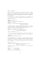
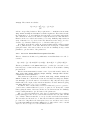
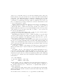
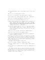
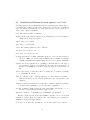
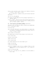
In the early stages of an analysis, where computational speed and accuracy may
be secondary considerations, the use of finite differences to compute these partial
derivatives may be very handy. Here we illustrate the same analysis using finite
differences. This is activated by replacing the named list fhn as argument by a
reference to only the right side evaluation function fn.
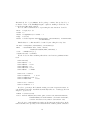
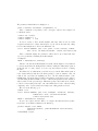
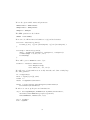
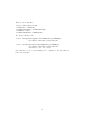
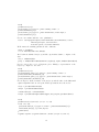
res1 = Profile.LS(fhn$fn, data, times, pars=spars, coefs=coefs,
lambda=lambda, in.meth=’nlminb’, out.meth=’nls’,
control.in=control.in, control.out=control.out)
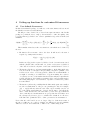
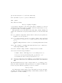
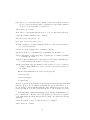
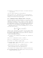
A more sophisticated choice of fitting criterion involves assuming that the noisy
data arise from a multivariate normal distribution. Function Profile.mulinorm()
implements this.
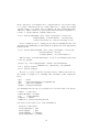
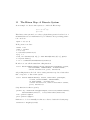
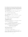
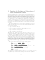
res2 = Profile.multinorm(fhn, data, times, pars=spars, coefs=coefs,
basisvals=bbasis, var=var,
in.meth=’nlminb’, out.meth=’nlminb’)
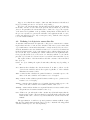
But if we want to work with lik and proc objects, we can call function LS.setup
to these up explicitly.
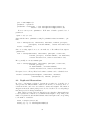
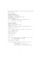
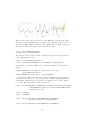
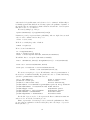
profile.obj = LS.setup(pars=pars, fn=fhn, basisvals=bbasis,
lambda=10000, times=times, fd.obj=DEfd)
lik = profile.obj$lik
proc = profile.obj$proc
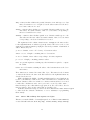
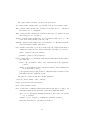
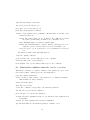
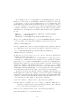
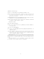
However, we can also bypass the automatic features of function profile.obj.
For example, we might need to manually define quadrature points, weights and
knots.
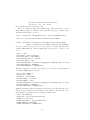
qpts
qwts
qwts
weights
=
=
=
=
knots
rep(1/length(knots),length(knots))
qwts %*% t(lambda)
array(1,dim(data))
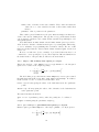
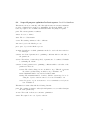
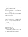
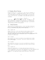
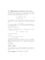
Now manually define the lik object as squared error from the values of the system:
likmore
= make.id()
likmore$weights = weights
lik
= make.SSElik()
lik$more = likmore
lik$bvals = eval.basis(times,bbasis)
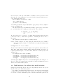
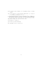
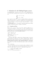
Object proc is also squared error, defined manually by
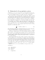
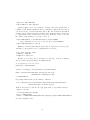
procmore = make.fhn()
procmore$weights = qwts
procmore$qpts
= qpts
procmore$names
= varnames
procmore$parnames = parnames
49