Download Scilab Interface

Scilab Interface
Release 4.0
Yves Renard, Julien Pommier
March 22, 2010
CONTENTS
1
Introduction
1
2
Installation
3
3
GetFEM++ organization
3.1 Functions . . . . . . . . . . . . . . . . . . . . . . . . . . . . . . . . . . . . . . . . . . . . . . . . .
3.2 Objects . . . . . . . . . . . . . . . . . . . . . . . . . . . . . . . . . . . . . . . . . . . . . . . . . .
5
5
7
4
Command reference
4.1 Types . . . . . . . . . .
4.2 gf_asm . . . . . . . . .
4.3 gf_compute . . . . . . .
4.4 gf_cvstruct_get . . . . .
4.5 gf_delete . . . . . . . .
4.6 gf_eltm . . . . . . . . .
4.7 gf_fem . . . . . . . . .
4.8 gf_fem_get . . . . . . .
4.9 gf_geotrans . . . . . . .
4.10 gf_geotrans_get . . . .
4.11 gf_global_function . . .
4.12 gf_global_function_get .
4.13 gf_integ . . . . . . . . .
4.14 gf_integ_get . . . . . .
4.15 gf_levelset . . . . . . .
4.16 gf_levelset_get . . . . .
4.17 gf_levelset_set . . . . .
4.18 gf_linsolve . . . . . . .
4.19 gf_mdbrick . . . . . . .
4.20 gf_mdbrick_get . . . . .
4.21 gf_mdbrick_set . . . . .
4.22 gf_mdstate . . . . . . .
4.23 gf_mdstate_get . . . . .
4.24 gf_mdstate_set . . . . .
4.25 gf_mesh . . . . . . . .
4.26 gf_mesh_get . . . . . .
4.27 gf_mesh_set . . . . . .
4.28 gf_mesh_fem . . . . . .
4.29 gf_mesh_fem_get . . .
4.30 gf_mesh_fem_set . . . .
.
.
.
.
.
.
.
.
.
.
.
.
.
.
.
.
.
.
.
.
.
.
.
.
.
.
.
.
.
.
.
.
.
.
.
.
.
.
.
.
.
.
.
.
.
.
.
.
.
.
.
.
.
.
.
.
.
.
.
.
.
.
.
.
.
.
.
.
.
.
.
.
.
.
.
.
.
.
.
.
.
.
.
.
.
.
.
.
.
.
.
.
.
.
.
.
.
.
.
.
.
.
.
.
.
.
.
.
.
.
.
.
.
.
.
.
.
.
.
.
.
.
.
.
.
.
.
.
.
.
.
.
.
.
.
.
.
.
.
.
.
.
.
.
.
.
.
.
.
.
.
.
.
.
.
.
.
.
.
.
.
.
.
.
.
.
.
.
.
.
.
.
.
.
.
.
.
.
.
.
.
.
.
.
.
.
.
.
.
.
.
.
.
.
.
.
.
.
.
.
.
.
.
.
.
.
.
.
.
.
.
.
.
.
.
.
.
.
.
.
.
.
.
.
.
.
.
.
.
.
.
.
.
.
.
.
.
.
.
.
.
.
.
.
.
.
.
.
.
.
.
.
.
.
.
.
.
.
.
.
.
.
.
.
.
.
.
.
.
.
.
.
.
.
.
.
.
.
.
.
.
.
.
.
.
.
.
.
.
.
.
.
.
.
.
.
.
.
.
.
.
.
.
.
.
.
.
.
.
.
.
.
.
.
.
.
.
.
.
.
.
.
.
.
.
.
.
.
.
.
.
.
.
.
.
.
.
.
.
.
.
.
.
.
.
.
.
.
.
.
.
.
.
.
.
.
.
.
.
.
.
.
.
.
.
.
.
.
.
.
.
.
.
.
.
.
.
.
.
.
.
.
.
.
.
.
.
.
.
.
.
.
.
.
.
.
.
.
.
.
.
.
.
.
.
.
.
.
.
.
.
.
.
.
.
.
.
.
.
.
.
.
.
.
.
.
.
.
.
.
.
.
.
.
.
.
.
.
.
.
.
.
.
.
.
.
.
.
.
.
.
.
.
.
.
.
.
.
.
.
.
.
.
.
.
.
.
.
.
.
.
.
.
.
.
.
.
.
.
.
.
.
.
.
.
.
.
.
.
.
.
.
.
.
.
.
.
.
.
.
.
.
.
.
.
.
.
.
.
.
.
.
.
.
.
.
.
.
.
.
.
.
.
.
.
.
.
.
.
.
.
.
.
.
.
.
.
.
.
.
.
.
.
.
.
.
.
.
.
.
.
.
.
.
.
.
.
.
.
.
.
.
.
.
.
.
.
.
.
.
.
.
.
.
.
.
.
.
.
.
.
.
.
.
.
.
.
.
.
.
.
.
.
.
.
.
.
.
.
.
.
.
.
.
.
.
.
.
.
.
.
.
.
.
.
.
.
.
.
.
.
.
.
.
.
.
.
.
.
.
.
.
.
.
.
.
.
.
.
.
.
.
.
.
.
.
.
.
.
.
.
.
.
.
.
.
.
.
.
.
.
.
.
.
.
.
.
.
.
.
.
.
.
.
.
.
.
.
.
.
.
.
.
.
.
.
.
.
.
.
.
.
.
.
.
.
.
.
.
.
.
.
.
.
.
.
.
.
.
.
.
.
.
.
.
.
.
.
.
.
.
.
.
.
.
.
.
.
.
.
.
.
.
.
.
.
.
.
.
.
.
.
.
.
.
.
.
.
.
.
.
.
.
.
.
.
.
.
.
.
.
.
.
.
.
.
.
.
.
.
.
.
.
.
.
.
.
.
.
.
.
.
.
.
.
.
.
.
.
.
.
.
.
.
.
.
.
.
.
.
.
.
.
.
.
.
.
.
.
.
.
.
.
.
.
.
.
.
.
.
.
.
.
.
.
.
.
.
.
.
.
.
.
.
.
.
.
.
.
.
.
.
.
.
.
.
.
.
.
.
.
.
.
.
.
.
.
.
.
.
.
.
.
.
.
.
.
.
.
.
.
.
.
.
.
.
.
.
.
.
.
.
.
.
.
.
.
.
.
.
.
.
.
.
.
.
.
.
.
.
.
.
.
.
.
.
.
.
.
.
.
.
.
.
.
.
.
.
.
.
.
.
.
.
.
.
.
.
.
.
.
.
.
.
.
.
.
.
.
.
.
.
.
.
.
.
.
.
.
.
.
.
.
.
.
.
.
.
.
.
.
.
.
.
.
.
.
.
.
.
.
.
.
.
.
.
.
.
.
.
.
.
.
.
.
.
.
.
.
.
.
.
.
.
.
.
.
.
.
.
.
.
.
.
.
.
.
.
.
.
.
.
.
.
.
.
.
.
.
.
.
.
.
.
.
.
.
.
.
.
.
.
.
.
.
.
.
.
.
.
.
.
.
.
.
.
.
.
.
.
.
.
.
.
.
.
.
.
.
.
.
.
.
.
.
.
.
.
.
.
.
.
.
.
.
.
.
.
.
.
.
.
.
.
.
.
.
.
.
.
.
.
.
.
.
.
.
.
.
.
.
.
.
.
.
.
.
.
.
.
.
.
.
.
.
.
.
.
.
.
.
.
.
.
.
.
.
.
.
.
.
.
.
.
.
.
.
.
.
.
.
.
.
.
.
.
.
.
.
.
.
.
.
.
.
.
.
.
.
.
.
.
.
.
.
.
.
.
.
.
.
.
.
.
.
.
.
.
.
.
.
.
.
.
.
.
.
.
.
.
.
.
.
.
.
.
.
.
.
.
.
.
.
.
.
.
.
.
.
.
.
.
.
.
.
.
.
.
.
.
.
.
.
.
.
.
.
.
.
.
9
9
9
13
15
16
16
17
18
20
21
22
22
23
24
25
26
26
27
28
32
34
34
35
36
37
39
43
46
47
51
i
4.31
4.32
4.33
4.34
4.35
4.36
4.37
4.38
4.39
4.40
4.41
4.42
4.43
4.44
4.45
4.46
4.47
4.48
4.49
4.50
4.51
Index
ii
gf_mesh_im . . . . .
gf_mesh_im_get . . .
gf_mesh_im_set . . .
gf_mesh_levelset . . .
gf_mesh_levelset_get
gf_mesh_levelset_set .
gf_model . . . . . . .
gf_model_get . . . . .
gf_model_set . . . . .
gf_poly . . . . . . . .
gf_precond . . . . . .
gf_precond_get . . . .
gf_slice . . . . . . . .
gf_slice_get . . . . . .
gf_slice_set . . . . . .
gf_spmat . . . . . . .
gf_spmat_get . . . . .
gf_spmat_set . . . . .
gf_undelete . . . . . .
gf_util . . . . . . . .
gf_workspace . . . . .
.
.
.
.
.
.
.
.
.
.
.
.
.
.
.
.
.
.
.
.
.
.
.
.
.
.
.
.
.
.
.
.
.
.
.
.
.
.
.
.
.
.
.
.
.
.
.
.
.
.
.
.
.
.
.
.
.
.
.
.
.
.
.
.
.
.
.
.
.
.
.
.
.
.
.
.
.
.
.
.
.
.
.
.
.
.
.
.
.
.
.
.
.
.
.
.
.
.
.
.
.
.
.
.
.
.
.
.
.
.
.
.
.
.
.
.
.
.
.
.
.
.
.
.
.
.
.
.
.
.
.
.
.
.
.
.
.
.
.
.
.
.
.
.
.
.
.
.
.
.
.
.
.
.
.
.
.
.
.
.
.
.
.
.
.
.
.
.
.
.
.
.
.
.
.
.
.
.
.
.
.
.
.
.
.
.
.
.
.
.
.
.
.
.
.
.
.
.
.
.
.
.
.
.
.
.
.
.
.
.
.
.
.
.
.
.
.
.
.
.
.
.
.
.
.
.
.
.
.
.
.
.
.
.
.
.
.
.
.
.
.
.
.
.
.
.
.
.
.
.
.
.
.
.
.
.
.
.
.
.
.
.
.
.
.
.
.
.
.
.
.
.
.
.
.
.
.
.
.
.
.
.
.
.
.
.
.
.
.
.
.
.
.
.
.
.
.
.
.
.
.
.
.
.
.
.
.
.
.
.
.
.
.
.
.
.
.
.
.
.
.
.
.
.
.
.
.
.
.
.
.
.
.
.
.
.
.
.
.
.
.
.
.
.
.
.
.
.
.
.
.
.
.
.
.
.
.
.
.
.
.
.
.
.
.
.
.
.
.
.
.
.
.
.
.
.
.
.
.
.
.
.
.
.
.
.
.
.
.
.
.
.
.
.
.
.
.
.
.
.
.
.
.
.
.
.
.
.
.
.
.
.
.
.
.
.
.
.
.
.
.
.
.
.
.
.
.
.
.
.
.
.
.
.
.
.
.
.
.
.
.
.
.
.
.
.
.
.
.
.
.
.
.
.
.
.
.
.
.
.
.
.
.
.
.
.
.
.
.
.
.
.
.
.
.
.
.
.
.
.
.
.
.
.
.
.
.
.
.
.
.
.
.
.
.
.
.
.
.
.
.
.
.
.
.
.
.
.
.
.
.
.
.
.
.
.
.
.
.
.
.
.
.
.
.
.
.
.
.
.
.
.
.
.
.
.
.
.
.
.
.
.
.
.
.
.
.
.
.
.
.
.
.
.
.
.
.
.
.
.
.
.
.
.
.
.
.
.
.
.
.
.
.
.
.
.
.
.
.
.
.
.
.
.
.
.
.
.
.
.
.
.
.
.
.
.
.
.
.
.
.
.
.
.
.
.
.
.
.
.
.
.
.
.
.
.
.
.
.
.
.
.
.
.
.
.
.
.
.
.
.
.
.
.
.
.
.
.
.
.
.
.
.
.
.
.
.
.
.
.
.
.
.
.
.
.
.
.
.
.
.
.
.
.
.
.
.
.
.
.
.
.
.
.
.
.
.
.
.
.
.
.
.
.
.
.
.
.
.
.
.
.
.
.
.
.
.
.
.
.
.
.
.
.
.
.
.
.
.
.
.
.
.
.
.
.
.
.
.
.
.
.
.
.
.
.
.
.
.
.
.
.
.
.
.
.
.
.
.
.
.
.
.
.
.
.
.
.
.
.
.
.
.
.
.
.
.
.
.
.
.
.
.
.
.
.
.
.
.
.
.
.
.
.
.
.
.
.
.
.
.
.
.
.
.
.
.
.
.
.
.
.
.
.
.
.
.
.
.
.
.
.
.
.
.
.
.
.
.
.
.
.
.
.
.
.
.
.
.
.
.
.
.
.
.
.
.
.
.
.
.
.
.
.
.
.
.
.
.
.
.
.
.
.
.
.
.
.
.
.
.
.
.
.
.
.
.
.
.
.
.
.
.
.
.
.
.
.
.
.
.
.
.
.
.
.
.
.
.
.
.
.
52
53
54
55
55
56
57
57
59
68
68
69
70
73
75
75
77
78
80
80
81
83
CHAPTER
ONE
INTRODUCTION
This guide provides a reference about the SciLab interface of GetFEM++. For a complete reference of GetFEM++,
please report to the specific guides, but you should be able to use the scilab interface without any particular knowledge
of the GetFEM++ internals, although a basic knowledge about Finite Elements is required.
Copyright © 2000-2010 Yves Renard, Julien Pommier.
The text of the GetFEM++ website and the documentations are available for modification and reuse under the terms
of the GNU Free Documentation License
The program GetFEM++ is free software; you can redistribute it and/or modify it under the terms of the GNU Lesser
General Public License as published by the Free Software Foundation; version 2.1 of the License. This program is
distributed in the hope that it will be useful, but WITHOUT ANY WARRANTY; without even the implied warranty of
MERCHANTABILITY or FITNESS FOR A PARTICULAR PURPOSE. See the GNU Lesser General Public License
for more details. You should have received a copy of the GNU Lesser General Public License along with this program;
if not, write to the Free Software Foundation, Inc., 59 Temple Place - Suite 330, Boston, MA 02111-1307, USA.
1
Scilab Interface, Release 4.0
2
Chapter 1. Introduction
CHAPTER
TWO
INSTALLATION
The installation of the getfem-interface toolbox can be somewhat tricky, since it combines a C++ compiler, libraries
and SciLab interaction... In case of troubles with a non-GNU compiler, gcc/g++ (>= 4.1) should be a safe solution.
Caution:
• you should not use a different compiler than the one that was used for the GetFEM++ library.
• you should have built the GetFEM++ static library (i.e. do not use ./configure -disable-static
when building GetFEM++). On linux/x86_64 platforms, a mandatory option when building GetFEM++ and getfem-interface (and any static library linked to them) is the -with-pic option of their
./configure script.
• you should have use the –enable-scilab option to configure the GetFEM++ sources (i.e. ./configure –enablematlab ...)
You may also use -with-toolbox-dir=toolbox_dir to change the default toolbox installation directory
(gfdest_dir/getfem_toolbox). Use ./configure -help for more options.
With this, since the Scilab interface is contained into the GetFEM++ sources (in the directory interface/src) you can
compile both the GetFEM++ library and the Scilab interface by
make
An optional step is make check in order to check the scilab interface ... and install it ( ... ):
make install
If you want to use a different compiler than the one chosen automatically by the ./configure script, just specify
its name on the command line: ./configure CXX=mycompiler.
When the library is installed,
completer les instructions ...
...
A very classical problem at this step is the incompatibility of the C and C++ libraries used by Scilab. Scilab is
distributed with its own libc and libstdc++ libraries. An error message of the following type occurs when one tries to
use a command of the interface:
/usr/local/matlab14-SP3/bin/glnxa64/../../sys/os/??/libgcc_s.so.1:
version ‘GCC_?.?’ not found (required by .../gf_matlab.mex??).
3
Scilab Interface, Release 4.0
In order to fix this problem one has to enforce Scilab to load the C and C++ libraries of the system. There is two
possibilities to do this. The most radical is to delete the C and C++ libraries distributed along with Matlab (if you have
administrator privileges ...!) for instance with:
rm ‘a completer‘/libgcc_s.so.1
rm ‘a completer‘/libstdc++_s.so.6
The second possibility is to set the variable LDPRELOAD before launching Matlab for instance with (depending on
the system):
LD_PRELOAD=/usr/lib/libgcc_s.so:/usr/lib/libstdc++.so.6 scilab
More specific instructions can be found in the README* files of the distribution.
4
Chapter 2. Installation
CHAPTER
THREE
GETFEM++ ORGANIZATION
The GetFEM++ toolbox is just a convenient interface to the GetFEM++ library: you must have a working GetFEM++
installed on your computer. All the functions of GetFEM++ are prefixed by gf_ (hence typing gf_ at the SciLab
prompt and then pressing the <tab> key is a quick way to obtain the list of getfem functions).
3.1 Functions
• gf_workspace : workspace management.
• gf_util : miscellanous utility functions.
• gf_delete : destroy a GetFEM++ object (gfMesh , gfMeshFem , gfMeshIm etc.).
• gf_cvstruct_get : retrieve informations from a gfCvStruct object.
• gf_geotrans : define a geometric transformation.
• gf_geotrans_get : retrieve informations from a gfGeoTrans object.
• gf_mesh : creates a new gfMesh object.
• gf_mesh_get : retrieve informations from a gfMesh object.
• gf_mesh_set : modify a gfMesh object.
• gf_eltm : define an elementary matrix.
• gf_fem : define a gfFem.
• gf_fem_get : retrieve informations from a gfFem object.
• gf_integ : define a integration method.
• gf_integ_get : retrieve informations from an gfInteg object.
• gf_mesh_fem : creates a new gfMeshFem object.
• gf_mesh_fem_get : retrieve informations from a gfMeshFem object.
• gf_mesh_fem_set : modify a gfMeshFem object.
• gf_mesh_im : creates a new gfMeshIm object.
• gf_mesh_im_get : retrieve informations from a gfMeshIm object.
• gf_mesh_im_set : modify a gfMeshIm object.
5
Scilab Interface, Release 4.0
• gf_slice : create a new gfSlice object.
• gf_slice_get : retrieve informations from a gfSlice object.
• gf_slice_set : modify a gfSlice object.
• gf_spmat : create a gfSpMat object.
• gf_spmat_get : perform computations with the gfSpMat.
• gf_spmat_set : modify the gfSpMat.
• gf_precond : create a gfPrecond object.
• gf_precond_get : perform computations with the gfPrecond.
• gf_linsolve : interface to various linear solvers provided by getfem (SuperLU, conjugated gradient, etc.).
• gf_asm : assembly routines.
• gf_solve : various solvers for usual PDEs (obsoleted by the gfMdBrick objects).
• gf_compute : computations involving the solution of a PDE (norm, derivative, etc.).
• gf_mdbrick : create a (“model brick”) gfMdBrick object.
• gf_mdbrick_get : retrieve information from a gfMdBrick object.
• gf_mdbrick_set : modify a gfMdBrick object.
• gf_mdstate : create a (“model state”) gfMdState object.
• gf_mdstate_get : retrieve information from a gfMdState object.
• gf_mdstate_set : modify a gfMdState object.
• gf_model : create a gfModel object.
• gf_model_get : retrieve information from a gfModel object.
• gf_model_set : modify a gfModel object.
• gf_global_function : create a gfGlobalFunction object.
• gf_model_get : retrieve information from a gfGlobalFunction object.
• gf_model_set : modify a GlobalFunction object.
• gf_plot_mesh : plotting of mesh.
• gf_plot : plotting of 2D and 3D fields.
• gf_plot_1D : plotting of 1D fields.
• gf_plot_slice : plotting of a mesh slice.
6
Chapter 3. GetFEM++ organization
Scilab Interface, Release 4.0
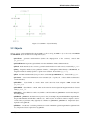
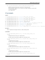
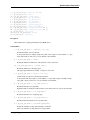
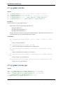
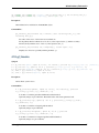
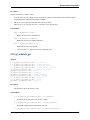
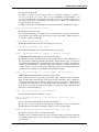
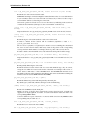
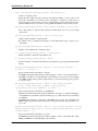
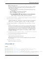
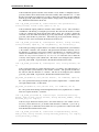
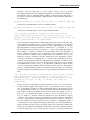
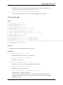
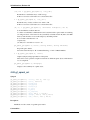
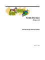
Figure 3.1: GetFEM++ objects hierarchy.
3.2 Objects
Various “objects” can be manipulated by the GetFEM++ toolbox, see fig. GetFEM++ objects hierarchy.. The MESH
and MESHFEM objects are the two most important objects.
• gfGeoTrans: geometric transformations (defines the shape/position of the convexes), created with
gf_geotrans
• gfGlobalFunction: represent a global function for the enrichment of finite element methods.
• gfMesh : mesh structure (nodes, convexes, geometric transformations for each convex), created with gf_mesh
• gfInteg : integration method (exact, quadrature formula...). Although not linked directly to GEOTRANS, an
integration method is usually specific to a given convex structure. Created with gf_integ
• gfFem : the finite element method (one per convex, can be PK, QK, HERMITE, etc.). Created with gf_fem
• gfCvStruct : stores formal information convex structures (nb. of points, nb. of faces which are themselves
convex structures).
• gfMeshFem : object linked to a mesh, where each convex has been assigned a FEM. Created with
gf_mesh_fem.
• gfMeshImM : object linked to a mesh, where each convex has been assigned an integration method. Created
with gf_mesh_im.
• gfMeshSlice : object linked to a mesh, very similar to a P1-discontinuous gfMeshFem. Used for fast interpolation and plotting.
• gfMdBrick : gfMdBrick , an abstraction of a part of solver (for example, the part which build the tangent matrix,
the part which handles the dirichlet conditions, etc.). These objects are stacked to build a complete solver for
a wide variety of problems. They typically use a number of gfMeshFem, gfMeshIm etc. Deprecated object,
replaced now by gfModel.
• gfMdState : “model state”, holds the global data for a stack of mdbricks (global tangent matrix, right hand side
etc.). Deprecated object, replaced now by gfModel.
3.2. Objects
7
Scilab Interface, Release 4.0
• gfModel : “model”, holds the global data, variables and description of a model. Evolution of “model state”
object for 4.0 version of GetFEM++.
The GetFEM++ toolbox uses its own memory management. Hence GetFEM++ objects are not cleared when a:
>> clear all
is issued at the SciLab prompt, but instead the function:
>> gf_workspace(’clear all’)
should be used. The various GetFEM++ object can be accessed via handles (or descriptors), which are just SciLab
structures containing 32-bits integer identifiers to the real objects. Hence the SciLab command:
>> whos
does not report the memory consumption of GetFEM++ objects (except the marginal space used by the handle).
Instead, you should use:
>> gf_workspace(’stats’)
There are two kinds of GetFEM++ objects:
• static ones, which can not be deleted: ELTM, FEM, INTEG, GEOTRANS and CVSTRUCT. Hopefully their
memory consumption is very low.
• dynamic ones, which can be destroyed, and are handled by the gf_workspace function: MESH, MESHFEM,
MESHIM, SLICE, SPMAT, PRECOND.
The objects MESH and MESHFEM are not independent: a MESHFEM object is always linked to a MESH object,
and a MESH object can be used by several MESHFEM objects. Hence when you request the destruction of a MESH
object, its destruction might be delayed until it is not used anymore by any MESHFEM (these objects waiting for
deletion are listed in the anonymous workspace section of gf_workspace(’stats’)).
8
Chapter 3. GetFEM++ organization
CHAPTER
FOUR
COMMAND REFERENCE
4.1 Types
The expected type of each function argument is indicated in this reference. Here is a list of these types:
int
hobj
scalar
string
ivec
vec
imat
mat
spmat
precond
mesh mesh
mesh_fem
mesh_im
mesh_slice
cvstruct
geotrans
fem
eltm
integ
model
global_function
integer value
a handle for any getfem++ object
scalar value
string
vector of integer values
vector
matrix of integer values
matrix
sparse matrix (both matlab native sparse matrices, and getfem sparse matrices)
getfem preconditioner object
object descriptor (or gfMesh object)
mesh fem object descriptor (or gfMeshFem object)
mesh im object descriptor( or gfMeshIm object)
mesh slice object descriptor (or gfSlice object)
convex structure descriptor (or gfCvStruct object)
geometric transformation descriptor (or gfGeoTrans object)
fem descriptor (or gfFem object)
elementary matrix descriptor (or gfEltm object)
integration method descriptor (or gfInteg object)
model descriptor (or gfModel object)
global function descriptor
Arguments listed between square brackets are optional. Lists between braces indicate that the argument must match
one of the elements of the list. For example:
>> [X,Y]=dummy(int i, ’foo’ | ’bar’ [,vec v])
means that the dummy function takes two or three arguments, its first being an integer value, the second a string which
is either ‘foo’ or ‘bar’, and a third optional argument. It returns two values (with the usual matlab meaning, i.e. the
caller can always choose to ignore them).
4.2 gf_asm
Synopsis
9
Scilab Interface, Release 4.0
M = gf_asm(’mass matrix’, mesh_im mim, mesh_fem mf1[, mesh_fem mf2])
L = gf_asm(’laplacian’, mesh_im mim, mesh_fem mf_u, mesh_fem mf_d, vec a)
Le = gf_asm(’linear elasticity’, mesh_im mim, mesh_fem mf_u, mesh_fem mf_d, vec lambda_d, vec mu_d)
TRHS = gf_asm(’nonlinear elasticity’, mesh_im mim, mesh_fem mf_u, vec U, string law, mesh_fem mf_d, m
{K, B} = gf_asm(’stokes’, mesh_im mim, mesh_fem mf_u, mesh_fem mf_p, mesh_fem mf_d, vec nu)
A = gf_asm(’helmholtz’, mesh_im mim, mesh_fem mf_u, mesh_fem mf_d, vec k)
A = gf_asm(’bilaplacian’, mesh_im mim, mesh_fem mf_u, mesh_fem mf_d, vec a)
V = gf_asm(’volumic source’, mesh_im mim, mesh_fem mf_u, mesh_fem mf_d, vec fd)
B = gf_asm(’boundary source’, int bnum, mesh_im mim, mesh_fem mf_u, mesh_fem mf_d, vec G)
{HH, RR} = gf_asm(’dirichlet’, int bnum, mesh_im mim, mesh_fem mf_u, mesh_fem mf_d, mat H, vec R [, t
Q = gf_asm(’boundary qu term’,int boundary_num, mesh_im mim, mesh_fem mf_u, mesh_fem mf_d, mat q)
{...} = gf_asm(’volumic’ [,CVLST], expr [, mesh_ims, mesh_fems, data...])
{...} = gf_asm(’boundary’, int bnum, string expr [, mesh_im mim, mesh_fem mf, data...])
Mi = gf_asm(’interpolation matrix’, mesh_fem mf, mesh_fem mfi)
Me = gf_asm(’extrapolation matrix’,mesh_fem mf, mesh_fem mfe)
Description :
General assembly function.
Many of the functions below use more than one mesh_fem: the main mesh_fem (mf_u) used for the main
unknow, and data mesh_fem (mf_d) used for the data. It is always assumed that the Qdim of mf_d is
equal to 1: if mf_d is used to describe vector or tensor data, you just have to “stack” (in fortran ordering)
as many scalar fields as necessary.
Command list :
M = gf_asm(’mass matrix’, mesh_im mim, mesh_fem mf1[, mesh_fem mf2])
Assembly of a mass matrix.
Return a spmat object.
L = gf_asm(’laplacian’, mesh_im mim, mesh_fem mf_u, mesh_fem mf_d,
vec a)
Assembly of the matrix for the Laplacian problem.
∇ · (a(x)∇u) with a a scalar.
Return a spmat object.
Le = gf_asm(’linear elasticity’, mesh_im mim, mesh_fem mf_u, mesh_fem
mf_d, vec lambda_d, vec mu_d)
Assembles of the matrix for the linear (isotropic) elasticity problem.
∇ · (C(x) : ∇u) with C defined via lambda_d and mu_d.
Return a spmat object.
TRHS = gf_asm(’nonlinear elasticity’, mesh_im mim, mesh_fem
mf_u, vec U, string law, mesh_fem mf_d, mat params, {’tangent
matrix’|’rhs’|’incompressible tangent matrix’, mesh_fem mf_p, vec
P|’incompressible rhs’, mesh_fem mf_p, vec P})
Assembles terms (tangent matrix and right hand side) for nonlinear elasticity.
The solution U is required at the current time-step. The law may be choosen among:
• ‘SaintVenant Kirchhoff’: Linearized law, should be avoided). This law has the two usual
Lame coefficients as parameters, called lambda and mu.
10
Chapter 4. Command reference
Scilab Interface, Release 4.0
• ‘Mooney Rivlin’: Only for incompressibility. This law has two parameters, called C1 and
C2.
• ‘Ciarlet Geymonat’: This law has 3 parameters, called lambda, mu and gamma, with
gamma chosen such that gamma is in ]-lambda/2-mu, -mu[.
The parameters of the material law are described on the mesh_fem mf_d. The matrix params
should have nbdof(mf_d) columns, each row correspounds to a parameter.
The last argument selects what is to be built: either the tangent matrix, or the right hand side.
If the incompressibility is considered, it should be followed by a mesh_fem mf_p, for the
pression.
Return a spmat object (tangent matrix), vec object (right hand side), tuple of spmat objects
(incompressible tangent matrix), or tuple of vec objects (incompressible right hand side).
{K, B} = gf_asm(’stokes’, mesh_im mim, mesh_fem mf_u, mesh_fem mf_p,
mesh_fem mf_d, vec nu)
Assembly of matrices for the Stokes problem.
−ν(x)∆u + ∇p = 0 ∇ · u = 0 with ν (nu), the fluid’s dynamic viscosity.
On output, K is the
R usual linear elasticity stiffness matrix with λ = 0 and 2µ = ν. B is a matrix
corresponding to p∇ · φ.
K and B are spmat object’s.
A = gf_asm(’helmholtz’, mesh_im mim, mesh_fem mf_u, mesh_fem mf_d,
vec k)
Assembly of the matrix for the Helmholtz problem.
∆u + k 2 u = 0, with k complex scalar.
Return a spmat object.
A = gf_asm(’bilaplacian’, mesh_im mim, mesh_fem mf_u, mesh_fem mf_d,
vec a)
Assembly of the matrix for the Bilaplacian problem.
∆(a(x)∆u) = 0 with a scalar.
Return a spmat object.
V = gf_asm(’volumic source’, mesh_im mim, mesh_fem mf_u, mesh_fem
mf_d, vec fd)
Assembly of a volumic source term.
Output a vector V, assembled on the mesh_fem mf_u, using the data vector fd defined on the
data mesh_fem mf_d. fd may be real or complex-valued.
Return a vec object.
B = gf_asm(’boundary source’, int bnum, mesh_im mim, mesh_fem mf_u,
mesh_fem mf_d, vec G)
Assembly of a boundary source term.
G should be a [Qdim x N] matrix, where N is the number of dof of mf_d, and Qdim is the
dimension of the unkown u (that is set when creating the mesh_fem).
Return a vec object.
{HH, RR} = gf_asm(’dirichlet’, int bnum, mesh_im mim, mesh_fem mf_u,
mesh_fem mf_d, mat H, vec R [, threshold])
4.2. gf_asm
11
Scilab Interface, Release 4.0
Assembly of Dirichlet conditions of type h.u = r.
Handle h.u = r where h is a square matrix (of any rank) whose size is equal to the dimension of
the unkown u. This matrix is stored in H, one column per dof in mf_d, each column containing
the values of the matrix h stored in fortran order:
‘H(:, j) = [h11(xj )h21(xj )h12(xj )h22(xj )]‘
if u is a 2D vector field.
Of course, if the unknown is a scalar field, you just have to set H = ones(1, N), where N is the
number of dof of mf_d.
This is basically the same than calling gf_asm(‘boundary qu term’) for H and calling
gf_asm(‘neumann’) for R, except that this function tries to produce a ‘better’ (more diagonal) constraints matrix (when possible).
See also gf_spmat_get(spmat S, ‘Dirichlet_nullspace’).
Q = gf_asm(’boundary qu term’,int boundary_num, mesh_im mim, mesh_fem
mf_u, mesh_fem mf_d, mat q)
Assembly of a boundary qu term.
q should be be a [Qdim x Qdim x N] array, where N is the number of dof of mf_d, and Qdim
is the dimension of the unkown u (that is set when creating the mesh_fem).
Return a spmat object.
{...} = gf_asm(’volumic’ [,CVLST], expr [, mesh_ims, mesh_fems,
data...])
Generic assembly procedure for volumic assembly.
The expression expr is evaluated over the mesh_fem’s listed in the arguments (with optional
data) and assigned to the output arguments. For details about the syntax of assembly expressions, please refer to the getfem user manual (or look at the file getfem_assembling.h in the
getfem++ sources).
For example, the L2 norm of a field can be computed with:
gf_compute(’L2 norm’) or with:
gf_asm(’volumic’,’u=data(#1); V()+=u(i).u(j).comp(Base(#1).Base(#1))(i,j)’,mim,mf,U)
The Laplacian stiffness matrix can be evaluated with:
gf_asm(’laplacian’,mim, mf, A) or equivalently with:
gf_asm(’volumic’,’a=data(#2);M(#1,#1)+=sym(comp(Grad(#1).Grad(#1).Base(#2))(:,i,:,i,j).a(j))
{...} = gf_asm(’boundary’, int bnum, string expr [, mesh_im mim,
mesh_fem mf, data...])
Generic boundary assembly.
See the help for gf_asm(‘volumic’).
Mi = gf_asm(’interpolation matrix’, mesh_fem mf, mesh_fem mfi)
Build the interpolation matrix from a mesh_fem onto another mesh_fem.
Return a matrix Mi, such that V = Mi.U is equal to gf_compute(‘interpolate_on’,mfi). Useful
for repeated interpolations. Note that this is just interpolation, no elementary integrations are
involved here, and mfi has to be lagrangian. In the more general case, you would have to do a
L2 projection via the mass matrix.
Mi is a spmat object.
12
Chapter 4. Command reference
Scilab Interface, Release 4.0
Me = gf_asm(’extrapolation matrix’,mesh_fem mf, mesh_fem mfe)
Build the extrapolation matrix from a mesh_fem onto another mesh_fem.
Return a matrix Me, such that V = Me.U is equal to gf_compute(‘extrapolate_on’,mfe). Useful
for repeated extrapolations.
Me is a spmat object.
4.3 gf_compute
Synopsis
n = gf_compute(mesh_fem MF, vec U, ’L2 norm’, mesh_im mim[, mat CVids])
n = gf_compute(mesh_fem MF, vec U, ’H1 semi norm’, mesh_im mim[, mat CVids])
n = gf_compute(mesh_fem MF, vec U, ’H1 norm’, mesh_im mim[, mat CVids])
n = gf_compute(mesh_fem MF, vec U, ’H2 semi norm’, mesh_im mim[, mat CVids])
n = gf_compute(mesh_fem MF, vec U, ’H2 norm’, mesh_im mim[, mat CVids])
DU = gf_compute(mesh_fem MF, vec U, ’gradient’, mesh_fem mf_du)
HU = gf_compute(mesh_fem MF, vec U, ’hessian’, mesh_fem mf_h)
UP = gf_compute(mesh_fem MF, vec U, ’eval on triangulated surface’, int Nrefine, [vec CVLIST])
Ui = gf_compute(mesh_fem MF, vec U, ’interpolate on’, {mesh_fem mfi | slice sli})
Ue = gf_compute(mesh_fem MF, vec U, ’extrapolate on’, mesh_fem mfe)
E = gf_compute(mesh_fem MF, vec U, ’error estimate’, mesh_im mim)
E = gf_compute(mesh_fem MF, vec U, ’convect’, mesh_fem mf_v, vec V, scalar dt, int nt[, string option
Description :
Various computations involving the solution U to a finite element problem.
Command list :
n = gf_compute(mesh_fem MF, vec U, ’L2 norm’, mesh_im mim[, mat
CVids])
Compute the L2 norm of the (real or complex) field U.
If CVids is given, the norm will be computed only on the listed convexes.
n = gf_compute(mesh_fem MF, vec U, ’H1 semi norm’, mesh_im mim[, mat
CVids])
Compute the L2 norm of grad(U).
If CVids is given, the norm will be computed only on the listed convexes.
n = gf_compute(mesh_fem MF, vec U, ’H1 norm’, mesh_im mim[, mat
CVids])
Compute the H1 norm of U.
If CVids is given, the norm will be computed only on the listed convexes.
n = gf_compute(mesh_fem MF, vec U, ’H2 semi norm’, mesh_im mim[, mat
CVids])
Compute the L2 norm of D^2(U).
If CVids is given, the norm will be computed only on the listed convexes.
n = gf_compute(mesh_fem MF, vec U, ’H2 norm’, mesh_im mim[, mat
CVids])
4.3. gf_compute
13
Scilab Interface, Release 4.0
Compute the H2 norm of U.
If CVids is given, the norm will be computed only on the listed convexes.
DU = gf_compute(mesh_fem MF, vec U, ’gradient’, mesh_fem mf_du)
Compute the gradient of the field U defined on mesh_fem mf_du.
The gradient is interpolated on the mesh_fem mf_du, and returned in DU. For example, if U is
defined on a P2 mesh_fem, DU should be evaluated on a P1-discontinuous mesh_fem. mf and
mf_du should share the same mesh.
U may have any number of dimensions (i.e. this function is not restricted to the gradient of
scalar fields, but may also be used for tensor fields). However the last dimension of U has to
be equal to the number of dof of mf. For example, if U is a [3x3xNmf] array (where Nmf is the
number of dof of mf ), DU will be a [Nx3x3[xQ]xNmf_du] array, where N is the dimension of
the mesh, Nmf_du is the number of dof of mf_du, and the optional Q dimension is inserted if
Qdim_mf != Qdim_mf_du, where Qdim_mf is the Qdim of mf and Qdim_mf_du is the Qdim
of mf_du.
HU = gf_compute(mesh_fem MF, vec U, ’hessian’, mesh_fem mf_h)
Compute the hessian of the field U defined on mesh_fem mf_h.
See also gf_compute(‘gradient’, mesh_fem mf_du).
UP = gf_compute(mesh_fem MF, vec U, ’eval on triangulated surface’,
int Nrefine, [vec CVLIST])
[OBSOLETE FUNCTION! will be removed in a future release] Utility function designed for
2D triangular meshes : returns a list of triangles coordinates with interpolated U values. This
can be used for the accurate visualization of data defined on a discontinous high order element.
On output, the six first rows of UP contains the triangle coordinates, and the others rows
contain the interpolated values of U (one for each triangle vertex) CVLIST may indicate the
list of convex number that should be consider, if not used then all the mesh convexes will be
used. U should be a row vector.
Ui = gf_compute(mesh_fem MF, vec U, ’interpolate on’, {mesh_fem mfi |
slice sli})
Interpolate a field on another mesh_fem or a slice.
• Interpolation on another mesh_fem mfi: mfi has to be Lagrangian. If mf and mfi share
the same mesh object, the interpolation will be much faster.
• Interpolation on a slice sli: this is similar to interpolation on a refined P1-discontinuous
mesh, but it is much faster. This can also be used with gf_slice(‘points’) to obtain
field values at a given set of points.
See also gf_asm(‘interpolation matrix’)
Ue = gf_compute(mesh_fem MF, vec U, ’extrapolate on’, mesh_fem mfe)
Extrapolate a field on another mesh_fem.
If the mesh of mfe is stricly included in the mesh of mf, this function does stricly the same job
as gf_compute(‘interpolate_on’). However, if the mesh of mfe is not exactly included in mf
(imagine interpolation between a curved refined mesh and a coarse mesh), then values which
are outside mf will be extrapolated.
See also gf_asm(‘extrapolation matrix’)
E = gf_compute(mesh_fem MF, vec U, ’error estimate’, mesh_im mim)
14
Chapter 4. Command reference
Scilab Interface, Release 4.0
Compute an a posteriori error estimate.
Currently there is only one which is available: for each convex, the jump of the normal derivative is integrated on its faces.
E = gf_compute(mesh_fem MF, vec U, ’convect’, mesh_fem mf_v, vec V,
scalar dt, int nt[, string option])
Compute a convection of U with regards to a steady state velocity field V with a CharacteristicGalerkin method. This method is restricted to pure Lagrange fems for U. mf_v should represent
a continuous finite element method. dt is the integration time and nt is the number of integration
step on the caracteristics. option is an option for the part of the boundary where there is a reentrant convection. option = ‘extrapolation’ for an extrapolation on the nearest element or
option = ‘unchanged’ for a constant value on that boundary. This method is rather dissipative,
but stable.
4.4 gf_cvstruct_get
Synopsis
n = gf_cvstruct_get(cvstruct CVS, ’nbpts’)
d = gf_cvstruct_get(cvstruct CVS, ’dim’)
cs = gf_cvstruct_get(cvstruct CVS, ’basic structure’)
cs = gf_cvstruct_get(cvstruct CVS, ’face’, int F)
I = gf_cvstruct_get(cvstruct CVS, ’facepts’, int F)
s = gf_cvstruct_get(cvstruct CVS, ’char’)
gf_cvstruct_get(cvstruct CVS, ’display’)
Description :
General function for querying information about convex_structure objects.
The convex structures are internal structures of getfem++. They do not contain points positions. These
structures are recursive, since the faces of a convex structures are convex structures.
Command list :
n = gf_cvstruct_get(cvstruct CVS, ’nbpts’)
Get the number of points of the convex structure.
d = gf_cvstruct_get(cvstruct CVS, ’dim’)
Get the dimension of the convex structure.
cs = gf_cvstruct_get(cvstruct CVS, ’basic structure’)
Get the simplest convex structure.
For example, the ‘basic structure’ of the 6-node triangle, is the canonical 3-noded triangle.
cs = gf_cvstruct_get(cvstruct CVS, ’face’, int F)
Return the convex structure of the face F.
I = gf_cvstruct_get(cvstruct CVS, ’facepts’, int F)
Return the list of point indices for the face F.
4.4. gf_cvstruct_get
15
Scilab Interface, Release 4.0
s = gf_cvstruct_get(cvstruct CVS, ’char’)
Output a string description of the cvstruct.
gf_cvstruct_get(cvstruct CVS, ’display’)
displays a short summary for a cvstruct object.
4.5 gf_delete
Synopsis
gf_delete(I[, J, K,...])
Description :
Delete an existing getfem object from memory (mesh, mesh_fem, etc.).
SEE ALSO: gf_workspace, gf_mesh, gf_mesh_fem.
Command list :
gf_delete(I[, J, K,...])
I should be a descriptor given by gf_mesh(), gf_mesh_im(), gf_slice() etc.
Note that if another object uses I, then object I will be deleted only when both have been asked
for deletion.
Only objects listed in the output of gf_workspace(‘stats’) can be deleted (for example gf_fem
objects cannot be destroyed).
You may also use gf_workspace(‘clear all’) to erase everything at once.
4.6 gf_eltm
Synopsis
E
E
E
E
E
E
E
=
=
=
=
=
=
=
gf_eltm(’base’, fem FEM)
gf_eltm(’grad’, fem FEM)
gf_eltm(’hessian’, fem FEM)
gf_eltm(’normal’)
gf_eltm(’grad_geotrans’)
gf_eltm(’grad_geotrans_inv’)
gf_eltm(’product’, eltm A, eltm B)
Description :
General constructor for eltm objects.
This object represents a type of elementary matrix. In order to obtain a numerical value of theses matrices,
see gf_mesh_im_get(mesh_im MI, ‘eltm’).
If you have very particular assembling needs, or if you just want to check the content of an elementary
matrix, this function might be useful. But the generic assembly abilities of gf_asm(...) should suit most
needs.
16
Chapter 4. Command reference
Scilab Interface, Release 4.0
Command list :
E = gf_eltm(’base’, fem FEM)
return a descriptor for the integration of shape functions on elements, using the fem FEM.
E = gf_eltm(’grad’, fem FEM)
return a descriptor for the integration of the gradient of shape functions on elements, using the
fem FEM.
E = gf_eltm(’hessian’, fem FEM)
return a descriptor for the integration of the hessian of shape functions on elements, using the
fem FEM.
E = gf_eltm(’normal’)
return a descriptor for the unit normal of convex faces.
E = gf_eltm(’grad_geotrans’)
return a descriptor to the gradient matrix of the geometric transformation.
E = gf_eltm(’grad_geotrans_inv’)
return a descriptor to the inverse of the gradient matrix of the geometric transformation (this is
rarely used).
E = gf_eltm(’product’, eltm A, eltm B)
return a descriptor for the integration of the tensorial product of elementary matrices A and B.
4.7 gf_fem
Synopsis
fem TF = gf_fem(’interpolated_fem’, mesh_fem mf, mesh_im mim, [ivec blocked_dof])
gf_fem(string fem_name)
Description :
General constructor for fem objects.
This object represents a finite element method on a reference element.
Command list :
fem TF = gf_fem(’interpolated_fem’, mesh_fem mf, mesh_im mim, [ivec
blocked_dof])
Build a special fem which is interpolated from another mesh_fem.
Using this special finite element, it is possible to interpolate a given mesh_fem mf on another
mesh, given the integration method mim that will be used on this mesh.
Note that this finite element may be quite slow, and eats much memory.
gf_fem(string fem_name)
4.7. gf_fem
17
Scilab Interface, Release 4.0
The fem_name should contain a description of the finite element method. Please refer to the
getfem++ manual (especially the description of finite element and integration methods) for a
complete reference. Here is a list of some of them:
• FEM_PK(n,k) classical Lagrange element Pk on a simplex of dimension n.
• FEM_PK_DISCONTINUOUS(N,K[,alpha]) discontinuous Lagrange element Pk on a
simplex of dimension n.
• FEM_QK(n,k) classical Lagrange element Qk on quadrangles, hexahedrons etc.
• FEM_QK_DISCONTINUOUS(n,k[,alpha]) discontinuous Lagrange element Qk on
quadrangles, hexahedrons etc.
• FEM_Q2_INCOMPLETE incomplete 2D Q2 element with 8 dof (serendipity Quad 8
element).
• FEM_PK_PRISM(n,k) classical Lagrange element Pk on a prism.
• FEM_PK_PRISM_DISCONTINUOUS(n,k[,alpha]) classical discontinuous Lagrange element Pk on a prism.
• FEM_PK_WITH_CUBIC_BUBBLE(n,k) classical Lagrange element Pk on a simplex
with an additional volumic bubble function.
• FEM_P1_NONCONFORMING non-conforming P1 method on a triangle.
• FEM_P1_BUBBLE_FACE(n) P1 method on a simplex with an additional bubble function
on face 0.
• FEM_P1_BUBBLE_FACE_LAG P1 method on a simplex with an additional lagrange dof
on face 0.
• FEM_PK_HIERARCHICAL(n,k) PK element with a hierarchical basis.
• FEM_QK_HIERARCHICAL(n,k) QK element with a hierarchical basis
• FEM_PK_PRISM_HIERARCHICAL(n,k) PK element on a prism with a hierarchical basis.
• FEM_STRUCTURED_COMPOSITE(FEM,k) Composite fem on a grid with k divisions.
• FEM_PK_HIERARCHICAL_COMPOSITE(n,k,s) Pk composite element on a grid with
s subdivisions and with a hierarchical basis.
• FEM_PK_FULL_HIERARCHICAL_COMPOSITE(n,k,s) Pk composite element with s
subdivisions and a hierarchical basis on both degree and subdivision.
• FEM_PRODUCT(FEM1,FEM2) tensorial product of two polynomial elements.
• FEM_HERMITE(n) Hermite element P3 on a simplex of dimension n = 1, 2, 3.
• FEM_ARGYRIS Argyris element P5 on the triangle.
• FEM_HCT_TRIANGLE Hsieh-Clough-Tocher element on the triangle (composite P3 element which is C^1), should be used with IM_HCT_COMPOSITE() integration method.
• FEM_QUADC1_COMPOSITE Quadrilateral element, composite P3 element and C^1 (16
dof).
• FEM_REDUCED_QUADC1_COMPOSITE Quadrilateral element, composite P3 element and C^1 (12 dof).
• FEM_RT0(n) Raviart-Thomas element of order 0 on a simplex of dimension n.
• FEM_NEDELEC(n) Nedelec edge element of order 0 on a simplex of dimension n.
Of course, you have to ensure that the selected fem is compatible with the geometric transformation: a Pk fem has no meaning on a quadrangle.
4.8 gf_fem_get
Synopsis
18
Chapter 4. Command reference
Scilab Interface, Release 4.0
n = gf_fem_get(fem F, ’nbdof’[, int cv])
d = gf_fem_get(fem F, ’dim’)
td = gf_fem_get(fem F, ’target_dim’)
P = gf_fem_get(fem F, ’pts’[, int cv])
b = gf_fem_get(fem F, ’is_equivalent’)
b = gf_fem_get(fem F, ’is_lagrange’)
b = gf_fem_get(fem F, ’is_polynomial’)
d = gf_fem_get(fem F, ’estimated_degree’)
E = gf_fem_get(fem F, ’base_value’,mat p)
ED = gf_fem_get(fem F, ’grad_base_value’,mat p)
EH = gf_fem_get(fem F, ’hess_base_value’,mat p)
gf_fem_get(fem F, ’poly_str’)
string = gf_fem_get(fem F, ’char’)
gf_fem_get(fem F, ’display’)
Description :
General function for querying information about FEM objects.
Command list :
n = gf_fem_get(fem F, ’nbdof’[, int cv])
Return the number of dof for the fem.
Some specific fem (for example ‘interpolated_fem’) may require a convex number cv to give
their result. In most of the case, you can omit this convex number.
d = gf_fem_get(fem F, ’dim’)
Return the dimension (dimension of the reference convex) of the fem.
td = gf_fem_get(fem F, ’target_dim’)
Return the dimension of the target space.
The target space dimension is usually 1, except for vector fem.
P = gf_fem_get(fem F, ’pts’[, int cv])
Get the location of the dof on the reference element.
Some specific fem may require a convex number cv to give their result (for example ‘interpolated_fem’). In most of the case, you can omit this convex number.
b = gf_fem_get(fem F, ’is_equivalent’)
Return 0 if the fem is not equivalent.
Equivalent fem are evaluated on the reference convex. This is the case of most classical fem’s.
b = gf_fem_get(fem F, ’is_lagrange’)
Return 0 if the fem is not of Lagrange type.
b = gf_fem_get(fem F, ’is_polynomial’)
Return 0 if the basis functions are not polynomials.
d = gf_fem_get(fem F, ’estimated_degree’)
Return an estimation of the polynomial degree of the fem.
This is an estimation for fem which are not polynomials.
4.8. gf_fem_get
19
Scilab Interface, Release 4.0
E = gf_fem_get(fem F, ’base_value’,mat p)
Evaluate all basis functions of the FEM at point p.
p is supposed to be in the reference convex!
ED = gf_fem_get(fem F, ’grad_base_value’,mat p)
Evaluate the gradient of all base functions of the fem at point p.
p is supposed to be in the reference convex!
EH = gf_fem_get(fem F, ’hess_base_value’,mat p)
Evaluate the Hessian of all base functions of the fem at point p.
p is supposed to be in the reference convex!.
gf_fem_get(fem F, ’poly_str’)
Return the polynomial expressions of its basis functions in the reference convex.
The result is expressed as a of strings. Of course this will fail on non-polynomial fem’s.
string = gf_fem_get(fem F, ’char’)
Ouput a (unique) string representation of the fem.
This can be used to perform comparisons between two different fem objects.
gf_fem_get(fem F, ’display’)
displays a short summary for a fem object.
4.9 gf_geotrans
Synopsis
geotrans = gf_geotrans(string name)
Description :
General constructor for geotrans objects.
The geometric transformation must be used when you are building a custom mesh convex by convex (see
the add_convex() function of mesh): it also defines the kind of convex (triangle, hexahedron, prism, etc..)
Command list :
geotrans = gf_geotrans(string name)
The name argument contains the specification of the geometric transformation as a string,
which may be:
•
•
•
•
•
20
GT_PK(n,k) Transformation on simplexes, dim n, degree k.
GT_QK(n,k) Transformation on parallelepipeds, dim n, degree k.
GT_PRISM(n,k) Transformation on prisms, dim n, degree k.
GT_PRODUCT(A,B) Tensorial product of two transformations.
GT_LINEAR_PRODUCT(A,B) Linear tensorial product of two transformations
Chapter 4. Command reference
Scilab Interface, Release 4.0
4.10 gf_geotrans_get
Synopsis
d = gf_geotrans_get(geotrans GT, ’dim’)
b = gf_geotrans_get(geotrans GT, ’is_linear’)
n = gf_geotrans_get(geotrans GT, ’nbpts’)
P = gf_geotrans_get(geotrans GT, ’pts’)
N = gf_geotrans_get(geotrans GT, ’normals’)
Pt = gf_geotrans_get(geotrans GT, ’transform’,mat G, mat Pr)
s = gf_geotrans_get(geotrans GT, ’char’)
gf_geotrans_get(geotrans GT, ’display’)
Description :
General function for querying information about geometric transformations objects.
Command list :
d = gf_geotrans_get(geotrans GT, ’dim’)
Get the dimension of the geotrans.
This is the dimension of the source space, i.e. the dimension of the reference convex.
b = gf_geotrans_get(geotrans GT, ’is_linear’)
Return 0 if the geotrans is not linear.
n = gf_geotrans_get(geotrans GT, ’nbpts’)
Return the number of points of the geotrans.
P = gf_geotrans_get(geotrans GT, ’pts’)
Return the reference convex points of the geotrans.
The points are stored in the columns of the output matrix.
N = gf_geotrans_get(geotrans GT, ’normals’)
Get the normals for each face of the reference convex of the geotrans.
The normals are stored in the columns of the output matrix.
Pt = gf_geotrans_get(geotrans GT, ’transform’,mat G, mat Pr)
Apply the geotrans to a set of points.
G is the set of vertices of the real convex, Pr is the set of points (in the reference convex) that
are to be transformed. The corresponding set of points in the real convex is returned.
s = gf_geotrans_get(geotrans GT, ’char’)
Output a (unique) string representation of the geotrans.
This can be used to perform comparisons between two different geotrans objects.
gf_geotrans_get(geotrans GT, ’display’)
displays a short summary for a geotrans object.
4.10. gf_geotrans_get
21
Scilab Interface, Release 4.0
4.11 gf_global_function
Synopsis
GF
GF
GF
GF
GF
=
=
=
=
=
gf_global_function(’cutoff’, int fn, scalar r, scalar r1, scalar r0)
gf_global_function(’crack’, int fn)
gf_global_function(’parser’, string val[, string grad[, string hess]])
gf_global_function(’product’, global_function F, global_function G)
gf_global_function(’add’, global_function F, global_function G)
Description :
General constructor for global_function objects.
Global function object is represented by three functions:
• The global function val.
• The global function gradient grad.
• The global function Hessian hess.
this type of function is used as local and global enrichment function. The global function Hessian is an
optional parameter (only for fourth order derivative problems).
Command list :
GF = gf_global_function(’cutoff’, int fn, scalar r, scalar r1, scalar
r0)
Create a cutoff global function.
GF = gf_global_function(’crack’, int fn)
Create a near-tip asymptotic global function for modelling cracks.
GF = gf_global_function(’parser’, string val[, string grad[, string
hess]])
Create a global function from strings val, grad and hess.
GF = gf_global_function(’product’, global_function F, global_function
G)
Create a product of two global functions.
GF = gf_global_function(’add’, global_function F, global_function G)
Create a add of two global functions.
4.12 gf_global_function_get
Synopsis
VALs = gf_global_function_get(global_function GF, ’val’,mat PTs)
GRADs = gf_global_function_get(global_function GF, ’grad’,mat PTs)
HESSs = gf_global_function_get(global_function GF, ’hess’,mat PTs)
s = gf_global_function_get(global_function GF, ’char’)
gf_global_function_get(global_function GF, ’display’)
22
Chapter 4. Command reference
Scilab Interface, Release 4.0
Description :
General function for querying information about global_function objects.
Command list :
VALs = gf_global_function_get(global_function GF, ’val’,mat PTs)
Return val function evaluation in PTs (column points).
GRADs = gf_global_function_get(global_function GF, ’grad’,mat PTs)
Return grad function evaluation in PTs (column points).
On return, each column of GRADs is of the form [Gx,Gy].
HESSs = gf_global_function_get(global_function GF, ’hess’,mat PTs)
Return hess function evaluation in PTs (column points).
On return, each column of HESSs is of the form [Hxx,Hxy,Hyx,Hyy].
s = gf_global_function_get(global_function GF, ’char’)
Output a (unique) string representation of the global_function.
This can be used to perform comparisons between two different global_function objects. This
function is to be completed.
gf_global_function_get(global_function GF, ’display’)
displays a short summary for a global_function object.
4.13 gf_integ
Synopsis
gf_integ(string method)
Description :
General constructor for integ objects.
General object for obtaining handles to various integrations methods on convexes (used when the elementary matrices are built).
Command list :
gf_integ(string method)
Here is a list of some integration methods defined in getfem++ (see the description of finite
element and integration methods for a complete reference):
• IM_EXACT_SIMPLEX(n) Exact integration on simplices (works only with linear geometric transformations and PK fem’s).
• IM_PRODUCT(A,B) Product of two integration methods.
• IM_EXACT_PARALLELEPIPED(n) Exact integration on parallelepipeds.
• IM_EXACT_PRISM(n) Exact integration on prisms.
4.13. gf_integ
23
Scilab Interface, Release 4.0
• IM_GAUSS1D(k) Gauss method on the segment, order k=1,3,...99.
• IM_NC(n,k) Newton-Cotes approximative integration on simplexes, order k.
• IM_NC_PARALLELEPIPED(n,k) Product of Newton-Cotes integration on parallelepipeds.
• IM_NC_PRISM(n,k) Product of Newton-Cotes integration on prisms.
• IM_GAUSS_PARALLELEPIPED(n,k) Product of Gauss1D integration on parallelepipeds.
• IM_TRIANGLE(k) Gauss methods on triangles k=1,3,5,6,7,8,9,10,13,17,19.
• IM_QUAD(k) Gauss methods on quadrilaterons k=2, 3, 5, .. 17. Note that
IM_GAUSS_PARALLELEPIPED should be prefered for QK fem’s.
• IM_TETRAHEDRON(k) Gauss methods on tetrahedrons k=1, 2, 3, 5, 6 or 8.
• IM_SIMPLEX4D(3) Gauss method on a 4-dimensional simplex.
• IM_STRUCTURED_COMPOSITE(im,k) Composite method on a grid with k divisions.
• IM_HCT_COMPOSITE(im) Composite integration suited to the HCT composite finite
element.
Example:
• gf_integ(‘IM_PRODUCT(IM_GAUSS1D(5),IM_GAUSS1D(5))’)
is the same as:
• gf_integ(‘IM_GAUSS_PARALLELEPIPED(2,5)’)
Note that ‘exact integration’ should be avoided in general, since they only apply to linear
geometric transformations, are quite slow, and subject to numerical stability problems for high
degree fem’s.
4.14 gf_integ_get
Synopsis
b = gf_integ_get(integ I, ’is_exact’)
d = gf_integ_get(integ I, ’dim’)
n = gf_integ_get(integ I, ’nbpts’)
Pp = gf_integ_get(integ I, ’pts’)
Pf = gf_integ_get(integ I, ’face_pts’,F)
Cp = gf_integ_get(integ I, ’coeffs’)
Cf = gf_integ_get(integ I, ’face_coeffs’,F)
s = gf_integ_get(integ I, ’char’)
gf_integ_get(integ I, ’display’)
Description :
General function for querying information about integration method objects.
Command list :
b = gf_integ_get(integ I, ’is_exact’)
Return 0 if the integration is an approximate one.
d = gf_integ_get(integ I, ’dim’)
Return the dimension of the reference convex of the method.
24
Chapter 4. Command reference
Scilab Interface, Release 4.0
n = gf_integ_get(integ I, ’nbpts’)
Return the total number of integration points.
Count the points for the volume integration, and points for surface integration on each face of
the reference convex.<Par>
Only for approximate methods, this has no meaning for exact integration methods!
Pp = gf_integ_get(integ I, ’pts’)
Return the list of integration points
Only for approximate methods, this has no meaning for exact integration methods!
Pf = gf_integ_get(integ I, ’face_pts’,F)
Return the list of integration points for a face.
Only for approximate methods, this has no meaning for exact integration methods!
Cp = gf_integ_get(integ I, ’coeffs’)
Returns the coefficients associated to each integration point.
Only for approximate methods, this has no meaning for exact integration methods!
Cf = gf_integ_get(integ I, ’face_coeffs’,F)
Returns the coefficients associated to each integration of a face.
Only for approximate methods, this has no meaning for exact integration methods!
s = gf_integ_get(integ I, ’char’)
Ouput a (unique) string representation of the integration method.
This can be used to comparisons between two different integ objects.
gf_integ_get(integ I, ’display’)
displays a short summary for a integ object.
4.15 gf_levelset
Synopsis
LS = gf_levelset(mesh m, int d[, string ’ws’| string func_1[, string func_2 | string ’ws’]])
Description :
General constructor for levelset objects.
The level-set object is represented by a primary level-set and optionally a secondary level-set used to
represent fractures (if p(x) is the primary level-set function and s(x) is the secondary level-set, the crack
is defined by p(x)=0 and s(x)<=0: the role of the secondary is to determine the crack front/tip).
IMPORTANT: All tools listed below need the package qhull installed on your system. This package is
widely available. It computes convex hull and delaunay triangulations in arbitrary dimension.
Command list :
LS = gf_levelset(mesh m, int d[, string ’ws’| string func_1[, string
func_2 | string ’ws’]])
4.15. gf_levelset
25
Scilab Interface, Release 4.0
Create a levelset object on a mesh represented by a primary function (and optional secondary
function, both) defined on a lagrange mesh_fem of degree d. If ws (with secondary) is set; this
levelset is represented by a primary function and a secondary function. If func_1 is set; the
primary function is defined by that expression. If func_2 is set; this levelset is represented by
a primary function and a secondary function defined by these expressions.
4.16 gf_levelset_get
Synopsis
V = gf_levelset_get(levelset LS, ’values’, int nls)
d = gf_levelset_get(levelset LS, ’degree’)
mf = gf_levelset_get(levelset LS, ’mf’)
z = gf_levelset_get(levelset LS, ’memsize’)
s = gf_levelset_get(levelset LS, ’char’)
gf_levelset_get(levelset LS, ’display’)
Description :
General function for querying information about LEVELSET objects.
Command list :
V = gf_levelset_get(levelset LS, ’values’, int nls)
Return the vector of dof for nls funtion.
If nls is 0, the method return the vector of dof for the primary level-set funtion. If nls is 1, the
method return the vector of dof for the secondary level-set function (if any).
d = gf_levelset_get(levelset LS, ’degree’)
Return the degree of lagrange representation.
mf = gf_levelset_get(levelset LS, ’mf’)
Return a reference on the mesh_fem object.
z = gf_levelset_get(levelset LS, ’memsize’)
Return the amount of memory (in bytes) used by the level-set.
s = gf_levelset_get(levelset LS, ’char’)
Output a (unique) string representation of the levelset.
This can be used to perform comparisons between two different levelset objects. This function
is to be completed.
gf_levelset_get(levelset LS, ’display’)
displays a short summary for a levelset.
4.17 gf_levelset_set
Synopsis
26
Chapter 4. Command reference
Scilab Interface, Release 4.0
gf_levelset_set(levelset LS, ’values’, {mat v1|string func_1}[, mat v2|string func_2])
gf_levelset_set(levelset LS, ’simplify’[, scalar eps=0.01])
Description :
General function for modification of LEVELSET objects.
Command list :
gf_levelset_set(levelset LS, ’values’, {mat v1|string func_1}[, mat
v2|string func_2])
Set values of the vector of dof for the level-set functions.
Set the primary function with the vector of dof v1 (or the expression func_1) and the secondary
function (if any) with the vector of dof v2 (or the expression func_2)
gf_levelset_set(levelset LS, ’simplify’[, scalar eps=0.01])
Simplify dof of level-set optionally with the parameter eps.
4.18 gf_linsolve
Synopsis
X =
X =
X =
{U,
{U,
gf_linsolve(’gmres’, spmat M, vec b[, int restart][, precond P][,’noisy’][,’res’, r][,’maxiter’,
gf_linsolve(’cg’, spmat M, vec b [, precond P][,’noisy’][,’res’, r][,’maxiter’, n])
gf_linsolve(’bicgstab’, spmat M, vec b [, precond P][,’noisy’][,’res’, r][,’maxiter’, n])
cond} = gf_linsolve(’lu’, spmat M, vec b)
cond} = gf_linsolve(’superlu’, spmat M, vec b)
Description :
Various linear system solvers.
Command list :
X = gf_linsolve(’gmres’, spmat M, vec b[, int restart][, precond
P][,’noisy’][,’res’, r][,’maxiter’, n])
Solve M.X = b with the generalized minimum residuals method.
Optionally using P as preconditioner. The default value of the restart parameter is 50.
X = gf_linsolve(’cg’, spmat M, vec b [, precond P][,’noisy’][,’res’,
r][,’maxiter’, n])
Solve M.X = b with the conjugated gradient method.
Optionally using P as preconditioner.
X = gf_linsolve(’bicgstab’, spmat M, vec b [, precond
P][,’noisy’][,’res’, r][,’maxiter’, n])
Solve M.X = b with the bi-conjugated gradient stabilized method.
Optionally using P as a preconditioner.
4.18. gf_linsolve
27
Scilab Interface, Release 4.0
{U, cond} = gf_linsolve(’lu’, spmat M, vec b)
Alias for gf_linsolve(‘superlu’,...)
{U, cond} = gf_linsolve(’superlu’, spmat M, vec b)
Solve M.U = b apply the SuperLU solver (sparse LU factorization).
The condition number estimate cond is returned with the solution U.
4.19 gf_mdbrick
Synopsis
B
B
B
B
B
B
B
B
B
B
B
B
B
B
B
B
B
B
B
B
B
B
B
B
B
B
B
=
=
=
=
=
=
=
=
=
=
=
=
=
=
=
=
=
=
=
=
=
=
=
=
=
=
=
gf_mdbrick(’constraint’, mdbrick pb, string CTYPE[, int nfem])
gf_mdbrick(’dirichlet’, mdbrick pb, int bnum, mesh_fem mf_m, string CTYPE[, int nfem])
gf_mdbrick(’dirichlet on normal component’, mdbrick pb, int bnum, mesh_fem mf_m, string CTYPE[, i
gf_mdbrick(’dirichlet on normal derivative’, mdbrick pb, int bnum, mesh_fem mf_m, string CTYPE[,
gf_mdbrick(’generalized dirichlet’, mdbrick pb, int bnum[, int nfem])
gf_mdbrick(’source term’, mdbrick pb[, int bnum=-1[, int nfem]])
gf_mdbrick(’normal source term’, mdbrick pb, int bnum[, int nfem])
gf_mdbrick(’normal derivative source term’, mdbrick parent, int bnum[, int nfem])
gf_mdbrick(’neumann KirchhoffLove source term’, mdbrick pb, int bnum[, int nfem])
gf_mdbrick(’qu term’, mdbrick pb[, int bnum[, int nfem]])
gf_mdbrick(’mass matrix’, mesh_im mim, mesh_fem mf_u[, ’real’|’complex’])
gf_mdbrick(’generic elliptic’, mesh_im mim, mesh_fem mfu[, ’scalar’|’matrix’|’tensor’][, ’real’|’
gf_mdbrick(’helmholtz’, mesh_im mim, mesh_fem mfu[, ’real’|’complex’])
gf_mdbrick(’isotropic linearized elasticity’, mesh_im mim, mesh_fem mfu)
gf_mdbrick(’linear incompressibility term’, mdbrick pb, mesh_fem mfp[, int nfem])
gf_mdbrick(’nonlinear elasticity’, mesh_im mim, mesh_fem mfu, string law)
gf_mdbrick(’nonlinear elasticity incompressibility term’, mdbrick pb, mesh_fem mfp[, int nfem])
gf_mdbrick(’small deformations plasticity’, mesh_im mim, mesh_fem mfu, scalar THRESHOLD)
gf_mdbrick(’dynamic’, mdbrick pb, scalar rho[, int numfem])
gf_mdbrick(’bilaplacian’, mesh_im mim, mesh_fem mfu[, ’Kirchhoff-Love’])
gf_mdbrick(’navier stokes’, mesh_im mim, mesh_fem mfu, mesh_fem mfp)
gf_mdbrick(’isotropic_linearized_plate’, mesh_im mim, mesh_im mims, mesh_fem mfut, mesh_fem mfu3,
gf_mdbrick(’mixed_isotropic_linearized_plate’, mesh_im mim, mesh_fem mfut, mesh_fem mfu3, mesh_fe
gf_mdbrick(’plate_source_term’, mdbrick pb[, int bnum=-1[, int nfem]])
gf_mdbrick(’plate_simple_support’, mdbrick pb, int bnum, string CTYPE[, int nfem])
gf_mdbrick(’plate_clamped_support’, mdbrick pb, int bnum, string CTYPE[, int nfem])
gf_mdbrick(’plate_closing’, mdbrick pb[, int nfem])
Description :
General constructor for mdbrick objects.
Command list :
B = gf_mdbrick(’constraint’, mdbrick pb, string CTYPE[, int nfem])
Build a generic constraint brick.
It may be useful in some situations, such as the Stokes problem where the pressure is defined
modulo a constant. In such a situation, this brick can be used to add an additional constraint
on the pressure value. CTYPE has to be chosen among ‘augmented’, ‘penalized’, and ‘eliminated’. The constraint can be specified with gf_mdbrick_set(mdbrick MDB, ‘constraints’).
Note that Dirichlet bricks (except the ‘generalized Dirichlet’ one) are also specializations of
the ‘constraint’ brick.
28
Chapter 4. Command reference
Scilab Interface, Release 4.0
B = gf_mdbrick(’dirichlet’, mdbrick pb, int bnum, mesh_fem mf_m,
string CTYPE[, int nfem])
Build a Dirichlet condition brick which impose the value of a field along a mesh boundary.
The bnum parameter selects on which mesh region the Dirichlet condition is imposed. CTYPE
has to be chosen among ‘augmented’, ‘penalized’, and ‘eliminated’. The mf_m may generally
be taken as the mesh_fem of the unknown, but for ‘augmented’ Dirichlet conditions, you may
have to respect the Inf-Sup condition and choose an adequate mesh_fem.
B = gf_mdbrick(’dirichlet on normal component’, mdbrick pb, int bnum,
mesh_fem mf_m, string CTYPE[, int nfem])
Build a Dirichlet condition brick which imposes the value of the normal component of a vector
field.
B = gf_mdbrick(’dirichlet on normal derivative’, mdbrick pb, int
bnum, mesh_fem mf_m, string CTYPE[, int nfem])
Build a Dirichlet condition brick which imposes the value of the normal derivative of the
unknown.
B = gf_mdbrick(’generalized dirichlet’, mdbrick pb, int bnum[, int
nfem])
This is the “old” Dirichlet brick of getfem.
This brick can be used to impose general Dirichlet conditions h(x)u(x) = r(x), however it may
have some issues with elaborated fem’s (such as Argyris, etc). It should be avoided when
possible.
B = gf_mdbrick(’source term’, mdbrick pb[, int bnum=-1[, int nfem]])
Add a boundary or volumic source term ( int B.v ).
If bnum is omitted (or set to -1) , the brick adds a volumic source term on the whole mesh. For
bnum >= 0, the source term is imposed on the mesh region bnum. Use gf_mdbrick_set(mdbrick
MDB, ‘param’,’source term’,mf,B) to set the source term field. The source term is expected as
a vector field of size Q (with Q = qdim).
B = gf_mdbrick(’normal source term’, mdbrick pb, int bnum[, int
nfem])
Add a boundary source term ( int (Bn).v ).
The source term is imposed on the mesh region bnum (which of course is not allowed to be
a volumic region, only boundary regions are allowed). Use gf_mdbrick_set(mdbrick MDB,
‘param’,’source term’,mf,B) to set the source term field. The source term B is expected as
tensor field of size QxN (with Q = qdim, N = mesh dim). For example, if you consider an
elasticity problem, this brick may be used to impose a force on the boundary with B as the
stress tensor.
B = gf_mdbrick(’normal derivative source term’, mdbrick parent, int
bnum[, int nfem])
Add a boundary source term ( int (partial_n B).v ).
The source term is imposed on the mesh region bnum. Use gf_mdbrick_set(mdbrick MDB,
‘param’,’source term’,mf,B) to set the source term field, which is expected as a vector field of
size Q (with Q = qdim).
B = gf_mdbrick(’neumann KirchhoffLove source term’, mdbrick pb, int
bnum[, int nfem])
4.19. gf_mdbrick
29
Scilab Interface, Release 4.0
Add a boundary source term for neumann Kirchhoff-Love plate problems.
Should be used with the Kirchhoff-Love flavour of the bilaplacian brick.
B = gf_mdbrick(’qu term’, mdbrick pb[, int bnum[, int nfem]])
Update the tangent matrix with a int (Qu).v term.
The Q(x) parameter is a matrix field of size qdim x qdim. An example of use is for the “iku”
part of Robin boundary conditions partial_n u + iku = ...
B = gf_mdbrick(’mass matrix’, mesh_im mim, mesh_fem mf_u[,
’real’|’complex’])
Build a mass-matrix brick.
B = gf_mdbrick(’generic elliptic’, mesh_im mim, mesh_fem mfu[,
’scalar’|’matrix’|’tensor’][, ’real’|’complex’])
Setup a generic elliptic problem.
a(x)*grad(U).grad(V)
The brick parameter a may be a scalar field, a matrix field, or a tensor field (default is scalar).
B = gf_mdbrick(’helmholtz’, mesh_im mim, mesh_fem mfu[,
’real’|’complex’])
Setup a Helmholtz problem.
The brick has one parameter, ‘wave_number’.
B = gf_mdbrick(’isotropic linearized elasticity’, mesh_im mim,
mesh_fem mfu)
Setup a linear elasticity problem.
The brick has two scalar parameter, ‘lambda’ and ‘mu’ (the Lame coefficients).
B = gf_mdbrick(’linear incompressibility term’, mdbrick pb, mesh_fem
mfp[, int nfem])
Add an incompressibily constraint (div u = 0).
B = gf_mdbrick(’nonlinear elasticity’, mesh_im mim, mesh_fem mfu,
string law)
Setup a nonlinear elasticity (large deformations) problem.
The material law can be chosen among: • ‘SaintVenant Kirchhoff’ Linearized
rial law.
• ‘Mooney Rivlin’ To be used with the nonlinear incompressibily term.
• ‘Ciarlet Geymonat’
mate-
B = gf_mdbrick(’nonlinear elasticity incompressibility term’, mdbrick
pb, mesh_fem mfp[, int nfem])
Add an incompressibily constraint to a large strain elasticity problem.
B = gf_mdbrick(’small deformations plasticity’, mesh_im mim, mesh_fem
mfu, scalar THRESHOLD)
Setup a plasticity problem (with small deformations).
The THRESHOLD parameter is the maximum value of the Von Mises stress before ‘plastification’ of the material.
30
Chapter 4. Command reference
Scilab Interface, Release 4.0
B = gf_mdbrick(’dynamic’, mdbrick pb, scalar rho[, int numfem])
Dynamic brick. This brick is not fully working.
B = gf_mdbrick(’bilaplacian’, mesh_im mim, mesh_fem mfu[,
’Kirchhoff-Love’])
Setup a bilaplacian problem.
If the ‘Kirchhoff-Love’ option is specified, the Kirchhoff-Love plate model is used.
B = gf_mdbrick(’navier stokes’, mesh_im mim, mesh_fem mfu, mesh_fem
mfp)
Setup a Navier-Stokes problem (this brick is not ready, do not use it).
B = gf_mdbrick(’isotropic_linearized_plate’, mesh_im mim, mesh_im
mims, mesh_fem mfut, mesh_fem mfu3, mesh_fem mftheta, scalar eps)
Setup a linear plate model brick.
For moderately thick plates, using the Reissner-Mindlin model. eps is the plate thinkness,
the mesh_fem mfut and mfu3 are used respectively for the membrane displacement and the
transverse displacement of the plate. The mesh_fem mftheta is the rotation of the normal
(“section rotations”).
The second integration method mims can be chosen equal to mim, or different if you want to
perform sub-integration on the transverse shear term (mitc4 projection).
This brick has two parameters “lambda” and “mu” (the Lame coefficients)
B = gf_mdbrick(’mixed_isotropic_linearized_plate’, mesh_im mim,
mesh_fem mfut, mesh_fem mfu3, mesh_fem mftheta, scalar eps)
Setup a mixed linear plate model brick.
For thin plates, using Kirchhoff-Love model. For a non-mixed version, use the bilaplacian
brick.
B = gf_mdbrick(’plate_source_term’, mdbrick pb[, int bnum=-1[, int
nfem]])
Add a boundary or a volumic source term to a plate problem.
This brick has two parameters: “B” is the displacement (ut and u3) source term, “M” is the
moment source term (i.e. the source term on the rotation of the normal).
B = gf_mdbrick(’plate_simple_support’, mdbrick pb, int bnum, string
CTYPE[, int nfem])
Add a “simple support” boundary condition to a plate problem.
Homogeneous Dirichlet condition on the displacement, free rotation. CTYPE specifies how
the constraint is enforced (‘penalized’, ‘augmented’ or ‘eliminated’).
B = gf_mdbrick(’plate_clamped_support’, mdbrick pb, int bnum, string
CTYPE[, int nfem])
Add a “clamped support” boundary condition to a plate problem.
Homogeneous Dirichlet condition on the displacement and on the rotation. CTYPE specifies
how the constraint is enforced (‘penalized’, ‘augmented’ or ‘eliminated’).
B = gf_mdbrick(’plate_closing’, mdbrick pb[, int nfem])
Add a free edges condition for the mixed plate model brick.
This brick is required when the mixed linearized plate brick is used. It must be inserted after
all other boundary conditions (the reason is that the brick has to inspect all other boundary
conditions to determine the number of disconnected boundary parts which are free edges).
4.19. gf_mdbrick
31
Scilab Interface, Release 4.0
4.20 gf_mdbrick_get
Synopsis
n = gf_mdbrick_get(mdbrick MDB, ’nbdof’)
d = gf_mdbrick_get(mdbrick MDB, ’dim’)
n = gf_mdbrick_get(mdbrick MDB, ’nb_constraints’)
b = gf_mdbrick_get(mdbrick MDB, ’is_linear’)
b = gf_mdbrick_get(mdbrick MDB, ’is_symmetric’)
b = gf_mdbrick_get(mdbrick MDB, ’is_coercive’)
b = gf_mdbrick_get(mdbrick MDB, ’is_complex’)
I = gf_mdbrick_get(mdbrick MDB, ’mixed_variables’)
gf_mdbrick_get(mdbrick MDB, ’subclass’)
gf_mdbrick_get(mdbrick MDB, ’param_list’)
gf_mdbrick_get(mdbrick MDB, ’param’, string parameter_name)
gf_mdbrick_get(mdbrick MDB, ’solve’,mdstate mds[,...])
VM = gf_mdbrick_get(mdbrick MDB, ’von mises’, mdstate mds, mesh_fem mfvm)
T = gf_mdbrick_get(mdbrick MDB, ’tresca’, mdstate mds, mesh_fem mft)
z = gf_mdbrick_get(mdbrick MDB, ’memsize’)
s = gf_mdbrick_get(mdbrick MDB, ’char’)
gf_mdbrick_get(mdbrick MDB, ’display’)
Description :
Get information from a brick, or launch the solver.
Command list :
n = gf_mdbrick_get(mdbrick MDB, ’nbdof’)
Get the total number of dof of the current problem.
This is the sum of the brick specific dof plus the dof of the parent bricks.
d = gf_mdbrick_get(mdbrick MDB, ’dim’)
Get the dimension of the main mesh (2 for a 2D mesh, etc).
n = gf_mdbrick_get(mdbrick MDB, ’nb_constraints’)
Get the total number of dof constraints of the current problem.
This is the sum of the brick specific dof constraints plus the dof constraints of the parent bricks.
b = gf_mdbrick_get(mdbrick MDB, ’is_linear’)
Return true if the problem is linear.
b = gf_mdbrick_get(mdbrick MDB, ’is_symmetric’)
Return true if the problem is symmetric.
b = gf_mdbrick_get(mdbrick MDB, ’is_coercive’)
Return true if the problem is coercive.
b = gf_mdbrick_get(mdbrick MDB, ’is_complex’)
Return true if the problem uses complex numbers.
I = gf_mdbrick_get(mdbrick MDB, ’mixed_variables’)
32
Chapter 4. Command reference
Scilab Interface, Release 4.0
Identify the indices of mixed variables (typically the pressure, etc.) in the tangent matrix.
gf_mdbrick_get(mdbrick MDB, ’subclass’)
Get the typename of the brick.
gf_mdbrick_get(mdbrick MDB, ’param_list’)
Get the list of parameters names.
Each brick embeds a number of parameters (the Lame coefficients for the linearized elasticity
brick, the wave number for the Helmholtz brick,...), described as a (scalar, or vector, tensor etc)
field on a mesh_fem. You can read/change the parameter values with gf_mdbrick_get(mdbrick
MDB, ‘param’) and gf_mdbrick_set(mdbrick MDB, ‘param’).
gf_mdbrick_get(mdbrick MDB, ’param’, string parameter_name)
Get the parameter value.
When the parameter has been assigned a specific mesh_fem, it is returned as a large array (the
last dimension being the mesh_fem dof). When no mesh_fem has been assigned, the parameter
is considered to be constant over the mesh.
gf_mdbrick_get(mdbrick MDB, ’solve’,mdstate mds[,...])
Run the standard getfem solver.
Note that you should be able to use your own solver if you want (it is possible to obtain the
tangent matrix and its right hand side with the gf_mdstate_get(mdstate MDS, ‘tangent matrix’)
etc.).
Various options can be specified:
• ‘noisy’ or ‘very noisy’ the solver will display some information showing the progress
(residual values etc.).
• ‘max_iter’, NIT set the maximum iterations numbers.
• ‘max_res’, RES set the target residual value.
• ‘lsolver’, SOLVERNAME select explicitely the solver used for the linear systems (the
default value is ‘auto’, which lets getfem choose itself). Possible values are ‘superlu’,
‘mumps’ (if supported), ‘cg/ildlt’, ‘gmres/ilu’ and ‘gmres/ilut’.
VM = gf_mdbrick_get(mdbrick MDB, ’von mises’, mdstate mds, mesh_fem
mfvm)
Compute the Von Mises stress on the mesh_fem mfvm.
Only available on bricks where it has a meaning: linearized elasticity, plasticity, nonlinear
elasticity. Note that in 2D it is not the “real” Von Mises (which should take into account the
‘plane stress’ or ‘plane strain’ aspect), but a pure 2D Von Mises.
T = gf_mdbrick_get(mdbrick MDB, ’tresca’, mdstate mds, mesh_fem mft)
Compute the Tresca stress criterion on the mesh_fem mft.
Only available on bricks where it has a meaning: linearized elasticity, plasticity, nonlinear
elasticity.
z = gf_mdbrick_get(mdbrick MDB, ’memsize’)
Return the amount of memory (in bytes) used by the model brick.
s = gf_mdbrick_get(mdbrick MDB, ’char’)
Output a (unique) string representation of the mdbrick.
This can be used to perform comparisons between two different mdbrick objects. This function
is to be completed.
4.20. gf_mdbrick_get
33
Scilab Interface, Release 4.0
gf_mdbrick_get(mdbrick MDB, ’display’)
displays a short summary for a mdbrick.
4.21 gf_mdbrick_set
Synopsis
gf_mdbrick_set(mdbrick
gf_mdbrick_set(mdbrick
gf_mdbrick_set(mdbrick
gf_mdbrick_set(mdbrick
MDB,
MDB,
MDB,
MDB,
’param’, string name, {mesh_fem mf,V | V})
’penalization_epsilon’, scalar eps)
’constraints’, mat H, vec R)
’constraints_rhs’, mat H, vec R)
Description :
Modify a model brick object.
Command list :
gf_mdbrick_set(mdbrick MDB, ’param’, string name, {mesh_fem mf,V |
V})
Change the value of a brick parameter.
name is the name of the parameter. V should contain the new parameter value (vector or
float). If a mesh_fem is given, V should hold the field values over that mesh_fem (i.e. its last
dimension should be gf_mesh_fem_get(mesh_fem MF, ‘nbdof’) or 1 for constant field).
gf_mdbrick_set(mdbrick MDB, ’penalization_epsilon’, scalar eps)
Change the penalization coefficient of a constraint brick.
This is only applicable to the bricks which inherit from the constraint brick, such as the Dirichlet ones. And of course it is not effective when the constraint is enforced via direct elimination
or via Lagrange multipliers. The default value of eps is 1e-9.
gf_mdbrick_set(mdbrick MDB, ’constraints’, mat H, vec R)
Set the constraints imposed by a constraint brick.
This is only applicable to the bricks which inherit from the constraint brick, such as the Dirichlet ones. Imposes H.U=R.
gf_mdbrick_set(mdbrick MDB, ’constraints_rhs’, mat H, vec R)
Set the right hand side of the constraints imposed by a constraint brick.
This is only applicable to the bricks which inherit from the constraint brick, such as the Dirichlet ones.
4.22 gf_mdstate
Synopsis
MDS = gf_mdstate(’real’)
MDS = gf_mdstate(’complex’)
MDS = gf_mdstate(mdbrick B)
34
Chapter 4. Command reference
Scilab Interface, Release 4.0
Description :
General constructor for mdstate objects.
A model state is an object which store the state data for a chain of model bricks. This includes the global
tangent matrix, the right hand side and the constraints.
This object is now deprecated and replaced by the model object.
There are two sorts of model states, the real and the complex models states.
Command list :
MDS = gf_mdstate(’real’)
Build a model state for real unknowns.
MDS = gf_mdstate(’complex’)
Build a model state for complex unknowns.
MDS = gf_mdstate(mdbrick B)
Build a modelstate for the brick B.
Selects the real or complex state from the complexity of B.
4.23 gf_mdstate_get
Synopsis
b = gf_mdstate_get(mdstate MDS, ’is_complex’)
T = gf_mdstate_get(mdstate MDS, ’tangent_matrix’)
C = gf_mdstate_get(mdstate MDS, ’constraints_matrix’)
A = gf_mdstate_get(mdstate MDS, ’reduced_tangent_matrix’)
gf_mdstate_get(mdstate MDS, ’constraints_nullspace’)
gf_mdstate_get(mdstate MDS, ’state’)
gf_mdstate_get(mdstate MDS, ’residual’)
gf_mdstate_get(mdstate MDS, ’reduced_residual’)
gf_mdstate_get(mdstate MDS, ’unreduce’, vec U)
z = gf_mdstate_get(mdstate MDS, ’memsize’)
s = gf_mdstate_get(mdstate MDS, ’char’)
gf_mdstate_get(mdstate MDS, ’display’)
Description :
Get information from a model state object.
Command list :
b = gf_mdstate_get(mdstate MDS, ’is_complex’)
Return 0 is the model state is real, 1 if it is complex.
T = gf_mdstate_get(mdstate MDS, ’tangent_matrix’)
Return the tangent matrix stored in the model state.
C = gf_mdstate_get(mdstate MDS, ’constraints_matrix’)
4.23. gf_mdstate_get
35
Scilab Interface, Release 4.0
Return the constraints matrix stored in the model state.
A = gf_mdstate_get(mdstate MDS, ’reduced_tangent_matrix’)
Return the reduced tangent matrix (i.e. the tangent matrix after elimination of the constraints).
gf_mdstate_get(mdstate MDS, ’constraints_nullspace’)
Return the nullspace of the constraints matrix.
gf_mdstate_get(mdstate MDS, ’state’)
Return the vector of unknowns, which contains the solution after gf_mdbrick_get(mdbrick
MDB, ‘solve’).
gf_mdstate_get(mdstate MDS, ’residual’)
Return the residual.
gf_mdstate_get(mdstate MDS, ’reduced_residual’)
Return the residual on the reduced system.
gf_mdstate_get(mdstate MDS, ’unreduce’, vec U)
Reinsert the constraint eliminated from the system.
z = gf_mdstate_get(mdstate MDS, ’memsize’)
Return the amount of memory (in bytes) used by the model state.
s = gf_mdstate_get(mdstate MDS, ’char’)
Output a (unique) string representation of the mdstate.
This can be used to perform comparisons between two different mdstate objects. This function
is to be completed.
gf_mdstate_get(mdstate MDS, ’display’)
displays a short summary for a mdstate.
4.24 gf_mdstate_set
Synopsis
gf_mdstate_set(mdstate
gf_mdstate_set(mdstate
gf_mdstate_set(mdstate
gf_mdstate_set(mdstate
gf_mdstate_set(mdstate
gf_mdstate_set(mdstate
MDS,
MDS,
MDS,
MDS,
MDS,
MDS,
’compute_reduced_system’)
’compute_reduced_residual’)
’compute_residual’, mdbrick B)
’compute_tangent_matrix’, mdbrick B)
’state’, vec U)
’clear’)
Description :
Modify a model state object.
Command list :
gf_mdstate_set(mdstate MDS, ’compute_reduced_system’)
36
Chapter 4. Command reference
Scilab Interface, Release 4.0
Compute the reduced system from the tangent matrix and constraints.
gf_mdstate_set(mdstate MDS, ’compute_reduced_residual’)
Compute the reduced residual from the residual and constraints.
gf_mdstate_set(mdstate MDS, ’compute_residual’, mdbrick B)
Compute the residual for the brick B.
gf_mdstate_set(mdstate MDS, ’compute_tangent_matrix’, mdbrick B)
Update the tangent matrix from the brick B.
gf_mdstate_set(mdstate MDS, ’state’, vec U)
Update the internal state with the vector U.
gf_mdstate_set(mdstate MDS, ’clear’)
Clear the model state.
4.25 gf_mesh
Synopsis
M
M
M
M
M
M
M
M
M
M
M
M
=
=
=
=
=
=
=
=
=
=
=
=
gf_mesh(’empty’, int dim)
gf_mesh(’cartesian’, vec X[, vec Y[, vec Z,..]])
gf_mesh(’triangles grid’, vec X, vec Y)
gf_mesh(’regular simplices’, vec X[, vec Y[, vec Z,...]][’degree’, int k][’noised’])
gf_mesh(’curved’, mesh m0, vec F)
gf_mesh(’prismatic’, mesh m0, int NLAY)
gf_mesh(’pt2D’, mat P, ivec T[, int n])
gf_mesh(’ptND’, mat P, imat T)
gf_mesh(’load’, string filename)
gf_mesh(’from string’, string s)
gf_mesh(’import’, string format, string filename)
gf_mesh(’clone’, mesh m2)
Description :
General constructor for mesh objects.
This object is able to store any element in any dimension even if you mix elements with different dimensions.
Command list :
M = gf_mesh(’empty’, int dim)
Create a new empty mesh.
M = gf_mesh(’cartesian’, vec X[, vec Y[, vec Z,..]])
Build quickly a regular mesh of quadrangles, cubes, etc.
M = gf_mesh(’triangles grid’, vec X, vec Y)
4.25. gf_mesh
37
Scilab Interface, Release 4.0
Build quickly a regular mesh of triangles.
This is a very limited and somehow deprecated function (See also gf_mesh(’ptND’),
gf_mesh(’regular simplices’) and gf_mesh(’cartesian’)).
M = gf_mesh(’regular simplices’, vec X[, vec Y[, vec
Z,...]][’degree’, int k][’noised’])
Mesh a n-dimensionnal parallelepipeded with simplices (triangles, tetrahedrons etc) .
The optional degree may be used to build meshes with non linear geometric transformations.
M = gf_mesh(’curved’, mesh m0, vec F)
Build a curved (n+1)-dimensions mesh from a n-dimensions mesh m0.
The points of the new mesh have one additional coordinate, given by the vector F. This can be
used to obtain meshes for shells. m0 may be a mesh_fem object, in that case its linked mesh
will be used.
M = gf_mesh(’prismatic’, mesh m0, int NLAY)
Extrude a prismatic mesh M from a mesh m0.
In the additional dimension there are NLAY layers of elements built from 0 to 1.
M = gf_mesh(’pt2D’, mat P, ivec T[, int n])
Build a mesh from a 2D triangulation.
Each column of P contains a point coordinate, and each column of T contains the point indices
of a triangle. n is optional and is a zone number. If n is specified then only the zone number
n is converted (in that case, T is expected to have 4 rows, the fourth containing these zone
numbers).
M = gf_mesh(’ptND’, mat P, imat T)
Build a mesh from a N-dimensional “triangulation”.
Similar function to ‘pt2D’, for building simplexes meshes from a triangulation given in T, and
a list of points given in P. The dimension of the mesh will be the number of rows of P, and the
dimension of the simplexes will be the number of rows of T.
M = gf_mesh(’load’, string filename)
Load a mesh from a GETFEM++ ascii mesh file.
See also gf_mesh_get(mesh M, ‘save’, string filename).
M = gf_mesh(’from string’, string s)
Load a mesh from a string description.
For example, a string returned by gf_mesh_get(mesh M, ’char’).
M = gf_mesh(’import’, string format, string filename)
Import a mesh.
format may be:
• ‘gmsh’ for a mesh created with Gmsh
• ‘gid’ for a mesh created with GiD
• ‘am_fmt’ for a mesh created with EMC2
M = gf_mesh(’clone’, mesh m2)
Create a copy of a mesh.
38
Chapter 4. Command reference
Scilab Interface, Release 4.0
4.26 gf_mesh_get
Synopsis
d = gf_mesh_get(mesh M, ’dim’)
np = gf_mesh_get(mesh M, ’nbpts’)
nc = gf_mesh_get(mesh M, ’nbcvs’)
P = gf_mesh_get(mesh M, ’pts’[, ivec PIDs])
Pid = gf_mesh_get(mesh M, ’pid’)
PIDs = gf_mesh_get(mesh M, ’pid in faces’, imat CVFIDs)
PIDs = gf_mesh_get(mesh M, ’pid in cvids’, imat CVIDs)
PIDs = gf_mesh_get(mesh M, ’pid in regions’, imat RIDs)
PIDs = gf_mesh_get(mesh M, ’pid from coords’, mat PTS[, scalar radius=0])
{Pid, IDx} = gf_mesh_get(mesh M, ’pid from cvid’[, imat CVIDs])
{Pts, IDx} = gf_mesh_get(mesh M, ’pts from cvid’[, imat CVIDs])
CVid = gf_mesh_get(mesh M, ’cvid’)
m = gf_mesh_get(mesh M, ’max pid’)
m = gf_mesh_get(mesh M, ’max cvid’)
[E,C] = gf_mesh_get(mesh M, ’edges’ [, CVLST][, ’merge’])
[E,C] = gf_mesh_get(mesh M, ’curved edges’, int N [, CVLST])
PIDs = gf_mesh_get(mesh M, ’orphaned pid’)
CVIDs = gf_mesh_get(mesh M, ’cvid from pid’, ivec PIDs[, bool share=False])
CVFIDs = gf_mesh_get(mesh M, ’faces from pid’, ivec PIDs)
CVFIDs = gf_mesh_get(mesh M, ’outer faces’[, CVIDs])
CVFIDs = gf_mesh_get(mesh M, ’faces from cvid’[, ivec CVIDs][, ’merge’])
[mat T] = gf_mesh_get(mesh M, ’triangulated surface’, int Nrefine [,CVLIST])
N = gf_mesh_get(mesh M, ’normal of face’, int cv, int f[, int nfpt])
N = gf_mesh_get(mesh M, ’normal of faces’, imat CVFIDs)
Q = gf_mesh_get(mesh M, ’quality’[, ivec CVIDs])
A = gf_mesh_get(mesh M, ’convex area’[, ivec CVIDs])
{S, CV2S} = gf_mesh_get(mesh M, ’cvstruct’[, ivec CVIDs])
{GT, CV2GT} = gf_mesh_get(mesh M, ’geotrans’[, ivec CVIDs])
RIDs = gf_mesh_get(mesh M, ’boundaries’)
RIDs = gf_mesh_get(mesh M, ’regions’)
RIDs = gf_mesh_get(mesh M, ’boundary’)
CVFIDs = gf_mesh_get(mesh M, ’region’, ivec RIDs)
gf_mesh_get(mesh M, ’save’, string filename)
s = gf_mesh_get(mesh M, ’char’)
gf_mesh_get(mesh M, ’export to vtk’, string filename, ... [,’ascii’][,’quality’])
gf_mesh_get(mesh M, ’export to dx’, string filename, ... [,’ascii’][,’append’][,’as’,string name,[,’s
gf_mesh_get(mesh M, ’export to pos’, string filename[, string name])
z = gf_mesh_get(mesh M, ’memsize’)
gf_mesh_get(mesh M, ’display’)
Description :
General mesh inquiry function. All these functions accept also a mesh_fem argument instead of a mesh
M (in that case, the mesh_fem linked mesh will be used).
Command list :
d = gf_mesh_get(mesh M, ’dim’)
Get the dimension of the mesh (2 for a 2D mesh, etc).
np = gf_mesh_get(mesh M, ’nbpts’)
Get the number of points of the mesh.
4.26. gf_mesh_get
39
Scilab Interface, Release 4.0
nc = gf_mesh_get(mesh M, ’nbcvs’)
Get the number of convexes of the mesh.
P = gf_mesh_get(mesh M, ’pts’[, ivec PIDs])
Return the list of point coordinates of the mesh.
Each column of the returned matrix contains the coordinates of one point. If the optional
argument PIDs was given, only the points whose #id is listed in this vector are returned. Otherwise, the returned matrix will have gf_mesh_get(mesh M, ‘max_pid’) columns, which might
be greater than gf_mesh_get(mesh M, ‘nbpts’) (if some points of the mesh have been destroyed
and no call to gf_mesh_set(mesh M, ‘optimize structure’) have been issued). The columns corresponding to deleted points will be filled with NaN. You can use gf_mesh_get(mesh M, ‘pid’)
to filter such invalid points.
Pid = gf_mesh_get(mesh M, ’pid’)
Return the list of points #id of the mesh.
Note that their numbering is not supposed to be contiguous from , especially if some points
have been removed from the mesh. You can use gf_mesh_set(mesh M, ‘optimize_structure’)
to enforce a contiguous numbering.
PIDs = gf_mesh_get(mesh M, ’pid in faces’, imat CVFIDs)
Search point #id listed in CVFIDs.
CVFIDs is a two-rows matrix, the first row lists convex #ids, and the second lists face numbers.
On return, PIDs is a vector containing points #id.
PIDs = gf_mesh_get(mesh M, ’pid in cvids’, imat CVIDs)
Search point #id listed in CVIDs.
PIDs is a vector containing points #id.
PIDs = gf_mesh_get(mesh M, ’pid in regions’, imat RIDs)
Search point #id listed in RIDs.
PIDs is a vector containing points #id.
PIDs = gf_mesh_get(mesh M, ’pid from coords’, mat PTS[, scalar
radius=0])
Search point #id whose coordinates are listed in PTS.
PTS is an array containing a list of point coordinates. On return, PIDs is a vector containing
points #id for each point found in eps range, and -1 for those which where not found in the
mesh.
{Pid, IDx} = gf_mesh_get(mesh M, ’pid from cvid’[, imat CVIDs])
Return the points attached to each convex of the mesh.
If CVIDs is omitted, all the convexes will be considered (equivalent to CVIDs =
gf_mesh_get(mesh M, ‘max cvid’)). IDx is a vector, length(IDx) = length(CVIDs)+1. Pid
is a vector containing the concatenated list of #id of points of each convex in CVIDs. Each
entry of IDx is the position of the corresponding convex point list in Pid. Hence, for example,
the list of #id of points of the second convex is .
If CVIDs contains convex #id which do not exist in the mesh, their point list will be empty.
{Pts, IDx} = gf_mesh_get(mesh M, ’pts from cvid’[, imat CVIDs])
40
Chapter 4. Command reference
Scilab Interface, Release 4.0
Search point listed in CVID.
If CVIDs is omitted, all the convexes will be considered (equivalent to CVIDs =
gf_mesh_get(mesh M, ‘max cvid’)). IDx is a vector, length(IDx) = length(CVIDs)+1. Pts
is a vector containing the concatenated list of points of each convex in CVIDs. Each entry of
IDx is the position of the corresponding convex point list in Pts. Hence, for example, the list
of points of the second convex is .
If CVIDs contains convex #id which do not exist in the mesh, their point list will be empty.
CVid = gf_mesh_get(mesh M, ’cvid’)
Return the list of all convex #id.
Note that their numbering is not supposed to be contiguous from , especially if some points
have been removed from the mesh. You can use gf_mesh_set(mesh M, ‘optimize_structure’)
to enforce a contiguous numbering.
m = gf_mesh_get(mesh M, ’max pid’)
Return the maximum #id of all points in the mesh (see ‘max cvid’).
m = gf_mesh_get(mesh M, ’max cvid’)
Return the maximum #id of all convexes in the mesh (see ‘max pid’).
[E,C] = gf_mesh_get(mesh M, ’edges’ [, CVLST][, ’merge’])
[OBSOLETE FUNCTION! will be removed in a future release]
Return the list of edges of mesh M for the convexes listed in the row vector CVLST. E is a 2 x
nb_edges matrix containing point indices. If CVLST is omitted, then the edges of all convexes
are returned. If CVLST has two rows then the first row is supposed to contain convex numbers,
and the second face numbers, of which the edges will be returned. If ‘merge’ is indicated, all
common edges of convexes are merged in a single edge. If the optional output argument C is
specified, it will contain the convex number associated with each edge.
[E,C] = gf_mesh_get(mesh M, ’curved edges’, int N [, CVLST])
[OBSOLETE FUNCTION! will be removed in a future release]
More sophisticated version of gf_mesh_get(mesh M, ‘edges’) designed for curved elements.
This one will return N (N>=2) points of the (curved) edges. With N==2, this is equivalent to
gf_mesh_get(mesh M, ‘edges’). Since the points are no more always part of the mesh, their
coordinates are returned instead of points number, in the array E which is a [ mesh_dim x 2
x nb_edges ] array. If the optional output argument C is specified, it will contain the convex
number associated with each edge.
PIDs = gf_mesh_get(mesh M, ’orphaned pid’)
Search point #id which are not linked to a convex.
CVIDs = gf_mesh_get(mesh M, ’cvid from pid’, ivec PIDs[, bool
share=False])
Search convex #ids related with the point #ids given in PIDs.
If share=False, search convex whose vertex #ids are in PIDs. If share=True, search convex
#ids that share the point #ids given in PIDs. CVIDs is a vector (possibly empty).
CVFIDs = gf_mesh_get(mesh M, ’faces from pid’, ivec PIDs)
Return the convex faces whose vertex #ids are in PIDs.
CVFIDs is a two-rows matrix, the first row lists convex #ids, and the second lists face numbers
(local number in the convex). For a convex face to be returned, EACH of its points have to be
listed in PIDs.
4.26. gf_mesh_get
41
Scilab Interface, Release 4.0
CVFIDs = gf_mesh_get(mesh M, ’outer faces’[, CVIDs])
Return the faces which are not shared by two convexes.
CVFIDs is a two-rows matrix, the first row lists convex #ids, and the second lists face numbers
(local number in the convex). If CVIDs is not given, all convexes are considered, and it basically returns the mesh boundary. If CVIDs is given, it returns the boundary of the convex set
whose #ids are listed in CVIDs.
CVFIDs = gf_mesh_get(mesh M, ’faces from cvid’[, ivec CVIDs][,
’merge’])
Return a list of convexes faces from a list of convex #id.
CVFIDs is a two-rows matrix, the first row lists convex #ids, and the second lists face numbers
(local number in the convex). If CVIDs is not given, all convexes are considered. The optional
argument ‘merge’ merges faces shared by the convex of CVIDs.
[mat T] = gf_mesh_get(mesh M, ’triangulated surface’, int Nrefine
[,CVLIST])
[DEPRECATED FUNCTION! will be removed in a future release]
Similar function to gf_mesh_get(mesh M, ‘curved edges’) : split (if necessary, i.e. if the
geometric transformation if non-linear) each face into sub-triangles and return their coordinates
in T (see also gf_compute(‘eval on P1 tri mesh’))
N = gf_mesh_get(mesh M, ’normal of face’, int cv, int f[, int nfpt])
Evaluates the normal of convex cv, face f at the nfpt point of the face.
If nfpt is not specified, then the normal is evaluated at each geometrical node of the face.
N = gf_mesh_get(mesh M, ’normal of faces’, imat CVFIDs)
Evaluates (at face centers) the normals of convexes.
CVFIDs is supposed a two-rows matrix, the first row lists convex #ids, and the second lists
face numbers (local number in the convex).
Q = gf_mesh_get(mesh M, ’quality’[, ivec CVIDs])
Return an estimation of the quality of each convex (0 <= Q <= 1).
A = gf_mesh_get(mesh M, ’convex area’[, ivec CVIDs])
Return an estimation of the area of each convex.
{S, CV2S} = gf_mesh_get(mesh M, ’cvstruct’[, ivec CVIDs])
Return an array of the convex structures.
If CVIDs is not given, all convexes are considered. Each convex structure is listed once in S,
and CV2S maps the convexes indice in CVIDs to the indice of its structure in S.
{GT, CV2GT} = gf_mesh_get(mesh M, ’geotrans’[, ivec CVIDs])
Returns an array of the geometric transformations.
See also gf_mesh_get(mesh M, ‘cvstruct’).
RIDs = gf_mesh_get(mesh M, ’boundaries’)
DEPRECATED FUNCTION. Use ‘regions’ instead.
RIDs = gf_mesh_get(mesh M, ’regions’)
42
Chapter 4. Command reference
Scilab Interface, Release 4.0
Return the list of valid regions stored in the mesh.
RIDs = gf_mesh_get(mesh M, ’boundary’)
DEPRECATED FUNCTION. Use ‘region’ instead.
CVFIDs = gf_mesh_get(mesh M, ’region’, ivec RIDs)
Return the list of convexes/faces on the regions RIDs.
CVFIDs is a two-rows matrix, the first row lists convex #ids, and the second lists face numbers
(local number in the convex). (and when the whole convex is in the regions).
gf_mesh_get(mesh M, ’save’, string filename)
Save the mesh object to an ascii file.
This mesh can be restored with gf_mesh(‘load’, filename).
s = gf_mesh_get(mesh M, ’char’)
Output a string description of the mesh.
gf_mesh_get(mesh M, ’export to vtk’, string filename, ...
[,’ascii’][,’quality’])
Exports a mesh to a VTK file .
If ‘quality’ is specified, an estimation of the quality of each convex will be written to the file.
See also gf_mesh_fem_get(mesh_fem MF, ‘export to vtk’), gf_slice_get(slice S, ‘export to
vtk’).
gf_mesh_get(mesh M, ’export to dx’, string filename, ...
[,’ascii’][,’append’][,’as’,string name,[,’serie’,string
serie_name]][,’edges’])
Exports a mesh to an OpenDX file.
See also gf_mesh_fem_get(mesh_fem MF, ‘export to dx’), gf_slice_get(slice S, ‘export to dx’).
gf_mesh_get(mesh M, ’export to pos’, string filename[, string name])
Exports a mesh to a POS file .
See also gf_mesh_fem_get(mesh_fem MF, ‘export to pos’), gf_slice_get(slice S, ‘export to
pos’).
z = gf_mesh_get(mesh M, ’memsize’)
Return the amount of memory (in bytes) used by the mesh.
gf_mesh_get(mesh M, ’display’)
displays a short summary for a mesh object.
4.27 gf_mesh_set
Synopsis
4.27. gf_mesh_set
43
Scilab Interface, Release 4.0
PIDs = gf_mesh_set(mesh M, ’pts’, mat PTS)
PIDs = gf_mesh_set(mesh M, ’add point’, mat PTS)
gf_mesh_set(mesh M, ’del point’, ivec PIDs)
CVIDs = gf_mesh_set(mesh M, ’add convex’, geotrans GT, mat PTS)
gf_mesh_set(mesh M, ’del convex’, mat CVIDs)
gf_mesh_set(mesh M, ’del convex of dim’, ivec DIMs)
gf_mesh_set(mesh M, ’translate’, vec V)
gf_mesh_set(mesh M, ’transform’, mat T)
gf_mesh_set(mesh M, ’boundary’, int rnum, mat CVFIDs)
gf_mesh_set(mesh M, ’region’, int rnum, mat CVFIDs)
gf_mesh_set(mesh M, ’region intersect’, int r1, int r2)
gf_mesh_set(mesh M, ’region merge’, int r1, int r2)
gf_mesh_set(mesh M, ’region substract’, int r1, int r2)
gf_mesh_set(mesh M, ’delete boundary’, int rnum, mat CVFIDs)
gf_mesh_set(mesh M, ’delete region’, ivec RIDs)
gf_mesh_set(mesh M, ’merge’, mesh m2)
gf_mesh_set(mesh M, ’optimize structure’)
gf_mesh_set(mesh M, ’refine’[, ivec CVIDs])
Description :
General function for modification of a mesh object.
Command list :
PIDs = gf_mesh_set(mesh M, ’pts’, mat PTS)
Replace the coordinates of the mesh points with those given in PTS.
PIDs = gf_mesh_set(mesh M, ’add point’, mat PTS)
Insert new points in the mesh and return their #ids.
PTS should be an nxm matrix , where n is the mesh dimension, and m is the number of points
that will be added to the mesh. On output, PIDs contains the point #ids of these new points.
Remark: if some points are already part of the mesh (with a small tolerance of approximately
1e-8), they won’t be inserted again, and PIDs will contain the previously assigned #ids of
these points.
gf_mesh_set(mesh M, ’del point’, ivec PIDs)
Removes one or more points from the mesh.
PIDs should contain the point #ids, such as the one returned by the ‘add point’ command.
CVIDs = gf_mesh_set(mesh M, ’add convex’, geotrans GT, mat PTS)
Add a new convex into the mesh.
The convex structure (triangle, prism,...) is given by GT (obtained with gf_geotrans(‘...’)), and
its points are given by the columns of PTS. On return, CVIDs contains the convex #ids. PTS
might be a 3-dimensional array in order to insert more than one convex (or a two dimensional
array correctly shaped according to Fortran ordering).
gf_mesh_set(mesh M, ’del convex’, mat CVIDs)
Remove one or more convexes from the mesh.
CVIDs should contain the convexes #ids, such as the ones returned by the ‘add convex’ command.
44
Chapter 4. Command reference
Scilab Interface, Release 4.0
gf_mesh_set(mesh M, ’del convex of dim’, ivec DIMs)
Remove all convexes of dimension listed in DIMs.
For example; gf_mesh_set(mesh M, ’del convex of dim’, [1,2]) remove
all line segments, triangles and quadrangles.
gf_mesh_set(mesh M, ’translate’, vec V)
Translates each point of the mesh from V.
gf_mesh_set(mesh M, ’transform’, mat T)
Applies the matrix T to each point of the mesh.
Note that T is not required to be a NxN matrix (with N = gf_mesh_get(mesh M,
’dim’)). Hence it is possible to transform a 2D mesh into a 3D one (and reciprocally).
gf_mesh_set(mesh M, ’boundary’, int rnum, mat CVFIDs)
DEPRECATED FUNCTION. Use ‘region’ instead.
gf_mesh_set(mesh M, ’region’, int rnum, mat CVFIDs)
Assigns the region number rnum to the convex faces stored in each column of the matrix
CVFIDs.
The first row of CVFIDs contains a convex #ids, and the second row contains a face number
in the convex (or for the whole convex (regions are usually used to store a list of convex faces,
but you may also use them to store a list of convexes).
gf_mesh_set(mesh M, ’region intersect’, int r1, int r2)
Replace the region number r1 with its intersection with region number r2.
gf_mesh_set(mesh M, ’region merge’, int r1, int r2)
Merge region number r2 into region number r1.
gf_mesh_set(mesh M, ’region substract’, int r1, int r2)
Replace the region number r1 with its difference with region number r2.
gf_mesh_set(mesh M, ’delete boundary’, int rnum, mat CVFIDs)
DEPRECATED FUNCTION. Use ‘delete region’ instead.
gf_mesh_set(mesh M, ’delete region’, ivec RIDs)
Remove the regions whose #ids are listed in RIDs
gf_mesh_set(mesh M, ’merge’, mesh m2)
Merge with the mesh m2.
Overlapping points won’t be duplicated. If m2 is a mesh_fem object, its linked mesh will be
used.
gf_mesh_set(mesh M, ’optimize structure’)
Reset point and convex numbering.
After optimisation, the points (resp. convexes) will be consecutively numbered from .
gf_mesh_set(mesh M, ’refine’[, ivec CVIDs])
Use a Bank strategy for mesh refinement.
If CVIDs is not given, the whole mesh is refined. Note that the regions, and the finite element
methods and integration methods of the mesh_fem and mesh_im objects linked to this mesh
will be automagically refined.
4.27. gf_mesh_set
45
Scilab Interface, Release 4.0
4.28 gf_mesh_fem
Synopsis
MF
MF
MF
MF
MF
MF
MF
MF
=
=
=
=
=
=
=
=
gf_mesh_fem(’load’, string fname[, mesh m])
gf_mesh_fem(’from string’, string [, mesh m])
gf_mesh_fem(’clone’, mesh_fem mf2)
gf_mesh_fem(’sum’, mesh_fem mf1, mesh_fem mf2[, mesh_fem mf3[, ...]])
gf_mesh_fem(’levelset’, mesh_levelset mls, mesh_fem mf)
gf_mesh_fem(’global function’, mesh m, levelset ls, {global_function GF1,...}[, int Qdim_m])
gf_mesh_fem(’partial’, mesh_fem mf, ivec DOFs[,ivec RCVs])
gf_mesh_fem(mesh m[, int Qdim_m=1[, int Qdim_n=1]])
Description :
General constructor for mesh_fem objects.
This object represent a finite element method defined on a whole mesh.
Command list :
MF = gf_mesh_fem(’load’, string fname[, mesh m])
Load a mesh_fem from a file.
If the mesh m is not supplied (this kind of file does not store the mesh), then it is read from the
file fname and its descriptor is returned as the second output argument.
MF = gf_mesh_fem(’from string’, string [, mesh m])
Create a mesh_fem object from its string description.
See also gf_mesh_fem_get(mesh_fem MF, ‘char’)
MF = gf_mesh_fem(’clone’, mesh_fem mf2)
Create a copy of a mesh_fem.
MF = gf_mesh_fem(’sum’, mesh_fem mf1, mesh_fem mf2[, mesh_fem mf3[,
...]])
Create a mesh_fem that combines two (or more) mesh_fem’s.
All mesh_fem must share the same mesh (see gf_fem(‘interpolated_fem’) to map a mesh_fem
onto another).
After that, you should not modify the FEM of mf1, mf2 etc.
MF = gf_mesh_fem(’levelset’, mesh_levelset mls, mesh_fem mf)
Create a mesh_fem that is conformal to implicit surfaces defined in mesh_levelset.
MF = gf_mesh_fem(’global function’, mesh m, levelset ls,
{global_function GF1,...}[, int Qdim_m])
Create a mesh_fem whose base functions are global function given by the user.
MF = gf_mesh_fem(’partial’, mesh_fem mf, ivec DOFs[,ivec RCVs])
Build a restricted mesh_fem by keeping only a subset of the degrees of freedom of mf.
If RCVs is given, no FEM will be put on the convexes listed in RCVs.
MF = gf_mesh_fem(mesh m[, int Qdim_m=1[, int Qdim_n=1]])
Build a new mesh_fem object. Qdim_m and Qdim_n parameters are optionals. Returns the
handle of the created object.
46
Chapter 4. Command reference
Scilab Interface, Release 4.0
4.29 gf_mesh_fem_get
Synopsis
n = gf_mesh_fem_get(mesh_fem MF, ’nbdof’)
n = gf_mesh_fem_get(mesh_fem MF, ’nb basic dof’)
DOF = gf_mesh_fem_get(mesh_fem MF, ’dof from cv’,mat CVids)
DOF = gf_mesh_fem_get(mesh_fem MF, ’basic dof from cv’,mat CVids)
{DOFs, IDx} = gf_mesh_fem_get(mesh_fem MF, ’dof from cvid’[, mat CVids])
{DOFs, IDx} = gf_mesh_fem_get(mesh_fem MF, ’basic dof from cvid’[, mat CVids])
gf_mesh_fem_get(mesh_fem MF, ’non conformal dof’[, mat CVids])
gf_mesh_fem_get(mesh_fem MF, ’non conformal basic dof’[, mat CVids])
gf_mesh_fem_get(mesh_fem MF, ’qdim’)
{FEMs, CV2F} = gf_mesh_fem_get(mesh_fem MF, ’fem’[, mat CVids])
CVs = gf_mesh_fem_get(mesh_fem MF, ’convex_index’)
bB = gf_mesh_fem_get(mesh_fem MF, ’is_lagrangian’[, mat CVids])
bB = gf_mesh_fem_get(mesh_fem MF, ’is_equivalent’[, mat CVids])
bB = gf_mesh_fem_get(mesh_fem MF, ’is_polynomial’[, mat CVids])
bB = gf_mesh_fem_get(mesh_fem MF, ’is_reduced’)
bB = gf_mesh_fem_get(mesh_fem MF, ’reduction matrix’)
bB = gf_mesh_fem_get(mesh_fem MF, ’extension matrix’)
DOFs = gf_mesh_fem_get(mesh_fem MF, ’basic dof on region’,mat Rs)
DOFs = gf_mesh_fem_get(mesh_fem MF, ’dof on region’,mat Rs)
DOFpts = gf_mesh_fem_get(mesh_fem MF, ’dof nodes’[, mat DOFids])
DOFpts = gf_mesh_fem_get(mesh_fem MF, ’basic dof nodes’[, mat DOFids])
DOFP = gf_mesh_fem_get(mesh_fem MF, ’dof partition’)
gf_mesh_fem_get(mesh_fem MF, ’save’,string filename[, string opt])
gf_mesh_fem_get(mesh_fem MF, ’char’[, string opt])
gf_mesh_fem_get(mesh_fem MF, ’display’)
m = gf_mesh_fem_get(mesh_fem MF, ’linked mesh’)
m = gf_mesh_fem_get(mesh_fem MF, ’mesh’)
gf_mesh_fem_get(mesh_fem MF, ’export to vtk’,string filename, ... [’ascii’], U, ’name’...)
gf_mesh_fem_get(mesh_fem MF, ’export to dx’,string filename, ...[’as’, string mesh_name][,’edges’][’s
gf_mesh_fem_get(mesh_fem MF, ’export to pos’,string filename[, string name][[,mesh_fem mf1], mat U1,
gf_mesh_fem_get(mesh_fem MF, ’dof_from_im’,mesh_im mim[, int p])
U = gf_mesh_fem_get(mesh_fem MF, ’interpolate_convex_data’,mat Ucv)
z = gf_mesh_fem_get(mesh_fem MF, ’memsize’)
gf_mesh_fem_get(mesh_fem MF, ’has_linked_mesh_levelset’)
gf_mesh_fem_get(mesh_fem MF, ’linked_mesh_levelset’)
Description :
General function for inquiry about mesh_fem objects.
Command list :
n = gf_mesh_fem_get(mesh_fem MF, ’nbdof’)
Return the number of degrees of freedom (dof) of the mesh_fem.
n = gf_mesh_fem_get(mesh_fem MF, ’nb basic dof’)
Return the number of basic degrees of freedom (dof) of the mesh_fem.
DOF = gf_mesh_fem_get(mesh_fem MF, ’dof from cv’,mat CVids)
Deprecated function. Use gf_mesh_fem_get(mesh_fem MF, ‘basic dof from cv’) instead.
4.29. gf_mesh_fem_get
47
Scilab Interface, Release 4.0
DOF = gf_mesh_fem_get(mesh_fem MF, ’basic dof from cv’,mat CVids)
Return the dof of the convexes listed in CVids.
WARNING: the Degree of Freedom might be returned in ANY order, do not use this function
in your assembly routines. Use ‘basic dof from cvid’ instead, if you want to be able to map a
convex number with its associated degrees of freedom.
One can also get the list of basic dof on a set on convex faces, by indicating on the second row
of CVids the faces numbers (with respect to the convex number on the first row).
{DOFs, IDx} = gf_mesh_fem_get(mesh_fem MF, ’dof from cvid’[, mat
CVids])
Deprecated function. Use gf_mesh_fem_get(mesh_fem MF, ‘basic dof from cvid’) instead.
{DOFs, IDx} = gf_mesh_fem_get(mesh_fem MF, ’basic dof from cvid’[,
mat CVids])
Return the degrees of freedom attached to each convex of the mesh.
If CVids is omitted, all the convexes will be considered (equivalent to CVids = 1 ...
gf_mesh_get(mesh M, ‘max cvid’)).
IDx is a vector, length(IDx) = length(CVids)+1. DOFs is a vector containing the concatenated
list of dof of each convex in CVids. Each entry of IDx is the position of the corresponding
convex point list in DOFs. Hence, for example, the list of points of the second convex is .
If CVids contains convex #id which do not exist in the mesh, their point list will be empty.
gf_mesh_fem_get(mesh_fem MF, ’non conformal dof’[, mat CVids])
Deprecated function. Use gf_mesh_fem_get(mesh_fem MF, ‘non conformal basic dof’) instead.
gf_mesh_fem_get(mesh_fem MF, ’non conformal basic dof’[, mat CVids])
Return partially linked degrees of freedom.
Return the basic dof located on the border of a convex and which belong to only one convex,
except the ones which are located on the border of the mesh. For example, if the convex ‘a’
and ‘b’ share a common face, ‘a’ has a P1 FEM, and ‘b’ has a P2 FEM, then the basic dof on
the middle of the face will be returned by this function (this can be useful when searching the
interfaces between classical FEM and hierarchical FEM).
gf_mesh_fem_get(mesh_fem MF, ’qdim’)
Return the dimension Q of the field interpolated by the mesh_fem.
By default, Q=1 (scalar field). This has an impact on the dof numbering.
{FEMs, CV2F} = gf_mesh_fem_get(mesh_fem MF, ’fem’[, mat CVids])
Return a list of FEM used by the mesh_fem.
FEMs is an array of all fem objects found in the convexes given in CVids. If CV2F was
supplied as an output argument, it contains, for each convex listed in CVids, the index of its
correspounding FEM in FEMs.
Convexes which are not part of the mesh, or convexes which do not have any FEM have their
correspounding entry in CV2F set to -1.
CVs = gf_mesh_fem_get(mesh_fem MF, ’convex_index’)
Return the list of convexes who have a FEM.
bB = gf_mesh_fem_get(mesh_fem MF, ’is_lagrangian’[, mat CVids])
48
Chapter 4. Command reference
Scilab Interface, Release 4.0
Test if the mesh_fem is Lagrangian.
Lagrangian means that each base function Phi[i] is such that Phi[i](P[j]) = delta(i,j), where P[j]
is the dof location of the jth base function, and delta(i,j) = 1 if i==j, else 0.<Par>
If CVids is omitted, it returns 1 if all convexes in the mesh are Lagrangian. If CVids is used, it
returns the convex indices (with respect to CVids) which are Lagrangian.
bB = gf_mesh_fem_get(mesh_fem MF, ’is_equivalent’[, mat CVids])
Test if the mesh_fem is equivalent.
See gf_mesh_fem_get(mesh_fem MF, ‘is_lagrangian’)
bB = gf_mesh_fem_get(mesh_fem MF, ’is_polynomial’[, mat CVids])
Test if all base functions are polynomials.
See gf_mesh_fem_get(mesh_fem MF, ‘is_lagrangian’)
bB = gf_mesh_fem_get(mesh_fem MF, ’is_reduced’)
Return 1 if the optional reduction matrix is applied to the dofs.
bB = gf_mesh_fem_get(mesh_fem MF, ’reduction matrix’)
Return the optional reduction matrix.
bB = gf_mesh_fem_get(mesh_fem MF, ’extension matrix’)
Return the optional extension matrix.
DOFs = gf_mesh_fem_get(mesh_fem MF, ’basic dof on region’,mat Rs)
Return the list of basic dof (before the optional reduction) lying on one of the mesh regions
listed in Rs.
More precisely, this function returns the basic dof whose support is non-null on one of regions
whose #ids are listed in Rs (note that for boundary regions, some dof nodes may not lie exactly
on the boundary, for example the dof of Pk(n,0) lies on the center of the convex, but the base
function in not null on the convex border).
DOFs = gf_mesh_fem_get(mesh_fem MF, ’dof on region’,mat Rs)
Return the list of dof (after the optional reduction) lying on one of the mesh regions listed in
Rs.
More precisely, this function returns the basic dof whose support is non-null on one of regions
whose #ids are listed in Rs (note that for boundary regions, some dof nodes may not lie exactly
on the boundary, for example the dof of Pk(n,0) lies on the center of the convex, but the base
function in not null on the convex border).
For a reduced mesh_fem a dof is lying on a region if its potential corresponding shape function
is nonzero on this region. The extension matrix is used to make the correspondance between
basic and reduced dofs.
DOFpts = gf_mesh_fem_get(mesh_fem MF, ’dof nodes’[, mat DOFids])
Deprecated function. Use gf_mesh_fem_get(mesh_fem MF, ‘basic dof nodes’) instead.
DOFpts = gf_mesh_fem_get(mesh_fem MF, ’basic dof nodes’[, mat
DOFids])
Get location of basic degrees of freedom.
Return the list of interpolation points for the specified dof #IDs in DOFids (if DOFids is omitted, all basic dof are considered).
4.29. gf_mesh_fem_get
49
Scilab Interface, Release 4.0
DOFP = gf_mesh_fem_get(mesh_fem MF, ’dof partition’)
Get the ‘dof_partition’ array.
Return the array which associates an integer (the partition number) to each convex of the
mesh_fem. By default, it is an all-zero array. The degrees of freedom of each convex of
the mesh_fem are connected only to the dof of neighbouring convexes which have the same
partition number, hence it is possible to create partially discontinuous mesh_fem very easily.
gf_mesh_fem_get(mesh_fem MF, ’save’,string filename[, string opt])
Save a mesh_fem in a text file (and optionaly its linked mesh object if opt is the string
‘with_mesh’).
gf_mesh_fem_get(mesh_fem MF, ’char’[, string opt])
Output a string description of the mesh_fem.
By default, it does not include the description of the linked mesh object, except if opt is
‘with_mesh’.
gf_mesh_fem_get(mesh_fem MF, ’display’)
displays a short summary for a mesh_fem object.
m = gf_mesh_fem_get(mesh_fem MF, ’linked mesh’)
Return a reference to the mesh object linked to mf.
m = gf_mesh_fem_get(mesh_fem MF, ’mesh’)
Return a reference to the mesh object linked to mf. (identical to gf_mesh_get(mesh M, ‘linked
mesh’))
gf_mesh_fem_get(mesh_fem MF, ’export to vtk’,string filename, ...
[’ascii’], U, ’name’...)
Export a mesh_fem and some fields to a vtk file.
The FEM and geometric transformations will be mapped to order 1 or 2 isoparametric Pk (or
Qk) FEMs (as VTK does not handle higher order elements). If you need to represent highorder FEMs or high-order geometric transformations, you should consider gf_slice_get(slice
S, ‘export to vtk’).
gf_mesh_fem_get(mesh_fem MF, ’export to dx’,string filename,
...[’as’, string mesh_name][,’edges’][’serie’,string
serie_name][,’ascii’][,’append’], U, ’name’...)
Export a mesh_fem and some fields to an OpenDX file.
This function will fail if the mesh_fem mixes different convex types (i.e. quads and triangles),
or if OpenDX does not handle a specific element type (i.e. prism connections are not known
by OpenDX).
The FEM will be mapped to order 1 Pk (or Qk) FEMs. If you need to represent high-order
FEMs or high-order geometric transformations, you should consider gf_slice_get(slice S, ‘export to dx’).
gf_mesh_fem_get(mesh_fem MF, ’export to pos’,string filename[, string
name][[,mesh_fem mf1], mat U1, string nameU1[[,mesh_fem mf2], mat U2,
string nameU2,...]])
Export a mesh_fem and some fields to a pos file.
The FEM and geometric transformations will be mapped to order 1 isoparametric Pk (or Qk)
FEMs (as GMSH does not handle higher order elements).
50
Chapter 4. Command reference
Scilab Interface, Release 4.0
gf_mesh_fem_get(mesh_fem MF, ’dof_from_im’,mesh_im mim[, int p])
Return a selection of dof who contribute significantly to the mass-matrix that would be computed with mf and the integration method mim.
p represents the dimension on what the integration method operates (default p = mesh dimension).
IMPORTANT: you still have to set a valid integration method on the convexes which are not
crosses by the levelset!
U = gf_mesh_fem_get(mesh_fem MF, ’interpolate_convex_data’,mat Ucv)
Interpolate data given on each convex of the mesh to the mesh_fem dof. The mesh_fem has
to be lagrangian, and should be discontinuous (typically a FEM_PK(N,0) or FEM_QK(N,0)
should be used).
The last dimension of the input vector Ucv should have gf_mesh_get(mesh M, ‘max cvid’)
elements.
Example of use:
gf_mesh_fem_get(mesh_fem MF, ‘interpolate_convex_data’,
gf_mesh_get(mesh M, ‘quality’))
z = gf_mesh_fem_get(mesh_fem MF, ’memsize’)
Return the amount of memory (in bytes) used by the mesh_fem object.
The result does not take into account the linked mesh object.
gf_mesh_fem_get(mesh_fem MF, ’has_linked_mesh_levelset’)
Is a mesh_fem_level_set or not.
gf_mesh_fem_get(mesh_fem MF, ’linked_mesh_levelset’)
if it is a mesh_fem_level_set gives the linked mesh_level_set.
4.30 gf_mesh_fem_set
Synopsis
gf_mesh_fem_set(mesh_fem
gf_mesh_fem_set(mesh_fem
gf_mesh_fem_set(mesh_fem
gf_mesh_fem_set(mesh_fem
gf_mesh_fem_set(mesh_fem
gf_mesh_fem_set(mesh_fem
gf_mesh_fem_set(mesh_fem
gf_mesh_fem_set(mesh_fem
MF,
MF,
MF,
MF,
MF,
MF,
MF,
MF,
’fem’, fem f[, ivec CVids])
’classical fem’, int k[, ivec CVids])
’classical discontinuous fem’, int K[, @tscalar alpha[, ivec CVIDX]])
’qdim’, int Q)
’reduction matrices’, mat R, mat E)
’reduction’, int s)
’dof partition’, ivec DOFP)
’set partial’, ivec DOFs[, ivec RCVs])
Description :
General function for modifying mesh_fem objects.
Command list :
gf_mesh_fem_set(mesh_fem MF, ’fem’, fem f[, ivec CVids])
Set the Finite Element Method.
Assign a FEM f to all convexes whose #ids are listed in CVids. If CVids is not given, the
integration is assigned to all convexes.
See the help of gf_fem to obtain a list of available FEM methods.
4.30. gf_mesh_fem_set
51
Scilab Interface, Release 4.0
gf_mesh_fem_set(mesh_fem MF, ’classical fem’, int k[, ivec CVids])
Assign a classical (Lagrange polynomial) fem of order k to the mesh_fem.
Uses FEM_PK for simplexes, FEM_QK for parallelepipeds etc.
gf_mesh_fem_set(mesh_fem MF, ’classical discontinuous fem’, int K[,
@tscalar alpha[, ivec CVIDX]])
Assigns a classical (Lagrange polynomial) discontinuous fem or order K.
Similar
to
gf_mesh_fem_set(mesh_fem
MF,
‘classical
fem’)
except
that
FEM_PK_DISCONTINUOUS is used. Param alpha the node inset, 0 <= alpha < 1,
where 0 implies usual dof nodes, greater values move the nodes toward the center of gravity,
and 1 means that all degrees of freedom collapse on the center of gravity.
gf_mesh_fem_set(mesh_fem MF, ’qdim’, int Q)
Change the Q dimension of the field that is interpolated by the mesh_fem.
Q = 1 means that the mesh_fem describes a scalar field, Q = N means that the mesh_fem
describes a vector field of dimension N.
gf_mesh_fem_set(mesh_fem MF, ’reduction matrices’, mat R, mat E)
Set the reduction and extension matrices and valid their use.
gf_mesh_fem_set(mesh_fem MF, ’reduction’, int s)
Set or unset the use of the reduction/extension matrices.
gf_mesh_fem_set(mesh_fem MF, ’dof partition’, ivec DOFP)
Change the ‘dof_partition’ array.
DOFP is a vector holding a integer value for each convex of the mesh_fem.
gf_mesh_fem_get(mesh_fem MF, ‘dof partition’) for a description of “dof partition”.
See
gf_mesh_fem_set(mesh_fem MF, ’set partial’, ivec DOFs[, ivec RCVs])
Can only be applied to a partial mesh_fem. Change the subset of the degrees of freedom of mf.
If RCVs is given, no FEM will be put on the convexes listed in RCVs.
4.31 gf_mesh_im
Synopsis
gf_mesh_im(’load’, string fname[, mesh m])
gf_mesh_im(’from string’, string s[, mesh M])
gf_mesh_im(’clone’, mesh_im mim2)
gf_mesh_im(’levelset’, mesh_levelset mls, string where, integ im[, integ im_tip[, integ im_set]])
gf_mesh_im(mesh m, [{integ im|int im_degree}])
Description :
General constructor for mesh_im objects.
This object represent an integration method defined on a whole mesh (an potentialy on its boundaries).
Command list :
52
Chapter 4. Command reference
Scilab Interface, Release 4.0
gf_mesh_im(’load’, string fname[, mesh m])
Load a mesh_im from a file.
If the mesh m is not supplied (this kind of file does not store the mesh), then it is read from the
file and its descriptor is returned as the second output argument.
gf_mesh_im(’from string’, string s[, mesh M])
Create a mesh_im object from its string description.
See also gf_mesh_im_get(mesh_im MI, ‘char’)
gf_mesh_im(’clone’, mesh_im mim2)
Create a copy of a mesh_im.
gf_mesh_im(’levelset’, mesh_levelset mls, string where, integ im[,
integ im_tip[, integ im_set]])
Build an integration method conformal to a partition defined implicitely by a levelset.
The where argument define the domain of integration with respect to the levelset, it has to be
chosen among ‘ALL’, ‘INSIDE’, ‘OUTSIDE’ and ‘BOUNDARY’.
gf_mesh_im(mesh m, [{integ im|int im_degree}])
Build a new mesh_im object.
For convenience, optional arguments (im or im_degree) can be provided, in that case a call to
MeshIm.integ() is issued with these arguments.
4.32 gf_mesh_im_get
Synopsis
{I, CV2I} = gf_mesh_im_get(mesh_im MI, ’integ’[, mat CVids])
CVids = gf_mesh_im_get(mesh_im MI, ’convex_index’)
M = gf_mesh_im_get(mesh_im MI, ’eltm’, eltm em, int cv [, int f])
Ip = gf_mesh_im_get(mesh_im MI, ’im_nodes’[, mat CVids])
gf_mesh_im_get(mesh_im MI, ’save’,string filename[, ’with mesh’])
gf_mesh_im_get(mesh_im MI, ’char’[,’with mesh’])
gf_mesh_im_get(mesh_im MI, ’display’)
m = gf_mesh_im_get(mesh_im MI, ’linked mesh’)
z = gf_mesh_im_get(mesh_im MI, ’memsize’)
Description :
Command list :
{I, CV2I} = gf_mesh_im_get(mesh_im MI, ’integ’[, mat CVids])
Return a list of integration methods used by the mesh_im.
I is an array of all integ objects found in the convexes given in CVids. If CV2I was supplied as
an output argument, it contains, for each convex listed in CVids, the index of its correspounding
integration method in I.
Convexes which are not part of the mesh, or convexes which do not have any integration
method have their correspounding entry in CV2I set to -1.
CVids = gf_mesh_im_get(mesh_im MI, ’convex_index’)
4.32. gf_mesh_im_get
53
Scilab Interface, Release 4.0
Return the list of convexes who have a integration method.
Convexes who have the dummy IM_NONE method are not listed.
M = gf_mesh_im_get(mesh_im MI, ’eltm’, eltm em, int cv [, int f])
Return the elementary matrix (or tensor) integrated on the convex cv.
WARNING
Be sure that the fem used for the construction of em is compatible with the fem assigned
to element cv ! This is not checked by the function ! If the argument f is given, then the
elementary tensor is integrated on the face f of cv instead of the whole convex.
Ip = gf_mesh_im_get(mesh_im MI, ’im_nodes’[, mat CVids])
Return the coordinates of the integration points, with their weights.
CVids may be a list of convexes, or a list of convex faces, such as returned by
gf_mesh_get(mesh M, ‘region’)
WARNING
Convexes which are not part of the mesh, or convexes which do not have an approximate integration method don’t have their correspounding entry (this has no meaning for exact integration
methods!).
gf_mesh_im_get(mesh_im MI, ’save’,string filename[, ’with mesh’])
Saves a mesh_im in a text file (and optionaly its linked mesh object).
gf_mesh_im_get(mesh_im MI, ’char’[,’with mesh’])
Output a string description of the mesh_im.
By default, it does not include the description of the linked mesh object.
gf_mesh_im_get(mesh_im MI, ’display’)
displays a short summary for a mesh_im object.
m = gf_mesh_im_get(mesh_im MI, ’linked mesh’)
Returns a reference to the mesh object linked to mim.
z = gf_mesh_im_get(mesh_im MI, ’memsize’)
Return the amount of memory (in bytes) used by the mesh_im object.
The result does not take into account the linked mesh object.
4.33 gf_mesh_im_set
Synopsis
gf_mesh_im_set(mesh_im MI, ’integ’,{integ im|int im_degree}[, ivec CVids])
gf_mesh_im_set(mesh_im MI, ’adapt’)
Description :
General function for modifying mesh_im objects
Command list :
54
Chapter 4. Command reference
Scilab Interface, Release 4.0
gf_mesh_im_set(mesh_im MI, ’integ’,{integ im|int im_degree}[, ivec
CVids])
Set the integration method.
Assign an integration method to all convexes whose #ids are listed in CVids. If CVids is not
given, the integration is assigned to all convexes. It is possible to assign a specific integration
method with an integration method handle im obtained via gf_integ(‘IM_SOMETHING’), or
to let getfem choose a suitable integration method with im_degree (choosen such that polynomials of degree <= im_degree are exactly integrated. If im_degree=-1, then the dummy
integration method IM_NONE will be used.)
gf_mesh_im_set(mesh_im MI, ’adapt’)
For a mesh_im levelset object only. Adapt the integration methods to a change of the levelset
function.
4.34 gf_mesh_levelset
Synopsis
MLS = gf_mesh_levelset(mesh m)
Description :
General constructor for mesh_levelset objects.
General constructor for mesh_levelset objects. The role of this object is to provide a mesh cut by a certain
number of level_set. This object is used to build conformal integration method (object mim and enriched
finite element methods (Xfem)).
Command list :
MLS = gf_mesh_levelset(mesh m)
Build a new mesh_levelset object from a mesh and returns its handle.
4.35 gf_mesh_levelset_get
Synopsis
M = gf_mesh_levelset_get(mesh_levelset MLS, ’cut_mesh’)
LM = gf_mesh_levelset_get(mesh_levelset MLS, ’linked_mesh’)
nbls = gf_mesh_levelset_get(mesh_levelset MLS, ’nb_ls’)
LS = gf_mesh_levelset_get(mesh_levelset MLS, ’levelsets’)
CVIDs = gf_mesh_levelset_get(mesh_levelset MLS, ’crack_tip_convexes’)
SIZE = gf_mesh_levelset_get(mesh_levelset MLS, ’memsize’)
s = gf_mesh_levelset_get(mesh_levelset MLS, ’char’)
gf_mesh_levelset_get(mesh_levelset MLS, ’display’)
Description :
General function for querying information about mesh_levelset objects.
4.34. gf_mesh_levelset
55
Scilab Interface, Release 4.0
Command list :
M = gf_mesh_levelset_get(mesh_levelset MLS, ’cut_mesh’)
Return a mesh cut by the linked levelset’s.
LM = gf_mesh_levelset_get(mesh_levelset MLS, ’linked_mesh’)
Return a reference to the linked mesh.
nbls = gf_mesh_levelset_get(mesh_levelset MLS, ’nb_ls’)
Return the number of linked levelset’s.
LS = gf_mesh_levelset_get(mesh_levelset MLS, ’levelsets’)
Return a list of references to the linked levelset’s.
CVIDs = gf_mesh_levelset_get(mesh_levelset MLS, ’crack_tip_convexes’)
Return the list of convex #id’s of the linked mesh on which have a tip of any linked levelset’s.
SIZE = gf_mesh_levelset_get(mesh_levelset MLS, ’memsize’)
Return the amount of memory (in bytes) used by the mesh_levelset.
s = gf_mesh_levelset_get(mesh_levelset MLS, ’char’)
Output a (unique) string representation of the mesh_levelsetn.
This can be used to perform comparisons between two different mesh_levelset objects. This
function is to be completed.
gf_mesh_levelset_get(mesh_levelset MLS, ’display’)
displays a short summary for a mesh_levelset object.
4.36 gf_mesh_levelset_set
Synopsis
gf_mesh_levelset_set(mesh_levelset MLS, ’add’, levelset ls)
gf_mesh_levelset_set(mesh_levelset MLS, ’sup’, levelset ls)
gf_mesh_levelset_set(mesh_levelset MLS, ’adapt’)
Description :
General function for modification of mesh_levelset objects.
Command list :
gf_mesh_levelset_set(mesh_levelset MLS, ’add’, levelset ls)
Add a link to the levelset ls.
Only a reference is kept, no copy is done. In order to indicate that the linked mesh is cut by
a levelset one has to call this method, where ls is an levelset object. An arbitrary number of
levelset can be added.
WARNING
The mesh of ls and the linked mesh must be the same.
56
Chapter 4. Command reference
Scilab Interface, Release 4.0
gf_mesh_levelset_set(mesh_levelset MLS, ’sup’, levelset ls)
Remove a link to the levelset ls.
gf_mesh_levelset_set(mesh_levelset MLS, ’adapt’)
Do all the work (cut the convexes with the levelsets).
To initialice the mesh_levelset object or to actualize it when the value of any levelset function
is modified, one has to call this method.
4.37 gf_model
Synopsis
MDS = gf_model(’real’)
MDS = gf_model(’complex’)
Description :
General constructor for model objects.
model variables store the variables and the state data and the description of a model. This includes the
global tangent matrix, the right hand side and the constraints. There are two kinds of models, the real and
the complex models.
model object is the evolution for Getfem++ 4.0 of the mdstate object.
Command list :
MDS = gf_model(’real’)
Build a model for real unknowns.
MDS = gf_model(’complex’)
Build a model for complex unknowns.
4.38 gf_model_get
Synopsis
b = gf_model_get(model M, ’is_complex’)
T = gf_model_get(model M, ’tangent_matrix’)
gf_model_get(model M, ’rhs’)
z = gf_model_get(model M, ’memsize’)
gf_model_get(model M, ’listvar’)
gf_model_get(model M, ’listbricks’)
V = gf_model_get(model M, ’variable’, string name[, int niter])
name = gf_model_get(model M, ’mult varname Dirichlet’, int ind_brick)
I = gf_model_get(model M, ’interval of variable’, string varname)
V = gf_model_get(model M, ’from variables’)
gf_model_get(model M, ’assembly’[, string option])
gf_model_get(model M, ’solve’[, ...])
V = gf_model_get(model M, ’compute isotropic linearized Von Mises or Tresca’, string varname, string
V = gf_model_get(model M, ’compute Von Mises or Tresca’, string varname, string lawname, string datan
4.37. gf_model
57
Scilab Interface, Release 4.0
M = gf_model_get(model M, ’matrix term’, int ind_brick, int ind_term)
s = gf_model_get(model M, ’char’)
gf_model_get(model M, ’display’)
Description :
Get information from a model object.
Command list :
b = gf_model_get(model M, ’is_complex’)
Return 0 is the model is real, 1 if it is complex.
T = gf_model_get(model M, ’tangent_matrix’)
Return the tangent matrix stored in the model .
gf_model_get(model M, ’rhs’)
Return the right hand side of the tangent problem.
z = gf_model_get(model M, ’memsize’)
Return a rough approximation of the amount of memory (in bytes) used by the model.
gf_model_get(model M, ’listvar’)
print to the output the list of variables and constants of the model.
gf_model_get(model M, ’listbricks’)
print to the output the list of bricks of the model.
V = gf_model_get(model M, ’variable’, string name[, int niter])
Gives the value of a variable or data.
name = gf_model_get(model M, ’mult varname Dirichlet’, int ind_brick)
Gives the name of the multiplier variable for a Dirichlet brick. If the brick is not a Dirichlet
condition with multiplier brick, this function has an undefined behavior
I = gf_model_get(model M, ’interval of variable’, string varname)
Gives the interval of the variable varname in the linear system of the model.
V = gf_model_get(model M, ’from variables’)
Return the vector of all the degrees of freedom of the model consisting of the concatenation of
the variables of the model (usefull to solve your problem with you own solver).
gf_model_get(model M, ’assembly’[, string option])
Assembly of the tangent system taking into account the terms from all bricks. option, if specified, should be ‘build_all’, ‘build_rhs’ or ‘build_matrix’. The default is to build the whole
tangent linear system (matrix and rhs). This function is usefull to solve your problem with you
own solver.
gf_model_get(model M, ’solve’[, ...])
58
Chapter 4. Command reference
Scilab Interface, Release 4.0
Run the standard getfem solver.
Note that you should be able to use your own solver if you want (it is possible to obtain the
tangent matrix and its right hand side with the gf_model_get(model M, ‘tangent matrix’) etc.).
Various options can be specified:
• ‘noisy’ or ‘very_noisy’ the solver will display some information showing the progress
(residual values etc.).
• ‘max_iter’, int NIT set the maximum iterations numbers.
• ‘max_res’, @float RES set the target residual value.
• ‘lsolver’, string SOLVER_NAME select explicitely the solver used for the linear systems (the default value is ‘auto’, which lets getfem choose itself). Possible values are
‘superlu’, ‘mumps’ (if supported), ‘cg/ildlt’, ‘gmres/ilu’ and ‘gmres/ilut’.
V = gf_model_get(model M, ’compute isotropic linearized Von Mises or
Tresca’, string varname, string dataname_lambda, string dataname_mu,
mesh_fem mf_vm[, string version])
Compute the Von-Mises stress or the Tresca stress of a field (only valid for isotropic linearized
elasticity in 3D). version should be ‘Von_Mises’ or ‘Tresca’ (‘Von_Mises’ is the default).
V = gf_model_get(model M, ’compute Von Mises or Tresca’, string
varname, string lawname, string dataname, mesh_fem mf_vm[, string
version])
Compute on mf_vm the Von-Mises stress or the Tresca stress of a field for nonlinear elasticity in
3D. lawname is the constitutive law which could be ‘SaintVenant Kirchhoff’, ‘Mooney Rivlin’
or ‘Ciarlet Geymonat’. dataname is a vector of parameters for the constitutive law. Its length
depends on the law. It could be a short vector of constant values or a vector field described on
a finite element method for variable coefficients. version should be ‘Von_Mises’ or ‘Tresca’
(‘Von_Mises’ is the default).
M = gf_model_get(model M, ’matrix term’, int ind_brick, int ind_term)
Gives the matrix term ind_term of the brick ind_brick if it exists
s = gf_model_get(model M, ’char’)
Output a (unique) string representation of the model.
This can be used to perform comparisons between two different model objects. This function
is to be completed.
gf_model_get(model M, ’display’)
displays a short summary for a model object.
4.39 gf_model_set
Synopsis
gf_model_set(model
gf_model_set(model
gf_model_set(model
gf_model_set(model
gf_model_set(model
gf_model_set(model
gf_model_set(model
4.39. gf_model_set
M,
M,
M,
M,
M,
M,
M,
’clear’)
’add fem variable’, string name, mesh_fem mf[, int niter])
’add variable’, string name, int size[, int niter])
’resize variable’, string name, int size)
’add multiplier’, string name, mesh_fem mf, string primalname[, int niter])
’add fem data’, string name, mesh_fem mf[, int qdim[, int niter]])
’add initialized fem data’, string name, mesh_fem mf, vec V)
59
Scilab Interface, Release 4.0
gf_model_set(model M, ’add data’, string name, int size[, int niter])
gf_model_set(model M, ’add initialized data’, string name, vec V)
gf_model_set(model M, ’variable’, string name, vec V[, int niter])
gf_model_set(model M, ’to variables’, vec V)
ind = gf_model_set(model M, ’add Laplacian brick’, mesh_im mim, string varname[, int region])
ind = gf_model_set(model M, ’add generic elliptic brick’, mesh_im mim, string varname, string datanam
ind = gf_model_set(model M, ’add source term brick’, mesh_im mim, string varname, string dataname[, i
ind = gf_model_set(model M, ’add normal source term brick’, mesh_im mim, string varname, string datan
ind = gf_model_set(model M, ’add Dirichlet condition with multipliers’, mesh_im mim, string varname,
ind = gf_model_set(model M, ’add Dirichlet condition with penalization’, mesh_im mim, string varname,
ind = gf_model_set(model M, ’add generalized Dirichlet condition with multipliers’, mesh_im mim, stri
ind = gf_model_set(model M, ’add generalized Dirichlet condition with penalization’, mesh_im mim, str
gf_model_set(model M, ’change penalization coeff’, int ind_brick, scalar coeff)
ind = gf_model_set(model M, ’add Helmholtz brick’, mesh_im mim, string varname, string dataname[, int
ind = gf_model_set(model M, ’add Fourier Robin brick’, mesh_im mim, string varname, string dataname,
ind = gf_model_set(model M, ’add constraint with multipliers’, string varname, string multname, spmat
ind = gf_model_set(model M, ’add constraint with penalization’, string varname, scalar coeff, spmat B
ind = gf_model_set(model M, ’add explicit matrix’, string varname1, string varname2, spmat B[, int is
ind = gf_model_set(model M, ’add explicit rhs’, string varname, vec L)
gf_model_set(model M, ’set private matrix’, int indbrick, spmat B)
gf_model_set(model M, ’set private rhs’, int indbrick, vec B)
ind = gf_model_set(model M, ’add isotropic linearized elasticity brick’, mesh_im mim, string varname,
ind = gf_model_set(model M, ’add linear incompressibility brick’, mesh_im mim, string varname, string
ind = gf_model_set(model M, ’add nonlinear elasticity brick’, mesh_im mim, string varname, string con
ind = gf_model_set(model M, ’add nonlinear incompressibility brick’, mesh_im mim, string varname, str
ind = gf_model_set(model M, ’add mass brick’, mesh_im mim, string varname[, string dataname_rho[, int
ind = gf_model_set(model M, ’add basic d on dt brick’, mesh_im mim, string varnameU, string dataname_
ind = gf_model_set(model M, ’add basic d2 on dt2 brick’, mesh_im mim, string varnameU, string datana
gf_model_set(model M, ’add theta method dispatcher’, ivec bricks_indices, string theta)
gf_model_set(model M, ’add midpoint dispatcher’, ivec bricks_indices)
gf_model_set(model M, ’velocity update for order two theta method’, string varnameU, string dataname
gf_model_set(model M, ’velocity update for Newmark scheme’, int id2dt2_brick, string varnameU, strin
gf_model_set(model M, ’disable bricks’, ivec bricks_indices)
gf_model_set(model M, ’unable bricks’, ivec bricks_indices)
gf_model_set(model M, ’first iter’)
gf_model_set(model M, ’next iter’)
ind = gf_model_set(model M, ’add basic contact brick’, string varname_u, string multname_n[, string m
gf_model_set(model M, ’contact brick set BN’, int indbrick, spmat BN)
gf_model_set(model M, ’contact brick set BT’, int indbrick, spmat BT)
ind = gf_model_set(model M, ’add contact with rigid obstacle brick’, mesh_im mim, string varname_u,
ind = gf_model_set(model M, ’add unilateral contact brick’, mesh_im mim1[, mesh_im mim2], string var
Description :
Modifies a model object.
Command list :
gf_model_set(model M, ’clear’)
Clear the model.
gf_model_set(model M, ’add fem variable’, string name, mesh_fem mf[,
int niter])
Add a variable to the model linked to a mesh_fem. name is the variable name and niter is the
optional number of version of the data stored, for time integration schemes.
60
Chapter 4. Command reference
Scilab Interface, Release 4.0
gf_model_set(model M, ’add variable’, string name, int size[, int
niter])
Add a variable to the model of constant size. name is the variable name and niter is the optional
number of version of the data stored, for time integration schemes.
gf_model_set(model M, ’resize variable’, string name, int size)
Resize a constant size variable of the model. name is the variable name.
gf_model_set(model M, ’add multiplier’, string name, mesh_fem mf,
string primalname[, int niter])
Add a particular variable linked to a fem being a multiplier with respect to a primal variable.
The dof will be filtered with the gmm::range_basis function applied on the terms of the
model which link the multiplier and the primal variable. This in order to retain only linearly
independant constraints on the primal variable. Optimized for boundary multipliers. niter is
the optional number of version of the data stored, for time integration schemes.
gf_model_set(model M, ’add fem data’, string name, mesh_fem mf[, int
qdim[, int niter]])
Add a data to the model linked to a mesh_fem. name is the data name, qdim is the optional
dimension of the data over the mesh_fem and niter is the optional number of version of the
data stored, for time integration schemes.
gf_model_set(model M, ’add initialized fem data’, string name,
mesh_fem mf, vec V)
Add a data to the model linked to a mesh_fem. name is the data name. The data is initiakized
with V. The data can be a scalar or vector field.
gf_model_set(model M, ’add data’, string name, int size[, int niter])
Add a data to the model of constant size. name is the data name and niter is the optional
number of version of the data stored, for time integration schemes.
gf_model_set(model M, ’add initialized data’, string name, vec V)
Add a fixed size data to the model linked to a mesh_fem. name is the data name and V is the
value of the data.
gf_model_set(model M, ’variable’, string name, vec V[, int niter])
Set the value of a variable or data. name is the data name and niter is the optional number of
version of the data stored, for time integration schemes.
gf_model_set(model M, ’to variables’, vec V)
Set the value of the variables of the model with the vector V. Typically, the vector V results of
the solve of the tangent linear system (usefull to solve your problem with you own solver).
ind = gf_model_set(model M, ’add Laplacian brick’, mesh_im mim,
string varname[, int region])
Add a Laplacian term to the model relatively to the variable varname. If this is a vector valued
variable, the Laplacian term is added componentwise. region is an optional mesh region on
which the term is added. If it is not specified, it is added on the whole mesh. Return the brick
index in the model.
ind = gf_model_set(model M, ’add generic elliptic brick’, mesh_im
mim, string varname, string dataname[, int region])
4.39. gf_model_set
61
Scilab Interface, Release 4.0
Add a generic elliptic term to the model relatively to the variable varname. The shape of the
elliptic term depends both on the variable and the data. This corresponds to a term −div(a∇u)
where a is the data and u the variable. The data can be a scalar, a matrix or an order four
tensor. The variable can be vector valued or not. If the data is a scalar or a matrix and the
variable is vector valued then the term is added componentwise. An order four tensor data is
allowed for vector valued variable only. The data can be constant or describbed on a fem. Of
course, when the data is a tensor describe on a finite element method (a tensor field) the data
can be a huge vector. The components of the matrix/tensor have to be stored with the fortran
order (columnwise) in the data vector (compatibility with blas). The symmetry of the given
matrix/tensor is not verified (but assumed). If this is a vector valued variable, the Laplacian
term is added componentwise. region is an optional mesh region on which the term is added.
If it is not specified, it is added on the whole mesh. Return the brick index in the model.
ind = gf_model_set(model M, ’add source term brick’, mesh_im
mim, string varname, string dataname[, int region[, string
directdataname]])
Add a source term to the model relatively to the variable varname. The source term is represented by the data dataname which could be constant or described on a fem. region is an
optional mesh region on which the term is added. An additional optional data directdataname
can be provided. The corresponding data vector will be directly added to the right hand side
without assembly. Return the brick index in the model.
ind = gf_model_set(model M, ’add normal source term brick’, mesh_im
mim, string varname, string dataname, int region)
Add a source term on the variable varname on a boundary region. This region should be a
boundary. The source term is represented by the data dataname which could be constant or
described on a fem. A scalar product with the outward normal unit vector to the boundary is
performed. The main aim of this brick is to represent a Neumann condition with a vector data
without performing the scalar product with the normal as a pre-processing. Return the brick
index in the model.
ind = gf_model_set(model M, ’add Dirichlet condition with
multipliers’, mesh_im mim, string varname, mult_description, int
region[, string dataname])
Add a Dirichlet condition on the variable varname and the mesh region region. This region
should be a boundary. The Dirichlet condition is prescribed with a multiplier variable described
by mult_description. If mult_description is a string this is assumed to be the variable name
correpsonding to the multiplier (which should be first declared as a multiplier variable on the
mesh region in the model). If it is a finite element method (mesh_fem object) then a multiplier
variable will be added to the model and build on this finite element method (it will be restricted
to the mesh region region and eventually some conflicting dofs with some other multiplier
variables will be suppressed). If it is an integer, then a multiplier variable will be added to the
model and build on a classical finite element of degree that integer. dataname is the optional
right hand side of the Dirichlet condition. It could be constant or described on a fem; scalar or
vector valued, depending on the variable on which the Dirichlet condition is prescribed. Return
the brick index in the model.
ind = gf_model_set(model M, ’add Dirichlet condition with
penalization’, mesh_im mim, string varname, scalar coeff, int
region[, string dataname])
Add a Dirichlet condition on the variable varname and the mesh region region. This region
should be a boundary. The Dirichlet condition is prescribed with penalization. The penalization coefficient is intially coeff and will be added to the data of the model. dataname is
62
Chapter 4. Command reference
Scilab Interface, Release 4.0
the optional right hand side of the Dirichlet condition. It could be constant or described on
a fem; scalar or vector valued, depending on the variable on which the Dirichlet condition is
prescribed. Return the brick index in the model.
ind = gf_model_set(model M, ’add generalized Dirichlet condition
with multipliers’, mesh_im mim, string varname, mult_description, int
region, string dataname, string Hname)
Add a Dirichlet condition on the variable varname and the mesh region region. This version
is for vector field. It prescribes a condition Hu = r where H is a matrix field. The region
should be a boundary. The Dirichlet condition is prescribed with a multiplier variable described
by mult_description. If mult_description is a string this is assumed to be the variable name
corresponding to the multiplier (which should be first declared as a multiplier variable on the
mesh region in the model). If it is a finite element method (mesh_fem object) then a multiplier
variable will be added to the model and build on this finite element method (it will be restricted
to the mesh region region and eventually some conflicting dofs with some other multiplier
variables will be suppressed). If it is an integer, then a multiplier variable will be added to the
model and build on a classical finite element of degree that integer. dataname is the right hand
side of the Dirichlet condition. It could be constant or described on a fem; scalar or vector
valued, depending on the variable on which the Dirichlet condition is prescribed. Hname’ is
the data corresponding to the matrix field ‘H. Return the brick index in the model.
ind = gf_model_set(model M, ’add generalized Dirichlet condition with
penalization’, mesh_im mim, string varname, scalar coeff, int region,
string dataname, string Hname)
Add a Dirichlet condition on the variable varname and the mesh region region. This version is
for vector field. It prescribes a condition Hu = r where H is a matrix field. The region should
be a boundary. The Dirichlet condition is prescribed with penalization. The penalization coefficient is intially coeff and will be added to the data of the model. dataname is the right hand
side of the Dirichlet condition. It could be constant or described on a fem; scalar or vector
valued, depending on the variable on which the Dirichlet condition is prescribed. Hname’ is
the data corresponding to the matrix field ‘H. It has to be a constant matrix or described on a
scalar fem. Return the brick index in the model.
gf_model_set(model M, ’change penalization coeff’, int ind_brick,
scalar coeff)
Change the penalization coefficient of a Dirichlet condition with penalization brick. If the
brick is not of this kind, this function has an undefined behavior.
ind = gf_model_set(model M, ’add Helmholtz brick’, mesh_im mim,
string varname, string dataname[, int region])
Add a Helmholtz term to the model relatively to the variable varname. dataname should
contain the wave number. region is an optional mesh region on which the term is added.
If it is not specified, it is added on the whole mesh. Return the brick index in the model.
ind = gf_model_set(model M, ’add Fourier Robin brick’, mesh_im mim,
string varname, string dataname, int region)
Add a Fourier-Robin term to
R the model relatively to the variable varname. This corresponds
to a weak term of the form (qu).v. dataname should contain the parameter q of the FourierRobin condition. region is the mesh region on which the term is added. Return the brick index
in the model.
ind = gf_model_set(model M, ’add constraint with multipliers’, string
varname, string multname, spmat B, vec L)
4.39. gf_model_set
63
Scilab Interface, Release 4.0
Add an additional explicit constraint on the variable varname thank to a multiplier multname
peviously added to the model (should be a fixed size variable). The constraint is BU = L with
B being a rectangular sparse matrix. It is possible to change the constraint at any time whith the
methods gf_model_set(model M, ‘set private matrix’) and gf_model_set(model M, ‘set private
rhs’). Return the brick index in the model.
ind = gf_model_set(model M, ’add constraint with penalization’,
string varname, scalar coeff, spmat B, vec L)
Add an additional explicit penalized constraint on the variable varname. The constraint is
:math‘BU=L‘ with B being a rectangular sparse matrix. Be aware that B should not contain
a palin row, otherwise the whole tangent matrix will be plain. It is possible to change the
constraint at any time whith the methods gf_model_set(model M, ‘set private matrix’) and
gf_model_set(model M, ‘set private rhs’). The method gf_model_set(model M, ‘change penalization coeff’) can be used. Return the brick index in the model.
ind = gf_model_set(model M, ’add explicit matrix’, string varname1,
string varname2, spmat B[, int issymmetric[, int iscoercive]])
Add a brick representing an explicit matrix to be added to the tangent linear system relatively
to the variables ‘varname1’ and ‘varname2’. The given matrix should have has many rows as
the dimension of ‘varname1’ and as many columns as the dimension of ‘varname2’. If the two
variables are different and if issymmetric’ is set to 1 then the transpose of the matrix is also
added to the tangent system (default is 0). Set ‘iscoercive to 1 if the term does not affect the
coercivity of the tangent system (default is 0). The matrix can be changed by the command
gf_model_set(model M, ‘set private matrix’). Return the brick index in the model.
ind = gf_model_set(model M, ’add explicit rhs’, string varname, vec
L)
Add a brick representing an explicit right hand side to be added to the right hand side of
the tangent linear system relatively to the variable ‘varname’. The given rhs should have
the same size than the dimension of ‘varname’. The rhs can be changed by the command
gf_model_set(model M, ‘set private rhs’). Return the brick index in the model.
gf_model_set(model M, ’set private matrix’, int indbrick, spmat B)
For some specific bricks having an internal sparse matrix (explicit bricks: ‘constraint brick’
and ‘explicit matrix brick’), set this matrix.
gf_model_set(model M, ’set private rhs’, int indbrick, vec B)
For some specific bricks having an internal right hand side vector (explicit bricks: ‘constraint
brick’ and ‘explicit rhs brick’), set this rhs.
ind = gf_model_set(model M, ’add isotropic linearized elasticity
brick’, mesh_im mim, string varname, string dataname_lambda, string
dataname_mu[, int region])
Add an isotropic linearized elasticity term to the model relatively to the variable varname.
dataname_lambda and dataname_mu should contain the Lam’e coefficients. region is an optional mesh region on which the term is added. If it is not specified, it is added on the whole
mesh. Return the brick index in the model.
ind = gf_model_set(model M, ’add linear incompressibility brick’,
mesh_im mim, string varname, string multname_pressure[, int region[,
string dataname_coeff]])
64
Chapter 4. Command reference
Scilab Interface, Release 4.0
Add an linear incompressibility condition on variable. multname_pressure is a variable which
represent the pressure. Be aware that an inf-sup condition between the finite element method
describing the pressure and the primal variable has to be satisfied. region is an optional mesh
region on which the term is added. If it is not specified, it is added on the whole mesh.
dataname_coeff is an optional penalization coefficient for nearly incompressible elasticity for
instance. In this case, it is the inverse of the Lam’e coefficient λ. Return the brick index in the
model.
ind = gf_model_set(model M, ’add nonlinear elasticity brick’, mesh_im
mim, string varname, string constitutive_law, string dataname[, int
region])
Add a nonlinear elasticity term to the model relatively to the variable varname. lawname
is the constitutive law which could be ‘SaintVenant Kirchhoff’, ‘Mooney Rivlin’ or ‘Ciarlet
Geymonat’. dataname is a vector of parameters for the constitutive law. Its length depends
on the law. It could be a short vector of constant values or a vector field described on a finite
element method for variable coefficients. region is an optional mesh region on which the term
is added. If it is not specified, it is added on the whole mesh. Return the brick index in the
model.
ind = gf_model_set(model M, ’add nonlinear incompressibility brick’,
mesh_im mim, string varname, string multname_pressure[, int region])
Add an nonlinear incompressibility condition on variable (for large strain elasticity). multname_pressure is a variable which represent the pressure. Be aware that an inf-sup condition
between the finite element method describing the pressure and the primal variable has to be
satisfied. region is an optional mesh region on which the term is added. If it is not specified, it
is added on the whole mesh. Return the brick index in the model.
ind = gf_model_set(model M, ’add mass brick’, mesh_im mim, string
varname[, string dataname_rho[, int region]])
Add mass term to the model relatively to the variable varname. If specified, the data
dataname_rho should contain the density (1 if omitted). region is an optional mesh region
on which the term is added. If it is not specified, it is added on the whole mesh. Return the
brick index in the model.
ind = gf_model_set(model M, ’add basic d on dt brick’, mesh_im mim,
string varnameU, string dataname_dt[, string dataname_rho[, int
region]])
Add the standard discretization of a first order time derivative on varnameU. The parameter
dataname_rho is the density which could be omitted (the defaul value is 1). This brick should
be used in addition to a time dispatcher for the other terms. Return the brick index in the model.
ind = gf_model_set(model M, ’add basic d2 on dt2 brick’, mesh_im
mim, string varnameU, string datanameV, string dataname_dt, string
dataname_alpha,[, string dataname_rho[, int region]])
Add the standard discretization of a second order time derivative on varnameU. datanameV is
a data represented on the same finite element method as U which represents the time derivative
of U. The parameter dataname_rho is the density which could be omitted (the defaul value is
1). This brick should be used in addition to a time dispatcher for the other terms. The time
derivative v of the variable u is preferably computed as a post-traitement which depends on
each scheme. The parameter dataname_alpha depends on the time integration scheme. Return
the brick index in the model.
4.39. gf_model_set
65
Scilab Interface, Release 4.0
gf_model_set(model M, ’add theta method dispatcher’, ivec
bricks_indices, string theta)
Add a theta-method time dispatcher to a list of bricks. For instance, a matrix term K will be
replaced by θKU n+1 + (1 − θ)KU n .
gf_model_set(model M, ’add midpoint dispatcher’, ivec bricks_indices)
Add a midpoint time dispatcher to a list of bricks. For instance, a nonlinear term K(U ) will be
replaced by K((U n+1 + U n )/2).
gf_model_set(model M, ’velocity update for order two theta method’,
string varnameU, string datanameV, string dataname_dt, string
dataname_theta)
Function which udpate the velocity v n+1 after the computation of the displacement un+1 and
before the next iteration. Specific for theta-method and when the velocity is included in the
data of the model.
gf_model_set(model M, ’velocity update for Newmark scheme’, int
id2dt2_brick, string varnameU, string datanameV, string dataname_dt,
string dataname_twobeta, string dataname_alpha)
Function which udpate the velocity v n+1 after the computation of the displacement un+1 and
before the next iteration. Specific for Newmark scheme and when the velocity is included in
the data of the model.* This version inverts the mass matrix by a conjugate gradient.
gf_model_set(model M, ’disable bricks’, ivec bricks_indices)
Disable a brick (the brick will no longer participate to the building of the tangent linear system).
gf_model_set(model M, ’unable bricks’, ivec bricks_indices)
Unable a disabled brick.
gf_model_set(model M, ’first iter’)
To be executed before the first iteration of a time integration scheme.
gf_model_set(model M, ’next iter’)
To be executed at the end of each iteration of a time integration scheme.
ind = gf_model_set(model M, ’add basic contact brick’, string
varname_u, string multname_n[, string multname_t], string dataname_r,
spmat BN[, spmat BT, string dataname_friction_coeff][, string
dataname_gap[, string dataname_alpha[, int symmetrized]])
Add a contact with or without friction brick to the model. If U is the vector of degrees of
freedom on which the unilateral constraint is applied, the matrix BN have to be such that this
constraint is defined by BN U ≤ 0. A friction condition can be considered by adding the
three parameters multname_t, BT and dataname_friction_coeff. In this case, the tangential
displacement is BT U and the matrix BT should have as many rows as BN multiplied by d − 1
where d is the domain dimension. In this case also, dataname_friction_coeff is a data which
represents the coefficient of friction. It can be a scalar or a vector representing a value on each
contact condition. The unilateral constraint is prescribed thank to a multiplier multname_n
whose dimension should be equal to the number of rows of BN. If a friction condition is added,
it is prescribed with a multiplier multname_t whose dimension should be equal to the number
of rows of BT. The augmentation parameter r should be chosen in a range of acceptabe values
(see Getfem user documentation). dataname_gap is an optional parameter representing the
66
Chapter 4. Command reference
Scilab Interface, Release 4.0
initial gap. It can be a single value or a vector of value. dataname_alpha is an optional
homogenization parameter for the augmentation parameter (see Getfem user documentation).
The parameter symmetrized indicates that the symmetry of the tangent matrix will be kept or
not (except for the part representing the coupling between contact and friction which cannot
be symmetrized).
gf_model_set(model M, ’contact brick set BN’, int indbrick, spmat BN)
Can be used to set the BN matrix of a basic contact/friction brick.
gf_model_set(model M, ’contact brick set BT’, int indbrick, spmat BT)
Can be used to set the BT matrix of a basic contact with friction brick.
ind = gf_model_set(model M, ’add contact with rigid obstacle
brick’, mesh_im mim, string varname_u, string multname_n[, string
multname_t], string dataname_r[, string dataname_friction_coeff], int
region, string obstacle[, int symmetrized])
Add a contact with or without friction condition with a rigid obstacle to the model. The condition is applied on the variable varname_u on the boundary corresponding to region. The rigid
obstacle should be described with the string obstacle being a signed distance to the obstacle.
This string should be an expression where the coordinates are ‘x’, ‘y’ in 2D and ‘x’, ‘y’, ‘z’ in
3D. For instance, if the rigid obstacle correspond to z ≤ 0, the corresponding signed distance
will be simply “z”. multname_n should be a fixed size variable whose size is the number of
degrees of freedom on boundary region. It represent the contact equivalent nodal forces. In
order to add a friction condition one has to add the multname_t and dataname_friction_coeff
parameters. multname_t should be a fixed size variable whose size is the number of degrees
of freedom on boundary region multiplied by d − 1 where d is the domain dimension. It represent the friction equivalent nodal forces. The augmentation parameter r should be chosen
in a range of acceptabe values (close to the Young modulus of the elastic body, see Getfem
user documentation). dataname_friction_coeff is the friction coefficient. It could be a scalar
or a vector of values representing the friction coefficient on each contact node. The parameter
symmetrized indicates that the symmetry of the tangent matrix will be kept or not. Basically,
this brick compute the matrix BN and the vectors gap and alpha and calls the basic contact
brick.
ind = gf_model_set(model M, ’add unilateral contact brick’, mesh_im
mim1[, mesh_im mim2], string varname_u1[, string varname_u2],
string multname_n[, string multname_t], string dataname_r[, string
dataname_fr], int rg1, int rg2[, int slave1, int slave2, int
symmetrized])
Add a contact with or without friction condition between two faces of one or two elastic bodies. The condition is applied on the variable varname_u1 or the variables varname_u1 and varname_u2 depending if a single or two distinct displacement fields are given. Integers rg1 and
rg2 represent the regions expected to come in contact with each other. In the single displacement variable case the regions defined in both rg1 and rg2 refer to the variable varname_u1.
In the case of two displacement variables, rg1 refers to varname_u1 and rg2 refers to varname_u2. multname_n should be a fixed size variable whose size is the number of degrees
of freedom on those regions among the ones defined in rg1 and rg2 which are characterized
as “slaves”. It represents the contact equivalent nodal normal forces. multname_t should be a
fixed size variable whose size corresponds to the size of multname_n multiplied by qdim - 1
. It represents the contact equivalent nodal tangent (frictional) forces. The augmentation parameter r should be chosen in a range of acceptabe values (close to the Young modulus of the
elastic body, see Getfem user documentation). The friction coefficient stored in the parameter
fr is either a single value or a vector of the same size as multname_n. The optional parameters
4.39. gf_model_set
67
Scilab Interface, Release 4.0
slave1 and slave2 declare if the regions defined in rg1 and rg2 are correspondingly considered
as “slaves”. By default slave1 is true and slave2 is false, i.e. rg1 contains the slave surfaces,
while ‘rg2’ the master surfaces. Preferrably only one of slave1 and slave2 is set to true. The
parameter symmetrized indicates that the symmetry of the tangent matrix will be kept or not.
Basically, this brick computes the matrices BN and BT and the vectors gap and alpha and calls
the basic contact brick.
4.40 gf_poly
Synopsis
gf_poly(poly P, ’print’)
gf_poly(poly P, ’product’)
Description :
Performs various operations on the polynom POLY.
Command list :
gf_poly(poly P, ’print’)
Prints the content of P.
gf_poly(poly P, ’product’)
To be done ... !
4.41 gf_precond
Synopsis
gf_precond(’identity’)
gf_precond(’cidentity’)
gf_precond(’diagonal’, vec D)
gf_precond(’ildlt’, spmat m)
gf_precond(’ilu’, spmat m)
gf_precond(’ildltt’, spmat m[, int fillin[, scalar threshold]])
gf_precond(’ilut’, spmat m[, int fillin[, scalar threshold]])
gf_precond(’superlu’, spmat m)
gf_precond(’spmat’, spmat M)
Description :
General constructor for precond objects.
The preconditioners may store REAL or COMPLEX values. They accept getfem sparse matrices and
Matlab sparse matrices.
Command list :
gf_precond(’identity’)
68
Chapter 4. Command reference
Scilab Interface, Release 4.0
Create a REAL identity precondioner.
gf_precond(’cidentity’)
Create a COMPLEX identity precondioner.
gf_precond(’diagonal’, vec D)
Create a diagonal precondioner.
gf_precond(’ildlt’, spmat m)
Create an ILDLT (Cholesky) preconditioner for the (symmetric) sparse matrix m. This preconditioner has the same sparsity pattern than m (no fill-in).
gf_precond(’ilu’, spmat m)
Create an ILU (Incomplete LU) preconditioner for the sparse matrix m. This preconditioner
has the same sparsity pattern than m (no fill-in).
gf_precond(’ildltt’, spmat m[, int fillin[, scalar threshold]])
Create an ILDLT (Cholesky with filling) preconditioner for the (symmetric) sparse matrix m.
The preconditioner may add at most fillin additional non-zero entries on each line. The default
value for fillin is 10, and the default threshold is1e-7.
gf_precond(’ilut’, spmat m[, int fillin[, scalar threshold]])
Create an ILUT (Incomplete LU with filling) preconditioner for the sparse matrix m. The
preconditioner may add at most fillin additional non-zero entries on each line. The default
value for fillin is 10, and the default threshold is 1e-7.
gf_precond(’superlu’, spmat m)
Uses SuperLU to build an exact factorization of the sparse matrix m. This preconditioner is
only available if the getfem-interface was built with SuperLU support. Note that LU factorization is likely to eat all your memory for 3D problems.
gf_precond(’spmat’, spmat M)
Preconditionner given explicitely by a sparse matrix.
4.42 gf_precond_get
Synopsis
gf_precond_get(precond P, ’mult’, vec V)
gf_precond_get(precond P, ’tmult’, vec V)
gf_precond_get(precond P, ’type’)
gf_precond_get(precond P, ’size’)
gf_precond_get(precond P, ’is_complex’)
s = gf_precond_get(precond P, ’char’)
gf_precond_get(precond P, ’display’)
Description :
General function for querying information about precond objects.
Command list :
4.42. gf_precond_get
69
Scilab Interface, Release 4.0
gf_precond_get(precond P, ’mult’, vec V)
Apply the preconditioner to the supplied vector.
gf_precond_get(precond P, ’tmult’, vec V)
Apply the transposed preconditioner to the supplied vector.
gf_precond_get(precond P, ’type’)
Return a string describing the type of the preconditioner (‘ilu’, ‘ildlt’,..).
gf_precond_get(precond P, ’size’)
Return the dimensions of the preconditioner.
gf_precond_get(precond P, ’is_complex’)
Return 1 if the preconditioner stores complex values.
s = gf_precond_get(precond P, ’char’)
Output a (unique) string representation of the precond.
This can be used to perform comparisons between two different precond objects. This function
is to be completed.
gf_precond_get(precond P, ’display’)
displays a short summary for a precond object.
4.43 gf_slice
Synopsis
sl
sl
sl
sl
=
=
=
=
gf_slice(sliceop, {slice sl|{mesh m| mesh_fem mf, vec U}, int refine}[, mat CVfids])
gf_slice(’streamlines’, mesh_fem mf, mat U, mat Seeds)
gf_slice(’points’, mesh m, mat Pts)
gf_slice(’load’, string filename[, mesh m])
Description :
General constructor for slice objects.
Creation of a mesh slice. Mesh slices are very similar to a P1-discontinuous mesh_fem on which interpolation is very fast. The slice is built from a mesh object, and a description of the slicing operation, for
example,
sl = gf_slice({‘planar’,+1,}, m, 5)
cuts the original mesh with the half space {y>0}. Each convex of the original mesh m is simplexified (for
example a quadrangle is splitted into 2 triangles), and each simplex is refined 5 times.
Slicing operations can be:
• cutting with a plane, a sphere or a cylinder
• intersection or union of slices
• isovalues surfaces/volumes
• “points”, “streamlines” (see below)
70
Chapter 4. Command reference
Scilab Interface, Release 4.0
If the first argument is a mesh_fem mf instead of a mesh, and if it is followed by a mf -field U, then the
deformation U will be applied to the mesh before the slicing operation.
The first argument can also be a slice.
Slicing operations: Always specifiy them between braces (i.e. in a cell array). The first argument is the
name of the operation, followed the slicing options.
• {‘none’}
Does not cut the mesh.
• {‘planar’, orient, p, n}
Planar cut. p and n define a half-space, p being a point belong to the boundary of the half-space, and n
being its normal. If orient is equal to -1 (resp. 0, +1), then the slicing operation will cut the mesh with the
“interior” (resp. “boundary”, “exterior”) of the half-space. Orient may also be set to +2 which means that
the mesh will be sliced, but both the outer and inner parts will be kept.
• {‘ball’, orient, c, r}
Cut with a ball of center c and radius r.
• {‘cylinder’, orient, p1, p2, r}
Cut with a cylinder whose axis is the line (p1,p2) and whose radius is r.
• {‘isovalues’,orient, mesh_fem MF, vec U, scalar V}
Cut using the isosurface of the field U (defined on the mesh_fem MF). The result is the set {x such that
U(x) <= V} or {x such that U(x) == V} or {x such that U(x) <= V} depending on the value of ORIENT.
• {‘boundary’[, SLICEOP]}
Return the boundary of the result of SLICEOP, where SLICEOP is any slicing operation. If SLICEOP is
not specified, then the whole mesh is considered (i.e. it is equivalent to {‘boundary’,{‘none’}}).
• {‘explode’, coef}
Build an ‘exploded’ view of the mesh: each convex is shrinked (0 < coef <= 1). In the case of 3D convexes,
only their faces are kept.
• {‘union’, SLICEOP1, SLICEOP2}
• {‘intersection’, SLICEOP1, SLICEOP2}
• {‘comp’, SLICEOP}
• {‘diff’, SLICEOP1, SLICEOP2}
Boolean operations: returns the union,intersection,complementary or difference of slicing operations.
• {‘mesh’, MESH}
Build a slice which is the intersection of the sliced mesh with another mesh. The slice is such that all of
its simplexes are stricly contained into a convex of each mesh.
EXAMPLE:
sl = gf_slice({intersection’,{‘planar’,+1,[0;0;0],[0;0;1]},... {‘isovalues’,-1,mf2,U2,0}},mf,U,5);
view the convex quality of a 2D or 3D mesh m:
gf_plot_slice(gfSlice({‘explode’, 0.7}, m, 2), ‘convex_data’,... gf_mesh_get(m,’quality’));
4.43. gf_slice
71
Scilab Interface, Release 4.0
SPECIAL SLICES:
There are also some special calls to gf_slice:
• gf_slice(‘streamlines’,mf, U, mat SEEDS)
compute streamlines of the (vector) field U, with seed points given by the columns of SEEDS.
• gf_slice(‘points’, m, mat PTS)
return the “slice” composed of points given by the columns of PTS (useful for interpolation on a given set
of sparse points, see gf_compute(mf,U,’interpolate on’,sl).
• gf_slice(‘load’, filename [,m])
load the slice (and its linked_mesh if it is not given as an argument) from a text file.
Command list :
sl = gf_slice(sliceop, {slice sl|{mesh m| mesh_fem mf, vec U}, int
refine}[, mat CVfids])
Create a @sl using sliceop operation.
sliceop operation is specified with . The first element is the name of the operation, followed
the slicing options:
• {‘none’} Does not cut the mesh.
• {‘planar’, int orient, vec p, vec n} Planar cut. p and n define a half-space, p being a
point belong to the boundary of the half-space, and n being its normal. If orient is
equal to -1 (resp. 0, +1), then the slicing operation will cut the mesh with the “interior”
(resp. “boundary”, “exterior”) of the half-space. orient may also be set to +2 which
means that the mesh will be sliced, but both the outer and inner parts will be kept.
• {‘ball’, int orient, vec c, scalar r} Cut with a ball of center c and radius r.
• {‘cylinder’, int orient, vec p1, vec p2, scalar r} Cut with a cylinder whose axis is the
line (p1,p2) and whose radius is r.
• {‘isovalues’, int orient, mesh_fem mf, vec U, scalar V} Cut using the isosurface of the
field U (defined on the mesh_fem mf ). The result is the set {x such that U(x) <= V}
or {x such that U(x)=V} or {x such that U(x) >= V} depending on the value of orient.
• {‘boundary’[, SLICEOP]} Return the boundary of the result of SLICEOP, where
SLICEOP is any slicing operation. If SLICEOP is not specified, then the whole mesh
is considered (i.e. it is equivalent to {‘boundary’,{‘none’}}).
• {‘explode’, mat Coef} Build an ‘exploded’ view of the mesh: each convex is shrinked (0
< Coef <= 1). In the case of 3D convexes, only their faces are kept.
• {‘union’, SLICEOP1, SLICEOP2}
• {‘intersection’, SLICEOP1, SLICEOP2}
• {‘diff’, SLICEOP1, SLICEOP2}
• {‘comp’, SLICEOP} Boolean operations: returns the union,intersection, difference or
complementary of slicing operations.
• {‘mesh’, mesh m} Build a slice which is the intersection of the sliced mesh with another
mesh. The slice is such that all of its simplexes are stricly contained into a convex of
each mesh.
sl = gf_slice(’streamlines’, mesh_fem mf, mat U, mat Seeds)
Compute streamlines of the (vector) field U, with seed points given by the columns of Seeds.
sl = gf_slice(’points’, mesh m, mat Pts)
72
Chapter 4. Command reference
Scilab Interface, Release 4.0
Return the “slice” composed of points given by the columns of Pts (useful for interpolation on
a given set of sparse points, see gf_compute(‘interpolate on’,sl).
sl = gf_slice(’load’, string filename[, mesh m])
Load the slice (and its linked mesh if it is not given as an argument) from a text file.
4.44 gf_slice_get
Synopsis
d = gf_slice_get(slice S, ’dim’)
a = gf_slice_get(slice S, ’area’)
CVids = gf_slice_get(slice S, ’cvs’)
n = gf_slice_get(slice S, ’nbpts’)
ns = gf_slice_get(slice S, ’nbsplxs’[, int dim])
P = gf_slice_get(slice S, ’pts’)
{S, CV2S} = gf_slice_get(slice S, ’splxs’,int dim)
{P, E1, E2} = gf_slice_get(slice S, ’edges’)
Usl = gf_slice_get(slice S, ’interpolate_convex_data’, mat Ucv)
m = gf_slice_get(slice S, ’linked mesh’)
m = gf_slice_get(slice S, ’mesh’)
z = gf_slice_get(slice S, ’memsize’)
gf_slice_get(slice S, ’export to vtk’, string filename, ...)
gf_slice_get(slice S, ’export to pov’, string filename)
gf_slice_get(slice S, ’export to dx’, string filename, ...)
gf_slice_get(slice S, ’export to pos’, string filename[, string name][[,mesh_fem mf1], mat U1, string
s = gf_slice_get(slice S, ’char’)
gf_slice_get(slice S, ’display’)
Description :
General function for querying information about slice objects.
Command list :
d = gf_slice_get(slice S, ’dim’)
Return the dimension of the slice (2 for a 2D mesh, etc..).
a = gf_slice_get(slice S, ’area’)
Return the area of the slice.
CVids = gf_slice_get(slice S, ’cvs’)
Return the list of convexes of the original mesh contained in the slice.
n = gf_slice_get(slice S, ’nbpts’)
Return the number of points in the slice.
ns = gf_slice_get(slice S, ’nbsplxs’[, int dim])
Return the number of simplexes in the slice.
Since the slice may contain points (simplexes of dim 0), segments (simplexes of dimension 1),
triangles etc., the result is a vector of size gf_slice_get(slice S, ‘dim’)+1, except if the optional
argument dim is used.
4.44. gf_slice_get
73
Scilab Interface, Release 4.0
P = gf_slice_get(slice S, ’pts’)
Return the list of point coordinates.
{S, CV2S} = gf_slice_get(slice S, ’splxs’,int dim)
Return the list of simplexes of dimension dim.
On output, S has ‘dim+1’ rows, each column contains the point numbers of a simplex. The
vector CV2S can be used to find the list of simplexes for any convex stored in the slice. For
example ‘’ gives the list of simplexes for the fourth convex.
{P, E1, E2} = gf_slice_get(slice S, ’edges’)
Return the edges of the linked mesh contained in the slice.
P contains the list of all edge vertices, E1 contains the indices of each mesh edge in P, and
E2 contains the indices of each “edges” which is on the border of the slice. This function is
useless except for post-processing purposes.
Usl = gf_slice_get(slice S, ’interpolate_convex_data’, mat Ucv)
Interpolate data given on each convex of the mesh to the slice nodes.
The input array Ucv may have any number of dimensions, but its last dimension should be
equal to gf_mesh_get(mesh M, ‘max cvid’).
Example of use: gf_slice_get(slice S, ‘interpolate_convex_data’, gf_mesh_get(mesh M, ‘quality’)).
m = gf_slice_get(slice S, ’linked mesh’)
Return the mesh on which the slice was taken.
m = gf_slice_get(slice S, ’mesh’)
Return the mesh on which the slice was taken (identical to ‘linked mesh’)
z = gf_slice_get(slice S, ’memsize’)
Return the amount of memory (in bytes) used by the slice object.
gf_slice_get(slice S, ’export to vtk’, string filename, ...)
Export a slice to VTK.
Following the filename, you may use any of the following options:
• if ‘ascii’ is not used, the file will contain binary data (non portable, but fast).
• if ‘edges’ is used, the edges of the original mesh will be written instead of the slice content.
More than one dataset may be written, just list them. Each dataset consists of either:
• a field interpolated on the slice (scalar, vector or tensor), followed by an optional name.
• a mesh_fem and a field, followed by an optional name.
Examples:
• gf_slice_get(slice S, ‘export to vtk’, ‘test.vtk’, Usl, ‘first_dataset’, mf, U2, ‘second_dataset’)
• gf_slice_get(slice S, ‘export to vtk’, ‘test.vtk’, ‘ascii’, mf,U2)
• gf_slice_get(slice S, ‘export to vtk’, ‘test.vtk’, ‘edges’, ‘ascii’, Uslice)
gf_slice_get(slice S, ’export to pov’, string filename)
Export a the triangles of the slice to POV-RAY.
gf_slice_get(slice S, ’export to dx’, string filename, ...)
74
Chapter 4. Command reference
Scilab Interface, Release 4.0
Export a slice to OpenDX.
Following the filename, you may use any of the following options:
• if ‘ascii’ is not used, the file will contain binary data (non portable, but fast).
• if ‘edges’ is used, the edges of the original mesh will be written instead of the slice content.
• if ‘append’ is used, the opendx file will not be overwritten, and the new data will be added
at the end of the file.
More than one dataset may be written, just list them. Each dataset consists of either:
• a field interpolated on the slice (scalar, vector or tensor), followed by an optional name.
• a mesh_fem and a field, followed by an optional name.
gf_slice_get(slice S, ’export to pos’, string filename[, string
name][[,mesh_fem mf1], mat U1, string nameU1[[,mesh_fem mf1], mat U2,
string nameU2,...])
Export a slice to Gmsh.
More than one dataset may be written, just list them. Each dataset consists of either:
• a field interpolated on the slice (scalar, vector or tensor).
• a mesh_fem and a field.
s = gf_slice_get(slice S, ’char’)
Output a (unique) string representation of the slice.
This can be used to perform comparisons between two different slice objects. This function is
to be completed.
gf_slice_get(slice S, ’display’)
displays a short summary for a slice object.
4.45 gf_slice_set
Synopsis
gf_slice_set(slice S, ’pts’, mat P)
Description :
Edition of mesh slices.
Command list :
gf_slice_set(slice S, ’pts’, mat P)
Replace the points of the slice.
The new points P are stored in the columns the matrix. Note that you can use the function to
apply a deformation to a slice, or to change the dimension of the slice (the number of rows of
P is not required to be equal to gf_slice_get(slice S, ‘dim’)).
4.46 gf_spmat
Synopsis
4.45. gf_slice_set
75
Scilab Interface, Release 4.0
gf_spmat(’empty’, int m [, int n])
gf_spmat(’copy’, mat K [, I [, J]])
gf_spmat(’identity’, int n)
gf_spmat(’mult’, spmat A, spmat B)
gf_spmat(’add’, spmat A, spmat B)
gf_spmat(’diag’, mat D [, ivec E [, int n [,int m]]])
gf_spmat(’load’,’hb’|’harwell-boeing’|’mm’|’matrix-market’, string filename)
Description :
General constructor for spmat objects.
Create a new sparse matrix in Getfem format. These sparse matrix can be stored as CSC (compressed column sparse),
which is the format used by Matlab, or they can be stored as WSC (internal format to getfem). The CSC matrices
are not writable (it would be very inefficient), but they are optimized for multiplication with vectors, and memory
usage. The WSC are writable, they are very fast with respect to random read/write operation. However their memory
overhead is higher than CSC matrices, and they are a little bit slower for matrix-vector multiplications.
By default, all newly created matrices are build as WSC matrices. This can be changed later with gf_spmat_set(spmat
S, ‘to_csc’,...), or may be changed automatically by getfem (for example gf_linsolve() converts the matrices to CSC).
The matrices may store REAL or COMPLEX values.
Command list :
gf_spmat(’empty’, int m [, int n])
Create a new empty (i.e. full of zeros) sparse matrix, of dimensions m x n. If n is omitted, the
matrix dimension is m x m.
gf_spmat(’copy’, mat K [, I [, J]])
Duplicate a matrix K (which might be a spmat). If (index) I and/or J are given, the matrix will
be a submatrix of K. For example:
will return a 40x5 matrix.
gf_spmat(’identity’, int n)
Create a n x n identity matrix.
gf_spmat(’mult’, spmat A, spmat B)
Create a sparse matrix as the product of the sparse matrices A and B. It requires that A and B
be both real or both complex, you may have to use gf_spmat_set(spmat S, ‘to_complex’)
gf_spmat(’add’, spmat A, spmat B)
Create a sparse matrix as the sum of the sparse matrices A and B. Adding a real matrix with a
complex matrix is possible.
gf_spmat(’diag’, mat D [, ivec E [, int n [,int m]]])
Create a diagonal matrix. If E is given, D might be a matrix and each column of E will contain
the sub-diagonal number that will be filled with the corresponding column of D.
gf_spmat(’load’,’hb’|’harwell-boeing’|’mm’|’matrix-market’, string
filename)
Read a sparse matrix from an Harwell-Boeing or a Matrix-Market file.
76
Chapter 4. Command reference
Scilab Interface, Release 4.0
4.47 gf_spmat_get
Synopsis
n = gf_spmat_get(spmat S, ’nnz’)
Sm = gf_spmat_get(spmat S, ’full’[, list I[, list J]])
MV = gf_spmat_get(spmat S, ’mult’, vec V)
MtV = gf_spmat_get(spmat S, ’tmult’, vec V)
D = gf_spmat_get(spmat S, ’diag’[, list E])
s = gf_spmat_get(spmat S, ’storage’)
{ni,nj} = gf_spmat_get(spmat S, ’size’)
b = gf_spmat_get(spmat S, ’is_complex’)
{JC, IR} = gf_spmat_get(spmat S, ’csc_ind’)
V = gf_spmat_get(spmat S, ’csc_val’)
{N, U0} = gf_spmat_get(spmat S, ’dirichlet nullspace’, vec R)
gf_spmat_get(spmat S, ’save’, string format, string filename)
s = gf_spmat_get(spmat S, ’char’)
gf_spmat_get(spmat S, ’display’)
Description :
Command list :
n = gf_spmat_get(spmat S, ’nnz’)
Return the number of non-null values stored in the sparse matrix.
Sm = gf_spmat_get(spmat S, ’full’[, list I[, list J]])
Return a full (sub-)matrix.
The optional arguments I and J, are the sub-intervals for the rows and columns that are to be
extracted.
MV = gf_spmat_get(spmat S, ’mult’, vec V)
Product of the sparse matrix M with a vector V.
For matrix-matrix multiplications, see gf_spmat(‘mult’).
MtV = gf_spmat_get(spmat S, ’tmult’, vec V)
Product of M transposed (conjugated if M is complex) with the vector V.
D = gf_spmat_get(spmat S, ’diag’[, list E])
Return the diagonal of M as a vector.
If E is used, return the sub-diagonals whose ranks are given in E.
s = gf_spmat_get(spmat S, ’storage’)
Return the storage type currently used for the matrix.
The storage is returned as a string, either ‘CSC’ or ‘WSC’.
{ni,nj} = gf_spmat_get(spmat S, ’size’)
Return a vector where ni and nj are the dimensions of the matrix.
b = gf_spmat_get(spmat S, ’is_complex’)
Return 1 if the matrix contains complex values.
4.47. gf_spmat_get
77
Scilab Interface, Release 4.0
{JC, IR} = gf_spmat_get(spmat S, ’csc_ind’)
Return the two usual index arrays of CSC storage.
If M is not stored as a CSC matrix, it is converted into CSC.
V = gf_spmat_get(spmat S, ’csc_val’)
Return the array of values of all non-zero entries of M.
If M is not stored as a CSC matrix, it is converted into CSC.
{N, U0} = gf_spmat_get(spmat S, ’dirichlet nullspace’, vec R)
Solve the dirichlet conditions M.U=R.
A solution U0 which has a minimum L2-norm is returned, with a sparse matrix N containing
an orthogonal basis of the kernel of the (assembled) constraints matrix M (hence, the PDE
linear system should be solved on this subspace): the initial problem
K.U = B with constraints M.U = R
is replaced by
(N’.K.N).UU = N’.B with U = N.UU + U0
gf_spmat_get(spmat S, ’save’, string format, string filename)
Export the sparse matrix.
the format of the file may be ‘hb’ for Harwell-Boeing, or ‘mm’ for Matrix-Market.
s = gf_spmat_get(spmat S, ’char’)
Output a (unique) string representation of the spmat.
This can be used to perform comparisons between two different spmat objects. This function
is to be completed.
gf_spmat_get(spmat S, ’display’)
displays a short summary for a spmat object.
4.48 gf_spmat_set
Synopsis
gf_spmat_set(spmat
gf_spmat_set(spmat
gf_spmat_set(spmat
gf_spmat_set(spmat
gf_spmat_set(spmat
gf_spmat_set(spmat
gf_spmat_set(spmat
gf_spmat_set(spmat
gf_spmat_set(spmat
gf_spmat_set(spmat
gf_spmat_set(spmat
S,
S,
S,
S,
S,
S,
S,
S,
S,
S,
S,
’clear’[, list I[, list J]])
’scale’, scalar v)
’transpose’)
’conjugate’)
’transconj’)
’to_csc’)
’to_wsc’)
’to_complex’)
’diag’, mat D [, ivec E])
’assign’, ivec I, ivec J, mat V)
’add’, ivec I, ivec J, mat V)
Description :
Modification of the content of a getfem sparse matrix.
Command list :
78
Chapter 4. Command reference
Scilab Interface, Release 4.0
gf_spmat_set(spmat S, ’clear’[, list I[, list J]])
Erase the non-zero entries of the matrix.
The optional arguments I and J may be specified to clear a sub-matrix instead of the entire
matrix.
gf_spmat_set(spmat S, ’scale’, scalar v)
Multiplies the matrix by a scalar value v.
gf_spmat_set(spmat S, ’transpose’)
Transpose the matrix.
gf_spmat_set(spmat S, ’conjugate’)
Conjugate each element of the matrix.
gf_spmat_set(spmat S, ’transconj’)
Transpose and conjugate the matrix.
gf_spmat_set(spmat S, ’to_csc’)
Convert the matrix to CSC storage.
CSC storage is recommended for matrix-vector multiplications.
gf_spmat_set(spmat S, ’to_wsc’)
Convert the matrix to WSC storage.
Read and write operation are quite fast with WSC storage.
gf_spmat_set(spmat S, ’to_complex’)
Store complex numbers.
gf_spmat_set(spmat S, ’diag’, mat D [, ivec E])
Change the diagonal (or sub-diagonals) of the matrix.
If E is given, D might be a matrix and each column of E will contain the sub-diagonal number
that will be filled with the corresponding column of D.
gf_spmat_set(spmat S, ’assign’, ivec I, ivec J, mat V)
Copy V into the sub-matrix ‘M(I,J)’.
V might be a sparse matrix or a full matrix.
gf_spmat_set(spmat S, ’add’, ivec I, ivec J, mat V)
Add V to the sub-matrix ‘M(I,J)’.
V might be a sparse matrix or a full matrix.
4.48. gf_spmat_set
79
Scilab Interface, Release 4.0
4.49 gf_undelete
Synopsis
gf_undelete(I[, J, K,...])
Description :
Undelete an existing getfem object from memory (mesh, mesh_fem, etc.).
SEE ALSO: gf_workspace, gf_delete.
Command list :
gf_undelete(I[, J, K,...])
I should be a descriptor given by gf_mesh(), gf_mesh_im(), gf_slice() etc.
4.50 gf_util
Synopsis
gf_util(’save matrix’, string FMT, string FILENAME, mat A)
A = gf_util(’load matrix’, string FMT, string FILENAME)
gf_util(’trace level’, int level)
gf_util(’warning level’, int level)
Description :
Performs various operations which do not fit elsewhere.
Command list :
gf_util(’save matrix’, string FMT, string FILENAME, mat A)
Exports a sparse matrix into the file named FILENAME, using Harwell-Boeing (FMT=’hb’)
or Matrix-Market (FMT=’mm’) formatting.
A = gf_util(’load matrix’, string FMT, string FILENAME)
Imports a sparse matrix from a file.
gf_util(’trace level’, int level)
Set the verbosity of some getfem++ routines.
Typically the messages printed by the model bricks, 0 means no trace message (default is 3).
gf_util(’warning level’, int level)
Filter the less important warnings displayed by getfem.
0 means no warnings, default level is 3.
80
Chapter 4. Command reference
Scilab Interface, Release 4.0
4.51 gf_workspace
Synopsis
gf_workspace(’push’)
gf_workspace(’pop’, [,i,j, ...])
gf_workspace(’stat’)
gf_workspace(’stats’)
gf_workspace(’keep’, i[,j,k...])
gf_workspace(’keep all’)
gf_workspace(’clear’)
gf_workspace(’clear all’)
gf_workspace(’class name’, i)
Description :
Getfem workspace management function.
Getfem uses its own workspaces in Matlab, independently of the matlab workspaces (this is due to some
limitations in the memory management of matlab objects). By default, all getfem variables belong to
the root getfem workspace. A function can create its own workspace by invoking gf_workspace(‘push’)
at its beginning. When exiting, this function MUST invoke gf_workspace(‘pop’) (you can use matlab
exceptions handling to do this cleanly when the function exits on an error).
Command list :
gf_workspace(’push’)
Create a new temporary workspace on the workspace stack.
gf_workspace(’pop’, [,i,j, ...])
Leave the current workspace, destroying all getfem objects belonging to it, except the one
listed after ‘pop’, and the ones moved to parent workspace by gf_workspace(‘keep’).
gf_workspace(’stat’)
Print informations about variables in current workspace.
gf_workspace(’stats’)
Print informations about all getfem variables.
gf_workspace(’keep’, i[,j,k...])
prevent the listed variables from being deleted when gf_workspace(“pop”) will be called by
moving these variables in the parent workspace.
gf_workspace(’keep all’)
prevent all variables from being deleted when gf_workspace(“pop”) will be called by moving
the variables in the parent workspace.
gf_workspace(’clear’)
Clear the current workspace.
gf_workspace(’clear all’)
4.51. gf_workspace
81
Scilab Interface, Release 4.0
Clear every workspace, and returns to the main workspace (you should not need this command).
gf_workspace(’class name’, i)
Return the class name of object i (if I is a mesh handle, it return gfMesh etc..)
82
Chapter 4. Command reference
INDEX
E
environment variable
gfCvStruct, 7
gfFem, 7
gfGeoTrans, 7
gfGlobalFunction, 7
gfInteg, 7
gfMdBrick, 7
gfMdState, 7
gfMesh, 7
gfMeshFem, 7
gfMeshImM, 7
gfMeshSlice, 7
gfModel, 8
memory management, 8
G
gfCvStruct, 7
gfFem, 7
gfGeoTrans, 7
gfGlobalFunction, 7
gfInteg, 7
gfMdBrick, 7
gfMdState, 7
gfMesh, 7
gfMeshFem, 7
gfMeshImM, 7
gfMeshSlice, 7
gfModel, 8
M
memory management, 8
83