1
METHODS FOR TEARING SYSTEMS OF EQUATIONS IN OBJECT-ORIENTED MODELING Hilding Elmqvist Martin Otter Dynasim AB Research Park Ideon S-223 70 Lund, Sweden E-mail: [email protected] Institute for Robotics and System Dynamics German Aerospace Research Establishment Oberpfaffenhofen (DLR) Postfach 1116, D-82230 Weßling, Germany E-mail: [email protected] ABSTRACT Modeling of continuous systems gives a set of differential and algebraic equations. In order to utilize explicit integration routines, the highest order derivatives must be solved for. In certain cases there exist algebraic loops, i.e., subsets of the equations must be solved simultaneously. The dependency structures of such subsets are often sparse. In such cases, the solution may be found more efficiently by a technique called tearing (Kron 1963) which reduces the dimensions of subsystems. This paper gives an overview of the principles of tearing. Algorithms to determine how a set of equations should be torn are, in general, inefficient. However, physical insight often suggests how this should be done. Methods to specify tearing in the object-oriented modeling program Dymola (Elmqvist 1978, 1994) are discussed. In particular it is explained, how tearing can be defined in model libraries. This allows Dymola to perform tearing automatically and efficiently without user interaction. Examples from electrical and mechanical modeling are given, including a tearing strategy for general multibody systems with kinematic loops which allow the equations of motion to be solved by standard explicit integration algorithms. INTRODUCTION In object-oriented modeling, computer models are mapped as closely as possible to the corresponding physical systems. Models are described in a declarative way, i.e., only (local) equations of objects and the connection of objects are defined. The problem formulation determines, which variables are known and unknown. As a result, an object-oriented model usually leads to a huge set of differential and algebraic equations. Efficient graph-theoretical algorithms are available to transform these equations to an algorithm for solving the unknown variables, usually the highest order derivatives, see e.g. (Duff et al. 1986, Mah 1990, Elmqvist 1978). Especially, algebraic loops of minimal dimensions can be determined (Tarjan 1972). For models of physical systems, like electrical circuits or mechanical systems, algebraic loops of minimal dimensions are often quite large. Since the model equations are derived from an object-oriented model description, the systems of equations are usually very sparse, i.e., only few variables are present in an equation. In such cases, the solution may be found more efficiently by reducing the dimensions of the systems of equations by a technique called tearing (Kron 1963). This method has the advantage, that the system reduction can be done symbolically and that general purpose numerical solvers for linear and non-linear systems can be utilized to solve the reduced systems of equations. PRINCIPLES OF TEARING There are different concepts of tearing depending on whether tearing is done before or after the computational causality has been determined, i.e., transformation from general equations to assignment statements (Cellier and Elmqvist 1993) . Tearing in directed graphs Consider the following system of simultaneous equations : x1 = f1( x2 ) x2 = f2 ( x1 ) The structure of these equations can be represented by the directed graph shown below. The mutual dependency in the equations gives a loop in the graph, an algebraic loop. The loop can be removed by tearing the graph apart, for example breaking the branch corresponding to x2. This gives the following dependency graph. This graph suggests the following way of organizing the calculations in a successive substitution algorithm for finding the solution of the equations. NEWx2 = INITx2 REPEAT x2 = NEWx2 x1 = f1(x2) NEWx2 = f2(x1) UNTIL converged(NEWx2-x2) It should be noted that the iteration is only performed for x2, i.e., the dimension of the problem has been reduced from two to one. The fixed-point iteration scheme can easily be replaced by Newton iteration, such that x2 is the only unknown variable and x2 − f2 ( f1( x2 )) = 0 is the non-linear equation to be solved for. In this example, the causalities of the equations are given. This is the typical problem formulation within, for example, static simulation in chemical engineering, see e.g. (Mah 1990). Branch tearing in bipartite graphs Equations without assigned causality will now be studied. Consider the following equations. f1 ( x1 , x 2 , x3 ) = 0 f2 ( x1 , x 2 , x3 ) = 0 f3 ( x1 , x2 , x3 ) = 0 This system of equations can be represented by a bipartite graph (Tarjan 1972), i.e., a graph that has two sets of vertices, one set of vertices for equations and one for variables. Tearing a branch in a bipartite graph, between an equation f and a variable x, This graph corresponds to the following successive substitution algorithm. NEWx2 = INITx2 NEWx3 = INITx3 REPEAT x2 = NEWx2 x3 = NEWx3 x1 = f1INV1(x2, x3) NEWx2 = f2INV2(x1, x3) NEWx3 = f3INV3(x1, x2) UNTIL converged(NEWx2-x2) AND converged(NEWx3-x3) fiINVj denotes the function obtained when solving fi=0 for xj. This algorithm is similar to the one obtained when tearing the directed graph. There is, however, a second alternative to tear a branch in a bipartite graph as illustrated below. The original graph could, for example, be torn by this method in the following way. can be done in two ways since tearing also implies assigning causality to the torn branch. The first case means that x gets defined by a new equation CALCx and that x is replaced by NEWx in the equation f. The corresponding new graph is Rearranging this loop free graph gives a calculation order. or in a compact notation: Assume that the branches f2 - x2 and f3 - x3 in the graph above are torn in this way. This corresponds to the following successive substitution algorithm. The resulting graph does not contain any loops. This is the usual criterion that tearing is successful. It is thus possible to rearrange the graph corresponding to ordering calculations to be performed sequentially, i.e., downwards in the graph. x2 = INITx2 x3 = INITx3 REPEAT OLDx2 = x2 OLDx3 = x3 x1 = f1INV1(OLDx2, OLDx3) x2 = f2INV2(x1, OLDx3) x3 = f3INV3(x1, x2) UNTIL converged(x2-OLDx2) AND converged(x3-OLDx3) Note, that x3 is calculated using the new value of x2 instead of OLDx2. This is the difference compared to the previous algorithm. For iterative solution of linear systems of equations, the last method corresponds to Gauss-Seidel iteration and the previous method to Jacobi iteration. Node tearing in bipartite graphs Instead of cutting single branches in the graph, it is possible to cut all branches to a particular node and to remove the node (Duff 1986). Alternatively it can be seen as making additions. Removing a variable node has the same effect as adding an equation to specify the variable. Removing an equation node is the same as relaxing the equation by including a residue variable. Consider again the equations f1( x1, x2 , x3 ) = 0 f2 ( x1, x2 , x3 ) = 0 f3 ( x1, x2 , x3 ) = 0 By specifying x2 and x3 as tearing variables and adding residues to f2 and f3, we get the following rearranged graph. This graph corresponds to the algorithm below for calculating the residues. x2 = x3 = x1 = RES2 RES3 ... ... f1INV1(x2, x3) = f2(x1, x2, x3) = f3(x1, x2, x3) An advantage with this method is that no inverses are required for f2 and f3. It is well suited for Newton iteration and for solving linear systems of equations, as shall be seen below. This scheme does not utilize causality assignment information. On the other hand the user must specify what equations to use as residue equations. Only node tearing will be considered below. SOLVING TORN NON-LINEAR SYSTEMS OF EQUATIONS The node tearing problem can be formulated as follows (Elmqvist 1978). Find a partitioning of the equations f and the variables x, and permutation matrices P and Q, such that as small as possible. The i'th equation of g is then independent of yi+1, ... yny, i.e., it can be written as gi ( y1, ... yi , z1, ... znz ) = 0 In many cases, the equation is linear in yi, it can then be solved symbolically for yi by rearranging as g0i ( y1, ... yi −1, z1, ... znz ) + g1i ( y1, ... yi −1, z1, ... znz )yi = 0 This gives a method for successively solving for all components of y y = g(z) Substituting y in the h equations gives h(g(z), z) = 0 or H(z) = 0 i.e., a non-linear system of equations in only z is obtained. This can, for example, be solved by Newton-Raphson iteration. Given the tearing variables z and the residue equations h, the permutation matrices P and Q can be determined by efficient algorithms. In particular, the same algorithms can be used as utilized for the equation and variable sorting of the original object oriented model to determine, e.g., algebraic loops of minimal dimensions. Dymola forms g symbolically as explained above. The residues h are trivially obtained. In addition, Dymola forms the Jacobian ∂H ∂h ∂g ∂h = + ∂z ∂y ∂z ∂z by differentiating symbolically and makes call to numerical routines for solving H(z) = 0 iteratively. SOLVING TORN LINEAR SYSTEMS OF EQUATIONS If the system of equations is linear in x, it is transformed to “bordered triangular form”, i.e., to the following form: L A 12 y b 1 A A z = b 21 22 2 where L is lower triangular and the dimension of z low. The inverse of L can be found efficiently without pivoting. y can thus be expressed as: y = L-1 (b 1 - A 12 z) Substituting into the second equation gives: g h = Pf y x = Q z The system of equations f(x) = 0 can then be written as g(y, z) = 0 h(y, z) = 0 The criterion for the partitioning and permutation is usually to ∂g make the Jacobian lower triangular and the dimension of z ∂y ( A22 − A21L-1A12 )z = b2 − A21L-1b1 Introducing H = ( A22 − A21L-1A12 ) c = b2 − A21L-1b1 gives Hz = c In Dymola, the matrix H and the vector c are formed symbolically. The solution of z from Hz = c is either obtained symbolically or by calls to numerical routines. The remaining variables y are then solved symbolically from the original equations. SELECTION OF TEARING VARIABLES AND RESIDUE EQUATIONS Automatic selection of tearing variables and residue equations is algorithmically hard. For an overview of heuristic algorithms, see (Mah 1990). A good selection must also take into account how difficult it is to solve certain equations (linear, non-linear, etc.). Solution of certain linear non-residue equations, g might require division by a parameter. Such a selection might not be feasible because it is then not possible to set the parameter value equal to zero at simulation time. Convergence properties both for successive substitution and Newton iteration are also influenced by the tearing selection. For use of Newton iteration, the complexity of the Jacobian is also influenced. Physical insight, on the other hand, might suggest how to make tearing. If a tearing specification is made manually, it is, however, important with good diagnostics to handle the case when the specification is inconsistent, does not give a complete tearing or alternatives due to solvability need to be tested. Two sets are needed for node tearing: the tear variables and the residue equations. They don't have to be specified as pairs, but by proper pairing, the matrix H for linear systems of equations might become symmetric giving a more efficient solution. The specification of tearing variables poses no problem, because in an object-oriented model every variable is uniquely identified by its (hierarchically-structured) name. The remaining problem is then how to specify residue equations since they don't have names or numbers. When a system of equations appears, the user might have to look at the structure of the equations in order to propose tearing variables and residue equations. For small systems, he might include a listing of the incidence matrix. At that time there is an assignment between variables and equations. In the EQUATIONS section of the output from Dymola, the assigned variable is marked by [ ]. This association actually means that every equation can be referred to by name, i.e., the assigned variable name. The tearing specification could thus be done by a translator command like: - variable tear tear_variable [ residue_equation_variable ] Both specified variables should be unknown in the system of equations under consideration. A natural default, if the second variable is omitted, is that the residue_equation_variable is the same as the tear_variable. TEARING INFORMATION IN THE MODEL Several ways of specifying tearing are needed. The one introduced has the advantage of being general and no preparations (changes to libraries) are needed. The drawback is that the user has to output the solved equations in order to analyze the systems of equations before choosing tearing variables and residue equations. For standard problems, this step should be avoided. In such a case it is better that preparations are made to the library. It is a matter of giving Dymola hints about possible tearing variables and residue equations. It should be hints in the sense that, if no systems of equations appear, the information is just ignored. It would be nice if “cuts” of the dependencies could be defined among the objects instead of among the variables. Examples are defining cuts in closed-loop mechanical mechanisms or electrical circuits. Introduction of “cut-objects” would give a more high-level and intuitive notation. One way to reason in order to design appropriate notations, is to consider why algebraic loops occur. They are often caused by neglected dynamics, i.e., dynamics considered so fast that “steady state” occurs immediately. Consider the scalar equation 0 = f (x) A solution to this equation could be obtained by solving the differential equation ε dx = f (x) dt using a small value of ε . The appropriate sign of ε must be chosen in order that the differential equation would have a stable solution. Solving algebraic loops in this way leads to stiff equations. A notation to make this “infinitely stiff” is needed, i.e., a notation to state that a solution should not be obtained by an integration method, but by a solver for simultaneous equations. The following notation is used residue( x ) = f ( x ) residue is a special operator just like der (the Dymola language construct for “derivative”). The value of residue(x) is always maintained as zero. The model, however, gives a hint about what to vary, x, to make residue(x) zero. The equation will be associated with the generated identifier 'residuex', which may be used in the 'variable tear' command. If an equation containing residue(x) is differentiated, der(x) is considered a candidate as tearing variable, i.e., “der(residue(x)) = residue(der(x))”. Normal use of residue(x) introduces both a tearing variable and a residue equation. This allows to create pairs, which are, for example, needed in order to keep a possible symmetry property of the matrix H above. The notation allows to specify just a tearing variable by adding residue(x) to any equation which can never be part of a system of simultaneous equations. Correspondingly an equation is marked as a residue equation by adding residue(c) to it, where c is declared as a unique constant. To summarize, Dymola will take the following steps when testing if tearing should be performed when a system of simultaneous equations is processed. • Check for automatic tearing. Among unknowns, select as tearing variables those that residue() has been used on. Select as residue equations those that contain residue(). • Add or subtract user defined tearing variables and residue equations. Since the user might have to add more variables or vice versa, the command must allow adding a variable only, or an equation only. The syntax of the 'variable tear' command is thus extended with the two cases: - variable tear v [ ] {Add v as a tearing variable but no equation.} - variable tear [ residuev ] {Add residue equation with residuev.} EXAMPLES Electrical circuits Systems of simultaneous equations occur, for example, in a voltage divider consisting of two resistors. Consider the generalization below. model class TearCut B (V / -i) cut A (V / i) main path P <A - B> cut Res (Vres / ires) ires = residue(i) end The main path is connected in series with R1. The residue cut is connected at the node having voltage u6. The resulting operation counts are: 27 MULT and 25 ADD, i.e., the best of the three alternatives considered. Mechanical systems A system of 15 equations is detected (trivial equations not counted). If the symbolic solver is used, the operation counts are totally: 126 MULT (*, /) and 93 ADD (+, -). One alternative way of formulating the governing equations of such a network is to find a spanning tree and for branches not included in that tree introduce mesh currents, see e.g. (Vlach and Singhal 1994). Assuming these mesh currents are known, it is possible to calculate the node voltages without solving any systems of equations. Introducing “known” mesh currents can be seen as introducing “small” inductors in those branches since the current of an inductor is a state variable, i.e., "known". A model class with an infinitely small inductor is described as follows. model class (TwoPin) MeshCut { Corresponds to very small inductor. } u = residue(i) { Cf normal inductor: u = der(i)*L } end Three MeshCuts are needed to tear the circuit, i.e., to reduce the number of algebraic equations from 15 to 3. They are connected as follows. submodel (MeshCut) MC1 MC2 MC3 connect Common - U0 - R1-MC1 (R2 // (R3-MC2 - (R4 // (R5-MC3 - R6) ))) Common The corresponding number of operations needed in this case are: 28 MULT and 25 ADD, i.e., a speed-up by a factor 4-5. An alternative is to introduce node voltages and formulate equations for calculating the currents. Introducing node voltages correspond to connecting “small” capacitors from the nodes to ground. model class NodeCut { Corresponds to very small capacitor connected to ground. } main cut A (V / i) i = residue(V) { i = der(V)*C } end Adding nodecuts for u2, u4 and u6 gives the corresponding operation counts: 38 MULT and 25 ADD. These methods have traditionally been used for circuit analysis. Inspecting this particular circuit gives other possibilities, however. Assuming that the current i1 was known, it is possible to calculate u2 = U R1*i1, giving i2 = u2 / R2, i3 = i1 - i2. Similarly it would be possible to calculate i5 and i6. These should be identical, thus i5i6 is the residue for i1. This scheme can be formulated using the following model class. Three-dimensional mechanical systems can be described in an object-oriented way with Dymola, see (Otter et al. 1993) for details. Here, physical objects, like bodies, joints or force elements, are defined as objects of corresponding Dymola classes. These objects are connected together according to the physical coupling of the components of a mechanism. As generalized coordinates qi the relative coordinates of joints are used, e.g. the angle of rotation of a revolute joint. It turns out that such an object-oriented description of mechanical systems leads to huge systems of algebraic equations containing the following unknown quantities: the absolute acceleration and the absolute angular acceleration of every frame (= coordinate system), the second derivatives of the relative coordinates of every joint, the cut-forces and cut-torques which are present at every mechanical object and auxiliary variables. For example, an object-oriented model of a typical robot with 6 revolute joints leads to a sparse, linear system of equations with about 600 equations. Below it is shown, that appropriate tearing transforms these huge systems of equations into small systems of equations which correspond to the “usual” forms derived by mechanical principles like Lagrange's equations or Kane's equations. The tearing information can be given in the class library for mechanical systems, such that no user interaction is required, i.e., the user need not be aware of the underlying tearing procedure. Tearing for mechanical systems will first be explained for tree-structured mechanical systems and afterwards for general systems containing kinematic loops. Tree-structured mechanical systems Mechanical systems are called “tree-structured”, when the connection structure of bodies and joints forms a “tree”. Typical examples for tree-structured systems are robots or satellites. Many formalisms are known (see e.g. Schiehlen 1993) to derive the following standard form of tree-structured systems: = h(q,q) + f, M(q)q (1) where q are the relative coordinates of all joints and f are the (known) generalized forces in the joints (e.g. the torque along the axis of rotation of a revolute joint produced by an electric motor). This equation can be easily transformed to state space and by using q and q as state form, by solving (1) for q variables. By (Luh et al. 1980) it was shown, that the generalized forces f of tree-structured mechanical systems can be calculated, , without encountering algebraic loops (= solution given q, q , q of the inverse dynamics problem in robotics). This means, that the generalized forces f and all other interesting quantities can be determined in a sequential manner, given the (known state . As a variables) q, q and the generalized accelerations q consequence, equation (1) can be generated from an objectoriented model, by using the (unknown) generalized as tearing variables and the equations to accelerations q compute the generalized forces f as residue equations. It can be shown that this type of tearing leads to an O(n2) algorithm to compute (1), where n is the dimension of q. In particular, this algorithm is equivalent to algorithm 1 of (Walker and Orin 1982). Note, that another O(n3) operations are needed to solve . Therefore, the overall algorithm is O(n3). For the (1) for q mentioned robot with six revolute joints, the explained type of tearing reduces the number of equations from 600 to 6, i.e., to equation (1). The complete tearing information can be given in the joint classes. E.g. for a revolute joint, the following equation is present in the class description: f = n1*t1 + n2*t2 + n3*t3 + residue(qdd) Here, f is the generalized force of the revolute joint, i.e., the known torque along the axis of rotation, n=[n1,n2,n3] is a unit vector in direction of the axis of rotation, t=[t1,t2,t3] is the cut-torque and qdd is the second derivative of the angle of rotation q. The equation states d'Alembert's principle, i.e., that the projection of the unknown constraint torque t onto the axis of rotation n is the known applied torque f. As already explained, the term residue(qdd) states that the equation is used as residue equation and that qdd is used as tearing variable. added as additional equations to the equations of motion of the tree-structured system. It is well-known (see e.g. Schiehlen 1993) that this procedure leads to the following system of differential-algebraic equations: = h(q, q) + f a + GT (q)f c M(q)q 0 = g = g(q) (G = ∂g ) ∂q (2b) 0 = g = G(q)q + 0 = g = G(q)q (2a) (2c) ∂G(q)q ∂q q (2d) Here, (2a) are the equations of motion of the spanning tree mechanism, (2b, 2c, 2d) are the constraint equations of all cut joints at position, velocity and acceleration level, respectively, q are the relative coordinates of the joints of the spanning tree, fa are the (known) generalized applied forces of the joints of the spanning tree and fc are the (unknown) generalized constraint forces of the cut-joints. In a second step, state variables must be selected, i.e., for every kinematic loop, 6 − nc position and 6 − nc velocity coordinates of the joints of the spanning tree must be defined as unknown, where nc is the number of degrees of freedom of the cut-joint of the loop. The joint coordinates of the spanning tree are therefore split up into q = [q min , qrest ], where q min are the known position state variables and qrest are the unknown remaining position coordinates. q min are the velocity state variables. The derivatives of the “remaining” coordinates q rest , rest are treated as algebraic variables by the numerical q integration algorithm. Mechanical systems with kinematic loops A simple mechanism with one kinematic loop is shown in the figure below. One difficulty with such types of systems is, that the relative joint coordinates are no longer independent from each other, because the kinematic loops introduce additional constraints. As a consequence, only a subset of the relative joint coordinates can be selected as state variables. spherical joint (j2) Cardan joint (j3) revolute joint (j1) prismatic joint (j4) Mechanical systems with kinematic loops can be handled by cutting selected joints such that the resulting system has a treestructure. The removed cut-joints are thereby replaced by appropriate (unknown) constraint forces and torques. Furthermore, the kinematic constraint equations of the cut-joints are Given the state variables q min , q min , the derivatives of the min can be calculated from (2) in the following state variables q way: (2b) is a non-linear system of equations for qrest . (2c) is a linear system of equations for q rest and (2a, 2d) is a linear c min , q rest , f . system of equations for q The discussed equations can be generated from an objectoriented model by using an appropriate type of tearing. For this, the user has to split up the joints of a mechanism into 3 categories: “cut-joints”, “state-variable tree-joints” and “remaining tree-joints”. As already explained, the removal of all cut-joints will result in a tree-structured system. A “statevariable tree-joint” is a joint of the spanning tree, where the relative coordinates of the joint and their first derivatives are used as state variables. The “remaining tree-joints” are the remaining joints of the spanning tree. For example, in the four-bar mechanism, spherical joint j2 is used as cut-joint, revolute joint j1 is used as state-variable treejoint and the cardan and prismatic joints j3, j4 are used as the remaining tree-joints. Note, that this mechanism has one degree of freedom and that the angle and the angular velocity of joint j1 are used as state variables, due to the selection of j1 as statevariable tree-joint. The variables q min , q min , i.e., the coordinates of the statevariable tree-joints, are known, because these quantities are used as state variables. Assuming that qrest , q rest , i.e., the coordinates of the remaining tree-joints, as well as the constraint forces fc of the cut-joints would be known, the equations of motion could be determined, since this system has all the properties of a tree-structured system. Therefore qrest , q rest , fc , which are must be used as tearing variables in addition to q already known to be tearing variables, in order to tear the spanning tree mechanism. The residue equations are just the constraint equations of the cut-joints at position, velocity and acceleration level in addition to the already known residue equations for the calculation of the generalized forces fa of the joints of the spanning tree. For the four-bar mechanism, the object-oriented model results in 3 distinct systems of equations: A system of 123 nonlinear equations (at position level), a system of 93 linear equations (at velocity level) and a system of 182 linear equations (dynamic equations). The discussed tearing procedure reduces the dimensions of these systems of equations considerably to a system of 3 non-linear equations (at position level), a system of 3 linear equations (at velocity level) and a system of 7 linear equations (4 dynamic equations of the spanning tree and 3 constraint equations on acceleration level). In a similar way as for pure tree-structured systems, the complete tearing information can be given in the joint classes. E.g. for a revolute joint, which is used as a joint in a spanning tree, the following equations are present in the class description: local tearq, tearqd tearq = residue(q) tearqd = residue(qd) f = n1*t1 + n2*t2 + n3*t3 + residue(qdd) The two local variables tearq, tearqd are dummy variables and just used in order to define the angle q and the angular derivative qd as tearing variables. Since tearq, tearqd do not appear in any algebraic loop, the corresponding residue equations (e.g. tearq = residue(q)) are just ignored. The last equation (“f = ...”) is already known for the tearing of tree-structured systems. As an example for cut-joints, the spherical joint j2 of the four-bar mechanism is discussed. This joint type contains the following equations in its class description: constant dummyq(3)=0, dummyqd(3)=0 fc(3), rrel(3), vrel(3), arel(3) local residue(dummyq) = rrel residue(dummyqd) = vrel = arel residue(fc) When a cut-joint is removed, two cut-planes are present, called cut a and cut b, respectively. The relative vector from cut a to cut b is denoted as rrel. It is calculated from the kinematic information of the two objects attached at cut a and cut b, respectively. For a spherical joint, this relative vector must be zero. This equation is therefore used as residue equation of the joint at position level. Since dummyq is a constant and therefore known, it is not used as a tearing variable. In the same way, the second equations states, that the relative velocity vrel must be zero and is used as residue equation. Finally, the last equation states, that the relative acceleration arel must be zero and is also used as residue equation. Furthermore, the constraint forces fc of the spherical joint are used as tearing variables. Note, that for mechanisms with kinematic loops, the tearing variables and the corresponding residue equations are not defined in the same joint class. Instead, the tearing variables at position and velocity level are defined in the joint classes for the spanning tree, whereas the corresponding residue equations are defined in the cut-joint classes. CONCLUSIONS Connecting models introduces constraints. Such constraints may lead to the requirement to solve systems of simultaneous equations while computing the derivatives. Users normally introduce auxiliary variables for common subexpressions. Such variables, however, increase the dimension of the system of equations and makes it less efficient to solve. It is, however, sparse. This fact is utilized in the tearing method. Tearing, in fact, removes auxiliary variables from the set of variables being iterated. Different principles of tearing and how it is utilized have been described. Notations to specify tearing in the objectoriented language Dymola have been given. Important applications are modeling of electrical circuits and 3D mechanical systems. In particular, it was shown that for quite general mechanical systems, tearing can be defined in the mechanical class library, i.e., the user must not be aware of the underlying tearing procedure. Traditionally, special purpose simulators are used for such systems. The object-oriented language Dymola, with its tearing and symbolic manipulation facilities, makes it possible to treat these kind of models in a uniform way. REFERENCES Cellier, F.E., and H. Elmqvist. 1993. “Automated Formula Manipulation Supports Object-Oriented Continuous-System Modeling,” IEEE Control Systems. Vol. 13, No. 2. Duff, I.S., A.M. Erisman, and J.K Reid. 1986. Direct Methods for Sparse Matrices. Oxford Science Publications. Elmqvist, H. 1978. A Structured Model Language for Large Continuous Systems. Ph.D. thesis, Report CODEN: LUTFD2/(TFRT-1015), Department of Automatic Control, Lund Institute of Technology, Lund, Sweden. Elmqvist, H. 1994. Dymola - User's Manual. Dynasim AB, Research Park Ideon, Lund, Sweden. Kron, G. 1963. Diakoptics - The Piecewise Solution of Large-scale Systems. MacDonald & Co., London. Luh J.Y.S., M.W. Walker, and R.P.C. Paul. 1980. “On-line computational scheme for mechanical manipulators.” Trans. ASME Journal of Dynamic Systems Measurement and Control. Vol. 102, pp. 69-76. Mah, R.S.M. 1990. Chemical Process Structures and Information Flows. Butterworths. Otter M., H. Elmqvist, and F.E. Cellier. 1993. “Modeling of Multibody Systems With the Object-Oriented Modeling Language Dymola.” In Proceedings of the NATO/ASI, Computer-Aided Analysis of Rigid and Flexible Mechanical Systems (Troia, Portugal). Vol. 2, pp. 91110. Schiehlen W. 1993. Advanced Multibody System Dynamics. Simulation and Software Tools. Kluwer Academic Publishers. Tarjan, R.E. 1972. “Depth First Search and Linear Graph Algorithms.” SIAM J. of Comp. 1, pp. 146-160. Walker M., and D. Orin. 1982. “Efficient Dynamic Computer Simulation of Robotic Mechanisms.” Trans. ASME Journal of Dynamic Systems, Measurement and Control. Vol. 104, pp. 205211. Vlach, J., K. Singhal. 1994. Computer Methods for Circuit Analysis and Design. Second Ed. Van Nostrand Reinhold.