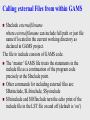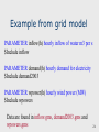
1
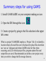
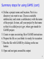
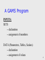
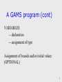
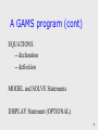
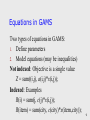
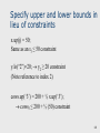
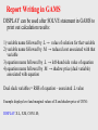
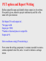
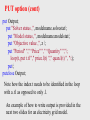
GAMS for Solving Mathematical Programming Problems G. Cornelis van Kooten REPA Group University of Victoria 1 Powerful software for solving LP, QP, NLP, IP, MIP, MINLP and CGE models. Easy to use when setting up large problems: much easier than Excel, Matlab, etc. More powerful than Excel, Matlab, Maple and other packages for solving very large linear and non-linear programs Enables researcher to access a variety of powerful solvers using the same written code. Solvers include Minos, CPLEX, ConOpt, Lindo, XA, and any other commercial and non-commercial solver that is available. Excellent documentation (e.g., McCarl’s User Manual) at www.gams.com Numerous sample programs available in model library at http://www.gams.com/modlib/modlib.htm 2 GAMSIDE: Windows graphical interface to run GAMS GAMS: General Algebraic Modeling System plus IDE: Integrated Development Environment 3 Summary steps for using GAMS 1. Install GAMS &IDE on your computer making an icon 2. Open the IDE through the icon 3. Create a project by going to the file selection in the upper left corner. What is a project? GAMSIDE employs a ‘Project’ file (1) to identify a location where all saved files are to be placed (to place files elsewhere use ‘save as’ dialogue) and where GAMS looks for files when executing; and (2) to which project files, program option files and output files are saved. Recommended you define a new project every time you wish to change the file storage directory. 4 Summary steps for using GAMS (cont) 4. Define a project name and location. Put it in a directory you want to use. Choose a suitable subdirectory and create a subdirectory with the name of the project. In turn, call your project by that name so that it is called project.gpr, where gpr stands for GAMS project. 5. Create or open an existing file of GAMS instructions 6. Prepare the file so you think it is ready for execution 7. Run the file with GAMS by clicking on the run button 8. Open and navigate around the output 5 A GAMS Program INPUTS: SETS -- declaration -- assignment of members DATA (Parameters, Tables, Scalars) -- declaration -- assignment of values 6 A GAMS program (cont) VARIABLES -- declaration -- assignment of type Assignment of bounds and/or initial values (OPTIONAL) 7 A GAMS program (cont) EQUATIONS -- declaration -- definition MODEL and SOLVE Statements DISPLAY Statement (OPTIONAL) 8 Equations in GAMS Two types of equations in GAMS: 1. Define parameters 2. Model equations (may be inequalities) Not indexed: Objective is a single value Z = sum((i,j), a(i,j)*x(i,j)); Indexed: Examples R(i) = sum(j, c(j)*x(i,j)); R(item) = sum(city, c(city)*x(item,city)); 9 Example problem: Minimize transportation costs min cij xij ($) j i s.t. xij a i (supplylimit at plant i ) j x ij b j (satisfy demand at market j ) i See http://www.gams.com/docs/example.htm 10 SETS i plants /Seattle, San-Diego/; j market /NY, Chicago, Kancity/; PARAMETERS a(i) capacity at plant i / Seattle 350 San-Diego 600 / ; b(j) demand at market j / NY 325 Chicago 300 Kancity 275 / ; distance in ‘000s miles; TABLE d(i, j) Seattle NY 2.5 Chicago 1.7 Kancity 1.8 San-Diego 2.5 1.8 1.4 SCALAR f freight cost in $ per ‘000s miles PARAMETER c(i,j) c(i,j) = f * d(i,j)/1000; VARIABLES x(i,j) shipment quantities z total costs in k$; Positive variable x; /8/ ; transport cost in k$ per unit ; EQUATIONS supply(i) supply limit at plant i demand(j) satisfy demand at market j cost objective function is to minimize cost ; cost.. z =E= sum((i,j), c(i,j)*x(i,j)); supply(i).. sum(j, x(i,j)) =L= a(i); demand(j).. sum(i, x(i,j)) =G= b(j); MODEL transport /all/; SOLVE transport using LP minimizing z; DISPLAY x.l, x.m ; Specify upper and lower bounds in lieu of constraints x.up(j) = 50; Same as an xj ≤ 50 constraint y.lo(“2”)=20; y2 ≥ 20 constraint (Note reference to index 2) cows.up(‘3’) = 200 + ½ x.up(‘3’); cows3 ≤ 200 + ½ (50) constraint 14 Report Writing in GAMS DISPLAY can be used after SOLVE statement in GAMS to print out calculation results: 1) variable name followed by .L → value of solution for that variable 2) variable name followed by .M → reduced cost associated with that variable 3) equation name followed by .L → left-hand side value of equation 4) equation name followed by .M → shadow price (dual variable) associated with equation Dual slack variables = RHS of equation – associated .L value Example displays level and marginal values of X and shadow price of CON1: DISPLAY X.L, X.M, CON1.M; PUT option and Report Writing Define output file name and identify where output is to be written. If no path is given, default is project subdirectory and file is file name with .put extension file Output /D:\work\output.txt/ ; *Set page width Output.pw=5000; *Number of decimal places in output file Output.nd=0; Solve modelname using LP maximizing z; Now comes the writing component. A comma is needed to create a comma separated value file, and a / is used to indicate a carriage return. PUT option (cont) put Output; put "Solver status ,", modelname.solvestat/; put "Model status ,", modelname.modelstat/; put "Objective value ,", z /; put "Period" "," “Price" "," “Quantity" ","/; loop(t, put t.tl "," price.l(t) "," quan.l(t) ", "/;); put/; putclose Output; Note how the index t needs to be identified in the loop with a .tl as opposed to only .l. An example of how to write output is provided in the next two slides for an electricity grid model. Calling external Files from within GAMS $Include externalfilename where externalfilename can include full path or just file name if located in the current working directory as declared in GAMS project. The file to include consists of GAMS code. The ‘master’ GAMS file treats the statements in the include file as a continuation of the program code precisely at the $Include point. Other commands for including external files are: $Batinclude, $Libinclude, $Sysinclude $Oninclude and $Offinclude turn the echo print of the include file in the LST file on and off (default is ‘on’) Example from grid model PARAMETER inflow(h) hourly inflow of water m3 per s $Include inflow PARAMETER demand(h) hourly demand for electricity $Include demand2003 PARAMETER wpower(h) hourly wind power (MW) $Include wpowers Data are found in inflow.gms, demand2003.gms and wpowers.gms 21 Comma Separated Value (CSV) Files Spreadsheets and other programs (e.g., Matlab) can read and write CSV files o Commas separate fields o Text items can be in quotes $ondelim – tells GAMS that entries which follow are in CSV format $offdelim – tells GAMS to ‘turn off’ use of CSV format Examples using CSV format SETS K index k /K1*K3/ J index j /J1, J2, J3/; TABLE CSVEX1(K,J) Data in csv Format $ondelim dummy, J1, J2, J3 Note use of ‘dummy’ as K1, 16, 34, 12 the ‘placeholder’ in a table (see also below) K2, 3, 11, 5 K3, 52, 16, 4 $Offdelim 23 Alternatively an external file can contain the table: SETS K index k /K1*K3/ J index j /J1*J3/; TABLE CSVEX2(K,J) data in csv format $ondelim $Include externalcsvdatafile $offdelim 24 The file externalcsvdatafile.gms contains: dummy, J1, J2, J3 K1, 16, 34, 12 K2, 3, 11, 5 K3, 52, 16, 4 Note: ‘dummy’ is needed in the csv format to use up the space over the set elements defining the table rows – in the first row, first column. Consider this example in GAMS and Excel Max Z = 3 x1 + 2 x2 + 0.5 x3 s.t. x1 + x2 + x3 10 x1 – x2 3 x1, x2 ≥ 0 Three equations; x3 is not constrained (‘free’). The GAMS setup and solution are provided on the next slides. 26 GAMS Model $Title McCarl & Spreen Chapter 3 Example SETS i index 1 /1*3/ j index 2 /1, 2/ ; PARAMETER b(j) rhs constraint values / 1 10 2 3 / ; TABLE a(j,i) Table of technical constraints 1 2 ; 1 1 1 2 1 -1 3 1 0 PARAMETER c(i) coefficients in obj /1 3 2 2 3 0.5/ ; VARIABLES z objective value x(i) activities ; EQUATIONS OBJ Objective function CON(j) Constraint ; * ------------------------------------------------------------* Construction of the actual LP model * ------------------------------------------------------------OBJ .. z =E= sum(i, c(i)*x(i)); CON(j).. sum(i, a(j,i)*x(i)) =L= b(j); MODEL McSpreen /all/; x.lo(‘1’)=0; x.lo(‘2’)=0; SOLVE McSpreen using LP maximizing z; Solution to previous GAMS problem Notice that GAMS provides a solution Now consider the solution in Excel Consider both the PRIMAL and the DUAL! PRIMAL Max Z = 3 x1 + 2 x2 + 0.5 x3 s.t. x1 + x2 + x3 10 x1 – x2 3 x1, x2 ≥ 0 DUAL Min R = 10 y1 + 3 y2 s.t. y1 + y2 ≥ 3 y1 – y2 ≥2 y1 y1, y2 ≥ 0 = 0.5 Any attempt to solve either the Primal or the Dual problem within Excel resulted in “The SET CELL values do not converge”. Attempts to solve it as a NLP rather than LP did not help in this regard. Excel does not appear able to solve this simple LP. Actually, since the problem is unbounded it gives infinite values in the cells that are to be changed. Recall: Unbounded PRIMAL means an infeasible DUAL, and vice versa 34 Final Comments Excel does not appear to be a reliable solver Neither can Matlab solve the above problem Matlab and Excel are generally okay for mid-size LPs and small NLPs, but not larger models (but in this case they cannot even ‘solve’ a small LP) GAMS is a preferred platform because of its power to solve even the smallest and extremely large problems (with millions of constraints) 35