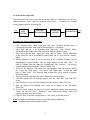
1
PC-SIGNAL
TM
Basic Module
User Manual
AI Signal Research, Inc.
3411 Triana Blvd., SW
Huntsville, AL 35805
(256) 551-0008
http://www.aisignal.com
February 2003
ASRI PROPRIETARY INFORMATION
1.0
TABLE OF CONTENTS
Introduction..........................................................................................................................1
2.0
Input data file selection and Header Information.................................................................6
2.1
Input Data File Selection..........................................................................................6
2.2
View Header File .....................................................................................................6
2.3
Change Header File..................................................................................................8
3.0
Reference Window...............................................................................................................9
3.1
Reduction Sliding Window......................................................................................9
3.2
Reference Window Menu ......................................................................................11
3.3
RPM Tracking in Reference Window....................................................................11
3.4
Processing Example in Reference Window...........................................................13
4.0
Function Window...............................................................................................................14
4.1
4.2
4.3
Signal/Function Menu Group ................................................................................14
Processing Example in Function Window.............................................................16
Function Window Button (Group) .........................................................................26
4.3.1 Option ........................................................................................................27
4.3.2 Quick ........................................................................................................35
4.3.3 Open/Save Setting......................................................................................35
4.3.4 Processing Time Frame..............................................................................36
4.3.5 Time Moving Group ..................................................................................36
4.3.6 M-Menu in Function Window ...................................................................38
5.0
3D Plot Window.................................................................................................................41
5.1
Spectrogram ........................................................................................................43
5.2
Waterfall
........................................................................................................44
5.3
3D Bi-Coh
........................................................................................................46
6.0
Generate data ....................................................................................................................48
6.1
Generate Filter Data ...............................................................................................48
6.2
Generate Decimation Data .....................................................................................50
6.3
Generate Envelop Data ..........................................................................................52
6.4
Generate Order Tracking Data ...............................................................................54
6.5
Generate PSEM Data .............................................................................................56
7.0
Utility ................................................................................................................................58
7.1
Extract/Merge File .................................................................................................58
7.2
Other Data Conversion...........................................................................................60
8.0
Page Setup
....................................................................................................................61
9.0
Batch
....................................................................................................................62
10.0
Technical Section...............................................................................................................64
Introduction to PC-SIGNAL™
1.1 Introduction
PC-SIGNAL™ is a PC-based dynamic signal analysis software package running under the PC
Window Environment. The package makes signal processing a simple task for analyzing
vibration, acoustic, strain, or other dynamic signal measurements. Other than its general capability
for spectral/waveform analysis, it includes a number of specialized signal analysis techniques. The
special techniques are useful for engine/machinery diagnostic evaluation, bearing/gearbox and
drive train signature analysis, and vibration signature analysis. The package saves enormous
amounts of time by eliminating the programming effort that used to be required to perform
sophisticated signal analysis. PC-SIGNAL simplifies every aspect of the signal processing
operation by effective application of its graphical user interface. It expedites all steps from
importing raw signal data files through choice of processing algorithm to outputting the results.
PC-SIGNAL offers:
•
•
•
•
•
•
•
•
•
•
•
•
Latest technology for signal analysis
User-friendly GUI control of program options
Powerful visualization
Audio playback to PC Speaker
Ease of report & presentation generation - provides various output format in a standard
hard copy data plot, or electronics copy in bitmap format.
Automate large/repeated data processing tasks with batch mode
No Programming required
Display large number of data channel plots simultaneously - User can select the number of
processed data plots to be displayed and printed simultaneously with easy selection of the
colors and labels for each plots from a menu
More than 50 analysis techniques available - User can change analysis option on the fly
through the user interface and see results instantly.
Easy selection of the processing time blocks from a Reference Window display
Move the processing time block through the duration of the entire measurement
Cost effective system: PC-Based
The user gets immediate visual feed back with graphical data plots in either two-dimensional or
three-dimensional graphs.
PC-SIGNAL lets a user quickly locate signal components. The program provides tools to enhance
the presence of components to demonstrate their presence in the data plots more prominently.
Several mathematical routines and filtering processes to reduce unwanted noise and other signal
contamination are built in. The package provides an array of spectral analysis procedures that help
a user to make intelligent conclusions for many applications. PC-SIGNAL procedures include:
•
•
Waveform Statistical Metrics
Auto- and cross- Spectral Analysis with Multiple window selection to minimize data
leakage
1
•
•
•
•
Linear Correlation/Coherence analysis
Transfer Function & Phase tracking
3D Time/Frequency Waterfall & Spectrogram
Filtering (High-Pass, Low-Pass, Band-Pass ) with easy selection of filter type and
parameters graphically
• Spectral Components Tracking
• Histogram & Statistics (Mean, RMS, Skewness, Kurtosis, Max/Min, Crest Factor, etc)
• Shock Spectrum
• Unique Function Window design for displaying multiple process results for a given
measurement simultaneously or multiple measurement with a selected processing method.
PC-SIGNAL provides the user with a batch processing capability where many measurements can
be processed with a common sequence of algorithm processing parameters and display format.
Under batch, the program processes each selected measurement and prints the result unattended.
PC-SIGNAL offers multiple user-friendly methods to manipulate data. The user can inspect the
data stream simultaneously in the time domain (in any or all moment format), the spectral domain,
and the cross correlation format, in either or both time and spectral based display configurations.
Display smoothing options allow the choice of a large number of parameters while maintaining
the integrity of the original data stream.
PC-SIGNAL provides easy visual interpretation of a user’s signal analysis results. The program
automatically plots peaks, contours, and surfaces to enhance the significance of results. The users
can clearly present results with control over titles, fonts, colors, scaling, labels, grid and plot types.
The results can be saved as bitmap files for future easy recall.
The Advanced Module includes a number of specialized diagnostic signature analysis techniques
for rotary machinery diagnostics and bearing/gearbox diagnostics. These analysis tools are also
useful for signal enhancement, fault detection and anomaly identification for diagnostic
evaluation.
•
•
•
•
•
•
•
•
PSEM - a phase synchronized technique for RPM-related Signal Transformation and
Identification
CPLE™ - a signal enhancement technique for RPM-related vibration signal.
RPM Coherence - a spectral type of coherence function representing the phase correlation
of any vibration components w.r.t. RPM.
Nonlinear Bi-&Tri-spectral/coherence analysis - nonlinear correlation detection and
Identification
Envelop Analysis - high frequency envelop analysis for amplitude demodulation
CPWBD - coherent phase demodulation technique for pump cavitation detection
Order Tracking - order analysis
STA/SPA - synchronized time/phase average for gearbox vibration signal analysis
2
A customized version of PC-SIGNAL can be built for any special requirement from the PCSIGNAL module such as:
•
Automating/integrating special analysis procedures
•
Monitoring - database & trend analysis
PC-SIGNAL has been applied to:
•
•
•
•
•
•
Space Shuttle Main Engine (SSME) post test/flight diagnosis & anomaly identification
Weapon system vibration measurement data analysis & specification development
Helicopter drive-train (gearbox & bearing) diagnostics
Dynamic characterization of turbopump wind tunnel, water flow test
Radar antenna servo drive-train health monitoring & diagnosis
FedEx conveyor belt bearing fault detection.
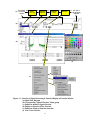
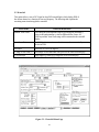
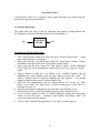
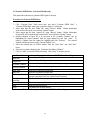
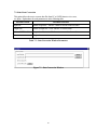
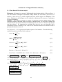
1.2 Program Overview
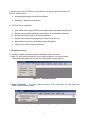
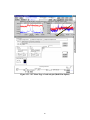
PC-SIGNAL program execution is performed through the main menu items:
(1) File - To select and open a data file for processing and analysis, view/edit the header
information of the opened data file, and select default printer to print output to.
Figure 1.1 – File Menu Options
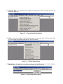
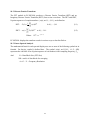
(2) Signal Processing – To perform signal processing of the opened data file and display the
results in various function format.
Figure 1.2 – Signal Processing Menu Options
3
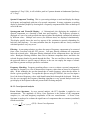
(3) Generate Data - To perform various signal processing of the selected data file and store the
result in an output file.
Figure 1.3 – Generate Data Menu Options
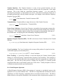
(4) Utility – Provide a number of utility tools to extract or merge data from ASCII or binary files,
or to convert data file in other format into PC-SIGNAL format.
Figure 1.4 – Utilities Menu Options
(5) Page Setup - To configure the overall page setup (x/y scale, labels, color etc.) for all plots displayed
either on screen or in print out. Also used to set line colors for the selected plot.
Figure 1.5 – Page Setup Menu Options
4
(6) Batch – To automate a sequence of processing tasks as a batch job.
(7) Window – To Rearrange multiple windows displayed on screen.
(8) Help – To provide on-line help
1.3 Mouse Button Operation in PC-SIGNAL
1.3.1 Left Mouse Button
In PC Signal, mouse has several uses. Whenever mouse moves over a graph, a marker appears.
The crossing point of the marker can be used to determine exact coordinates of points on the
graph. The coordinates are displayed on top portion of the page. If there exists more than one
graph, the coordinates corresponds only to the current graph the mouse pointer is active, denoted
by red color “M” on upper right hand corner.
1.3.2 Left Mouse Single Click
While the mouse pointer is on a graph, user can click once to find a peak nearest to the current
mouse position. The peak found is governed by the “Peak Frequency Locking Mouse Marker
Window,” set in the “Processing Parameters.”
1.3.3 Left Mouse Double Click
If left mouse button is double clicked when it is within a graph box, a zoom window containing
that graph will appear. In the “Zoom Window,” user can perform any kind of graph manipulation
as if it were still in the “Function Window.”
1.3.4 Left Mouse Pressed-Drag-and-Release
This implies to the case when left mouse button is pressed down, dragged and released. This
action results in zooming the graph the mouse pointer is currently on. If “Sync Zoom” is on, all
graphs in the “Plot Window” will be zoomed in. To return to normal view, select “Zoom Out” in
“Right Mouse Click.”
1.3.5 Right Mouse Button
The right mouse button, when used in the “Function Window,” invokes a set of options such as
printing the plots, save the plot in either ASCII or bitmap file format, perform frequency
matching, etc.
5
2.0
File (Input File Selection, View Header Information, and Printer
Selection)
“File” Menu item allows a user to select a data file for processing, view/edit the
header information of the selected data file, and select the default printer to print
outputs.
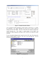
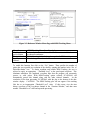
2.1 “Open DataFile” - Input Data File Selection
Figure 2.1 – Input Data File Selection
The first action by a user is to select the Data File to be processed. Click “File” -> “Open
Datafile” to select the desired data file for processing.
Clicking on the drop-down button will display the previous selected data files. The file
names are sorted in the most-recently used order. Select on one of these file names will
result in opening that data file for processing.
Each data file is represented by 2 different parts (2 different files in disk):
(1) XXXX.dat
- Contains data points in binary format.
(2) XXXX.menu - Contains header information (e.g. Sampling Frequency, Time, number
of channel, Channel Information, etc.)
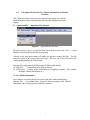
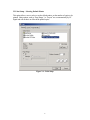
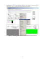
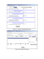
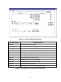
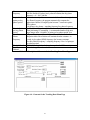
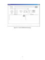
2.2 View Header Information
Once a data file is selected, the user can view the data file’s header information by
selecting “File” -> “View Header Info.” Figure 2.2 shows an example of the “Channel
Information” sub-window that pops up after the selection.
6
Figure 2.2. Channel Information Window
User can change the header information by directly typing in each entry box. To change
the information in the channel information box, first select the desired channel by
clicking on the line that channel. The user can then make any changes by typing in the
channel information box. Click “Update” to confirm changes for each channel. After
entering new channel information and clicking “Add” will add a new channel into current
header file.
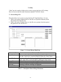
To save the updated information back into the file, click “OK,” and a file selection subwindow as shown in figure 2.3 will pop. Click “Save” to save the header file. User can
also specify a different header file name.
Figure 2.3 - Save Header File
7
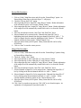
2.3 Print Setup – Selecting Default Printer
This option allows a user to select or set the default printer, set the number of copies to be
printed. Other options, such as “Page Range,” or “Layout” are set automatically by PC
Signal and will not have an effect on the printed copies.
Figure 2.4 – Print Setup
8
3.0 Signal Processing – Reference Window
“Signal Processing” allows a user to perform various signal processing of the selected
data file and display the results in a number of function format. Signal processing can be
performed in the following 3 different Windows:
(1) Reference Window - This option provides a time reference of the overall data file by
displaying its reduced (or compressed) waveform or statistics so that the user can
conveniently locate and select any desired time segment for detailed analysis in the
“Function Window.”
(2) Function Window - This processing window enables a user to process data using any
of the available processing functions and display the processing result in 2D X-Y
format within multiple sub-windows. Most of the signal processing of PC-SIGNAL
is performed in this option.
(3) 3D Plot Window - This window allows the user to display 3D Spectrogram,
Waterfall, Topo, or 3D Bi-Coherence graphs.
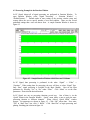
3.1 Reduction Sliding Window in Reference Window
This Reference Window provides a time reference of the data file by displaying an
overall picture of the entire test profile/characteristic in the form of reduced statistics so
that the user can conveniently locate and select any desired time segment for detailed
analysis in the “Function Window.” In this “Reference Window,” raw data waveform is
reduced into a readily comprehensible plot as a function of time in the form of reduced
statistics (Mean, RMS, Skewness, Kurtosis), or compressed waveform (Max/Min) or
RPM (if a key-phasor measurement is available) for the selected channels. Such
waveform reduction is performed through a sliding “Reduction Sliding Window” as
depicted in figure 3-1. Within each sliding Reduction Sliding Window, a single reduction
value (two for Max/Min reduction) will be generated and plotted. As a result, an overall
reduced waveform or statistics will be displayed in the “Reference Window” plot. This
option provides a convenient mean to select time for further processing in the “Function
Window” by dragging mouse over the reduced waveform.
9
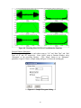
(a) Snapshot Time History of Original Waveform
Reduction
Window
(b) Reduction Waveform (RMS) over
the Entire Time Period of Datafile
Figure 3.1 - (a) Reduction Sliding Window; (b) RMS Reduction Waveform
Figure 3.2 - Menu Page for Reference Window
10
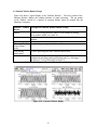
3.2 Reference Window Menu
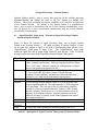
Figure 3.2 shows the menu page for the “Reference Window.” It allows a user to choose
the reduction type (Mean, RMS, Skewness, Kurtosis, etc.), reduction start/end time,
reduction size and measurement(s) to be processed. Explanations for each menu item are
as follows:
Table3-1 : Menu Items of Reference Window’s Menu Page
Menu Item Name
Menu Item Description
Reduction type
Defines reduction type to be applied to the raw data. Six choices
available are available: Mean, RMS, Max/Min, Skewness, Kurtosis, and
Crest Factor. Can choose RPM profile option if the key-phasor
measurement is available.
Reduction Start
Time
This is the start time for data reduction within the Reference Window
(default is the start time of data file).
Reduction End
Time
This is the end time for data reduction within the Reference Window
(default is the end time of data file)..
Reduction Size
Reduction sliding window, in terms of number of data points, in setting
plot density.
Channel Available
Name of each measurement channel available in the data file
Channel Selected
This display box shows the measurement channel(s) that have been
selected for processing.
The user can select a channel for reduction by highlighting the channel name in the
“Channel Available” list and clicking “Add.” Highlighting and then clicking “Remove”
will deselect the channels. The “Start” button, when clicked, will commence the data
reduction. As a result, a “Reference Window” plot will appear that contains graphs of
reduced data of selected the selected channels. The “RPM Tracking” window of the
speed channel will also appear if selected. Clicking “Stop” will stop the processing.
3.3 RPM Tracking in Reference Window
This RPM Tracking option in the Reference Window provides the user a way to display
an overview RPM profile of the speed (key-phasor) channel in a data file. Figure 3-3
shows the “Reference Window” menu page when the “RPM Tracking” option is selected.
11
Figure 3-3: Reference Window Menu Page with RPM Tracking Menu
Menu Item
No. Of pulses
per Revolution
Threshold Level
Key Phasor
Channel
RPM Tracking Menu Item Description
Number of pulses per revolution of the shaft that was recorded in the
key-phasor measurement
Threshold level applied to the key-phasor pulses for RPM counting.
Select the key-phasor channel
To enable this function, first click on the “Yes” button. Then specifies the number of
pulses that was recorded per revolution of the shaft by entering this number in the “No. of
Pulses/Revolution” box. To obtain expedient and reliable RPM Tracking, the user is
advised to apply an appropriate “Threshold Level” to the speed signal waveform. This
eliminates anomalous low amplitude waveform blips that the program will erroneously
process as valid pulses. With RPM-Tracking option selected, PC-SIGNAL will
automatically process this channel along with the other selected channels. At the
conclusion of the data processing, PC-SIGNAL adds the plot to the bottom of the data
window display. CAUTION: The RPM-Tracking plot will not appear if the tracking
fails due to an inappropriate “Threshold Level” value. If this occurs, view the time
history waveform of the key-phasor channel in the “Function Window,” and then enter
another “Threshold Level” value and repeat the processing.
12
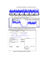
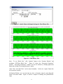
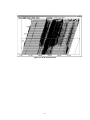
3.4 Processing Example In Reference Window
Setup the RPM Tracking parameters as shown in Figure 3.3. Data file used is
“ISO_Test1.dat.” Click “Start” to begin processing. Figure 3.4 shows the resulting
Max/Min Reduction along with the RPM profile.
Figure 3.4 - Example of Reference Window Display
13
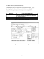
4.0 Signal Processing – Function Window
Function Window enables a user to process data using any of the available processing
algorithms/functions and displays the result in 2D X-Y Format over multiple subwindows. Most of the processing and analysis capabilities of PC-SIGNAL are performed
in this Function Window. The software is very flexible because it is programmed to
allow a user to process a measurement with one or more functions simultaneously, or the
user can process two or more measurements simultaneously using one or more functions
for each selected measurement.
4.1
“Signal/ Function” Menu group - Selection of Signal Processing & Display
Format in Function Window
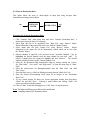
Figure 4.1 shows the selection of signal processing along with its display function
formats in the “Function Window.” All signal processing in Function Window is based
on the signal flow diagram in figure 4-1(a) with its corresponding menu selection in the
“Signal/Function” Menu group in figure 4-1(b). This “Signal/Function” menu group
defines the signal flow and its output display format for each sub-plot. Table 4-1 lists the
description of the menu items in the “Signal/Filter/Function/Channel” Menu group
Menu Item
Signal
Filter
Factor
Function
Channel
Line
Thickness
Color
Description of “Signal/ Function” Menu group
To select the type of signal processing on of the input raw signal x(t),
(“Raw” indicates no processing). Select by using drop-down box (Figure
4-1c). Click “menu”, whenever it appears, to set the parameters of signal
menu; menu number used appears to the left.
To select the filtering and its parameters on the post-processed signal y(t),
if ‘Yes’ is chosen. By click “menu” (Figure 4-1d), the filter type
(bandpass, lowpass, highpass) and parameters (filter order and cutoff
frequencies, etc.) along with its menu number can be selected.
To apply a scaling factor(multiplier) to the post-filtered signal z(t).
To select the type of signal function (Figure 4-1e), to be generated from
the post-amplified signal w(t). The output function fx(.) will be displayed
in x/y plot format. The x-axis can be time (e.g. time history, reduction,
tracking etc.), time lag (correlation function), frequency (PSD, Transfer
function, coherence, shock spectra, etc.), or other parameter such as bifrequency for bi-coherence function.. Function parameters can be set,
whenever necessary, by clicking “menu” button, appeared to the right of
menu number being used.
To specify the input channel x(t) to be processed.
To specify the thickness of plotting line for function display
To specify the color of plotting line for function display(Figure 4-1f)
Table 4.1 - Description of “Signal/ Function” Menu group in Function Window
14
Raw Signal x(t)
(a) of selected
channel
y(t) BandPass
Signal
Processing
Filtering
z(t) Amplitude
Scaling
w(t)
Function
fx(.) X/Y Plot of
the Resulting
Function
(b)
(c)
(d)
(f)
(e)
Figure 4.1 - Selection of Signal Processing & Function Display in Function Window
(a) Signal Flow Diagram
(b) Corresponding “Signal/ Function” Menu group
(c) Pull-down menu for Signal Selection
(d) Pull-down Menu for Filter Selection
(e) Pull-down Menu for Function Selection
(f) Line Color Selection
15
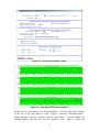
4.2 Processing Example in the Function Window
In PC Signal, almost all of signal processing are performed in Function Window. To
open Function Window, select “Signal Processing” -> “Function Window” ->
“Default/Custom/…” Default results in same setting as the previous window setup, and
custom allows the user to specify number of rows and columns. There are also several
predefined settings that a user can choose from. A sample Function Window is shown in
figure 4.2.
Figure 4.2 - Sample Function Window with 4 Rows and 1 Column
In PC Signal, data processing is performed in the order: “Signal” -> “Filter” ->
“Function.” When setting data for processing, the user will have to select “Signal” first.
Only “Raw” signal processing is available in the Basic Module. Next set the Filter
parameters by selecting “Yes” or “No” under “Filter.” Click “Menu” to set the filter
parameters. Next select the desired function.
In PC Signal, one can set processing functions several way. One of them is via the
“Quick” button in the Function Window. “Quick” menu allows a user to apply the same
processing function to different channels.
When clicked, “Quick Menu” window
appears. Set parameters as shown in figure 4.3. Click “OK” when done. Next enter
“100” in “Start Time” box, click “1 Block.” Click “Start Plot” to begin processing and
plotting. Resulting plot is shown in figure 4.4.
16
Figure 4.3 - Quick Menu with Sample Settings for Time History Plot
Figure 4.4 - Time History Plot
Note: To set “Block Size,” click “Options” button in the “Function Window” and
set/change “FFT/Data Block Size.” Figure 4.5 shows the “Processing Parameters”
window. “Processing Parameters” window can also be invoked by clicking right-mouse
button and selecting “Processing Parameters” option.
“Start Time” and “End Time” can be entered manually. In this case “Apply” button has
to be pressed to confirm.
In Function Window, you can zoom into any time or frequency range by press-drag-andrelease left mouse button. Figure 4.6 shows a sample in zooming in to particular time
range.
17
Figure 4.5 - Processing Parameters Menu
Figure 4.6 - Time History Plot when Zoomed In
Another way to set processing is via “Processing Menu.” It can be called up by clicking
on the “M” on top right corner of a plot. Figure 4.7 shows the “Processing Menu.”
Setting functions to process is similar to that of “Quick Menu.” For this example, the
Function Window with four rows and two columns is used. Figure 4.8 shows the
18
resulting plot of “Wave Form Reduction” functions. One will have to click on “M” for
each function. This way, multiple functions can be plot on same window.
Figure 4.7 - Processing Menu with Wave Form Reduction Function Selection
19
Figure 4.8 - Resulting Plot of Six Wave Form Reduction Functions
Function Window (Histogram)
For this purpose, change the row and column setup to “2x1” and “Start Time” and “End
Time” to “0” and “50” respectively. From “Quick” menu in Function Window, select
“Histogram” as the processing function. Click “Menu” button to set “Histogram”
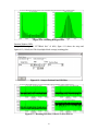
parameters. Figure 4.9 shows a sample setting and figure 4.10 shows the resulting plot.
Figure 4.9 - Sample Histogram Setting
20
Figure 4.10 - Resulting Histogram Plot
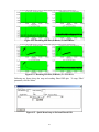
Function Window (PSD)
Using “2x2” setup, and “FFT/Block Size” of 4096, figure 4.11 shows the setup and
figures 4.12 (1 block) and 13&14 (multiple blocks average) resulting plots.
Figure 4.11 - Setup to Perform Four PSD Plots
Figure 4.12 - Resulting PSD Plot (1 Block) T=50 to 50.4 sec
21
Figure 4.13 - Resulting PSD Plot (50 Blocks) T=50 to 100 sec
Figure 4.14 - Resulting PSD Plot (50 Blocks) T=-50 to 0 sec
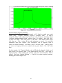
Following two figures shows the setup and resulting filtered PSD plot. To setup “Filter”
parameters, click on “Menu.”
Figure 4.15 - Quick Menu Setup to Perform Filtered PSD
22
Figure 4.16 - Resulting Filtered PSD Plot
Function Window (Frequency Matching)
“Frequency Matching” function is implemented in PC Signal to enable users easily
identify peaks. “Frequency Matching” requires a “Frequency Table.” To setup a
“Frequency Table,” click right-mouse button and select “Frequency Matching Setup.”
“Frequency Matching/Marking Setup” window, figure 4.17 appears. Next click “New”
to setup a new table. Enter “ISO_Test1A” as the name. Next another window, figure
4.18, pops up. This is where all the peak information is entered. To enter peak
information, enter peak “Symbol,” peak “Description,” and its frequency, fixed or
relative to reference frequency. Next check “Active” and click “Add.” When a peak is
not active, its frequency will not be matched with any peak found. Click “OK” when
done.
For this example, “1x1” Function Window with a PSD plot for channel 1, block size of
4096, from 0 to 210 second is used. To use whole data file, click “Full.” Click “Start” to
begin processing. When resulting plot is shown, make sure correct Frequency Table is
selected. Then select “Multiple Matching” -> “One Plot” to perform frequency matching.
Resulting plot is shown in figure 4.19.
23
Figure 4.17 - Frequency Matching/Marking Setup
Figure 4.18 - Frequency Table Setup
24
Figure 4.19 - Resulting Frequency Matching Plot
25
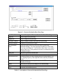
4.3 Function Window Button (Group)
Figure 4.20 shows a typical display of the “Function Window.” The lower portion of the
Function Window displays the resulting functions of signal processing. The top portion
of the Window consists of a number of operation buttons which are grouped into the
following 6 categories:
Function Window Description of Function Window Button (Group)
Button
Option
To select processing parameter, number of row/column for plotting,
zoom, marker, basket, save, print, etc.
Quick
A quick way to select the same processing/function format for all
channels.
Open/save Setting
To save/recall Function Window plot setting.
Processing Time
To select the processing time frame.
Frame buttons
group –
Time Moving
To move processing time frame within the data file time.
button group
M-Menu
Menu of each sub-plot - To select signal processing & display for each
individual sub-plot along with its plot format (color, x/y –axis range,
linear/log, etc.) (to be discussed in section 4.3)
Table 4.2 - Description of Function Window Button (Group)
Figure 4.20 - Function Window Display
26
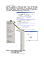
4.3.1 “Option” Button
This button is the same as a right-mouse click on any part of the Function Window.
When the Option button (or the right mouse button) is clicked from the “Function
Window,” it opens a pop up option menu (figure 4.21). The Option button allows user to
select processing parameter, number of row/column for plotting, zoom, marker, basket,
save, print, etc. The description of each menu item is shown in Table 4.3.
(b)
(d)
(a)
(c)
Figure 4.21 (a) Option (Right Mouse) Button Menu
(b) Processing Parameter Menu
(c) Row/Column Setup
(d) Custom row/column for page layout
27
Menu Item
Processing
Parameters
Row/Column
Setup
Description of Menu Item in Option Button
The “Processing Parameter” menu allow user to select (1) FFT/Data Block
size for spectral analysis, (2) Reduction Time for Waveform Reduction (3)
Window application for spectral analysis. (4) Overlap for block processing (5)
Peak frequency lock-in for mouse marker
Specify the number of row and columns the current function window will
have. See Figure 4-3c.
Frequency
Matching
Setup
Sets up the frequency table for frequency matching. Additional matching
parameters are also set here.
Single
Matching Off
When chosen, frequency matching for single peak is turned on. After this
option is turned on, when left mouse button is clicked on a plot, the peak
within “Mouse Marker Bandwidth” is located and its frequency is matched
using existing parameters.
When chosen, frequency matching for all peaks is turned on. After this option
is turned on, when left mouse button is clicked on a plot, the all peaks are
located and peak frequencies are matched using existing parameters.
When chosen, a new “Function Window” plot, containing the statistics of the
current plot, pops up. The plot is in the form of a Histogram. Current or all
plot statistics can be drawn depending on the selection. Figure 4.22 shows the
resulting statistics plot of figure 4.20.
Display the list of peak that matches the criteria specified by the user. Figure
4.23 shows the resulting peak listing using 5 (SNR) and 10 (Freq Window).
Marks the harmonics of the specified frequency that is within the range.
Figure 4.24 displays the markings of 500 Hz.
After “Zoom In”, use this option to return to the original plot of overall xrange. Zoom in is accomplished by click, drag and release left mouse button.
When chosen, synchronized zoom option will be turned on. This enables the
user to zoom in to same range of frequency, or time, of all plots in the
Function Window. It is equivalent to changing the maximum and minimum xaxis values of all plots to some value.
Prints all plots in “Function” window.
Multiple
Matching
Show Statistics
Peak
Harmonic
Marker
Zoom Out
Sync. Zoom
Print
Print with Peak
Label
Print with
Frequency
Synchronized
Marker
Replot
Clear
Show Basket
Content
Prints all plots with peak frequency values.
Prints all plots with peak frequency values matched to existing parameters.
Like “Multiple Matching” then “Print”.
When chosen, synchronized marker option will be turned on. This enables the
user to compare plots from different graph boxes using same marker position.
This option will redraw the plots with updated configurations.
Clear the Function window.
Allows user to see what plot data are stored to be saved into file or further
processing, Figure xx. See section yy for detail information on “Basket.”
Add to Basket
(Single Plot)
To add and store a single plot data within the “Function Window” into a basket
file (to be recalled later for further processing).
Add to Basket
To add and store all plots data within the “Function Window” into a basket file
(to be recalled later for further processing).
28
(All Plot)
Automatic Add
to Basket
(to be recalled later for further processing).
When switched on, this option enables the user of PC Signal to add processed
data, in the “Function Window,” be added into the “Basket” automatically.
Save Bitmap
When switched on, this option adds processed data of the “Function Window”
into the “Basket” without checking the existence of the same result in the
“Basket.”
When chosen, sound option is turned on, and the signal of selected plot will be
played through PC’s speaker allowing user to listen to the signal. See section
4.3.1.2 for more details.
Save the resulting plot into a bitmap file.
Save ASCII
Save a particular plot data into file in ASCII format.
Coordinate
Transformation
Allows the user to transform coordinate from “Time” to “RPM,” “Tau,” etc.
and back.
Peak Tracking
Used in conjunction with the “Play” button. When switched on, this option
tracks the peak amplitude of the desired frequency and display the result in a
separate window.
Check Data
Existence
Sound Off
Table 4.3 - Option (Right Mouse) Button Menu Item Description
Figure 4.22 – Resulting Statistics Plot of Figure 4.20
29
Figure 4.23 – Sample Peak List Plot
Figure 4.24 – Harmonic Marking of 500 Hz
30
4.3.1.1
“Processing Parameter” in “Option” Button
The “Processing Parameter” menu (See Figure 4.21b) allows the user to select/set the
following parameters:
Parameter Name
Parameter Function
FFT/Data Block Size
FFT/Data Block size for processing
Play Execution
Delay
This sets time delay between each block calculation, in msec, minimum is
1 and maximum is 32768.
Block Overlap(%)
This sets the percentage of overlap from one processing block to the next.
Analysis Window
Overlap
This sets the percentage of overlap from one analysis window to the next.
If analysis window is (0-5) sec and overlap is 50%, then next analysis
window is (2.5-5) sec.
Fixed Sliding
Window/Fixed Total
Reduction
This option applies to the “Time Domain Waveform Reduction”
processing only. “Fixed Sliding Window” reduces the time data into 1
point for the reduction set. “Fixed Total Reduction” reduces the time data
to the fixed total number of points regardless of the size of input.
Window Type
Type of window: None, Flat Top, Hamming, Hanning, Kaiser Bessel, and
Rectangular. – Applied to all spectral analysis
No of Application
For Multiple window application. – Applied to all spectral analysis
Peak Frequency
Locking Mouse
Marker Window
The range where the highest peak is to be searched from current mouse
position. This is only used in finding peak. – Applied to frequency
domain function display.
Spectral Type
This option sets the spectral types as “Power Spectrum Density,” “Power
Auto Spectrum,” and “Auto Spectrum.”
Row/Col
Arrangement
This option applies to setting plots using “Quick” menu only. This option
sets the row/column major plot channel assignment.
Histogram Plot Para.
This option is for use in “Statistics” display.
Table 4.4 - Processing Parameters in “Option” Button
4.3.1.2
“Sound” Option in “Option” Button
The user can enable this option, Spectrogram Waterfall Topo, and listen to the sound of
raw data being processed. It can be selected in the Right Mouse Button option. When
that option is switched on, figure 4.25, a sound menu appears. Once this menu is set, the
user can listen to sound of data as the file is being processed. Parameters and their
explanations for this menu are listed in the following table. When using the sound option
in the “Function Window,” turn the sound option on. When clicking on the sub-plot
whose signal to be played, the menu symbol “M” of that sub-plot will turn into “S” to
indicate the sound channel selection. To switch the sound to other channel, simply click
on the next desired sub-plot.
31
Sound menu items
Description of Sound menu items
Gain
D/A Gate
Gain of sound.
Digital to audio gate. All parameters are in engineering unit.
xmax
xmin
Sound On/Off
Maximum x scale.
Minimum x scale.
Switches sound on or off
Sound Speed
Auto Fast/Slow
Determines how fast sound will be played.
PC Signal sets the speed.
Auto Fast/Real Time
Manual
OK
PC Signal will play sound as fast as CPU can handle.
User sets the speed, in percentage.
Confirms the settings.
Cancel
Apply
Discard the settings.
Update to current settings.
Open Menu
Save Menu
Open previously saved sound settings.
Save current settings.
Table 4.5 - Description of Sound menu items
Figure 4.25 - Sound Setting Menu
32
4.3.1.3
“Basket” in “Option” Button
The “Basket” option allows user to save processed data arrays in a basket file, which can
be recalled later for further processing. Typical operation procedure is described below:
1. To save all the plots currently being displayed in the “Function Window” into the
“Basket,” click “Option” (or right mouse button) and select “Add to basket (multiple
plots)”. All data plots shown in the “Function Window” will then be added and
stored into a basket file (unnamed yet). A name for each plot (line) will be assigned
based on its test_ID/Channel_ID/Signal/Function/Info for easy recognition during
recall. This step of adding to basket can be repeated many times to add more plots
into the basket during analysis.
2. To view all plots been saved in the basket, clicking on “Option” (or right mouse
button) and select “View basket.” A “Basket” menu page as shown in Figure 4.26
will be displayed. Clicking “Remove” will remove highlighted data from basket.
Using “Save” to save the current basket to a basket file name.
3. To recall plot files stored in a basket file at a later time, clicking on “Option” (or right
mouse button) and select “View Basket ”and then use “Open” to open the desired
basket file.
4. To plot the recalled plots in the basket file, first click on the desired sub-plot box,
(user might need to clear this sub-plot box). Then choose the desired plot name in the
basket file list by highlighting it, and then click “Add to Plot” button. The recalled
plot will now be displayed in the selected sub-plot box. More than one plot can be
placed in the one sub-lot box.
Each data in the basket can further be manipulated by using “Add” button. A
combination of data in the basket can be obtained by highlighting data, setting “Factor”
and clicking “Add.” This is similar to “Multiple Lines Multiple Functions” in M-Menu
of “Function Window.” Click “Remove” to remove a particular line from the plot in
“Block Manipulation.” “Reset” removes all data. “Add to Plot” draws graph of
manipulated block.
Description of Basket Menu Items
Parameter
Name
Reset
Removes all data from the Basket.
Save
Stores data the basket into a selected basket file.
Open
Allows user to retrieve previous baskets.
Add to Plot
Add All
This option will plot selected data in the last mouse-clicked graph box.
ASCII File
This option will plot selected data in the “Function Window” one line in each
sub-plot box.
Saves the data in the “Basket” into an ASCII file.
33
Excel File
Saves the data in the “Basket” into an Microsoft Excel file.
Table 4.6 - Description of Basket Menu Items
Figure 4.26 - Basket Window
34
4.3.2
Quick
This option allows users to setup page settings quickly by setting the same processing
function for multiple channels. When “Quick” button is clicked, the following window
(figure 4.27) appears.
Figure 4.27 - “Quick” Menu
Explanation of each Quick menu item is as follows:
Menu Item
Start Channel
End Channel
Signal
Filter
Function
OK
Description of Menu Item in Quick Button
Starting channel number for use in Function Window setting.
Ending channel number for use in Function Window setting..
Type of signal to be used in processing data. (same as table 4.1-1)
Filter parameters to be used in data processing. (same as table 4.1-1)
Type of function to be used in data processing. . (same as table 4.1-1)
Confirms the current settings. To cancel, click “x” at top right hand
corner of window.
Table 4.7 - Quick Button Menu Item Description
The channel arrangement is governed by the “Row/Column Arrangement” selection in
the “Processing Parameters.”
4.3.3
Open/save setting
After user set up the various plot formats within a Function Window (such as a 3row by 3
column plot with 1st column showing time histories, 2nd column showing PSDs; 3rd
column showing Histograms), the setting can be save to a “Function Window Setting
35
Menu” which is recorded as a menu number. Such saved page setting can then be
recalled for future usage without having to repeat the setup process again.
4.3.4
Processing Time Frame (PTF) buttons Group
The Processing Time Frame Buttons Group allows the user to select the processing time
frame as described in table 4.8.
Note: Since the Function Window will perform either block-by-block processing or
multiple-block averaging, the user-selected Processing Time Frame will be automatically
truncated to the smaller block time near the PTF. (Block size is set in the “Processing
Parameters” window, discussed in section 4.3.1)
Item
Apply
Grab
1-Block
Full
Description of Menu Item in Quick Button
To manually select a time frame: Enter the desired times in the start/end time
box and then click the “Apply” button.
To Grab the selected time in the Reference Window: (Needs to use in
conjunction with Reference Window). First select the desired time period in
the Reference Window by dragging the mouse pointer directly over the
reduction waveform, and then click the “Grab” button in the Function Window
To choose a time frame with 1 block length: First select the desired start time
either using “Apply” or “Grab”, then click the “1-Block” button. . It value of
block size is set by “FFT/Block Size” in the Option Button (see section 4.2.1)
Start time will remain the same. End time is obtained by adding the quotient
(of block size divided by sampling frequency) to the start time.
To choose the time frame of the entire test data by click the “Full” button.
Table 4.8 - Time Frame buttons Group Menu Item Description
4.3.5
Time Moving Button Group
The time moving button group allows user to move processing time frame within the data
file time as described in table 4.2-8.
Start Plot
Starts data processing and display the result without continuously advancing
to the next time frame. (i.e. plot and freeze with not animation or update)
Play
Start data processing and display the result one time frame at a time and
continuously updates by advancing to the next time frame.
The next time
frame will have the same duration but with its Start Time equals to the end
36
time of current time frame. Animation display is shown with old graphs
being overwritten when new data is processed and ready to be graphed.
Stop
Stop data processing and advancing.
Forward
Advance one time frame and process/display without further advancing
Backward
Move back one time frame and process/display without further action.
Rewind
Goes processing time frame back to the start of data file.
Table 4.9 - Time Moving Button Group Menu Item Description
The horizontal bar appeared in the middle of window indicates where the current block
located, with respect to the whole data file. When Reference Window is activated, the
current processing time frame will also show as a moving bar on Reference Window’s
reduction waveform. The feature allows the user to correlate the timing of information
displayed in Function Widow to the overall test profile.
37
4.3.6
M- Menu in Function Window
As discussed in section 4.3.2, the Quick option allows users to setup page settings
quickly by specifying the same processing function for multiple channels. If user needs
to set up different processing function for multiple channels, it can be achieved using the
M-Menu of each sub-plot. By clicking “M” at the top right corner of each sub-plot box,
an “M” menu page appears, Figure 4.28. Settings for individual sub-plot are done here.
The descriptions of each menu item in the “M” menu Page are listed in table 4.9.
4.3.6.1 Single-Line Option
When Single-Line Option is selected in the M-menu page, there will only be one function
displayed (represented by one plot line) within each sub-plot. The function displayed is
defined by the selection in the signal/filter/function/channel menu group.
Figure 4.28 - “M” Menu Page of each sub-plot (Single Line Option)
38
4.3.6.2 Multi-Line Option
The Function Window is capable of drawing multiple lines within sub-plot(s). In
“Multiple Line-Single Function” mode, (figure 4.29) more than one type of signal will be
drawn in a single sub-plot box. Settings are the same as in “Single Line Single Function”
mode. The user will have to determine how many lines are to be drawn in a particular
sub-plot box and what they will be by entering “No of Lines.” Choosing “Line 1”, “Line
2” etc. allows the user to set each line’s plot format through the same
signal/filter/function/channel menu group. To confirm each line of the graph, the user
needs to press “Update.” If it’s not pressed, the settings for that particular graph will not
be updated.
Menu Item
Menu Item Description of “M” Menu of each sub-plot
Main Title
Sets main title of graph.
X-Axis Title
Sets X-title of graph.
Y-Axis Title
Sets Y-title of graph.
Auto
Sets auto scaling for X and Y-axes.
Manual
Sets scaling for X and Y axes manually.
Type
Sets linear or Log10 scale graph.
Grid
Draws grid of graph in background if chosen.
Colors
Sets background, text, and marker colors.
Signal
Type of signal to be used in processing data. (same as table 4.1-1)
Filter
Filter parameters to be used in data processing. (same as table 4.1-1)
Factor
Scalar multiplier of signal. (same as table 4.1-1)
Function
Type of function to be used in data processing. . (same as table 4.1-1)
Channel
Sets the channel to be processed. (same as table 4.1-1)
Color
Sets color of line of graph to be drawn.
Update
Confirms each line setup. In ”Single Line Single Function” this option can
be skipped.
OK
Closes “Menu Page”. In “Single Line Single Function” it also means
confirms current line setup.
Cancel
Discards changes.
Print Form
Prints “Menu Page” image.
Save Menu
Save current menu setting to a menu #
Open Menu
Open an exiting menu of the selected menu #
Table 4.9 - “M” Menu Item Description of each sub-plot
39
Figure 4.29 - “M” Menu Page of each sub-plot (Multi-Line Option)
40
5.0
3D Plot Window Parameters
The 3D window under “Signal Processing” Main menu allows the user to display 3D
Spectrogram, Waterfall or 3D Bi-Coherence graphs. Click on “Signal Processing”, and
choose “3D Window”, a 3D Window menu page as shown in Figure 5-1 will pop up. By
entering on appropriate menu items, and clicking “Start,” PC-Signal will start the 3D
processing and display. Explanation of common menu items for 3D plot is delineated in
the following table.
Parameter Name
Parameter Function
Plot Format
Allows user to choose format of 3D plot by checking on desired plot type.
(Spectrogram, Waterfall or Bi-Coherence).
Signal
Type of signal to be used in processing data. (Same as table 4.1)
Filter
Filter parameters to be used in data processing. (Same as table 4.1)
Factor
Scalar multiplier of signal. (Same as table 4.1)
Function
Type of function to be used in data processing. (Same as table 4.1)
Channel
Sets the channel to be processed. (Same as table 4.1-1)
Start Time
End Time
Start time for processing data.
End time for processing data.
Block Size
FFT size. After FFT size is set, PC Signal will automatically display total
number of blocks available for the current file for reference.
Type of window for PSD: None, Flat Top, Hamming, Hanning, Kaiser
Bessel, and Rectangular.
Number of FFT blocks to be averaged over for each PSD line.
Window Type
No of PSD Avg.
X-axis
Active Plots
Selects automatic or manual x-axis values.
Sound Menu
Update
Cancel
It allows user to view Time History, PSD, or Tracking when each
line/function of the 3D plot is being displayed. It also allows user to listen
to sound of the data being processed (see next row). To activate those
options, check the box(es) of these options
Sets sound menu parameters.
Update current settings.
Quit Time-Frequency window.
Start
Stop
Start processing selected plots.
Stop the process.
New One
Open Menu
Save Menu
Open a new window for processing.
Open previously saved settings.
Save current settings.
Batch Menu
Start Channel
Allows user to process different channels using same settings.
Starting channel to batch process Spectrogram, Waterfall, Topo, or 2D BiCoherence.
41
End Channel
Start
Ending channel for batch processing.
Start batch processing.
Stop
Print
Stop batch processing.
If checked, PC Signal will print the plot.
Save
If checked, graph will be saved.
Table 5.1 - Description of common Menu Items for 3D plot
Figure 5.1 - Spectrogram Menu Page
42
5.1 Spectrogram
This option allows a user of PC Signal to draw Spectrogram, which display PSD of the
chosen channel as a function of time and frequency. The amplitude range of the PSD to
be displayed is specified by the “Ymax/Ymin” and is indicated by the amplitude scale
color bar on the right of the page. Table 5-2 explains the remaining menu item that
applied to Spectrogram. Figure 5-2 shows an example of Spectrogram plot.
Menu Items
Spectrogram Menu Items
Auto Ymax/Ymin
Either manually set the minimum and maximum values for y
(amplitude), or automatically determined using the “Auto” mode.
Manual
Manually set the minimum and maximum values for y (amplitude) by
specifying the Ymax (in dB) and Ymin (dB down from Ymax).
Color Table
Select whether the data are displayed in gray scale or in color.
Table 5.2 - Spectrogram Menu Items
Figure 5.2 - PSD Spectrogram Plot
43
5.2 Waterfall
This option allows a user of PC Signal to draw PSD waterfall plot, which display PSD of
the chosen channel as a function of time and frequency. The following table explains the
remaining menu item that applied to waterfall.
Menu Items
Waterfall Menu Items
Manual Ymax/Ymin
User enters the PSD amplitude range by specifying the maximum y
value (in dB) and minimum y value as dB down from Ymax. All
PSD beyond this Ymax/Ymin range will be truncated in the waterfall
display.
Auto Ymax/Ymin
Let PC-Signal sets maximum and minimum y values automatically
for the1st PSD.
Skewness
Skewness of y-axis (in degrees).
Y-range of Sub-Plot(%)
Percentage of each individual PSD plot over the entire waterfall page.
# of PSD/Page
Total number of PSDs to be displayed in one waterfall page.
Table 5.3 - Waterfall Menu Items
Figure 5.3 - Waterfall Menu Page
44
Figure 5-4 PSD Waterfall Plot
45
5.3 3D Bi-Coherence (Advanced Module Only)
This option allows a user of PC Signal to draw 3D bi-coherence function, bxxx(f1, f2),
the chosen channel as a function of 2 frequencies (f1, f2) (reference to Technical
Section). The following table explains the remaining menu item that applied to bicoherence.
Menu Items
Start Frequency (f2)
End Frequency (f2)
Color Table
3D Bi-Coherence Menu Items
Start frequency of f2 (y-axis) for Bi-Coherence processing
(Note: the x-axis in the 3D bi-coherence plot represent the
1st frequency argument f1).
End frequency of f2 for Bi-Coherence processing.
Sets graph color, gray scale or color.
Table 5.4 - 3D Bi-Coherence Menu Items
Figure 5.5 - 3D Bi-coherence Menu Page
46
Figure 5.6 - 3D Bi-coherence function
47
6.0 Generate Data
“Generate Data” allows user to perform various signal processing of an opened data file
and store the results in an output data file.
6.1 Generate Filter Data
This option allows the users to filter an input data, and generate an output filtered data
file. Description of Generate Filter Data Menu items is listed in table 6-1.
x(t)
BAND-PASS
FILTER
y(t)
Procedure for Generate Filter Data:
1. Click “Generate Data” Main menu item, and select “Generate Filtered Data,” a menu
page as shown in figure 6.1 will popup.
2. Select input data file to be filtered from “Input File” using “Browse” button. Header
information of the selected file can be view from the “Header” button.
3. Select output data file from “output File” using “Browse” button. Header information
of the output file will be automatically created which can be view from the “Header”
button.
4. Selected channels of input file to be filtered in the “Available Channels” box by
highlighting the desired channels from the input channel list and click “Add.” To
remove a channel from the output list, highlight and click “Remove.” The selected
channels will then be shown on the “Chosen Channels” box.
5. Select the filter characteristics either by directly entering the 3 boxes for “Filter
Order,” “Low cutoff,” and “High cutoff,” or from the menu page of “Show Filter” as
discussed in Section 4.1.
6. Select the star/end time for filtering from the “Start Time” and “End Time” boxes.
7. Select the block size (e.g. 4096) for filtering processing from the “Block Size” box.
8. To save current settings for future use, choose appropriate number from drop-down
“Menu” list and click “Save.” Selecting a menu number and clicking “Open” will
retrieve previously saved filter settings.
9. Click on “Start” to start the filtering process. Click “Stop” to stop the process.
48
Figure 6.1 - Generate Filter Data Menu Page
Parameter Name
Parameter Function
Input File
Name of input file for processing
Output File
Name of output file for processing.
Available Channels
Name of channels available in the input file for processing..
Selected Channels
Channels to be processed for output.
Filter Order
Size of filter to be used in filtering process.
Low Cut
Low cut frequency of filter to be used.
High Cut
High cut frequency of filter to be used.
Start Time
Starting time of data to be used for filtering.
End Time
Ending time of data to be used for filtering.
Block Size
Block size to be used in filtering.
Menu
Menu number used to save current filtering parameters.
Table 6.1 - Description of Generate Filter Data Menu items
49
6.2 Generate Decimation Data
This option allows the users to down-sample an input data using low-pass filter/
decimation processing as shown below.
x(t)
LOW-PASS
FILTER
DECIMATION
y(t)
Procedure for Generate Decimation Data:
1. Click “Generate Data” Main menu item, and select “Generate Decimation data,” a
menu page as shown in figure 6.2 will popup.
2. Select input data file to be decimated from “Input File” using “Browse” button.
Header information of the selected file can be view from the “Header” button.
3. Select output data file from “Output File” using “Browse” button.
Header
information of the output file will be automatically created which can be view from
the “Header” button.
4. Selected channels of input file to be processed in the “Available Channels ” box by
highlighting the desired channels from the input channel list and click “Add.” To
remove a channel from the output list, highlight and click “Remove.” The selected
channels will then be shown on the “Chosen Channels” box.
5. Select the Pre-Decimation filter characteristics either by directly entering the 3 boxes
for “Filter Order”, “Low cutoff”, and “High cutoff”, or from the menu page of “Show
Filter”.
6. Select the star/end time for filtering/decimation from the “Start Time” and “End
Time” boxes.
7. Select the block size (e.g. 4096) for filtering processing from the “Block Size” box.
8. Enter the desired down-sampling factor (must be an integer) in the “Decimation
factor” box.
9. To save current settings for future use, choose appropriate number from drop-down
“Menu” list and click “Save.” Selecting a menu number and clicking “Open” will
retrieve previously saved filter settings.
10. Click on “Start” to start the filtering process. Click “Stop” to stop the process.
Note: The higher cutoff frequency in filter must be smaller than:
(sampling frequency)/(2*decimation factor)
50
Figure 6.2 - Generate Decimation Data Menu Page
Menu Item
Input File
Description of Generate Decimation Data Menu Page
Name of input file for processing
Output File
Name of output file for processing.
Available Channels
Name of channels available in the input file for processing..
Selected Channels
Pre-Decimation
Filter
Channels to be processed for output.
Check box to the left must be selected in order to perform preDecimation filtering. User enters appropriate numbers for “Filter Order,”
“Low Cut,” and “High Cut.” User can click “Show Filter” to see what a
graph of filter in use. Filter parameters can also be set during the process
as displayed in figure.
Start time to generate decimation data.
End time to generate decimation data.
Decimation number for down sampling (must be an integer number). The
new sampling frequency of the output file will be reduced by Decimation
Factor.
Block size for block processing (also equals to the FFT size used
internally for filtering).
Allows user to open previous settings or save current settings.
Start the decimation process.
Terminates the decimation process.
Start Time
End Time
Decimation Factor
Block Size
Menu
Start
Stop
Table 6.2 - Description of Generate Decimation Data Menu Page
51
6.3 Generate Envelope Data
This option allows the users to generate the envelop signal of an input data over any userselected frequency band using the algorithm shown below. If desired, the resulting
envelop signal can also be down-sampled.
x(t)
BANDPASS
FILTER
HILTER
TRANSFORM
LOW-PASS
FILTER
DECIMATION
Procedure for Generate Envelop Data:
1. Click “Generate Data” Main menu item, and select “Generate Envelop Data,” a
“Generate Envelop Data” menu page as shown in figure 6-3 will popup.
2. Select input data file to be decimated from “Input File” using “Browse” button.
Header information of the selected file can be view from the “Header” button.
3. Select output data file from “output File” using “Browse” button. Header information
of the output file will be automatically created which can be view from the “Header”
button.
4. Selected channels of input file to be processed in the “available Channels” box by
highlighting the desired channels from the input channel list and click “Add.” To
remove a channel from the output list, highlight and click “Remove.” The selected
channels will then be shown on the “Chosen Channels” box.
5. Select the Pre-Envelope filter (band pass) characteristics either by directly entering
the 3 boxes for “Filter Order,” “Low cutoff,” and “High cutoff,” or from the menu
page of “Show Filter.” The frequency band selected here will be utilized to compute
the envelop signal.
6. Select the Post-Envelope filter (low-pass) characteristics for Decimation.
7. Select the star/end time for envelope analysis from the “Start Time” and “End Time”
boxes.
8. Select the block size (e.g. 4096) for filtering processing from the “Block Size” box.
9. Enter the desired down-sampling factor (must be an integer) in the “Decimation
factor” box.
10. To save current settings for future use, choose appropriate number from drop-down
“Menu” list and click “Save.” Selecting a menu number and clicking “Open” will
retrieve previously saved filter settings.
11. Click on “Start” to start the envelop process. Click “Stop” to stop the process.
Note: The higher cutoff frequency in post-envelops filter must be smaller than:
(sampling frequency)/(2*decimation factor)
52
y(t)
Menu Item
Input File
Description of Generate Envelop Data Menu Page
Name of input file for processing
Output File
Name of output file for processing.
Available Channels
Name of channels available in the input file for processing..
Selected Channels
Pre-Envelop
Filter
Channels to be processed for output.
Check box to the left must be selected in order to pre-envelop filtering.
User enters appropriate numbers for “Filter Order,” “Low Cut,” and
“High Cut.” User can click “Show Filter” to see filter’s transfer function.
Filter parameters can also be set during the process as displayed in figure.
Same as setting pre-envelop filter parameters.
Start time to generate envelope data.
End time to generate envelope data.
Decimation number for down sampling (must be an integer number). The
new sampling frequency of the output file will be reduced by Decimation
Factor.
Decimation number while processing data.
FFT size.
Allows user to open previous settings or save current settings.
Start the envelope process.
Terminates the envelope process.
Post-Envelop Filter
Start Time
End Time
Decimation Factor
Decimation
Block Size
Menu
Start
Stop
Table 6.3 - Description of Generate Envelop Data Menu Page
Figure 6.3 - Generate Envelop Data Menu Page
53
6.4 Generate Order Tracking Data (Advanced Module only)
This option allows the users to generate the Order Tracking (OT) signal of an input data.
The Order Tracking (OT) method is based on a referenced key-phasor signal to achieve
time domain frequency normalization with respect to RPM so that the number of data
point within each revolution will maintain absolute constant.
Procedure for Generate Envelop Data:
1. Click “Generate Data” Main menu item, and select “Generate Order Tracking Data”,
a “Generate Order Tracking Data” menu page as shown in figure 6-4 will popup.
2. Select input data file from “Input File” using “Browse” button. Header information
of the selected file can be view from the “Header” button.
3. Select output data file from “output File” using “Browse” button. Header information
of the output file will be automatically created which can be view from the “Header”
button.
4. Selected channels of input file to be processed in the “Available Channels” box by
highlighting the desired channels from the input channel list and click “Add.” To
remove a channel from the output list, highlight and click “Remove.” The selected
channels will then be shown on the “Chosen Channels” box.
5. Select the star/end time for OT analysis from the “Start Time” and “End Time”
boxes.
6. Select the block size (e.g. 4096) for filtering processing from the “Block Size” box.
7. To save current settings for future use, choose appropriate number from drop-down
“Menu” list and click “Save.” Selecting a menu number and clicking “Open” will
retrieve previously saved filter settings.
8. Click on “Start” to start the OT processing. Click “Stop” to stop the process.
Menu Item
Input File
Description of Generate Order Tracking Data Menu Page
Name of input file for processing
Output File
Name of output file for processing.
Available Channels
Name of channels available in the input file for processing..
Selected Channels
Start Time
End Time
Block Size
Menu
Start
Stop
Channels to be processed for output.
Start time to generate envelope data.
End time to generate envelope data.
FFT size.
Allows user to open previous settings or save current settings.
Start the envelope process.
Terminates the envelope process.
Menu Item
Original Key
Order Tracking Signal Menu Item \Description
Enter an approximate key-phase frequency (not Sync frequency)
54
Phasor
Frequency
Original # of
points per key
phasor period
New # of point
per key phasor
period
New Key
Phasor
Frequency
within the processing time frame. For example, if RPM is about 6000
(100 Hz) and the key-phase has 4 pulses/revolution, then key-phase
frequency = 4 * 100 = 400 Hz
For information only. User cannot enter in this box. From the original
Key Phasor Frequency, the program automatically computes the
approximate Number of sampled point between 2 consecutive pulses
of key phasor.
# of point per key phasor = sampling frequency/key-phasor frequency
Specify the desired number of points between 2 consecutive pulses
when performing OT resampling. A recommended number is the next
larger integer in the “Original # of points per key phasor period” box.
OT provided a frequency normalization effect since the number of
data point within each revolution will maintain absolute constant. As
a result, its key-phase (RPM) frequency also becomes constant.
New Key Phasor Frequency = sampling frequency/ New # of point per
key phasor period
Threshold level applied to the key-phasor pulses for RPM counting
Select the key-phasor channel
Threshold Level
Key Phasor
Channel
Table 6.4 - Description of Generate Order Tracking Data Menu Page
Figure 6.4 - Generate Order Tracking Data Menu Page
55
6.5 Generate PSEM Data (Advanced Module only)
This option allows the users to generate PSEM signal of an input.
Procedure for Generate PSEM Data:
1. Click “Generate Data” Main menu item, and select “Generate PSEM Data,” a
“Generate PSEM Data” menu page as shown in figure 6.5 will popup.
2. Select input data file from “Input File” using “Browse” button. Header information
of the selected file can be view from the “Header” button.
3. Select output data file from “output File” using “Browse” button. Header information
of output file will be automatically created and be viewed from the “Header” button.
4. Selected channels of input file to be processed in the “available Channels” box by
highlighting the desired channels from the input channel list and click “Add.” To
remove a channel from the output list, highlight and click “Remove.” The selected
channels will then be shown on the “Chosen Channels” box.
5. Select the star/end time for PSEM analysis from the “Start Time” and “End Time”
boxes.
6. Select the key-phasor channel in the “ Reference Key-Phasor Channel.”
7. Click on “Start” to start the PSEM processing. Click “Stop” to stop the process.
Menu Item
Input File
Description of Generate PSEM Data Menu Page
Name of input file for processing
Output File
Name of output file for processing.
Available Channels
Name of channels available in the input file for processing..
Selected Channels
Start Time
End Time
Reference Channel
Channels to be processed for output.
Start time to generate envelope data.
End time to generate envelope data.
The channel for computing the instantaneous phase from a reference
spectral component at the user-selected center frequency
The Pass Band of the band pass filter used at the center frequency
Pass Band of band
pass filter
Center Frequency
The center frequency of the reference spectral component
Start
Start the envelope process.
Stop
Terminates the envelope process.
Table 6.5 - Description of Generate PSEM Data Menu Page
56
Figure 6.5 - Generate PSEM Data Menu Page
57
7.0 Utility
“Utility” provide a number of utility tools to extract or merge data from ASCII or binary
files, or to convert data file in other format into standard PC-SIGNAL Format.
7.1 Extract/Merge File
This option allows user to extract or merge data from PC-Signal data file(s). User can:
1. Extract a sub-group of channels from one data file over a portion of total time period,
and generate a new data file for it.
2. Merge a sub-group of channels from two data files over a portion of total time period,
and generate to a new data file for it.
Figure 7.1 - Extract/Merge Menu Page
Parameter Name
Input File #1
Input File #2
Output File
Start Time
End Time
Binary/ASCII
Parameter Function
File name of input file #1. It is set by clicking the “Browse” button to
the right. Setup can be viewed and edited by clicking the “Setup” button.
File name of input file #2. It is set by clicking “Browse” button on the
right. Setup can be viewed and edited by clicking the “Setup” button.
Output file name. It also set by clicking “Browse.”
Start time to begin extracting or merging data.
End time to terminate extracting or merging data.
Output file type.
Table 7.1 - Description Extract/Merge Menu item
58
Extract File Procedure:
1. Click on “Utility” Main Menu item, and click on the “Extract/Merge” option. An
Extract/Merge Menu Page as shown in figure 7.1 will pop up.
2. Check the “Extract from 1 file” option.
3. Select input data file from “Input File” using “Browse” button. Header information
of the selected file can be view from the “Header” button.
4. Select output data file from “output File” using “Browse” button. Header information
of the output file will be automatically created which can be view from the “Header”
button.
5. Select the star/end time from the “Start Time” and “End Time” boxes.
6. Selected channels to be extracted in the “Channels from Input File” box by
highlighting the desired channels from the input channel list and click “Add >>” To
remove a channel from the output list, highlight and click “Remove.” The selected
channels will then be shown on the “Chosen Channels” box.
7. Select the desired binary/ASCII option. Binary format data file can be read by
PCSIGNAL.
8. Click on “Start” to start the extract process.
Merge Files Procedure:
1. Click on “Utility” Main Menu item, and click on the “Extract/Merge” option to bring
up Extract/Merge Menu Page.
2. Check the “Merge 2 files” option.
3. Select input data file #1 from “Input File #1” using “Browse” button.
4. Select input data file #2 from “Input File #2” using “Browse” button.
5. Select output data file from “output File” using “Browse” button. Header information
of the output file will be automatically created which can be view from the “Header”
button.
6. Select the star/end time from the “Start Time” and “End Time” boxes.
7. Selected channels of input file #1 to be merged in the “Channels from Input File #1”
box by clicking on the desired channels and click on “Add >>” button.
8. Selected channels of input file #2 to be merged in the “Channels from Input File #2”
box by clicking on the desired channels and click on “Add >>” button. All the
selected channels will then be shown on the “Chosen Channels” box.
9. Select the desired binary/ASCII option. Binary format data file can be read by
PCSIGNAL.
10. Click “Start” to start the merge process. Click “OK” to exit from this option. An
explanation of each parameter is provided in table 7.1.
59
7.2 Other Data Conversion
This option allows the user to convert data files from PC to UNIX format or vice versa,
see figure. Explanations for each parameter are in the following table.
Parameter Name
Parameter Function
Input File
Name of input file. “Browse” button is used to set the file name.
Output File
Name of output file. Click “Browse” to set the name.
Unix to PC/PC to Unix
Original and destination file format to convert data from and to.
Start
Begin data conversion.
Table 7.2 - Data Conversion Window Parameters
Figure 7.2 - Data Conversion Window
60
8.0 Page Setup
“Page Setup” allows a user to configure the plot format setup (x/y scale, labels, color etc.)
for all sub-plots displayed either on screen or printed out. Even though such plot format
setup can also be achieved by setting each individual sub-plot from its M-Menu, but this
”Page Setup” provides a more convenient way to so. By clicking “Page Setup” main
menu item, a Page Setup menu page as shown in Figure 8.1 will popup. Table 8.1 lists
the description of the Page Setup menu items.
Figure 8.1 - Page Setup Menu Page
Menu Item
Description of Menu Item in Page Setup Menu Page
Page Label
This sets page label for each print out.
Color
This sets background, line, and text colors for screen and prints plots. It
also sets marker on screen.
Axes setup
Same as X-Axis and Y-Axis setup in “Function Windows.”
Page Margin
This sets page margin for print plots.
Symbol Size
“Apply”
“Cancel”
This sets symbol styles of plots.
Click “Apply” to update the current page setting.
Click “Cancel” to discard any modifications.
Table 8.1 - Description of Page Setup Menu Page
61
9.0 Batch
9.1 “Batch” Menu Page
“Batch” allows user to automate a sequence of processing tasks as a batch job. Figure 9.1
shows the Menu page for setting up the batch processing. Description of the batch menu
items is listed below:
Menu Items
Description of Batch Menu Page
(Batch)File Name
(optional)
Displays the name of batch file the user is using. Click “Open” to use a
saved batch file. Choose “Save” to save current settings into a file.
Files to be
processed
Names of files to be used in batch processing. They can be added by
clicking “Add” button. Highlight file name and click “Remove” will
erase the file from the batch job.
Allows user to save processed data into files, with extensions “.basket”
and “.draw” for each page. Using Basket function of PC Signal can later
retrieve saved data.
Save Data [Y/N]
No of Pages
Total number of pages of graphs to be processed.
“Update”
To confirm changes to page settings, click “Update.”
“Previous Page”
To modify the previous page, click “Previous Page” button.
“Go to Page”
To jump to a particular page, enter the page number to the right of the
button “Go to Page” and click it.
“Open Setting.”
To retrieve saved settings, click on the appropriate setting number in the
drop-down box and then click “Open Setting.”
“Save page
Setting.”
To save current page setting for future use, choose an appropriate setting
number and click “Save Setting.”
Start
Channel/Apply
Using the first page setting, apply to the rest of the pages with identical
setting but different channel. The channel starts from the ‘Start Channel’
setting with increment of 1 until reach the last page.
Preview
Check this box to preview the pages. A dialog box will appear after each
page. Only after user click ok will then the next page be processed
Print
Check this box to print.
Save Picture
Check this box to save bitmap files of processed plots.
Save Data
Processed data will be saved into “Basket” files if selected.
Save Database
Processed data will be saved into the database specified in the “Database
Name” box.
Table 9.1 - Description of Menu Items in Batch Menu Page
62
Figure 9.1 - Batch Window
9.2 Batch Processing Procedure
Typical procedure for Batch processing is as follows:
1. Click the “Batch” button, a batch menu page (Figure 9.1) will be shown.
2. Use the “Add” button to select all the data files need to batch-processed. (Use
“Delete” button to remove an unwanted data file from the “File to be processed” list.)
3. Specify number of pages to be batch-processed in the “No. Of Pages” box.
4. To set page settings for each page, go to the “Function Window” that pops up. Set up
the processing functions as if it were a regular “Function Window.” Click “Update”
to confirm the changes made in the “Function Window.”
5. To set page settings for next page, click “Next Page.” Repeat this setup until all
batch-processed pages is completed.
6. Check “Print” if want to print all batch-processed pages to printer.
7. Check “Preview” if want to display all batch-processed pages on screen for user
preview
8. Check “Save Picture” to save processed data into the bitmap files.
9. Check “Save Data” to save into the “Basket” files.
10. Check “Save to Database” to save into the specified Database Filename.
11. Click “Start” to start the batch processing. Click “Stop” to terminate the process
63
Section 10 PC-Signal Features Glossary
10.1 Time Domain Waveform Analysis
Histogram: A histogram is a means of displaying the time domain statistics of the waveform. A
user can examine a histogram to determine readily whether the waveform is pure noise, or a
mixture of sine waves (i.e., periodic signals) and noise and the degree of randomness of the
noise. Furthermore, the histogram can be analyzed to obtain specific measures of randomness
for a given histogram.
Statistics: The software calculates a number of statistical measures include Mean, RMS,
Skewness, Kurtosis, Max/Min, and Crest Factor as defined below. PC-SIGNAL calculates the
measure that the user selects from this list and displays how it varies over the time span that the
user has selected. By inspecting the resulting data plot, the user can frequently find a
relationship between variations in the value of the statistical measure and external events or
phenomenon that he is aware of.
Let {x(n); n=0,1,...,N-1} represent an N-point sequence of real numbers. Then the following
statistical measures are defined for the sequence.
Mean = x =
RMS =
1
N
1 N −1
∑ x(i)
N i =0
N −1
∑ [ x(i) − x]
2
(1.2)
i =0
Skewness = {
Kurtosis = {
(1.1)
1 N −1
[ x(i ) − x]3 } / RMS 3
∑
N i =0
1
N
N −1
∑ [ x(i) − x] } / RMS
4
(1.3)
4
(1.4)
i =0
Max/min = { Max of x(i), Min of x(i) }
(1.5)
Crest Factor = Peak/RMS where: Peak = 0.5 { Max of x(i) – Min of x(i) }
(1.6)
Let Mk = 1/N Σ xk(i) and µ=M1 and Ck = 1/N Σ [ x(i)-m ]k
C2= 1/N Σ [ x(i)-µ ]2 = 1/N Σ [ x2(i)-2µx(i) + µ2] = M2 - 2µ ∗ µ + µ2= M2 - µ2
C3= 1/N Σ [ x(i)-µ ]3 = 1/N Σ [ x3(i)-3µx2(i) +3µ2 x(i) - µ3] = M3 - 3µ Μ2 + 3µ3 - µ3
= M3 - 3µ Μ2 + 2µ3
C4= 1/N Σ [ x(i)-µ ]4 = 1/N Σ [ x4(i)-4µx3(i) +6µ2 x2(i) –4 µ3 x(i) + µ4 ]
= M4 - 4µ Μ3 + 6µ2 M2 –4 µ3 µ + µ4 = M4 - 4µ Μ3 + 6µ2 M2 –3 µ4
σ = RMS = C 2
s = Skewness = C 3 / σ 3
k = Kurtosis = C 4 / σ 4
64
10.2 Discrete Fourier Transform
The FFT module in PC-SIGNAL produces a Discrete Fourier Transform (DFT) and an
Imaginary Discrete Fourier Transform (IDFT) from a time waveform. The DFT and IDFT,
N point sequences of complex numbers { x(n); n=0,1,...,N-1}, are defined as:
DFT:
X (k ) =
1
N
N −1
∑ x(n)W
kn
N
k=0,1,….,N-1
(2.1)
i =0
N −1
IDFT: x(n) = ∑ X (k )WN−kn
n=0,1,…N-1
(2.2)
k =0
Where:
WNkn = e − j ( 2π / N )
PC-SIGNAL displays the transform results in various ways as described below.
10.3 Linear Spectral Analysis
The mathematical basis for each spectral display uses one or more of the following symbols in its
formula. For brevity, symbol is defined here. The symbol {xi(n); n=0,1,N-1; i=1,2,...,NB}
represents the i-th block of an N-point sequence of real numbers with a sampling frequency, Fs.
And
N = Data Block Size (FFT Size)
NB = total # of data blocks for averaging
∆ = FS / N = Frequency Resolution
65
10.3.1 Auto Spectral Analysis
In PC-SIGNAL, Auto Spectral Analysis produces the following display variations of the FFT
output.
Power Auto-Spectrum: The software applies the Fast Fourier Transform (FFT) algorithm to
process time waveforms to obtain frequency component amplitudes and phases. When spectral
analysis is applied to a single measurement, the mean square value at each frequency component is
the amplitude of the resulting Power Auto Spectrum. The related mathematical formula is follows.
S xx ( k ) =
1 NB
∑ 2 | X i (k ) | 2
NB i =1
(EU2) = Power Auto-Spectrum
(3.1)
Power Spectral Density (PSD): The PSD is a power auto-spectrum that is normalized by its
frequency resolution ∆.
PSD(k ) =
1 NB 2 | X i (k ) | 2
∑
∆
NB i =1
(EU2/Hz) = Power Spectral Density (PSD)
(3.2)
The PSD is the basic tool for evaluating dynamic measurements. After inspecting this display, a
user will frequently deduce the appropriate inferences to use the information effectively. Also,
the display is employed to verify that the raw data meets criteria for validity.
Auto Spectrum: The Auto Spectrum is the square root of power auto spectrum. Its amplitude
represents the RMS (Root Mean Square) value of a spectral component.
S x ( k ) = S xx (k ) =
1 NB
1 NB
2 | X i (k ) | 2 = 2 *
∑
∑ | X i (k ) | 2
NB i =1
NB i =1
(EU) = auto-spectrum
(3.3)
Auto-Correlation: The Auto-Correlation is the average of the product of a signal at time t and
its time-delayed counterpart value at t+τ.
R xx (τ ) = E[ x(t ) x(t + τ )] = FFT −1 [ S xx ( k )]
(EU2 ) = Auto-Correlation
(3.4)
Cepstrum: The Cepstrum is the FFT of the Power Auto-Spectrum.
CEPS (q ) = FFT [ S xx (k )]
(EU2) = Cepstrum
(3.5)
The mean square value of a spectral component is computed from the following relationship.
σ2 =
N −1
N / 2 −1
N / 2 −1
N / 2−1
1 N −1
2
2
2
|
x
(
n
)
|
=
|
X
(
k
)
|
=
2
|
X
(
k
)
|
=
S
(
k
)
=
∆
PSD (k )
∑
∑
∑
∑
∑
xx
N k =0
k =0
k =0
k =0
k =0
(3.6)
If the FFT size in generating PAS is NFFT, then the FFT size used for Cepstrum generation will
be NFFT/2. The resulting Cepstrum will have NFFT/4 points of data in Quefrency (pseudo
time) domain corresponding to 0 to Qmax, where Qmax = 0.5 * Block Time = 0.5 * NFFT/Fs
(Fs = sampling frequency).
If there exists a sequence of peaks in PSD with frequency
66
separation of “Fsep” (Hz), it will exhibit a peak in Cepstrum domain at fundamental Quefrency
of “1/Fsep”. Spectral Component Tracking: This is a processing technique to track and display the change
in frequency and amplitude with time of a spectral component. In rotary equipment, a tracking
display is particularly helpful by showing how a frequency component shifts value as shaft speed
varies with time.
Spectrogram and Waterfall Display: A 3-dimensional plot displaying the amplitude of
spectral components as a function of both time and frequency. The frequency spectrum is
displayed as a curve for each specified time interval where the amplitude variations are indicated
by different colors. Multiple such curves (for different times) are displayed simultaneously.
This display quickly shows the user key aspects of the variations in spectral relationships for
both time and frequency. For rotary-machine data, the frequencies that are closely correlated
with shaft speed are very easy to see.
Filtering: A processing technique to reduce the range of frequency components to be extracted
from a time waveform with the FFT process. Low-pass filtering eliminates all components
below the selected value. High-pass filtering eliminates all the components above the selected
value. Band-pass filtering combines these two to eliminate components above and below the
selected frequency band to be passed through the filter. The user can filter a data set to restrict
the processed data to a specific range of interest, or the user can employ the output of a bandpass filter to generate envelope spectra for evaluation.
Frequency Matching: Frequency matching allows a user to evaluate a spectral component by
matching its frequency to a list of characteristic frequency values that are stored in a frequency
table. In this technique, the user has knowledge of certain frequency values that he desires to
find in a given spectral plot. To expedite this process using PC-SIGNAL, the user first inputs a
list of the desired frequency values with identification labels through the keyboard. With this
list, the user can apply the Frequency Matching algorithm to every spectral analysis result and
get a display of the frequencies that are present in the file being analyzed.
10.3.2 Cross Spectral Analysis:
Power Cross Spectrum: In cross spectral analysis, the FFT algorithm is applied to two
measurements. The amplitude of Power Cross Spectrum is the product of the component
complex (i.e., real and imaginary) amplitudes of the two measurements. A Power Cross
Spectrum is employed to evaluate the significance of components that are common (correlated)
to both waveforms.
S xy ( k ) =
1 NB
*
∑ 2 X i (k )Yi (k )
NB i =1
(EU2)= Power Cross Spectrum
67
(3.7)
Transfer Function: The Transfer Function is a ratio of two spectral functions, one (the
denominator) is on the input of a device or process and the other, the numerator, is the output
spectrum. This is also called the “generalized frequency response.” It is very useful for
assessing the performance or characteristics of a device. Provides clear indication of the part of
an output spectrum that is directly related to the input. This display is also called the Frequency
Response Function (FRF).
H xy (k ) =
S xy (k )
S xx ( k )
(Non-dimension)= Transfer Function or FRF
(3.8)
Transmissibility: Transmissibility is simply the inverse of the Transfer Function.
TRANS xy (k ) =
1
H xy ( k )
(Non-dimension) = Transmissibility
(3.9)
Linear Cross Coherence: Linear Cross Coherence, a normalized cross spectrum, measures the
degree of linear dependence between the two input measurements and is displayed as a function
of frequency. This is another analysis tool that a user can apply to determine the valid range of
the available data. On display plots, this relationship is frequently labeled COH.
COH xy (k ) =|
S xy (k ) S * xy (k )
S xx (k ) S yy (k )
|
(non-dim)= Linear Cross Coherence
(3.10)
Impulsive Response Function (IRF): The IRF is the inverse Fourier Transform of the Transfer
Function.
h xy (t ) = FFT −1 [ H xy (k )]
(Non-dimension)= Impulsive Response Function (IRF)
(3.11)
Cross Correlation: The Cross Correlation is the average of the product of a signal x(t) at time
t and another signal y(t) at time-delayed t+τ.
R xy (τ ) = E[ x(t ) y (t + τ )] = FFT −1 [ S xy ( k )]
(EU2) = Cross Correlation
(3.12)
Phase Tracking: A processing technique to track and display the Transfer Function phase
changes of a selected frequency component whose frequency may be drifting. This technique is
very effective for analyzing data from rotary machines where the components are related to the
shaft speed. The user sets up this process to display how the phase of a selected spectral
component shifts value as the machine speeds up or slows down. Usually, the phase is between
a vibration measurement and a speed measurement.
10.4 Shock Response Spectrum
A Shock Response Spectrum (SRS) is the response of a structure or mechanical system to the
application of a very short transient force. The SRS is an algorithm that calculates the relative
significance of all the frequency components that are associated with the shock. The SRS is
further defined as the spectral distribution of the maximum relative displacement responses of a
68
series of single-degree-of-freedom systems. This process is preset to calculate and display the
equivalent acceleration responses of the single-degree-of-freedom systems. Because of its very
specific characteristics, a user will find a Shock Response Spectrum to be useful in comparing
the behavior of a system to two or more transient inputs.
The mathematical formulation is based on the equation of motion for system with a single degree
of freedom.
m
d 2z
z
d 2x
+
c
+
kz
=
−
m
dt 2
dt 2
dt
(4.1)
DxD(t ) = Input acceleration time history
y (t ) = Absolute displacement of m
z (t ) = Relative displacement of m to base motion
The following absolute acceleration of m is obtained.
..
t ..
y (t ) = 2ξω n ∫ x(t )eξω n (t −τ ) cos ω d (t − τ )dτ + (2ξ 2 − 1)ω n2 z (t )
(4.2)
0
t
where:
1 ..
z (t ) = −
x(τ )eξω n ( t −τ ) sin ω d (t − τ )dτ
∫
ωd 0
Damping ratio ξ =
(4.3)
c
c
=
2 km cc
Natural frequency ω n =
k
m
The SRS is calculated by determining the maximum value of DyD(t ) for all time. The peak values
found during the transient is called the Primary Spectrum, and the peak values found after the
transient is called the Residual Spectrum.
10.5 Use of a Window Function for Spectral Analysis to Minimize Leakage
An error is introduced into FFT processing that appears to leak energy from one frequency into
adjacent frequencies. The error occurs when a sampled waveform does not contain an integral
number of cycles over the time period during which it is analyzed. Windowing is practiced to
reduce leakage by multiplying the time waveform by a Window Function to reduce
discontinuities at the ends of the waveform. Effective choice of analysis time duration and
window function by a knowledgeable user can eliminate this error. PC-SIGNAL provides the
following Window Functions for spectral analysis.
69
w(t ) = 1
1. Rectangular:
2. Hanning: w(t ) = 1 − cos(2πt / T )
3. Hamming: w(t ) = 1.08 − 0.92 cos(2πt / T )
for 0 < t < T
for 0 < t < T
for 0 < t < T
4. Kaiser_Bessel:
w(t ) = 1 − 1.24 cos(2πt / T ) + 0.244 cos(4πt / T )
− 0.0035 cos(6πt / T )
for 0 < t < T
w(t ) = 0.2810639 − 0.5208972 cos(2πt / T ) +
5. Flat Top:
for 0 < t < T
0.1980399 cos(4πt / T )
When a Window Function is applied, an amplitude correction factor as shown in Table 10.1 must
be used so that the composite RMS amplitude will maintain the same value.
When x(t) is the raw data, and y(t) = w(t) x(t) is a windowed version of x(t). Then,
S yy ( f ) = S xx ( f ) ∫ | W (υ ) | 2 dυ = S xx ( f ) * COR
Where :
COR = ∫ | W (υ ) |2 dυ = Mean Square of w(t)
To maintain the correct overall RMS value (for both discrete or wide band spectra), the
correction factor for adjusting the PSD amplitude is:
=> Sxx(f) = Syy(f)/COR
Table 10.1 Window Correction Factors
Window Type
Effective Duration
COR= (1/N) Σ w2(i)
Noise Bandwidth ∆f
Rectangular:
T
1.000
1.000 ∆f
Hanning:
0.375 T
1.500
1.500 ∆f
1.589
1.589 ∆f
1.798
1.798 ∆f
0.234
3.770 ∆f
Hamming:
Kaiser_Bessel:
0.291 T
Flat Top:
10.6 Raw Data Utilities
PC-SIGNAL includes a group of functions that provides a user significant capabilities to work
with raw data files. These utility functions allow a user to convert, decimate, extract, and merge
raw data files. The specific application of each process is as follows.
Convert changes the format of the file from its current format to another selected format. For
example, from binary to octal.
70
Decimate reduces the number of samples in a data file by deleting every nth sample. For
example, by decimating a file by 2, every second sample is deleted; thus a 100,000-sample file is
reduced to a 50,000-sample file.
Extract withdraws a selected subset of samples from file for use. For example, the utility
extracts all the samples from a file between the 10th and 20th seconds.
Merge takes two files and interleaves the samples, thus producing a new file with all the samples
from the other two.
71