Download Contents - AND

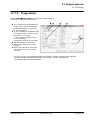
User Manual
AND Client
Version: IV/C
Author: Various
Document name: AND Client EN.pdf
This document contains 452 pages
Date of publication: 2013-10-01
All information in this manual has been included after careful review but is not deemed to be a warranty of product qualities.
AND Solution is liable only to the extent defined in the Conditions of Sale and Delivery.
Changes to the product in the service of technical progress are reserved.
AND
Advanced Network Design Copyright © 2011 AND Solution GmbH
Paintlib
Copyright © 1996-2002 Ulrich von Zadow and other contributors
LibTiff
Copyright © 1988-1997 Sam Leffler & © 1991-1997 Silicon Graphics, Inc.
LibSmi
Copyright © 1999-2002 Frank Strauss, Technical University of Braunschweig
Copyright © 1995-1999 Kungliga Tekniska Högskolan
(Royal Institute of Technology,Stockholm, Sweden)
All rights reserved.
DTL
Copyright © 2000 Michael Gradman and Corwin Joy
This maual is protected by copyright.
The manual and the software – wholly or in part – must not be reproduced, disseminated, altered or translated into any
other language or converted into any other format without the express prior written authorization of AND Solution.
© 2013 AND Solution GmbH, Munich, Germany
All rights reserved
AND® is a registered trademark
AND Solution GmbH
Karl-Schmid-Straße 14, 81829 München, Germany
Tel. +49 (89) 743533-0
Fax. +49 (89) 760 6020
Contents
Contents
Contents ...............................................................................................3
1
General information .................................................................8
1.1
Target group of this manual / required skills ............................................. 8
1.2
Components of the NDS documentation ...................................................... 9
1.3
Conventions .............................................................................................. 10
2
Fundamentals ........................................................................11
2.1
2.1.1
2.1.2
2.1.3
2.1.4
2.1.5
2.1.6
The AND program window and its elements ............................................. 12
Toolbars ......................................................................................................13
Output window .............................................................................................15
Status bar....................................................................................................15
Tool tips ......................................................................................................16
“Edit Object” window .....................................................................................16
Changing the window design ..........................................................................18
2.2
Dual-Monitor optimization ........................................................................ 20
2.3
Working with the mouse ........................................................................... 21
2.4
Working with the keyboard....................................................................... 23
2.5
Operating and drawing modes .................................................................. 25
2.6
Schematic and geo-schematic operating mode ......................................... 27
2.7
2.7.1
2.7.2
2.7.3
2.7.4
2.7.5
Navigating and zooming ........................................................................... 28
Navigating between documents ......................................................................28
Navigating between worksheets ......................................................................29
Navigating in worksheets ...............................................................................30
Navigating beyond document boundaries .........................................................31
Zooming ......................................................................................................31
2.8
Selecting objects ...................................................................................... 32
2.9
Locking objects ......................................................................................... 34
2.10
Moving objects.......................................................................................... 35
2.11
Copying objects ........................................................................................ 36
2.12
Deleting objects ........................................................................................ 37
2.13
Loading libraries for object selection ........................................................ 38
2.14
2.14.1
2.14.2
2.14.3
2.14.4
2.14.5
2.14.6
Network planning mode ............................................................................ 44
Plotting a component ....................................................................................44
Plotting a cable .............................................................................................48
Plotting other objects ....................................................................................52
Editing and changing cables ......................................................................... 113
Automatic labeling of objects........................................................................ 115
Dynamic Labels and Hierarchy Path .............................................................. 117
AND Client Manual IV/C
© AND Solution GmbH
Page 3 of 452
Contents
2.14.7
2.14.7.1.
2.14.7.2.
2.14.7.3.
2.14.7.4.
2.14.7.5.
2.14.8
2.14.9
Automatic numbering of objects ................................................................... 122
Setting the numbering format ...................................................................... 122
Rules of precedence .................................................................................... 123
Editing of the numbering settings from dialog................................................. 124
Counters in editing...................................................................................... 127
External counters........................................................................................ 128
Immediate editing of objects when plotting .................................................... 129
Design, drawing, and positioning assistance ................................................... 130
2.15
2.15.1
2.15.2
2.15.3
Optical connectors, optical connections .................................................. 141
Optical plug connections in the component editor ........................................... 141
Testing optical plug connections in AND ......................................................... 142
Attenuation of the optical connections ........................................................... 143
2.16
Creating a new document ....................................................................... 145
3
Automatic drawing mode .....................................................148
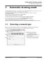
3.1
Selecting a network type ........................................................................ 148
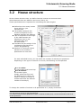
3.2
House structure ...................................................................................... 150
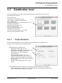
3.3
3.3.1
3.3.2
3.3.3
3.3.4
Distribution level .................................................................................... 151
Trunk structure .......................................................................................... 151
Levels ....................................................................................................... 152
Components ............................................................................................... 153
Options ..................................................................................................... 153
3.4
Generating a drawing ............................................................................. 154
3.5
Tap Optimization .................................................................................... 157
4
Civil works planning ............................................................159
4.1
Layers for trenches ................................................................................. 161
4.2
Plotting trench sections .......................................................................... 162
4.3
4.3.1
4.3.2
4.3.3
4.3.4
4.3.5
Laying cables in trenches ........................................................................ 163
Duplicating cables ....................................................................................... 164
Plotting cables in all directions ...................................................................... 164
Generating cables in all directions ................................................................. 165
Plotting dimensioning arrows ........................................................................ 165
Keyboard design assistance ......................................................................... 167
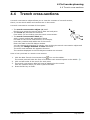
4.4
4.4.1
4.4.2
4.4.3
4.4.4
Trench cross-sections ............................................................................. 168
Twisting conduits in trenches ....................................................................... 170
Trench sections .......................................................................................... 171
Trench cross-section labeling ....................................................................... 172
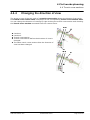
Changing the direction of view ..................................................................... 173
4.5
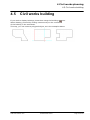
Civil works building ................................................................................ 174
5
Editing background files ......................................................175
5.1
5.1.1
5.1.2
5.1.3
5.1.4
5.1.5
Maps ....................................................................................................... 176
Loading a background map .......................................................................... 177
WMSClient Plugin ........................................................................................ 179
Scale and GIS coordinate system .................................................................. 184
Calculating cable lengths ............................................................................. 189
GIS and cluster planning ............................................................................. 191
AND Client Manual IV/C
© AND Solution GmbH
Page 4 of 452
Contents
5.1.6
Background editor ...................................................................................... 192
6
Project organization ............................................................198
6.1
Parent project organization .................................................................... 198
6.2
Organizing libraries ................................................................................ 201
6.3
6.3.1
6.3.2
6.3.3
6.3.4
Worksheets............................................................................................. 202
Creating worksheets ................................................................................... 203
Settings for worksheets ............................................................................... 208
Labeling of worksheet connections with the target address .............................. 212
Saving and loading worksheets ..................................................................... 215
6.4
6.4.1
6.4.2
6.4.3
6.4.4
6.4.5
Layers ..................................................................................................... 216
Defining layers globally ............................................................................... 216
Defining layers for worksheets ...................................................................... 217
Selecting and switching layers on and off ....................................................... 217
Deleting layers ........................................................................................... 218
Layer tips and usage options ........................................................................ 218
6.5
6.5.1
6.5.2
6.5.3
6.5.4
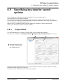
Specifying key data for search options ................................................... 219
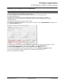
Project data ............................................................................................... 219
Installation numbers ................................................................................... 226
Locations ................................................................................................... 228
Sheet legends ............................................................................................ 231
6.6
Status ..................................................................................................... 233
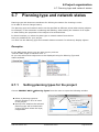
6.7
6.7.1
6.7.2
Planning type and network status .......................................................... 234
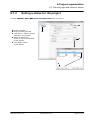
Setting planning types for the project ............................................................ 234
Setting a status for the project ..................................................................... 235
6.8
6.8.1
6.8.2
Independent Hotspots ............................................................................ 249
General information .................................................................................... 249
Application functional detailing ..................................................................... 250
7
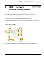
NIS – Network Information System .....................................281
7.1
7.1.1
7.1.2
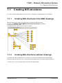
Creating NIS structures .......................................................................... 283
Creating NIS structures from AND drawings ................................................... 283
Creating NIS structures without drawings ...................................................... 283
7.2
7.2.1
7.2.2
7.2.3
7.2.4
7.2.5
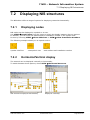
Displaying NIS structures ....................................................................... 284
Displaying nodes ........................................................................................ 284
Horizontal/Vertical display ........................................................................... 284
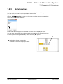
Service views ............................................................................................. 285
Remote powering view ................................................................................ 286
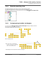
Compressing location rectangles ................................................................... 286
7.3
7.3.1
7.3.2
Navigating in NIS structures ................................................................... 287
Zooming NIS structures ............................................................................... 287
Moving image sections ................................................................................ 287
7.4
7.4.1
7.4.2
7.4.3
7.4.4
7.4.5
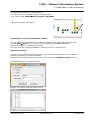
Editing the NIS network structure .......................................................... 289
Selecting nodes .......................................................................................... 289
Arranging network structure objects.............................................................. 290
Deleting nodes and links .............................................................................. 291
Editing project data ..................................................................................... 291
Deleting NIS projects .................................................................................. 291
AND Client Manual IV/C
© AND Solution GmbH
Page 5 of 452
Contents
8
Settings ...............................................................................292
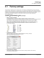
8.1
Factory settings ...................................................................................... 293
8.2
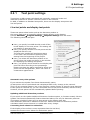
8.2.1
Project settings ...................................................................................... 295
Test point settings ...................................................................................... 296
8.3
8.3.1
8.3.2
8.3.3
8.3.4
8.3.5
8.3.6
Program settings .................................................................................... 299
Auto save .................................................................................................. 299
Setting program paths ................................................................................. 300
Setting line styles and display options ........................................................... 301
Setting user names ..................................................................................... 302
Setting the program language ...................................................................... 302
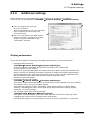
Additional settings ...................................................................................... 303
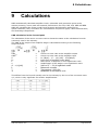
9
Calculations .........................................................................304
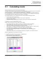
9.1
9.1.1
9.1.2
Calculating levels .................................................................................... 305
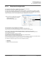
Possible reasons for level calculation failure ................................................... 306
Reversed components ................................................................................. 307
9.2
9.2.1
9.2.2
Amplifier settings ................................................................................... 308
Setting all amplifiers at once ........................................................................ 308
Setting individual amplifiers ......................................................................... 310
9.3
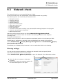
Network check ........................................................................................ 315
9.4
9.4.1
9.4.2
9.4.3
9.4.4
9.4.5
9.4.6
9.4.7
Return path calculation ........................................................................... 327
Editing upstream services ............................................................................ 328
Setting the return path transmitter ............................................................... 330
Setting the return path receiver .................................................................... 335
Setting the return path amplifier ................................................................... 336
Calculating the return path level at one point ................................................. 342
Blocking return paths for particular connections.............................................. 343
Return Path calculation as part of the network check ....................................... 344
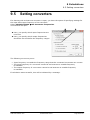
9.5
Setting converters .................................................................................. 348
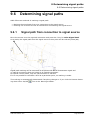
9.6
9.6.1
9.6.2
Determining signal paths ........................................................................ 349
Signal path from connection to signal source .................................................. 349
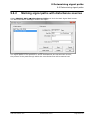
Marking signal paths with disturbance sources ................................................ 350
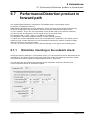
9.7
9.7.1
9.7.2
9.7.3
9.7.4
Performance/Distortion product in forward path ................................... 351
Distortion checking in the network check ....................................................... 351
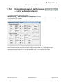
Calculating network performance – worst values in network ............................. 352
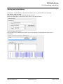
Distortion products at a selected point ........................................................... 353
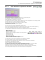
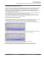
The distortion spectrum window ................................................................... 354
9.8
Information about the distortion product calculation ............................. 355
9.9
Calculating test points ............................................................................ 360
9.10
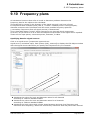
Frequency plans...................................................................................... 363
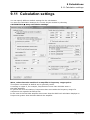
9.11
Calculation settings ................................................................................ 366
9.12
9.12.1
9.12.2
9.12.3
Calculation for optical Networks ............................................................. 371
Calculating optical output ............................................................................ 371
Optical disturbance calculation ..................................................................... 372
Splice Report and Splice/Patch List ............................................................... 373
9.13
9.13.1
9.13.2
Microducts .............................................................................................. 379
DuctPackage .............................................................................................. 379
Inhouse Microducts ..................................................................................... 389
AND Client Manual IV/C
© AND Solution GmbH
Page 6 of 452
Contents
9.13.3
9.13.4
Manhole (Schacht) ...................................................................................... 392
Trenches ................................................................................................... 397
9.14
9.14.1
9.14.2
9.14.3
9.14.4
9.14.5
9.14.6
9.14.7
9.14.8
9.14.9
9.14.10
Calculating remote powering .................................................................. 399
Starting the remote powering calculation ....................................................... 399
Remote powering calculation results ............................................................. 400
Remote powering basics in the libraries ......................................................... 400
Specifying remote power data in component editor ......................................... 401
Activating/Blocking connections for remote powering ...................................... 404
Remote powering calculation details .............................................................. 405
Remote powering outputs and error messages ............................................... 407
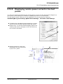
Displaying remote power current in live test points ......................................... 409
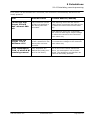
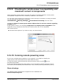
Checking for remote power incompatibility and maximum current in components410
Coloring remote powering areas ................................................................... 410
10
Bills of Materials ..................................................................411
10.1
Creating a Bill of Materials ...................................................................... 411
10.2
Editing bills of materials ......................................................................... 413
10.3
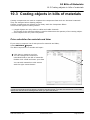
Costing objects in bills of materials ........................................................ 415
11
Output options .....................................................................417
11.1
11.1.1
11.1.2
11.1.3
11.1.4
11.1.5
11.1.6
Printing ................................................................................................... 417
Printing test point lists ................................................................................. 417
Printing network structures .......................................................................... 419
Printing connector lists ................................................................................ 419
Printing drawings, drawing sections or blocks ................................................. 420
Printing splice boxes ................................................................................... 421
Page setup ................................................................................................. 422
11.2
11.2.1
11.2.2
11.2.3
11.2.4
11.2.5
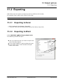
Exporting ................................................................................................ 423
Exporting to Excel ....................................................................................... 423
Exporting to Word ....................................................................................... 423
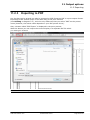
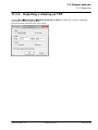
Exporting to PDF ......................................................................................... 424
Exporting a drawing as TIFF ......................................................................... 425
Exporting a drawing as a DXF ....................................................................... 426
11.3
Reports ................................................................................................... 427
11.4
11.4.1
11.4.2
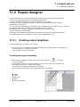
Report designer ...................................................................................... 432
Creating report templates ............................................................................ 432
Variables in AND ......................................................................................... 439
12
Automation interface of the client .......................................444
Index
446
Glossary (see Separate Manual) ......................................................452
AND Client Manual IV/C
© AND Solution GmbH
Page 7 of 452
1 General information
1.1 Target group of this manual / required skills
1
General information
Advanced Network Design – AND, for short – is a software package for the planning,
documentation, and calculation of antenna, CATV, SAT, und HFC systems.
You can create a complete network plan, from the headend to the subscriber outlet,
using simple drag-and-drop plotting of symbols taken from comprehensive
component libraries.
The drawing can be executed directly within the site plan or topographical map in schematic or
geo-schematic form.
You can set all system parameters manually or automatically using user-friendly functionality
and clearly laid out windows.
AND can also: interpret your drawing; calculate amplification levels, subscriber and connection
point levels, return paths and network performance (CTB, CSO, C/N, MER, BER) for any grid;
notify you of all required plug connections; and create bills of materials with costs and
assembly times.
1.1
Target group of this manual /
required skills
The target group of this manual is all users of the AND software.
Readers are assumed to be familiar with using personal computers and
the Window operating system. No skills in operating CAD programs are required.
AND Client Manual IV/C
© AND Solution GmbH
Page 8 of 452
1 General information
1.2 Components of the NDS documentation
1.2
Components of the NDS
documentation
The documentation of the NDS software is structure into two groups:
1. User documentation
2. Administrator documentation
The user documentation comprises the manuals






AND 4.1
GisArea (incl. „Design Alternatives“)
LibEdit
WebInfo
ViewToGo
Glossary + List of shortcuts
The administrator documentation comprises the parts
 Installation
 Maintenance
AND Client Manual IV/C
© AND Solution GmbH
Page 9 of 452
1 General information
1.3 Conventions
1.3
Conventions
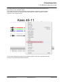
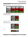
This manual contains the description of all available versions of AND,
that is, LocalArea, COAX, and FIBRECOAX. Not all functions are available in all versions.
If a function is only available for certain versions, this will be indicated accordingly.
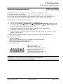
Pay attention to the following figure:
If a function is only available in certain license versions, this is indicated by a checkmark.
The abbreviations stand for:
LocalArea
COAX
FibreCoax
=
=
=
AND LOCAL Version
AND COAX Version
AND HFC Version
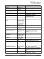
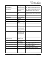
In addition to the above, in this manual, the following typographical conventions also apply:
Menu commands
These are printed in bold and italic type.
The menu name is additionally written in upper case laters.
The “Toolbars” command in the “View” menu
is show as follows for example:
VIEW  Toolbars
Window names,
tab names and
window contents
The names of windows and their contents
are printed in italics:
Window System data.
Buttons
A button is a visual element in a dialog box used
to trigger a function.
Examples:
Shift key
This is the key for switching between upper and
lower case letters
Examples:
The examples given in the individual sections are based on fictional data.
AND Client Manual IV/C
© AND Solution GmbH
Page 10 of 452
2 Fundamentals
2
Fundamentals
This chapter will familiarize you with the basic functions and
methods used to plot a network plan and work in AND.
The chapter provides information about










the AND program window and its elements,
working with two monitors (dual-monitor optimization),
working with the mouse and keyboard
the operating and drawing modes in AND,
the schematic and geo-schematic operating modes,
the navigating and zooming,
manipulating objects,
loading libraries for object selection,
network planning drawing mode
creating a new document.
AND Client Manual IV/C
© AND Solution GmbH
Page 11 of 452
2 Fundamentals
2.1 The AND program window and its elements
2.1
The AND program window and its
elements
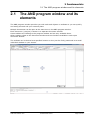
The AND program window provides you with tools and objects on toolbars so you can quickly
and easily plot and edit your network plans.
Multiple documents can be open at the same time in the AND program window.
Each document (=project) is shown in a separate document window.
Some toolbars are relating to the program window and are only available there.
Other toolbars relate to the document window and are therefore available in each open
document window.
The toolbars can be docked at a specified location or they can be freely positioned as a small
individual window on your screen.
AND Client Manual IV/C
© AND Solution GmbH
Page 12 of 452
2 Fundamentals
2.1 The AND program window and its elements
2.1.1
Toolbars
Commands and functions that you use on a regular basis are available as icons in the toolbars.
The commands are grouped into functional blocks and placed in various toolbars.
Use the VIEW  Toolbars command to switch toolbars on or off.
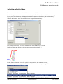
Toolbars can be either docked, for example, in a position near the window edge,
or freely positioned (floated) anywhere on your screen.
To position a toolbar, drag it by the “move handle” () or
double-click it and then drag the window by the title bar ().


Freely positioned or floating toolbar
Docked toolbar
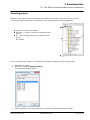
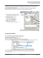
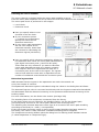
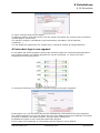
The object selection window is a special form of the toolbar.
It displays icons and components from libraries and makes them available for use in drawings.
Object section window in the list view (left) and tree view (right)
There is one such window per document window and each displays the components available
in the libraries for that particular document.
To plot a component into the network plan,
drag it from the object selection window and position it on the worksheet.
Depending on the setting, the window shows the objects and components of a single library,
of all libraries, or of a user-defined selection of objects and components.
Using the Show as List, Show as Tree, or Find Symbol tabs,
you can switch between the list, tree and quick search views.
You will find more information in the Loading Libraries for Object Selection section
(see Page 38).
AND Client Manual IV/C
© AND Solution GmbH
Page 13 of 452
2 Fundamentals
2.1 The AND program window and its elements
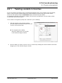
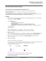
Selecting groups
Objects in the object selection window are divided into groups in the tree view to provide
a clear overview of the library. All objects in the same group are interchangeable.

 Groups are shown as folders
 Click the (+) sign to show the contents of the
group
 A (-) sign indicates that the contents of this
group
are visible


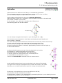
This is to exchange an object in a drawing with another object from the same group:
1.
2.
Selection an object.
Press the G key for Replace Group.
The following window opens:
3.
Click the object in the drawing that you wish to exchange and then click OK.
AND Client Manual IV/C
© AND Solution GmbH
Page 14 of 452
2 Fundamentals
2.1 The AND program window and its elements
2.1.2
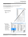
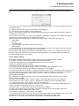
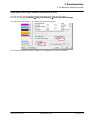
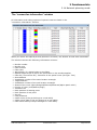
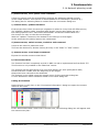
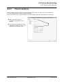
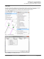
Output window
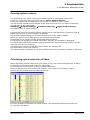
The output window displays notifications, warnings and error messages.
It can be docked on the left, right, top or bottom of the program window, or freely positioned.
Use VIEW  Messages to switch the output window on and off.
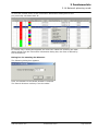
In this picture you see a list of warnings that occurred during a network check.
If you click an entry in the output window, the associated component will appear red and
blinking in the document window.
If you simultaneously press the Shift button,
the Auto Zoom function will be switched off, that is, the zoom level will not change.
Use the context menu to copy the content in the output window into a text file or
to the clipboard.
Use the CALCULATION  Warnings  Delete All Warnings command to clear the window.
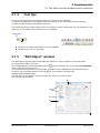
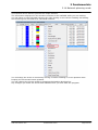
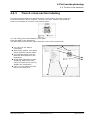
2.1.3
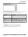
Status bar
The status bar displays information about the edit status of the open project and
which functions or modes are active.














Active mode
Object to be positioned
Object selected under the cursor
Sheet number
Current X-coordinate
Current Y-coordinate
Snap function activated/deactivated
AND Client Manual IV/C
© AND Solution GmbH
Page 15 of 452
2 Fundamentals
2.1 The AND program window and its elements
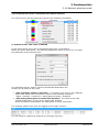
2.1.4
Tool tips
If you pause with the mouse pointer above the icons on the toolbars,
or above a component in the object selection window or the worksheet without clicking,
a small window (tooltip) will appear with text.
This window tells you what function the icon triggers, which component the icon displays in the
drawing, or the library from which the icon originates.

 Tooltip for a component drawn on the worksheet
 Tooltip for an icon on a toolbar
2.1.5
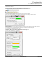
“Edit Object” window
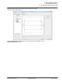
The Edit Object window opens automatically when you click an object in the worksheet
(a component, cable, text, etc.).
For worksheets and worksheet attachments
, press the Enter key or choose the Properties
option from the context menu.
The content of the window is dynamically generated and is adapted to the selected object.
As there is a lot of data relating to each object, the window is divided into
multiple sub-windows (tabs).
The left side of the window shows the tab tree, which you use to open
the various sub-windows.





AND Client Manual IV/C
© AND Solution GmbH
Page 16 of 452
2 Fundamentals
2.1 The AND program window and its elements
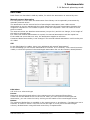
 Sub-windows appearing
as tabs.
 Drag this sizing handle
to resize the window.
The size will remain as
you set it.
 Tab tree for switching
tabs.
 Click the second level to
display the corresponding
information in the tab
window on the right.
 The first level shows the
type
of information on each
tab.
AND Client Manual IV/C
© AND Solution GmbH
Page 17 of 452
2 Fundamentals
2.1 The AND program window and its elements
Sub-Window for editing
You can also open the individual sub-windows of the Edit object window directly with a hot key
or with the context menu:
Dynamic data
This sub-window opens automatically when you click the object.
Component information
You can call this sub-window directly by pressing the I key for the object or choosing the
Component information item from the context menu.
For an object originating from a library, the Basic Data No. 1 tab will open.
Location information/Installation number
You can call this sub-window directly by pressing the O key for the object or
choosing the Edit Location item from the context menu.
This is where you create the installation and serial numbers as well as the location.
Color / Layer information
You can call this sub-window directly by pressing the F key for the object or
choosing the Color/Layer item from the context menu.
This is where you edit the color of the active object and its assignment to a layer.
URL
You cannot open this sub-window directly.
You have to call the associated tab once the Edit Object window has already been opened.
Here, you can enter a link to the object.
The link can refer to a file in the file system or to a site on the in the intranet or
on the Internet.
Note: If you activate the Open with Mouse Click option, the link will automatically open when the object is
clicked. After that, you can only access the editing window by clicking the Properties item in the context
menu.
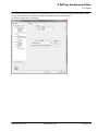
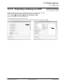
2.1.6
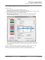
Changing the window design
You can change the design of the program window to suit your taste.
The program provides a number of designs among which you can choose the design
you like best.
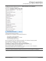
At the time of writing this manual, the following designs are available
AND Client Manual IV/C
© AND Solution GmbH
Page 18 of 452
2 Fundamentals
2.1 The AND program window and its elements
Flat (simple)
Flat
3D design (blue)
3D design (silver)
Modern (blue)
Modern (black)
Modern (aqua)
Modern (silver)
To change the window design, choose VIEW  Change Design and
then choose one of the designs listed:
The design you choose does not affect the functions of the program; it only concerns the appearance of the
program window (exception: remote sessions. In this case, some designs may result in performance problems). For this reason, you can change the window design again at any time.
AND Client Manual IV/C
© AND Solution GmbH
Page 19 of 452
2 Fundamentals
2.2 Dual-Monitor optimization
2.2
Dual-Monitor optimization
NDS features full dual-monitor capability in a local installation.
To enable the best possible use of a second monitor, you can move all toolbars and
other ‘docked’ window onto a second monitor.
This enlarges the pure worksheet space on the NDS and provides clear separation
between the worksheet and tools.
Under Citrix, this dual-monitor capability is only possible to a limited extent:
If NDS is executed in a 'Seamless Window,' both the main window and all toolbars
can be positioned on the primary monitor only.
You can also start NDS in a surrounding window whose maximum (absolute) size depends
on settings and the available resources of the Citrix server.
In this way, depending on the settings, it is possible to create a window that can be enlarged
beyond the primary monitor of the Citrix client.
The NDS main window and the toolbars can be positioned anywhere within this window.
AND Client Manual IV/C
© AND Solution GmbH
Page 20 of 452
2 Fundamentals
2.3 Working with the mouse
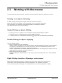
2.3
Working with the mouse
A mouse with two buttons and a wheel is recommended for optimum efficiency in AND.
Pointing to an object = Selecting
In AND, simply pointing at an object with the mouse is an action.
When you point to an object in the worksheet you are actually selecting it.
The next action you perform using the keyboard, for example, deletion,
will apply directly to the selected object.
Single-Clicking an object = Editing
 Clicking once on an object in the worksheet opens the Edit Object window.
 Clicking once on a component that has ist own worksheet,
 or clicking once on a worksheet connection
, opens the corresponding worksheet.
Double-Clicking an object = Applying
Use the double-click to
 Plot a component in the worksheet:
Double-clicking an object in the object selection window applies the object in the drawing.
The object is now attached to the mouse pointer, which is automatically located in the
middle of the sheet. From there, position the object.
(This is an alternative to holding down the mouse button and dragging the object from the
object selection window onto the worksheet.)
 Select a layer for future objects:
Double-clicking the desired layer on the Layer and Color toolbar sets it for future plotted
objects.
Right-Clicking a location = Opening a context menu
Right-clicking with the mouse on a location on the screen opens the context menu.
This means: the commands and functions possible at this location are shown.
This is a quicker way of carrying out command and is used very frequently in AND.
AND Client Manual IV/C
© AND Solution GmbH
Page 21 of 452
2 Fundamentals
2.3 Working with the mouse
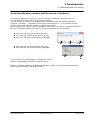
Answering the query window with the mouse or keyboard
The program displays a window for various functions to wait for a decision from you.
This window can contain two or three answer buttons.
You can answer by clicking the appropriate answer button with the left mouse button.
However, it is faster – regardless of where the mouse pointer is – if you simply click the
desired answer with the left, middle, or right mouse button.
If you would rather answer using the keyboard, the left mouse button is represented by the
Esc key, the middle button by the N key and the right button by the spacebar.
 Click with the left mouse button (Esc key)
 Click with the middle mouse button (N key)
 Click with the right mouse button (spacebar)



 Click with the left mouse button (Esc key)
 Click with the right mouse button (spacebar)



This functions are only available if the program is set to
“AND 3.2 compatible keyboard and mouse inputs”:
Options  Program Settings  Additional Settings  AND 3.2 Compatible Keyboard and
Mouse Inputs activated (checkmark visible).
AND Client Manual IV/C
© AND Solution GmbH
Page 22 of 452
2 Fundamentals
2.4 Working with the keyboard
2.4
Working with the keyboard
You will work significantly faster in AND if you familiarize yourself with the keyboard functions.
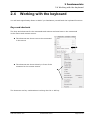
Keys and shortcuts
The keys and shortcuts for the commands and actions are listed next to the commands
in the menus and context menus.
 The shortcuts are shown next to the command
in the menus

 The shortcuts are shown directly in front of the
command in the context menus.

The shortcuts are key combinations involving the Ctrl or Alt key.
AND Client Manual IV/C
© AND Solution GmbH
Page 23 of 452
2 Fundamentals
2.4 Working with the keyboard
Arrow buttons
The arrow buttons on the keyboard simulate the mouse movements.
Each time you press the key, the mouse pointer (white arrow) will move a certain set distance
in the direction of the key pressed.
If you additionally hold down the Alt key, the mouse pointer will move with pixel precision.
Spacebar
The spacebar simulates the right mouse button.
Because it makes a difference when working with the mouse whether the mouse button is held
down or released, holding down the spacebar simulates one of these actions - either holding
down the left mouse button or releasing it.
More complex actions involving holding down or releasing the mouse, can also be performed
using the keyboard. Here is an example of block selection (see Page 33): Move the mouse
pointer with the arrow buttons to the upper left corner of the desired area; press the spacebar
once; move the mouse pointer with the arrow buttons to the lower right corner of the desired
area and press the spacebar once again.
Backspace key
The backspace key simulates the right mouse button. Use it to open the context menu.
AND Client Manual IV/C
© AND Solution GmbH
Page 24 of 452
2 Fundamentals
2.5 Operating and drawing modes
2.5
Operating and drawing modes
There are three operating modes in AND.
You can easily tell which mode is active by the appearance of the mouse pointer.
The operating mode automatically changes according to the action that you are carrying out.
Standard mode
You are in standard mode by default.
In this mode, you can call menu commands, select objects from a library or
the worksheet, zoom the worksheet, or select another sheet.
You can recognize standard mode by the white arrow shape of the mouse pointer.
Shape of the mouse pointer in standard mode:
Positioning mode
You are positioning mode after you have seleced an object from the library and
are plotting it on the worksheet, or after you have selected an object on the worksheet and
are moving it.
You can recognize positioning mode by the black cross shape of the mouse pointer.
Crosshairs comprising a vertical and a horizonal line (light blue) and the selected icon (violet)
are also attached to the pointer.
Shape of the mouse pointer in positioning mode:
Block mode
You will be in block mode after you have selected more than one object on the worksheet.
Any subsequent actions then apply to the whole block of selected objects.
The dashed border shows the objects in the block:
On the status bar, you can see whether you are in standard, positioning, or block mode.
In positioning mode, it will also specify details about the objects you are positioning:
The following drawing modes are distinguished:





Network planning
Civil works planning
Background arranging
View setting (in the GIS Area module only)
Tile editing (in the GIS Area module only)
AND Client Manual IV/C
© AND Solution GmbH
Page 25 of 452
2 Fundamentals
2.5 Operating and drawing modes
You must actively change the drawing mode by opening the drop-down list box on the toolbar
next to Drawing mode and selecting the desired mode.
A detailed description of plotting network plans in Network planning mode is provided
in the Network Planning Drawing Mode chapter (see Page 44).
A detailed description of civil works mode is provided in the Civil Works Planning chapter
(see Page 159).
A detailed description of how to edit background files is provided in the Editing Background
files chapter (see Page 175).
A detailed description of how to divide a plan into multiple tiles and thus into multiple files is
provided in the “Editing Tiles” section in the GIS Area Manual.
AND Client Manual IV/C
© AND Solution GmbH
Page 26 of 452
2 Fundamentals
2.6 Schematic and geo-schematic operating mode
2.6
Schematic and geo-schematic
operating mode
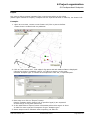
In schematic operating mode, also known as orthogonal mode, only vertical and horizontal
cables are shown, and compoents can only be rotated through 90° angles.
You will automatically be in schematic operating mode when you create a new document and
do not load a map or graphic as the background.
As from version AND COAX, background maps (see Chapter 5) can be edited.
The purpose of this feature is to plot the network plan according to the site plan,
that is, geo-referenced.
A background map can be a site plan or a topographic map or a story floor plan of a building.
If an AND Smart Server is connected with GIS, maps can be provided through this server.
As soon as you have loaded a back ground map using
FILE  Background with Load Bitmap Background or Load DXF Background,
you will automatically be in geo-schematic operating mode.
Now you will be plotting the network plan based on a topographical map.
You will thus be able freely to rotate components, cables and trenches in a non-orthogonal
way, that is, according to the site plan.
The advantage here is, in addition to the electrical network information (schematic portion),
you simultaneously have relatively accurate documentation of the site in the plan.
Also, the cable lengths will be drawn automatically from the scale –
which of course significantly speeds up your work.
To avoid the advantages of the geo-schematic operating mode resulting in unclear diagrams
in complex or extensive projects, AND allows you to create multiple worksheets.
In this case, separate diagrams are encapsulated in an icon in the site plan –
simply click the icon to call up the worksheet.
You will automatically switch to the geo-schematic operating mode when you have loaded
a background (graphics in dfx or bitmap format).
Use the
icon or the F8 key on the Design Assistance
toolbar
to switch freely between schematic (orthogonal) and geo-schematic operating modes.
AND Client Manual IV/C
© AND Solution GmbH
Page 27 of 452
2 Fundamentals
2.7 Navigating and zooming
2.7
Navigating and zooming
If you are dealing with a complex AND project, you can create a clearer overview
of the network plan if you divide it into multiple worksheets.
When working with documents (=projects) and worksheets, you may be jumping from sheet
to sheet or having to zoom in or out to achieve the desired ease of use.
That means you need assistance with navigating (=paging) through the documents and
worksheets and zooming (=enlarging or reducing) in the worksheet views.
2.7.1
Navigating between documents
You have two options for switching between multiple open documents (= projects):
 On the Projects and Sheets toolbar, choose the desired project from the list
next to Project.
 Click the desired project name in the Window menu.
Alternatively, you can use the shortcut Ctrl-Tab.
AND Client Manual IV/C
© AND Solution GmbH
Page 28 of 452
2 Fundamentals
2.7 Navigating and zooming
2.7.2
Navigating between worksheets
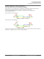
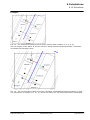
To switch between different worksheets in a document, you have the following options:
Click the worksheet icon in the active document
(= a component for which a sub-worksheet has been created) or click its connection.

 You can recognize a worksheet icon by
the dashed border around the icon.
 Click the connection to open the sub-worksheet
 Click the worksheet icon to open the sub-worksheet


The associated worksheet will open.
The section of the image is set to appear in the middle of the screen.
Click the worksheet connection
in the sub-worksheet to switch back to the parent document.
If you are in the sub-worksheet, use the S key or the Exit Worksheet function
in the context menu to return to the parent worksheet.
Press the Page  or Page  buttons to switch to the previous or next worksheet.
These buttons are also available when positioning components.
If, for example, you want to copy a block into another worksheet,
you can access the desired sheet using these buttons.
If you cannot switch sheets, an audible notification signal will sound.
For example, if you want to copy a non-orthogonal object from a site plan into a
schematic plan, you cannot switch from the worksheet with the site plan to the worksheet
with the schematic plan.
On the Projects and Sheets toolbar, choose the desired worksheet from the list
next to Worksheet.
AND Client Manual IV/C
© AND Solution GmbH
Page 29 of 452
2 Fundamentals
2.7 Navigating and zooming
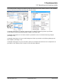
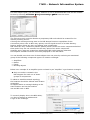
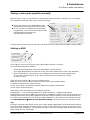
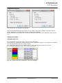
Settings for the worksheet preview
You can make display settings for worksheets that appear in a drawing and
that reference a sub-worksheet.
To open the settings window, choose the Properties item from the context menu
for the worksheet icon or click the worksheet icon while holding down the Alt key.
The Edit Object window will open.
Here, you will find the Display box where you can choose a preview type from
the various types available:
Example of various preview types:




Worksheet preview: No preview ( ), low (), medium (), and high () quality.
Note: The worksheet preview functions recursively when set to high quality, that is,
the preview of a worksheet also appears in the preview of the parent worksheet.
Depending on the nesting level, this can result in slower loading times.
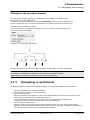
2.7.3
Navigating in worksheets
Navigating within a worksheet is called scrolling. You have the following scroll options:
 Use the horizontal and vertical scrollbars.
 Use the mouse wheel for vertical scrolling.
 Use the pan function:
Hold the middle mouse button or the mouse wheel down and move the mouse over the
edge of the worksheet. The worksheet will move.
If you additionally hold the Alt key down, the movement will be speeded up,
enabling you to move further with fewer mouse movements.
 Use the right mouse button:
Hold the right mouse button down and move the mouse over the edge of the visible
worksheet. The worksheet section moves about half of the width or height of the window.
The mouse pointer is then in the middle of the window.
AND Client Manual IV/C
© AND Solution GmbH
Page 30 of 452
2 Fundamentals
2.7 Navigating and zooming
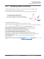
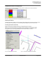
2.7.4
Navigating beyond document boundaries
For very large projects, the drawings are often divided into multiple documents.
In this case, the individual projects can be saved using the
PROJECT DATA  Project and Sheet Data  Save Worksheet command and
linked with the Load Worksheet command from the context menu.
The program thus automatically generates entry and exit points.
These points then become the navigation points.
This function is available when using the AND Smart Server or AND FIBRECOAX version.
You will find more information about this in the
“Entry and Exit Points" chapter in the “AND GIS Area” Manual.
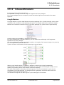
2.7.5
Zooming
AND provides different ways of zooming a drawing in or out.
 Move the mouse pointer to the location you are interested in and
press the + key or the - key to enlarge or reduce the worksheet view.
 Move the mouse pointer to the location you are interested in and
press the SHIFT key + left/right mouse key.
With every press of the Tab key, you switch between the detail, medium,
and overview zoom levels.
You can also choose these zoom levels using the context menu.
 On the toolbar next to the zoom icon
,
open the list of zoom options and choose the desired level.
After that, you can change the view size with every click of the zoom icon.
Use Zoom In or Out to incrementally enlarge or reduce the view.
To use Zoom Rectangle, you have to place a box around the area you wish to enlarge.
To do this, click the upper left or lower right corners.
Use Zoom All to show the entire worksheet (including legend).
Use Zoom Borders to reduce the worksheet so that all components are visible in the workksheet (without legend).
 Use the scale setting options on the Projects and Sheets toolbar to change the scale
.
The drawing will then be scaled to your desired setting (enlarged or reduced).
AND Client Manual IV/C
© AND Solution GmbH
Page 31 of 452
2 Fundamentals
2.8 Selecting objects
2.8
Selecting objects
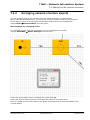
To edit an object in a worksheet (move, delete, rotate, etc.), you must first select it.
Select objects (components, cables, texts, marker lines, trench elements)
by moving the mouse pointer over them.
Selected objects will change color:
 A selected object will be shown in purple.
 A selected worksheet connection is shown in red.
 Objects linked to the currently selected object
(e.g. associated texts, test point windows) are shown in blue.
Only one object can be selected at a time
(together with those objects that are linked to the selected object).
When multiple objects overlap each other and you move the mouse over them,
the topmost object is selected.
If you wish to select an object on a lower layer, press the Shift key to switch
to the next object.
The colors stated are standard colors and can be defined in the Line Styles and
Display Options menu (see Page 301).
AND Client Manual IV/C
© AND Solution GmbH
Page 32 of 452
2 Fundamentals
2.8 Selecting objects
Selecting blocks
If more than one object is selected at once, that is called a block.
The objects in a block are contained within a marker rectangle bordered by a dashed line.
When you move the mouse pointer over the box, all objects in the block will be displayed blue.
You have the following options for selecting blocks:
 Exact selection with a marker rectangle
Hold the left mouse button down and drag a box from the upper left to the lower right
in your worksheet. All objects that are completely within the box will be shown blue.
This means that they belong to the selected block.
After the box has been moved, the objects will be displayed black again and the border of
the block will be displayed with a dashed line.
As soon as the mouse pointer is again moved over the block,
the objects and the border lines will be shown blue again.
 Approximate selection with a marker rectangle
Hold the left mouse button down and drag a box from the lower right to the upper left
in your worksheet. All objects that you touch (they do not have to be completely within
the marker rectangle) will be shown blue. This means that they belong to the selected
block and are selected.
After the box has been moved, the objects will be displayed black again and the border of
the block will be displayed with a dashed line.
As soon as the mouse pointer is again moved over the block, the objects and the border
lines will be shown blue again.
 Using the Ctrl key
Hold down the Ctrl key and click one after the other on the objects you wish to select.
 The objects will be displayed blue. At the same time, a dashed-line block will appear.
Use the Ctrl key to enlarge or reduce the number of elements in a block that has already
been created:
Hold down the Ctrl key and click an object in the block to remove it from the selection.
You can enlarge the block by pressing the Ctrl key and dragging open a new marker rectangle. The objects within the border will expand the already existing block.
 Using a menu command
Choose EDIT  Select All to select all (non-locked) objects in the worksheet.
To move, position, or rotate a block, proceed as with individual objects.
You will find a description of the block copying function in the “GIS Area” Manual (see Section 1.2).
AND Client Manual IV/C
© AND Solution GmbH
Page 33 of 452
2 Fundamentals
2.9 Locking objects
2.9
Locking objects
If you wish to avoid moving and editing objects unintentionally, lock them.
This is particularly helpful for bitmaps, OLE objects, lists, etc.
To lock an object, select it.
Then choose the Lock Object command from the context menu.
The objects can no longer be selected or edited.
If you wish to unlock an object, choose PROJECT DATA  Unlock All Locked Objects.
(Objects can also be unlocked individually using the context menu.)
AND Client Manual IV/C
© AND Solution GmbH
Page 34 of 452
2 Fundamentals
2.10 Moving objects
2.10 Moving objects
To move an object to another location on the worksheet, use the mouse or the keyboard.
Object groups
Objects/components form a group with their label text.
By switching the group function on or off, or selecting a certain group object,
you can determine whether the whole group will be moved or just an individual object.
Switch the group function on or off using the Move/Copy Object Groups icon.
(<G> im Positioning Mode)
on the standard toolbar.
You can also use the G key to switch the group function on or off while moving the object.
After starting AND, the group function is typically on.
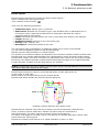
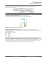
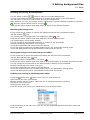
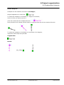
The objects in a group have a specific hierarchical relationship to one another.
For components, the component has priority 1 and the accompanying text, priorty 2.
For test points, the test point itself () has priority 1;
the test point window (), priority 2 and
the accompanying text (), priority 3.



If you select a priority 1 element to move, and the group function is active,
all elements in that group will be moved.
If you select a low priority element (2 or 3), only that element will move and
possibly any subordinate elements, irrespective of whether the group function is active or not.
AND Client Manual IV/C
© AND Solution GmbH
Page 35 of 452
2 Fundamentals
2.11 Copying objects
2.11 Copying objects
You can copy objects by selecting them, holding down the Ctrl key and
dragging them to the desired position.
When working with the keyboard, select the object you wish to copy and
press the N key for Copy Object. Now you can position the copied object.
Copying using the mouse
Select the object by moving the mouse pointer over it and drag it to the desired position
while holding down the left mouse button.
While you position the object, you can rotate it in 90° increments by pressing the R key,
or you can snap it to another object using the F key (see also Snapping, Page 132).
If you are working in geo-schematics, you can also rotate the object in 1° or 2° increments
with the S and D keys.
Copying using the keyboard
Select the object by moving the mouse over it.
Press the B key to activate the moving mode.
Move the object in the desired direction with the arrow keys.
Press the spacebar to deactivate the moving mode.
While you position the object, you can rotate it in 90° increments by pressing the R key,
or you can snap it to another object using the F key (see also Snapping, Page 132).
If are working in geo-schematics, you can also rotate the object in 1° or 2° increments
with the S and D keys.
AND Client Manual IV/C
© AND Solution GmbH
Page 36 of 452
2 Fundamentals
2.12 Deleting objects
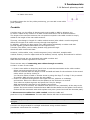
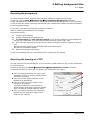
2.12 Deleting objects
Delete objects by selecting them and pressing the Del key (delete). Now the selected object
will blink red and a query window will open, asking you whether you really want to delete the
object. Confirm the deletion.
AND Client Manual IV/C
© AND Solution GmbH
Page 37 of 452
2 Fundamentals
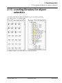
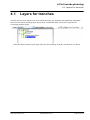
2.13 Loading libraries for object selection
2.13 Loading libraries for object
selection
The object selection window is available to you for selecting objects
you wish to plot in a network plan.
To display objects, you must load one or more libraries.
AND Client Manual IV/C
© AND Solution GmbH
Page 38 of 452
2 Fundamentals
2.13 Loading libraries for object selection
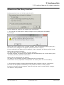
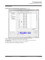
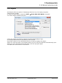
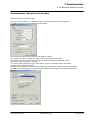
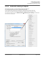
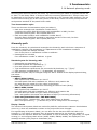
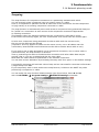
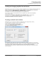
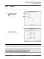
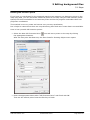
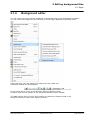
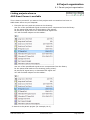
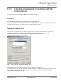
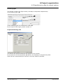
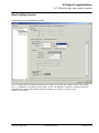
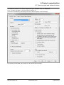
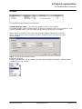
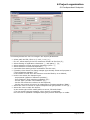
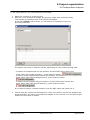
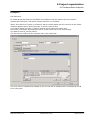
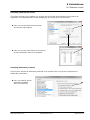
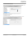
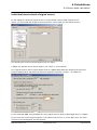
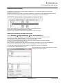
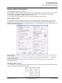
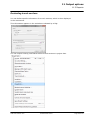
Editing the libraries list
Before you begin plotting objects, create a list of all the libraries from which
you would like to select objects.
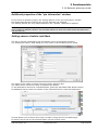
Click with the right mouse button in the object selection window and
choose the Edit Library List command.
The libraries window will open:

 Click here to select the libraries that you wish to
use in your network plan
and
load into the local
memory.

 Only ever use
the preset path.
Only the library
name will be saved
in the drawing files,
not the path.
If you wish to load
a library from a path
other than the present path, AND
many not find it
once you have reloaded the drawing.


Select the libraries () and load them in this way ().
AND Client Manual IV/C
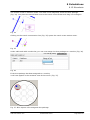
© AND Solution GmbH
Page 39 of 452
2 Fundamentals
2.13 Loading libraries for object selection
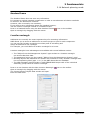
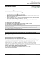
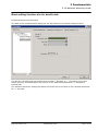
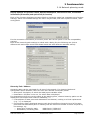
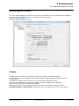
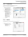
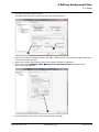
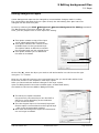
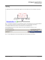
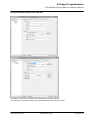
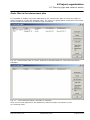
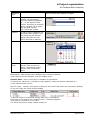
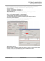
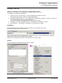
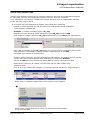
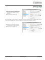
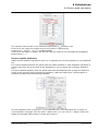
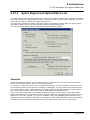
Extensions of the library functions
Implemented as from 4.0.765.61 and 4.2.847.0
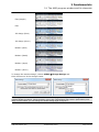
Library dialog box with the new options with a red border
1. You can set for what type of library changes a query dialog box will appear,
for example:
Option On Every Change: Even on small changes, such as component name, price, etc.,
the above query dialog box will appear (without the word "major").
If Yes is selected, the library will be replaced; if No is selected, the library will be linked.
Option Only on Major Changes:
The above dialog box only appears on major changes.
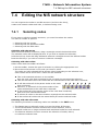
On small changes, the library in the drawing will be replaced by the current library from
the library directory without confirmation.
Option Only If Components Are Missing:
The library in the drawing is always replaced by the current library.
Confirmation is only requested if components are missing from the current library.
2. If the option Update Crosstexts Automatically After Loading A Library is activated,
the texts will be updated immediately if they show the data of a library object.
In previous versions of the program, that was only the case for major library changes.
The option is on by default.
AND Client Manual IV/C
© AND Solution GmbH
Page 40 of 452
2 Fundamentals
2.13 Loading libraries for object selection
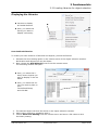
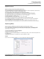
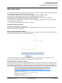
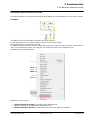
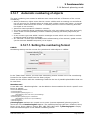
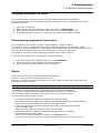
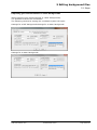
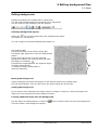
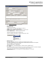
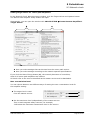
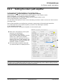
Displaying the Libraries
 Use this to display
all loaded libraries.




 Here, you select the
library you want to
display exclusively.
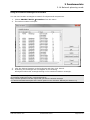
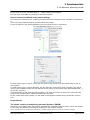
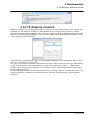
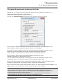
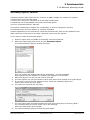
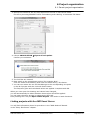
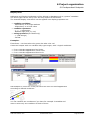
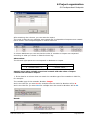
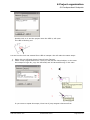
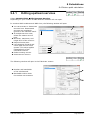
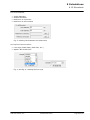
User-Defined Libraries
To create your own selection of libraries and objects, proceed as follows:
1.
2.
Activate the User Setting option in the context menu of the object selection window.
No libraries and objects will now be shown.
Now, choose the Add Object(s) item from the context menu.
The following window will open:

 Here, you select the library whose objects you
wish to display in the list
below.
 Here, you select the object you wish to place in
your
use-defined library
and click OK.
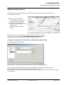
3.
4.
5.

The selected object will then be shown in the object selection window.
Select other objects by repeating step 2.
Choose Save User Setting from the context menu and enter a file name to save
the library setting.
AND Client Manual IV/C
© AND Solution GmbH
Page 41 of 452
2 Fundamentals
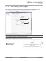
2.13 Loading libraries for object selection
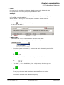
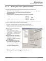
Linking libraries
Linking means that the library information actually saved in the library files
is also deposited in the drawing file.
This is only done for components that are in use
(one exception are all connectors and all amplifier assembly components).
This guarantees the integrity of the drawing even without library files if, for example,
they are to be archived or sent via e-mail.
Use the Link Status button to switch the link status of an individual library in relation
to the active drawing project.
The requirement for changing the link status from "linked" (connected) to "external" (normal)
is the existence of the library in the defined library directory.
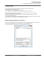
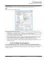
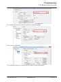
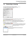
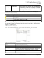
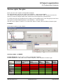
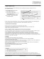
Replacing missing objects in the library
If one or more libraries have been changed such that components are completely missing or
have become incompatible, you can correct this on the component level.
Click the Missing Objects button and the following window will open.
AND Client Manual IV/C
© AND Solution GmbH
Page 42 of 452
2 Fundamentals
2.13 Loading libraries for object selection
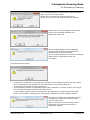
If icon graphics of a library have been modified during the processing time,
the change will only be applied after the corresponding tile has been checked in.
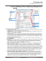
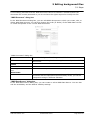
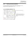
Deleating component prices and assembly times
"Delete component prices/assembly time" button
Activate the Delete Prices and Assembly Times for Embedded Libraries option if you wish to
delete all prices and assembly times and not pass them on with the linked drawing file.
AND Client Manual IV/C
© AND Solution GmbH
Page 43 of 452
2 Fundamentals
2.14 Network planning mode
2.14 Network planning mode
In Network planning mode, everything related to the network is displayed, that is,
everything with an electrical function. Cables can also be shown in civil works mode.
You need a library to be able to create a drawing. Please read how to open a library and
search for components in the Selecting Libraries for Object Selection section (Page 38).
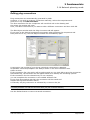
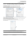
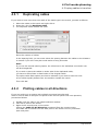
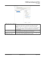
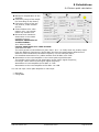
2.14.1
Plotting a component
Proceed as follows to plot a component:
1.
In the object selection window, double-click the component you wish to plot.
The mouse pointer will automatically be placed in the middle of the drawing window.
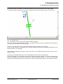
2. Move the mouse pointer to the desired position in the worksheet for the component.
The component will be attached to the mouse pointer,
which now takes the form of crosshairs because it is in positioning mode.
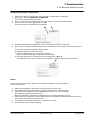
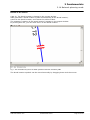
3. If you wish to rotate the component, press the R key to rotate it in 90° increments.
4. Click with the left mouse button to place the component in the worksheet.
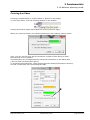
5. If automatic labeling is active, the Create Data for Drawing Object window will open.
Enter the appropriate data and click OK.
6. Now the label text will be attached to the mouse pointer.
The component related to the text is displayed red and will blink.
7. Move the mouse pointer to the desired position for the text in the worksheet.
The text is attached to the mouse pointer.
8. If you want to rotate the text, press the R key to rotate it in 90° increments.
9. If you want to resize the text, press the
2 key for larger
1 key for smaller
and 3 to 9 for predefined sizes. (For how to preview and change the preset sizes,
see the "Other Settings" section)
10. Click with the left mouse button to place the text in the worksheet.
11. If you wish to plot additional components of the same type, begin again with step 2.
12. If you do not wish to add any more components, press the Esc key to finish.
When plotting components, AND offers you a variety of supporting functions.
(See Design, Drawing, and Positioning Assistance section, Page 130).
AND Client Manual IV/C
© AND Solution GmbH
Page 44 of 452
2 Fundamentals
2.14 Network planning mode
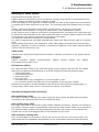
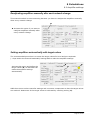
Entering the installation number and location
It is recommended that you carefully enter the installation number from the beginning of the
project because it is required for interaction with other administration programs. In addition,
these keys can be searched for across all projects when connected with the AND Smart Server.
Cables are a special case.
You should allocate meaningful cable numbers, for example,
to identify the apartment at the tap output when working with star distribution systems.
AND provides functions for automatically numbering cables
(see Automatic Numbering of Objects, Page 122).
If the Location Type is set to "current location," you can create an address in the
Location area.
If you have already created the address data for the project, the postal code,
city and street are then already preset. Also see the Project Organization section, Page 198.
It is also recommended that you allow the installation numbers to be automatically generated.
This is done based on the automatic numbering and labeling settings.
See the Automatic Object Numbering (Page 122) and
Automatic Object Labeling (Page 122) sections.
AND Client Manual IV/C
© AND Solution GmbH
Page 45 of 452
2 Fundamentals
2.14 Network planning mode
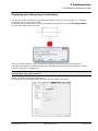
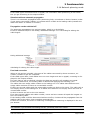
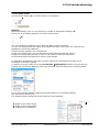
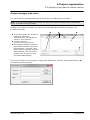
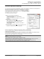
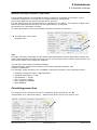
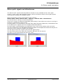
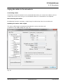
Editing plug connections
Plug connections are automatically generated by AND.
However, if you wish to create a connection manually, select the component and
press the C key for Edit Connector.
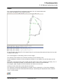
The first connection for the component will now blink red in the drawing and
the Select Pin window will open.
Here, click Next Connection if you want to edit a different connection and then click OK.
The Edit Object window with the Plug Connector tab will appear.
If you point to the desired component connection when selecting the component and
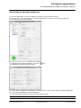
then press the C key, the Edit Object window will immediately open:
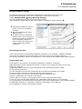
A connection can consist of up to three individual connectors or adapters.
All possible connectors/adaptors are always shown in the three Selection lists.
Select an item.
If the connection fits, the smiley will be smiling and you can click OK to save the connection.
Simultaneously, the Selection list will appear filled-in to identify the remaining options.
If the connection for the selected entry is not complete,
you can complete the connection in the middle Selection list.
If you close this window with OK, the connection will be saved and
skipped during the automatic search.
A manually set plug connection is indicated by a cross on the pin.
Note: If you move the associated icons, the saved connection will be lost. Recreate the connection list.
(The best procedure is to edit the connectors after your plan is almost finished.)
Use the Delete button to remove a saved connection.
AND Client Manual IV/C
© AND Solution GmbH
Page 46 of 452
2 Fundamentals
2.14 Network planning mode
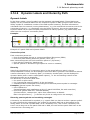
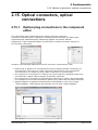
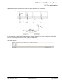
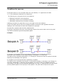
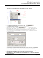
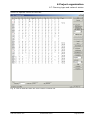
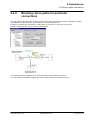
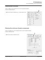
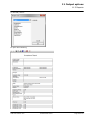
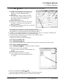
Displaying and editing the pin information
The pin information shows the type and attentuation (loss) for all connection in a network
element as they exist in the library.
To display the pin information, select the object and press the P key for Pin Information.
The Pin Information will now open.
Here you decide which pin you would like to display and edit for the selected object.
Use the Next button to switch between the individual connections that the object contains.
The active pin will be shown red.
Tip: If you select the desired connection/pin before calling this function,
that connection or pin will be shown first.
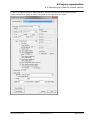
Finally, click OK to edit the selected pin.
The Connection Information tab in the Edit Ob ject window will open:
AND Client Manual IV/C
© AND Solution GmbH
Page 47 of 452
2 Fundamentals
2.14 Network planning mode
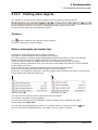
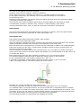
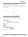
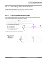
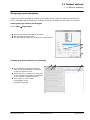
2.14.2
Plotting a cable
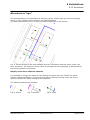
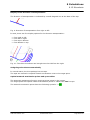
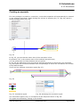
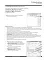
Proceed as follows to plot a cable:
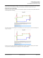
1.
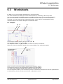
2.
In the object selection window, click the cable you would like to plot.
Move the mouse pointer to the position in the worksheet where the cable should begin.
The mouse pointer takes on the shape of crosshairs because it is now
in positioning mode.
3. Click with the left mouse button to set the cable start point.
4. Move the point pointer horinzontally or vertically to the end point.
If the cable has to be routed around a corner because of the plans,
click each of the corner points to arrive at the end point.
Press the Esc key or the right mouse button.
If the end point is on a component connection, Esc is not possible.
5. If automatic labeling is active, the Create Plotting Object Data window will open.
Enter the cable length – if it has not been automatically calculated – and click OK.
6. Now the label text for the cable is attached to the mouse pointer.
The cable to which the text is related is displayed red and blinking.
7. Move the mouse pointer to the desired position in the worksheet for the text.
The text is still attached to the mouse pointer.
8. If you want to rotate the text, press the R key to rotate the text in 90° increments.
9. If you want to resize the text, press the
the 2 key for larger
the 1 key for smaller
and 3 to 9 for predefined sizes.
10. Click with the left mouse button to place the text in the worksheet.
11. If you wish to plot additional components of the same type, begin again with step 2.
12. If you do not wish to add any more cables, press the Esc key to finish.
Plotting cables in AND is generally done by clicking individual points that will then place
the cable. A distinction is made between schematic and geo-schematic methods (see Page 27).
In schematic drawings, AND links the plotted points so that the cable only has right angles.
Please note that, in schematic drawings, there is always a preferred direction.
If, for example, you first move the mouse upward from a selected point, the cable will be
drawn such that it first goes upward, or downward, and then to the right or left.
If, for example, you first move the mouse to the right from one clicked point,
the cable will first move right, or left, and then upward or downward to the next point.
You can change the preferred direction by moving the mouse very close to the most recently
plotted point and then moving it from there in the preferred direction.
In geo-schematic drawings, you can create curves by placing very short cable lengths
close to one another.
Note: Loops are not allowed in cables and are automatically removed by AND.
AND offers a variety of supporting functions when drawing cables.
The snap function links cable ends to nearest connections (see the Snapping section, Page
132).
If you would like to make changes to a cable that has already been plotted,
for example to move it, lengthen it, remove part of it, etc.
please read the Editing and Changing Cables (Page 113) section for details of how to proceed.
AND Client Manual IV/C
© AND Solution GmbH
Page 48 of 452
2 Fundamentals
2.14 Network planning mode
Asymmetrically converted cables
Cables can be asymmetrically converted.
That is, the two ends of a cable may have differing connector references in the
component editor.
To make the location of each end of such an asymmetrically converted cable visible
in AND to the planner, it is displayed with icons that show whether each end has a connector,
a socket, and a cable, or if it is free (undefined):
Because the orientation of an asymmetrically
converted cable is relevant when searching for
the connector, you have the option
of rotating a cable.
To do this, simply choose
Rotate Cable Direction from the context
menu.
AND Client Manual IV/C
© AND Solution GmbH
Page 49 of 452
2 Fundamentals
2.14 Network planning mode
Handling of cable chains
Implemented from Build 1458 on.
Cable segments connected by sheet connectors, conduits, link objects or microducts are one
cable in reality, but different cable instances in AND.
If the edit dialog for one segment is closed with OK, the data of that segment are automatically transferred to cable segments of the chain. The following data are excepted from the transfer:
Length, cable end information, attenuation (of dark fibers), laying type, layer/color
The transfer will be applied to all types of cables (fibre, coax, twisted pair, hybrid).
In the moment when a cable is connected to a sheetconnector, the data of the outer cable will
be transferred automatically to the cables inside the sheet. It doesn’t matter whether the cable
is connected to the sheet or the sheet is connected to the cable.
The automatic transfer for blocks isn’t implemented
If a cable is created new, the cable automatically inherits the data from the cable it is connected to.
When loading old projects, the consistency of the cable chains is checked and corrected automatically ,if possible. In case of conflicts, a message is displayed in the output window and the
conflict must be resolved by user.
Cable chains
Cable pieces connected through sheet connectors, conduits, microducts or link objects build a
cable chain.
Example:
Cable1 - microduct – Cable2 – sheetconnector – Cable3 – conduit – Cable4 – link – Cable5.
All 5 cables build a cable chain.
Simultaneous editing
If a cable has been edited in the cable edit-dialog and the dialog is left with OK, the cable’s
data will be propagated automatically to all chain members except the following data:
 cable length data
 end information data
 attenuation data
 layer and color
 the cable type is only propagated, if it was changed by user
 the customer specific dot-data are only propagated, if the dot-type is equal.
Besides this exceptions all data editable in any tab of the cable dialog are propagated, i.e.
location data, defect wires, owner, individual wire owners, wire states,…
Automatic propagation after positioning
After positioning a sheet
If a sheet is moved or created, the cables inside the sheet inherit the data from the cables
connected to the sheet connectors from outside the sheet.
After creating a new cable
If a single new cable is connected to other cables viasheet connectors, conduits, microducts or
link objects, the new cable is automatically inheriting the data fromthe cable it is connected to.
The inherited cable numberis already displayedin the semi-auto-dialog. If you change the
number here it will be propagated back to all memebers of the chain.
After moving an existing cable
If an existing cable is connected to a sheet (by moving an end pin or the whole cable), the
cable’s data will be propagated automatically to the continuation segment inside the sheet.
AND Client Manual IV/C
© AND Solution GmbH
Page 50 of 452
2 Fundamentals
2.14 Network planning mode
If the cable types are different and no pigtail, the inheritation after positioning is also made,
but you get a warning in the output window.
Situations without automatic propagation
There is no automatic propagation after positioning links, microducts or blocks. Reason is that
if your action connected 2 cables, it is unclear which of both is the leading cable (transfer the
data from cable1 to cable2 or reverse?)
Propagation can be switched off
The automatic propagation is a project setting, which is on by default.
It can be switched on/off in the dialog “Additional Settings” or in the dialog for editing the
cable length:
Dialog additional settings
Subdialog for editing the cable length
Post load correction
When an old project is loaded, the types of the cables connected by sheet connector, microduct, conduit or link are compared.
If the cable types differ, both cables have non zero length and are no pigtail, a warning is displayed in the output window.
For each chain it will be checked, whether the data are equal for all members are equal.
If there are differences, the leading cable is determined applying the following rule:
The cable with non-empty cable number is the leading one. If 2 cables have different nonempty cable numbers we have an unresolvable conflict.
If there are several cables with the same cable number we look to the owner. The cable with a
non-empty owner is the leading one. If 2 cables have different non-empty owner we have an
unresolvable conflict.
As third criterion we look to the wire owners.
If we have several cables with cable number, owner and wire owners all equal the longest cable is the leading cable.
If the leading cable could be determined without conflict, it’s data will be propagated from the
leading cable to the other chain members automatically.
If there are conflicts, the chain is remaining unchanged and a warning is displayed in the output window.
Note: If you get conflicts, please be cautious when viewing the differences that you leave the cable dialogs
with CANCEL. If you would leave that dialog with OK, you already resolve the conflict.
AND Client Manual IV/C
© AND Solution GmbH
Page 51 of 452
2 Fundamentals
2.14 Network planning mode
2.14.3
Plotting other objects
The toolbar in the document window contains icons for plotting various objects.
In the following sections, you will find explanations of the various icons and
how they help to plot the corresponding objects.
Surfaces
The
button creates a new object of type "Surface."
This is a continuously closed polygon.
Marker rechtangles and marker lines
Use marker rectangles and lines to optically identify,
highlight or create relationships with parts of a drawing.
It is also possible to indicate simple topographical elements (houses, streets with houses).
Marker lines are simple line objects that have no effect on the calculation.
There are different ways to display the lines (solid, dashed, dotted, dot-and-dash).
To draw a marker rectangle or line, click the icon in the toolbar and draw it in the worksheet
in the shape you desire.
Draw a rectangle by clicking two opposing corner points in the worksheet.
Draw a line by clicking the start and end points in the worksheet.
If the line is to change the direction, click the location where the line is to have a corner point.
Finish drawing by pressing the Esc key.


Selection box ()
Selection line ()
You can also use selection lines to plot lines with free angles.
This makes it possible to draw polygons.
You can have the program automatically close a polygon line by pressing the S key,
which stands for Close Line.
You can also plot buildings and houses in civil works mode by using the building
See the Civil Works Buildings section (see Page 174) for how to proceed.
icon.
AND Client Manual IV/C
Page 52 of 452
© AND Solution GmbH
2 Fundamentals
2.14 Network planning mode
Using text objects
Use text objects if you wish to insert additional texts (, ) into the worksheet.

Use the text icon in the tools list to insert text objects:

 Text in standard font
 Text that can be formatted

We distinguish between:
 Text in the standard font
For this font you can only change the letter size, but you cannot change the font itself or
make other formatting changes.
Click the New Text
icon.
The Enter Text window will open.
Enter the desired text and click OK.
The text is now attached to the mouse pointer.
Position the text in the worksheet.
You can use the R key to rotate the text in 90° increments,
or enlarge or reduce the font size using the 1 and 2 keys, respectively.
Simply click once to release and place the text.
The Enter Text window will open again. You can enter another text if desired.
Press the Esc key to finish.
AND Client Manual IV/C
© AND Solution GmbH
Page 53 of 452
2 Fundamentals
2.14 Network planning mode
 Text that can be formatted
This type of text can be flexibly formatted.
Click the New Rich Text
icon and create a border in the worksheet
where the text is to appear.
Click in the box to open the editing window.
The Rich Text Object tab looks like a simple window in a word processing program.
Enter the desired text in the white field and format it in the same way as you would
in a word processing program like Microsoft Word.
Rich text objects cannot be rotated.
AND Client Manual IV/C
© AND Solution GmbH
Page 54 of 452
2 Fundamentals
2.14 Network planning mode
Sometimes the legibility of text is insufficient, especially when it is on a prominent background.
You can define settings for text objects to make sure the text is visible against
the background.

 Text overwrites background
 Text is transparent

Overwriting background while plotting:
Switch on the Create Text in 'Overwrite Background' Mode icon
create text with the icon
and
, as described above .
Overwriting the background subsequently:
Select the text and click with the left mouse button.
The Edit Object window will appear.
Activate the Overwrite Background option.
Overwriting the background – general setting:
Choose the OPTIONS  Program Settings  Additional Settings command.
Switch on the Create New Text in 'Overwrite Background' Mode option.
AND Client Manual IV/C
© AND Solution GmbH
Page 55 of 452
2 Fundamentals
2.14 Network planning mode
Worksheets
AND provides you with the option of using more than one worksheet at once.
The first worksheet is always the main sheet that can, if necessary, take on an NL3.
One or more headends, amplifier stations and NL4 partial networks are usually integrated
into sub-worksheets. A sub-worksheet can take on the form of any icon in the sub-sheet.
This way, you can create a clear network plan and, in the case of a topographical map,
complex stations can still be designed in schematic form.
If you wish to plot a new worksheet, use the New Sheet
icon on the toolbar.
Use the list arrow to open the list of possible worksheets and select the type of worksheet
you wish to draw.
Click the location in the drawing where you wish to plot the worksheet.
The icon for the worksheet will blink in red.
Now the description text for the new sheet is attached to the mouse pointer.
Click the location where you wish to place the text and press the Esc key if you do not wish
to plot any further sheets.
You can generate a worksheet subsequently for an already plotted component
(from the library) as follows:
Select the component and press the A key for Generate Worksheet.
The component will automatically contain worksheet connections.
The worksheet no longer represents a component, but rather the sub-worksheet.
Note: If you wish to make multiple copies of the structure of a drawing – especially in the NL4 area –
because you need the same or similar structure for other residential units, for example,
duplicate the worksheet by first saving it and loading it to the appropriate location.
Save and load worksheets with the PROJECT DATA  Project and Sheet Data command.
AND Client Manual IV/C
© AND Solution GmbH
Page 56 of 452
2 Fundamentals
2.14 Network planning mode
Sheet transitions
Sheet transitions are two-part objects for connections between worksheets.
One part is the worksheet component connection (pin, see Item ) of the worksheet icon.
The other part is the connection icon (see Item ) in the corresponding sub-worksheet.


The following types of sheet transitions are available:
 Coaxial connection (the cable type is monitored by notifications when generated)
 Optical connection (the cable type and number of fibers and bundles are monitored
by notifications when generated; in version FIBRECOAX only)
 Cable channel duct
The connection icons in the worksheet can be moved or deleted within the sheet.
They cannot be copied (especially as part of a block).
Use the P key to edit the connections.
AND Client Manual IV/C
© AND Solution GmbH
Page 57 of 452
2 Fundamentals
2.14 Network planning mode
Test points
The purpose of test points is to show the minimum and maximum level of any connections in
the drawing and can be displayed in test point list summary.
Test points each consist of 3 objects:



the test point icon (, cross or level display)
the point (, small square on the connection)
and the label ()



You plot a test point as follows:
1.
Open the list of test points on the toolbar and select the type of test point you want.
2.
Move the mouse pointer to a component connection or cable
(the point will be shown red).
Click with the left mouse button.
The test point will be placed there.
Move the mouse pointer to the location where the test point is to be placed and
click with the left mouse button.
The Create Drawing Object Data window will appear.
Enter all necessary data.
Now move the mouse pointer to the location where the label should be and
place it there by clicking the left mouse button.
Press the Esc key to finish.
3.
4.
5.
AND Client Manual IV/C
© AND Solution GmbH
Page 58 of 452
2 Fundamentals
2.14 Network planning mode
Changing connections
If you wish to change the connection on which the test point is to show the level,
you only need to move the test point to another connection.
Updating test points
If the Automatically Update Test Points option is switched on in the
Test Point Settings window, all test points in that worksheet will automatically be recalculated
when a significant change has been made to the network.
Further information about calculating connections can be found in the
Calculating Test Points section (see Page 360).
If this option is not activated, you can update all test points in the worksheet by clicking
the Update Test Point List icon ().

Labeling test points subsequently
There are two ways of labeling test points subsequently:
1. Move the mouse over the test point (test points changes color to lilac), right-click,
and choose "T Label":
2. Move the mouse onto the test point (test point changes color to lilac) and press the T key.
AND Client Manual IV/C
© AND Solution GmbH
Page 59 of 452
2 Fundamentals
2.14 Network planning mode
Showing levels
If you would like to see detailed level information for a test point,
click the test point and the following window will open:
In this window, you can enter the test values in the Measured column,
which is used to compare the actual and the target values.
You will find more information on this topic in the Calculating Test Points section
(see Page 360).
You delete a test point by deleting its test point component.
Associated objects will automatically be deleted.
AND Client Manual IV/C
© AND Solution GmbH
Page 60 of 452
2 Fundamentals
2.14 Network planning mode
Headend frame
The headend frame does not save any information.
It is meant to enclose headend components in order to use alternate calculation methods
to those for the distribution network.
However, this is normally not necessary.
If you wish to save information about the headend location,
use the location rectangle instead of a headend frame.
Draw in a headend frame using the New Headend Frame
icon on the toolbar.
Open a rectangle by dragging with the mouse.
Location rectangle
Addresses are normally the most important keys for accessing information.
AND allows you to store an address for an entire project or just for each component.
You can use the location rectangle to enclose parts of a drawing and
assign an address to the rectangle.
For example, you could define a location rectangle for a house.
Location rectangles have advantages not available with normal address entries:
 The "Object from the Management System" type sockets in a location rectangle
can store subscriber data.
 The apartment layout can be created ("Object from the Management System" type)
 Building objects and addresses are written and indexed for every location rectangle with
the corresponding label (type + no.) in the AND Smart Server database.
 The NIS schematic plan generator in AND FIBRECOAX keeps track of the individual
assembly groups within a location rectangle.
Draw in a new location with the New Location Rectangle
Open a rectangle by dragging with the mouse.
The Create Drawing Object Data window will open.
Enter the data here.
AND Client Manual IV/C
© AND Solution GmbH
icon on the toolbar.
Page 61 of 452
2 Fundamentals
2.14 Network planning mode
Using the location Rectangle for Searches
You can use location rectangles to search for objects and components.
1.
2.
Choose PROJECT DATA  Locations from the menu.
The Select Location will open:
3.
4.
Click the desired location in the list shown and then click Search.
A blinking red rectangle will now appear in the drawing.
All objects within this rectangle belong to the searched location rectangle.
Note: If you are working in an AND server environment or a GIS area environment,
the locations will also be found in unopened drawings.
Many network operators now also require that you enter the location rectangle.
You will find a detailed description of the search options in the “GIS Area” Manual (see Section 1.2).
AND Client Manual IV/C
© AND Solution GmbH
Page 62 of 452
2 Fundamentals
2.14 Network planning mode
Amplifier lists
Descriptions, levels, entry and exit points, and equipment for selected amplifiers
are displayed in amplifier lists in the drawing.
To draw in an amplifier list, use the New Amplifier List
icon on the toolbar.
Open a rectangle by dragging with the mouse.
 Inserting the amplifier in an amplifier list:
Select the amplifier and press the V key for Insert in Amplifier List.
The amplifier will blick red. Click the amplifier list in which you wish to place it.
You can also select multiple amplifiers (rock) together and place them in the list.
 Deleting an amplifier from an amplifier list:
Select the amplifier and press the U key for Delete from Amplifier List.
The amplifier will be removed from the list.
Assembly components
The purpose of assembly components is to complete the component list
with non-electronic materials.
They are assigned to the drawing objects.
Each object can possess multiple assembly components and each assembly components
can have multiple entries.
Assembly components are defined in the library using the component editor.
There are two types:
 Length objects can only refer to cables and converts;
the length of the referenced object will be seen as a quantification
of the assembly component.
 Part objects can only refer to icons.
Assembly components store the following information:
 Assembly component entries
 Reference object for quantification
AND Client Manual IV/C
© AND Solution GmbH
Page 63 of 452
2 Fundamentals
2.14 Network planning mode
Assigning assembly components
1.
2.
3.
4.
Select the object to which you wish to assign an assembly component.
Press the X key for Assembly component
The Library View window will open.
Here, you will find all objects that you can assign. Select the desired object.
You will now see a line () and a text ().
These represent the assembly component.

5.
6.

Position the assembly component near to the object to which it belongs.
If you wish to assign additional assembly components to the object, proceed as follows:
a) Click the existing assembly components.
b) The Edit Object window will open.
c) Click the Add button. In the list that appears,
select another assembly component and click OK.
d) Use this procedure to add any further components () and
click OK when you have finished. The assembly components will now be shown:

Notes
If you would like to quickly assign an assembly component to many objects,
proceed as follows:
1.
2.
3.
4.
5.
6.
Select the assembly component and press the N key to copy.
The copied assembly component is now attached to the mouse pointer.
Move the mouse pointer to the component to which you wish to assign
the assembly component and click it.
Now the assembly component is attached to the component with its line.
Move the mouse pointer to the location where the assembly component should be and
click again with the left mouse button.
To assign it to another component, repeat from step 2.
Press the Esc key to finish copying.
AND Client Manual IV/C
© AND Solution GmbH
Page 64 of 452
2 Fundamentals
2.14 Network planning mode
OLE objects
OLE objects offer the option of displaying data from any third-party programs
(OLE servers) in AND.
To insert an OLE object, choose the EDIT  Insert New OLE Object command.
The Insert Object window will open:
Select the object you want to insert from the list below Object Type,
for example Microsoft Excel Worksheet, and click OK.
Now draw a frame in the worksheet where you want to display the object.
When you click the frame, the program where you can enter the data will automatically open.
When you have finished entering the data, close the program again.
The data will now be shown in the frame.
AND Client Manual IV/C
© AND Solution GmbH
Page 65 of 452
2 Fundamentals
2.14 Network planning mode
Ruler and GIS scaling
The ruler provides scale information in the drawing and can be used to change the scale.
This is how to plot in a ruler and define the scale:
1.
2.
3.
4.
5.
Click the New GIS Scaling
icon on the toolbar.
Draw in a ruler by clicking the start point (left) and the end point (right) with the mouse.
The Create Drawing Object Data window will open.
Enter the length of the ruler.
A query window will open in which you must decide whether the scale will be activated
for the cable length calculation for this sheet. Click Yes.
Another query window will appear if the automatic component scaling is activated.
Now you must decide whether the objects should be scaled.
Click Yes and all objects will be adjusted to the size.
You can only draw in one ruler per sheet.
You can grab the ruler on the right side at any time and change its length.
The label text will be constantly updated as you do this.
Note: Use this function with caution as all existing objects will be resized and may become too large or
too small for the worksheet.
Make sure that reasonable values are entered in the worksheet dialog box for the component scaling.
See also Editing Background Files (see Page 175).
Tip: Draw in the ruler at any angle along a known length of an object.
After you have set the scale, move the ruler and press the 0 key. The ruler will now be horizontal.
Optical transmitters
Optical transmitters are the source of optical signals.
Optical transmitters have fixed output ratings (see above).
The channel modulation must be specified for each transmitter under Dynamic Data.
The program corrects the value specified for the calculation if the value is not feasible for the
current channel capacity. The channel modulation value has no effect on the output power.
If the optical receiver is unregulated, the channel modulation has an effect on the
receiver output level. The channel modulation also influences the distortion products.
In the library you can specify the connection between the input level and the channel
modulation. Using the list, the channel modulation can then be determined from the input level
and you no longer need to specify the modulation in AND.
However, this is currently not implemented in the program.
You also have the option of specifying a target reception level in AND
for the return path transmitters.
AND Client Manual IV/C
© AND Solution GmbH
Page 66 of 452
2 Fundamentals
2.14 Network planning mode
Optical receivers
Optical receivers are often also called transceivers.
There are regulated and unregulated optical receivers.
For regulated optical receivers the output rating is fixed by internal regulatory electronics as
long as the input rating is within the permissible range.
The output rating is also independent of the channel modulation.
For unregulated receivers the output level is dependent on the input rating and
the channel modulation. The dependency on the channel modulation is described
(for a particular input rating) in the library as a list of value pairs
(channel modulation | output level).
For the dependency on the input rating, a 2:1 rule is used.
An increase in the input rating of 1 dB increases the output rating by 2 dB.
For unregulated amplifiers, the output level for any input level and channel modulations
can be calculated using the list and the 2:1 rule.
Like for amplifiers, you can also define attenuation regulators for optical receiver and
slots for attenuators. Unlike amplifiers, the control options are behind the actual receivers.
Optical amplifiers
Optical amplifiers (EDFA) are treated as objects with fixed output ratings.
If the input ratios for an EDFA are not within the permissible range, a warning is output.
If "n" wavelengths exist at the input to the EDFA, the output power of the amplifier is
reduced by 10 * log10 (n).
Constant Gain Mode For Optical Amplifiers
Implemented from Build 1205 on.
In AND you can set an optical Amplifier to constant gain mode. In this mode the amplifier has
fix amplification.
Amplification and power are editable for a given amplifier in AND.
Details
If you click on an optical amplifier, you see by default the following subdialog:
In this dialog you can switch between the modes.
AND Client Manual IV/C
© AND Solution GmbH
Page 67 of 452
2 Fundamentals
2.14 Network planning mode
In constant power mode the amplifier is regulated to a fix output power. That power is the
total power of all signals together. I.e. if you have a total power of 20 dBm and 4 signals, each
signal has 14 dBm, if you have only 2 signals you have 17 dBm for each signal.
Constant power mode is the initial value after creation.
In AND 4.4 and lower all optical amplifiers were in constant power mode.
In constant gain mode the amplifier has a fix amplification. Each input signal will be amplified by that amplification.
By default power and amplification are given by the values out of library. They can be optionally overwritten by user.
AND stores, whether the values are user edited. If you do a group replacement for an amplifier
and amplification and power are not edited until now, the new amplifier will inherit the values
from the new library object. But if that values were user edited, they will be kept.
AND Client Manual IV/C
© AND Solution GmbH
Page 68 of 452
2 Fundamentals
2.14 Network planning mode
Optical terminal devices
The Edit Object window contains the Terminal Device tab for physical terminal devices
(laser/optical receivers):

 Create reports about all
terminal devices and routes
for the selected customer.
 The listed customers are
entries from the global project
customer list.
Edit the list with Add and
Delete.


Service () is an entry from the global project list of optical services,
which you can edit under CALCULATION  Edit Optical Services.
The services are also used for generating a network structure.
Terminals can now also be entered in optical input/output points
Implemented as from 4.x.869
Dialog box for entering the terminal data of an optical input/output point
The rack position and the purpose are only displayed in the optical calculation result
if the input/output point is not connected to any partner point.
In the case of connected input/output points, the data of the terminal from the partner project
are displayed.
AND Client Manual IV/C
© AND Solution GmbH
Page 69 of 452
2 Fundamentals
2.14 Network planning mode
Semiautomatic dialog box for bundles
Implemented as from Build 820
After you have drawn in or copied a bundle, the following dialog box appears
by default with the most important bundle data:
The dialog box is already filled with the default values.
So you do not need to make any entries, but only confirm with OK.
The default values for the order number and object status are defined on the
"Planning Type and Status" toolbar.
The other data connection type, fiber status, priority, and attenuation are taken
from the fiber bundle settings.
Display of the dialog box can be suppressed by clearing the "Display Editing Dialog Box"
checkbox in the settings for numbering and labeling for bundles and all planning types:
AND Client Manual IV/C
© AND Solution GmbH
Page 70 of 452
2 Fundamentals
2.14 Network planning mode
Block editing function also for bundle data
Implemented as from Build 816
The data of the semiautomatic dialog box are also offered in the block editing function:
The block in the above figure contains four bundles ( "Bundles: 4" ). Connection type, fiber
status, priority, and attenuation are entered in the "Special Properties No. 3" dialog box,
Bundles tab.
The selection boxes for setting the status and order are to be found on the "Shared Properties
No. 1" tab card.
AND Client Manual IV/C
© AND Solution GmbH
Page 71 of 452
2 Fundamentals
2.14 Network planning mode
Fiber optic cables
The special feature of optical cables is that they can contain multiple bundles of multiple fibers.
The attenuation values in the library refer to 1 km.
You can specify attenuation for various wavelengths in the Component Editor.
When drawing, AND checks both fiber type (optical/RF) and quantity.
For example, only singlefiber optical cables can be connected at the output of optical
transmitters. If the type is incorrect you will hear a beep.
You can connect optical cables - with any number of bundles and fibers to Mechanical Cable
Connection type connections.
You can also connect fiber optic cables via conduits.
Automatic Route Connection
Implemented from Build 4.5.1408 on.
If a fiber route between 2 sheets is selected, AND offers a function to create the required insheet connections automatically.
How to call the automatic creation
If a fiber path is selected in the output window, the command “Connect route automatically” is
offered in the context menu of the selected route.
The Route from Sheet A to Sheet E is selected and if you right click on the blue line, the
command for automatic connection is offered in the context menu.
What automatic connecting is doing
If the automatic connection is called, AND searches in each inner sheet (here: sheets B and C)
for already existing connections between free wires. The missing connections are created. If
there are several possibilities, existing coherent blocks and existing connections are preferred.
Each created object and each existing connection is logged by a line in the output window, i.e.:
AND Client Manual IV/C
© AND Solution GmbH
Page 72 of 452
2 Fundamentals
2.14 Network planning mode
If you click on a line “Created Object...” AND jumps to that object.
For the other lines AND is jumping to the sheet symbol.
Kind of connection defined in the project settings
For the kind of objects to be created you have the choice between links, bundles and automatic.
This is a project specific setting stored within the project.
It can be edited in the dialog appearing on the following menu command:
If Used Object Type is set to Links, the pin pairs in the sheets are connected using a pair of
link objects.
If Used Object Type is set to Bundles, the pin pairs are connected using a bundle. The attributes of the created bundles can be defined in this dialog (Connection type (Spliced/patched...),
wire state, priority).
If Automatically is set, AND will use bundles, if at least one of the 2 pins to be connected belongs to an Autosplicebox. Otherwise AND will use links.
In the combo box Object State you set state of all objects created during automatic connection.
Requirements
The sheets contain no multiplexing elements (Splitters, DWDM)
Automatic connection does not support multiplexing elements (path dividers) inside the sheets.
In this case the following warning is displayed in the output window.
Sheet <sheet name> is containing a multiplexer or splitter. Maybe the result must be corrected manually.
AND Client Manual IV/C
© AND Solution GmbH
Page 73 of 452
2 Fundamentals
2.14 Network planning mode
If you have luck the result is still OK. If not, best is to establish the connections in the splitter’s
sheet manually and afterwards calling the automatic connection function once more.
Equal wire count on both sides
If the wire count of the two pins to be connected is equal on the whole route, AND creates the
connecting links or bundles.
The blue bundle is connecting two 12-wired pins, the red and green one are connecting two
single wired pins.
If the wire count of the pins to be connected differs, AND is changing nothing in the whole
route and the conflicting pins are displayed in the output window:
AND Client Manual IV/C
© AND Solution GmbH
Page 74 of 452
2 Fundamentals
2.14 Network planning mode
The automatic connection function wanted to connect the 12-wired pin of Bundle 1 on the right
side with 2 single wired pins of Bundle 1 on the left side. The function was aborted and the
conflicting pins are displayed in the output window.
Enough usable wires
AND is never changing already existing connections in the sheets, it only creates new connections.
Existing connections lead to constraints. Wires can be free, but not usable because of two reasons:
 an existing connection is leading a free wire out of the route
 an existing connection is leading a free wire to a not free one (reserved, planned, in use,
…)
The cable from B5 to B4 has formally 46 free wires. But in Sheet B4 we have already existing
connections which lead 36 of those wires to B6. Those 36 wires are unusable for the automatic
function. (The automatic function would have to remove the existing connections in order to
AND Client Manual IV/C
© AND Solution GmbH
Page 75 of 452
2 Fundamentals
2.14 Network planning mode
use them, but modification of existing user drawn stuff is forbidden). So we have only 46-36
=10 usable wires in that cable.
Existing connections can reduce the usable wires even if they stay in the route. Imagine a
connection in a sheet which connects a free wire with a reserved wire. The formally free wire
isn’t usable, because we would automatically use the reserved wire too.
Requirement: Correct Arrangement of Autospliceboxes
Enough space between the Autospliceboxes
AND uses for each bundle a specific course, which avoids unnecessary bundle crossings. In the
following picture all 72 wires are 1:1 connected using 28 bundles:
If we would decrease the distance, we would get something like this:
In order to “look well” the distance between the boxes must be at least their height.
I.e. for the situation shown in the above picture we want to connect 28 bundles. The height of
the Autospliceboxes is 28 pin grids so we need at around 28 pin grids horizontal distance.
AND Client Manual IV/C
© AND Solution GmbH
Page 76 of 452
2 Fundamentals
2.14 Network planning mode
Such a minimum distance is also needed, if at the moment there are fewer bundles. This is
because AND reserves space for bundles which may be created later.
Swapping
In order to avoid unnecessary bundle crossings it is in most cases recommended to have one
Autosplicebox swapped and the other not.
Out of beam
If the Autospliceboxes are not face to face, a splicebox shouldn’t be in the beam of the other:
Autosplicebox B is in the beam of Autosplicebox A, the found courses have unnecessary crossings.
Both spliceboxes aren’t in the beam of the other one and so the resulting courses look fine.
Complex Sheets
In complex sheets containing cassettes or devices the course of the bundles will be rarely correct. Manual customizations will be necessary. The automatic function is still helpful, because
you can use the logged objects as proposal which you can work through.
Fibre breakage search direction can be specified
Implemented from Build 4.5.1492 on.
AND Client Manual IV/C
© AND Solution GmbH
Page 77 of 452
2 Fundamentals
2.14 Network planning mode
When searching the fiber breakage at a given distance, the search direction can be entered
too:
If we have 2 pins at the start point of the fiber breakage search, we have 2 possible directions
to start routing:
a) walking through the object the first pin is belonging to
b) running through the object of the second pin.
In the very most use cases one of both connected objects is more cable like. This is used for
specifying the direction.
If into cable is activated, the routing is started by walking through the more cable like object,
otherwise routing is started in the opposite direction.
AND is using the following list for the decision how much “cable like” an object is:
- Real cable
- Bundle
- Autosplicebox
- Logical object (Link object, Sheet connector,...)
- Real Symbol
I.e. if you connect a link with the pin of a real symbol, the link is the cable like side, because
logical objects are in the list higher than real symbols.
If you have at the start point 2 objects with same rank in the list, i.e. a cable connected to
another cable, the cable side is the side of the start object (The object which was selected
when breakage search was called).
Color codes of fibers
Fiber optic cables are themselves made up of bundles of individual optic fibers.
To be able to distinguish between these individual optic fibers,
colors are assigned to the bundles and fibers based on color codes.
Cables are assigned different codes.
Therefore several color codes can be created for cables.
Color codes can be defined in LibEdit. 256 (or 255) colors are available for this.
The color codes are stored in the library and apply to all programs.
If a conflict arises when a library is opened because the ID, name, and codes of the library and
program differ, the program asks whether the ID should be replaced or the code overwritten.
The color code assigned to a cable can be viewed in AND in the object properties
(bundle/fiber settings).
If a cable has not been assigned a color code the program uses a standard color code
that is defined in AND.
If a color code contains fewer colors for fibers or bundles than are actually contained
in the cable, the color code for the n+1 bundle/fiber starts from the beginning again
(n = max. index color code), that is, with the first color etc.
CdsClasslib/Colordef.h now contains the table “AndExtColors” for 255 colors with 255 color
values, whereas “AndColors” only has 128 entries.
CCustomColors in CdsClassLib administers these color tables.
In order to access the Ext-color table, the index is shifted to the two higher bytes and
rounded with OLIDX_FROM_SPEC_PAL 0xFF.
This tells the program to read from the Ext table.
The controls that display the colors are dynamically generated in the dialog box for color code
management. They are dependent on the number of bundles and fiber colors.
Previously, color codes only contained single-color entries without patterns.
AND Client Manual IV/C
© AND Solution GmbH
Page 78 of 452
2 Fundamentals
2.14 Network planning mode
Coloring free fibers
Coloring is implemented in version AND 4.0, Build 710 and higher.
To color free fibers, click the following button on the toolbar:
Clicking this button again deactivates the coloring function again.
When you click this button, the following dialog box with coloring options opens:
Here, you can set the color and the minimum number of free fibers to which that coloring
is to be applied.
This dialog box can be suppressed by setting a checkmark in the dialog box.
To reactivate the dialog box again, open
OPTIONS  Program Settings Thematic Colouring and
set the “Input Dialog Box” checkmark:
AND Client Manual IV/C
© AND Solution GmbH
Page 79 of 452
2 Fundamentals
2.14 Network planning mode
Dark Fiber
Dark fibers are described in AND by cables, for which the attenuation is entered by user.
Manually entered Attenuation
For every fiber or coax cable the attenuation from library can be optionally overwritten by
manually entered values.
The attenuation can be entered as list of wavelength-attenuation pairs. AND uses as
attenuation at a given wavelength the value determined by linear interpolation between the
neighbour frequencies. The number of pairs in this list is dynamic. User can insert as much
pairs he wants.
The entered values are absolute attenuations (not per km) and do not change, if the length of
the cable is changed later.
If a cable with manual attenuations is copied, the manual attenuations will be copied too.
If the cable has more than one wire, the attenuation applies to all wires.
Crosstext-labels functionality is not changed. This manual edited attenuation could not be part
of a label.
GUI
In the Edit-Dialog for cables, there is an additional tab named “Attenuation”.
In this subdialog you can set the attenuation to manual. If it is manual, a list control becomes
visible, in which the points of the wavelength-attenuation list can be inserted, edited/deleted.
Edit Value:
Left click on a value and type
Insert:
Right click into the list and select in the context menu the command Insert Row.
A new line will be added at the end of the list. After you have entered wavelength and
attenuation, you can resort the list by clicking on the header of the wavelength column
Delete:
The command Delete Row is available in the context menu or as shortcut, if at least one row is
selected. In order to select a row click on the left edge of a row (left of the wavelength
column). Multiselection using shift and control key is implemented.
AND Client Manual IV/C
© AND Solution GmbH
Page 80 of 452
2 Fundamentals
2.14 Network planning mode
Use Case
Creation of a dark fiber in library
In one of your standard libraries you create a fiber cable named “Dark Fiber”.
If you want, you can assign a special color or line style to the dark fiber, so that it can be
easily distinct from normal cables in AND.
As Order-No and Article-No you enter nothing to avoid that it is counted in the bill of material
The attenuation in library is irrelevant, because you will overwrite it in AND.
If you need dark fibers with more than one wire, you have to create extra library objects for
the various wire counts.I.e. one with one wire, one with two wires and one with four.
Using a dark fiber in AND
You insert the dark fiber as any other cable.
In the tab “”Cable data Nr.1” you switch to manual length (if you are in a Geo-Project) and
enter the length.
In the tab “Attenuation Nr.4” you switch to manual, optionally add remove wavelengths, and
enter the attenuations.
AND Client Manual IV/C
© AND Solution GmbH
Page 81 of 452
2 Fundamentals
2.14 Network planning mode
Bundle objects
Bundle objects represent the virtual connection within splices –
that is, between two auto-splice boxes.
They inserted via the 'toolbar'
.
They have the following properties:
 Connection type: spliced, open, connected …
 Attenuation: Depends on connection type; open bundles have no attenuation as no
connection exists; unspliced bundles have no attenuation because the cable is
extended without interruption.
 Costs: Individual costs entered by the user or costs that were stated in the settings.
 Length: Always 0 m.
 Graphical symbol: Depends on the connection type
 Priority: high, medium, low
 Description: Comments entered by the user
The connection type is indicated by a graphical symbol at the center of the bundle.
You can edit the graphical symbol in the bundle settings.
Bundles connect individual fibers or closed bundles.
The number of connections always corresponds to the minimum number of fibers at both ends.
Bundles that only contain individual fibers are represented by a thin line and a small symbol;
bundles that contain more than one fiber are represented by a thicker line and a large symbol.
Previously, the distance between closed bundles was always as large as an expanded bundle,
so that the large symbols could be used without any problem.
Notice: The auto-splice box can be drawn in a space-saving manner, so that bundles are only one pin grid
apart and the large splice symbols do not overlap.
Bundle objects adopt the color(s) of the fibers/bundles of both sides as far as
to the center in each case.
White bundles on the splice box are given a black border.
Bundles that would actually be white are shown light gray.
Example: Splicing between auto-splice boxes
Bundles have a material value and are included in the bill of materials (materials list).
There, a decision can be made as to whether all splice costs are summated or
listed individually. The splice costs are entered in the bundle settings.
The splice costs apply to one fiber, that is, the splicing of a bundle with twelve fibers costs
twelve times the entered price.
Bundles are located inside splices in so-called cassettes or racks, or slots.
AND Client Manual IV/C
© AND Solution GmbH
Page 82 of 452
2 Fundamentals
2.14 Network planning mode
The rack or slot applies across the bundles.
However, fibers can be located in different cassettes.
That is why there are n cassettes per bundle (n = number of fibers in a bundle).
In the Object Properties, the cassette can be entered individually for each fiber or
for all fibers at once.
Besides bundle properties, the Object Properties dialog box also provides information about
connection elements (FO cables).
This includes color codes of cables, which fibers of the FO cable are connected to which
via the bundle (number in bundle= fiber, number in cable=fiberID), fiber states,
routing information (start, end), as well as connection information (connectors)
Splice boxes
There are splice boxes that were defined as a Lib object in a library, and auto-splice boxes,
that can be automatically generated at a fiber optic cable end.
Auto-Splice box
Auto-splice boxes adopt the bundle number, fiber number,
and color code of the optic fiber cable.
They are depicted expanded like fans containing the individual bundles and fibers with bundle
labeling and fiber numbers with connection lines depicted in the color code.
Each end point has a mechanical pin. Bundles can be expanded (in fibers) and collapsed again.
Fiber pins contain one pin with 1 contact point; bundles contain as many contact points as
fibers are contained in the cable.
So, for example, a closed bundle of an auto-splice box on a 3*8 cable (3 bundles of 8 fibers
each) can be connected via a bundle object (see bundle) to a closed bundle of an OF cable 1*8
(1 bundle of 8 fibers).
Auto-splice boxes show the fiber numbers (numbers 1 to 12 in the figure below).
The numbers appear relatively large so that they remain visible on the printout.
In the expanded bundle, the bundle is labeled “B1,” “B2” etc.
f a bundle is expanded, a label appears with the bundle number on the “root side”
(“B2” in the figure below). The text is positioned at the center.
Bundles, too, can be expanded by auto-splice boxes.
This makes it possible to vary the position of the auto-splice box more, for example,
in a cassette frame. In the figure above, the green bundle “B2” is expanded into its 12 fibers.
Splice boxes can be drawn in a space-saving way, that is, the closed bundles are exactly 1 pin
grid apart. If they are not drawn in a space saving manner, the bundles are placed at the position in the object where they would lie if the bundles were expanded.
The bounding rectangle is recalculated and adapted accordingly.
AND Client Manual IV/C
© AND Solution GmbH
Page 83 of 452
2 Fundamentals
2.14 Network planning mode
For comparison: The same splice box on a 4*12 FO cable depicted in non-space-saving
manner (left) and in space-saving manner (right)
Splice boxes have output and input pins that are interconnected by so-called links.
In the case of non-automatic splice boxes, the user connects the pins manually or
with an automatic splice function in the properties dialog box (AND, LibEdit).
In auto-splice boxes, the links are automatically generated.
Splice boxes are automatically mirrored when they are drawn if the first bundle or
fiber pin is neither positioned top or right. Subsequent mirroring is also possible.
This is done by removing the pins and links and the frame with the pins are regenerated,
but exactly in the reverse order including the links.
(CreatePins, CreateLinks in CDrwObjAutoSplicebox in Netlist).
When drawing or changing the appearance of auto-splice boxes remember that the auto-splice
boxes remembers the position of the input pin as the fixed point from which the new position
of the object is determined. The position of an object is determined by the upper left corner.
Depending on the drawing setting (space saving or non space saving) and
the number of pins (number is derived from the closed bundles and fibers) and
the mirroring properties, half of the frame size is determined and
subtracted from the position of the fixed point.
The new position (top left) is then determined with RotateOffset.
If the number of pins is even, the center cannot be located directly on the pin grid,
in which case the center will be positioned on the next pin below that.
Where bundles are expanded, a handle is displayed in selection mode at the position where the
bundle would be located. If the mouse pointer is positioned over such a handle,
you can close the bundle with the ‘<’ key.
Deleting the cable also deletes the auto-splice boxes. However, any attached bundles are maintained.
 Generate an auto-splice box: Mouse pointer on FO cable end pin (selected pin) and ‘#’
key or context menu.
 Close/open bundle: Mouse pointer on grid or bundle/fiber pin ‘<’
 Drawing mode, change direction: Object properties
The object properties features a SpliceBoxCtrl which represents the connections and
the splicing (sometimes with a colored background) in the splice box.
SpleißBoxCtrl is also used in LibEdit to implement predefined splicing.
AND Client Manual IV/C
© AND Solution GmbH
Page 84 of 452
2 Fundamentals
2.14 Network planning mode
Display of the free fibers on the autosplice box
If a route is selected, the cable sections in the worksheets are also colored and the autosplice
boxes of the route indicate with an "F" the connections to which the remaining free fibers lead.
Detailed description
Fig. 1 : Route[0] has been selected in the output window and appears colored
green.
Fig. 2: Excerpt from a worksheet of the route
AND Client Manual IV/C
© AND Solution GmbH
Page 85 of 452
2 Fundamentals
2.14 Network planning mode
The worksheet connection leading to Beethovenstr. is part of the route.
The cable section has the selection color light green and the following autosplice boxes A and
B indicate free fibers with the letter 'F.'
The autosplice box A fans out in 12-core bundles. The labeling rule is "F<quantity>," e.g. "F8"
means that eight fibers are free.
The autosplice box B fans out in 1-core fibers.
The labeling rule is "F" for free and "<fiber number>" for not free.
The worksheet connection 3 is not part of the route. The incoming cable is not colored and the
splice boxes C and D do not have any free fibers.
The following figure shows the whole worksheet:
The two green cables clearly indicate from where and to where connections are needed and
the 'F' and the splice boxes clearly show which pins can be used for the new connections.
AND Client Manual IV/C
© AND Solution GmbH
Page 86 of 452
2 Fundamentals
2.14 Network planning mode
Cassette rectangle object type
A cassette rectangle is drawn around the bundle to document the position in relation
to the cassette.
Fibers and bundles automatically inherit the cassette number of the cassette rectangle
surrounding them.
The position of the splice symbol determines its association with the cassette frame.
If the splice symbol is located within a rectangle, the installation number of the
cassette appears in the splice report and on the switching plan.
The command for drawing a new cassette rectangle is listed as an item in the context menu:
The old style cassette numbers are retained in order to support cassette assignment at pure
data level, in case there is no space for the cassette frame:
AND Client Manual IV/C
© AND Solution GmbH
Page 87 of 452
2 Fundamentals
2.14 Network planning mode
The data entered in this dialog box overwrites the frame association defined by
the position in the cassette frame.
If at least one bundle with a manually edited cassette number is located inside
the cassette frame, the cassette frame provides the “Inherit cassette number”
function in the context menu:
This function deletes the data for all bundles located inside the rectangle that was
entered in the dialog box depicted above.
AND Client Manual IV/C
© AND Solution GmbH
Page 88 of 452
2 Fundamentals
2.14 Network planning mode
Automatic adaptation of cables and test points,
when auto-splice boxes are expanded and collapsed
When bundles in an auto-splice box are expanded or collapsed, connected cables and test
points are automatically adjusted to retain the connection configuration.
The two diagrams below show the example of a bundle B1 that is expanded out
in the left auto-splice box.
Before bundle ‘B1’ was expanded:
After bundle ‘B1’ was expanded:
Bundles of an auto-splice box to which cables, bundles, or test points are connected cannot be
expanded or collapsed. In such a case a message appears.
AND Client Manual IV/C
© AND Solution GmbH
Page 89 of 452
2 Fundamentals
2.14 Network planning mode
Indicating signal direction by arrows
The signal direction on single-fiber bundles and cables can be indicated by one or more arrows.
Example:
The black arrows on the fibers indicate the signal direction.
In the figure above, the yellow bundle is given one direction arrow,
the green bundle, two direction arrows.
To display direction arrows, mark a block and select the “Insert direction arrows” context menu
item. In the following figure, for example, the direction arrows are inserted for the
selected block around sheet 93:
Meaning of menu items:
 "Insert direction arrows": All single-fiber bundles and
cables are given a (an additional) direction arrow.
 "Delete direction arrows": All direction arrows in the block are deleted.
AND Client Manual IV/C
© AND Solution GmbH
Page 90 of 452
2 Fundamentals
2.14 Network planning mode
The direction of the arrows are updated manually by clicking the toolbar button
indicated in the figure below:
If there is no signal on the fiber, the direction arrows are not shown.
The arrow can be moved manually.
A red circle on the arrow tip is provided as a “handle” for this.
To move the arrow click this circle and drag it to the desired position:
Update of direction arrows is now optional
Implemented from Build 4.5.1402 on.
By default the direction arrows are updated automatically after cable editing actions.
In huge projects this can lead to performance problems, which can be solved by switching off
the automatic update.
Toolbar button for toggling
The toolbar button for updating the direction arrows has 2 states, checked and not checked. By
clicking on the button you toggle between that 2 states. If it is checked, the direction arrows of
mono fibers are updated automatically after every cable editing action (Creating a cable,
connecting a cable to a pin, moving a cable, leaving the edit dialog of a cable with OK, …). If it
is not checked, the automatic update is switched off and the direction arrows can be wrong.
Whether automatic arrow update is on or off is stored within each project.
AND Client Manual IV/C
© AND Solution GmbH
Page 91 of 452
2 Fundamentals
2.14 Network planning mode
Setting the size of splice symbols and direction arrows
You can set the size of splice symbols and direction arrows via the menu.
Do this by choosing OPTIONS Program Settings. Fibers\Bundle Settings.
You can enter the values in the dialog box that then opens:
The size of the splice symbols in AND 3.3. corresponds to a value of 200%.
AND Client Manual IV/C
© AND Solution GmbH
Page 92 of 452
2 Fundamentals
2.14 Network planning mode
The “connection information” window
All information and editing options of optical routes are listed in the
“connection information” window.
When you select and optical pin and press the ‘R’ button, the window is filled with information.
The window contains the following information columns:





















Bundle number
Bundle color
Fiber number
Fiber color
Wavelength (if a signal exists on the fiber)
Optical output at pin to which the information in the window applies
Fiber ID ("Connection-ID"). Identifier of the optical route (file type: Text)
Start address
Installation number of the start location rectangle
Target address
Installation number of the end location rectangle
Status of the route (Open/Assigned/Planned/Reserved/Splice patch order)
Priority of route (Low/Medium/High)
Intended use
Rack position of starting point
Rack position of end point
Service
User/Customer
Cable name (if the pin belongs to a real cable)
Cable owner data (if the pin belongs to a real cable)
Fiber owner data (if the pin belongs to a real cable)
AND Client Manual IV/C
© AND Solution GmbH
Page 93 of 452
2 Fundamentals
2.14 Network planning mode
This window can be docked just like the output window.
The information displayed in this window continues to be available while you are working.
You can show or hide individual columns by right-clicking on the column heading and setting
and removing the checkmark for individual columns:
You rearrange the order of columns by moving a column heading to a new position while
keeping the left mouse button pressed.
You can change the column width by dragging the heading dividing line.
Any changes you make are stored and retained when you next start the program.
AND Client Manual IV/C
© AND Solution GmbH
Page 94 of 452
2 Fundamentals
2.14 Network planning mode
The context menu in the connection information window
The context menu for this dialog box contains the following commands:
a) Context menu, edit route command
In the figure above, the route is selected through fiber 5 of bundle 6.
When you select “Edit Route,” the following dialog box opens in which you can enter
the attributes of the selected route:
The attributes Priority, Status, Fiber ID and Bundle Description are
written into all fibers of the route.
 "Only overwrite status if 'less than' ": The status of a route is only replaced
with a new status if the old status is lower in the following sequence:
Open < Planned < Reserved < Splice/Patch Ordered < Assigned
 "Only assign description to mono fiber bundles": The value of the field
“Bundle Description” is only set for single-fiber bundles.
If this checkbox is deactivated, the description is set for all bundles.
The changes made to the route are logged in the output window:
You can jump to a particular segment by clicking a log entry.
AND Client Manual IV/C
© AND Solution GmbH
Page 95 of 452
2 Fundamentals
2.14 Network planning mode
b) Context menu, color optical route command
Colors the optical route for selected fibers and lists the addresses passed through
in the output window. This function is also available for a selected pin (shortcut 'Q').
The dialog box for selecting fibers is omitted from the connection dialog box.
c) Context menu, update command
If the project from which the start pin originates is edited in a way that will affect pricing
(for example, deleting cable, changing cable length, moving auto-splice box etc.),
the editing options in the “Connection Information” window are deactivated and
the content can only be read but not changed.
With the “Update” command, the window for the start pin is filled again.
At the same time the editing options are reactivated.
d) Context menu, switch to start, switch to end command
Jumps to the end of a particular route.
This can also be done by double-clicking an entry in the “Start” or “End” column.
e) Context menu, excel-export command
Exports the window content to MS-Excel.
f) Interconnect Plan
The function has been completely revised in AND 4.0 and is implemented as from Build 777.
This function is only enabled in the FiberCoax version.
The function lists all splice boxes of a route and displays for each splice/patch cable,
bundle and fiber number from the beginning to the target.
Output has been reduced to the essentials.
The function is now called using the context menu of the Connection dialog box.
A "Print All Sheets" button has been added to the result dialog box.
Calling the function
Right-clicking a route (line) in the "Connection Information" dialog box opens the context
menu for the route:
If the "Interconnect Plan" menu item is chosen here, the following dialog box will appear with
the interconnect plan:
AND Client Manual IV/C
© AND Solution GmbH
Page 96 of 452
2 Fundamentals
2.14 Network planning mode
Interconnect Plan dialog box
One line appears for each address of the route.
If there are multiple splice/patch connections within one address, multiple lines will appear.
The first and last lines contain additionally information about the terminal.
The following five columns are shown:
Column name
Data displayed
Object
Installation number of the object of the surrounding location rectangle or the worksheet symbol For terminals (first
and last line), the rack position and purpose additionally
appears
Address
Street and house number
Connection
Type of bundle connection
From (cable, bundle, fiber)
1. End of the connection: <installation number of the cable>, B<bundle number>, A<number of cores>
To (cable, bundle, fiber)
1. End of the connection: <installation number of the cable>, B<bundle number>, A<number of cores>
If the installation number of the cable is empty, the name the cable has in the library will be
output instead.
The "Excel Export" button exports the interconnect plan to MS Excel.
The "Report" button exports the interconnect plan to the report template
"OptDurchschaltplan.rep" (German) or "OptInterconnectPlan.rep" (English).
These two templates have been modified accordingly in AND 4.0.
AND Client Manual IV/C
© AND Solution GmbH
Page 97 of 452
2 Fundamentals
2.14 Network planning mode
Example of a completed report:
The displayed name of the route ("23-11.4) in this case can be entered in the dialog box for
editing the route in the "ConnectionId" field.
The "Print Sheets" button fills the AND print preview with all worksheets of the route.
From there, the worksheets can be printed or exported in PDF format.
The "Splice/Patch Order" checkbox filters according to the "Splice/Patch in Order" status.
Bundle connections with another status are removed from the interconnect plan.
AND Client Manual IV/C
© AND Solution GmbH
Page 98 of 452
2 Fundamentals
2.14 Network planning mode
g) Locate fiber break
The distance to the break location from one cable end is entered by the user.
If the sought location is within the project, the break is labeled with a break symbol on the
cable and AND jumps to this position.
If the break location is outside the current project, the end of the route flashes and
the remaining distance to be break location appears in the output window.
AND always searches for the break from the cable pin into the cable.
The direction of the break location search is therefore already defined when the cable pin is
selected.
Starting the break location search
The search can be called in two ways:
Either directly from the context menu of one pin of a fiber-optic cable
AND Client Manual IV/C
© AND Solution GmbH
Page 99 of 452
2 Fundamentals
2.14 Network planning mode
or from the context menu of the Connection Information dialog box for the
pin previously calculated with 'R':
In a direct call, a dialog box appears for multi-core cables for selecting the fiber.
When calling from the connection information dialog box, the fiber is defined by
the selected line.
Dialog box for entering the distance
The following dialog box appears:
Here, the distance to the break location is entered.
The search direction is always "into the cable."
AND Client Manual IV/C
© AND Solution GmbH
Page 100 of 452
2 Fundamentals
2.14 Network planning mode
Result of the search
Case A): The break location is located in the current project.
AND generates a break location symbol automatically at the break location,
zooms to the break location, and causes the cable to flash.
The message "Location of the break location" appears in the output window.
By clicking this line, you can later return to the break location.
Fig. 1: The red double wavy line is the break symbol that has been inserted by AND.
The break location symbols can be moved manually by dragging them with the mouse.
AND Client Manual IV/C
© AND Solution GmbH
Page 101 of 452
2 Fundamentals
2.14 Network planning mode
The break location symbols are deleted manually using the context menu of the cable:
The break location symbols can also be inserted freely in the context menu of the cable.
Fig. 2: Handle in the center of the break location symbol
To move and activate the delete function, the mouse pointer must be located on the handle in
the center of the break location symbol.
Case A): The break location is located outside the boundaries of the project.
In the output window, a message to this effect appears, stating the remaining distance to the
break location, for example:
Fiber break is outside this project. There are 535.7 m of cable length from the last pin to the
break location.
Clicking the message takes you to the last object of the route in this project.
If the last object is a connection point with a link to a partner project, the name of the partner
project will appear as part of the output line. With the shortcut CTRL + J, you can jump to the
partner point and continue the search there with the remaining distance to the break location.
AND Client Manual IV/C
© AND Solution GmbH
Page 102 of 452
2 Fundamentals
2.14 Network planning mode
Additional properties of the “pin information” window
If you switch to another project, the editing options in the “pin information” window
are deactivated and the content can only be read but not changed.
The editing options are only reactivated when the "update" command is applied.
Caution: In wavelength multiplexing, several functions for “Set Status,” “Priority,” and “Connection ID” stop
at the multiplexer (DWDM). However, the calculation dialog box routes the signals further and displays the
real terminal units.
Setting owners of cables and fibers
The list of owners is defined by the file Owners.xml in the program directory.
The subsequent Owner Data dialog box only opens if the file Owners.xml exists:
The owner of the cable is chosen from the Owner selection box.
The cable owner is also the owner of all fibers by default.
To set alternative owners for individual fibers, press the Individual Fiber Owner button.
An additional list box with the owners of the individual fibers is now also displayed:
This list allows you to select more than one fiber (using the Ctrl and Shift keys).
An owner can be set for the selected fibers via the context menu.
AND Client Manual IV/C
© AND Solution GmbH
Page 103 of 452
2 Fundamentals
2.14 Network planning mode
Coloring free fibers
Coloring is implemented in version AND 4.0, Build 710 and higher.
To color free fibers, click the following button on the toolbar:
Clicking this button again deactivates the coloring function again.
When you click this button, the following dialog box with coloring options opens:
Here, you can set the color and the minimum number of free fibers to which
that coloring is to be applied.
This dialog box can be suppressed by setting the checkmark in the dialog box
(“Do not open this dialog box again”).
To reactivate this dialog box, open Options/Program Settings/Thematic Colouring..
and set a checkmark for Input Dialog Box ():

AND Client Manual IV/C
© AND Solution GmbH
Page 104 of 452
2 Fundamentals
2.14 Network planning mode
Function find all paths
The function is implemented in AND 4.0 as from Build 770.
The function is only enabled in the FiberCoax version.
The function lists all possible optical routes in the output windows that lead from the output
point to the target point and at least the requested number of free fibers.
The routes are output in ascending order of their total length.
Clicking on the line in the output window marks the corresponding route in color and
sets the visible section so that the entire route is visible.
Requirements
 The output point and end point must be symbols of the following type:
- optical worksheet symbol (normal case)
- optical passive component
 The output points and the fiber-optic cables must be located on the same worksheet
as a project, this is normally the GIS main worksheet of the project.
The algorithm for finding the routes treats the optical worksheet symbols as a symbol
that interconnects all the worksheet connections.
The worksheet content is completely irrelevant.
For the route search, it is immaterial whether the fibers of the route on the worksheet are
really connected from end to end or still have to be spliced.
Selection of the output point
If the symbol is a valid output point, the item "Select 1st object of the route"
will appear in the context menu of the symbol:
AND Client Manual IV/C
© AND Solution GmbH
Page 105 of 452
2 Fundamentals
2.14 Network planning mode
Options dialog
The following dialog box appears:
Here, you can set the minimum number of free fibers and the color of the routes
(project setting).
By activating the "No Longer Display this Dialog Box" checkbox,
you can suppress display of the dialog box (program setting).
The dialog options can also be changed using the menu:
Menu Options -> Program Settings -> Thematic Colouring Options...
Selection mode
After completion of the dialog with "OK," AND switches to the selection mode for the target
point. In the selection mode, the output object flashes and the mouse point is a cross.
Except for zooming and scrolling, all program functions are deactivated.
Pressing the right mouse button cancels selection mode.
Clicking with the left mouse button selects the target object.
If the target object is of the wrong type, a message to this effect will appear in the output
window and the selection mode is continued.
AND Client Manual IV/C
© AND Solution GmbH
Page 106 of 452
2 Fundamentals
2.14 Network planning mode
Output
If a correct second object is selected, the search for all routes starts and
the result will appear in the output window.
In this window, the search for the output items 3 and 8 was performed and then the line with
route[2] was clicked.
The routes appear in ascending order of their length.
The names of the stations are formed according to the following rule:
If the installation number of the (worksheet) symbol is not empty, this will be taken as the
name
Otherwise, the street and house number will be used as the name. If these are empty, too, in
the case of worksheet symbols, the worksheet name is used in a final attempt.
For lengths, spare lengths on the worksheet are taken into account.
Clicking a route colors the route with the set color.
The coloring is removed automatically if another route is selected, or if the line is deleted.
The coloring can also be deactivated manually by unpressing the depressed button labeled
"free" on the toolbar.
AND Client Manual IV/C
© AND Solution GmbH
Page 107 of 452
2 Fundamentals
2.14 Network planning mode
Selecting defective fibers
This function is implemented in AND 4.0 as from Build 788.
In the dialog box for editing a fiber-optic cable, the "Defective fibers >>" button now appears.
If you press the button, a table appears with the status of the fibers. (OK or defective).
To change the status of fibers, select the relevant fibers and
choose "Set status" from the context menu (right mouse button).
For multiple selection, you must use the CTRL and SHIFT key as usual.
Defective fibers are shown in the autosplice boxes by a large 'X':
In the figure, fibers 1 and 3 of the 2nd bundle are defective.
If the "Check network structure" option is activated for the network check,
you will receive a warning for each defective fiber to which a signal is applied.
AND Client Manual IV/C
© AND Solution GmbH
Page 108 of 452
2 Fundamentals
2.14 Network planning mode
Splice Report
The splice report can be generated for location rectangles of type ‘optical fiber point –
fibernode.’ The splice box is depicted in this location rectangle.
The edges of the location rectangle must intersect the FO cable for which the report
is to be generated.
The report determines the splicing for the cut cables and lists them.
Double entries can be ignored and the report sorted according to number of fibers
as an option.
To trigger this function, right-click the location rectangle of type “optical fiber point.”
Operating length plan
The operating length plan outputs the route between two selected points in the network.
It lists the locations, meterage data, cable type, and number of fibers.
First select a point in the network, then select a pin and in the context menu
‘Operating Length Plan’ click ‘Set 1st Position.’
If this is a pin with several contact points, you must select a contact point.
When you have done this, the route of the fiber or signal is marked.
Now you must select a second position on the marked route.
If necessary, you can abort the “Operating Length Plan” dialog box,
and then start again by setting a 1st position.
Once you have set both positions the program determines the locations that the route passes
through and stored lengths (meterage).
A warning output opens if any information is missing.
Clicking the warning indicates the object to which the warning refers.
If a splice box/splicing is passed through which has no location,
a message to that effect opens.
If the program encounters another location for which no meterage data is available,
another warning is output and the entry is skipped, if necessary.
Length information is stored in the cable pins.
It may only be stored on real cable ends, for example, not on worksheet connections.
The report is output as an “Operating Length Plan” report. Such a report can be exported or
printed out.
AND Client Manual IV/C
© AND Solution GmbH
Page 109 of 452
2 Fundamentals
2.14 Network planning mode
Coloring optical sections
It is possible to color given sections of selected optical or mechanical connections.
Select the connection and press the Q key for Colour Optical Section.
If there is a point with multiple fibers, you will be requested to select a fiber.
You will see the optical section colored in both directions from one end point to the other.
You can specify the color under
OPTIONS  Program Settings  Thematic Colouring  Signal Path Colouring.
The default color is yellow-orange.
Coloring also works for sections without signals, but for sections without signals it ends at
splitter points such as optical splitters or DWDMs.
The locations passed along the section are then listed in the output window.
When you click an entry, AND goes to the corresponding location.
This allows you to quickly find the associated terminal device.
For sections with signals, the optical attenuation between the locations is displayed.
The listed attenuations are the attenuations between the input point of the location and the
input point of the next location.
The attenuation consists of the attenuation within the location and
the attenuation to the next location.
The optical output calculation is now also possible when the transmitter contains no RF signal.
Calculating optical output for all fibers
When calculating optical output at a given point (R key) the results will appear for all fibers.
In addition to the optical output and the wavelength,
the calculation result contains a range of other information:
fiber and bundle color, fiber and bundle number, start location, end location, status,
priority and the customer for the terminal device.
It is also possible to calculate the optical output if the associated downstream laser has
no valid RF input signal.
AND Client Manual IV/C
© AND Solution GmbH
Page 110 of 452
2 Fundamentals
2.14 Network planning mode
Splice Box
Splice boces can be defined in the library or automatically generated.
If your drawing contains an optical cable that conists of more than one fiber,
you can automatically insert splice boxes on its ends.
Click a cable end and press the # key for Generate Splice Box.
AND generates a splice box, irrespective of the number of bundles in the cable and
the number of fibers in the bundle.
If, for example, your cable has 2 bundles with 5 fibers each,
the following splice box will be created:

You can always recognize the first pin in your drawing by the 1 ().
The bundles are each marked on their fibers and display the total bundle and
fiber number in brackets.
The colors of the bundles and fibers are determined in the library editor with the help
of color codes. If the fiber optic cable has not been assigned a color,
the bundle color settings of the color and bundle settings will be used.
If the auto-splice box option is selected, appropriately colored circles will light up
at the bundle locations.
At these colored locations, you can close the branched out bundles,
for example, to create one bundle with one pin and
five fibers from five individual fibers, each with one pin.
To do this, place the mouse pointer over a colored point or
an individual fiber and hold the < key or
choose the Close Bundle command from the context menu.
At the bundle location there is now a circle that is the colour of the bundle.
The digits next to the pin correspond to the number of bundles in the cable.
Branching out a closed bundle works just like closing a branched bundle.
If the entry to the splice box is not on top and not on the left,
the splice box will be automatically mirrored.
If the allocation of fibers in the automatically generated splice box in your drawing is mirror
inverted, you can mirror the pin allocation.
AND Client Manual IV/C
© AND Solution GmbH
Page 111 of 452
2 Fundamentals
2.14 Network planning mode
Click the splice box and the Edit Object window will open.
Click the Mirror Pins button.
You will find detailed information on working with optical cables in the
Optical Networks manual.
AND Client Manual IV/C
© AND Solution GmbH
Page 112 of 452
2 Fundamentals
2.14 Network planning mode
2.14.4
Editing and changing cables
You can change any plotted cable subsequently.
Moving cables
If you wish to move an entire cable, click it anywhere except the end points
(also called the "move handles") and move it.
The cursor will automatically jump to one of the two cable ends to snap it to another
connection (see the Snapping section, Page 132).
Extending cables
Select a cable end point and press the A key for Pick Up.
You are now once again in cable positioning mode, as with plotting a new cable.
You can now extend the cable as you please.
Deleting cables or cable sections
Select the cable or the section and press the Del key to delete.
The selected cable or section will blink red.
The Delete Object query window will also open.
If you wish to delete the blinking cable section, click Yes.
If you wish to delete the entire cable, click Next.
If a cable section is in the middle of the cable, the cable will be separated.
Editing cable points
What is meant here is how to change an already plotted cable.
When you select a cable, elements called handles will appear at the ends of the section
touched by the mouse.
Drag one of the handles with the mouse to change the length of the cable section.
You can also add new handles to change the path of the cable,
for example, by adding a new corner.
Hold down the Ctrl key,
drag this handle  to the desired position ,
and then release it ...
AND Client Manual IV/C
© AND Solution GmbH


Page 113 of 452
2 Fundamentals
2.14 Network planning mode
… to obtain this result:
By holding down the Ctrl key while positioning, you can add a new cable
point (handle).
Conduits
Conduits save you the effort of drawing each entire cable in AND by allowing you
to insert a cable at any location in a cable conduit and feed it out at another location.
The length of the sections between the two points occupied in the cable conduit is simply
added to the length of the two cable sections.
This way, the change in length of a cable conduit section (also called a conduit segment)
affects the length of all cables running through that segment.
In addition, conduits can also assign user cable ends automatically to cable ends that
provide signals (greatest attenuation at the highest level).
Conduits, like cables, can be easily plotted using points through
which the cable conduit will lead.
However, unlike cables, every conduit segment (every individual, straight cable
conduit section) is its own object and can be deleted, moved, copied, and selected in a block.
Overlaps and loops are not permitted with cable conduits and
AND removes conduit segments to avoid this.
There are two ways of connecting two cables through a conduit,
so that it is seen as one cable.
 Draw in two cables so that they each have an end that terminates at the cable conduit.
Select one and press the Z key for Assign.
Now the selected cable will begin to blink and AND will wait for the selection of the second
cable, which you do by clicking it.
You can also select a cable in another sheet by using the Page  or Page  key to switch.
If possible, AND will then connect the two cables.
 Draw in a complete arrangement with signal sources, splitters or multitaps,
and sockets. Route the cable from the splitters to the sockets in a conduit.
Then select a conduit segment and press the Z key for Assign.
AND automatically searches for all possible connections.
However, for it to function, the network must be error-free (calculable) all the way to the
splitter and must contain conduits because AND decides based on the splitter levels which
sockets will be connected with which splitter exit point (worst level with the shortest path).
To disconnect two cables in a cable conduit, select the cable and
press the L key for Disconnect. The two cable section will then be disconnected.
Note: Changing the length of a conduit segment automatically changes the length of the cable running
through it.
Conduits can be generated for multiple worksheets using conduit sheaths
(worksheet connections for conduits).
AND Client Manual IV/C
© AND Solution GmbH
Page 114 of 452
2 Fundamentals
2.14 Network planning mode
2.14.5
Automatic labeling of objects
After plotting an object you will be asked to position the label text.
It is recommended that you select a suitable automatic label.
Correct labeling and numbering is important for materials lists, test point lists and
other reports. See also the Automatic Numbering of Objects section (see Page 122).
Set automatic labeling with the PROJECT DATA  Numbering and Labeling command and
the Automatic Labeling tab.
AND Client Manual IV/C
© AND Solution GmbH
Page 115 of 452
2 Fundamentals
2.14 Network planning mode
In the Settings for field, you can define whether the labeling will be performed
separately according to plan types.
In the Automatic Labeling for field you can select the object type for which you would like to
set the automatic labelling.
You can define a different label type for every object type.
In the Format String field, you can define how the label will be structured.
Do this using the wildcard for the various entries in the library.
The program assists you with structuring the format string.
Click the arrow
to open the drop-down list box with all possible wildcards for each labeling
element that can be taken from the library.
You can also enter any text you wish in the format string line.
Example:
Entering “%N / %A” as the format string structure for Amplifiers will give you the following
label: 0-001-002 / 40.
The number sequence 0-001-002 is generated from the wildcard “%N”
(for the installation numbers).
The slash / was typed with a space before and after it in the Format String entry field.
The number 40 was generated by the “%A” wildcard (for amplifiers).
Activate the Update All Labels upon Exiting option to ensure that changes in the label structure
are applied in the worksheet.
If you close the Automatic Labeling and Numbering window with OK,
the settings are only applied to the active document.
If you close it with the Save Settings option, the settings will be applied to the entire program.
AND Client Manual IV/C
© AND Solution GmbH
Page 116 of 452
2 Fundamentals
2.14 Network planning mode
2.14.6
Dynamic Labels and Hierarchy Path
Dynamic Labels
In the library editor, pins of symbols can be assigned calculated labels. These labels may
display not only individual data from the respective symbol in AND (pin/port name from the
library symbol or installation number of the AND symbol instance), but also informations
calculated from the network (routing destinations), e.g. the mechanical connection end of the
connection of the pin, i.e. considering only the fibres (if known), but not the signal data.
Dynamic labels can be used to display information for library symbols (e.g patch fields) with
data from the next/final "connection point".
Example:
Example of a patch field with dynamic labels
Connection points
Final connection points are:
 Pins of terminating devices or unconnected Entry/Exit points (EEPs)
 Pins from path dividing elements (splitter, filter, etc.)
Next connection points are final connection points or (if present):
 Pins with the "Patch Pin" attribute set
 Splices (Cables or bundles of type spliced or uncut in cassette)
Hierarchy
Apart from the address of a connection point (or the start/reference point), the pin
name/installation number can be displayed. Since this data in general is not sufficient without
context information, the "hierarchy path" (or hierarchy number path) can be displayed in
dynamic labels (and is used in splice/patch reports), i.e. the surrounding context of the
pin/splice/symbol can be displayed.
The hierarchy is recursively built from
 Pin name or splice name,
 the "hierarchical parent symbols" of the pin/symbol,
 cassette/location rectangles surrounding the outermost parent symbol or rectangle.
Examples (general syntax see below):
 R0117|PF04:P01
(Rectangle/Rack with installation no.R0117, patch field PF04, Pin with name P01)
 E121:C01:[K0001.B02.F04 : F05.B06.K0002]
(Enclosure E121, cassette C01, splice from cable K0001 to K0002:
Note: the splice name [ … ] is shown only if this is configured in the settings)
Hierarchy parent symbols and containing rectangles
A hierarchy can be defined for symbols, e.g. a patch field can have a rack as a parent symbol.
In order to define this relationship, the symbol for the patch field has to be marked in the
library editor in the tab "Symbol Data" as an "Assembly Unit", and a lower "Assembly Unit
Level" has to be given to the patch field and in AND, the rack and the patch field have to be
connected via a mounting pin.
AND Client Manual IV/C
© AND Solution GmbH
Page 117 of 452
2 Fundamentals
2.14 Network planning mode
Mounting pins also may have a pin name, e.g. the mounting pin name of a symbol can be set
to "M01" in the library editor in order to name the mounting position M01. This pin name can
be displayed in the hierarchy path (if this is configured in the dynamic label settings). The pin
name of the mounting pin of the rack symbol in the library editor has more priority than the
rack position attribute of the patch field in AND.
Two documentation styles
There are thus two documentation styles (see above):
 Rack as a rectangle with installation number R0117,
containing the patch field PF04 (enter rack positionM01 in AND), Pin P01:
yields the hierarchy path: R0117|PF04/M01:P01
 Rack as symbol instance with installation number R0117,
and with patch field PF04 mounted to mounting pin M01 of the rack, Pin P01:
yields the hierarchy path: R0117|PF04/M01:P01
Hierarchy path
From the hierarchy of symbols and rectangles the hierarchy path is built as a sequence of
installation numbers (with separators) or replacements of the installation numbers:
 Parent symbols are always included,
even if they have no installation number or address
 Rectangles are included,
if an installation number or address is given
Standard syntax for hierarchy paths
 Rectangles are separated by ":"
 Mounted symbols are separated by "|"
 Pins and splices are separated by ":"
 Type and address replacement are surrounded by brackets, e.g. "(Type)"
 Rack position is separated by "/" (if appended, see settings).
The standard syntax may be changed using the "More" button of the display options dialog,
see below.
Examples:
 R0117|PF04/H4:P01
Rack-Symbol with installation no. R0117
mounted patch field with installation no. PF04 on rack position H4
pin with name pin name P01 (pin name in the library)
note: rack position H4 comes from mounting pin name of rack (library)
 R0117:PF04/H4:P01
Rack-Symbol with installation no. R0117
mounted patch field with installation no. PF04 on rack position H4
pin with name pin name P01 (pin name in the library)
note: rack position H4 comes from attribute of PF04 (no mounting information)
 E121:C01:[K0001.B02.F04 : F05.B06.K0002]
(Enclosure E121, cassette C01, splice from cable K0001 to K0002:
Note: the splice name [ … ] is shown only if this is configured in the settings)
Display / Cache
The values of the dynamic labels are cached by AND for performance reasons. Recalculation
occurs e.g. when an installation number in the project has been changed.
For regenerating all dynamic labels, you can also use the shortcut Shift+Ctrl+Alt+H (Hhierarchy): if no object is selected, then all program settings for the hierarchy paths are
reloaded and the dynamic labels are recalculated. If a pin is selected, the (physically; no signal
routing) in- and outgoing label values (%NIF, %NIN, %NON, %NOF) are displayed in the
message window (click jumps to destination pin).
AND Client Manual IV/C
© AND Solution GmbH
Page 118 of 452
2 Fundamentals
2.14 Network planning mode
Display Options for Dynamic Labels, Splice/PatchReports, Interconnect Plan, Connection
information (R function) and optical line (Q function)
Each of the functions displaying dynamic labels or hierarchy paths has a separate set of project
settings, which is accessible through the menu Project Data, sub menu Dynamic Labels / Hierarchy paths:
For the connection information (R function) there also ist the option to use the compatibility
settings.
Each of the hierarchy path settings is edited with a dialog like the following one (with a
different title and maybe some fields deactivated and with different standard values):
Hierarchy Path / Address
Hierarchy paths can be calculated for all pins of the network. For dynamic labels and
splice/patch report variables, there are even two relevant connection points:
 Start point: Pin/Splice, to which the label/report variable refers
 Destination: Pin/Slice in the net, for which data is displayed
For destinations which are not the same as the starting point, relative hierarchy paths can be
displayed to save space and enhance readability, i.e.
 if the address of start point and destination are identical, nothing or a fixed replacement
(e.g. "=") is displayed.
 the hierarchy path is displayed starting with the first differing hierarchy level of the start
point and the destination point or starting with the minimum number of levels required by
the settings, e.g.
o Start point, hierarchy path:
KS80:R018 | PF04:P07
o Destination, hierarchy path:
KS80:R018 | PF03:P07
AND Client Manual IV/C
© AND Solution GmbH
Page 119 of 452
2 Fundamentals
2.14 Network planning mode
o Display (with Min. Level < 3):
PF04:P07
For all hierarchy paths (start and destination points), the maximum number of levels can be
limited, i.e. the outer part of the hierarchy path may not be displayed, i.e.
o Max. Level:
3 (0 means no restriction)
o Hierarchy path (complete):
KS80:R018|PF03:P07
o Display:
R018|PF03:P07
The start context is the hierarchy of the start point without the lowest level (splice/pin). It is
shown in the splice/patch reports in the group line and may also occur as a dynamic label
(%CTH).
Installation Number / Pin Name
If the installation/cable number is not given, a replacement may be shown: if there is a type
and its display has been enabled, it is displayed; if there is no type or type replacement has
been disabled a fixed replacement string can be displayed. This setting is separately provided
for user defined library symbols and internal symbols. For location rectangles, the address may
also be specified as a replacement for missing installation number to be displayed. Pins do not
have an installation number. Instead, they may have a pin name supplied in the user library. If
a pin does not have a pin name, instead, the relative hierarchy path of the partner pin may be
displayed, e.g. for a sender symbol placed on a pin of a patch field, the output can be
 "Location:Sender" (without partner pin replacement, sender not mounted)
 "Location:Sender:{Rack|Patchfield:Pin}" (with partner pin replacement).
The partner pin replacement is displayed according to the settings of the respective function
(dynamic labels, splice/patch report, R function, …), only with relativization and no minimum
number of levels).
If a symbol/rectangle/pin should not be shown at all if the installation number is empty (no
replacement), just turn off replacement by type and provide an empty fixed replacement. In
this case the separators (":" or "|") are not displayed too.
Rack-Position
In addition to the installation number, the rack position or mounting pin name may be
displayed.
The rack position is determined from the attribute of the object. However, if the symbol (e.g.
patch field) is mounted and the pin name of the mounting pin of parent symbol (e.g. unit) is
present in the library, then this (mounting) rack position overrides the given attribute.
That way, in mounted hierarchies, you may work with installation number only on the topmost
mounting level (e.g. RackInst02) and the objects in between (Shelf on mounting position s1 of
the rack, Unit on mounting position u2 of the shelf, Patch field on mounting position p3 of the
unit) still have a unique hierarchy path, e.g.
RackInst02|s1|u2|p3:P01
(Assumption: the installation numbers of Shelf, Unit, Patch are empty and no replacement
option is active). This documentation style may be used to save data entry work: the name of
the mounting pin and the assembly unit level is entered once only in the Library editor.
If required, the installation number may be replaced by the rack position if it is not empty, i.e.
a non empty rack position overrides the installation number.
If the installation number is empty, it may be replaced as described above, e.g. by the library
type (in brackets), e.g.
RackInst01|(Shelf)/s1|(Unit)/u2|(Patch)/p3:Pin01
(Assumption: the installation numbers of Shelf, Unit, Patch are empty and type replacement is
active). Optionally, the type replacement can happen only if both installation number and rack
position are empty. In that case the above output again becomes:
RackInst02:s1|u2|p3:Pin01
The pin name usually is treated like an installation number (on the lowest level) and will be
displayed accordingly. For special cases (e.g. connection information, where there are two
configurable display values), the pin name can be treated as a rack position. It can then be
displayed in a "rack path" instead of a "numbers path". This only makes sense for special
documentation styles.
AND Client Manual IV/C
© AND Solution GmbH
Page 120 of 452
2 Fundamentals
2.14 Network planning mode
Splice Name
Splices are displayed using splice names, with the syntax
[<Cable No>.B<BundleNo>.F<FibreNo>: F<FibreNo>.B<Bundle No>.<Cable No>]
Optionally, the right side of the name can be displayed like the left one. Also, the prefixes for
the bundle and the fibre can be changed.
Example::
[K00001.B02.F03 : F07.B05.K00002]
(Cable No. K00001, Bundle No. 2, Fibre No. 3 to CableK00002, Bundle 5, Fibre 7)
If no cable number is given (e.g. for pigtails), the splice side may be left out altogether.
By default, the splice name is only displayed for the start point. i.e. only in reports (dynamic
labels only exist for symbols, not for splice points). The splice name display can be turned on
for destination points too, e.g. if more than one splice resides in a cassette and the cassette
information is not sufficient.
AND Client Manual IV/C
© AND Solution GmbH
Page 121 of 452
2 Fundamentals
2.14 Network planning mode
2.14.7
Automatic numbering of objects
The new numbering was created to address some issues and lack of features of the current
numbering:
 Ability to detect on object move that its counter collides with an existing one and allocating it a new one (for example when an object with a sheet counter with value 1 is moved
into another sheet where the counter 1 is already used the current numbering allocates
the object a new counter)
 Issues on sheet operations related to counters
 The new numbering allows numbering setting for a lot more object types than previously
 There exists now the possibility to have numbering settings per library object and per
metadot.
 A new counter type was added: location rectangle counter which can be used to number
all objects inside a location rectangle.
 An “external” counter type was added which allows setting of an external, global counter
(at this moment database sequence) to an object.
2.14.7.1. Setting the numbering format
LibEdit
Numbering settings can be now set for symbols and cable objects in LibEdit:
In the “Basic Data” section, the new field “Numbering format” allows one to set a numbering
format for the objects made from this library object.
Please see the section with the numbering in AND for the list of possible placeholders that can
be used here.
Metadata.xml
A new XML node <NumberingInfos> can be added to those metadots for which a specific numbering is wanted.
This is a sample node:
<NumberingInfos>
<NumberingInfo planningTypes="">
<FormatString>%P-%3S-%3c</FormatString>
</NumberingInfo>
<NumberingInfo planningTypes="Headend">
<FormatString>%3S-%3c</FormatString>
</NumberingInfo>
</NumberingInfos>
planningTypes attribute can contain one or more (comma separated) planning types for
which the current NumberingInfo applies. The possible planning types are: Headend, ALine,
BLine, CLine, DLine, ABLine, CDLine, NE1, NE2, NE3, NE4, NE5. If planningTypes is empty
than that NumberingInfo is the default numbering format.
AND Client Manual IV/C
© AND Solution GmbH
Page 122 of 452
2 Fundamentals
2.14 Network planning mode
FormatString node contains the numbering format string. Please see the section with the
numbering in AND for the list of possible placeholders that can be used here.
AND
This is the new Auto-numbering dialog:
The numbering format of an object type has now multiple sources. The numbering format is
taken if present from the next places:
1. Metadata.xml – if that object has a metadot for which numbering format (NumberingInfos
XML node from the previous section is present in the metadot definition).
2. Library object – if that object has a library object for which a numbering format is defined
(see the previous section about LibEdit).
3. Force numbering settings – this is an XML containing numbering formats for one or more
object types that has priority over the project numbering settings. Its purpose is to be
able to override current numbering settings in a project on project load.
4. Project numbering settings – the numbering settings that apply on this project.
5. Global numbering settings – this is an XML containing numbering formats for a set of default object types.
2.14.7.2. Rules of precedence
Force numbering settings and Global numbering settings are kept in the global settings path
and can be edited from AND only by users with write rights on the global settings folder.
The precedence of the numbering formats is the one from the list above, first the numbering is
searched in object’s metadot, then in its library object and so one, defaulting to the Global
numbering settings.
AND Client Manual IV/C
© AND Solution GmbH
Page 123 of 452
2 Fundamentals
2.14 Network planning mode
2.14.7.3. Editing of the numbering settings from
dialog
The elements numbered there are:
6. Planning type combo: the planning type chosen from this combo will make the numbering dialog show only the settings for the chosen type;
7. Types list: this is the list of object for which the numbering can be edited; this list is editable via buttons Add and Delete;
8. Settings source: this combo contains the list of format numbering sources mentioned in
previous section: Force numbering rules/settings, Global numbering rules/settings, Project rules/settings. The “Applicable rules” shows the numbering settings calculated based
on the rules of precedence mentioned above. Any editing made when “Applicable rules” is
selected will go to “Project rules”;
9. Format/rule edit: this edit allows one to edit the rule for the object type selected in the
list “Types list”;
10. Applies for: this multi-selection combo allows one to apply the current format to multiple
planning types. To apply the format to the planning types selected in this combo one
must press the button “11” from the image. The planning types selected in this combo
are those for which the “Add” and “Delete” buttons act;
11. Apply automatic format to: when a format/rule is changed, it is not applied automatically to the matching objects in the current project; to apply the changed format one
must choose where to apply it: “current sheet”, “current project”, “current selection
block”. The rule is applied to the planning type selected in the combo “1” from the image.
Pease notice that the automatic numbering format is applied to the objects of the selected
type and not necessarily the project or global rules/format; e.g. if an amplifier has numbering defined in its library object, that numbering format will be applied and not the project or force or global rule (this is because the library object numbering has precedence
over project of global rules – please see above Rules of precedence)
12. Create counter for objects with no counter in: this combo allows one to allocate
counter values for those objects that do not have a counter value (either the counter value is 0 per individual objects or the objects of that type did not have numbering format
before); one can choose to which objects this counter creation should apply: project,
sheet or block; also like for the “Apply automatic format” the planning type for which the
counters are created is the one selected in the combo “1” from the image;
AND Client Manual IV/C
© AND Solution GmbH
Page 124 of 452
2 Fundamentals
2.14 Network planning mode
13. Add: this button allows one to add a new object type for which numbering can be assigned. The planning types for which the new type will be created are those selected in
“applies for” combo. When the button is clicked a new dialog shows which allows one to
select one of the existing object types;
14. Delete: this button allows one to delete the numbering settings for the current object
type from the current planning types;
15. Apply: this button allows one to apply the current settings and changes without closing
the numbering dialog: the effects are equivalent to clicking OK.
16. Apply format: this button applies the current rule from “Format” edit box to the currently selected planning types (from combo “applies for”)
17. Placeholders menu: when the button with the magenta arrow is clicked a menu is presented which allows one to select from the placeholders that are replaced with values
when the installation number formatting is done. Only the placeholders that can still be
added to the format string (rule) are shown, e.g. if sheet counter (%c) is already present
in the rule it will no longer be available in the menu as project counter or location rectangle counter because only one internal (sheet counter, project counter, location rectangle
counter) counter can be present in format.
When the dialog changes are applied (by clicking Apply or closing the dialog with OK) AND
checks the validity of the formats. The things that are checked are these:
18. There can be only one internal counter (see above) and one external counter (a counter
that takes its values from external sources: currently it takes the value from database sequence) per format/rule;
19. The formats in all planning types for a given object type must have the same counters;
e.g. it is not allowed to have project counter (%C) in planning type Headend and sheet
counter (%c) in planning type NL4 for the same object; this is the same for external
counters;
20. AND checks if a counter has been changed in the format (e.g. the format changed from
having project counter to one having sheet counter in it) and performs a renumbering on
all objects of that type – this implies a setting of the new format and new numbering
(new counters are given to objects). This is done to avoid counter conflicts (clashes) between the old values and the ones created with the new numbering.
Numbering format in object properties dialog
The numbering format of an object can be seen in the object properties dialog:
AND Client Manual IV/C
© AND Solution GmbH
Page 125 of 452
2 Fundamentals
2.14 Network planning mode
For a sheet, the numbering format is present in sheet properties
and in project data dialog:
The numbering format for a project can be found in project data dialog:
AND Client Manual IV/C
© AND Solution GmbH
Page 126 of 452
2 Fundamentals
2.14 Network planning mode
Note that by default, there is no numbering format for projects. It can be defined by adding it
from autonumbering dialog (see Editing of the numbering settings from dialog).
Besides the read only dialog that shows this information, there is an 'Auto' button that allows
the user to re-set the numbering format based on the current rules and the current object
properties.
2.14.7.4. Counters in editing
If an object type has numbering format with a counter in it the objects of that type get an automatic counter value which is a free value (not used by other objects of the same type). The
user may, though, edit the counters using the context menu
When this menu action is clicked a dialog is presented where one can edit a new counter value
The current value is shown in the dialog. One can edit this value directly or use the two buttons:
Delete means that this object does not have a counter value set and the installation number
can be edited (as opposed to a read-only installation number when the counter value is nonzero). This is useful when one wants an object “outside” numbering.
Auto button searches for a free counter and allocates one to the object.
When this dialog is closed with OK AND validates the counter set in the dialog (checks to see if
the value is already used). If the value is already used a new dialog shows which gives the
user a few options to fix the counter conflict:
AND Client Manual IV/C
© AND Solution GmbH
Page 127 of 452
2 Fundamentals
2.14 Network planning mode
2.14.7.5. External counters
External counters are now available in AND in order to ensure system wide unique values. The
formatter for the external counters is %Q followed by the counter name enclose in square
brackets. Current implementation of the external counter is based on database sequences and
they can be defined from DBAdmin. There is a new TAB named "Numbering Sequences" where
a new sequence can be defined.
After defining it with DBAdmin, this is automatically available in the "Placeholder Menu" (button "12" in the figure on page 124).
The value of an external counter is resolved during the checkin of the project. Any label based
on an external counter will be formatted like %Q[<externalcounter name> : <AND Object
Handle>] and during the first check-in of the project, this is substituted with the actual value
of the external counter.
It is not allowed to combine two external counters in the same time for a particular object, it is
however allowed to combine one external counter and one internal counter (project based
counters).
AND Client Manual IV/C
© AND Solution GmbH
Page 128 of 452
2 Fundamentals
2.14 Network planning mode
2.14.8
Immediate editing of objects when plotting
It is advisable to enter object data immediately after plotting an object
(see figure below, Item ).
This is done by switching on the Display Ediging Dialog option with the
PROJECT DATA  Numbering and Labeling command and the Automatic Labeling tab.
Make sure that you make the settings for each object type () separately.


With this setting, the Create Drawing Object Data window will automatically open after plotting
an object so that you can enter the data.
If Auto is highlighted, that means an automatic length, label, or number is already set and
that this value will automatically be generated.
If you wish to enter individual values, do so in the entry field.
When you are entering individual values, the Auto button (see figure below, Item )
will be switched off:

Note: If you wish to change properties subsequently, such as the length of a cable,
always do so in the Edit Object Window (see Page 16) and not directly in the label text because
this has no effect on the calculation functions. (The label text will be adjusted automaticall)
AND Client Manual IV/C
© AND Solution GmbH
Page 129 of 452
2 Fundamentals
2.14 Network planning mode
2.14.9
Design, drawing, and positioning assistance
AND assists you in a variety of ways so that you can create
a correct network plan quickly and easily.
Rotating while positioning
AND provides the following key commands with which you can rotate an object while
positioning it:
D key = rotate through 2°
S key = rotate through 1°
R key = rotate through 90°
0 key = reset to 0°
A key = rotates to adapt to the object being positioned.
AND Client Manual IV/C
© AND Solution GmbH
Page 130 of 452
2 Fundamentals
2.14 Network planning mode
Vectorizing background plans
A background plan (see Chapter 5) can be a site plan, a topographical map,
or a story-floor plan of a building.
These plans often contain information that you do not require in your network plans.
If you do not have graphics software like AutoCAD to create plans in the necessary form,
use the AND design and plotting assistants to trace, that is, vectorize the site plan.
Proceed as follows to vectorized the site plan:
1.
2.
3.
Load the drawing you wish to vectorize in the background.
Do this using the FILE  Background  Load Bitmap Background command if you
are dealing with a bitmap graphic or FILE  Background  Load DXF Background
if you are dealing with a file in dxf format.
The graphic is visible but cannot be edited because you are automatically
in Network Plan Drawing Mode (see Page 44).
Using the Marker Rectangles and Marker Lines (see Page 52) to trace the parts of the
graphic that you need.
To make drawing and design easier, a number of snap functions are available to you.
Activate these as follows:
 Before drawing:
Click the corresponding icon on the toolbar for design assistance.
 While drawing (in positioning mode):
Press the corresponding Function key,
for example, F1.
      







Snap to end point – F1
Snap to middle – F2
Snap to intersection point – F3
Snap to joining point – F4
Snap to nearest point – F5
Activate orthogonal mode – F8
Snap to background – F11
Note: After you have traced (vectorized) a drawing, it is best to delete the background graphic to save
storage space. To do this, switch to the Arrange Background drawing mode.
Select the graphic by clicking it and then press the Del key.
AND Client Manual IV/C
© AND Solution GmbH
Page 131 of 452
2 Fundamentals
2.14 Network planning mode
Snapping
The snap function for component connections is a positioning assistant with which
you can precisely place component icons on existing icons or a cable.
That is, a component is placed such that at least one of the connections for that component
is lying exactly on an existing component connection or cable.
The snap function is automatically active and causes a component being positioned always to
be "pulled" to a connection as soon as one of the component connections approaches
an existing connection.
This happens when the distance between the two connections is less than 5 pixels.
If the mouse moves away again, the icon "disconnects" and moves with the mouse again.
As soon as a component being positioned touches a cable with the mouse cursor,
the icon on the cable will be aligned
(important: this only applies to cables on the mouse cursor, not to all cables near the
connections, because AND would otherwise not be able to decide which cable to use).
If you wish to plot a cable and attach it to a component connection, but no other cable is
connected there, the snap function is effective.
That is, positioning the cable is finished at this connection and other cable data may be
queried, that is, you can go ahead and plot the next cable.
Otherwise the cable cannot be positioned on the selected connection.
You can also receive assistance by activating the Snap with Tone option in the default settings.
A successful connection will activate a short beep and an unsuccessful connection will activate
a longer beep from AND.
If you temporarily wish to work without the snap function, hold down the SHIFT key while
positioning a component or cable.
You can make the snap function default settings (see figure below, Items  and )
with the OPTIONS  Program Settings  Additional Settings command:


AND Client Manual IV/C
© AND Solution GmbH
Page 132 of 452
2 Fundamentals
2.14 Network planning mode
Snapping components to cables
If you wish to snap a component to an already plotted cable and automatically
have it disconnected from the insertion point and connected to the component connection,
proceed as follows:
1.
2.
3.
4.
Select the component.
When positioning the component, press the F key for Snap Object.
Now drag the icon directly to the cable and it will be automatically linked.
A window will open in which you can enter the length of the cable. Click OK.
Disconnecting components from cables
The "Disconnect from Cable" function is the opposite of "Snap to Cable."
You use it to remove components from cables and simultaneously reconnect the cable.
This function is only available if a component is selected that has two opposing connections on
the margins with cables attached to the connections at the same angle and
the opposing connections have differing directions, that is, entry and exit.
To disconnect a cable from a component, proceed as follows:
1.
2.
3.
Select the component and press the H key for Disconnect.
The component is now attached to the mouse pointer.
Position it at the desired location in the worksheet.
Blocks
Blocks are an easy way to speed up work with networks.
A block is a way to select several objects at once.
A block can be given a name and saved so it can be called up later under that name and
inserted in another drawing.
You will find a description of the block copying function in the “GIS Area” Manual (see Section 1.2).
This helps you to complete your network plan more quickly, for example,
if you need to create multiple identical subscriber connections in an NL4 plan.
Read the Block Selection section (see Page 33) for how to define a block.
Uses for working with blocks include:
 You have duplicated a cable but forgotten to enter the length.
Select all the identical cables and open the Edit Object window by clicking the block.
Then enter the cable lengths on the Special Properties tab.
 A plan contains a large number of stock cables that now need to be replaced
by a new cable type.
Select the stock cable and replace it with the new cable.
 Cables are subject to different temperature fluctuations, for example,
overhead lines or buried cables.
Here, you can define temperature groups (in FIBRECOAX only).
(You will find more information in the Temperature Drift section (see Page 317).)
AND Client Manual IV/C
© AND Solution GmbH
Page 133 of 452
2 Fundamentals
2.14 Network planning mode
Saving blocks
Proceed as follows to save a block:
1.
2.
3.
Select the objects that belong to the block.
Press the S key for Save.
Enter the file name for the block in the Save As window and select a suitable folder.
Inserting blocks
Proceed as follows to insert a block into the drawing:
1.
2.
3.
4.
5.
Press the K key for Load Block in the AND drawing.
The Open window will open. Select a folder where the block is saved.
Double-click the block file name.
The block is now attached to the mouse pointer.
Position the block and click with the left mouse button.
AND Client Manual IV/C
© AND Solution GmbH
Page 134 of 452
2 Fundamentals
2.14 Network planning mode
Changing the apartment numbering in blocks
AND allows you to quickly and automatically allocated new installation numbers for all
outlets and cables contained in a selected block.
Select a block and open the context menu.
Choose the Change Numbers function and the following window will open:
If you require a standardized prefix for all generated numbers, enter this prefix in the
Object Number field (normally the object number of the building).
If you wish to define additional settings, select the Number Residential Location option.
Otherwise, all the remaining options will be deactivated and all cable and
outlet numbers will precede the numbers entered under Object Number.
If you select an option under Ascending Numbers for Floors or under
Ascending Numbers for Apartments on Floor,
you can specify that each socket and each cable is given an ascending number in the
selected direction. The starting values for floors will also be allocated.
If you select the Do Not Number Subsequent Connections option, only end sockets will be
numbered. Otherwise all (even loop-through) sockets will be numbered.
If you select the Delete Other Cable Numbers option, the cable numbers will be deleted for all
cables that are not connected to sockets whose numbers were changed.
Note: The following general standard is recommended:
Cables should contain an object number + apartment location; outlets should only contain the
apartment location. This way, the cables on the multitap can also be distinguished when the cables
converge from more than one house to one point.
To find the outlets that only have the apartment location, we recommend they be enclosed in a
location rectangle with the object number as well as the installation number.
AND Client Manual IV/C
© AND Solution GmbH
Page 135 of 452
2 Fundamentals
2.14 Network planning mode
Creating and changing amplifier lists with blocks
AND offers you the option of inserting multiple amplifiers into an already plotted amplifier list.
Select all amplifiers and create a block. These amplifiers can be in different worksheets.
Press the V key for Add Amplifiers to Amplifier List to add them.
All amplifiers in that block will be displayed in the amplifier list.
If you wish to delete some amplifiers from an amplifier list, select those amplifiers.
This creates a block.
Press the U key for Remove Amplifiers from Amplifier List to delete them.
All amplifiers in that block will then be removed from the amplifier list
(see also the Amplifier List section, Page 63).
Counting residential units in blocks
AND allows you to count the number of residential units using a block, that is,
to make collective changes for these residential units.
Select a block and open the context menu.
Choose the Count user Sockets/MDUs option.
The following window will open:
All residential units within the block will be identified, including possible sub-worksheets.
The Change Residential Units option allows you to accept changed specifications for signal
transmission points. These are important for the return path setup calculation,
among other things (because a signal transmission point represents a missing NL4 plan
at this location).
AND Client Manual IV/C
© AND Solution GmbH
Page 136 of 452
2 Fundamentals
2.14 Network planning mode
Generating bills of materials for blocks
If you need a bill of materials (materials list) for a partial section in a larger plan,
select a block over the partial section and open the context menu.
Choose the Generate Materials function.
The Edit Materials List window will open:
You will find detailed information about handling bills of materials in the Bills
of Materials section (see Page 411).
AND Client Manual IV/C
© AND Solution GmbH
Page 137 of 452
2 Fundamentals
2.14 Network planning mode
Editing objects in blocks
You can change objects in a block in one step. For example, you can change layer affiliation
and color for all objects contained in a block at the same time.
Select a block and click it.
The Edit Object window will open:
Frames
In AND, frames allow you to select an icon from a variety of display formats.
Use this function if, for example, you want to identify graphically the signal direction or
a diplex filter.
The different frames for an icon do not have to be the same size, that is,
have the same number of pins (which makes any later changes more difficult).
Frames are created in the Component Editor.
While positioning, you can switch between the various frames by using either the
Previous Frame or Next Frame functions or the 1 key (previous) or the 2 key (next).
AND Client Manual IV/C
© AND Solution GmbH
Page 138 of 452
2 Fundamentals
2.14 Network planning mode
Assembly objects / Macros
Assembly objects (also referred to as "macros" in AND) simplify the creation of complex
components out of individual parts.
A macro can consist of a maximum of 4 individual components.
Components can be assembled if they have assembly points
(see the “Component Editor” Manual).
This option is designed to simplify the combination of various equipment versions,
for example entry and exit splitters in complex amplifiers.
Another application is the mechanical connection between SAT-LNC and the parabolic dish.
AND needs this connection to calculate noise and levels from SAT signals.
This is how to create an assembly object:
1.
2.
3.
4.
5.
6.
7.
8.
Draw an object that is suitable for assembly into the worksheet.
Select the object and press the M key for Assemble Object.
The Select Assembly Object window will open:
Here, all objects will appear that can be assembled – and interchanged.
Only objects that are suitable for assembly will appear in this window.
Select an object from the list and confirm with OK.
The two objects are now connected to each other and will be treated as a single object.
If you wish to mount further objects to this, select the assembly object and
confirm with the M key once again.
The Select Pin window will now open.
You can switch back and forth between the still unoccupied pints by clicking “Next.”
The corresponding pin will be shown red in the drawing.
Select the desired pin and click OK.
The Select Assembly Object window will open again.
AND Client Manual IV/C
© AND Solution GmbH
Page 139 of 452
2 Fundamentals
2.14 Network planning mode
Planning status
If you would like to differentiate in your plan between the parts that are still being planned and
the network sections that are already completed, use the planning status.
1.
2.
3.
4.
Select the power supplies that you want to identify as being planned.
A block will be created.
Click the block with the left mouse button.
The Edit Window will open.
Under General Properties on the Common Properties tab, choose the ‘in planning’
(being planned) option from the drop-down list box for the Status.
If you select individual objects and assign planning status, you can find the status
on the Location/Installation No. tab in the Status drop-down list box.
Color settings for the various planning statuses can be defined using the
OPTIONS  Program Settings  Thematic Coloring option.
Define the status color here.
Making the planning status visible
You can make the planning status of individual objects visible by activating the
Show Planning Status in Color
icon on the Warnings toolbar.
AND Client Manual IV/C
© AND Solution GmbH
Page 140 of 452
2 Fundamentals
2.15 Optical connectors, optical connections
2.15 Optical connectors, optical
connections
2.15.1
Optical plug connections in the component
editor
The connection type is described as an optical connector reference.
Connector references can be assigned to component connections and cable ends.
Asymmetrically assembled patch cables and pigtails can also be defined.
Assignment in the Component Editor is performed in exactly the same way as for
RF connector references.
However, the following differences from RF connector references do exist:
 References of optical icon connections are either sockets (female connectors) or
connectorless. There are no "male" connector references for icon connections.
The references of a cable are either male connectors or connectorless.
 If an optical icon connection is a socket, this means that the component has to be
connected by a patch cable or pigtail of the same reference.
 If an optical icon connection is connectorless (reference to cable), this means that
the component has to be connected by splicing to a cable with the same reference.
 Optical adapters as separate components are described by icon icons of type
"optical adapter." Patch panels are typically icons of type "optical adapter."
AND Client Manual IV/C
© AND Solution GmbH
Page 141 of 452
2 Fundamentals
2.15 Optical connectors, optical connections
2.15.2
Testing optical plug connections in AND
The optical connections are tested as part of the Find Connector function,
which is called on two occastions:
 As separate function (Calculation menu, Test Optical Connections menu item, ALT+O).
 As part of the network check,
if the Test Plug Connections option is activated in the warning settings (Alt+W).
No adapter search is performed in the case of optical connections.
The existing optical connections are tested only and a warning is shown in the output window
for each unsuitable connection.
To remedy an error, you must replace the patch cable/pigtail with the unsuitable end
by a suitable item.
In the case of bundle objects, the connection is only tested if the bundle status is spliced.
A warning is displayed for this bundle if one of the two cables connecting the bundle is fitted
with a connector or the cables have different cable references.
AND Client Manual IV/C
© AND Solution GmbH
Page 142 of 452
2 Fundamentals
2.15 Optical connectors, optical connections
2.15.3
Attenuation of the optical connections
Attenuation of the plug connections
All connector attenuations are described by values of icons in AND.
AND assumes that the attentuation of the plug connections is already contained in icon values
such as attenuation / output power.
Examples:
Transmitter:
If the output power of a laser is 6.0 dBm according to the library,
AND assumes that the output power is 6.0 dBm including the connector attenuation.
The same applies to passive components.
For example, the library attentuation value of a splitter fitted with a connector describes
the entire attenuation: pure splitter attenuation + entry and exit connector attenuation.
Receiver:
AND takes the power before the connector to be the input power This is the power that you
would measure if you disconnected the patch cable from the receiver and routed the signal to
a photodiode instead.
Consequently, pure connection elements such as patch cables are also described as icons.
The icon type is Optical Adapter.
Each optical standard package of an optical adapter describes the attentuation of a connection.
Attentuation of splice points
In the calculation of the optical power, a fixed splice attenuation is assigned to each point at
which a connection without a connector is conneced to a cable end without a connector.
You can edit the value of the fixed splice attenuation in the calculation settings.
AND Client Manual IV/C
© AND Solution GmbH
Page 143 of 452
2 Fundamentals
2.15 Optical connectors, optical connections
Attenuation of bundles
The bundle objects between two auto splice boxes are abstract representations of
optical connections and are therefore a special case.
If the bundles status is plugged or spliced, the attentuation will be directly entered in the
bundle. A bundle with cut status interrupts the signal flow (without warning!),
a bundle with uncut status has an attenuation of 0.0 dB.
AND Client Manual IV/C
© AND Solution GmbH
Page 144 of 452
2 Fundamentals
2.16 Creating a new document
2.16 Creating a new document
In general, when creating a new document, we recommend the following prepared steps so
that you can use the AND automatic functions and quickly complete a correct network plan:
1.
2.
Create a new document with the FILE  New Network Plan (NET) command.
Load the libraries that you need:
a) Open the context menu in the objectt selection window,
select the Edit Libraries List command and click the Load… button.
b) The cursor is in the Quick Search entry field.
Enter the name of the library you need, for example, "neut3."
Now all items will automatically be selected that begin with the text you entered.
c) Click the Load button and then OK to load the selected libraries.
The objects will be displayed in the object selection window.
d) You can display the objects of a certain library by opening the context menu
in the object selection window and choose the Select Library command.
Use the “Neut3vrt.lib” library, for example.
2.
3.
4.
5.
6.
Enter project data:
Make a habit of recording project data for every document.
Important data includes, for example, the project number and the address
of the headend or power insertion point.
This information enables you to see which document it is and search for it
(see also the “GIS Area” Manual).
Choose the PROJECT DATA  Project and Sheet Data command.
The data entered will appear in the legend and in the reports
(see also the Project Organization section, Page 198).
Import a topographical map into the background:
If you want to create a plan that shows the correct positional arrangement based on
a topographical map, import a raster or vector map.
Choose the FILE  Background  Load Bitmap Background command or
Load DXF Background (see also the Editing Background Files section, Page 175).
Set the scale:
If the scale is not set automatically after loading the background,
draw in a ruler and set the scale (see the Ruler and GIS Scaling section (see Page 175).
Set automatic labeling
You can set defaults for labeling objects in drawings so that information,
such as type, length, unit, etc. is inserted automatically.
This simplifies your work and ensures consistent labeling.
For a detailed procedure, read Automatic Labeling of Objects (see Page 115) and
Automatic Numbering of Objects (see Page 122).
Create a layer
Layers are placed one on top of the other in your worksheet.
Choose the PROJECT DATA  Layer Table command.
In the layer list on the left, click Standard, click the New button and enter the layer name
and color. (See the Layer section, Page 216).
AND Client Manual IV/C
© AND Solution GmbH
Page 145 of 452
2 Fundamentals
2.16 Creating a new document
General procedures for creating a network plan
Creating a complete network plan involves many separate steps.
Sticking to to a specific sequence throughout will speed up the whole process.
1.
First decide whether you want to work in a schematic or geo-schematic format.
The geo-schematic method has the advantage that, in addition to network information,
it contains approximate location documentation within the plan.
Furthermore, cable lengths are automatically derived from the scale –
which speeds up your work.
The disadvantage of this method is that you have a less clear overview
of the switching plan when working in more complex networks.
This disadvantage is, however, compensated for by the NIS schematics generator
(in FIBRECOAX only).
In the geo-schematic format you have to provide a topographical map or
a site plan in DXF vector, BMP, TIFF or JPEG file formats.
Vector maps have the benefit of being zoom-independent with regard to resolution.
In many cases, such maps have different layers (levels) that are individually colored and
can be hidden.
Raster maps are typically more inexpensive and easier to obtain (for example,
by scanning). If at a later date a different trench dimensioning is needed,
raster maps will be too inaccurate.
2.
3.
4.
Load the map as a background.
The scale can be carried over when using DXF maps.
With raster maps the scale may be automatically generated from an existing ASCII
coordinate file in a GIS system format, or it must be manually entered by drawing
in a scale ruler and specifying its length.
Next, you select the necessary libraries.
These are then displayed in the object selection window.
The libraries contain all component information for items such as cables, amplifiers,
splitters, connectors, etc.
The object selection window can be configured such that only frequently used
components are visible.
Enter the project data. This is essential for clear documentation and
you can use the data to perform searches at a later date.
Now draw your network plan.
To do this, simply drag the components from the object selection window
into the drawing sheet.
If you place a tap on a cable it will rotate automatically and disconnects the cable.
If you position a cable or another component near a component connection while
positioning mode (see Page 25) is active, the nearest connection will be drawn
to it like a magnet.
In AND this is called ‘snapping.’
This simplifies your work and ensures that a correct network list can be created.
The network list assists with the calculation and requires traceable connections between
the components.
AND Client Manual IV/C
© AND Solution GmbH
Page 146 of 452
2 Fundamentals
2.16 Creating a new document
5.
6.
7.
The overview of a network plan, particularly a geo-schematic network plan,
is improved if more complex objects like amplifier stations or NL4 networks
are displayed separately in NL3 plans.
Worksheets assist you in this and you can draw them into NL3 plans like components.
Worksheets can take the form of any icons.
Open the worksheet and schematically plot the network of complex objects.
Use worksheet connections to connect this partial network with the parent network.
This ensures proper calculation.
This structure makes it possible to display headends, fiber optic networks,
coaxial networks, all node and amplifier stations as well as the network level 4
in the houses in one document (project) and retain a clear overview.
An extensive network can also be spread over multiple documents and
interlinked using "entry and exit points."
Execute the necessary level, distortion product and remote powering voltage calculations.
For this, give the signal source any frequency and level plan you wish and
give the amplifiers target values.
Do this by simply clicking the drawn objects.
In the window that opens you can enter the desired data and change it at any time.
The changes in the network can be tracked in the drawing using elements called
"live test points."
You can also select any component connection and calculate the level or
the distortion ratio.
These calculations can be done at any time during the drawing process, even if the network is not yet completed.
In addition to the calculation methods mentioned above, there is also a network check.
In the warning settings you can define exactly how your network should perform and
then use the network check button to examine everything at once.
The network check can carry out the following tests:
network structure, amplifier settings, level situation at connection points and sockets,
performance (CTB, CSO, C/N, MER, BER), remote powering, return path level,
return path C/N and return path ingress, temperature drift and plug connections.
The network check makes it easy to screen for changes in the network quickly, that is,
to see whether any drawbacks have resulted from changes in other parts of the network.
This allows you to constantly optimize the network using a sort of
"trial and error" method.
You can even use the performance calculations to track down weak links in the network
plan: the location with the weakest CTB, CSO and C/N are always shown.
By changing the system level of the affected lines, you can then further optimize
the network.
8.
9.
All warnings that occur during the calculations are displayed in the output window.
Clicking an entry causes the locations in the network to blink.
You then know exactly where to make corrections to restore network functionality.
Once you have created the network to your liking, you can print out the test point list,
the bill of materials, the drawing, or any other reports.
A variety of standard reports will be provided such as the proposal, order, performance
catalog and the acceptance protocol. Use the report designer to create individual reports.
To use test point or materials data in other programs, there is an export option for Excel.
To send reports via letter or fax use the export to Word or bitmap function.
AND Client Manual IV/C
© AND Solution GmbH
Page 147 of 452
3 Automatic drawing modee
3.1 Selecting a network type
3
Automatic drawing mode
Using this automatic function, it is possible to have AND independently create nearly an entire
NL4 broadband CATV system, or portions of such a system.
The goal was to make the function as flexible as possible but to make it as simple
as possible to operate.
Only the most essential specifications must be made;
everything else is performed for you by AND.
This function really does make your work easier when developing systems.
Start the automatic function by selecting OPTIONS  NE4 Automatic.
The Automatic Network Generation window will open.
Here, you select the type of network, define the structure of the buildings,
splitter levels and the components to be used, and determine levels at the connection point.
3.1
Selecting a network type
When you call the automatic function or click the Network Type tab in an already open
Automatic Network Generation dialog box, the following image will appear:

 Select the network type
(the “IF Matrix” option is
not avilable at this time).
 Select the type of signal source
to be be used.
 Enter the work area for which
the drawing is being created.


AND Client Manual IV/C
© AND Solution GmbH
Page 148 of 452
3 Automatic drawing modee
3.1 Selecting a network type
Entering the signal source
You can select the Connection Point signal source in the first worksheet of the project.
The component you define in the Components tab for the "Source"
parent level option will be used.
You must use the Worksheet Entry signal source for sub-worksheets.
You can only use the Headend Worksheet signal source in the first worksheet.
This cannot contain any further sheets.
The signal source is then loaded as a new sheet from the specified drawing.
Please note that the selected file must be a saved headend sheet, that is,
a sheet without entries, and can only have one exit.
Use the Change button to search for the file.
Defining the work area
Here you define whether the automatically generated network will completely fill the active
worksheet or whether it will be inserted into the active worksheet as a block.
If you selected the Worksheet work area, the network will be placed above
the active worksheet.
If the active worksheet is not empty, a question will appear asking you whether the
entire active worksheet should be used to draw the system.
The existing drawing on the sheet will be deleted.
Caution:
If you answer the question with Yes, the previous contents of the active worksheet will be deleted and
irretrievably lost! If the worksheet is too small you will be asked whether it should be enlarged.
If the connection point is selected as the signal source and the active sheet already contains signal sources,
you will be asked whether to delete these or keep them.
If you wish to reuse an existing signal source and multiple signal sources exist,
a dialog box will open after this question in which you select the signal source to be used.
Note:
If you wish to plot your system in a worksheet other than the one with number 1, and there is an entry point
in this worksheet, the default levels will be transferred to the signal source and the values calculated at the
entry point will be taken into consideration for this location.
The signal source icon will of course not be plotted.
If you select the Block work area, the network will be inserted into the active worksheet
as a block. To do this, open a block frame by dragging with the mouse.
Caution:
The system will be drawn directly into the area you specified and
cannot be subsequently moved as an independent unit.
Therefore, please make sure that you do not define the block area such that existing objects are included!
Note:
Only the distribution network without amplifiers and signal sources will be constructed with the target
area block.
AND Client Manual IV/C
© AND Solution GmbH
Page 149 of 452
3 Automatic Drawing Mode
3.2 House structure
3.2
House structure
On the House Structure tab, you define how the houses are structured and
what distances there are between the house, floors, etc.
These specifications are important for calculating the cable lengths.
 Define here how many houses
there will be in your
network plan.
 The distance between the
trunks corresponds to the
distance between the splitters.
 This corresponds to the length
of the cable beween the
distribution level in the
basement/attic and
the first socket.
 Indicates the percentage of the
residential units that are to
receive programming.
 Number of Trunks per House
stands for the number of
apartments on each floor.








For each individual house, you can define the number of sockets per apartment.
Depending on the type of network in a house, the following can be specified


0 or 1 socket:
for loop system and home loop
0 to 8 sockets:
for all other types.
Simply select the Floor and
the Apartment for which you
whish to change a number of
sockets and enter the desired
number of Socket(s).
To change the number of sockets in all apartments to 1, simply click Reset.
Note: The number of the first basement apartment is “C001.” C stands for basement (cellar),
0 for the first floor and 01 for the first apartment.
The number of the first attic apartment is “R001.” R stands for attic (roof), 0 for the the first floor and 01 for
the first apartment.
AND Client Manual IV/C
© AND Solution GmbH
Page 150 of 452
3 Automatic Drawing Mode
3.3 Distribution level
3.3
Distribution level
On the Distribution Level tab, select the distribution systems for the house and
for between the houses:
If you active the
“No Superior Distribution Level”
option (), no additional distribution
will be performed.
Only distribution level 1 will be taken into consideration (distribution
between the feed point and
the individual houses),
that is, the distribution will be
optimized for all houses.
The feed point position then no longer
refers to each individual house.
3.3.1

Trunk structure
On the Trunk Structure tab, you define how the sockets will be handled and
how the trunk distribution will be performed:
 Depending on whether the

distribution takes place in the
basement or the attic, activate either the
Succession from Bottom to Top or
Succession from Top to Bottom

option button.
If the antenna sockets are to be
interconnected directly, you can only
globally change the length of the cables
between the sockets after having created
the drawing.
However the drawing will take up less
space.
 Indicates the trunk at which the feed point will be located in your system
(seen from the left). Entering “0” or activating the “Centralize the Feed Point”
option positions the feed point centrally.
AND Client Manual IV/C
© AND Solution GmbH
Page 151 of 452
3 Automatic Drawing Mode
3.3 Distribution level
3.3.2
Levels
On the Levels tab, you edit the test points and set the levels:
 Click Change to edit the
test points at the feed
point.
For how to proceed,
see the “Editing Test
Points” section.



 Click Change and the
Limit Settings window will
open.
Caution:
If you wish to use a feed point as the signal source and no data is entered here,
the network cannot be generated.
Note:
This entry is only taken into consideration if no headend has been selected.
If you wish to save these values as the standard setting, click Save Settings.
These values will be not only saved temporarily or saved with the drawing,
but rather they will always be loaded when creating a new drawing.
AND Client Manual IV/C
© AND Solution GmbH
Page 152 of 452
3 Automatic Drawing Mode
3.3 Distribution level
3.3.3
Components
On the Components tab, you define which components and
groups must be used for each network type.
 Here you select whether
your component and
group settings are to be
used for the in-house
distribution level or for the
superordinate level.
 If there are groups in your
library for individual
components,
it is recommended that
you use these to make full
use of the automatic
system creation.
Select a component and
click the
Change Component
button to select a
component type from
the library.
3.3.4



Options
On the Options tab, you can make settings for the network types.

 Select here the network
type you use.
The settings will be saved
separately for each
network type.
AND Client Manual IV/C
© AND Solution GmbH
Page 153 of 452
3 Automatic Drawing Mode
3.4 Generating a drawing
3.4
Generating a drawing
Once you have defined all of the components and cables,
you can begin with the automatic drawing of the system by clicking OK.
The AutoNet Info window shows the settings you have made.
If you wish to change anything, go back again.
AND may display one or more of the following messages before generating the network:
If objects exist in the active sheet,
AND will ask how you wish it to proceed.
Delete will delete all objects from the active sheet
(except signal sources) and then generates
a new network. New Doc. will generate a new,
empty document.
If you selected Delete in the Worksheet is not Empty
window, and at least one signal source exists in the
active sheet, AND will ask you whether an existing
signal source should be used in automatically
generating the network.
If you confirm this message with Yes you will be shown a list
of the existing signal sources from which you can select the
desired signal sources.
AND Client Manual IV/C
© AND Solution GmbH
Page 154 of 452
3 Automatic Drawing Mode
3.4 Generating a drawing
This message appears if the network to be generated
does not fit in the active sheet.
Select OK to enlarge the sheet accordingly or
Cancel if you do not wish to generate the network.
Select Yes if you want AND to reduce the
sheet to the smallest possible size.
Otherwise, select No.
This message appears if the automatic
function cannot find the components or
libraries and cannot load them.
In the output window you will find a message
about which components could not
be loaded.
This window opens when:
 A feed point is selected in the automatic function as the signal source for the first sheet,
but no frequencies are specified for the feed point in the Levels dialog box.
In this case no network can be generated!
 The automatic function is supposed to generate a network in a sheet with an entry point,
but no signal has been placed at this entry point.
In this case a network will be generated but the selection of components to be used,
that is, the amplifier setting will be significantly different from the expected values.
The file from which the automatic function
is supposed to load the headend sheet
could not be found.
AND is telling you that a network with a
feed point as a signal source will be
generated instead.
AND Client Manual IV/C
© AND Solution GmbH
Page 155 of 452
3 Automatic Drawing Mode
3.4 Generating a drawing
Automatic function drawing with a headend
 If you have defined a headend file
as the signal source type,
the automatic distribution network
will be enhanced with this headend.

After the automatic function has been carried out, an additional worksheet will be loaded
in the background. The headend is located in this second worksheet.
SAT IF distributions (single cable systems) are possible in theory.
However, IF-compatible components must be selected.
These single-cable systems are mainly suited for loop through networks
with low subscriber numbers.
Because most headend systems are allowed to have relatively high output levels,
you may find that the automatic function tries to compensate for potentially low dB
with an amplifier.
In some circumstances, such an amplifier can no longer be found
(minimum amplification is too high).
AND Client Manual IV/C
© AND Solution GmbH
Page 156 of 452
3 Automatic Drawing Mode
3.5 Tap Optimization
3.5
Tap Optimization
Set the target attenuation and target level for the taps as follows:
Select any passive component (for example, a cable) and
choose the Tap Optimization command from the context menu.
The Optimization Options will open:
 Target attenuation forware path at each TAP exit
The target attentuation for the forward path for each tap exit point should be
as close to the target value as possible (12 dB in this example)
 Target level at each TAP exit
The target level at each tap exit point should be as close as possible to the target value
(77 dBμV in this example)
 Target attenuation return path at each TAP exit
The target attenuation for the return path for each tap exit point should be
as close as possible to the target value.
 Calculate best solution (requires more time)
You can have the system calculate the best solution automatically.
 Target level depending on the number of subscribers
If you activate this option, you can define the target level depending on the
number of subscribers. Enter the level setting by clicking Settings.
Optimization will now be performed depending on the values entered.
AND Client Manual IV/C
© AND Solution GmbH
Page 157 of 452
3 Automatic Drawing Mode
3.5 Tap Optimization
AND examines both directions to find the signal direction and collect and
calculate the taps between the two ends.
In this example, AND collects and optimizes all taps between the open component on the left
and the end component on the right (orange component).
The collected and calculated taps are displayed in the output window together
with their values.
AND Client Manual IV/C
© AND Solution GmbH
Page 158 of 452
4 Civil works planning
4
Civil works planning
The civil works planning mode for drawing provides you with intelligent functionality
for civil works documentation, calculation, and routing trenches.
The dimensioning functions save you significant amounts of time due to their
simple operability.
AND uses the following terms in connnection with civil works planning:
Trench
In this document, the term trench is synonymous with the term trench section.
Trench section
A trench section is used to hold cables and conduits.
You can plot as many cables and conduits into a trench section as you wish.
Trench line
Sequentially connected to one another, trench section form a trench line.

 A trench line made up of three trench segments.


Trench cross-section
A trench cross-section object is drawn across a trench section,
making the cables and conduits contained in the trench visible.
Trench cross-section label
A trench cross-section label graphically displays how the cables are placed in the trench,
that is, in which conduits they are located and what kind of cables they are:
AND Client Manual IV/C
© AND Solution GmbH
Page 159 of 452
4 Civil works planning
Trench point frame
A trench point frame () is a linear section of a building.

Building
With the ‘building’ icon you can draw any number of polygonal buildings ().
Every line on a building polygon is a trench point frame.

The civil works mode allows you to plan the cable routes (trenches).
You are not dealing with the cables and components here, but rather the conduits and
pathways in which the cables lie.
These trenches typically run underground.
In the civil works mode, you can draw the trench elements with the aid of a
background topographical map in order to lay cable in these trenches later.
All trench objects are displayed to scale in plan sheets.
In schematic worksheets, the sizes of trench objects are adjusted to the size of the
worksheet connection symbol.
To switch to trench mode, go to the Control Bar  Navigation window using the mouse.
Choose the Civil Works Planning item from the drop-down list box next to Drawing Mode.
If you have already loaded a background (DXF drawing or a bitmap graphic),
this will now be shown gray.
The following figure shows the most frequently used settings:
 Width of the trench shaft
 Depth of the trench shaft
 Underground installation
AND Client Manual IV/C



© AND Solution GmbH
Page 160 of 452
4 Civil works planning
4.1 Layers for trenches
4.1
Layers for trenches
As soon as you have switched to civil works planning, the program automatically generates
the new civil works planning layer group and, underneath that, the trench objects and
surveying objects layers.
Read the layers section (see page 216) for the meaning of layers and how to use them.
AND Client Manual IV/C
© AND Solution GmbH
Page 161 of 452
4 Civil works planning
4.2 Plotting trench sections
4.2
Plotting trench sections
This is how to plot a trench section:
1.
2.
3.
4.
5.
6.
Click the New Trench Element
icon on the toolbar.
The mouse pointer takes the shape of crosshairs
.
Click the location in the worksheet where the trench section begins.
Move the mouse pointer to where the trench section ends and click again.
If you would like to add another section to the already plotted section,
move the mouse pointer to the end of the second section and click again.
If the trench section is finished, press the Esc key.
The mouse pointer retains the trench section plotting form.
If you wish to begin a new trench section,
start again at step 2. If you do not wish to add any more trenches, press the Esc key.
The trenches will be automatically plotted in the form of a double line.
(The lines are separated by the distance defined in the presettings.)
If the trenches intersect, the lines automatically separate:
If you switch to the Network Planning drawing mode,
the trench sections are automatically displayed gray, but they can still be selected.
AND Client Manual IV/C
© AND Solution GmbH
Page 162 of 452
4 Civil works planning
4.3 Laying cables in trenches
4.3
1.
2.
3.
Laying cables in trenches
Double-click in the object selection window on the desired cable.
Click consecutively on two points in the trench.
Press the Esc key.
The cable lengths will be ascertained automatically.
Close the window by clicking OK.
Write the label text for the cable and finish drawing by pressing the Esc key.
If the cable pathway is complex, a function is provided to assist you:
1.
2.
3.
Place the start and end points for the cable.
Right-click the new cable and choose the Connect Cable via Trench () command.
The cable will now automatically be routed on the trench path ():


AND Client Manual IV/C
© AND Solution GmbH
Page 163 of 452
4 Civil works planning
4.3 Laying cables in trenches
4.3.1
Duplicating cables
If you wish to have more than one cable of the same type in the trench, proceed as follows:
1.
2.
3.
Select the cable in the trench and right-click it.
Press the V key for Duplicate Cable.
The Duplicate Cable window will open:
Enter the number of cables.
In the Spacing field, you can enter either the spacing between the cables or the distance
in meters if you are in site plan mode and are using this scale.
Note:
If you use the second spacing option, the reference to the worksheet connection icon
will be disregarded.
If you wish to place the cables on either side of the duplicated cable,
you have to select Place on Both Sides of the Original Cable.
The Splice Cable Ends option can then be selected if you wish to have the ends
of the cables equally distant from one another outside the trench.
Then click OK.
4.3.2
Plotting cables in all directions
If you are working in a system with multiple connected trenches and
wish to route a cable to all open end points of the trench system with one operation,
proceed as follows:
1.
2.
3.
Double-click the cable in the object selection window.
Left-click a point in the trench.
Right-click a second point in the trench.
Choose the Cable for All Directions command from the context menu.
The cable will be routed from the start point in the trench to every individual
open end point.
AND Client Manual IV/C
© AND Solution GmbH
Page 164 of 452
4 Civil works planning
4.3 Laying cables in trenches
4.3.3
Generating cables in all directions
If cables are already plotted and you wish to plot a trench along its path,
add a trench sheath to this cable.
Do this by selecting the cable and right-clicking it.
Then choose the Generate Trench Sheath command.
4.3.4
Plotting dimensioning arrows
If you wish to precisely measure a trench section and provide it with a dimensioning arrow,
create a length measurement for the section in question.
1.
2.
3.
4.
Click the Length Dimension
icon on the toolbar.
Now click the control points to be dimensioned in any sequence.
After the last point, press the Esc key.
Move the mouse upward to specify the height of the boundary lines
for the dimensioning line and left-click it.
Finish by pressing the Esc key.

 is the start point
 is the end point
 is the distance you move,
a described in step 3.


The dimensioning looks like this, for example:
 Click the control
points to be
dimensioned.
 This is the
final result.


AND Client Manual IV/C
© AND Solution GmbH
Page 165 of 452
4 Civil works planning
4.3 Laying cables in trenches
Define the appearance of the length measurement with
OPTIONS  Program Settings  Dimensioning Styles:
You can choose between
different types of
measurement arrows,
for example,
a filled arrow, a circle,
a diagonal line, etc.
AND Client Manual IV/C
© AND Solution GmbH
Page 166 of 452
4 Civil works planning
4.3 Laying cables in trenches
4.3.5
Keyboard design assistance
If you wish to plot a cable with a certain length, you can do this in two ways:
 Plot the cable as precisely as you can into the drawing.
Then drag the end point such that you achieve the desired length.
 If lengths and distances are specified in a level plan,
you can use the keyboard design assistant where you will enter the values
using the keyboard.
Here is how you work with the keyboard design assistant:
1.
Activate the construction mode by selecting the keyboard design assistant
with the Keyboard Design Assistance
icon on the toolbar.
On the right side of your screen, the keyboard entry window will now appear:






 In field X, enter a length if the drawing direction is horizontal.
 In field Y, enter a length if the drawing direction is vertical.
/ In fields L and F enter lengths.
/ Under Relative to, select whether the relational point for the calculations
of the next point is the current mouse position or the previously set point.
2.
3.
4.
5.
6.
7.
8.
9.
Double-click the desired cable in the object selection.
Move the mouse pointer to the location in the worksheet where the start point
should be placed and left-click.
Now press the M key to select the Current Mouse Position option in the design assistant.
Press the Enter key to set the start point.
Now press the L key, for example, and enter a length.
Press the Enter key to set the second point of the cable.
If you wish to set another cable point, press the X, Y, L or F key and enter a value.
Press the Enter key again to set the point.
Finally, press the Esc key to finish plotting the cable.
Place the label in the desired location and press the Esc key again.
AND Client Manual IV/C
© AND Solution GmbH
Page 167 of 452
4 Civil works planning
4.4 Trench cross-sections
4.4
Trench cross-sections
A trench cross-section object allows you to view the contents of a trench section,
that is, to see which cables and conduits are in the trench.
A trench cross-section consists of three parts:
 The trench cross-section object () itself.

Plot the icon across the trench with a start and end point.
 The arrow () indicates the direction
from which you are looking into the trench cross-section.
 The trench cross-section label ()

with a virtual conduit () graphically shows


the data for the trench cross-section, for example,
how many conduits and cables are in the trench.
Enter this data in the Edit Object window.
You can change the direction of view by right-clicking the trench cross-section object and
choosing the change direction of view command.
The arrow now indicates the opposite direction.
The conduits displayed in the Edit Objects window are mirrored.
Here is how you draw in a trench cross-section:
1.
2.
3.
4.
Click the New Trench Cross Section Area
icon on the toolbar.
The mouse point will take the form of crosshairs with a small square in the middle
Click on both sides of the trench for each point.
The trench cross section label will now be attached to the mouse.
Click the location where you wish to place the label.
Press the Esc key to finish.
AND Client Manual IV/C
© AND Solution GmbH
.
Page 168 of 452
4 Civil works planning
4.4 Trench cross-sections
To display and edit the trench cross-section data, left-click the trench cross-section object.
The Edit Object window now shows you the cables and condits that are in the trench
on the Trench Cross Section tab.
Edit the contents of the trench section in this window by adding or deleting conduits,
assigning cables to individual conduits and assigning colors to the cables.


 The trench list shows the trenches
over which the cross-section runs.
 Shows how many conduits
are in the trench.
 Use the “+” sign to add
a new slot for conduits and
the “-” sign to delete slots.
 Empty slot for a conduit.
 Open the list of conduits
to assign a conduit to the cable.



Conduit placeholders
If you do not know in which conduit a cable is laid,
you can assign the cable to a ‘conduit placeholder.’
First define a conduit placeholder.
Do this by selecting an empty conduit slot.
Place the cable whose conduit is unknown to you in this slot.
Then select the assign buried cable to a conduit placeholder from the list of conduits.
Conduit placeholders are treated (deleted, moved, etc.) just like normal conduits.
They can be recognized by their white filling color instead of the gray filling color
of normal conduits.
AND Client Manual IV/C
© AND Solution GmbH
Page 169 of 452
4 Civil works planning
4.4 Trench cross-sections
4.4.1
Twisting conduits in trenches
If you are plotting a drawing for an existing populated trench, the conduits may be twisted,
that is, they may be arranged differently at the beginning and at the end of the trench.
There are also points along a trench line where conduits can be added.
By positioning double cross-section labels, this structure modification can be made visible
on all sides of the switch point.
This is how to reorganize (twist) the conduits in your drawing:
1.
Click the trench cross-section object.
The Edit Object window will open with the
Trench Cross Section tab.

 To reorganize the cables,
drag the cable from one conduit
to the desired target conduit.
2.
Pull the cable you wish to move out of a conduit by holding the mouse button down and
dragging it to the desired target conduit.
AND Client Manual IV/C
© AND Solution GmbH
Page 170 of 452
4 Civil works planning
4.4 Trench cross-sections
4.4.2
Trench sections
When plotting a trench section, certain default settings are carried over in the properties.
You can subsequently change these properties.
If you click the line of a trench section, the Edit Object with will open with the Trench tab:
 Here, you will find the
geometric properties of the
trench.

 The general properties provide
information about the type of installation, the surface, etc.
AND Client Manual IV/C

© AND Solution GmbH
Page 171 of 452
4 Civil works planning
4.4 Trench cross-sections
4.4.3
Trench cross-section labeling
The cross-section label for a specified trench cross-section provides visual and
textual information about trenches, conduits, and their cables in the drawing.
Here is an example of a trench cross-section label:
You can change the visual display of the label.
Click the label in the worksheet.
The Edit Object window then opens with the trench cross-section tab:

 You can give the label a
name/title
 With these options, you define
which elements will be drawn.
 The preview shows how the
label will be displayed in the
worksheet.
 If the cable legends are to be
displayed, define here how
many columns will be used to
display the information.
 Here, you can define the font
size for the label text.



AND Client Manual IV/C
© AND Solution GmbH

Page 172 of 452
4 Civil works planning
4.4 Trench cross-sections
4.4.4
Changing the direction of view
The arrow on one of the two ends of a trench cross section shows the direction from which
the trench cross section data is displayed in the corresponding trench cross section label.
You can change the direction of viewing by right-clicking the trench cross-section and choosing
the Trench cross section command from the context menu.


Conduit 1
Conduit 2
Trench cross-section
Trench cross-section before the direction of view is
changed.
 The same trench cross-section after the direction of
view has been changed.








AND Client Manual IV/C
© AND Solution GmbH
Page 173 of 452
4 Civil works planning
4.5 Civil works building
4.5
Civil works building
If you wish to display buildings, draw them using the Buildings
icon.
When drawing, proceed by clicking consecutively on the corners
of the building in the worksheet.
This way, you can create a polygonal object, as in the examples below:
AND Client Manual IV/C
© AND Solution GmbH
Page 174 of 452
5 Editing background files
5.1 Maps
5
Editing background
files
As of Version AND COAX, it is now possible to load maps into the background of a worksheet
and thus plot your network plan precisely according to the site plan,
or create a geo-referenced drawing.
A background map can be a site plan, a topographic map or an individual story floor plan
of a building.
If an AND Smart Server is connected to a GIS, the maps can be made available via the server.
The background maps mentioned here are AND projects that were created independently of the index tree,
that is, as separate projects.
AND supports the ‘geo-schematic work method.’ Symbols for network nodes
(the schematic portion), correctly aligned trenches, and cables (the geographical portion)
can all be used simultaneously.
The advantage of this is that the site as well as the network logic can be entered into
one document.
The technicians can therefore immediately recognize the signal order based on the symbols.
To retain the advantages of the geo-schematic work method, particularly with
complex objects, AND provides worksheets that encapsulate the corresponding
circuit diagrams with the use of symbols in the site plan.
AND Client Manual IV/C
© AND Solution GmbH
Page 175 of 452
5 Editing background files
5.1 Maps
5.1
Maps
AND supports raster maps (TIFF, JPG, BMP and other pixel formats) as well as vector maps
in DXF format. For the DXF format, the most common variation of Version 12 is supported.
Coordinate systems and layer structures can also be imported into AND.
It is possible to load one of these backgrounds for every worksheet.
This automatically changes the worksheet to the “Site plan” category if you have not already
converted the sheet into a site plan sheet.
You can plot network elements in a site plan sheet freely, that is, non-orthogonally.
With the AND WmsClient Plugin (as of AND 4.5), it is possible to query maps via standardized
WMS, to fetch them from any WMS servers, and to display them as a background in AND Gis
projects.
AND 3.2 supports the importing of elliptical elements such as ellipses or
elliptical arches from DXF files.
These elements were previously displayed as polylines and not as real ellipses or arches.
In close-up zoom settings this could no longer render the curves smoothly.
AND 3.3 and later now displays these curves as real curves and
when zoomed in on they appear smooth.





Ellipse
Circle
Elliptical arc
Circular arc



AND Client Manual IV/C
© AND Solution GmbH
Page 176 of 452
5 Editing background files
5.1 Maps
5.1.1
Loading a background map
For DXF maps the element attributes are included in the import, which means labels,
cable length specifications and object numbering are all imported and displayed.
This is how to load a map into the background:
1.
2.
3.
4.
5.
6.
Select the FILE Background command.
Then, depending on the type of map you wish to load,
select the Load Bitmap Background or Load DXF Background function.
The Open window will open.
Select a folder and a file that contains the desired map and click Open.
When creating a raster file, some GIS systems will generate a help file with the
associated coordinate information.
AND supports the *.tab and *.tfw formats and adopts the coordinate system.
In the case of vector types in the DXF format, an analysis of the DXF header and
the vector coordinates is performed before the import.
The Set Scaling window automatically opens:
By switching the Type selection, you can test the existing coordinate system in advance.
Activate the Coordinates from DXF Vectors option to identify the coordinates system
in the existing vectors.
If you deactivate this option, the coordinates system will be taken from the DXF header.
If you select Metric Scaling, you can also edit the scaling units using the Change and
Delete buttons.
Please note that the New Scale option will display the standard AutoCad format.
Finally, confirm with OK to load the background map and set the coordinate system.
AND Client Manual IV/C
© AND Solution GmbH
Page 177 of 452
5 Editing background files
5.1 Maps
Importing multiple raster files
If you would like to load more than one raster map into the background of a worksheet,
switch to the Arrange Background plotting mode.
Here you can load up to eight raster maps simultaneously.
They will be automatically (if *.tab or *.tfw files are available) or
manually arranged to fit seamlessly together.
You will find more information in the Background Editor section (see Page 192).
AND Client Manual IV/C
© AND Solution GmbH
Page 178 of 452
5 Editing background files
5.1 Maps
5.1.2
WMSClient Plugin
With the AND WmsClient Plugin, it is possible to query maps via standardized WMS, to fetch
them from any WMS servers, and to display them as a background in AND Gis projects.
WMS documents
The AND WmsClient Plugin administers information about the data sources, from which WMS
data are requested, and via the layers that are communicated in the WMS queries. The plugin
administers these information in own documents.
These own WMS documents are stored with the filename extension .mapdoc either in the global setting path or in the user directory and loaded from there.
A number of GUI elements are used to select and manage these documents. These are described in Section “ 0.”
A WMS document contains a list of WMS data sources, each describing the WMS server and a
list of the WMS layers to be used in queries. As the result, the querying software function receives a map for each data source listed. These maps are joined to form an overall map, with
separate display options for each data source.
WMS documents can be embedded in AND projects. That means that, when the AND project is
next loaded, the configuration previously used at the same of saving (that is, the currently
selected WMS document with any modified visibility settings) will be restored again, even if the
WMS document files used at the time of saving are no longer separately available.
WMS data sources
A WMS data source contains the URL of the WMS server to be used as well as the display
options that are required when the maps of all WMS data sources of the WMS document are
joined.
The WMS data source also contains a hierarchical list of WMS layers with information about
their visibility.
WMS layers
A WMS layer contains information about its own visibility, that is, whether it is available for
viewing, whether it will always be displayed, or never, or automatically. “Automatically”
means: depending on the current display scale.
A range of scales within which the WMS layer will be used in the query to the WMS scanner
can be defined as a default visibility setting. The visibility can be preset to Auto, On, or Off.
It is additionally possible to define that any coordinate bounding box that may be active will be
ignored in the query.
GUI elements
WMS documents are managed and display of the supplied maps is controlled by using a
number of GUI elements, which are described below.
WmsClient Plugin tool bar
The WmsClient Plugin tool bar is the central GUI element of the AND WmsClient plugin. It
enables the user to select WMS documents for display, to control the visibility of available WMS
layers, to influence the display of maps, and to manage WMS documents.
AND Client Manual IV/C
© AND Solution GmbH
Page 179 of 452
5 Editing background files
5.1 Maps
WmsClient Plugin tool bar
The individual operating elements have the following tasks:
Element
Function
Description
Activate/deactivate
WMS plug-in
Switches the WMS plugin on or off. If the plug-in is
switched off, no maps will be fetched and displayed. It
is then also not possible to edit WMS documents.
Update map
Starts a new query for the current WMS document,
taking the selected visibility settings of the WMS layer
into account.
Note: For performance reasons and to avoid unnecessary
queries, a map will not be automatically reloaded every time the
WMS documents or WMS layer visibility are changed. For that
reason, the map must be reloaded manually after such changes.
That can be done either using this button or by forcing
redrawing, e.g. by zooming or scrolling in the drawing.
Gray levels
Switches map display between color and black-andwhite.
Manage
WMS documents
Opens the dialog box for managing the WMS documents
Note: If an WMS document is embedded in the current AND
project, this function will open the dialog box for editing the
embedded WMS document (see Section “WMS Document
dialog box” below). Otherwise, the “WMS Documents” dialog
box will open (see Section “WMS Documents dialog box below).
Embed current
document
Embeds the current document into the AND project. The
button remains pressed while the document remains
embedded
Choose
WMS document
With this combo box, you can select the WMS document
currently to be used (only if no WMS document is
embedded in the current AND project).
AND Client Manual IV/C
© AND Solution GmbH
Page 180 of 452
5 Editing background files
5.1 Maps
Set the opacity
Sets the opacity with which the map will be displayed in
the background. In this way, for example, it is possible
to set the display such that AND objects, such as
trenches or cables, are easily visible in the case of very
dark or high-contrast maps.
Below the tool bar, the WMS data sources used are displayed in a tree view, each with the
available WMS layers showing their visibility settings. The following icons are displayed,
depending on the type of entry:
Symbol
Description
WMS data source.
Layer group
A layer whose visibility is set to Auto
A layer whose visibility is set to On
A layer whose visibility is set to Off
The name of the WMS layer appears red if the layer is not used in the WMS query because of
the current visibility settings. However that does not mean that a WMS layer displayed black
will also really be visible in the resulting map. Which layers will be visible at which resolution
depends on the WMS server.
“WMS Documents” dialog box
In the WMS Documents dialog box, you can create, edit, and delete WMS documents.
“WMS Documents” dialog box
Create …
Creates a new WMS document.
Edit …
Opens the dialog box for editing the selected WMS document.
Delete
Deletes the currently selected document.
Set as default
Configures the currently selected document as the default
document. That means that this document will be used when an
AND project without an embedded WM document is opened.
Reload documents
Reloads all available WMS documents from the relevant
directories.
The default document is marked with a yellow star.
AND Client Manual IV/C
© AND Solution GmbH
Page 181 of 452
5 Editing background files
5.1 Maps
A red marking indicates that the WMS document cannot be edited or deleted because the
document file is write-protected or you do not have the rights required to modify this file.
“WMS Document” dialog box
In the WMS Document dialog box, you can edit WMS documents in which you create, edit, or
delete WMS data sources. You can also change the order (Z-Order) of the WMS data sources
or create a duplicate of the current WMS document.
“WMS Document” dialog box
Opens the dialog box for editing a new WMS data source.
Create …
Delete
Opens the same dialog box for editing the currently selected WMS
data source.
Deletes the current WMS data source.
Show Info …
...
Move Up
and
Move Down
Moves the currently selected data source up or down in the order.
Save as …
Saves the current WMS document with a new filename. If a WMS
document with the specified filename already exists, you will be
prompted to assign a different filename.
Edit …
“WMS Data Source” dialog box
In the WMS Data Source dialog box, you can create or edit a WMS Data Source. You can also
edit the availability and the default visibility settings.
AND Client Manual IV/C
© AND Solution GmbH
Page 182 of 452
5 Editing background files
5.1 Maps
“WMS Data Source” dialog box
Query capabilities
Sends a WMS query (“GetCapabilities”) to the WMS server at the
entered URL. If the query is successful, the name of the data
source will be taken over and the tree view filled with WMS
layers.
In the tree view, you can define for each layer by setting/clearing
the checkmarks whether it will be displayed on the WmsClient
Plugin tool bar.
Layer Options
Sets the type of visibility, the zoom range to be used, and the
option for ignoring the bounding box for each layer.
Transparent Color
Define the display options for the complete WMS data source.
and
These display options are applied when the maps of all WMS data
Transparency (in %)
sources of the current WMS document are joined.
AND Client Manual IV/C
© AND Solution GmbH
Page 183 of 452
5 Editing background files
5.1 Maps
5.1.3
Scale and GIS coordinate system
In addition to the coordinates system, AND also has a scale for calculating lengths.
This allows you to calculate cable lengths independent of the originally imported
coordinates system.
This is helpful if you would like to plot freely directly in the topographical map and
not work in an orthogonal structure.
Typically the scale is automatically set when importing a background map.
Using the PROJECT DATA  Project and Worksheet Data option and
the Scale/GIS tab you can display the settings and, for example,
change how the program calculates from coordinates to lengths or how large the
network symbols should be in relation to the length scale.
If you wish to use this setting for all of your projects, the symbols will always be
the same size, proportionally speaking, in scaled printouts or in relation to
topographical objects such as a house.
Setting the scale manually
If you have imported a map with an invalid coordinates system, we recommend setting
the scale before plotting in the network elements.
The best way to do this is to use the New GIS Scale
icon.
Plot in a ruler and establish its length.
This will set the scale.
For more information see the Ruler and GIS Scaling section
(see Page 66).
AND Client Manual IV/C
© AND Solution GmbH
Page 184 of 452
5 Editing background files
5.1 Maps
Defining the GIS coordinate system
You can create GIS coordinates for a main worksheet without being connected to
the AND server.
To create a GIS coordinates system for the main worksheet, proceed as follows:
 First choose the PROJECT DATA  Project and Worksheet Data command.
 Activate this option.
 Select a reference system.
 The corner coordinates of the
worksheet are shown here.
You can change these.
 Here you see the source for the
GIS coordinates system.
It can be a user-defined source from
an imported, geo-referenced DXF file
or a raster imported from a GIS Area
project (imported via NetInfo).




 2. The basic data of the worksheet can also be recalculated for a different
reference system.
Click the button to do this.
The GIS Framework window will open:




- In the Target Coordinates area, select the target reference system () and
click Transform ().
- Now the data under Current Coordinates () are recalculated and displayed under
Target Coordinates ().
- Finally, click OK and the target coordinates will become the current worksheet
coordinates.
Once you are connected again to the server using AND, a corresponding server projection will
automatically be sought for the current reference system, enabling you to continue working
online with the current GIS data immediately.
The opposite direction is also possible: if you have called up a drawing while online and
wish to log AND off of the server in the meantime, a corresponding reference system is
automatically sought so that you can continue working offline with the current GIS data.
AND Client Manual IV/C
© AND Solution GmbH
Page 185 of 452
5 Editing background files
5.1 Maps
Defining GIS insertion points
If you have no coordinates for the imported map but can measure out distinctive points in the
map using GPS, you can plot these measured points in the map using the GIS insertion points.
Specify the GPS coordinates for at least two points and let the program recalculate them into
projection coordinates.
This method is not very exact and cannot carry out any equalization,
but it helps in cases where there are no preliminary plans and more exact data is not available.
Here is how you add GIS insertion points:
 Select the New GIS Insertion Point
icon and set to points on the map by clicking
the appropriate locations.
After the first point has been set, the Enter Data for Drawing Object menu opens.
 Enter the approprate data under “GIS Insertion Point” and finish with OK.
Then set the second point. Press the Esc key to finish.
AND Client Manual IV/C
© AND Solution GmbH
Page 186 of 452
5 Editing background files
5.1 Maps
 Click the first GIS insertion point.
The Edit Object window opens with the GIS InsertPoint tab:


 Specify the GPS coordinates of the point (), select the the Geo-Reference () option and
close the window with OK.
 Select the second GIS insertion point and specify its GPS coordinates.
 Now choose the PROJECT DATA  Project and Worksheet Data command and
go to the Scale/GIS tab:

 Click the button Get Corners from GIS Insertion-Pts ().
AND Client Manual IV/C
© AND Solution GmbH
Page 187 of 452
5 Editing background files
5.1 Maps
Improting geo-referenced DXF or raster backgrounds
When importing geo-referenced DXF or raster backgrounds,
it is possible to select the coordinates.
The following window for setting the coordinate system will open:
Settings for a DXF background:Settings for a raster background:
Settings for a raster background:
AND Client Manual IV/C
© AND Solution GmbH
Page 188 of 452
5 Editing background files
5.1 Maps
5.1.4
Calculating cable lengths
Once you have correctly set the ruler and are using the scale (see figure below, Item ),
the cable lengths will be calculated automatically – see the System Data window
(using the PROJECT DATA  Project and Worksheet Data command):


Please note: If an additional margin () is defined, the length calculation for cables will differ
from the calculations for trench, ruler, and dimensioning objects.
Calculating the length takes attached components into consideration.
Calculations are made up to the middle of the component.
This way no cable lengths are lost even if the symbol has no actual geographical dimensions.





GIS scaling / ruler
Cable with a tap
Cable with two taps
Dimensioning



AND Client Manual IV/C
© AND Solution GmbH
Page 189 of 452
5 Editing background files
5.1 Maps
The length calculation is always automatically called if any relevant changes have been made
to the cable and if the automatic length calculation was not deactivated
when the length was overwritten.
AND Client Manual IV/C
© AND Solution GmbH
Page 190 of 452
5 Editing background files
5.1 Maps
5.1.5
GIS and cluster planning
If AND Smart Server is installed on your system, GisArea is also available.
This GIS enhancement provides the AND Smart Server with a geographical information system
based on the open GIS standard. Data warehouse addresses can now be spatially localized.
In AND you can now plot directly in the map background.
Geographical inquiries like "Show me all signal sources in this map section" are now possible.
Vector-based map information as well as raster maps are both supported.
The following additional functions are available in AND with GisArea:
 Definition of the current work section in the Arrange Background seamless plotting mode.
 Creation of a new NL3 drawing using an address automatically defines a section around
the geo-referenced address and loads the GIS layer as the background map.
 Display of geo-referenced datasets in the drawing as point objects.
 Display of database attributes of this dataset.
 New geo-referencing of a dataset by moving it to the new position in the map.
 New creation of geo-referenced datasets.
 Conversion of dataset point objects from signal sources or building objects to an
AND object entry/exit point or a worksheet that adopts the attributes.
Cluster planning
When you use the Create New GIS Cluster Sheath
icon to draw a cluster sheath by setting
individual points, and then place the sheath around the dataset point objects,
the number of residential units within the enclosed objects will be counted and displayed.
After you have adjusted the cluster sheath to meet your spatial needs as well as the number
of residential units, have AND automatically convert the datasets into connection points or
NL4 worksheets.
Other options, such as inquiries, thematic maps, etc. can be carried out using
the additional tools.
For more information on this, see the AND Smart Server User Manual.
AND Client Manual IV/C
© AND Solution GmbH
Page 191 of 452
5 Editing background files
5.1 Maps
5.1.6
Background editor
You can change the map section displayed in the background using the Background Editor.
You can enter the background by switching to the Arrange Background plotting mode:
After switching, only the background objects will be visible and
a different toolbar will be displayed:
If you would like to return to the Network Planning plotting mode,
all GIS or DXF entries outside of the worksheet borders will be deleted.
The AND objects will be moved and rescaled to reflect the changes made in the
background and to retain their relative positions.
AND Client Manual IV/C
© AND Solution GmbH
Page 192 of 452
5 Editing background files
5.1 Maps
Editing background layers
Vector background maps can be changed to accommodate changes made in reality.
If a new building has been built on a plot of land, the old building floor plan has to be
changed into the new floor plan.
Do this by selecting the FILE  Background  Convert Background for Editing command.
The Background Conversion window will open.
Here, you can prepare one or more layers for editing.
 This option creates a copy of the layer
to be edited and hides the original.
 This option transfers the vectors of the
available layer to the converted layer.
The option makes it difficult to transfer
the changes back into the original layer.
 This option enables you to determine
the area to be edited.




On the left (), select the layer you wish to edit and transfer it to the list on the right
using the “>>” button.
Now you can edit the vectors in the converted layer like you would edit marker lines.
Draw new vectors in the respective new layer copies.
After you have made the desired changes in the layer copies,
open the Background Conversion window again, as described above,
and switch to the Convert AND to Background tab.

 The All Layers option transfers
the previously converted layer into the DXF or
GIS layer group depending on the selection
in the Convert to field.
 The Use Original Layer for Previously Imported
Entities option converts back to the original layer
– this is the recommended method.
 After that the background layers are frozen and
can no longer be edited.


AND Client Manual IV/C
© AND Solution GmbH
Page 193 of 452
5 Editing background files
5.1 Maps
Editing backgrounds
Background objects are loaded DXF or raster files.
You can load multiple background objects into a worksheet.
Use the icons on the toolbar to edit the objects:
Selecting background objects
Select the
icon on the toolbar and click a background object.
The object is now selected.
You can recognize a selected background object by:
–––––

the hatching ()
the squares at the corners and centers ().
Use these eight points 8 to scale the background
object.
If you move the mouse over the selected
background object, the mouse pointer will take
the shape of crosshairs
.
If objects are superimposed, the topmost object
is always selected first.
To select the object underneath it,
press the Shift key.

Moving the background
Select a background object and drag it to the desired position by holding down
the left mouse button. You can also move the object using the arrow keys.
Scaling the background
If you wish to scale a background object, that is, enlarge or reduce it, select the object and
drag one of the squares around the edge of the box.
Loading additional maps into the background
Use the Open an Existing Raster or DXF File
This will create a new background object.
AND Client Manual IV/C
icon to load a further file into the background.
© AND Solution GmbH
Page 194 of 452
5 Editing background files
5.1 Maps
Zooming and moving the background
Use the Zoom or Move
icons to zoom or move the background.
This will not change the background itself in relation to the edges of the worksheets.
You can zoom or move to view another area of the background.
After selecting the icon, the mouse pointer changes into a green magnifying glass for zooming
and into a green arrow icon for moving
.
Hold the left mouse button down and drag the object in the desired direction.
Rescaling the background
If you would like to enlarge or reduce the background within the worksheet borders,
use the Rescale
icon.
The mouse pointer changes into a red magnifying glass
icon.
Hold the left mouse button down and drag the icon across the monitor
(up means larger, down means smaller).
You can recognize enlargement/reduction in relation to the worksheet
because the background frame turns to gray.
This frame represents the extent of the worksheet.
If you are working online on the AND Smart Server, any potentially missing areas
of the GIS background will be automatically loaded from the server.
Moving the background in the background editor
If you would like to move the background within the borders of the worksheet,
use the Move Background
icon.
The mouse pointer changes into a red arrow
.
Hold the left mouse button down and drag the icon horizontally or vertically across the screen.
You can recognize a movement of the background in relation to the worksheet
because the background frame turns gray.
This frame represents the extent of the worksheet.
If you are working online on the AND Smart Server, any potentially missing areas
of the GIS background will be automatically loaded from the server.
Undoing and redoing in the background editor
Using the
(undo) and
(redo) icons, you can undo actions or
redo actions you have just undone.
Multiple actions can be undone. Open the list of actions performed by clicking
the arrow next to the icon.
This opens an action list.
Click the action up to which you would like to undo all of the steps.
As an alternative to the two icons, you can use the keyboard shortcuts Ctrl+Z for undo and
Ctrl+Y for redo.
AND Client Manual IV/C
© AND Solution GmbH
Page 195 of 452
5 Editing background files
5.1 Maps
Online and offline mode in the background editor
If you are working on the AND Smart Server, you have the option of switching between
online and offline mode.
If the server is correctly configured, then the Online Mode
icon is available on the toolbar.
Switch between online and offline mode using this button.
In offline mode, missing GIS areas of the background are automatically loaded.
You can reload the entire GIS background or only the background
for the missing areas yourself.
Select the Reload all Regions
icon if you wish to reload all of the GIS areas.
Select the Reload (missing) Regions
icon if you only wish to reload the missing GIS areas.
Setting the zoom factor
Use the Zoom Factor field
if you wish to specify a different zoom or
rescaling factor.
The value represents the percentage by which the background will be zoomed or
rescaled in relation to its current size.
AND Client Manual IV/C
© AND Solution GmbH
Page 196 of 452
5 Editing background files
5.1 Maps
Exporting the background
It is also possible export a bitmap that has been loaded as a background image.
To do this, use the FILE  Background  Export Bitmap Background command.
If GIS coordinates are defined for the worksheet whose bitmap background is to be exported,
a .tfw file with the same name will automatically be created that contains the GIS information
for the exported bitmap.
In this way, you have the simple but important option in
AND of creating geo-references for bitmaps.
Proceed as follows:
21. Create a new drawing.
22. Import a bitmap as the background.
23. Plot Reference type GIS insertion points in two known positions in the bitmap and
specify the coordinates (see also Defining GIS Insertion Points, Page 186).
24. Have the GIS insertion points identify the GIS coordinates system by going to Project
and
Worksheet Data, opening the Scale/GIS tab, and selecting the
Worksheet Coordinates option.
25. Export the background bitmap.
A .tfw file containing the geo-coordinates will be created for the bitmap.
Exporting the drawing as a TIFF
You can save the current worksheet, or the currently visible section of the current worksheet,
as a TIFF bitmap.
Do this by choosing the FILE  Background  Export Drawing as TIFF command.
A window will open in which you can specify the settings for the export:
 Here you specify whether the entire open
worksheet or the (currently) visible section
should be exported.
 Here you set the pixel resolution of the
bitmap to be generated.
 Here you select the color depth of the
bitmap to be created.
1 bit/pixel creates a purely black and
white bitmap; 8 bit/pixel creates a bitmap
with a maximum of 256 different colors.
 Here you specify whether the worksheet
legend and the worksheet edge will be
visible in the TIFF file.
AND Client Manual IV/C
© AND Solution GmbH




Page 197 of 452
6 Project organization
6.1 Parent project organization
6
Project organization
Smooth organization is essential to maintaining a clear overview and being able to access the
necessary information quickly, particularly for large projects involving many people.
AND provides a comprehensive project organization function for planning, calculating and
documenting antenna, broadband CATV networks, SAT and HFC system projects.
6.1
Parent project organization
For large projects, for example city networks, we recommend using the AND Version
AND FIBRECOAX and the AND Smart Server.
This combination enables you to divide large-scale plans into multiple projects
(= drawing files). The advantages are that:
 Multiple planners can work simultaneously.
 The projects can be grouped according to network levels and
the privileges then specified according to groups.
 Only one part of the entire network is stored in the working memory,
which increases processing speeds and improves reliability.
The following is a recommended way of dividing up a project:
 Optical ring in one project (=AND file)
 Every coaxial cluster into one project each
 Every NL4 into one project each
If you have access to one of the versions mentioned above,
you can link individual projects using these ‘entry and exit points’.
This type of linking has the advantage that the frequency raster can be downloaded together
with all calculated levels and distortion products. In addition, you can easily navigate in both
directions. We recommend using the defined network level transitions as entry and exit points.
The house connection point, for example, is a good choice for this because a virtual interface
can be defined for forward and return paths.
This interface describes the worst-case scenario on both sides of the connection point.
The respective threshold values are specified once as a minimum value and once as a target
value for each of the two sides of the connection point for network levels 3 and 4.
A project for network level 3 (for example, a coaxial cluster) contains more than one of
these connection points as exit points.
These are verified in the network check to make sure they comply with NL3 threshold values.
Simultaneously, the worst possible values are taken for each connection point to perform
the return path calculation and are then verified in the network check.The various NL4 projects
each have an entry point as a connection point in their network plans. This network check verifies whether the NL4 threshold values are being met.
These measures allow NL4 and NL3 planners to work independently of one another.
That way, the NL4 planner, for example, is not dependent on the NL3 element being
already planned.
If the entry point of an NL4 project is linked with "its" exit point in an NL3 project,
the actual values calculated will replace the previously accepted worst-case scenario values.
AND Client Manual IV/C
© AND Solution GmbH
Page 198 of 452
6 Project organization
6.1 Parent project organization
Linking projects when no
AND Smart Server is available
This is how to proceed if you want to link projects with one another but have no
AND Smart Server at your disposal:
1. First plot the entry and exit points in the drawing:
Use one of the predefined signal connection point components from the library
for the points that lead out of the drawing (exit points).
Or plot an RF signal exit or an alternative RF signal exit.
You will find both objects on the toolbar:
Use one of the predefined signal source components from the library
for the points that lead into the drawing (entry points).
Or plot an RF signal entry or alternative RF signal exit.
You will find both objects on the toolbar:
2. Switch to the parent project (for example, NL 3).
AND Client Manual IV/C
© AND Solution GmbH
Page 199 of 452
6 Project organization
6.1 Parent project organization
3. Specify the names for the src files required for the link in non-server mode.
Do this by choosing PROJECT DATA  Numbering and Labeling  Automatic File Name.
4. Choose CALCULATION  Export all exit points.
Confirm your selection:
5. The link files are created.
6. Now switch to the subordinate project (for example, NL4),
click the network termination point icon and select Entry / Exit Points.
7. You can now select the src file that belongs to the corresponding exit point
in the NL3 project with the Link with Point button.
The frequency plan and calculated values are applied. Complete with OK.
When you next open this drawing and values have changed,
you will automatically be asked whether those values should be applied.
You can open the other project by selecting an NTU and
then pressing the S key for Open Linked Project. This works in both directions.
Linking projects with the AND Smart Server
You will find information about his procedure in the “AND GisArea” Manual
in the “Entry-Exit Points” chapter.
AND Client Manual IV/C
© AND Solution GmbH
Page 200 of 452
6 Project organization
6.2 Organizing libraries
6.2
Organizing libraries
The libraries contain all of the components you will use in your plans.
Each library contains a file with the ".lib" extension.
If multiple people are working with AND, we recommend organizing the administration
of the libraries and, possibly, giving that responsibility to only one person.
This is important because the quality of the libraries determines the quality of the
documentation and the calculations, and thus your planning security.
In addition, it becomes problematic if multiple users are working with different sets
of libraries while drawings are being exchanged or used in common call centers.
AND has to then compensate for any differences by limiting access to the external libraries.
This is particularly the case when revisions are being made for network expansion.
The following are suggestions that have proven reliable in practice:
 All AND users should access a common directory in the network for the libraries.
Standard users should not be granted write priveleges to this directory.
 Agree on one or very few administrators of the libraries.
They should be qualified to handle the component editor.
Only the library administrators have write privileges in the library directory.
 If it is not possible to set up a common library directory because the branches
are too far apart, set up a copy or use the AND Smart Server.
 In AND, set up the main library path to the common directory described above and
using the operating system priveleges setup, make sure that access to the main key of the
registry is write-protected for standard users.
This ensures that this common directory is always accessed first.
 Prepare the various current component selections for the different user groups
(NL3 and NL4 planners) (see the Loading Libraries for Object Selection section, Page 38).
These should then be used via a template or as the standard.
This will load the associated libraries in each case.
Vendor-independent libraries
Typically, component information in the libraries contains detailed data from the manufacturer,
for example the order number. The advantage of this is that the components can be precisely
mapped using their calculation and technical parameters, and that an order can be placed
directly from AND to the manufacturer.
Some companies use vendor-independent components during the planning phase.
In this case, set up a neutral library with the components to be used.
We recommend filling in the Item Number field with the data from the ordering system
(for example, SAP no.).
Then do your network planning with the neutral components.
After setup, enter the actual manufacturer ID for each relevant component
(usually only active components) directly in AND as part of the red corrections.
To do that, simply click the icon, open the Edit Object window, select the Location/Inst No. tab
and then enter the data in the Serial Number and Manufacturer/Category fields.
AND Client Manual IV/C
© AND Solution GmbH
Page 201 of 452
6 Project organization
6.3 Worksheets
6.3
Worksheets
In AND you can use multiple worksheets in a single project.
The first worksheet is always the main sheet and can, if necessary, take on an NL3.
One or more headends, amplifier stations and NL4 partial networks are usually integrated
into sub-worksheets. A sub-worksheet can take the form of any icon in the sub-sheet.
This way, you can create a clear network plan and, in the case of a topographical map,
complex stations can still be designed in schematic form.
For example:
 

This excerpt shows a section of the B line (red, )
and a section of the C line (blue, ).
The amplifier station 17 () is shown in actual size as the worksheet.
When you click this amplifier station, the content () of the worksheet opens:

Here, you will now find all details regarding the amplifer station.
This does not result in any restrictions regarding the calculation.
You now have a powerful design that improves overview clarity.
Like the amplifier station, the connection points in the above example can also be implemented
as worksheets, which are then carried over to Network Level 4.
AND Client Manual IV/C
© AND Solution GmbH
Page 202 of 452
6 Project organization
6.3 Worksheets
6.3.1
Creating worksheets
Whenever you create a new project (=document), an empty worksheet is automatically created. This can be used immediately for Network Level 3 components.
You can create additional worksheets using the toolbar in the document window.

 Here, you select the type of worksheet
you wish to create.
The worksheet types:
 Standard:
This is an empty dashed-line frame that is useful when the contents are not
best repreented by symbols or icons.
 Amplifier:
This type is suitable for amplifier stations and always has one coaxial entry and one exit.
 Headend:
This worksheet has a predefined coaxial exit and is intended for headends.
 NL4:
Network 4 installations can be drawin in this type of worksheet with a coaxial entry.
 Library:
This is the most commonly used type and allows you to derive its form one of the symbols
in the libraries.
Click this entry to open the Libraries View window.
Here, you select the symbol on which the appearance of the new worksheet is to be based.
The connections in the symbol are created on the worksheet.
 Optical node.
Notes
 You can always distinguish a worksheet from a symbol by its dashed-line border.
 A new worksheet that is generated via the dropdown menu function has no
data class properties.
This means that the legend cannot be filled with data (version, splitter, amplifer point, etc.
However, this effect only occurs when the worksheet is taken from the meta objects.
Please note:
Worksheets only contain meta data if they are inserted via Symbol Selection  Meta Objects.
AND Client Manual IV/C
© AND Solution GmbH
Page 203 of 452
6 Project organization
6.3 Worksheets
 It is not usually necessary to set the worksheet connection type (entry or exit) because
AND usually sets the signal direction automatically.
However, you can change the worksheet type by marking the connection in the worksheet
symbol and pressing the Enter key.
In the Properties window select the Connection Information tab and
change the signal direction.
The connection types are always seen from the perspective of the parent sheet
in relation to the worksheet symbol:
An entry means that the signal goes in at the worksheet symbol;
an exit means that the signal flows out at the worksheet symbol.
 Optical cables cannot be connected to coaxial entries/exits and vice-versa.
For optical cables, the fiber/bundle quantities on the sheet pin have to match those in the
interior of the worksheet connection symbol.
If the cable types (coaxial and fiber) on each side do not match,
a warning is issued during the network check.
 A worksheet connection can be deleted in the Connection Information tab.
Another possibility is to navigate in the sheet (for example, click the worksheet symbol)
and select the worksheet connection symbol and delete it using the Del key.
 If you need additional worksheet connections, place a cable end (coaxial or fiber)
in the worksheet symbol.
After asking for confirmation (entry or exit), a new connection will be created.
The worksheet connection symbol is then located in the interior of the sheet where it was
created in the symbol.
There you can move the connection to the desired position using drag and drop.
 In addition to coaxial and optical connections, conduit sheaths are also an option.
Place the end point of a conduit sheath within the worksheet symbol to generate a sheath.
 If it is unclear which worksheet connection corresponds to which worksheet connection
symbol, this can be clarified in a variety of ways.
If you move the mouse over a worksheet connection symbol in the interior of the sheet,
you will see the type and number of the connection in the pop-up tool tip window.
It is easier, however, to click the worksheet symbol in the interior.
This will open the parent sheet and the mouse pointer will be above the associated
worksheet symbol pin.
This is how you create a new worksheet:
8. From the toolbar, select the desired worksheet symbol.
9. The worksheet symbol is now attached to the mouse pointer.
10. Position the symbol in the desired location by left-clicking this location.
Complete the action by pressing the Esc key.
11. The following symbol now appears on the screen, for example
 Worksheet symbol connection (pin) input
 Worksheet symbol connection (pin) output
AND Client Manual IV/C
© AND Solution GmbH


Page 204 of 452
6 Project organization
6.3 Worksheets
If a cable end point is now placed in the sheet symbol to create another connection,
the following window opens:
 Select the desired signal direction
to create a new connection.
 New connection


When you click the worksheet, it opens.
See next page for an example:
 Worksheet connection
symbol (input)
 Worksheet connection
symbol (outputs)


You can move the connections to any position you wish.
When plotting cables, place them in the middle of the worksheet connection symbols:
AND Client Manual IV/C
© AND Solution GmbH
Page 205 of 452
6 Project organization
6.3 Worksheets
Calculating to the sheet centre
When a cable enters the sheet AND calculates an extension from the sheet border
to the sheet centre.
The dotted line shows the extension calculated by AND.
This method provides acceptable results for most cases.
AND Client Manual IV/C
© AND Solution GmbH
Page 206 of 452
6 Project organization
6.3 Worksheets
Function jump to the next worksheet connection
This function is implemented in AND 4.0 as from Build 788.
The function can be called using the context menu and the short cut 'W.'
Example:
The figure shows the context menu for the green selected worksheet connection that leads to
Feldherrnallee 7.
After the function has been called, AND jumps to the worksheet connection in Feldherrnallee 7,
to which the route leads, and causes the worksheet connection to flash.
As with the "Label with Target Address" function, the path search is purely mechanical, i.e.
without a signal. The path search fails if there is no next worksheet connection or a fork in the
path (e.g. splitter) is found. Taps are not considered to be forks in the path because the continuing path is always taken (see documentation on "Label with Target Address").
AND Client Manual IV/C
© AND Solution GmbH
Page 207 of 452
6 Project organization
6.3 Worksheets
6.3.2
Settings for worksheets
You will find the settings for worksheets under
PROJECT DATA  Project and Worksheet Data.
You are automatically taken to the Worksheet tab.
 You can switch between the different
worksheets in the tree list on the left.
AND Client Manual IV/C
© AND Solution GmbH

Page 208 of 452
6 Project organization
6.3 Worksheets
Worksheet tab

 User-definable number that will appear
in the worksheet legend
(important information on printed paper)
and that will determine the sequence
when printing.
Do not assign the same number more
than once!
 Opens the Worksheet Presettings window
(see below).



Deletes the entire worksheet irretrievably.
 You select a predefined sheet size here.
As you can specify the actual size of objects
using the symbol scaling function,
this setting is not very important.
It is used on the one hand for compatibility with
earlier AND versions and, on the other hand, for presetting the printout size.
If the symbol scale is not changed, you can assume that the symbols will be the same
absolute size when printed out if the specified sheet size corresponds to the paper size
when printed out. The feature in AND allowing you to scale the sheet size freely for any
paper size in printing is not affected by this.
Note: If components have already been drawn in the sheet, some sizes in the selection list may be grayed
out because scaling down to this sheet size would lead to components lying outside the sheet border.
Sheet presettings
Here, you specify the settings for newly created sheets.
AND Client Manual IV/C
© AND Solution GmbH
Page 209 of 452
6 Project organization
6.3 Worksheets
Sheet settings tab
 For every sheet you can specify
the attributes visible,
print and Add to Materials List.
 Hide, display in color or delete
DXF background.
 Hide, display in color or delete
TIFF background.
 Show a help raster (grid lines).
This simplifies the placement of
objects in schematic worksheets.
 Upward of a certain cable length,
that length will be displayed.
 Installation numbers displayed
on cable ends.
 Line thickness.







Scale/GIS tab
 Activates access to GisArea on the
AND Smart Server.
If the current document is a server
document, the map section can be
changed by specifying coordinates in the
global coordinates system or in the current
projection coordinates system.
It is better to use the background editor
for this.
 Automatically sets the most suitable
projection for the currently specified
coordinates.
AND Client Manual IV/C
© AND Solution GmbH


Page 210 of 452
6 Project organization
6.3 Worksheets
Scaling for length calculations
 Here you switch the geo-schematic network
planning based on the topographical maps that
are loaded into the background.
Only deactivate this option again when either
the worksheet is empty or the existing objects
are positioned on the raster (grid) of the
orthogonal worksheet type.
 Identifies the factor between AND worksheet
coordinates and the length to be coordinated.
Only change this value manually in exceptional
cases as this value can be more easily set
using other functions.
 If the calculation of a cable section produces
a shorter value than the one specified here,
the minimal length () will be used instead of
the cacalculated length.
 An additional percentage factor is added
to the calculated length to compensate for
cutting wastage and height variations.
AND Client Manual IV/C
© AND Solution GmbH





Page 211 of 452
6 Project organization
6.3 Worksheets
6.3.3
Labeling of worksheet connections with the
target address
This function is implemented in AND 4.0 as from Build 788.
Summary
You can label worksheet connections with the target address.
The target address is the address to which the cable leads, irrespective of the signal direction.
The path search covers the whole cable not just individual fibers.
Setting the labeling rule
The worksheet connections are labeled with the target address if the labeling rule for the
worksheet connections contains one of the address abbreviations %t, %H, or %T.
The dialog box for the setting is reached using the project data menu,
"Numbering and Labeling.." menu item.
Fig. 1 : Dialog box for setting the labeling rule
Please ensure that the correct planning type is used in the setting.
The default rule is %t %H for <street> <house number>. When loading files that were stored
with versions older than Build 4.0.788, the old no longer meaningful default rule %D is
automatically replaced by %t %H.
AND Client Manual IV/C
© AND Solution GmbH
Page 212 of 452
6 Project organization
6.3 Worksheets
Labeling
The labeling rule set is automatically applied to the first label text of a worksheet connection.
Fig. 2 : Worksheet connection in the worksheet (green) with labeling text of the target address
(blue). The small 1 below the worksheet connection is an automatically generated,
non-editable additional text that is not influenced by the labeling rule.
As in all labels, the rule for further labels of the same worksheet connection must
be entered manually:
Fig. 3 : Enter dialog box for the second label text of the worksheet connection.
AND Client Manual IV/C
© AND Solution GmbH
Page 213 of 452
6 Project organization
6.3 Worksheets
Conditions for success
If the path search is not successful after the next address, "#" appears as the label.
"#'" is the substitute character for a blank text.
The following are recognized as the next address:
 Addresses entered in the component
 Addresses entered in the worksheet symbol
 Addresses inherited from a location rectangle
Labeling succeeds if no path forks occur on the path to the next address.
Forks in the path exist if there are multiple possible connections with opposite directions
leading to the connection at which the component is entered.
For tap-offs, a special case has been implemented:
If the tap is entered at the input, the continuing output of the tap is taken as the only path.
Tap-offs are therefore ignored as possible paths.
Example:
In example A, the labels show the worksheet connections on worksheets Almweg 2,
Almweg 4, and Talweg 34 as the target address "Seestraße 3" in each case.
The label on the worksheet Seestraße 3, is "Talweg 34" because the tap-off outputs to sheets
Almweg 2 and Almweg 4 are ignored.
In example B, the first tap has been replaced by a splitter.
The labels of the worksheet connections on worksheets Almweg 2, Almweg 4, and Talweg 34
are again "Seestrasse 3" because, for the splitter, too, there is only one opposite input for
each output. The label on the worksheet Seestrasse 3 is now "#" because there are two output
pins as possible paths to the input pin of the splitter. The path search stops at this point.
AND Client Manual IV/C
© AND Solution GmbH
Page 214 of 452
6 Project organization
6.3 Worksheets
6.3.4
Saving and loading worksheets
Loading and saving worksheets makes planning complex networks more efficient.
For example, a previously created headend worksheet or an amplifier station can be plotted
like a symbol with its entire content.
If you save some of your important worksheets, they can be used again later
in your network plans.
Saving sheets
You save a worksheet with PROJECT DATA  Project and Worksheet Data.
In the Worksheet tab, click the Save Sheet and enter a file name.
A *.net file is generated. All information including layer, libraries used, sheet attributes,
all the elements they contain (even additional worksheets) and test points are saved.
Unlike saving a document, the symbols are also stored with their connections in the file.
This ensures that the subsequently loaded worksheet is identical to the one originally stored.
Note:
Please make sure that the worksheets whose symbols are located and saved without a “site plan” type
worksheet can only be loaded again in worksheets of this type. The reason for this is that connections for
that symbol do not necessarily fit onto the raster (grid) of an orthogonal-schematic worksheet.
Loading sheets
In the worksheet for which you want to load another sheet,
choose load sheet from the context menu.
Enter the file name and location of the worksheet to be loaded.
Position the sheet by clicking the desired location.
Also position the description text for the sheet.
Note:
– If you are working in “standard” worksheet type you cannot load any “site plan” worksheet types.
– Any layers not previously in the project will be newly created.
– Any libraries not previously in the project will be loaded.
– Any test points in the sheet to be loaded will be renumbered.
– If a file created with the “Save Sheet” option is loaded using the FILE  Open command,
any existing worksheet connections will be converted to entry or exit points.
If you edit such a document and update it using the FILE  Save option and then later load it into
another project, the entry and exit points will be converted back to worksheet connections.
AND Client Manual IV/C
© AND Solution GmbH
Page 215 of 452
6 Project organization
6.4 Layers
6.4
Layers
Layers refer to the levels or layers of a worksheet that can be placed on top of each other
rather like overhead projection slides.
You can assign attributes to a layer, for instance color, visibility and printability.
All objects assigned to a layer (network elements, vectors of a topographical map plan, etc.)
that are assigned to a layer, inherit these attributes.
In AND you can create as many layers as you wish and administer them in groups.
A group has the advantage that, for example, all layers in a group can be switched together
from visible/not visible (this is naturally also possible for an individual layer)
When you import DXF maps, their layers are created in and applied to AND.
When accessing the AND Smart Server all GIS layer in the GIS_1 are bundled together.
6.4.1
Defining layers globally
To specify general settings for layers, choose PROJECT DATA  Layer Table from the menu.
The Edit Layers window will open:

 In the All Layers tree view select
the layer or the layer group
whose attributes you want to set.
 If an object (symbol, cable etc.)
possesses the Colour from Layer
attribute, the color selected here
will be used to display the object.
 If an object possesses the Colour
from Layer attribute,
it will be printed out with the
color selected here.
 Objects from this layer are
visible, are printed out and
will be included in the bill of
materials (materials list).
 Here you can globally assign
a Planning type and a status to
all objects on the selected layer.
 Adds a previously stored layer list
to the current project.
Existing layers are not deleted.
AND Client Manual IV/C





© AND Solution GmbH
Page 216 of 452
6 Project organization
6.4 Layers
6.4.2
Defining layers for worksheets
The Visibility, Print, and Materials List attributes can be set separately for every worksheet.
Choose PROJECT DATA  Project and Sheet Data from the menu. Then select a worksheet
from the tree view on the left of the System Data window and select the Sheet Settings tab.

Set the attributes ().
6.4.3
Selecting and switching layers on and off
Using the Layers list box in the tool bar you can select layers and switch layers on and off.
This is how you work with the layers list:
 Double-click the layer name to switch to this layer.
 Left-click the
icon in front of the layer name to deactivate the visibility and printability
of this layer (right-click the crossed-out
icon to reactivate visibility and printability).
The screen is regenerated and you can see the changes immediately.
 Left-click the printer icon
in front of the layer name to switch off the printability of this
layer (click the crossed-out printer icon to reactivate printability).
AND Client Manual IV/C
© AND Solution GmbH
Page 217 of 452
6 Project organization
6.4 Layers
6.4.4
Deleting layers
You can delete any layers that you do not need. Choose PROJECT DATA 
Layer Table from the menu to open the Edit Layers dialog box:
Click the “Delete unneeded layers” button to remove all empty and
unneeded layers from the list above it.
You can also delete used layers that were generated from the DXF import and
layers that only contain marking lines.
Do that by marking the layer you wish to remove from the list and clicking “Delete.”
6.4.5
Layer tips and usage options
 Use layers to group elements into different layers, for example, network levels 3, 4, and 5.
This will allow you to assign different colors to make them visible and create selective bills
of material (materials lists) later on.
 If you intend to show the objects with layer colors, set the color:
“Layer Color” in the Objects toolbar and change objects that already exist as
described below.
 If you want to change the layer associations for a set of components at a later stage,
select the relevant objects as a block.
Now you can change the layer (and possibly the color of the “Layer Color“)
for all objects in the block.
AND Client Manual IV/C
© AND Solution GmbH
Page 218 of 452
6 Project organization
6.5 Specifying key data for search options
6.5
Specifying key data for search
options
Your investment in planning and documentation for your network plans
should always bring longterm benefits.
Therefore, we recommend providing AND documents with information that can be used
as key terms for finding the documents again, making it possible to work with other software
like a subscription management program.
What is more, completed project-relevant fields are included in various reports and
used by the disruption search functions of AND.
6.5.1
Project data
You enter the data for a project in various tabs in the System Data window.
This window is opened with PROJECT DATA  Project and Worksheet Data in the menu:


 Select the project here.
 The data of this project
are displayed here.
Record the most important data in the Project Header tab, that is, project number and type,
headend address and point of delivery.
This data is very important and must not be forgotten.
AND Client Manual IV/C
© AND Solution GmbH
Page 219 of 452
6 Project organization
6.5 Specifying key data for search options
Applying project settings from the template file
Note: This program function is implemented with Build 637 and higher
You can assign a project template to any project.
A project template is a group of properties that affect the work performed
on a particular project.
This project is then defined by the properties specified in that project template.
A system may have several project templates. Every project template has a unique,
individual name.
A template is applied to a project via this name.
The name of the template assigned to a project is shown in the “System Data” dialog box on
the “Project Header” tab:
You can assign one of the existing templates either when you open a new project or later.
To assign a project template to a project select File  "Load Template" or
click the “Set Template“ button in the dialog box shown above.
To remove the template from the project again, click the “Delete Template” button.
If you do not assign a template manually, the field remains empty and
the previous settings still apply.
AND Client Manual IV/C
© AND Solution GmbH
Page 220 of 452
6 Project organization
6.5 Specifying key data for search options
To apply the project settings, choose the “Apply Settings from Template”
command from the context menu:
This setting is not accepted in the following situations:
-
The project is write-protected
The name of the template file is empty
Positioning mode is active
You are working with a reader
Once the settings have been applied successfully, the message “Settings applied
from template” will appear in the output window.
If an error occurs, “Template file <name> not found” or
“Template file <name> cannot be opened” will be displayed.
The name of the template is not set for project files that are stored
with a software version older than Build 637.
If you have assigned a project template to a project, the name of the template is
automatically saved when you save the project.
Note: A template must always be used in a GisArea environment when a new project is generated
from the tree. If AND is used without a GisArea environment, the use of a template is not obligatory.
AND Client Manual IV/C
© AND Solution GmbH
Page 221 of 452
6 Project organization
6.5 Specifying key data for search options
Drawing types
The project number (see figure below, item ) is interpreted independently
of the drawing type ().


These drawing types are predefined in AND ().
If you require other types, please contact us.
Project technology tab

You acquire the technical data for the project in this window.
If you press the Fill Automatically () button, the drawing is interpreted by AND.
Data will then automatically be entered in as many fields as possible.
AND Client Manual IV/C
© AND Solution GmbH
Page 222 of 452
6 Project organization
6.5 Specifying key data for search options
Project companies and order data tab
The data in these two windows are required for creating reports.
For example, acceptance reports are automatically filled with this data.
AND Client Manual IV/C
© AND Solution GmbH
Page 223 of 452
6 Project organization
6.5 Specifying key data for search options
Project type tab
AND Client Manual IV/C
© AND Solution GmbH
Page 224 of 452
6 Project organization
6.5 Specifying key data for search options
Project manager menu item
You can search for addresses beyond file limits with the AND project manager.
Note: If you are using the AND Smart Servers you only need the project manager when you are offline,
that is, out and about with your laptop.
Instead of the Open command, you can also use the Background Editor (see Page 192)
to load documents.
 To do that, select any directory
(directory may have
subdirectories) and assign any
name to your selection.
 To sort a column,
click the relevant title bar.
 The project manager examines
the selected directory structure
and shows all *.net and *.drw
files in the list together with the
data, address, and user name.
Double-click an entry to open
the associated drawing.




If you are looking for the drawing of a particular apartment, click the Search MDU button ().
The following window opens:
AND Client Manual IV/C
© AND Solution GmbH
Page 225 of 452
6 Project organization
6.5 Specifying key data for search options
6.5.2
Installation numbers
An alphanumberic installation number can be entered for every plotted network element.
These installation numbers have a special meaning for certain categories:
 Cable
The cable number is needed to identify the cables on both sides of the conduit.
Within a house, the cable installation number identifies the location of the apartment
within a house (comprising the number of the house/object number + apartment location).
These numbers are created either by the automatic function (see Background Editor,
Page 192) or by the automatic apartment numbering function
(see Project Manager Menu Item, Page 225) erstellt.
 Sockets
The installation number of the first socket in the apartment contains
the apartment location.
This is a four-digit number created either by the automatic function
(see Automatic Drawing Mode, Page 148) or by the automatic apartment numbering
(see Automatic Apartment Numbering, Page 227).
 Test points
The installation number contains a unique, project-wide serial number that is normally
identical to the number of the test point label.
See also the Automatic Drawing Mode chapter, Page 148.
 Amplifiers
The installation number is also the amplifier number, which is typically generated
automatically. See also Chapter Automatic Apartment Numbering, Page 227.
 Amplifier lists
The installation number is also the number of the amplifier list, which is typically
generated automatically. See also Chapter Automatic Numbering of Objects, Page 122.
 Location rectangles
The installation number here depends on the specified type
(see Section Automatic Numbering of Objects, Page 122.
Use the installation numbers as often as possible, these can then be indexed
in the server, for example.
This makes it easy to access the network documentation selectively.
When creating a disruption table, for example, the installation numbers () are displayed,
allowing you to find the locations quickly.
AND Client Manual IV/C
© AND Solution GmbH
Page 226 of 452
6 Project organization
6.5 Specifying key data for search options
Automatic apartment numbering
You can have the program automatically number the installation numbers for sockets and cables that are selected in a block (for an apartment, for example).
This process allocates object numbers = installation numbers.
In the drawing select a block and choose the Change Numbers
command from the context menu.
The following window will open:


 Here you can enter a number or
a letter that precedes the automatically
generated numbers.
Usually, you will enter the object number of the
building.
 If this option is switched off,
AND numbers the cables and sockets simply
by combining the number entered under
Object Number and
the installation number entered in the cable or
in the socket.
 If this option is switched on, you can specify the sequence in which the floors are numbered.

If the Do Not Number Subsequent Connections option is switched on,
only end sockets will be numbered. Otherwise all (even loop-through)
sockets will be numbered.
If the Delete Other Cable Numbers option is switched on, the numbers of all cables that are
not connected to sockets whose numbers were changed will be deleted;
otherwise the cable numbers are not changed.
Note:
The following general standard is recommended:
Cables should contain an object number + apartment location.
Sockets should only contain the apartment location. This way, the cables on the multitap can also be
distinguished when the cables lead to a single point from more than one house.
To find the sockets that only have the apartment location, we recommend enclosing them in a
location rectangle with the object number as well as the installation number.
AND Client Manual IV/C
© AND Solution GmbH
Page 227 of 452
6 Project organization
6.5 Specifying key data for search options
6.5.3
Locations
Addresses are usually the most important keys for accessing information.
AND allows you to store an address either for an entire project or
for each component separately.
You can use the location rectangle to enclose parts of a drawing and
assign an address to the rectangle.
For example, you could define a location rectangle for a house.
Location triangles offer the following advantages over normal address entries:
 All objects contained in a location rectangle inherit the address of the location rectangle.
 The sockets contained in a location rectangle of type
Object from the Management System can store subscriber data.
 An apartment antenna can be created (Object from Management System type).
 Building objects and addresses are written and indexed for every location rectangle with a
corresponding label (type + no.) and the database of the AND Smart Server.
 The NIS schematic plan generator in AND FIBRECOAX combines the individual modules of
a location rectangle.
For instructions on how to plot a location rectangle, a location,
see Section Automatic Numbering of Objects (Page 122).
AND Client Manual IV/C
© AND Solution GmbH
Page 228 of 452
6 Project organization
6.5 Specifying key data for search options
Searching for existing addresses
You enter addresses in the Edit Objects window in the Location section.
In this window, you can search for existing addresses in order to use them so that you
do not have to enter them again.
To search for an existing address, click the
The Addresses window will then open.
icon.
You can choose whether the address is searched for in the current drawing (select AND Net)
or in the whole database (select Database).
You will find these settings in the list under Search Type.
A detailed description of the search options is also given in the “GisArea” Manual (see Section 1.2).
AND Client Manual IV/C
© AND Solution GmbH
Page 229 of 452
6 Project organization
6.5 Specifying key data for search options
AreaAdressSelection
1. Right click in overview and select "Add Hotspot Here" then "Address"
2. In the address dlg that opens select "Search in DB"
 the Search address dlg opens
3. Check the "Area search" checkbox
: the edit box next to
this checkbox gets editable and it might be filled in with the area extent around the
cursor position to search for addresses. Default value of 'Area search' is 100 m.
The user can adjunst the edge length of this search square: the possible extension
is limited to 1000m.
The area search might be combined with the regular search filters, so it might address
queries of type: search for all addresses 50 meters around the cursor position
which have the City ... and description like.
4. Press Search button  The list returned is a list of valid addresses in the vicinity
of the component.
5. Select the applicable address from the given list (example: City Freising,
House Number 14), then press OK button The address fields are filled with the selected
address information.
AND Client Manual IV/C
© AND Solution GmbH
Page 230 of 452
6 Project organization
6.5 Specifying key data for search options
6.5.4
Sheet legends
AND distinguishes between static and dynamic sheet legends.
Static legends are automatically generated by AND and filled with content from the existing
program variables (see Section 11.4.2 on Page 439 ff.).
They cannot be changed. An example of a sheet legend is given below:
You can generate and adapt dynamic legends individually using report templates.
You can generate these templates with the Report Designer
(see Report Designer, Locations manual).
Please note that only the data in the header section is used for the sheet legend.
The contents of other sections are ignored.
To make the settings for the sheet legend, click the worksheet legend of the worksheet.
The Edit Object window will open:
 Choose this option to switch to
dynamic legends.
 If you have selected dynamic legends,
you can select a report template
from a list and even edit it with the Report Designer.


These settings also apply to the currently displayed worksheet.
AND Client Manual IV/C
© AND Solution GmbH
Page 231 of 452
6 Project organization
6.5 Specifying key data for search options
To define a legend layout for all worksheets, set the legend style in the sheet settings .
These settings then apply to every new sheet of this type that you create.
AND Client Manual IV/C
© AND Solution GmbH
Page 232 of 452
6 Project organization
6.6 Status
6.6
Status
NDS has been implemented to allow you to store status information on design alternatives,
documentation projects and other objects.
The status of design alternatives and documentation projects are derived from the
work process and replicates the most important process steps.
The status is set by the user when creating and storing alternatives and projects and
can be change subsequently.
The user can make selections from a list stored in NDS.
The object states define the operability of each individual object.
The processing dialog box of an object contains a Status field.
Here, the user can select the status from a list.
There is also a date field for entering a date for a particular status.
The field can be preassigned with today’s date.
It is possible to set and change the status of several objects that can be selected via a block
in the “Common Properties” dialog box.
The status of objects can be set in the main branch, within each design alternative and
within all documentation projects.
Object status 1:1 is applied when a branch is added to a main branch or
when a documentation project is checked in.
The states and status terms are organized using XML files.
Status terms for design alternatives and documentation projects are:





Costing
Planning
Planned
Built
Inventory
A design alternative can only be transferred to the main branch in the
Built or Inventory states.
Status terms for objects are:






Planning new
Planning aborted
Planning corrected (= Planning changed during red corrections)
Inventory (in operation)
Inventory (not in operation)
Inventory corrected (= Inventory changed during red corrections)
Graphical display of status of objects
You can assign a color to any status (e.g. “Planning corrected” or “Inventory corrected”).
This allows you to identify the staus of an object directly from its color
(Standard function, see also Page 235 f.).
AND Client Manual IV/C
© AND Solution GmbH
Page 233 of 452
6 Project organization
6.7 Planning type and network status
6.7
Planning type and network status
Planning type and Status are attributes for defining the status of a drawing in order
to be able to show a change history.
The planning type and network status can be specified at different points when editing objects,
for example, in the automatic numbering and labeling, when editing the location of an object
or when editing the properties of the objects of a selected block.
In these locations you select the plan type or network status from the list
that you predefined for your project.
You then use the Planning type and network Status to search for selectively display objects.
Examples:
In the AND Smart Server you can start a query such as
“Overall cable length of network level 3.”
Or you can select which objects are to be displayed using the Planning Type and
Status toolbars.
6.7.1
Setting planning types for the project
Choose PROJECT DATA  Planning Types from the menu to open the following window:

 Select a planning type and
specify whether it is to be used
in the project.
 Specify here whether the selected
planning type will be linked with
a layer and then select the layer,
if applicable.
AND Client Manual IV/C

© AND Solution GmbH
Page 234 of 452
6 Project organization
6.7 Planning type and network status
6.7.2
Setting a status for the project
Choose PROJECT DATA  Project and Sheet Data from the menu.

 Select a project
 Click the Oder-Info tab
 Click here to make a status
setting for the project.
 Select a status and
delete it if it is not needed
in the project.
 Click Add to enter
a new status.




AND Client Manual IV/C
© AND Solution GmbH
Page 235 of 452
6 Project organization
6.7 Planning type and network status
Color for network status
You can also display your network plans in a color to indicate the planning status.
Objects are displayed according to the current planning status that they have.
The color setting for network status is combined with warning message and
signal path marking colors.
That means that the network status color display is only activated if the color display
for warning messages and signal path marking is also activated.
The color settings for warning message and signal path marking have precedence.
You can adapt the settings for the planning status color to your individual needs.
The Warnings toolbar contains the display planning status in color
icon.
This activates/deactivates the color display for the network status.
An example of how a network status is displayed in a color is given below:
yellow
blue
green
Setting colors for network status
Choose OPTIONS  Program Settings  Thematic Colouring Options from the menu.
The Thematic Colouring Options window opens:

 Select the status for which you want
to define a color here.
 Then define a color.
AND Client Manual IV/C
© AND Solution GmbH

Page 236 of 452
6 Project organization
6.7 Planning type and network status
Orders
Orders are implemented as from Build 816.
Summary
On the "Planning Type and Status" toolbar, there is an "Order" combo box that displays the
current order:
Fig. 1 : The current order is "Order xy"
All newly created objects are automatically assigned the current order as an object attribute.
If an existing object is moved so that the connected pins change,
the moved object will also be assigned the current order.
The bill of materials and the interconnect plan can be filtered by orders.
The order can be modified all at once using the block editing function for many objects.
The status of the order, e.g. "built," can be propagated to all objects.
Orders can be marking-active. Bundles with marking-active orders are marked with
different splice symbols.
The order of an object in the database appears in the system solution (Table
AND_ATTRIBUTES)
AND Client Manual IV/C
© AND Solution GmbH
Page 237 of 452
6 Project organization
6.7 Planning type and network status
Description in detail
Order combo box
See Fig. 1. The combo box shows the current order. By changing the selection, you can rearrange the current order. By entering a new order name, a new order is created or, if an order
already exists with this name, you switch to that order. The line with the empty text is the
space holder for "<no order>."
Order object attribute
Each object has an order attribute that can be edited in the Location/Inst.No. sub-dialog box:
Fig. 2: The combo box with the order is marked red
All objects in existing old drawings have the empty text as the order. All newly created objects
with a library object are automatically assigned the current order as an object attribute.
If an existing object is moved in such a way that the connected pins change, the current order
is written into the moved object.
For objects without a library object (texts, selection lines, ..),
there is no automatic assignment.
AND Client Manual IV/C
© AND Solution GmbH
Page 238 of 452
6 Project organization
6.7 Planning type and network status
Order table
The table of all orders applies to the entire program, that is, an order can be used in multiple
projects. The list is user-specific and is stored in the user directory under "task.xml."
You can reach the dialog box for editing the order table through the menu:
Fig. 3 : Menu structure
Fig. 4: Dialog box for editing the order.
AND Client Manual IV/C
© AND Solution GmbH
Page 239 of 452
6 Project organization
6.7 Planning type and network status
The order drawn in boldface type is the current (active) order.
Data of an order:
 Order name: Name of the order. Must be unique.
No distinction is made between upper case and lower case.
 Status: Selection value. The list of the possible values is defined in the State.xml file
 Date: Creation date of the order. Cannot be edited
 Selected: If this checkbox is selected, all bundles of this order will be marked
with different splice symbols.
The set of symbols can change in the Fiber and Bundle Settings dialog box.
Fig. 5 : Fiber and Bundle Settings dialog box. In the Type-Related Settings list,
the symbols of the selected and non-selected splice and connection connections
can be defined.
Selection is always performed irrespective of whether the status color is on or off.
Only the current order has the "Marked" checkbox selected by default.
When the current order is moved, the checkbox is automatically also moved.
AND Client Manual IV/C
© AND Solution GmbH
Page 240 of 452
6 Project organization
6.7 Planning type and network status
The context menu provides the following editing options:
 Insert Order:
A small dialog box is provided for entering the name of the new order.
The status of the newly created order is automatically the currently set status
(on the Planning Type and Status toolbar, Fig. 1).
The data is automatically the current data, the order is automatically the active order,
the checkbox active is also automatically moved.
 Delete Order:
Deletes the selected order and deletes it from all objects of all open projects.
If there was at least one object located on this order, a window will appear with the
following message, for example:
"The order was deleted from 12 objects"
 Rename Order:
A small dialog box is provided for entering the new name.
The new name must be unique, that is, names already in the list are prohibited.
Renaming should be the exception.
 Set as Active:
The selected order becomes the active order.
 Update Status of All Objects:
This command causes the status of the order to be propagated to all objects of the selected order. Example: If "Order xy" is "Existing (in operation)," this command will cause the
status "Existing (in operation)" to be set for all objects with "Order xy."
As for deletion, this is performed for all open projects and acknowledged with a message.
AND Client Manual IV/C
© AND Solution GmbH
Page 241 of 452
6 Project organization
6.7 Planning type and network status
Block editing function
Block editing is also possible for orders.
Fig. 6 : Dialog box for editing the block If an order is set with the "Order" label in the comb
box, it is applied to all objects of the block. If the "All Objects" checkbox is cleared and the
checkbox for cables and bundles selected instead, the order is only be set for
cables and bundles.
AND Client Manual IV/C
© AND Solution GmbH
Page 242 of 452
6 Project organization
6.7 Planning type and network status
Order filter in the bill of materials
It is possible to set a filter in the bill of material such that only those objects will appear in the
bill of materials whose order is contained in a list.
Fig. 7 : Edit Bill of Materials dialog box.
The elements that are relevant for the order filter have a red border
With the Order Filter checkbox, filtering of the bill of materials according to orders
is activated/deactivated.
With the Modify Order Filter button, the existing filter can be changed.
AND Client Manual IV/C
© AND Solution GmbH
Page 243 of 452
6 Project organization
6.7 Planning type and network status
If you press the button or select the checkbox, the list of orders will open.
All orders with a checkmark are permitted orders.
Fig. 8 : Define Order filter dialog box. With this filter, only objects where order =
"Order xy" or order = "Umbau Bahnhofstrasse" will open in the bill of materials.
AND Client Manual IV/C
© AND Solution GmbH
Page 244 of 452
6 Project organization
6.7 Planning type and network status
There is a separate column for the order
Fig. 9 : Bill of materials with the order column marked red.
AND Client Manual IV/C
© AND Solution GmbH
Page 245 of 452
6 Project organization
6.7 Planning type and network status
For different orders of the same component type, separate lines are displayed
(e.g. 10 items for Order 1 and 20 items for Order 2).
This can be avoided by activating the Group Orders option under Settings:
If grouping is activated, the column for the order will be empty.
AND Client Manual IV/C
© AND Solution GmbH
Page 246 of 452
6 Project organization
6.7 Planning type and network status
Order filter in the interconnect plan
It is possible to display only those addresses in the interconnect plan for which the splice or
patch connection is part of a selected order. The order of a splice/patch connection is the order
of the bundle into which the connection type is entered.
Fig. 10 : Interconnect plan of a route. Filtering is activated with the "Only Selected Orders"
checkbox
Fig. 11 : "Only Selected Orders" checkbox is selected.
Only one line now appears for the address at which the splice connection is part
of a selected order.
AND Client Manual IV/C
© AND Solution GmbH
Page 247 of 452
6 Project organization
6.7 Planning type and network status
Embedded orders
Fig. 12 : Order xy is embedded
If you open a drawing created by another user, orders used in the drawing may be unknown,
that is, not in the order list of the current user. In this case, the unknown orders are added
temporarily to the order list as embedded and are removed again automatically when the project is closed.
Temporary orders are displayed with the suffix "(embedded)".
Otherwise, embedded orders behave just like normal orders.
You can set them actively, filter them in the bill of materials, etc.
The combo box for the current order and the dialog box for the order table show the global
orders and the orders embedded in the currently active project. If multiple projects are open,
changing the project may change the displayed embedded orders.
AND Client Manual IV/C
© AND Solution GmbH
Page 248 of 452
6 Project organization
6.8 Independent Hotspots
6.8
6.8.1
Independent Hotspots
General information
The basic idea of this project - “Independent hotspots” –
is to let the user to import some data and see it in overview as “independent” hotspots and
let him manipulate (edit/move/delete/search…) them, plus offer him beside the blob based
architecture also a fully DB-open possibility to operate with additional data.
This is often an argument for a GIS based system.
Hotspots are project independent and will be updated direct within DB and not via checkin.
The access to such objects should be via import/export and editing within client, via SOAP and
direct via database access.
The target is to manage and visualize data within the geographic context.
History:
In current NDS system we already use so called “dependent” hotspots.
These hotspots are created for existing objects in plan projects.
In metadata.xml is specified which dots should get hotspots and the metadot of the hotspot.
These hotspots are just simple “representation” of plan objects in overview projects and
belong to the same project as the plan objects.
AND Client Manual IV/C
© AND Solution GmbH
Page 249 of 452
6 Project organization
6.8 Independent Hotspots
6.8.2
Application functional detailing
Visualization
Showing within overview
All Hotspots of different types that have geo position are visible within overview
(Client, Viewer, Web). Hotspots do relate to global layers whose zoom ranges
has to be considered in query and when showing them.
The objects are not hold in top files but fetched from database by doing a geo-query.
 The hotspot has the graphical appearance according to graphical appearance, color,
size and conditions set by user in independent hotspot type properties dlg.
If the user changes later those properties, the graphical appearance of hotspots within
overview will change too, according to those properties.
 Any metadot has an xml node that specifies associated global layer.
If the global layer is visible, then the hotspot types that have that global layer assigned
will be visible within overview. If hotspot global layer is not visible within current zoom
level, then the hotspots are not visible in current zoom level.
 The user is able to move hotspots.
 The user is able to locate hotspots in overview.
Hotspots created by anyone are replicated through the whole system
(they are visible to others). So, if another user changes the appearance of a hotspot type,
those modifications will be replicated to current user machine after a Refresh.
Only the deletion of hotspots is immediately visible for current user.
A change of a hotspot is visible also in Webinfo.
Display properties
When the user creates a hotspot type, he begins by writing and setting the search and
deletion options:
The Hotspot properties are:
 Type name – this is the name that the user will write for the hotspot type (metadot).
Writing metadot name is mandatory. If it is not written, an message will appear:
"Please edit the metadot name!".
 Searchable – if this option is checked, the hotspots of this type can be searched using
Search dialog, and located. If this option is not checked , the hotspots of this type cannot
be searched using Search dialog.
 Keep on delete – If this option is checked and the user will delete some hotspots from
AND Client, then the hotspots will be marked as deleted in server, but not deleted.
They will just disappear from AND Client overview.
So, if someone deletes by mistake some hotspots, the hotspots can be brought back
in database.
 If this option is not checked and the user will delete some hotspots,
then the hotspots will be deleted from AND Client and server too.
AND Client Manual IV/C
© AND Solution GmbH
Page 250 of 452
6 Project organization
6.8 Independent Hotspots
The main display properties are as follows:
 Minimum Size:
is optional and fixed:
default value is 5, if the user forgets to write it.
 Color (fixed or attribute dependent):
default color is White, if the user forgets to select one.
 Fixed appearance – default symbol is Circle.
Another symbols that can be chosen are:
square, triangle (top down), triangle (down top), cross
 Global Layer :
the user can select the layer in which the hotspots will be visible.
If hotspot global layer is not visible within current zoom level, then the hotspots
are not visible in current zoom level.
Writing global layer is mandatory.
If is not written, a message appear: "Please choose a global layer!"
 Z – order:
this instructs AND how will hotspots of this type be displayed relative to other hotspots
when they occupy the same or close positions: below or above.
The greater this value is, the higher the hotspot appears in overview.
Default value is -1 .
AND Client Manual IV/C
© AND Solution GmbH
Page 251 of 452
6 Project organization
6.8 Independent Hotspots
 Label:
the user has the possibility to choose what he wants to be displayed within
the geo project: only the symbol, only the label or both.
Example:
suppose you have an metadot with fixed appearance ‘square’, color ‘green’,
one variable named ‘variable 1’.
Add a hotspot of this type in overview, with variable 1 named ‘first var’
 Label format:
click on
and choose the variables you want to see in overview,
in this case ‘variable 1’.
 Show Label:
This allows the user to choose what he wants to view about
the hotspot (symbol/fixed appearance, label, or both).
- ‘Show both (label and symbol)’ – means that both label and symbol will be
displayed in overview
Ex:
- “Show only the label” – means that only the label will be shown
Ex:
-
“No Label” – this is the default value - which means that the user can
see the hotspot in overview only as symbol (ex. Square, color green)
Ex:
To see how changing label height and position affects the symbol,
in Hotspot properties dlg set:
‘Show label’ to ‘Show both (label and symbol)’
AND Client Manual IV/C
© AND Solution GmbH
Page 252 of 452
6 Project organization
6.8 Independent Hotspots
 Label height:
default value 1.0 and defines the label height; this can be changed to whatever value.
 Label position on X relative to symbol: establish the position relative to the symbol;
default value 0.0.
Ex. With default value = 0.0
Set position to 3  Result:
 Label position on Y relative to symbol:
establish the position relative to the symbol; default value 1.0.
Ex: set position to 5
Ex. With default value = 1.0
Set position to 5  Result:
AND Client Manual IV/C
© AND Solution GmbH
Page 253 of 452
6 Project organization
6.8 Independent Hotspots
Rotate Hotspots
Hotspots can be rotated in Overview (Text Angle)
Original appearance in Overview:
To rotate the hotspots in clockwise in 1 degree increments,
click on it like you want to move it
(The user should see the hotspot like this:
),
then press S  the hotspot should rotate in clockwise and look at one moment like this:
To rotate the hotspots in clockwise in increments of 90 degrees,
repeat the same steps but press R.
Original Size:
Result:
AND Client Manual IV/C
© AND Solution GmbH
Page 254 of 452
6 Project organization
6.8 Independent Hotspots
Variables
The attributes that describe a variable are:
Variable display name – describes the display name of the variable.
If variable display name contains spaces or special characters, they are converted in next
column ‘Variable name’, and this value will be used by server (Ex. for import)
When adding a hotspot of this type, the variables’ display names will be shown,
like in picture bellow, with the specific field in which the user will write the value
of the variable.
Type – refers to the variable’s Type.
Examples of types:
Integer, Real Number, String, Option (specific data mandatory-M. 8584), Address, Date,
Yes/No value, Long Integer.
AND Client Manual IV/C
© AND Solution GmbH
Page 255 of 452
6 Project organization
6.8 Independent Hotspots
Variable’s
Type
How is shown when adding a hotspot
Option
To specify the options for a
variable (of type Option),
insert the options separated
by ';' in the 'Specific Data'
column. According to example
above, variable ‘var 2 option’
has specified options:
opt.1;opt.2;opt.3;opt.4
Address
To add or edit an Address use
the button with ‘glasses’ icon.
The known dlg for address
appears and the user can
search and add an address
Date
Yes/No
value
Checking the checkbox means
that the user choose Yes
option. Unchecking means
that the user chooses No
option
Observation: After creating the variables, they cannot be deleted.
Type name cannot be changed, only the display name.
Specific Data – that is used just for variables of type Option.
To specify the options for a variable (of type Option), insert the options separated by ';'
in the 'Specific Data' column.
May be empty – Default, this option is checked, and means that when the user adds a hotspot,
he can let empty the value of that variable.
If May be empty is unchecked, writing that value is mandatory.
If the user is not writing the variable’s value, a message appears:
“The data for 'Variable x' is not valid.
The value may not be empty. Please modify it!”
AND Client Manual IV/C
© AND Solution GmbH
Page 256 of 452
6 Project organization
6.8 Independent Hotspots
Display rules
Addresses and Faults Visualization will be defined in Metadata.xml as „system” metadots
The other types can be set by user and may depend on attributes.
The intended display rules which can be applied onto display properties are:
 condition variables:
- dependency on a single attribute
- dependency on a fixed value
 condition operators:
- <, =, > comparison
- Boolean logic (and, or, not)
 string operators (for labels only)
- + (add strings)
- Format
Examples:
If attribute > 10 then take color green else take color red
Create an hotspot with one variable VAR, type integer, with 3 logical conditions:
 if var<100 take appearance Red Circle
 if var=100 take appearance Yelow Circle
 if var>100 take appearance Blue Circle
Add hotspots in overview  they will have the color and fixed appearance
according to defined conditions
You can combine the conditions if you have for example 2 variables and
want to write only one condition for both of them.
AND Client Manual IV/C
© AND Solution GmbH
Page 257 of 452
6 Project organization
6.8 Independent Hotspots
Special Hotspot-related methods
Auto generation of independent hotspot with link to it
Any dot has the possibility to generate an “independent” hotspot linked to it.
For this a new flag
<"AutoHotspotGeneration" > was added to the meta definition (Metadata.xml).
If a metadot has this attribute at check-in time the hotspots that are linked to it are created
(inserted to DB too) and linked automatically ( 0Set link to other dot).
Example:
1.
Add the new tag <AutoHotspotGeneration>1</AutoHotspotGeneration> to an metadot,
for example to "Phase_Symbol".
<DrwObjMeta>
<!--MetaObj-->
<Name>KDG_Abschnitt</Name>
<ID>1091</ID>
<AutoHotspotGeneration>1</AutoHotspotGeneration>
<DisplayName>{ (0x409, "Phase_Symbol") , (0x407, "Abschnitt_Symbol")
}</DisplayName>
..........
</DrwObjMeta>
Save the Metadata.xml. Go to DbAdmin - Project - Root - System.
Delete the old Metadata.xml and add the new one that was modified
2.
Open AND Client.
Create or edit an hotspot type "X" (metadot) and create a link to Phase_Symbol by ID
(see 0 Link/jump between hotspots and other dots/AND objects). Press OK button.
3.
Check out and open a project. Add/insert a Phase_Symbol within the project.
Check in the project
4.
Search the hotspot.
Here we can encounter two situations:
4.1 If you choose to add the object within a geo project, you can also locate the Lap and
see that the hotspot "X" was created at same position as the object;
the hotspot can be located too.
4.2 If you choose to add the object within a schematic project:
The hotspot is created but cannot be opened, located.
The user can search for it.
AND Client Manual IV/C
© AND Solution GmbH
Page 258 of 452
6 Project organization
6.8 Independent Hotspots
The link between meta object and hotspot is created: right click the object and
choose ‘Search Jump Targets’ (0 Search Jump targets/links).
A hotspot was created as reference.
5.
If you choose next to delete just the hotspot, then the hotspot and the link between
them will be deted. If you choose to delete the object, then the object and the link will be
deleted.
AND Client Manual IV/C
© AND Solution GmbH
Page 259 of 452
6 Project organization
6.8 Independent Hotspots
Link/jump between hotspots and other dots/AND objects
Independent hotspots can be linked to another dot or AND object.
Also a jump between them and the linked object(s)/dot(s) is offered.
Any user is able to define a link between an independent hotspot and
a dot in the same manner as he defines a link between a dot and another dot
(editing a dot then set a reference to it from another dot via context menu entry).
Another solution offered is to edit the independent hotspot properties and
use the “link button” for searching and setting a reference to it.
For setting a reference between an AND object and an independent hotspot a new menu item
was added to the AND object context menu called “Set hotspot link to it” this should either
create a new independent hotspot (of a certain type) and link to it or search for an already
existing one then link to it.
Possible operations
Import
Import of hotspots can be done via SOAP or via AND Client (from XML/CSV file format)
Import CSV file from AND-Client.
The menu entry “Import hotspots” is located within the main menu “Manage hotspots”.
To use this functionality the user needs at least the “Add”-Right which can be set in the
Import service rights within DbAdmin.
For the Import two formats are supported:
 CSV file format (semicolon separated “daavar” values)
 XML file format
AND Client Manual IV/C
© AND Solution GmbH
Page 260 of 452
6 Project organization
6.8 Independent Hotspots
This dialog allows the user to configure the import parameters:







select path and file; filter on (*.xml; *.csv) (1);
for csv, allow setting if the file contains a header as first line (5);
allows setting of separation characters (, ; tab space |) (3);
allows selection of text enclosure characters (none " ');
allows selection of decimal separator (, . );
remember last setting at this workstation for this user;
if header, then detect if a fitting hotspot type already exists and propose it
(“Find matching metadot” (6));
if the header is clear then the columns must be filled by it as default;
 let the user select the hotspot type:
- as proposed (default if detection positive);
- from existing (“Find matching metadot” (6));
- as new type (“Create new metadot” (6));
- let the user select the columns to be imported;
- let the user map a column to be imported to a hotspot attribute (DAA);
 allows the user to choose to import hotspots with geo position or not (4) ;
 allows the user to start the import.
A new meta type will be made public to server, DB and clients
(if a new meta type was created); when import is completed,
the overview is updated if hotspots have geo position and layer is visible.
AND Client Manual IV/C
© AND Solution GmbH
Page 261 of 452
6 Project organization
6.8 Independent Hotspots
Examples:
A. First example is about importing from a csv file, hotspots with geoposition,
using ‘Import file has header’ option and ‘Find matching metadot’.
The variables defined in ‘hotspot type properties’ dlg will be used like header.
I chose to show the hotspot with label in format Street …. , House No. …
Suppose the CSV file is ready, saved on your computer.
Observation!
Make sure that the first line that will be used like header must have columns names
match (the same) with the variable names (NOT variable display name) from metadot.
AND Client Manual IV/C
© AND Solution GmbH
Page 262 of 452
6 Project organization
6.8 Independent Hotspots
Go to ‘Manage hotspots’ ‘Import hotspots’.




Browse and choose the CSV file to import
Choose the column separator, in this case #
Check ‘Import file has header’ option
In the CSV file to import, the user has to specify the position.
There are two possibilities:
- Write the position like in this example POINT(32531897.000000 6283830.000000),
and specify the column that represents the position in ‘WKT column‘,
in this case the column number is 7
- Specify geoposition by separated coordinates: X- Column and Y – Column.
For example the coordinates are written in CSV file using two columns:
column 7 and 8.
AND Client Manual IV/C
© AND Solution GmbH
Page 263 of 452
6 Project organization
6.8 Independent Hotspots
 Find matching metadot. Because the variable names are the same with header specified
in CSV file to import (see first row in ‘Import file content’), the match between Variable
name and Columns is done already, so ‘Match columns’ dlg is not displayed;
The metadot name is displayed in ‘Hotspot’ field.
 Start the Import
 Result: Search for the hotspots. The two hotspots imported appear in search result list,
and they can be located.
You will find each of them at the specified position.
AND Client Manual IV/C
© AND Solution GmbH
Page 264 of 452
6 Project organization
6.8 Independent Hotspots
B. Second example is about importing from a CSV file, hotspots with no geoposition,
with no header, by creating a new metadot from ‘Import option’ dlg.
CSV file contains:
Variable1_1#Variables1_2#Variables1_3
Variable2_1#Variables2_2#Variables2_3
Where separator is #
This means the user wants to import two hotspots, each having 3 variables
(each line represents the hotspot’s variables values).
Step 1 : Go to ‘Manage hotspots’ – ‘Import hotspot’.
In ‘Import option’ dlg choose the CSV file to import (1).
You can see that ‘Import file content’ was filled with the content of CSV file.
Choose the column separator #.
Deselect ’Import file has header option’ and check ‘No position’,
because the hotspots will be imported with no geoposition.
Then create the new metadot with 3 variables.
When finished, click ok.
Because number of variables is equal with number of columns, a new dlg opens ‘Match
columns’ in which you can establish the order of variables after import.
You cannot choose the same column twice!
AND Client Manual IV/C
© AND Solution GmbH
Page 265 of 452
6 Project organization
6.8 Independent Hotspots
After matching the columns, you can start the import.
The result is that the new metadot was created and 2 independent hotspots were created.
Run a search  the hotspots appear in search result list:
In column Attributes you can see that the order of variables to import was respected
according to what you choose in ‘Match column’ dlg.
Observation:
The left and right spaces are not imported in database on import
Info from csv file
…#
variable name #....
Expected result
….,variable name,…..
Special cases when variable type doesn’t match with the value of import
column from csv file to import.
1. If the data for a column does not match the variable type of the metadot in CSV file,
for example:
The variable type of the metadot: Number integer
And in the CSV file you write A3 for example then the result for Number will be 0.
And in the CSV file you write 33A for example then the result for Number will be 33.
Result:
AND Client Manual IV/C
© AND Solution GmbH
Page 266 of 452
6 Project organization
6.8 Independent Hotspots
Variable
Type
Value in CSV filecolumn matched for variable
type
Expected
Result
Integer
… #A3# ...
… ,0, …
Integer
… #str val# …
… ,, …
Integer
… #33 str# ...
… ,33, …
Takes the integer
value.
When finding another
value different from
integer (in this case
the space), it stops.
Integer
… # 33# ...
… ,33, …
The left and right
spaces are not
imported in database
on import
String
…#Alba
…,Alba,…
The left and right
spaces are not
imported in database
on import
#...
Info
Integer
… ## ...
… ,, …
The variable is ignored
Integer
… # # ...
… ,, …
The variable is ignored
String
…# #…
…,,…
String
…##…
…,,…
String
…#Alba#...
… ,Alba, …
String
… # Alba# ...
… ,Alba, …
The left and right
spaces are not
imported in database
on import
Import XML file from AND-Client
When importing XML files, the metadot must be ready, created in database and
the xml file saved on user’s computer, ready to be imported.
It will be used the same menu entry Manage Hotspots – Import hotspots - Import Option dlg.
After choosing the xml file to import, all fields and options will be disabled except Import and
Cancel options.
So the import of xml file is done in two steps:
1.
2.
Choose the xml file to import. The user can observe that ‘Import file content’ and
‘Hotspot’ fields will be full with information according to new data imported.
To start the import the user just has to click on ‘Import’ option and
the hotspots will be imported.
To cancel the import, click on ‘Cancel’ option and the hotspots will not be imported.
AND Client Manual IV/C
© AND Solution GmbH
Page 267 of 452
6 Project organization
6.8 Independent Hotspots
Export
Any user is able to export hotspots from overview according to his rights
(Read rights needed for export). Hotspots can be exported as XML or CSV file, via cluster-hull.
Example:
1. Open an overview, create a new Cluster Hull, like in picture bellow.
Cluster Area is created with no problems.
2. Click on 'GIS cluster Hull'. 'Edit object' dlg opens and tab GisArea Data is displayed.
Choose the object ( metadot) type(s) you want to export; in this case,
metadot ‘Hotspot Type’ is chosen to be exported in CSV file, in specified path.
3. Next step is to click on “Export” button.
Result: hotspots within cluster hull of specified type(s) are exported
as CVS file(s) in the path mentioned.
4. In the table above ‘Export’ button information about this export is done:
In CSV file were exported 3 hotspots of type “Hotspot type”.
5. Same steps must be followed when exporting via XML file.
AND Client Manual IV/C
© AND Solution GmbH
Page 268 of 452
6 Project organization
6.8 Independent Hotspots
Manage Hotspots
A new menu entry “Manage hotspots” was added to the main menu.
The new services rights are needed to use the new functionality (2.4 Services rights).
Add new types. Menu that allows the creation of new hotspot types
(0 Add a new hotspot in overview).
The needed rights for availability of this functionality is described in 0.
Services rights = MANAGE.
Delete types.
Access and function is comparable with "Add new types".
The function offers the deletion of the whole data related to a type (0
Delete hotspot) or the deletion of a certain type (0
Clear hotspots).
Warnings will be shown before the operations start, and deletion right/privilege
is needed to use the function.
Modify types.
Hotspot type can be modified according to user rights.
The menu entry ‘Manage hotspots’ – ‘Edit existing hotspot type’ is available in toolbar.
When the metadot is modified, all hotspots within the database will be modified according to
new information, rules added. Any hotspot can be individual modified by a simple click on it.
The variable values or the name of the hotspot can be modified .
Add a new hotspot in overview
Overview project’s context menu contains a new entry “Add hotspot here …”
which allows adding a new geo-referenced hotspot.
The “Add hotspot” entry will also be available in the “main menu” which allow us to add a new
hotspot but without having a valid geo-position.
Such hotspot can be geo-referenced later via “Set Hotspot Geo pos” menu entry part
of overview project’s context menu.
“Independent” hotspots are also available in the “Symbol selection dialog” as any other
metadot.
AND Client Manual IV/C
© AND Solution GmbH
Page 269 of 452
6 Project organization
6.8 Independent Hotspots
Example: Supose an hotspot type is already created.
1.
2.
3.
When you select such a menu entry from context menu – “Add hotspot here …” ,
a new submenu opens that allows you to choose which type of hotspots you want
to add at the position specified by your mouse pointer
Select the type of the hotspot to be added to database and confirm with Ok.
In the new "Dot Properties" dlg write the dot name, variables etc.
An example is shown in the picture attached.
Two buttons are available:
Ok and Cancel, the second one is used if you no longer want to create the hotspot;
this button will cancel your operation.
When Ok button is pressed, a new XML file containing the hotspot data is generated
then the hotspot in inserted in database. The hotspots will be added in overview;
the hotspot is visible if the assigned layer is visible.
Edit hotspot data
Different from dependent hotspots, independent ones must be available for editing/moving/deleting.
The independent hotspots are edited as objects with attached dots (Modal properties dialog or
dock-able dot properties bar) via object context menu entry (“Properties” respectively “Dot
properties”). Both mentioned dialogs will send data to server/database (for updating) when
editing is finished.
Example:
A hotspot can be re-edited: click on hotspots.
When ‘Edit object’ dlg opens., the user is able change DOT Name, the variables, Text size,
Text Angle, Text Justification, position. When the user confirms the dlg with Ok,
the information is sent to server/database for updating.
Special case: Text size:
Click on hotspot. When ‘Edit object’ dlg opens, the user is able to change Text size.
To see the modifications, in metadot properties (in ‘Edit hotspot properties’ dlg)
set ‘Show Label’ option to ‘Show both (symbol and label)’
Default value is 1 :
Modify Text size to 4, and the label will change size:
AND Client Manual IV/C
© AND Solution GmbH
.
Page 270 of 452
6 Project organization
6.8 Independent Hotspots
Shortcut: To increase the text size, click on the hotspot like you want to move it
(The user should see the hotspot like this:
),
then press 2  the text size should increase; stop when the text size is like you desire.
Result:
.
To decrease the text size, make the same steps but press 1.
Move hotspot
Independent hotspot can be moved as any other object via object context menu entry
(“Move object”) or by dragging the object with mouse.
As result the hotspot geo-position is directly updated in server when mouse button is released.
Delete hotspot
Independent hotspot can be deleted as any other object via object context menu entry
(“Delete object”) or by pressing the “DEL” key.
After user confirmation the hotspot is deleted from database too.
Clear hotspots
Context menu ‘Manage hotspots’ contains a new entry “Clear hotspots” which allows deleting
all hotspots of a certain type from database according to user rights.
When this entry is selected, a new dialog is displayed which allows selecting the hotspot
type whose hotspots are going to be deleted.
In a later step it’s intended to allow deleting selected hotspots within a cluster-hull.
Search hotspot(s)
Like any other dot the independent hotspots are searchable too.
For searching an independent hotspot the “Search control” dockable bar will be used.
The resulted hotspots can be located if they have geopos.
Set hotspot geo-pos
Function access
Overview/topographic project context menu contains a new entry “Set hotspot geo position
here” which allows setting a geo-position to an already existing hotspot.
Set geo-pos function
A geo-position can be set for:


an already existing hotspot that doesn’t have a geo-position. Such hotspots with no
geo position are the result of imported hotspots where no position is specified for
them. These hotspots are searchable, but, of course, they cannot be located;
an already existing hotspot that have a geo-pos and the user wants to change it.
AND Client Manual IV/C
© AND Solution GmbH
Page 271 of 452
6 Project organization
6.8 Independent Hotspots
To set a geo-position, the user follows the next steps:
1.
2.
Opens an overview or a plan project.
Sets the cursor position as hotspot geo-position. Right click, select the entry
“Set hotspot geo position here” and choose the hotspot.
A new dlg: Search, opens where you can search for hotspots of type you
previously selected.
The Search can return 3 different results, depending on user chosen filtering data.
- to search for hotspots with no geo-position, let field ‘DOT name’ empty and
check “Only with invalid geometry” , press ‘Search’ button. (
)
- to search for all hotspots with/without geo-position, let field ‘DOT name’ empty and
check again “Only with invalid geometry”, press ‘Search’ button.
(
)
- to search for all hotspots with geo-position, let field ‘DOT name’ empty and
check again “Only with invalid geometry”, press ‘Search’ button.
(
).
If you want to search a certain hotspot, write the DOT name and search for it.
3.
Choose from the results list the hotspot for which you want to set the geo-position and
press Ok button. As result, the hotspot will appear in the overview or in the plan project
(make sure the Layer is visible).
AND Client Manual IV/C
© AND Solution GmbH
Page 272 of 452
6 Project organization
6.8 Independent Hotspots
Set link to other dot
Setting or editing a link can be done for independent hotspots.
After the link creation the hotspot data (updated daavar link key)
in database is updated immediately.
1.
2.
3.
4.
Creation of link can be done in 4 ways:Add/Attach hotspot to a dot
(Example B from point 0 Search Jump targets/links)
<AutoHotspotGeneration>: the hotspots is automatically created on check-in of the project containing dots that have this flag set to 1
( 0 Auto generation of independent hotspot with link to it)
Creating link using JumpRefs method – described in “Example 1” below.
Set Reference – described in “Example 2: Set Reference” below.
Example 1:
Edit a hotspot type and create a link to an object, for example link to Tap,
and add a hotspot within a geo project.
Open DOT Properties of the object Tap by right clicking on it and choosing Dot Properties
option, and let the dialog ‘Object Data’ opened.
Right click on hotspot and choose ‘Set reference to current Tap’.
Result:
the link between hotspot and object Tap is created.
AND Client Manual IV/C
© AND Solution GmbH
Page 273 of 452
6 Project organization
6.8 Independent Hotspots
Example 2:
Set Reference
In modal properties dialog or dockable dot properties bar the buttons for link creation,
update (Set reference) and delete (Reset reference ) are added.
When “Set reference” button is pressed a search modal dialog with the controls of the linked
metadot appears which allows the user to enter a search filter.
This search dialog has also a “Search” button which starts the search and
the result are brought and displayed into a search result list in the same dialog.
The Search returns just 20 results.
The link will be made with the selected dot in the results list.
The link can be created from hotspot to dot or from dot to hotspot like in examples A and B
from next point.
AND Client Manual IV/C
© AND Solution GmbH
Page 274 of 452
6 Project organization
6.8 Independent Hotspots
Search Jump targets/links
Search Jump targets function can be used by creating a link from an independent hotspots
to a dot that can have an independent hotspot link to it, and vice versa too:
from a dot which can have an independent hotspot linked to it to an independent hotspot.
So we will have case A and B.
A. If current dot is an independent hotspot, the linked dot is searched
(based on meta type and the link-key see 0) into DB and the result is added to
“jump targets” dockable bar.
Example: I created a hotspots types: dh_uep.
Suppose the user wants to create hotspots of type dh_uep linked to UEP.
First step is to create a link from dh_uep properties dlg to the UEP by ID (see picture)
Next, add an hotspot of type dh_uep within an overview. In Dot properties there press
“Set reference”, this button is used to create a reference/link to an UEP,
the object type chosen to be linked too.
A Search dialog will open. Here are available all UEP objects. The Search returns just 20
results. You can be more specific when searching by using filter Number.
Choose an UEP from list, confirm the dialog with ok. Result: the link is created.
Now that the reference is created, let’s see how the link was created from
hotspot to UEP.
First of all, if you search the hotspots, it receives a special attribute is it has reference.
- Right click on hotspots created and choose ‘Search Jump Targets’
- Check Jump Targets References. Here you will find the linked object,
in this case the UEP.
AND Client Manual IV/C
© AND Solution GmbH
Page 275 of 452
6 Project organization
6.8 Independent Hotspots
- Double click on it and the project were the UEP is, will open.
The UEP is blinking red
Let see how the link was created from UEP to hotspot. We will make the same steps:
1.
2.
Right click on UEP and choose ‘Search Jump Targets’
Check Jump Targets References. Here you will find the linked object, in this case:
the hotspot of type dh_uep, the UEP itself,and VP Hauseinführung in this case
In you want to repeat this steps, Clear list of jump targets references first.
AND Client Manual IV/C
© AND Solution GmbH
Page 276 of 452
6 Project organization
6.8 Independent Hotspots
B. If the current dot is a dot which can have an independent hotspot linked to it,
you can add/attach a hotspot to this object.
As result, a hotspot will be created in overview at same position.
Example:
 Create an hotspot type linked to an object, I will use in this example
‘Operation building’
 Check in a project, find/add the object within the project then check in it.
 To create the link from this object to a new independent hotspots, right click the object,
choose ‘Add/attach hotspot to this object’; this operation can be done just once:
an only hotspot can be created for this object
 To see the results, right click on object and choose ‘Search jump targets’  in Jump
Targets References you will find the new hotspot created for this object;
 Open it (double click on it)  the new hotspot will appear blinking red in overview at
the same position.
This hotspot can be moved, you are able to reset the reference and/or create a new one.
AND Client Manual IV/C
© AND Solution GmbH
Page 277 of 452
6 Project organization
6.8 Independent Hotspots
Services rights, file rights
Each user can have rights to manipulate hotspots.
The administrator can set the rights from DbAdmin – tab Services Rights.
The rights can be added per group or per person, by using button ‘Add’, choose the item for
which you want to assign rights, then check the services rights for person/group.
To create xml files (as consequence of creating a new hotspot type), the user/group must have
also rights on folder ROOT\System in the DbAdmin – tab File Rights.
Set the user’s rights to “Admin” if he has to be able to create, edit and delete hotspot types.
Example:
Give Import rights to user cDiana
Services rights = CREATE
Create Hotspots service right is used to manipulate hotspots.
Possible operations: add, edit, move, delete hotposts, clear hotspots of certain type
Read
Properties
Rights
No
rights
Clear
hotspots by
Type
Add
hotspot here
Edit
hotspot
Move
hotspot
Delete
hotspot
Read
Write
Add
Delete
Admin
AND Client Manual IV/C
© AND Solution GmbH
Page 278 of 452
6 Project organization
6.8 Independent Hotspots
Services rights = MANAGE
Manage Hotspots service right is used to manipulate types of hotspots.
Possible operations: create hotspots of certain type, edit or delete hotspot type
Rights
Create
hotspots by
type
Edit
hotspots by
type
Delete
hotspots by
type
No rights
Read
Write
Add
Delete
Admin
Services rights = IMPORT
Hotspot Import service right gives you the permission to import hotspots.
You need at least ‘Add’ rights.
Rights
Import
No rights
Read
Write
Add
Delete
Admin
Services rights = EXPORT
Hotspot Export service right gives you the permission to export hotspots.
You need at least ‘Read’ rights.
Rights
Export
No rights
Read
Write
Add
Delete
Admin
Legend:
cannot do
can do
AND Client Manual IV/C
© AND Solution GmbH
Page 279 of 452
6 Project organization
6.8 Independent Hotspots
Behaviour
Hotspot XML files will only be generated at Export for Offline-Viewer
Every time when an Export for Offline-Viewer is performed (through FillLocalCache or
Batch FillLocalCache operations) an extra geo-query is initiated fetching all hotspots inside of
the requested area. The hotspots will be stored in separated XML files (based on the tile they
belong to and also based on hotspot type). XML file(s) will be generated in server and will be
sent back to client along with the files (projects) overlapping the requested area(s).
File naming convention
For the files to be generated in server side the name generation is based on coordinates.
The name to be generated begins with a prefix related to the meta type.
Then an underscore followed by the upper-left corner (also separated by an underscore)
plus an underscore followed by the tile dimension.
Example: NDS_ADDRESSES_3535933_5990979_1000.XML
Indexing of XML files in SyncService
SyncService is adjusted to be able to read and index data from a XML files.
Retrieve hotspots through db-query
Currently with any zoom/scroll an asynchronous command is sent to get all topo files
overlapping the requested area and visible within current zoom-range.
The hotspots are retrieved also directly from DB through a DB geo-query
(get all hotspots inside of requested area and visible within current zoom-layer).
Any metadot has an xml node that specifies associated global layer.
When ask for hotspots visible at a certain zoom we obtain all visible layers like is already the
case and we check which hotspot metadots have one of these visible layers.
Auto data synchronization
Any time when the link is edited (the hotspot is linked to another dot) or the data of the linked
dot is changed the hotspot data is adjusted automatically. This synchronization can be done
through the same metadaavar names (in hotspot’s daas and dot’s daas we will have daavar(s)
with the same metaname).
AND Client Manual IV/C
© AND Solution GmbH
Page 280 of 452
7 NIS – Network Information System
7
NIS – Network
Information System
The AND Network Information System (NIS) is designed to maintain an overview
of the logical structure of the network (=network topography) at all times.
This is particularly practical if a project is very large and takes up large amounts
of space in the topographical map, or if you are using multiple worksheets.
The information system provides an analysis of the associations of an overall network
from the headend to the splitters and subscriber connection points.
This system is thus ideal as an information system for service situations.
For example, sometimes there is a need to ascertain quickly where a signal is originating
from if a network node is affected by a disruption.
Ideally NIS is operated with an AND Smart Server.
In the NIS schematic plan, a point is generated for every component in an AND drawing
(see figure below, item ):

NIS nodes are always created for the following components:
signal sources, amplifiers, optical transmitters, optical amplifiers, optical receivers,
optical connection points, power supplies, signal points, HUB-type location rectangles,
sub-headends, headends and fiber optic points.
AND Client Manual IV/C
© AND Solution GmbH
Page 281 of 452
7 NIS – Network Information System
For other object types, you can specify whether or not an associated NIS node will be created.
Do this by choosing OPTIONS  Program Settings  NIS from the menu.
The FS Source only controls whether a proprietary NIS node should be created for the
remote powering source.
Coloring the remote powering area in the NIS always functions regardless of this.
Connection points refer to NL3 entry points, not the signal sources of an NL4 drawing.
Passive Splitter Points are tap- and splitter-type components.
NIS nodes are only created for passive splitter points if there are active components behind
them and if they are not mounted on the entry point of an active component.
Amplifier entry maps are created as independent NIS nodes because otherwise
the amplifier cascade would be incorrectly displayed in the NIS editor.
You can bundle more than one of these objects into one point by enclosing an associated
group of the following component types in a location rectangle:




Amplifiers
Nodes
Feeds
Building objects
Below is an example of an amplifier point enclosed by an "amplifier"-type location rectangle:
 Only one node is created in the
NIS diagram for each one of these
groups of components.
To obtain a sensible network topology,
the locations should be defined with location
rectangles.
All objects within a rectangle belong to the
same location and can be bundled
into an NIS node in NIS.

To correctly display this in the NIS editor,
you have to assign an address and
a type to the rectangle.
AND Client Manual IV/C
© AND Solution GmbH
Page 282 of 452
7 NIS – Network Information System
7.1 Creating NIS structures
7.1
Creating NIS structures
You can create an NIS structure either from a drawing or independently of a drawing.
7.1.1
Creating NIS structures from AND drawings
Open a drawing for which you would like to create an NIS structure.
Choose the PROJECT DATA  Generate Project Structure command.
A new document will open.
The NIS structure will be shown with a toolbar:
7.1.2
Creating NIS structures without drawings
If you do not have a drawing for a network, or you have a drawing with network logic
that you want to document, you can generate an NIS project and create objects within it.
A file of type *.nis is created when you save the NIS project.
AND Client Manual IV/C
© AND Solution GmbH
Page 283 of 452
7 NIS – Network Information System
7.2 Displaying NIS structures
7.2
Displaying NIS structures
The NIS editor offers a range of options for displaying networks thematically.
7.2.1
Displaying nodes
NIS nodes can be displayed in symbols or in text.
Use VIEW  Symbol View from the menu to switch the display between the two options.
In addition, you can show the address and/or installation number in the symbol view.
Do this by choosing VIEW  Show Addresses or VIEW Show Installation Numbers.
The following example shows you an optical node in
Symbol viewText
7.2.2
viewSymbol view
with address and installation number
Horizontal/Vertical display
The network can be displayed vertically or horizontally.
To switch between these options, chose VIEW  Horizontal Structure.
NIS structure displayed horizontally
AND Client Manual IV/C
Displayed vertically
© AND Solution GmbH
Page 284 of 452
7 NIS – Network Information System
7.2 Displaying NIS structures
7.2.3
Service views
Nodes can be assigned certain services, for example, IP or telephony.
You can filter the NIS structure according to services.
By default, all nodes are shown for all services.
Choose VIEW Services to open the Services window where you can select
which services will be displayed:

Nodes that do not support the selected services will be displayed white.
You can also completely hide nodes that do not support the selected services.
Do this by deactivating the Display Other Services () option.

 Nodes that do not support the
selected services are displayed white.
AND Client Manual IV/C
© AND Solution GmbH
Page 285 of 452
7 NIS – Network Information System
7.2 Displaying NIS structures
7.2.4
Remote powering view
The Remote Powering view shows you the remote powering areas.
All nodes associated with a remote powering area are displayed in color.
Specify the settings for the remote powering view under VIEW Remote Supply View.
7.2.5
Compressing location rectangles
You can use the VIEW  Collapse Location Rectangle setting to display locations
that have been bundled into one node.
This makes complex NIS structures clearer.
NIS in standard view

 A node with a compressed
location rectangle is displayed
with a thick dashed line.
NIS displayed with compressed location rectangles
AND Client Manual IV/C
© AND Solution GmbH
Page 286 of 452
7 NIS – Network Information System
7.3 Navigating in NIS structures
7.3
7.3.1
Navigating in NIS structures
Zooming NIS structures
For all zoom actions, the mouse pointer is the central position.
Place the mouse pointer on the node/area you wish to view.
Use the + and – keys to zoom in or out.
If your mouse has a wheel, you can use it to enlarge or reduce the image.
You can also use the context menu commands.
 Zoom all
To fit the entire project to the visible area of the document window.
 Zoom to middle
To place the clicked point in the middle of the screen.
 Zoom detail
To place the clicked point in the middle of the screen and display it enlarged.
7.3.2
Moving image sections
With the keyboard
Hold down the Ctrl key and use the arrow keys to move the image section up,
down, left, or right.
With the mouse
Move the mouse to the edge of the document window while holding the right mouse button.
The visible section moves half of the width of the window.
Opening linked projects
For linked projects you can open the neighboring project from within an open project.
Right-click a node and select the Load Next Project option.
A window will open in which the projects linked to the selected node are shown.
Select the desired linked project.
The related project will now be displayed directly in the original project window.
This function is only available on the AND server.
Note: If nodes or links overlap, you can reset the view with the EDIT  Reset Positioning function.
AND Client Manual IV/C
© AND Solution GmbH
Page 287 of 452
7 NIS – Network Information System
7.3 Navigating in NIS structures
To simplify the search for related projects,
you can color the nodes that function as project links.
This is done using VIEW  Colour Project Link Nodes.
 Colored project link nodes

Searching for nodes by installation number
You can search for nodes by their installation numbers within the displayed work area.
Choose EDIT Find from the menu. (This is faster with the Ctrl+F shortcut).
Enter the installation number and click OK.
If a node with the specified installation number is found, it will blink red.
Network searches
Using a certain node as a starting point, you can use the network search to find parent or
subordinate nodes in the entire network.
Right-click the original node for your search and choose the Network Search function.
The Network Search window will open:
Specify your search and click Start Search.
AND Client Manual IV/C
© AND Solution GmbH
Page 288 of 452
7 NIS – Network Information System
7.4 Editing the NIS network structure
7.4
Editing the NIS network structure
You can organize the nodes in an NIS structure (and thus the links),
create new network nodes and links, or delete existing ones.
7.4.1
Selecting nodes
If you want to edit the network structure, you must first select the nodes.
You have a number of options:
 Selecting with the mouse
 Selecting with the Selection toolbar
 Selecting with the Edit menu
Selecting with the mouse
With the mouse button held down, drag a rectangle around the desired nodes.
The selected nodes will be displayed blue. If you wish to expand the selection,
hold the Ctrl key down and drag additional selection rectangles around the desired nodes.
Press the Esc key if you wish to remove a selection rectangle.
Selecting with the toolbar
Select nodes with the toolbar as follows:
1. On the toolbar, choose the type of selection by clicking the appropriate icon.
2. Move the mouse pointer to the node you want to select.
The node you have selected will be shown violet. Depending on the selection icon,
other nodes will be shown blue. These are also selected.
 This is the standard selection on the toolbar.
Here the only node that is selected is the one with the mouse pointer above it.
 This will also select all of the nodes that are subordinate to the node that is selected.
 It will also select all of the parent nodes to the node
   
that is selected.
 Moreover, it selects all of the parent nodes of the
nodes subordinate to the node that is selected.
 It also selects all of the parent nodes of the node that is selected,
plus all of their subordinate nodes.
 It selects all nodes in the same location rectangle as the selected node.
 It also selects all nodes with the same XMTS port as the selected node.



Selecting with the edit menu
The following functions for selecting nodes are available in the EDIT menu:
 The fastest way to select all nodes is to use the Select All function.
 The Invert Selection function reverses the current selection, that is,
selected nodes are no longer selected and unselected nodes are now selected.
 The Remove Selection function removes the selection of nodes, that is,
no nodes are selected now.
AND Client Manual IV/C
© AND Solution GmbH
Page 289 of 452
7 NIS – Network Information System
7.4 Editing the NIS network structure
7.4.2
Arranging network structure objects
You can arrange parts of the network structure either manually or automatically.
When manually arranging them, you move the selected network nodes to new positions.
If you want to return to the program’s automatic network structure arrangement,
choose EDIT  Reset Positions from the menu.
More settings for arranging nodes
It is possible to have even more influence over the arrangement of nodes.
Choose SETTINGS  Raster Settings from the menu.
Select the Show Raster option to display the raster grid ().
Select the Snap to Raster function to arrange the nodes on the raster grid.
Enter a number for the mesh width of the grid in the fields next to Horizontal Raster and
Vertical Raster.
AND Client Manual IV/C
© AND Solution GmbH
Page 290 of 452
7 NIS – Network Information System
7.4 Editing the NIS network structure
7.4.3
Deleting nodes and links
Select the nodes or links that you want to delete and press the Del key.
A window will open for you to confirm the deletion.
Only one node can be deleted at once.
If you have selected more than one node, you can select the Next button
to delete another node.
The node to be deleted will blink red.
7.4.4
Editing project data
You can edit project data by choosing SETTINGS  Project Data from the menu.
The NIS Project window will open. Enter the data there.
7.4.5
Deleting NIS projects
You delete a project by deleting the corresponding project file.
Project files have the .NIS extension.
AND Client Manual IV/C
© AND Solution GmbH
Page 291 of 452
8 Settings
8.1 Factory settings
8
Settings
Most settings can be accessed in the OPTIONS  Program Settings menu.
 Here, you can save all settings for future projects
and program starts. This is generally not
necessary, however, because any changes made
in settings windows can be saved there as well.
 Here, you can save all settings for new users.
An administrator, for example, should use this
function to save all settings immediately after
installing AND.
When AND users log in, these settings will be
applied.


In addition to the program settings menu, many of these settings can also be saved in
each project if they influence documentation authenticity.
Please note that AND creates a profile for each user.
That means, in most cases the settings made only apply to the user logged into
the operating system.
This ensures that every user can configure his or her own AND without affecting
other users.
AND Client Manual IV/C
© AND Solution GmbH
Page 292 of 452
8 Settings
8.1 Factory settings
8.1
Factory settings
Stored factory settings can be used to carry out objective (independent of project settings)
network tests. This function is intended for use in monitoring network plans created externally.
Because external planners may have changed settings at their discretion, the settings saved in
a project do not guarantee that all requirements will be met during a network check.
In this case, the factory settings can be used to reset previously made settings to
their original status.
You will find the following functions under
OPTIONS  Program Settings  Factory Settings:
 Save as factory settings
The administrator or technical support manager creates a profile in which
all settings are specified. He or she then calls this function. The factory settings are stored.
This function is only available if the administrator has authorized it in the registry.
This is done by setting the value for “Save Allowed” to “1” in the registry under
HKEY_LOCAL_MACHINE\SOFTWARE\CDS\AND\4.0\OEM and entering a path under
“PathFactorySettings” that must be accessible for all other computers that are
to use these settings.
 Load factory settings
Call this function if you want to check a project for factory settings.
Select the settings and click the Load button.
Then conduct the required checks.
 Load all factory settings
This function loads all settings from the factory settings without first showing
the dialog box stated above.
AND Client Manual IV/C
© AND Solution GmbH
Page 293 of 452
8 Settings
8.1 Factory settings
Checking additional factory settings
You can check for additional factory settings in the warnings of the network check.


If the use of the factory settings is activated in your program version,
the Additional Factory Settings () option will appear in the warning settings
for the network check. If you activate this option, this options () will be available.
Check frequency raster for factory settings
If you activate the Check Frequency Raster for Factory Settings option,
the frequency raster for each outlet output will be compared to the company raster.
Any deviations will result in a warning in the output window.
You can specify settings for the company raster under Change Raster.
The Signal Sources window will open upon selecting the Change Raster option.
Please note:
To accept your changes, you need to save your frequency raster with Save to File.
You can specify the name of your company raster in the Windows registry under
LOCAL_MACHINE/Software/CDS/AND/4.0/OEM/FACTORYRASTERNAME.
This is a character string file type and only the file name is entered, not the entire path,
for example MyCompany.src
If this entry does not exist in the registry, the standard name FactoryRaster.src
will be taken from AND.
Check embedded libraries for factory settings
If you activate the Check Embedded Libraries for Factory Settings option, every embedded
library is compared with the company library of the same name from the library path.
If the libraries differ significantly, you will be shown a warning during the network check.
Significant library changes are:





Library object does not exist in the company library
Differing object type
Number or position of connections is different
Number of frames is different
Number of data packets or their connection definition is different
AND Client Manual IV/C
© AND Solution GmbH
Page 294 of 452
8 Settings
8.2 Project settings
8.2
Project settings
The project settings have a direct effect on the active project.
These settings can only be made when the project window is open.
Save the project settings by choosing the
PROJECT DATA  Save Program Settings command.
The following project settings can be made:
 Library list and component or object selection
See the editing library lists section, page 39.
 Page setup
See the page setup section, page 422
 Worksheet settings
See the worksheet settings section, page 208.
 Project data
See the project data section, page 219.
 Layers
See the layers section, page 216.
 Automatic labeling and numbering
See the automatic object numbering (page 122) and
automatic object labeling sections, page 115.
 Warning settings for the network check
See the warning settings section, page 315.
 Return path presettings
See the return path setup section, page 336.
 Setting up temperature groups
See the warning settings section, page 315.
 Calculation settings
See the calculation settings section, page 366.
 Material/report settings
See the reports section, page 427.
 Test point settings
See test point settings section, page 296.
 Signal connection point presettings
See following pages.
AND Client Manual IV/C
© AND Solution GmbH
Page 295 of 452
8 Settings
8.2 Project settings
8.2.1
Test point settings
Test points in AND contain calculated and optionally measured levels and
distortion products for specific reference points in the network.
In AND, in addition to standard test points, there are also display test points and
live test points.
Live test points and display test points
These test points show levels such as the distortion product or
the return path level at a specific reference point directly in the drawing.
Choose OPTIONS  Program Settings Testpoint Settings from the menu.
The following window will open:
 Here, you specify how AND should round off the
levels display for live test points. This setting will
not appear on test point lists.
 Here, you specify whether live test points will be
displayed with the unit.
The test point symbol will need more space
in this case. We recommend specifying this
setting from the beginning of the project.
 Here, you select the distortion product to be
shown when the levels are shown in the window
for displaying and editing test points.
 Here, you specify which entries a new display test
point will have according to the presettings.
Please note that the space required for these test
points can be changed later, which can result in
unattractive appearances.




Automatic test point updates
If you activate the Update Test Points Automatically option,
all test points will be recalculated and redisplayed after every change in the network.
This is a very practical feature, but it can require a certain amount of time for large drawings.
If this option is switched off, you can recalculate all live test points manually with the M key.
However, all test points will be automatically updated before printing.
Updating additional distortion products
If you switch on the Update Additional Distortion Products option, it functions exactly like the
Update Test Points Automatically feature described above, but only for distortion products.
This option is helpful if there are live test points in the drawing that also
show distortion products in addition to the level. Please note that the distortion product
calculation takes some time and it is called after every change.
Correcting level values for reductions
If the display of the incline is more important than the real level,
activate the Correct Level Values for Reductions option.
AND Client Manual IV/C
© AND Solution GmbH
Page 296 of 452
8 Settings
8.3 Program settings
Digital channels can contain level reductions that lead to lower levels.
For the purposes of display, the reductions are added to these real values to obtain
an analog channel level equivalent.
Example:
Here the option is swiched off; Here the option is switched on;
The digital channel, reduced by 10dB, would correspond to an analog channel with 98dBµV.
In the image on the right you immediately see the pre-emphasis of 4.5dB.
Either "/" or a "-" is used to differentiate between the settings.
Test point list settings
Choose CALCULATION  Edit Test Point List  Settings from the menu.
The following window will open:
 Specify the titles of the individual columns. Select at least one option because the width of the column is calculated based on the length of the title.
 Define the level unit.
The conversion is always performed
for 75 ohm.
 If you do not want to show all of the
frequencies in your test point lists,
you can switch off individual columns
here.
 AND always prints one row for
measured values, even if no measured
value is available. This allows you to fill
out the rows manually later.
 Only test points with measured values
are output.
A measurement log is created.
 Here all level values are rounded to
0.5dB.



 

Signal transfer over entry/exit points can be switched off
Implemented from Build 1580 on.
The automatic transfer of signals can be switched off.
AND Client Manual IV/C
© AND Solution GmbH
Page 297 of 452
8 Settings
8.3 Program settings
Activating the option for one given entry/exit point
If From Project Settings is checked, the entry/exit inherits from the project whether the signal
is transfered to the partner project. This is default. The checkbox below is disabled in this case.
If From Project Settings is unchecked, the checkbox below is enabled to allow editing of the
automatic signal transfer of the current entry/exit.
Editing the project setting
This project setting can be edited in the dialog for the calculation settings (menu Calculation,
last item)
AND Client Manual IV/C
© AND Solution GmbH
Page 298 of 452
8 Settings
8.3 Program settings
8.3
Program settings
The program settings are used to configure AND but will not have any effect
on an open project.
8.3.1
Auto save
This function allows you to specify that all open projects be automatically saved
at set intervals.
In the case of a disruption (for example, a power outage or a program crash),
you can then restore the last automatically saved status.
Choose OPTIONS  Program Settings  Auto Save from the menu.
The following window will open.
 Please note that auto save at intervals takes time.
Do not make the intervals too short.
 Permanently saves the settings for future program starts.


If a disruption has occurred and the program has been ended,
after restart AND will display a window with the projects affected by the disruption.
Resave these projects immediately once they have been reopened.
AND Client Manual IV/C
© AND Solution GmbH
Page 299 of 452
8 Settings
8.3 Program settings
8.3.2
Setting program paths
Use the OPTIONS  Program Settings  Program Paths function to specify
the directories in which you wish to save your various files.

 This path should not be changed

because otherwise the libraries for the
open drawings will no longer be found.
In AND Smart Server mode, this path
must be shown on the server or proxy
server.
 This is the directory that is accessed
when the library path is not available or
the required library has not been found

there. It can be used for:
 Laptops:
Library path indicates the server;
substitute path indicates a local
directory (should be updated
manually from time to time).
 Archiving:
All current libraries are in the library
path and all old libraries are in the

substitute path.

This ensures that only current
components are available in the

component selection in the
library path.
 This can also be a CD ROM drive containing cards replicated from the server.
 This directory should actually exist
on your computer.
It can be specified with SET TMP=[path]
in the operating system entry request.
AND stores temporary files here with the
name cdsnet$*.
 User-specific settings are stored here.
 Files checked out from the server remain here in their most recent edited state until they
are checked in again. The directory should be on your computer, not on the network.
Only delete files in this directory if you are sure you have not checked anything else out.
AND Client Manual IV/C
© AND Solution GmbH
Page 300 of 452
8 Settings
8.3 Program settings
8.3.3
Setting line styles and display options
If you want to change the graphical display of AND, for example for a fax printout, choose the
OPTIONS  Program Settings  Line Styles/Display function.
The following window will open:
 Dark corresponds roughly to the
AutoCAD color scheme
(light objects on a black
background).
 Here, you adjust the color of
selected objects (under the
mouse pointer) and
marked objects
(defined by block selection).
 Here, you determine
the zoom factor.
 Scale-Independent Line Width
specifies the width of all
non-cable objects such as
symbols or marking lines.







 With Optional Shift-Factor in Relation to Cable’s Line Width for Second (Thin) Line Drawn
for Cables, you can change the spacing of individual cable lines for a dual-line cable.
If the previous factor was increased, this factor should also be increased so that
the line remains visible.
 Line Width According to Symbol Coordinates indicates the line thickness factor for cables.
Conduits are always four times wider than cables.
 Scale According to Symbol Coordinates determines the factor with which the point/line
spacing is calculated. The symbol coordinates serve as a basis
(four fold minimal pin spacing in the components editor).
The recommended value is 100%.
AND Client Manual IV/C
© AND Solution GmbH
Page 301 of 452
8 Settings
8.3 Program settings
8.3.4
Setting user names
The name of the person who logged into the Windows operating system will appear
in the sheet legend and in the project history (=login name).
If you do not want this login name to appear on the printout,
set another name using the OPTIONS  Program Settings  User command.
8.3.5
Setting the program language
AND can be switched to another language even during operation.
Do this by choosing OPTIONS  Program Settings  Select Language.
All available (=installed) languages will be offered here.
AND will automatically switch to the selected language.
The LibEdit and ReportDesign programs will also reset themselves to the new language
after a new program start.
Note: A setting can also be specified in the registry. The "Automatic" option (value=0) is also available
there. AND will then automatically set itself up for the language specified as the standard language in the
operating system (control panel).
AND Client Manual IV/C
© AND Solution GmbH
Page 302 of 452
8 Settings
8.3 Program settings
8.3.6
Additional settings
Other settings such as presettings for snap functions, layer behavior for blocks,
and text size can be specified in OPTIONS  Program Settings  Additional Setting.
 Here you specify the text size
for the 3 to 9 keys.
When positioning text you can use these
keys to specify the size of the text
you are moving.
 Here you can specify how AND should
behave if a block is inserted in another
project using the clipboard or the
"Load Block" function.


Display performance
There are three ways of influencing the display performance in various situations:
 'Bitmap-buffered drawing'
(OPTIONSProgram SettingsLine Styles and Display)
If this this option is activated, all contents are plotted into a buffer that
is then plotted into the window.
There is no generally applicable rule stating when this option should be activated and
when it should not. Whether this option improves or impairs the display performance
largely depends on the working environment (local or Citrix) and the hardware used.
We recommend testing both settings and choosing that with which
plotting is performed faster.
 'Automatic background update'
(OPTIONSProgram SettingsLine Styles and Display)
This option causes the background of a moved object to be replotted only when editing
(for example when 'moving’) existing objects.
This prevents graphical ‘errors’ from being visible when objects are ‘drawn away.’
However, activating this option slows down the performance when editing objects,
especially, for large drawings.
 'Do not draw raster tiles during "panning"'
(PROJECT DATA  GisArea  Project Settings)
This option controls whether or not the raster tiles will be shown in ‘panning’ mode
(dragging the mouse with the middle button held down).
Activating this option is recommended for work in a Citrix environment, in particular.
AND Client Manual IV/C
© AND Solution GmbH
Page 303 of 452
9 Calculations
9
Calculations
AND automatically calculates amplifier levels, subscriber and connection point levels,
remote powering, return path and network performance for CTB, CSO, C/N, MER and BER.
AND also calculates the exact overall levels scenario and distortion spectrum for
optical networks (HFC) and takes into consideration component ripple, cable characteristics,
and interstage components.
CNR calculation in the forward path
The calculation of the carrier-to-noise ratio is almost the same as the calculation formula
commonly used in the industry.
The CNR at the output of an amplifier stage is calculated according to the following
simple formula:
CNRout
CNRin
Z
Pin
F
V
(F – 1/V)[dB]
:=
:=
:=
:=
:=
:=
:
k
T
:=
:=
f
:=
Carrier-to-noise ratio at the amplifier output
Carrier-to-noise ratio at the amplifier input
Pin [dBµV] – (F – 1/V) [dB] – kTf[dBµV]
Input level at amplifier stage dBµV
Noise factor of amplifier in non-logarithmic scale
Amplification of the stage in non-logarithmic scale
Value of (F – 1/V) in logarithmic scale
Boltzmann constant
Temperature = 293.15 K
Bandwidth of the channel in Hz
This differs from the formula usually used in the industry by the use of the correction term
1/V, which is only significant for smaller amplifications:
AND Client Manual IV/C
© AND Solution GmbH
Page 304 of 452
9 Calculations
9.1 Calculating levels
9.1
Calculating levels
AND calculates the level of each channel individually.
For each channel frequency, the signal path and attenuation to the signal source is calculated
and from it the level at a particular point is then derived as follows:
Level of a channel = level of channel at signal source – attenuation at channel frequency.
The total attenuation is derived from the sum of attenuations of the individual components.
The individual losses are taken from the values in the library.
In an AND drawing you can influence the level values with the following entries :
 Level values in the signal source
See the Specifying Data for Signal Sources section, Page 363
 Changing cable lengths
 Amplifier settings (changing the controller, varying the connector components)
A drawing can have multiple signal sources.
Please note the following for the signal paths in AND:
 Only signal paths from inputs to outputs or outputs to inputs are allowed.
Signal paths from output to output or input to input are not allowed.
The only exceptions are taps and loop-through sockets.
With these it is possible to install the components “reversed,” that is, if a tap is used,
the signal can, for example, run from the output to the tap output.
 You can start the level calculation at any connection in the network.
The result of the calculation opens in a window with a list of all channels and
associated levels.
Channels for which the level calculation failed do not appear in the list of channels.
Start the calculation for a network as follows:
1. Select a connection. The connection is displayed red.
2. Press the R key for Calculate Level.
3. The Calculation Result window will open:
AND Client Manual IV/C
© AND Solution GmbH
Page 305 of 452
9 Calculations
9.1 Calculating levels
9.1.1
Possible reasons for level calculation failure
 No connection to the signal source because, for example, one cable end is not placed exactly at the input of a symbol. The error message “open connection” appears in the output
window.
 The channel frequency is below the set return path frequency.
For example, if you want to calculate channel K2 (48.25 MHz) but the return path has to
go to 65 MHz.
See also the Editing Upstream Services section, Page 328.
 The channel is filtered out. Either directly by filter type component or indirectly by a component whose frequency range does not cover the channel.
 When searching for a path, AND found conflicting information from the connections about
signal direction and the level calculation was interrupted.
Such conflicts might be:
– You defined a worksheet connection as an input, but the orientation of the amplifiers
conflicts with this.
– A component, typically a connector, is incorrectly defined in the library; it either contains
only inputs or only outputs.
– There are problems with the taps (see Reversed Components section, Page 307)
Attenuation values in the library
There is a list of frequency-attenuation value pairs (standard data packet)
in the library for passive components and cables.
The attenuation for a certain frequency is determined using linear interpolation between
neighboring nodes.
For a tap or a loop-through socket, the standard packet describes throughput attenuation while
the tap attenuation is normally specified in the tap/user output (independent of frequency).
If the attenuation values of the tap/user output are to be calculated based on the frequency,
you have to use the Component Editor to create a second standard packet for the tap/user
output and then specify the frequency-attenuation value pair.
In addition, the Describe Attenuation With Standard Packet option must be switched
on in the tap/user output.
Calculating equalizer attenuation is not achieved using linear interpolation between
frequencies and the upper pivot point, but rather with the help of a typical equalizer
frequency-attenuation curve.
This curve is cable inverse and was derived from a range of standard commercial equalizers.
Connectable cable simulation modules are defined in the library as connector equalizers with
negative equalization.
AND Client Manual IV/C
© AND Solution GmbH
Page 306 of 452
9 Calculations
9.1 Calculating levels
9.1.2
Reversed components
You can also install passive components in the reverse directions.
For example, you can use a splitter to link signals.
For each level calculation, AND calculates afresh whether a connection is an input or output.
You can view the latest interpretation of a connection by clicking the component connection
and selecting the Connection Info tree item in the Object Data tree in the Edit Object window.
Under Pin Type, you can see how AND currently interprets the connection.
 You can force a particular connection
direction by selecting the direction
and activating the
Freeze direction () option.



This screenshot is only provided as an example.
The information actually displayed as connection information and
which functions can be selected depends on the component type selected.
In the special case of taps of loop-through sockets, the direction of the tap or
user output is dependent on the throughput direction, which means these components
can be installed reversed.
This avoids unnecessary crossing of cables.
The possibilities of automatic path search are soon exhausted when
applied to taps with several standard packets.
It may therefore be necessary to define the connection direction manually as described above
(see the DemoSwapTap.net example calculation on the installation CD).
The following component types must not be installed reversed:
 Amplifiers
 Converters
 Optical receivers/transmitters
AND Client Manual IV/C
© AND Solution GmbH
Page 307 of 452
9 Calculations
9.2 Amplifier settings
9.2
Amplifier settings
You can either set all amplifiers at once or individually.
We recommend setting all amplifiers at once.
This not only saves you the tiresome task of opening the amplifier window of each
individual amplifier but also avoids errors like, for instance, omitting an amplifier or
setting them in the wrong sequence.
9.2.1
Setting all amplifiers at once
To set all amplifiers automatically at once, select CALCULATION  Amplifiers Setup.
An output window will open with the relevant information.
It is also advisable to activate automatic setting of all amplifiers for the network check, too.
A level or distortion calculation is rarely of any use if the amplifiers have not
previously been set.
Activate the amplifier setting for the network check as follows:
1.
2.
Select CALCULATION  Setup Warning Settings.
The Warnings Setup window will open.
Switch on the Amplifiers Setup option.
For multi-level amplifiers, the target values are only set for the output levels.
The target level is always related to the point directly behind the amplifier level, that is,
before any mounted output cards, diplex filters, etc.
When setting the output level target values, the controllers and connector options
of the levels located before that point are also be taken into consideration or changed.
To ensure that the amplifier settings function as intended,
the setpoints must have been entered in all amplifier output stages.
Procedure for setting the setpoints of multiple amplifiers
in a single step
1.
2.
Select
CALCULATION  Specify Amplifier Target Values.
The Target Value Settings window will open.
The All Amplifiers option is automatically activated.
Click OK to apply the settings.
Setting amplifiers with five or more controllers/slots can be time consuming
because of the many options available.
You can save time by doing the following:
 Increase the level tolerance value in the warning settings.
If your amplifier has a total of three controllers, for example,
doubling the level tolerance results in a speed increase of approximately
a factor of 8 = 2^3.
AND Client Manual IV/C
© AND Solution GmbH
Page 308 of 452
9 Calculations
9.2 Amplifier settings
 You can position and set a suitable connector component by hand.
If, for example, six possible connector components are available for a particular slot,
the calculation effort is reduced approximately by a factor of six when it is
in a fixed position. However, this makes setting less flexible.
If an optimum setting can only be obtained by replacing the fixed component,
AND will not find them again.
If it is not possible to set the target values for all output levels at once,
a warning is output in the output window.
When specifying these settings in the Amplifier Data tab (see below) only the adjustment
possibilities of the current amplifier level and all of its upstream levels are used.
For interstage amplifiers with multiple parallel output levels, specifying the settings via
the tab is complicated because setting one output level may affect the associated parallel level.
The procedure of setting all amplifiers at once is much better here because all of the output
level target values can be simultaneously coordinated and set.
AND Client Manual IV/C
© AND Solution GmbH
Page 309 of 452
9 Calculations
9.2 Amplifier settings
9.2.2
Setting individual amplifiers
Left-click the amplifier to open the Edit Object window with the Amplifier Data tab.
For multi-level amplifiers a separate tab exists for every amplifier level
(Amplifier Data No. 1, Amplifier Data No. 2, etc.).
You define the forward path here.
You define the return path here.
For more information please see the
“Setting the Return Path Amplifier”
section
AND Client Manual IV/C
© AND Solution GmbH
Page 310 of 452
9 Calculations
9.2 Amplifier settings
Readjusting amplifiers manually after each network change
This manual method is time consuming because you have to readjust the amplifiers manually
after every network change.

 Activate this option if you want to
readjust amplifiers manually after
every network change.
Setting amplifiers automatically with target values
The recommended procedure is to enter the target values for level and pre-emphasis
(- slope within the channel bandwidth) leaving AND to make the amplifier settings.

Activate this option and define the
target values () so that AND can
make the amplifier settings
automatically.


AND then tries to select controller settings and connector components so that the target values
are reached. Attainment of the target values is indicated by a smiling smiley ().
AND Client Manual IV/C
© AND Solution GmbH
Page 311 of 452
9 Calculations
9.2 Amplifier settings
Successive settings with arrow buttons
With the arrow buttons
, you can see the effect of continual setting to match
your target values.
Reaching the target level has priority over the target pre-emphasis.
If both are not possible, AND sets the target level and not the target pre-emphasis.
In the Current Values section you can read off the level for the currently successful controller
settings in the uppermost channel and the pre-emphasis.
If you make settings under Target Values (see figure below, no. ) using the arrow buttons,
they will be applied in the Current Values section () until the permissible tolerances
correspond to the target values.
The smiley smiles ().



As soon as the tolerances are exceeded, the values in Current Values no longer change and
the smiley frowns ().

AND Client Manual IV/C
© AND Solution GmbH
Page 312 of 452
9 Calculations
9.2 Amplifier settings
Manually inserting connector components
Using the attenuation and equalization settings options it is possible to manually “insert”
connector components. You can also fix certain connector components.
This means AND will not select components for this slot.
If a slot defined as a slot for attenuators or equalizers in the library, all connection options are
listed in the Attenuators selection list (see figure below, no. ) and
the selection for equalizers is empty.
The base attenuation of the connectable equalizers is taken into account.
 You select the return path
amplifier here.


Tip:
In larger networks, calculation of the return path amplification and the attenuation behind the
return path amplifier will take some time. If you do not require these values, press the ALT key
while at the same time clicking the amplifier.
You can also insert cable simulation modules.
Cable simulation modules are defined in the library as fixed equalizers with
negative equalization.
For example, cable simulation for 100mQKX is defined as follows in the component editor:






Amplifier component type = EQU(equalizer)
Residual attenuation 1.3 dB;
Equalization = -4.6dB
Min. frequency 47MHz
Max. frequency 862MHz
Base 862MHz
Calculating power lines
The meaning of the words Level and Pre-emphasis (see figure below, no. )
is dependent on a particular setting – whether the power line is to be used or not.

AND Client Manual IV/C
© AND Solution GmbH
Page 313 of 452
9 Calculations
9.2 Amplifier settings
Default amplifier settings
The default settings for permissible tolerances for deviation from actual and
target values are made in the Set up Warnings for Net-Check window.
Select CALCULATION  Setup Warning Settings.
The Set up Warnings for Net-Check window will open.
Click Amplifiers Setup (), to show the window contents for these settings ().

 Choose this option to use the
power line for the amplifier
settings
 Setting method as for older
AND versions
 If makes sense to use these
options if you do not require a
particular signal pre-emphasis
at the amplifier output but
want to force the program to
insert a particular output
equalizer.




Not using power line
If the Use powerline for adjusting amplifiers checkbox is not selected (=default settings),
the target and actual levels simply refer to the level value in the highest channel,
and the pre-emphasis value is the difference in level between the highest and lowest channel.
Using power line
If the option Use powerline for adjusting amplifiers checkbox is selected,
AND calculates a linear smoothing function (=power line) through all points in the level
frequency diagram.
Target and actual values are then interpreted as the smoothing function value
for the highest frequency.
The pre-emphasis is then also interpreted as the difference between the values
of the smoothing function for the highest and lowest channel.
It makes sense to use power lines if ripple data for amplifiers and
passive components are entered in the library.
If these data are missing, using power lines is more confusing than helpful.
If you are using an 860-MHz amplifier for a 606-MHz channel spacing, for example,
you should bear in mind that each equalization also causes attenuation in the highest channel.
An 860-MHz equalizer of 10 dB then causes an attenuation of 2.4 dB and
pre-emphasis of 7.6 dB in the highest channel.
AND Client Manual IV/C
© AND Solution GmbH
Page 314 of 452
9 Calculations
9.3 Network check
9.3
Network check
The network check is a very powerful feature of AND.
It can be used to check the functionality of the loaded network very quickly.
The following items are verified by the network check:











Network structure
Amplifier settings
Temperature drift
Remote powering
Signal connection points
Open tap output levels
Distortion products
Plug connections
The entire return path including unity gain/amplifier settings/reception level/ingress
Test point actual/target comparison
EMC test point limits
Start the network check function by calling CALCULATION  Network Check.
The results of the network check are shown in the Setting the Return Path Amplifier
(see Page 336).
All results are listed here.
Clicking one of the items in the list causes the associated position in the drawing to flash.
Another way of performing a network check and displaying the results of the analysis:
Select CALCULATION  Display Warnings through Colors or CALCULATION  Display
Warning through Flashing.
This allows you to display faulty locations in red or make them flash in the drawing.
Warning settings
You can use the warning settings to configure the network check and specify which
tests will be performed in the current project.
Select CALCULATION  Warning Settings to open the Network Check Warnings window:


 Check the box to activate or deactivate
an option.
 Click a text to open the settings window for
the associated option on the right.
AND Client Manual IV/C
© AND Solution GmbH
Page 315 of 452
9 Calculations
9.3 Network check
Checking the network structure
 Reports all cables without
specified cable length.
 Reports all open pins other than
tap outputs.
 Reports all tap outputs,
including tap outputs.





 Checks whether mounted objects were connected via the correct assembly groups.
This can only result in a warning if components were manually “combined” or
if the assembly pins have changed in the library.
 Reports transponder numbers that have been assigned more than once
Setting amplifiers
Here you change the permissible tolerances for deviations between the actual values and
target values, and set the priorities of the interstage amplifier settings.
 Reports all amplifiers whose
level deviates by more than this
tolerance.
 Reports all amplifiers whose
slope deviates by more than this
tolerance.
 Here you define how AND
interprets the concepts
“Level at highest frequency” and
“Pre-emphasis” in the default
settings.
See also Power Lines.




For multiple-stage amplifiers () there are often several options for achieving both target
values at the output.
Of these, the program attempts to select those that fulfill both of the following criteria:
 Attenuation before 1st stage minimal
As far as possible, attenuation is first performed behind the first amplifier stage; optimizes
the signal-to-noise ratio.
 Interstage flat (before the last stage)
The program selects the controller positions/connector components such that the signal is
as flat as possible before the last amplifier stage.
If it is not possible to fulfill both criteria, the criteria higher up on the list have priority.
AND Client Manual IV/C
© AND Solution GmbH
Page 316 of 452
9 Calculations
9.3 Network check
Temperature drift
 The temperature limits
themselves are identified by
the assignment of the individual
components to the temperature groups.
 The individual cable can
then be assigned to a temperature group in the drawing itself using the Edit Object window.


Checking the remote supply
The program checks whether all remotely powered loads are receiving power and whether the
applied voltage is sufficient.
AND Client Manual IV/C
© AND Solution GmbH
Page 317 of 452
9 Calculations
9.3 Network check
Checking socket levels
 Here you set the desired level limits
for the subscriber outlets.
 The subscriber socket level check
ascertains all levels for every frequency at all sockets and checks
them against the limit values specified below.


Checking bridge points
Here you specify the desired level limits at the signal connection points
(calculation targets in NL 3, for example).
Connection points are symbols of type Worksheet output or library objects of type Signal point.
 Here you set the desired
level limits at the
connection points
(calculation targets in NL 3,
for example).
Signal connection points
are symbols of type
Worksheet output or library
objects of type Signal point.

 Here you set the level limits as a function of the
residential units to be supplied.
AND Client Manual IV/C
© AND Solution GmbH

Page 318 of 452
9 Calculations
9.3 Network check
Checking open tap pin levels
This check function only enables you to plan up to the TAP output before the house to be
supplied if it is already known which parameters are required on the drop line.

 Here you set the desired level limits
at the open tap outputs.

 Here you set the level limits as a function
of the residential units to be supplied.
Checking distortion products
This function checks all distortion products in all channels for every active component or
subscriber connection.
 Here you specify which
distortion products
are to be checked.
AND Client Manual IV/C

© AND Solution GmbH
Page 319 of 452
9 Calculations
9.3 Network check
 Here you activate or deactivate
checking of the worksheet outputs
and connection points on NL3
drawings.
 Enter the limit values here.


On the NE4 tab you can activate or deactivate checking at subscribers and additionally set limit
values for them AND then checks the distortions at the house amplifier outputs.

 Activate or deactivate checking
of subscribers on NL4 drawings.
 Enter the limit values here.

AND Client Manual IV/C
© AND Solution GmbH
Page 320 of 452
9 Calculations
9.3 Network check
Setting target values for return path amplifiers
In the Network Check Warnings Setup window, click the Target Values and Options button.
The Return Path Amplifier Setup window will open.
Alternatively, you can open the window with CALCULATION  Preset Reverse Amplifier’s
Target Values:



 Here you make settings that can deviate from the return path service.
 Here you make settings according to the network operator specifications.
If you click the Reset Fixings button (), the manual placement of controllers,
slots of all return path amplifiers are undone.
All levels refer to the service identified as the master service and its bandwidth.
Max. transmission level
You can choose between two different ways of setting the max. transmission level for
the amplifier setting:
 The target level is read
from the master service.


 Set the maximum level independently of the master service.
This is used integrate safety reserves, for example,
3 dB below the maximum transmission level in the service.
AND Client Manual IV/C
© AND Solution GmbH
Page 321 of 452
9 Calculations
9.3 Network check
Target reception level
You can choose one of three different ways of setting the target reception level for
the amplifier setting:
 The target level is read from
the master service.
 This option is advisable
if the return path receiver is not
at the signal source,
a typical feature of NL4 plans.
 You enter a fixed level at the
connection point.



In the case of return path lasers, you can also set the target reception level individually for
each individual laser, see Setting the Return Path Amplifiers, Page 336.
Tolerances for all warnings
Enter a value in the Tolerance for all Warnings input field.
A warning is only issued for the return path amplifier setting if the actual and
target values exceed this tolerance.
House amplifier PADs compensate for low house attenuation
The House Amplifier PADs Compensate for Low House Attenuation only has an effect if your
house amplifier has both an attenuation controller and a slot for attenuators.
If your amplifiers have this feature and this option is activated, the slot will be used to
compensate for low attenuation when setting up the house amplifier, while the controller,
depending on the output window (see Page 15) either compensates for the attenuation before
that point or provides unity gain.
Example:
Your drawing has two passive house networks.
House network A has 32 dB maximum attenuation up to the house amplifier,
and house network B has 38 dB.
If the option is activated, the amplifier setting will apply a 6 dB PAD in the house amplifier of
house A, and the house B amplifier will not be attenuated.
With these house amplifiers, the input level in the output window refers to point between
the slot and the controller.
For level adjustment, the technician must remove the PAD,
adjust the level and finally reinstall the PAD.
Equalization
In the input field for Equalization enter the threshold value for the equalization setting.
AND only sets the equalizer if the slope within the bandwidth exceeds the specified threshold.
AND Client Manual IV/C
© AND Solution GmbH
Page 322 of 452
9 Calculations
9.3 Network check
Adjusting methods
AND offers two adjusting methods for return path amplifiers:
 AND sets up the return path amplifier network as an entity according to the
following rules, in descending priority:
Rule 1: Unity gain principle
Maximum attenuation to the cable modem must be the same for
every cable at every cable connection point.
For the connection point between two house networks with 35 and
38 dB passive attenuation to the connection point, for example, this means:
House amplifier 1 should amplify 3dB less than house amplifier 2.
Rule 2: The target reception level at the receiver must be reached.
Rule 3: Max. transmission level
Behind every house amplifier the cable modem transmits with the greatest attenuation
with maximum level.
Rule 4: System level
The system level is applied at the input of every line amplifier.
The program suggests the optimum system level when you press the Determine button:
opt. system level = max. transmission level - max. house attenuation in network


 AND sets up all return path amplifiers with the exception of the amplifier directly
behind the receiver according to the following simple rule: Every amplifier should be
able to compensate for the attenuation in the previous amplifier.
If the Warn if the attenuation to the next amplifier is not compensated option is activated,
an error message is output during setup for every amplifier that cannot compensate for the
preceding attenuation.
The amplifier directly behind the receiver is set such that the target reception level is met.
AND Client Manual IV/C
© AND Solution GmbH
Page 323 of 452
9 Calculations
9.3 Network check
Advantages and disadvantages of both methods
Attenuation compensation method
This method is easy for the user to understand, easy for technicians to measure, and it is local,
that is, a change made to the network at a certain location usually only affects the setting of
one amplifier.
However, this method has the disadvantage that it only operates under additional conditions:
 All passive house networks should have the same attenuation.
 Attenuation between the amplifiers must always lie within the control range
of the amplification.
 The target reception level must lie within a particular range so that it can be set up by the
amplifier directly behind the receiver.
To fulfill these conditions it will often be necessary to use special return path attenuators.
The noise-to-ingress ratio is worse with this method because the transmission level
of cable modems cannot be maximized with amplification control.
Maximum transmission level, Unity Gain method
This method works under more general conditions because only the cooperation of all controls
can produce the desired reception level and the maximum transmission level.
The planner need not worry whether the return path is functioning and
it will rarely be necessary to use special return path attenuators.
The transmission level and therefore distortions are optimized.
Disadvantages of this method:
 Increased in-situ measurement time,
 The settings found by AND are difficult to reconstruct (but necessarily incorrect!) and
are dependent on the entire network.
If a change is made to one particular point in the network,
the control of all return path amplifiers may change.
The result of the return path amplifier setting is displayed in the output window together with
the input level, output level, and the amplification for every amplifier.
Click an amplifier to locate the associated amplifier.
The transmission level of the cable modems behind the house amplifiers is also output.
AND Client Manual IV/C
© AND Solution GmbH
Page 324 of 452
9 Calculations
9.3 Network check
Checking the return channel
The return channel is checked while the return path amplifier is set up.
First the return path amplifiers are set up before the level and distortions are checked.
The return path check is performed in two stages:
 Level check
 Distortion check
 Here you specify what it to be
checked in the net check.
 If your connection points
(= outputs) are transmitters,
specify the values for the
distortion ratios here.
 If your return path transmitters
are the user outputs of the
subscriber sockets, these data
are relevant for calculating the
distortion ingress (see below).



 Here you specify which values are applied by default for
the distortion ratio values for return path transmitters of
type Signal connection point (=end of a NL3 plan).
These data are only relevant if you want to calculate
return path disturbances and your drawing contains
such outputs. Enter the ingress and the noise for a
connection point as the ratio to the signal. The ingress
ratio is fixed while the noise ratio is dependent on the
number of residential units behind the connection point.

Distortion ingress data
AND assumes that the ingress in the apartment can reach the network via
every user output of a socket.
This apartment distortion ingress is calculated using the values in the dialog box as follows:
The Assumed Ingress value is converted into density with the Ingress measured at bandwidth
and attenuated with the Assumed screening in the apartment and Assumed screening of the
building values.
For more information, see the Power Line section (see Page 358)
The shielding factor of a component is extracted from the library.
In the library there are two values for the shielding factor: one for the forward path
(Screening field) and one for the return path (Return Path Screening field).
The following two elements determine which type is to be used if the return path shielding
according to the library is = 0dB (= not specified).
If the Use forward screening option is active and a forward shielding has been entered in
the library, this value is used, otherwise a standard shielding factor is applied.
The Component screening button opens the dialog box for defining these standard values
(3 values dependent on component type).
AND Client Manual IV/C
© AND Solution GmbH
Page 325 of 452
9 Calculations
9.3 Network check
Test point actual/target comparison
If you have entered the measured values for the individual test points, this test may indicate
differences between the calculated value (target) and the measured value (actual).

Enter the value for the maximum difference between the measured and
the calculated level value here ().
Checking EMC test points
If you have entered measured EMC (leakage) values for the individual EMC test points,
this test can show which of these test points has exceeded the test limits.
AND Client Manual IV/C
© AND Solution GmbH
Page 326 of 452
9 Calculations
9.4 Return path calculation
9.4
Return path calculation
There are two calculation blocks in the return path area:
 Level calculation, level check, return path amplifier setup
 Disruption check: noise calculation and ingress calculation
Consider the following for the return path calculation:
 How is the network structured?
Here you clarify with the operator (NL4) how the network is to be structured,
for example, how amplifiers are to be integrated.
 For which are is the calculation to be performed?
 Which frequency and bandwidth frequencies must be kept?
The following general procedures are recommended for the return path calculation:
1. First, define the upstream service
(Power Lines section, Page 358).
2. Make the settings for the return path transmitter
(Return Path Laser section, Seite 341).
3. Set the return path receiver
(Setup Method, Page 323).
4. Set the return path amplifier
(Ingress section, Seite 345).
5. Calculate return patnh level at one point
(Editing Upstream Services section, Seite 328).
6. Calculate return path level as part of the network check
(Setting the Return Path Transmitter section, Page 330)
AND Client Manual IV/C
© AND Solution GmbH
Page 327 of 452
9 Calculations
9.4 Return path calculation
9.4.1
Editing upstream services
Select CALCULATION  Edit Upstream Services.
Depending on your version of AND different windows will now open.
In versions AND LocalArea and AND Coax, the following window will open:
 You can activate or deactivate
services here. Deactivated
services are completely
ignored in the network check.
 If multiple services exist,
select the master service
here.
 Minimum, maximum, and
target level of the receiver.
 Required noise ratio.
 Limit between forward and
return path for the entire
system. This value applies
independently of the
individual services.
 Delete existing service.
 Generate new service.







The following window will open in the FibreCoax version:
 Number and bandwidth
of the subchannels.
 Bandwidth within which
the modem can transmit.


AND Client Manual IV/C
© AND Solution GmbH
Page 328 of 452
9 Calculations
9.4 Return path calculation
Master service
The Master Service option is important for setting the return path amplifier.
AND refers all values for the amplifier setting to this service.
Only one service can be the master.
The following fields only exist in the AND FIBRECOAX version.
They are only relevant to the noise calculation.
Modem noise can be separated into two components.
One permanent noise component irrespective of whether the modem is currently transmitting
or not, and one noise component that is only produced during transmission.



 Here you deactivate the
permanent component, that is,

the noise calculation in AND only
includes noise production during
transmission.
 The cable modems usually

produce noise in a noise
bandwidth > transmission
bandwidth.
In this field you enter the lower

limit of the noise bandwidth.
 
 You enter the upper bandwidth limit here.
 Bandwidth for which the permanent noise level has been measured.
 Difference between noise in the transmission channel and noise for a distance frequency.
 The noise production during transmission is frequency dependent with a maximum
frequency equal to that of the transmission channel.
The typical frequency response is portrayed by the bell curve.
 Difference between noise in the transmission channel and
noise in the neighboring channel in dB.
 Ratio of signal to noise in the transmission channel.


 The first column of radio buttons determines how AND summates the noise of the
various cable modems (only refers to the noise component during transmission):
- Continuous Signal: All modems transmit noise simultaneously
- Frequency Multiplex: The number of modems emitting noise at the same time
is indicated by the number of subchannels.
- Time Multiplex: Only one modem transmits at any one time
 The second column of radio buttons is currently provided for information
purposes only.
AND Client Manual IV/C
© AND Solution GmbH
Page 329 of 452
9 Calculations
9.4 Return path calculation
9.4.2
Setting the return path transmitter
There are two types of points that the program detects as return path sources:
 Subscriber socket user outputs.
AND assumes that a potentially transmitting cable modem exists at each user output
of a subscriber socket (see Setting the Return Path Receiver).
 Worksheet outputs.
To avoid confusion: Worksheet outputs are the end of an NL3 plan.
They are symbols that typically look like this:
Either the attenuation to the cable modems or a fixed level is specified for these points.
You enter the data for the worksheet outputs as follows:
1. Click the worksheet symbol. The Edit Object window will open.
2. In the tree displayed below Object Data under Dynamic Data select
Bridge Point Return Path /Return Path.
 Enter the number of Residential
Units (MDUs).
If you activate the fix option,
this number remains the same even
if the number of residential units is
later changed by other program
functions.
 For the return path level either
enter the minimum and maximum
attenuation for the cable modems,
a level that is fixed,
or which is calculated according to
the FM Formula.
 For the distortion signals in the
return path you can either apply
the standard values or enter the
ingress ratio and noise ratio
manually. Manually entered values
are not changed when you later
change the standard settings.



3. The default values for this data can be entered via
OPTIONS  Program Settings  Exit Point Defaults.
AND Client Manual IV/C
© AND Solution GmbH
Page 330 of 452
9 Calculations
9.4 Return path calculation
Multimedia outlets
If the socket has separate user outputs for forward and return path (multimedia sockets),
you can define the socket in the library as follows:
1. In the library, define only one user output for the socket whose attenuation is described by
its own standard packet.
2. In the standard packet, enter the attenuation of the return path user output in the return
path frequency range, and in the forward path, the user output attenuation for
the forward path.
3. Do not forget to activate the Describe Attenuation via Standard Packet option
in the user output.
Example:
The 10/16dB multimedia outlet in the CDS_neutral.lib library.
AND Client Manual IV/C
© AND Solution GmbH
Page 331 of 452
9 Calculations
9.4 Return path calculation
Individual reverse level of signal source
In the dialog for editing a signal source is a tab named "Return Path Target Level",
where you can enter the target receiving level for return path for this signal source:
The initial value of the reverse target level is 0 dBµV.
0 dBµV is a special value, which means "not valid" or "not entered".
For a signal source with reverse target level of 0 dBµV AND takes the target level from the
project settings as it was done by previous program versions (version < 4.2.860.21):
In this example AND uses 85 dBµV for every signal source with invalid target level = 0 dBµV.
If you have set in the project settings "Use value from service" or "from FM-Level" the level
entered in the bridgepoint will be ignored.
AND Client Manual IV/C
© AND Solution GmbH
Page 332 of 452
9 Calculations
9.4 Return path calculation
Return path levels over optical path
Implemented from Build 4.5.1350 on.
Return path levels can be calculated, even if an optical path is in between the cable modem
and the receiver. Return path amplifiers on the headend side can be adjusted too.
Calculate Return Path Level
Transmitter
From the transmitter we must know the output power and the OMI.
Output power
The optical output power is read from the library object.
OMI
For the transmitter in the library you can enter value pairs which define how the OMI at output
depends on the input level:
For input levels not contained the list, the OMI is found by linear interpolation of the logarithm
of the neighbor OMIs.
I.e. if OMI(80dBµV) = 5% and OMI(85dBµV) = 9%, we get OMI(82.5 dBµV) = 10^((log(5) +
log(9))/2) = 6.7%.
As input level the Target Receiving Level is taken. Depending on the state of the checkbox
Take target receiving level from settings, that level is manually entered or read from the project settings.
If that list of value pairs in the library is not empty ,the editbox for the OMI is readonly and the
OMI is given as value of the list at input level.
If the list is empty, the OMI can be entered manually. Default is the value Channel modulation
in the library.
Optical Receiver
The receivers input power PAND is given as result of ANDs power calculation and the input OMI
is the one of the transmitter.
In the library the output level for different OMI can be entered as list:
AND Client Manual IV/C
© AND Solution GmbH
Page 333 of 452
9 Calculations
9.4 Return path calculation
The values of the list refer to the reference input power Plib marked in red.
If the list is not empty the output level of the receiver is obtained by:
output level = 2*(PAND – Plib) + LevelOfListatOMI
If the list in the library is empty, the level at receiver output is not calculable and testpoints
behind show “*.*”.
Reverse amplifier adjustment
ANDs reverse amplifier adjustment (ALT+V) is adjusting the reverse amplifiers in the headends
too.
For normal amplifiers before the optical path the cable modems or child amplifiers guarantee a
unique input level and so the task of the amplifiers is only to adjust the necessary amplification.
The first headend amplifier after the optical path has the additional task to align the different
levels of the receivers before amplifying altogether. AND can handle this, if the amplifier is
designed 2-staged like the following example:
The first amplifier pack is from pin 1 to the separator pin 7. Into this pack the 2 nd stage reverse amplifier is plugged. Into the other 5 packs from 7 to 2-6 5 the 5 1st stage reverse amplifiers are plugged which adjust a unique level at pin 7.
AND Client Manual IV/C
© AND Solution GmbH
Page 334 of 452
9 Calculations
9.4 Return path calculation
9.4.3
Setting the return path receiver
There are two type of points that the program detects as return path receivers.
 Signal sources (worksheet symbols or signal source symbols)
 Return path receiver symbols (return path receiver symbol type in the library)
There may be more than one return path receiver in a drawing.
The return path lasers are not return path receivers for the purposes of a network check,
but in many ways they are handled similarly
(see also Setting the Return Path Amplifiers, Page 336)
Level specifications
All level specifications in the window refer to the same bandwidth:
If the number of entered subchannels = 0, then the levels refer to the overall bandwidth
(field next to Center Frequency).
However, if the number of entered subchannels > 0,
the levels refer to the bandwidth of the subchannels.
AND Client Manual IV/C
© AND Solution GmbH
Page 335 of 452
9 Calculations
9.4 Return path calculation
9.4.4
Setting the return path amplifier
To set up the return path amplifier in your network select
CALCULATION  Preset Amplifier’s Target Values Setup.
Alternatively you can set up the return path amplifier in the network check.
When completed, your setup is output in a window.
Enter the options for the amplifier setting and the target values in the
Return Path Amplifier Setup window.
You will find a description for this in the Calculating the Return Path Level at One Point section
(see Page 342).
Return path amplifiers are defined as connector components of forward path amplifiers.
You must select the return path amplifier yourself in the Edit Object window
on the Amplifier Data tab .
Open the window by clicking the amplifier on the network plan:
 Both active and passive return path
modules can be defined.
If, according to the library,
only one return path amplifier can be
defined for a particular amplifier,
and at least one upstream service is
defined, the return path amplifier will
automatically be connected when the
amplifier symbol is created.
 The return path amplifier data that
you selected above is displayed here.


Note: If the library symbol of the amplifier for the active return path calculation for the network check
(see page 344) is a multimedia socket (see Page 331), it is automatically used in AND for display purposes
if a return path amplifier is inserted as the connector component.
AND Client Manual IV/C
© AND Solution GmbH
Page 336 of 452
9 Calculations
9.4 Return path calculation



 Maximum amplification of the
amplifier.
 Frequency range of the amplifier according to the library.
 Frequency range of the signal, that is, of the master
service.
 These fields are for information only; you cannot
make any entries here.
 Minimum and maximum
attenuation to the cable
modems beyond.
Smallest attenuation to


a cable modem:
20.1 dB at 30 MHz
Largest attenuation to a cable modem:
24.6 dB at 50 MHz
The main portion of the difference (here 24.6- 20.1 = 4.5 dB) does not usually result
from the differing frequencies (30/50 MHz) but from the attenuation differences of
different cable modems at the same frequency. In the example above,
the smallest attenuation for a cable modem with 50 MHz is 20.5 dB
 Attenuation to the next amplifier in the return path signal direction.
The smaller value refers to the attenuation at the lower signal frequency;
the larger value refers to the higher signal frequency:
Attenuation to next amplifier at 30 MHz: 9.7 dB
Attenuation to the next amplifier at 50 MHz: 10.0 dB

You can set up a return path amplifier in two ways:
 Manually
 Using AND
AND Client Manual IV/C
© AND Solution GmbH
Page 337 of 452
9 Calculations
9.4 Return path calculation
Setting a return path amplifier manually
Manual setup is only recommended in exceptional cases because it requires you to readjust
the amplifiers manually after every network change.
 Enter the values in the Amplification and

Equalization and activate the fixed option.
 If you control the amplifiers with plugged
components, connect the attenuators (Pad)
and Equalizers manually and
activate the fixed option.

Control options that you have fixed are not altered by the return path amplifier setup in AND.
Setting in AND


Here () you can see the target values that AND found as a function
of the selected adjusting method.
 If the selected adjusting method is Attenuation Compensation,
the target amplification is identical to the maximum attenuation of the next amplifier.
 With the Maximum Transmission Level adjusting method the target amplification
is the result of the analysis of the entire network and is therefore no longer
so easy to trace.
Click the arrow button () to set the target values.
AND varies all unfixed control options in order the set the target values.
To better understand the control result:
In the return path, equalization almost always also causes attenuation
of the upper signal frequency.
AND always sets according to the following formula:
Amplification – sum of all attenuations at upper frequency = target amplification
Equalization is only set by AND if the target pre-emphasis is greater than the threshold value.
Setting individual return path amplifiers in the Edit Object window is not normal procedure.
It is much more efficient to set all return path amplifiers in the network simultaneously with
the CALCULATION  Return Path Amplifier Setup command during the network check.
Tip:
In larger networks calculation of the return path target amplification and attenuation behind
the return path amplifier will take longer. If you do not need these values, press the ALT key
while clicking the amplifier. The window will open much more quickly because the two return
path values are not calculated.
AND Client Manual IV/C
© AND Solution GmbH
Page 338 of 452
9 Calculations
9.4 Return path calculation
Line extenders in AND's reverse amplifier adjustment
The following support for line extenders is implemented in AND 4.0, from Build 770 on.
The passive distribution network behind Amp B is too big and so a line extender, named Amp
C, is necessary. Amp C provides the right part of the passive distribution network, Amp B the
left part.
In AND 3.3 Amp B is regarded as line amplifier, because it has a with Amp C a "childamplifier". As consequence the option "Pads compensate missing house attenuation" was not
applied.
AND 4.0 recognizes that Amp B also provides a pure passive network and therefore inserts
compensating pads for it.
In the above example the maximum modem sending level is 114 dBµV and the target input
level at each amplifier is 70 dBµV. For each houseamplifier the reverse amplifier adjustment
must plug pads to reach a target passive attenuation of 114-70 = 44 dB.
Amp C: Pad attenuation = 44 - 34.8 = 9.2 dB => 9 dB Pad
Amp B: Pad attenuation = 44 - 38.3 = 5.7 dB => 5 dB Pad
AND Client Manual IV/C
© AND Solution GmbH
Page 339 of 452
9 Calculations
9.4 Return path calculation
This picture shows the data of Amp C.
Attenuation to next amplifier shows the attenuation to the parent amplifier, without counting the parent's pad (same as in AND 3.3).
Input pad of next amplifier shows the attenuation of the parent amplifier's pad, if the parent amplifier provides a pure passive network.
Passive distribution network shows the attenuation of the passive distribution network
without the own pad. This information is mainly important for Amp B.
Total atten. to Cable modem shows the attenuation of the whole network behind, including
the own pad.
The adjustment of Amp C considers the 5dB Pad of the "parent" Amp B too and so adjusts to
8.9 + 5.0 = 13.9 dB amplification.
AND Client Manual IV/C
© AND Solution GmbH
Page 340 of 452
9 Calculations
9.4 Return path calculation
Return path lasers
The return path lasers are not return path receivers in the context of the network check,
but they are handled similarly during return path amplifier setting.
The return path amplifiers behind a return path laser are set in such a way that the
signals reach the laser with the target reception level.
You can either use the same target reception level as is used for the receivers
(that is, Take Target Reception Level from Settings) or
set it individually for the return path laser:
Do this by clicking the return path laser and then select
Dynamic Data  Laser Data in the Edit Object window.
Enter a value in the Target Reception Level field.
This level corresponds to the bandwidth of the master service.
AND Client Manual IV/C
© AND Solution GmbH
Page 341 of 452
9 Calculations
9.4 Return path calculation
9.4.5
Calculating the return path level at one point
You can have the return path level calculated at any point with a return path signal.
Do this by selecting a connection and then the Calculate Return Path command
from the context menu.
If the calculation is successful, the Return Path Level at Selected Connection window will open.
All specified levels correspond to the master service and its bandwidth.
All values apply to the higher master service frequency.
The level is calculated by AND as follows:
AND calculates the attenuation from the selected point to the return path receiver and
the attenuation to all return path transmitters behind it.
All values apply to the higher master service frequency.
The level is calculated from the attenuations at the selected point by the following formula:
Level = Reception level + Attenuation at the selected point.
AND Client Manual IV/C
© AND Solution GmbH
Page 342 of 452
9 Calculations
9.4 Return path calculation
9.4.6
Blocking return paths for particular
connections
You can control the direction of flow of the return path signal with reverse installation of taps
and splitters by blocking the return path for certain connections.
Do this by clicking the connection, select the Pin info item in the tree on the left,
and then activate the Cut off reverse path option.
The drawing above indicates how, by blocking the return path for point C,
you can ensure that AND accepts the return path receiver at signal source B.
AND Client Manual IV/C
© AND Solution GmbH
Page 343 of 452
9 Calculations
9.4 Return path calculation
9.4.7
Return Path calculation as part of the network
check
The return path check in the network check consists of two parts
 Level check
 Disturbance check.
You can define what is to be checked in the Return Path Laser window (see Page 341).
Level check
AND calculates the attenuation to the return path receiver for all return path transmitters
(sockets or worksheet outputs). The return path transmitters (sockets) with the smallest and
largest attenuation are output in the output window for every service.
Double-clicking the corresponding message causes the associated return
path transmitter to flash.
Unlike the amplifier settings, this calculation is carried out for all active services.
Determining Reception and Transmission Levels
If the target values that you want to set for the return path amplifier (see Page 321 ) are
compatibile with the existing network attenuations to the transmitters and their transmssion
level window, the target reception level will be used as the reception level.
Otherwise, the reception level closest to the target value will be used.
For example, if the reception level is 85 dBµV and the attenuation between the transmitter and
receiver is 25 dB, AND assumes that this transmitter will transmit at 85 + 25 = 110 dBµV.
AND therefore assumes there will be communication between the transmitter and receiver.
The receiver tells the transmitter to transmit at 110 dBµV.
The network check outputs the receive level for every service as well as the minimum and
maximum transmission level of the transmitters.
If your master service has a larger bandwidth, for example, 15 to 65 MHz,
and if the slopes in the return path range are not compensated by equalizers,
the minimum transmission level output in the network check may deviate slightly from that
output by the amplifier setup (0 to 1 dB).
This is due to the following:
The Frame function calculates all attenuations between the amplifiers at the highest frequency
of the master service (for example, 65 MHz).
The minimum and maximum transmission levels output by the amplifier setup reflect the
attenuation differences between the transmitters at 65 MHz.
The minimum attenuation output by the network check is however the absolute minimum
attenuation across all transmitters and across all return channel frequencies.
That means the output minimum attenuation is that of the minimum transmitter (socket) at 15
MHz. The maximum attenuation is that to the maximum socket at 65 MHz.
The same small deviations can also occur with the return frame function as it, too,
only calculates all attenuations at the higher frequency of 65 MHz.
AND Client Manual IV/C
© AND Solution GmbH
Page 344 of 452
9 Calculations
9.4 Return path calculation
Disturbance check
If the disturbance check is activated, the disturbances will be calculated in the network check.
Disturbances comprise two components:
 Noise and
 Ingress
The network check also calculates the sum of both disturbances.
A warning is output if the ratio defined in the service falls short of the sum of all disturbances.
You can set the parameters for the noise calculation as described in the Adjusting Method
section (see Page 323).
Ingress
The real ingress varies with time, frequency, and location.
Describing these complex and statistical interrelationships would require much time and
effort to determine and enter the necessary data.
AND therefore uses a constant worst-case ingress value.
There are two types of ingress:
 Ingress that enters the network from the return path transmitters.
This portion depends on the return path transmitter type.
The return path transmitter is the user output of a socket:
The ingress in the apartment is usually the main portion as shielding inside apartments
is poor. AND assumes that the ingress in the apartment enters the network from every
user output of a socket.
The level of apartment ingress is calculated from the values in the
Adjusting Method window (see Page 323) as follows:
The value for Assumed Ingress is converted to density with the value
Ingress Measured for Bandwidth and attenuated with the
Assumed Screening in the Apartment and Assumed Building Screening.
The return path transmitter is a worksheet output:
The value for ingress is taken directly from the ratio in the Ingress Ratio field
(see Checking the Return Channel, Page 325).
 The second portion is the ingress into the objects of the drawing.
This is the Assumed Ingress value in the window for Target Reception Level
(see Page 322) – attenuated with the return path shielding factor of the portion
from the library.
All ingress is now attenuated and added to the attenuation of the point where it occurs so that
an overall ingress can be determined at the receiver.
If you press the Ctrl+I shortcut on a connection point of the return path signals or a receiver,
you will see the ratio between signal and ingress in the Setting the Return Path Amplifier
(see Page 336).
The dependency on frequency of the ingress is derived from the factor 20 * log (2* f / c) for
the conversion of field strength (dBµV/m) to output (dBµV), where f is the frequency in MHz
and c is the speed of light.
AND Client Manual IV/C
© AND Solution GmbH
Page 345 of 452
9 Calculations
9.4 Return path calculation
Noise in the return path
For the return path transmitter of type Worksheet Outputs
(see Calculating the Return Path Level at One Point, Page 342) the noise is simply taken
from the ratio in the Noise Ratio field.
Noise is divided into two parts:
 Noise during cable modem transmission
 Permanent cable modem noise
Noise during cable modem transmission
This portion increases with the transmission level and is therefore described as the ratio in dB.
If your service is defined as a Time Multiplexer, this noise is counted exactly once per receiver.
If your service has subchannels, the neighboring channels will also be subject to interference
by transmission in a subchannel.
In the Edit Upstream Services (see Page 328) window enter by how much less (in dB)
a directly neighboring channel is disturbed than the transmitting channel itself.
Also enter by how much less more remote subchannels are disturbed.
Using these two values AND can calculate noise during transmission in all other subchannels.
Where frequency multiplexing is used, AND assumes that exactly one cable modem
is transmitting in each subchannel at any one time.
In the Check Return Channel window (see Page 325) it is always assumed that the modems
currently transmitting are located behind this point, even if only a small part of the overall
network is located behind this point.
Permanent cable modem noise
This portion is described in the Set Up Return Path Transmitter window (see Page 330) in the
Modem always creates noise section.
Like for ingress, it is assumed that the specified value is taken from every user output.
It is converted into a noise density with the value from Measured by bandwidth.
All this permanent noise is attenuated by the attenuations to the receiver and summated.
If you have activated the Check Using Various Acceptances option in the window for Check
Return Channel (see Page 325), it is assumed that only the specified percentage of cable
modems produces the permanent noise.
In the network check in the return path disturbance check, all forms of disturbance
(ingress + permanent noise + noise during transmission) for all active services is added
together for all active services and the ratio to the signal determined.
If the ratio for a service is less than the Required CINR specified in the service,
a warning is output during the network check.
If no warning is output either during the level check or during the disturbance check,
the Return Path OK message is output.
AND Client Manual IV/C
© AND Solution GmbH
Page 346 of 452
9 Calculations
9.4 Return path calculation
Return path: signals and disturbances
The Return Path: Signals and Disturbances window is only available at the return path
receiver, at the return path amplifier output, and at connections where return path signals
converge (for example, at a splitter input).
Open the window via one of the context menu options
Return Path - Noise, Return Path – Ingress, or Return Path - Disturbances
(or use the Ctrl+I, Ctrl+R, or Ctrl+D shortcuts).
There are a variety of different bandwidths, particularly if more than one service is running or
frequency multiplexing is being used.
For that reason, it is necessary to calculate with signal densities (dBµV/Hz) if disturbances are
to be added up or signals are to be compared with disturbances.
For that reason, signal densities are depicted in the Y-axis in the window, and not levels.
The level measured in the bandwidth between FreqMin and FreqMax would be the flat part of
the blue curve(s) between FreqMin and FreqMax.
The left figure shows the ingress (red) and the signal (blue).
The horizontal yellow line marks the required CINR ratio for this service.
The figure on the right shows the same for noise.
AND Client Manual IV/C
© AND Solution GmbH
Page 347 of 452
9 Calculations
9.5 Setting converters
9.5
Setting converters
If a drawing with at least one converter is open, you have the option of specifying settings for
the input and output frequency of this converter.
Select CALCULATIONS  Set Converter Frequencies.
This window will open:


 Here, you specify which input frequencies are
to be set.
 Here, you specify which output frequencies
should be set and define the frequency ranges.
The following errors may occur:
 Input frequency is outside the frequency range that the connected converters can convert.
 The input frequency of a converter cannot be set because no suitable frequency
is available.
 The output frequency of a converter cannot be set because no suitable frequency
is available.
If calculation was successful, this will be indicated by a message.
AND Client Manual IV/C
© AND Solution GmbH
Page 348 of 452
9 Determining signal paths
9.6 Determining signal paths
9.6
Determining signal paths
AND offers two methods of marking a signal path:
 Marking the signal path from one connection to the signal source
 Entering one or more sources of interference and marking the signal source
9.6.1
Signal path from connection to signal source
Move the mouse over the required connection and press the J key for Color Signal Path.
As a result, the signal path from the signal source to this point will be colored yellow ().

Signal path marking can be executed on all points with an RF downstream signal and
on optical connections that are linked to an optical transmitter.
On optical returns paths, only the optical section is marked.
If it is not possible to calculate a level at a particular point, no marking is made.
This coloring is automatically deactivated if anything changes or if you click the Remote Powering Area Colour On/Off
AND Client Manual IV/C
icon on the Warnings toolbar.
© AND Solution GmbH
Page 349 of 452
9 Determining signal paths
9.6 Determining signal paths
9.6.2
Marking signal paths with disturbance sources
Select PROJECT DATA  Disturbances Table and click the Mark Signal Path button.
The Edit Disturbance Messages window will open:
The signal paths for all specified or active disturbances are marked with a color;
the portion of the path through which the most faults flow will be marked red.
AND Client Manual IV/C
© AND Solution GmbH
Page 350 of 452
9 Calculations
9.7 Performance/Distortion product in forward path
9.7
Performance/Distortion product in
forward path
The forward path distortion calculation is available both in the network check
as well as in separate functions.
AND always calculates the overall distortion, which consists of the portion produced by
its active components and the portion that has already reached the signal source
in your network. If you are only interested in the portion that your network produces,
you have to set the distortion in the signal source to an ideal value,
for example CNR = CTB = CSO = 100 dB for all channels.
The distortion calculation depends heavily on the channel spacing.
To obtain the correct CSO/CTB values you must specify all channels in the signal source.
Selecting only certain channels, as was sometimes practiced in earlier versions of AND,
leads to incorrect (too good) results.
You can, of course, also load or save channel spacing in the signal source dialog box.
9.7.1
Distortion checking in the network check
Using the warning settings in the network check you can determine which disturbances are
calculated in the network check and from what limit values are warning should be output
(see the Return Path: Signal and Disturbances section, Page 347).
You can activate and deactivate checking at the subscriber with the Calculate and
Verify Distortion Ratios at Subscriber option:
AND Client Manual IV/C
© AND Solution GmbH
Page 351 of 452
9 Calculations
9.7 Performance/Distortion product in forward path
9.7.2
Calculating network performance
– worst values in network
To calculate network performance select
CALCULATION  Calculate network performance function.
AND calculates the disturbances at the outputs of all active components and determines the
worst values in the network.
When calculation is complete the following window will open:
The worst values in the network will be displayed for the various distortion types.
Press the Show button to locate the point with the worst value for each distortion type.
When you press the Show button in the AND FIBRECOAX version, an additional window
showing the distortion spectrum and the affected point in the network plan flash.
AND Client Manual IV/C
© AND Solution GmbH
Page 352 of 452
9 Calculations
9.7 Performance/Distortion product in forward path
9.7.3
Distortion products at a selected
point
You can calculate the distortion at a connection by selecting the connection and
choosing CSO CTB CNR Calculation from the context menu.
When you have marked a symbol, a listbox for selecting a connection opens.
AND then calculates the distortion spectrum at this point and the following window will open:
The worst values for the various distortion types are now displayed.
Press the Show button to view the distortion spectrum at the selected point.
This button is only provided in the AND FIBRECOAX versions.
AND Client Manual IV/C
© AND Solution GmbH
Page 353 of 452
9 Calculations
9.7 Performance/Distortion product in forward path
9.7.4
The distortion spectrum window
This window displays the distortion spectrum at a particular point.
The frequency in MHz is shown along the x axis.
0fThe channels are indicated in light gray.
The digital channels are yellow. The unit along the Y axis is dependent on the display mode.
In ratio mode you can see the distortion ratio in dB.
In Level mode you can see the distortion output in dBµV.
The different colors mean:
CNR: black line; CTB: blue; CSO: magenta.
In Level mode, the signal is additionally shown green.
In the case of analog channels this is merely a thin line on the vision carrier frequency;
in the case of digital channels the channel is indicated in green.
The settings for displaying the window can be specified with the toolbar symbols:









Print spectrum
Enlarge image (+ key)
Reduce image (– key)
Snap cursor to image and audio carrier frequencies
Show/hide CTB
Show/hide CSO
Use eye correction
Switch between Ratio/Level mode
Calculates BER and MER in digital channels
        
You can also use the cursor to measure in the spectrum window:
The cursor consists of two red lines vertical to each other.
The horizontal line represents the frequency, and the vertical line represents
the distortion ratio/distortion output.
Click the spectrum to position the cursor.
The values of the current cursor position are displayed top left.
You can move the cursor in very small increments by moving the arrow keys while
keeping the Ctrl key pressed, and thus read off the values very precisely.
If the Snap Cursor to the Picture and Audio Carrier Frequency option is activated,
the cursor position snaps to the vision and sound carrier frequencies.
AND Client Manual IV/C
© AND Solution GmbH
Page 354 of 452
9 Calculations
9.8 Information about the distortion product calculation
9.8
Information about the distortion
product calculation
Discrete Distortion CSO/CTB
The type of calculation depends on which distortion data are available in the library.
There is one precise calculation option that takes frequency-dependency
(transmission function saved in the library) into consideration and a more approximate method
taken merely from the catalog data.
Calculation with the transmission function is only possible in AND FIBRECOAX.
The distortion calculation can, of course, also be applied to digital channels
(including noise-like output increase from mixed products across digital channels).
Calculation without transmission function
Only catalog values are known for the amplifier, for example:
"CTB ratio at least 60 dB at 110 dBµV output level and CENELEC42 raster"
A catalog specification such as the one above contains no information about the
frequency-dependency of the distortion.
It is not known at what frequency the worst ratio of 60 dB occur and how large the
CTB ratio for other frequencies is.
In this case, AND assigns the worst CSO/CTB value of 60 dB to every channel.
Dependency of CSO/CTB ratios on output level
AND calculates according to the 2:1 method, that is, a level reduction of 1 dB improves the
CTB ratio by 2 dB. CSO is calculated according to the 1:1 method.
Dependency of CSO/CTB ratios on pre-emphasis
The library values for CTB/CSO always correspond to a particular pre-emphasis.
In LibEdit 3.1 all distortion ratios always correspond to a flat output level.
In LibEdit 3.2 you can also specify the distortion ratios for freely definable slopes.
If no transmission function is known, the change in ratios can only be estimated
according to the following formula:
Improvement of the CTB ratio per 1 dB pre-emphasis = 0.5 dB.
Deterioration of the CTB ratio per 1 dB pre-emphasis = 0.7 dB.
A change of 0.7 dB is a typical value for CTB, whereas a value of 0.5 dB is
a pessimistic assumption. To guarantee planning security, the pessimistic value is applied to
improvements while the typical value is used for reductions.
For CSO distortion, a global estimate of the effect of pre-emphasis on the distortion ratio would
be imprudent. Depending on the amplifier type either an improvement or deterioration may
result. In calculation without a transmission function,
AND assumes the CSO ratio to be independent of the pre-emphasis.
If instead of CSO/CTB values IMA/KMA values are entered in the library, the latter are used.
Typically, when creating interstage amplifiers in the library, the CSO/CTB ratios are assigned
to the output level. Distortions in the levels before them are specified as ideal (=99 dB ratio).
AND Client Manual IV/C
© AND Solution GmbH
Page 355 of 452
9 Calculations
9.8 Information about the distortion product calculation
Calculation with transmission function
To achieve more exact results, specify measurement series from your multichannel measuring
station in the Component Editor. The expanded Component Editor (ARD) that makes this
possible is available in AND FIBRECOAX. The transmission function of the distortions can be
calculated from the measurement series. The transmission function is saved with the other
library data and enables a precise calculation of distortions for any frequency spacing,
signal ripple data and pre-emphasis.
The measurement series are stored in separate files. They remain with the manufacturer and
are not included in the library or disclosed outside of the company.
The transmission function calculated with the measurement data is saved but invisible to
users, making it impossible for users to change it. The transmission function is not copied
together with the amplifier into the Component Editor.
Comparing the two calculation types
The following two images each show the CTB spectrum of the same amplifier under the same
conditions (ideal, flat input; flat, identical output level; catalog frequency spacing).
The first image shows the calculation result from using simple catalog specifications.
The second image shows the spectrum calculation with the aid of the transmission function.
CTB spectrum calculated without transmission function. With no information from the library
available, the worst ratio (approx. 54.8dB) was assumed for every channel.
CTB spectrum calculated with the transmission function from the library.
The worst value of 54.8 dB only occurs for 743.25 MHz.
For other frequencies, in particular lower frequencies, the ratio is clearly better.
With a flat output, as above, the worst CTB ratio is still the same for both methods.
AND Client Manual IV/C
© AND Solution GmbH
Page 356 of 452
9 Calculations
9.8 Information about the distortion product calculation
If a pre-emphasis is applied to the output, the value of the worst CTB ratio also changes,
as the following figures show:
CTB spectrum for 8 dB pre-emphasis, calculated without transmission function.
The worst value of 58.8 dB was achieved from the estimate: 58.8 = 54.8 + 0.5 * 8.
CTB spectrum for 8 dB pre-emphasis, calculated with the transmission function.
The worst value is 60.0 dB.
That means operating this amplifier with 8 dB pre-emphasis improves the CTB ratio by 5dB.
Even if the actual channel spacing deviates from the catalog spacing, deviations occur
for the worst ratio:
CTB spectrum for 91 channels, higher frequency range digital, calculated without the
transmission function.
Worst CTB ratio: 61.4 dB at 135.25 MHz.
CTB spectrum for 91 channels, higher frequency range digital,
calculated without the transmission function.
Worst CTB ratio: 56.6 dB at 591.25 MHz.
AND Client Manual IV/C
© AND Solution GmbH
Page 357 of 452
9 Calculations
9.8 Information about the distortion product calculation
The accuracy of the results can be further improved if you specify amplification ripple data
in the library.
You will find more information about entering measurement series in the
Component Editor Help.
If you want to track the calculation results in detail, you must make sure that in the distortion
calculation, the library entries for level and pre-emphasis are always interpreted in the context
of Setting the Return Path Transmitters (see Page 330).
Power lines
A signal is usually defined by two values: level and pre-emphasis.
Defining the complex frequency-response curve of a level with just two values greatly
simplifies the situation. AND offers the use of two different definitions of the terms level and
pre-emphasis. You can switch between the two definitions using the Use Power Lines for
Amplifier Setup option (see section in Editing Return Path Services, Page 328).
Definition A
Level:= Level in highest channel
Pre-emphasis = Level in highest channel - Level in lowest channel
This definition is easy to understand and widely used. It is used as a standard presetting.
The disadvantage of this definition is that by specifying the benchmark value the signal
therein is not described at all.
An imaginary straight line or a cable-flexed curve is drawn between the benchmark values,
with the hope that the real frequency-response curve does not deviate too much from this
imaginary line.
Definition B
A “cable-flexed” compensation curve (“power line”) is laid through all level frequency points,
and the values for level and pre-emphasis are defined as follows:
Level = Level value of the curve in the highest channel
Pre-emphasis = Value of the curve in the highest channel –
value of the curve in the lowest channel
This definition is more difficult to understand and communicate because it is rarer.
The advantage of this definition is that the approximate frequency-response curve is definable
for the entire signal. Unlike Definition A, the values generated by Definition B for level and
pre-emphasis are hardly susceptible to outlying values at the benchmark frequencies.
The
The
The
The
following figures show the differences between both definitions:
frequency is plotted along the x-axis and the level is plotted along the y-axis.
peaks of the vertical green lines are the level values of the individual channels.
blue curve is the power line.
Fig. 1: For signals without ripple, both definitions deliver the same values for level (100 dBµV)
and pre-emphasis (10 dB).
AND Client Manual IV/C
© AND Solution GmbH
Page 358 of 452
9 Calculations
9.8 Information about the distortion product calculation
Fig. 2: In contrast to Fig. 1, the level in the highest channel was reduced by 3 dB to 97 dBµV.
According to Definition A, the level = 97 dBµV and pre-emphasis = 7 dB.
According to Definition B, the level = 99.8 dBµV and the pre-emphasis 9.8 dB
Fig. 3: A signal located after four cascaded amplifiers takes the exact component ripple values
into consideration. According to Definition A the level = 100 dBµV and the pre-emphasis is 10
dB. According to Definition B the level = 102.7 dBµV and the pre-emphasis is 11 dB.
The advantages of Definition B are in the distortion calculation.
The amplifier whose output level is shown in fig. 3 produces approximately the same CSO/CTB
distortions as a laboratory amplifier with flat input, a level of 102.7 dBµV and
a pre-emphasis of 11 dB.
The disadvantages of Definition B are obvious.
The fact that in Definition B, the level and the actual level in the highest channel are different
leads to a variety of misunderstandings, in particular because the live test points always
exhibit the levels at the benchmark frequencies.
The amplifier dialog box thus always shows a different maximum level than the test points.
AND Client Manual IV/C
© AND Solution GmbH
Page 359 of 452
9 Calculations
9.9 Calculating test points
9.9
Calculating test points
The test points are recalculated in the following situations.
 If the CALCULATION  Test Points option is selected.
 If the the Automatically Update Test Points option is activated in the test point settings
(see Return Path: Signals and Disturbances section, Page 347), the test points are
recalculated after every modification to the drawing.
This is a very practical function but causes delay times if drawings are large.
We therefore recommend only activating this option in small and medium-sized drawings.
 Clicking the Calculate button in the Test Point List window also recalculates the test points.
What is calculated depends on which level values are specified in the Edit Object window under
Data to Be Displayed (see Editing Return Path Data, Page 328).
For example, if the Calculated Level and the Calculated Return Path Level options are
specified there, both of these values will be recalculated for this test point.
For standard test points the level is always recalculated.
The calculation is performed in exactly the same way as in the corresponding
single point calculations:
 Checking the return path channel (see Page 325)
 Calculating the distortion products at any point
(see Checking Distortion Products, Page 319)
 Power line (see Page 358)
AND Client Manual IV/C
© AND Solution GmbH
Page 360 of 452
9 Calculations
9.9 Calculating test points
Saving test point history
A test point can be saved in the test point history at any time with all its channels,
test results, and test data.
Click the test point to open the Edit Object window.
Enter the description in the area under Add to Test Point History.
Then click Generate Input.
The values for the selected test point will now be added to the test point history as a
new entry.
AND Client Manual IV/C
© AND Solution GmbH
Page 361 of 452
9 Calculations
9.9 Calculating test points
Setting frequency displays
In addition to levels for the benchmark frequencies, you can also select any level and
display it at a test point.
Do this by selecting the level you want to display by clicking it in the list of frequency values
on the Level Values tab. Selected levels have a checkmark in the first column.
Now, under Frequency Display on the Data to Be Displayed tab,
select the Display Selected Frequencies option.
Now the other selected levels will be displayed on the test point.
Setting frequencies for multiple test points
Select OPTIONS  Program Settings  Test Point Settings and
click the Live Test Point Object Settings button in the Test Point Settings window.
Now click the More Settings button in the Live Test Point window.
The Selection of Displayed Frequencies window will open.
Here you can select all test points for which you wish to select a certain number
of frequencies in order to display them.
If you select a signal source, only the test points for this signal source will be displayed.
All channels in the selected signal source are displayed in the frequency list.
You can also select test points and object to which their pins are connected:
all test points, cable test points, etc.
Now activate the Convert Test Points to ‘Small
Display Test Points’ option.
AND Client Manual IV/C
© AND Solution GmbH
Page 362 of 452
9 Calculations
9.10 Frequency plans
9.10 Frequency plans
All calculation functions that refer to levels or distortion products determine the
frequency plan for the object to be calculated.
This achieved by routing in the direction of the signal source(s) until one is found.
If components with multiple inputs (that is, "reverse" installed) exist in the signal path,
alternate routes are also calculated until the entire possible frequency spectrum
(=secondary frequencies from all signal sources) is determined.
This is how AND always "knows" which frequencies run through which components.
As a user, all you have to do is to enter the adjacent frequencies in the signal source symbols.
These are the input points, connection points, antennas, or LNCs.
Specifying data for signal sources
Click on a signal source [component types such as:
signal source, worksheet input, feed system (LNC), antenna] to display the Edit Object window
with the Signal Source tab where you specify the frequencies for your network:



 Initializes the values for level and distortion ratios for all channels
according to Telekom standard UEP31
 Initializes the values for level and distortion ratios for al channels
according to Telekom standard UEP40
 Initializes the level values with a linear slope between minimum level frequency and
maximum level frequency; takes into account any reductions that may have been entered.
AND Client Manual IV/C
© AND Solution GmbH
Page 363 of 452
9 Calculations
9.10 Frequency plans
Connection button: (only available in the FibreCoax version)
Loads a signal source from a file and connects the signal source with that file.
If the signal source is connected to a file you are automatically asked whether you want to
update the signal source as soon as the file changes.
This function is intended for AND users without an AND server.
The loaded signal source file is usually the exported worksheet of an NL3 drawing.
This ensures that the signal sources in all dependent NL4 drawings are updated
when the parent NL3 drawing is changed.
You can generated signal source files from the worksheet outputs of an NL3 drawing
as follows:
For all worksheet outputs simultaneously by selecting
CALCULATION  Export all output points or
for individual worksheets by selecting the context menu item Create signal source.
Meaning of the columns in the signal source window
 Short name of channel, for example, K5, S10, U12
 Program name
 Vision carrier frequency in the case of


analog channels, mid-range
frequency in the case of
digital channels
 Channel level
 Channel type (for example, PAL, QAM64, ...)
 Video bandwidth of channel in MHz
 Level reduction for this channel in dB
 Noise ratio in dB
 


 
Practical tips for using the signal source window
The list supports jumping from one input field to the next both with the tab key
and with the cursor keys:
Similar to Microsoft EXCEL, you can select a row by clicking the gray square in the left margin.
You can select several channels simultaneously by pressing the Ctrl key.
Clicking the gray square top left selects all channels.
The Channel and Frq. [MHz] columns are automatically linked to one another.
When you enter a valid number in one of these columns, the other columns are
automatically updated.
When working with level reduction you must make sure that you not only specify the value for
the level reduction, for example 10 dB, but also set a level that is 10 dB lower.
For example: PAL channel: Level = 70 dBµV and level reduction = 0 dB
QAM 64-channel: Level = 60 dBµV and level reduction = 10 dB
If you change the signal type, the bandwidth and the level reduction will automatically be set
to standard values for the new type. The values for level, frequency and distortion are changed
according to the new bandwidth and level reduction.
There are two practical ways of entering non-PAL channels:
 First change the signal type and then enter all values correctly.
 Specify all the values as if for a PAL channel and only then switch to the correct signal
type. The values are automatically corrected when you switch over, for example,
a PAL vision carrier frequency of 48.25 MHz is converted to a digital mid-range
frequency of 51.0 MHz.
Editing multiple channels directly in the list is laborious. It is easier to first select all of the
channels to be changed and then click the Edit button. In the window that now opens enter
the values for level, signal type, level reduction, and distortion all at once.
AND Client Manual IV/C
© AND Solution GmbH
Page 364 of 452
9 Calculations
9.10 Frequency plans
Assigning multiple programs to one channel
First switch the channel in the Mux column () to time or data multiplexing.

In the Program column then click the program name to edit the program list of this channel:
The K69 shown here can be converted by up to five converters.
Then “Frequency Already Converted” warning will no longer appear.
Editing channel abbreviations
You can adjust the assignment of channel frequencies to channel abbreviations
(for example, K2, S5, etc.) yourself.
Do this by editing the text file default.ftc in the TP_RASTER sub-folder
of the AND program directory.
A frequency can have more than one abbreviation (which must be separated by “;”).
The following text file would assign frequency 133.25 to both “XY7” and “E034.”
For analog channels, frequencies are the vision carrier frequencies;
otherwise they are the mid-range frequencies of the channel.
AND Client Manual IV/C
© AND Solution GmbH
Page 365 of 452
9 Calculations
9.11 Calculation settings
9.11 Calculation settings
You can specify different default settings for the calculations.
You open the Calculation Settings for Current Project window by choosing
CALCULATION  Setup Calculation settings.
Warn, when channels outside of an amplifier’s Frequency range option:
This option is activated as default and is generally useful.
A warning is output if, for example, frequencies of more than 606 MHz enter a
606-MHz amplifier.
In general for level calculations, frequencies that are outside the frequency range of a
component are regarded as filtered out.
In the case of the 606-MHz amplifier this means that the AND level calculation displays no
frequencies greater than 606 MHz behind the amplifier.
AND Client Manual IV/C
© AND Solution GmbH
Page 366 of 452
9 Calculations
9.11 Calculation settings
Calculate CSO/CTB with modulated carriers option:
You can perform CSO/CTB distortions either with or without modulated carriers.
You specify different limit values for each calculation type (see Test Point Settings, Page 296).
The difference between the results of calculation of modulated and unmodulated carriers is:
 CSO: 1 x value of Level Reduction with Modulation
 CTB: 2 x value of Level Reduction with Modulation
If, for example, you have entered a value of 2.5 dB in the Level Reduction with Modulation
field, the CTB ratio will differ by 5 dB for both calculation methods and the CSO will differ by
2.5 dB. Using modulated carriers is realistic but the disadvantage is that the distortion ratios
for modulated carriers are difficult to measure (large measurement errors).
In addition, all library specifications for distortion ratios correspond to unmodulated carriers.
Calculate intermediation noise (slow) option:
This option is deactivated by default. If it is activated, the intermodulation noise is calculated
and added to the thermal noise, which is always calculated.
Intermodulation noise is really only relevant for large networks with high levels.
As calculation is time-consuming, we recommend activating the option only temporarily in
order to check whether the intermodulation noise in your network presents a problem.
CSO/CTB with FM-Radio-channels (slow) option:
The contribution of FM radio channels to CSO/CTB distortion is minimal.
As this calculation is time-consuming, you are recommended to only switch this option
on temporarily in order to check once whether the radio channels are contributing to the
deterioration of your network distortion ratio.
Splice loss of a splice point field:
This value is used to calculate the optical output.
AND uses the attenuation specified here for every splice point.
Because a splice box has one splice point per fiber, the value can also be interpreted
as the attenuation of a splice box.
Optical output reserve field:
This value is using in checking the optical output at the input of an optical receiver.
Because of stability problems in the transmitter (laser) it is advisable to reduce the admissible
output window at the input of the receiver by a certain amount.
Example: If the output range for the input according to the library is -4.0 to 4.0 dBm and
the output reserve is 0.5 dB, a warning is already output on calculation of the optical output
at the optical input if the output is not within the range of -3.5 dBm to 3.5 dBm.
Logical multiplier CTB field:
This value determines how the program summates the CTB ratios.
M = multiplier from this field.
CTB1  CTB 2
  M  log10 (10

CTB1
M
 10

CTB 2
M
)
M = 20 corresponds to an in-phase sum (= worst case, but not necessarily realistic).
The default value is 17.
Logical CSO multiplier field:
This value determines how the program summates CSO ratios (see (CTB).
The default multiplier value for CSO is 10.
Level reduction with modulation field:
See description for Calculation with Modulated Carriers option.
AND Client Manual IV/C
© AND Solution GmbH
Page 367 of 452
9 Calculations
9.11 Calculation settings
Default values for level reduction group box:
Here you can specify the default values for the level drop of individual signal types.
If, for example, you switch the signal type in a signal source from PAL_BG to QAM64,
the current level will automatically be decreased by the reduced QAM amount and
this value will be entered in the in the Reduction column.
Mark remote supply areas colored option
If this option is activated the remote powering areas are automatically colored when
you calculate the remote powering (ALT+F).
Default raster group box:
In old library editors, it was not possible to enter the frequency spacing (raster) on which the
distortion values are based. Because the distortion calculation requires the frequency spacing
specification, a default spacing must be used here.
In this group box, you specify which default spacing should be used as a function
of the frequency range of the amplifier.
If no spacing is specified here and only an empty list appears when the Change button
is clicked, this is usually because the path to the TP_RASTER directory is incorrect.
To set up the correct path, open the Program Path dialog box.
AND reads the spacing information from spacing files with the *.rst file extension.
The list that appears when Change is clicked is simply the list of *.rst files that are in the
TP_RASTER directory. *.rst files can be created/changed in the Component Editor.
Cable between floors option:
AND allows you to plot (loop-through) sockets directly together and avoid having to plot the
cable sections between them. This option must be activated for this.
The level calculation and the materials list will then automatically assume that,
at each point where two sockets are plotted directly together, there is a standard cable of
standard length between them.
Standard cables for length calculation option:
The standard cable length is entered here. For the level, enter the minimum level at each
connection point (behind the tap). The program already shows the maximum possible length
of the set standard cable in the planning stage in a tooltip.
AND Client Manual IV/C
© AND Solution GmbH
Page 368 of 452
9 Calculations
9.11 Calculation settings
Assign cables to link objects
Implemented from Build 4.5.1350 on.
It is possible to assign a cable and a length to a link object pair. The main purpose is clearness
and room saving in patch field documentation. That cable will be considered by all ANDFunctionality. (Calculation, BOM, Connector Check,…).
You can define a default cable for fibre, coax and twisted pair connections.
Default Cable for Links
In the dialog for the calculation settings you can edit that default cable for fibre, coax and
twisted pair connections. AND is recognizing the physical type (fibre/coax/TwistedPair) automatically by looking to the type of the pins the link is connecting. If the link is connected to no
pins, no cable is considered.
If the checkbox is off, the controls inside the frame are disabled and you have no cable as default for links.
If the checkbox is on, you can select the cable’s type using the button labeled “…” and delete
it with the X-button.
If you change the cable type and the new cable has fixed length, the field for the length is
filled automatically.
Individual Cable for Links
You can attach a cable different from the settings. Mark a link object with the mouse and press
“return” to get the edit dialog for the link.
AND Client Manual IV/C
© AND Solution GmbH
Page 369 of 452
9 Calculations
9.11 Calculation settings
By default the cable behind a link is the default cable from the calculation settings and the radio button is From Settings. If you switch to Manual the controls for editing the cable’s type
and length become enabled.
The individual cable applies to the whole link object pair, it doesn’t matter in which of both
links you enter the cable.
It is also possible to set none as manual cable for a link pair. I.e. if you have a standard patch
cable as project default, but behind a concrete link there is no such patch cable.
A cable attached to a link object without partner is ignored (not counted in any functionality).
Name and length of the cable are displayed in the tooltip of the link object.
Attenuation and Length
The attenuation of a link’s cable is considered as you would have drawn it. I.e. if the cable is a
pigtail with no attenuation value in library, the splice attenuation from the bundle settings is
taken. If there is value in the library, this value will be taken (as for patch cables).
If the cable has no fix length the attenuation is calculated from the length and the attenuation
per meter from the library.
The length is counted in the Q-function, the NIS generation and the location of the fiber breakage.
Bill of Material
The cable behind a link pair is counted in the bill of material.
Connector Check
The cables attached to a link are considered by ANDs connector check.
If the cable is a pigtail, both orientations are tried and you get a warning only if both mismatch.
For RF cables behind links AND is searching for a connector too.
AND Client Manual IV/C
© AND Solution GmbH
Page 370 of 452
9 Calculations
9.12 Calculation for optical Networks
9.12 Calculation for optical
Networks
Optical networks can only be created and changed in the AND FIBRECOAX version.
If you wish to load an optical drawing in another version of AND,
you can only edit the RF components.
The optical components cannot be edited, but they can be deleted.
9.12.1
Calculating optical output
To calculate optical output at a connection, select the desired connection and press the R key.
If you perform the calculation at the end of a fiber optic cable and the cable has multiple
fibers, a window will open requesting you to select the fiber for which the output is to be
calculated.
AND calculates the output as follows:
The optical transmitters (lasers) are considered signal sources of the optical path search.
AND seeks the path to the transmitter and adds up the attenuation of the path.
AND uses the middle of the range specified in the library under Optical Output from … to
as the output value for the transmitter output.
The output at the selected point is thus:
Output at transmitter output – sum of attenation to the selected point.
You can also transmit multiple wavelengths to a fiber.
AND searches for the path of everywavelength separately as well as the attenuation
of the associated transmitter.
The result of the calculation is displayed in the window with a list of wavelengths and
associated outputs.
The attenuations of the passive components are defined in the library.
There is also the attenuation as a result of splice loss, which you can specify.
For more information see the Calculating Levels section, Page 305.
AND Client Manual IV/C
© AND Solution GmbH
Page 371 of 452
9 Calculations
9.12 Calculation for optical Networks
9.12.2
Optical disturbance calculation
Calculating noise
The noise calculation can be applied both to 1310 nm sections and to 1550 nm sections.
Noise comprises 3 components:
 Transmitter noise. The RIN value in the library is the decisive value
 Noise in the receiver diode due to fiber optic dispersion.
Length and fiber dispersion and diode photosensitivity are the decisive
parameters of this noise component.
 Noise from the photodiode itself.
Important data: Diode type, dark current and equivalent background noise
The noise calculation for the EDFA is not yet (date of issue of this manual) implemented.
Calculating CSO-CTB
The CSO-CTB calculation is implemented for internally modulated DFB lasers.
Calculating the laser uses a physical model via the internal structure of the DFB laser.
Important parameters are the chirp value and the fiber optic dispersion.
The receiver is characterized by a black box model.
The black box is defined by measured values specified in the Component Editor.
AND Client Manual IV/C
© AND Solution GmbH
Page 372 of 452
9 Calculations
9.12 Calculation for optical Networks
9.12.3
Splice Report and Splice/Patch List
The splice report and the splice/patch list can be generated for location and cassette rectangles
by using the function "Splice/Patch Report". Open the context menu of the rectangle using the
right mouse button to choose and start this function.
You then may choose the report: the splice report is focused on splice data, the splice patch
list displays data common to all connection points (splices/patch pins).
The output of the report may be controlled using the report options:
Selection
Using the selection options, the connection points to be listed in the report can be selected:
Select "Show Splice points" and/or "Show Patch points".
The chosen connection points in the rectangle are filtered, sorted and listed in the report. For
micro splitters which are physically contained in cassettes, you may want to see patch points
even in the splice report, which shows more data specific to the splices than the splice patch
list, which shows more general data valid for both splices and patch points.
Pins in the report rectangle are included as patch point/pin in the report, if they have been
marked as "Patch pin" in the library editor. A splice point is recognized as being inside the rectangle if it is of type "spliced" or "uncut in cassette" and if its graphical point symbol on the
cable or bundle is inside the rectangle. This allows to draw cables/bundles in through multiple
cassettes for layout reasons without having them appear more than once in the report.
AND Client Manual IV/C
© AND Solution GmbH
Page 373 of 452
9 Calculations
9.12 Calculation for optical Networks
Splice point symbol (circle) in cassette; the symbol may be moved with the mouse
Filter
For filtering the selected connection points by task numbers, the task number of the symbol
(e.g. patch field) containing the patch pin or the task number of the cable/bundle of the splice
is considered. Optionally, task numbers from the hierarchy of parent symbols and rectangles
containing the patch pin or splice can be considered. When this option is selected, e.g. the
task number of a rack symbol or rectangle containing the patch field of the patch pin will be
considered too and all (selected) patch pins of the rack will be displayed in the report, even if
some patch fields contained in the rack do not match the filter task number.
Sorting
Splice/patch reports allow for an additional sorting not available in the usual report sorting
options: they can be sorted by hierarchy. Sorting by hierarchy is level wise: some paths may
be ambiguous and would otherwise disturb the sorting order: consider e.g. two hierarchies
with installation numbers "A":"B:C" and "A:B":"C": they both yield hierarchy path A:B:C. Also,
if no installation number is given or the numbers are the same, sorting uses the positions of
the objects and if these are the same (on different sheets) it uses the internal IDs.
Moreover, sorting by hierarchy can first consider the address and then the hierarchy or only
the hierarchy. It is highly recommended to use pin-/port-number with leading zeros (in the
library editor) and installation numbers compatible with alphabetic sorting for each level, e.g.:
P01, P02, P03, …, P09, P10, P11, P12, since without leading zeros, level wise sorting will disturb the intended order: P1, P10, P11, P12, P2, …, P9.
Grouping
The optional group line is designed to work with the sorting by hierarchy: if the context of a
connection point (splice/patch pin) changes, i.e. if the hierarchy without the lowest level
AND Client Manual IV/C
© AND Solution GmbH
Page 374 of 452
9 Calculations
9.12 Calculation for optical Networks
(splice/pin) changes, a group line is inserted, e.g. before a pin of the next patch field is to be
listed.
Order of the Splice sides
For splices as reference points (as opposed to destination points next/final), the two splice
sides are equivalent. The splice sides can be ordered line by line given comparison criteria.
The ordering is done using a dynamic label placeholder: its value is calculated for both cable/bundle ends and then the values are compared. The end of the smaller value (string) is
displayed on the left of the splice name, and so are the connected destinations. The comparison values are determined using the display options of the report settings.
Example 1: %NIN (N-umbers I-n N-ext) as comparison value
If the splice symbol of a bundle is in enclosure E0120, cassette C03

E0120:C03
and its connection fibres are:

K1.B01.F01 (cable K1, bundle B01, fibre F01)

K2.B02.F02 (cable K2, bundle B02, fibre F02)
then there are two equivalent "names" for the splice:

[K1.B01.F01 : F02.B02.K2]

[K2.B02.F02 : F01.B01.K1]
If the %NIN-Values of the two ends are:

K2.B02.F02 -> E0119:C03

K1.B01.F01 -> E0121:C03
then the two %NIN values of the two ends are compared:

E0119-C03 < E0121-C03
and thus the splice is ordered in the report line as

[K2.B02.F02 : F01.B01.K1]
and the left / right connection points are listed accordingly.
Example 2: %OTH (O-bjid TH-is) as comparison value
The name of the splice points starting from the bundle ends is calculated, e.g.
 %OTH starting from random "first" end:[K2.B02.F02 : K1.B01.F01]
 %OTH starting from random "second" end: [K1.B01.F01 : K2.B02.F02]
and since
 "[K1.B1.F1 : K2.B02.F2]" < "[K2.B2.F2 : K1.B1.F1]"
the report line is ordered such that K1.B01.F01 is displayed on the left.
Other
The optional clickable list of the report rows allows to quickly navigate to the connection points
of the report. The meaning of the lines is:
%NTH:
"Name This": path of the reference connection point
Example:
KS80-E0120-C01-[K0004.B01.F01 : F01.B01._]
%NON:
"Name Out Next": path of the next point, away from the symbol
Example:
KS80-R0120-PF01-P01
%NOF:
"Name Out Final": path of the final point, away from the symbol
Example:
KS80-R0120-PF01-P01
%NIN:
"Name In Next": path of the next point, through the symbol
Example:
E0119-C01-[K0006.B01.F01 : F01.B01.K0004]
%NIF:
"Name In Final": path of the final point, though the symbol
Example:
H20-R0019-PF01-P01
For increasing readability of the report, the final value may be left empty if's the same as the
next value. In some reports (when removing the next values) this option should be deselected
to always see the values.
AND Client Manual IV/C
© AND Solution GmbH
Page 375 of 452
9 Calculations
9.12 Calculation for optical Networks
Display options
When generating the report, a separate set of hierarchy path display settings is used (see also: „program settings“).
Variables for Splice Report and Splice/Patch List
The variable names for splice report and splice/patch list are the same. These report templates
only differ by layout and used variables.
The variables are separated in three types (as opposed to other reports):
 Report
 Group (only for splice/patch reports)
 Data
Variables of type Group are regular data variables with a new value for each line. However, the
values are filled only for group lines, for regular data lines the group values are empty. Conversely, the variables of type Data are filled only for non group lines. In the report template,
the fields containing variables of type Group and Data have to be drawn on top of each other:
via the changing filling of the variables there will be or a group line (with variables of type
Group) or a data line (with variables of type Data).
The variables of type Data also comprise the variables which can be used for dynamic labels
(while replacing ~ with % as prefix, e.g. ~NON instead of %NON). These variables are systematically built from three characters:
<What:1character><Where:2 characters>
Example:
NON
NameOutNext
AIF
AdressInFinal
The following components of the variables are available:
Note: The dynamic label placeholders are also the arguments for the report ~DynLabel function e.g.
~DynLabel(%NON) ; the ~DynLabel function is not available for all reports (currently only SignalPoint report
type)
What
Description
N
Numbers (Path of numbers, possibly relativized, see dynamic labels)
A
Address (inherited from hierarchy if empty for object)
C
„Context“, hierarchy context: hierarchy without lowest level (splice/pin)
T
Type (of the lowest path, not inherited)
I
Info (type dependent)
O
Object-Id (Installation No., Pin name, ..) of lowest hierarchy level,
(without replacement by type or replacement string)
P
Path (whole hierarchy path, not relativized)
J
ObJect-No. of object containing the pin
(incl. replacement)
M
Mounting (Object-No.+Rack-Pos.) of object containing the pin
(incl. replacement)
R
Rack-Position of object containing the pin
(incl. replacement)
Y
CitYof object
AND Client Manual IV/C
© AND Solution GmbH
Page 376 of 452
9 Calculations
9.12 Calculation for optical Networks
Z
Zip code of object
L
Innermost Location rectangle with non empty installation number
1 .. 9
Only for ~DynLabel() report function: path part of the object (1* = O*)
Where
Stands for
Description
TH
This
Start/reference point (list in the report/label start)
ON
Out Next
Next connection point, following connection away from symbol
OF
Out Final
Last connection point, following connection away from symbol
IN
In Next
Next connection point, following connection through symbol
IF
In Final
Last connection point, following connection through symbol
PP
Partner Pin
Partner pin of starting point (used for mounting pins)
TP
TraverseP.
Partner pin of traversed symbol
(for future implementation of dynamic labels for links)
There are (13+9)*7 = 154 combinations, e.g. "NON". "1TH" .
AND Client Manual IV/C
© AND Solution GmbH
Page 377 of 452
9 Calculations
9.12 Calculation for optical Networks
Moreover, the splice/patch reports may contain the following variables:
Variable name
Type
Description
_GroupTrigger
Group
Blank if group line, otherwise empty: conditional expression
_GroupContextName
Group
Hierarchy path of the start point (e.g. E0120-C02)
_GroupContextType
Group
Type of the context of the start point (e.g. cassette)
_GroupContextAdr
Group
Address of the start point (inherited from hierarchy)
_GroupObjectName
Group
Pin name/Splice name of the start point
PI
Data
Pin info, description of pin in library symbol
PN
Data
Pin name in library symbol
INO
Data
Installation number of the object of the pin
Pos
Data
Sequential number of data lines (without group lines)
THLeftCableNo
Data
Cable number, left side of splice name
THLeftCableInfo
Data
Cable info, left
THLeftBundleNo
Data
Bundle number, left
THLeftBundleColRgb
Data
RGB color code of left bundle
THLeftFibreNo
Data
Fibre number in bundle, left
THLeftFibreColRgb
Data
RGB color code of left fiber
THRightCableNo
Data
Cable number, right side of splice name
THRightCableInfo
Data
Cable info, right
THRightBundelNo
Data
Bundle number, right
THRightBundleColRgb
Data
RGB color code of right bundle
THRightFibreNo
Data
Fibre number in bundle, right
THRightFibreColRgb
Data
RGB color code of right fiber
THSpliceType
Data
Splice type: spliced, uncut in cassette, ...
THState
Data
Splice state: planned, …
THPrio
Data
Splice prio: low, mid, …
THConnId
Data
Connection ID
THOwner
Data
Owner of the fibre
THTask
Data
Task number
LocView
Report
Overview picture ofthe selection rectangle
_LocAdr
Report
Address of the selection rectangle
_LocPath
Report
Hierarchy path of the selection rectangle
_ReportType
Report
Selection criteria of the report: splice, patch or both
_ReportSortOrder
Report
Sort order of the report: Hierarchy, Position, Report
The Rgb color codes have to be used as follows:
 Create an invisible data field, named e.g. FTHLeftBundleColRgb,
containing the color code variable, e.g. ~THLeftBundleColRgb
 Display the color (circle) using ~Color(~DataRef(THLeftBundleColRgb))
(this references the contents of the data field FTHLeftBundleColRgb)
AND Client Manual IV/C
© AND Solution GmbH
Page 378 of 452
9 Calculations
9.13 Microducts
9.13 Microducts
Microducts are small conduits for installation of small-diameter fiber-optic cables.
They typically have a diameter of 3 to 16 mm and are packaged in bundles of conduits
(DuctPackage).
9.13.1
DuctPackage
New type "LibDuctPackage" in the library
In LibEdit, we have implemented the creation and processing of the new object type
LibDuctPackage.
Name in LibEdit: "DuctPackage.
Data of a LibDuctPackage
For each microduct:




Color (a value up to 256)
Labeling, e.g.: "Blue 2"
Reserved (Yes/No)
Priority uses automatic assignment for standardization.
Blue 1 is always connected to the first house. The priority is not an additional attribute.
It is passed into the lib object based on the sequence of the microducts.
Fig. 1: Setting the quantity, color, label, and reservation
AND Client Manual IV/C
© AND Solution GmbH
Page 379 of 452
9 Calculations
9.13 Microducts
For all microducts:




Inside diameter
Outside diameter
Reference to connector
Reference to sub-conduit
Fig. 2: Setting the diameter and references
Line style of the microduct:
 Line style (Dash-Dash, Dash-Dot, etc.)
 Option "No double line"
Fig. 3 and Fig. 4: Setting the line style
AND Client Manual IV/C
© AND Solution GmbH
Page 380 of 452
9 Calculations
9.13 Microducts
Microducts as "taps"
The special feature of duct packages is that they can be created with up to 2n colored taps,
where n is the number of microducts in the LibDuctPackage.
The taps represent the real or virtual microduct connections to the houses:
Fig. 5: shows the taps of the duct package with four microducts with the colors yellow, red,
blue, and green. The sequence of the colors of the taps of the duct package is determined by
the priority defined in the library.
Display of the three different statuses
It is possible to change the status by left-clicking the tap to open the window for object
editing. Another possibility is to right-click the tap to open the context menu and then to
open the window for object editing under Properties.
The following statuses are possible:
Fig. 6: Virtual
AND Client Manual IV/C
Fig. 7:Planned
Fig. 8: Built
© AND Solution GmbH
Page 381 of 452
9 Calculations
9.13 Microducts
Display of the direction of transportation
The direction of transportation is indicated by a small diagonal line at the base of the tap.
Fig. 9: Direction of transportation from right to left
In total, there are four display options for the direction transportation:




from
from
from
from
right to left
left to right
top to bottom
bottom to top
Fig. 10: The three microducts are brought into the SAI from the right.
Assigning microducts automatically
In normal status, the duct package has no taps.
The taps are inserted via optical network termination units to the target point.
Optical network termination points and open cables
The automatic assignment function requires target points in the houses.
The target points are optical network termination points or cables with one free pin.
The network termination points have the following symbols:
AND Client Manual IV/C
© AND Solution GmbH
Page 382 of 452
9 Calculations
9.13 Microducts
Selecting the target points using the block function
The list of the target points is determined by the network termination units within the block.
Fig. 11 : A block with three network termination points.
All elements of the block are drawn in blue.
It is immaterial whether other object types are present in the block (in this case an MD split).
It is possible to add or remove network termination points from the block
by pressing the CTRL key and clicking a network termination point.
AND Client Manual IV/C
© AND Solution GmbH
Page 383 of 452
9 Calculations
9.13 Microducts
Assignment of microduct taps to network termination points
Right-clicking the duct package opens a context menu, in which you can select:
Assign Microducts Automatically
Fig. 12: Context menu for the purple duct package
After the assignment has been made as shown in Fig. 12,
we have an assignment of all selected network termination points with the duct package:
Fig. 13 : The result. If the number of target points exceeds the number of free microducts,
no error message is output for the missing assignment.
An assignment can be repeated.
AND Client Manual IV/C
© AND Solution GmbH
Page 384 of 452
9 Calculations
9.13 Microducts
Example:
Fig. 14 : The network termination points of the houses with numbers 2, 4, 6, 8, 10,
and 12 are part of the block. If we now call the "Assign Microducts Automatically" command,
we obtain the following result:
Fig. 15 : The red microduct cable for house 2 remains unchanged because the status is "built."
The microducts of houses 4, 6, 12, 10, and 8 are newly set. The colors have been rearranged.
AND Client Manual IV/C
© AND Solution GmbH
Page 385 of 452
9 Calculations
9.13 Microducts
Assignment options:

Fig. 16 and Fig. 17: Assignment options
The first of these dialog boxes is shown if the height of the duct package is greater than its
width. Otherwise, you left/right is shown instead of top/bottom.
If the checkbox is activated, the microducts that were reserved in the LibEdit are also extended.
Editing microducts
Changing the color
It is possible to change the color of a microduct manually.
This is done by opening the editing window of the object by clicking on the relevant microduct.
You will find the desired color under Conduit.
The colors with gray text, for example, Blue 2, are already being used but they can
be exchanged with the current color of the microducts.
Fig. 18 : Colors that can be selected in the duct package
AND Client Manual IV/C
© AND Solution GmbH
Page 386 of 452
9 Calculations
9.13 Microducts
Changing the direction of transportation
Clicking on the microducts opens the editing menu in which you can set the direction
of transportation of the microducts.
Fig. 19 : Changing the direction of transportation of the microducts
Deleting microducts
Deleting a microduct causes it to be retracted. After selecting the microducts with the mouse,
you can delete it by pressing "E" or by choosing Delete Object from the context menu.
Inserting microducts manually
Right-clicking the duct package opens the "Extend Microduct" function.
When you execute this function, the window for the direction of transportation opens.
After selection, the microduct is appended to the duct package, is in selection mode,
and can be freely moved. Right-clicking with the mouse ends the selection
Fig. 20: Extending a microduct
AND Client Manual IV/C
Fig. 21: Selection modeof the microduct
© AND Solution GmbH
Page 387 of 452
9 Calculations
9.13 Microducts
Moving microducts
Existing microducts can be moved by clicking the end pin of the microducts and holding the
left mouse button down. This selects the microducts, which you can now freely move.
Editing properties
In addition to this status, it is possible to set whether microducts will be counted
in the bill of materials.
These properties can be changed for individual microducts or for all the microducts
of a duct package in one operation.
To change the status or the bill of materials option of an individual microduct,
you first open the 'Edit Object' dialog box by clicking on the microduct.
There, you can make the relevant settings.
To change the status or the bill of materials option of all microducts,
you first open the 'Edit Object' dialog box of the duct package.
You can make the relevant settings there, which are applied to all microducts once
you have confirmed them with OK.
Labeling microducts
One label can be created per microduct. This is done with the 'Insert Label' item in the context
menu. If the microduct is selected, a label is created for this;
otherwise a new label will be created for each microduct of the selected duct package.
The template for the content of the label is taken over from the settings
'Labeling and Numbering' for the 'Microduct' type on the 'Automatic labeling' tab card.
Dragging the mouse pointer onto a label selects it.
The label can be moved by holding down the left mouse button and
dragging it with the mouse.
The label always follows the route of the microduct and is automatically positioned
in such a way that it does not overlap anything if possible.
Deleting labels
Labels of microducts can be deleted individually, for each microduct, or for each duct package.
This is done with the 'Remove Label' menu item in the context menu.
Depending on what is selected, one of the following delete functions is offered and
will be executed after confirmation:
Duct package selected: Delete all labels of all microducts
Microduct selected: Delete all labels of the selected microduct
Label selected: Delete the selected label
Editing a duct package
Moving the duct package or parts of the duct package
If the duct package is moved as part of a block, the microduct and duct package will be moved
at the same time. If the duct package is moved normally, all microducts will remain in the
same place. Only the end point will move with the duct package.
AND Client Manual IV/C
© AND Solution GmbH
Page 388 of 452
9 Calculations
9.13 Microducts
9.13.2
Inhouse Microducts
Implemented from Build 4.5.1357 on.
It is possible to assign a manual length to segments of duct packages.
For a duct package there is an option, that all microduct legs are connected to the same
segment.
Length Markers
A length marker is a point label bound to the duct package line. It holds a length value, which
is added to all microduct routes passing that point. The length markers are optional. Length
Markers are created via context menu of the duct package line (item Insert Length Marker)
Length markers are possible in schematic sheets only.
If a duct package has no length markers, you can enter the total length of all segments
togetherin the duct package.
If a duct package has at least one length marker, the length of all routes through it is given by
sum of lengths of all passed markers.
Typical use case is schematic inhouse planning as shown below:
When a new length marker is created, a dialog for entering the length is appearing
automatically. If you want to change the length you can reach that dialog by clicking on the
marker (or pressing return if the mouse is over the marker).
The text of the marker is bound to the last segment. The text orientation is given by the
orientation of the last segment. To change the line’s geometry move the mouse over the
endpoint of the marker and press ‘a’.
The number of digits of the text is given by the settings for microducts:
AND Client Manual IV/C
© AND Solution GmbH
Page 389 of 452
9 Calculations
9.13 Microducts
To move a marker drag on the endpin.
To delete a marker move the mouse over the marker and select the context menu command
“Delete Object” (shortcut E).
The marker’s length is considered by all functionality (calculation, bill of material,
crosstexts,..).
You can delete all markers by the context menu command “Delete All Length Markers”.
All microduct legs to one segment
In site plans and earlier program versions the microduct legs are connected automatically to
the nearest segment. In inhouse projects this can be unwanted, i.e. look to the left 2
bridgepoints in the ground floor:
To overcome this there is an option “Connect all legs to the same segment”:
If the option is on, all microduct legs will be automatically connected to the same segment.
The target segment is the one for which the sum of all distances from all endpoints is minimal.
Picture 2 is made for the same situation, but this option switched on.
By default the option is off in site plans and older projects.
If you create a duct package in a schematic plan the option is on by default.
AND Client Manual IV/C
© AND Solution GmbH
Page 390 of 452
9 Calculations
9.13 Microducts
If you want to connect microducts to different segments in a schematic plan you must switch
off the option.
AND is using the last line point of the microduct when it is searching for the nearest segment.
In rare cases neither connecting to the nearest segment nor connecting to a common segment
are wanted. You can enforcea connection to a certain segment by moving the most inner line
point close to the segment you want to connect to:
Most inner linepoint marked in red
If the microduct leg has only one line point (the last point) you can create an additional line
point the following way: Press ‘a’ on the last point and make the microduct leg longer. Now
you have 2 line points, move the inner point inwards, press ‘a’ on the last point again to cut
the leg to the initial length again).
AND Client Manual IV/C
© AND Solution GmbH
Page 391 of 452
9 Calculations
9.13 Microducts
9.13.3
Manhole (Schacht)
A manhole (MD split in AND) is a connection point between duct packages.
Fig. 22 : Manhole with a connected duct package
Using a manhole
Use the MD split from microducts.lib. After creating the manhole on the network plan,
press key "A" or choose "Create Worksheet" from the context menu (Fig. 23) to create a worksheet for the manhole.
Fig. 23
AND Client Manual IV/C
© AND Solution GmbH
Page 392 of 452
9 Calculations
9.13 Microducts
Creating an expander
If a duct package is created on a manhole, a microduct expander will automatically be created
on the manhole worksheet. Right-clicking the end pin or pressing key "#" (Fig. 24) opens a
similar autosplice box (Fig. 25).
Fig. 24
Fig. 25
In Fig. 25, you see that the lower duct of the microduct is free.
By pressing "W" in the context menu of the selected microduct pin,
you can jump back and forth between two pin points.
In Fig. 25, the addresses of the microducts indicate the object to which they are connected.
Fig. 26 shows the connection between two duct packages in which the microducts are connected by cable bundles.
There are four different connection types (Fig. 27).
Fig. 26
Fig. 27: Connection types
Fig. 28: Selecting the connection types
The connection types in Fig. 27 correspond to the sequence shown in Fig. 28.
The types are selected by clicking on the bundle.
AND Client Manual IV/C
© AND Solution GmbH
Page 393 of 452
9 Calculations
9.13 Microducts
Example of a manhole worksheet
Fig. 29
Fig. 29:
Example of a manhole worksheet.
The five incoming duct packages are fanned out by their microduct expander.
The connection of the microducts is implemented either with a duct connection object or
with fiber-optic cables. The fibers are fanned out and then split.
Different line thicknesses are used for easier differentiation between cables.
AND Client Manual IV/C
© AND Solution GmbH
Page 394 of 452
9 Calculations
9.13 Microducts
Laying the cables in the microducts
Connecting cables
Connection via the microducts is set up automatically when you connect the cable to the microduct pin at the end of a leg or in a worksheet where it is connected to an expander.
Disconnecting the cables
No additional function necessary, simply drag the cable away from the microduct pin
Updating the entire cable length
The entire cable length is displayed automatically via the microduct and
is updated in the Cable dialog box (Fig. 30).
Fig. 30
AND Client Manual IV/C
© AND Solution GmbH
Page 395 of 452
9 Calculations
9.13 Microducts
Checking the power at optical NTUs
The network check, started with "Alt+N," checks whether all optical NTUs are receiving
a signal. This is indicated in the output (Fig. 31).
Fig. 31
The output warnings can be dealt with one after the other by clicking on them.
AND Client Manual IV/C
© AND Solution GmbH
Page 396 of 452
9 Calculations
9.13 Microducts
9.13.4
Trenches
This chapter describes integration of the duct package into the trench concept.
The AND trenches, as they now are, are retained.
Trench line cross-section with duct package
You open the context menu of the duct package and execute the function
"Generate Trench Sheath" (Fig. 32). This draws a trench sheath around the selected duct
package.
Fig. 32
You then select the function "New Trench Cross Section Area" from the toolbar. (Fig. 33)
Fig. 33
AND Client Manual IV/C
© AND Solution GmbH
Page 397 of 452
9 Calculations
9.13 Microducts
The mouse is now in selection mode. You draw a line diagonally across the duct package
(Fig. 34). You place the trench label next to the trench cross-section and drag it to enlarge it.
Fig. 34
Clicking on the trench cross-section line (Fig. 35) opens the trench cross-section menu.
Fig. 35
Under cable and cable conduit list, you can now assign the duct package to a conduit. (Fig. 36)
Fig. 36
If the duct package has been assigned to a conduit,
it will now appear in the sectional view of the trench. (Fig. 37)
Fig. 37: Blue square is the assigned duct package.
AND Client Manual IV/C
© AND Solution GmbH
Page 398 of 452
9 Calculations
9.14 Calculating remote powering
9.14 Calculating remote powering
From the perspective of remote powering a network consists of the following
three components:
 Consumers (amplifier, converter, optical receiver, ...)
 Power supply for remote powering (“Power Supply” component type in the library)
 Connection elements (cables, splitters, taps, etc. ...)
The calculation consists of two steps.
1. First AND determines the network structure:
- Which consumers are connected with which power supplies.
- The sequence of amplifiers and the size of the ohmic resistance between them.
The result is largely determined by how the network is drawn and how the components are
defined in the library. You can change the supply area of the remote powering source by
block or activating certain connections for remote powering.
2. Then AND calculates:
- The voltage of each consumer.
- The total current taken from the power supplies.
- Whether all consumers are reached by remote powering.
- Whether the remote power can sufficiently supply all of the amplifiers being reached.
- Whether all areas are reached by the remote power source.
The areas supplied by remote powering are colored depending on the settings.
9.14.1
Starting the remote powering calculation
Calculating remote powering can be done on its own or as part of the network check.
To define the remote powering check as part of the network check, open the network check
warnings setup window with the CALCULATION  Warning Settings command and switch
on the Check Remote Powering option (shortcut Alt+W).
To start the remote powering check separately, go to CALCULATION  Check Remote
Powering (shortcut Alt+F).
AND Client Manual IV/C
© AND Solution GmbH
Page 399 of 452
9 Calculations
9.14 Calculating remote powering
9.14.2
Remote powering calculation results
When calculating the remote powering separately (Alt+F), the sources and consumers are
displayed in the output window with the associated voltages and currents.
When you click a row in the output window, the corresponding object flashes.
The consumers listed below the source are supplied by this source.
When calculating as a part of the network check, the focus is placed more on the
verification of limits. This is why there is no detailed listing.
You only see the total consumption and any potential warnings.
9.14.3
Remote powering basics in the libraries
The library will indicate whether a connection is remote power-compatible or not.
Only compatible connections can be supplied by remote powering.
AND reads the following data from the libraries:
For consumers
 Is the consumer remotely powered or localled powered
 What is the constant output of the consumer
 How high is the maximum current and the minimum voltage.
For remote power supplies
 How high is the constant output voltage of the power supply
 How high is the maximum current that the power supply can produce
For connection elements
 Ohmic resistance for cables every 1,000 meters
AND Client Manual IV/C
© AND Solution GmbH
Page 400 of 452
9 Calculations
9.14 Calculating remote powering
9.14.4
Specifying remote power data in component
editor
Defining remote power-compatible connections
To set up the remote power-compatibility of all connections of a component,
proceed as follows:
1. First select the component in the component tree in the Component Editor window.
2. In the lower right third of the window, select the Symbol Data tab.
The following window will open:

3. Activate the Remote Supply () option.
To set up the remote power-compatibility of individual connections for a component,
proceed as follows:
1. First select the component in the component tree in the Component Editor window.
2. In the center window of the Component Editor, double-click the connection you want to
define where the component is graphically represented.
The Edit Connection window will open:


 You should select Power Supply
when defining the connection type
for connections that are only used
for remote powering.
This simplifies the path search for
AND in the RF area and
reduces the possibilities of error.
Activate the Remote Power-Compatible () option.
AND Client Manual IV/C
© AND Solution GmbH
Page 401 of 452
9 Calculations
9.14 Calculating remote powering
Influencing remote powering paths by specifying group numbers
For complicated components, it is sometimes necessary to further limit
the remote powering paths.
You can do this by assigning group numbers () in the Edit Connection window.
Only remote powering paths between connections with the same group number are possible.

Entering power supply data
A power supply must be a Power Supply type component.
In this case, the Power Supply tab is displayed in the lower right third of the window.
 Maximum power is only relevant for warnings in AND.
AND issues a warning if more power is being taken from
the source than is allowed by this maximum.
AND Client Manual IV/C
© AND Solution GmbH

Page 402 of 452
9 Calculations
9.14 Calculating remote powering
Entering cable resistance
Select a cable in the component tree of the Component Editor.
Click the Cable Data tab.

 Enter the ohmic resistance per 1,000 meters here.
Entering the resistance of passive components
Select a component in the component tree of the Component Editor.
Click the Standard tab.

 Enter the ohmic resistance here.
AND Client Manual IV/C
© AND Solution GmbH
Page 403 of 452
9 Calculations
9.14 Calculating remote powering
9.14.5
Activating/Blocking connections for remote
powering
Every connection (small red square of a component or the end of a cable)
can let remote power pass or block it.
You can see and change the remote powering status of a connection by clicking
the connection and then clicking Connection Information in the tree in the Edit Object window.
Use the Remote Powering option to determine whether the connection
should block remote power or let it pass.
If, according to the library, the connection is not suitable for remote powering,
the control box will be grayed out and inactive.
An even faster method is to right-click the connection and choose the
Remote Power Active command from the context menu.
AND Client Manual IV/C
© AND Solution GmbH
Page 404 of 452
9 Calculations
9.14 Calculating remote powering
9.14.6
Remote powering calculation details
The calculation uses a default fixed output of P for every consumer:
P=U*I
It is assumed that inductances/capacitances are negligible and
that the phase difference between voltage and current is 0.
The calculation takes the following values from the library:
 The source voltages
 The consumer outputs P = U * I
 The ohmic resistance of the cables and passive components
Using these values and the Kirchhoff rules, a system of non-linear equations can be created for
the unknown Jk currents of any consumer (k = 1; 2; 3; ...n).
The precise form of this system of equations depends on the network structure.
AND solves the equations numerically.
If the equation has no solution, you receive the following message:
“Component can no longer be supplied.”
Example 1
Consider a source (voltage U) and a consumer (voltage P) that are connected to
each other with a resistance R.
The system of equations is then only one line and we are looking for a solution for the current,
J:
The solution is:
The second solution
is neglected because AND always selects the solution with minimal current.
If U² - 4PR < 0, there is no solution.
The following message is then output:
“Component can no longer be supplied” (that is, powered).
AND Client Manual IV/C
© AND Solution GmbH
Page 405 of 452
9 Calculations
9.14 Calculating remote powering
Example 2
The network in DemoFernspeisung1.net has the following equivalent circuit diagram:
and the associated system of equations is as follows:
Defining dependencies in I(U) function individually
In the Component Editor, you can define the dependencies for the formula I U  
P
yourself.
U
This allows non-constant consumer outputs to also be defined.

To specify the I-U value pairs you must first activate the
Use List for Power Consumption option ().
The specified dependency must be monotonically falling because the calculation
in AND requires commutativity.
AND Client Manual IV/C
© AND Solution GmbH
Page 406 of 452
9 Calculations
9.14 Calculating remote powering
9.14.7
Remote powering outputs and error messages
Text
Cause
Possible reasons/remedy
Consumer is not
connected to
remote powering
No connection between
the consumer and the
source.
Not all connections between them are remote power-compatible
Some connections are not properly superimposed. Such connections can be found using
the "Network Check–>Check Network Structure" option.
There is no source (in old libraries, power
supplies are often defined as "graphical
symbols" instead of as power supplies).)
Components are incorrectly defined in the
library. For example, according to the library, power supplies sometimes have only
one assembly point, but no "real" connections.
Short circuit between remote
powering supplies
2 remote power
sources are connected
to each other
Block the remote power on a connection between them
Short circuit
(there is a loop
path)
During a remote powering path search the
program came upon a
point where it had already been.
Try to identify the loop path and break it.
The path search turns in a circle within a
component.
There are two ways of correcting the error:
a) Define the connections 2 and 4 of the
“DemoSchleife" amplifier in the library remote power incompatible
b) Assign the group number 1 to connections
2 and 4 in the library, while connections 1
and 3 remain
to group number 0
Component can
no longer be
supplied.
AND Client Manual IV/C
Too much output is
being consumed or the
voltage drop in the
lines is too high.
Use a “more powerful” power source
Supply fewer amplifiers per source
© AND Solution GmbH
Page 407 of 452
9 Calculations
9.14 Calculating remote powering
If no power can be identified for a consumer, the consumer is automatically assumed to be
locally powered.
Text
Possible Cause
Possible Reasons/Remedy
Current too high
Target: 570 mA
Max. allowed: 500
mA
The maximum current
of 500 mA specified in
the library has been
exceeded
If the warning occurs for the source:
Supply fewer consumers with this source
or reduce the used current some other
way.
If the warning occurs for a consumer:
Use a source with higher output voltage
or reduce the current to the consumer
some other way
Voltage too low
Target: 41.6 V
Minimum: 45 V
The minimum voltage
of 45 V specified in the
library has not been
reached.
Use a source with higher output voltage
or increase the voltage to the consumer
some other way.
Total consumption
72 W, of which 0 W
remotely powered
Your amplifiers are
defined as locally powered in the library.
Due to one of the causes mentioned
above, no consumption can be determined. The amplifiers are therefore assumed to be locally powered.
AND Client Manual IV/C
© AND Solution GmbH
Page 408 of 452
9 Calculations
9.14 Calculating remote powering
9.14.8
Displaying remote power current in live test
points
You have the option of displaying the remote power current and the associated voltage for a
given point in the drawing. It is similar to displaying levels in live test points.
You can specify which values are to be displayed in a live test point by selecting
OPTIONS  Program Settings  Test Point Settings | Test Point Label Settings.
 To display the calculated remote powering currents,
switch on the Calculated Remote Powering option.
 Please note: To use the selected display options for
existing test points, the Apply to All Test Points option must be activated.


 Remote powering values are
identified in the live test point
by the "FS:" prefix.
AND Client Manual IV/C

Worksheet
© AND Solution GmbH
Disconnection of the remote supply
Page 409 of 452
9 Calculations
9.14 Calculating remote powering
9.14.9
Checking for remote power incompatibility and
maximum current in components
When calculating remote power you have the option of checking whether remote power
incompatible components were mistakenly installed in the network.
You can also check whether the maximum current through a connection is being exceeded.
You can activate this warning by choosing
CALCULATION  Warning Settings  Check Remote Powering from the menu.
Activate the Check if remote power enters objects that do not have remote supplying
enabled option.
If this option is active, the message Component not remote power compatible will be
output for every component that receives remote power but is not compatible
with remote power.
 Activate these options if you want to carry out these checks.

9.14.10 Coloring remote powering areas
If you have multiple power supplies in your network, it is helpful to identify the
supply areas of the individual sources with different colors.
To color the areas, select the Remote Powering Areas Colour On/Off
icon on
the Warnings toolbar.
If the Color Remote Powering Areas option in the Calculation Settings window is active,
the areas will automatically be marked after every remote powering calculation (Alt+F).
Demo drawings
The following demo drawings are supplied on the installation CD:
DemoFernspeisung1.net
AND Client Manual IV/C
© AND Solution GmbH
Page 410 of 452
10 Bills of Materials
10.1 Creating a Bill of Materials
10 Bills of Materials
AND can create comprehensive bills of material and labor time sheets for a project
of parts of a project.
All the objects used in a particular area are combined to create a bill of materials.
The necessary information is stored in the libraries.
Depending on the setting, only components with an order number will be included in the list.
Please also note the Will be Added to the Materials List layer attribute in the
individual worksheets.
10.1 Creating a Bill of Materials
To create a bill of materials proceed as follows:
1. Choose MATERIAL Find Connectors and Adapters.
To create bills of materials for a specific block, select a block in the drawing and then
choose Create Material from the context menu.
2. In the Connector Selection Priorities window,
specify your priorities for the bill of materials.
In the following example, first all connections with "Schwaiger"
(manufacturer) connectors are created.
Connections that could not be made using the available "Schwaiger" connectors are,
based on this setting, created with other connectors using the least possible
number of components.
 Select actual manufacturers for
manufacturers 1, 2, and 3.
 You can save their priority settings
and reload them the next time you
open the bill of materials.
 Manually set connections are
indicated in the drawing by an “x.”
These are overwritten.
 If this option is deactivated,
the connector search is only
performed for the current
worksheet.




3. Click OK to create the bill of materials.
An information window shows how many connections were found.
Possible causes for missing connections, or connections that were not created
could be impermissible connections or connectors missing in the libraries.
4. Display List will create a list of all the connections found.
AND Client Manual IV/C
© AND Solution GmbH
Page 411 of 452
10 Bills of Materials
10.1 Creating a Bill of Materials
Settings for bills of materials
Select MATERIAL Setup to open the Properties window:


 On the Layer tab, you can select which
layers will be included in the creation of
the bill of materials.
 On the Dynamic Object Attributes tab,
you can define DOTs from meta data
to be included in reports.
Specify what is to be included in the bills of materials, how the program should round,
and what value-added tax rates are to be applied.
AND Client Manual IV/C
© AND Solution GmbH
Page 412 of 452
10 Bills of Materials
10.2 Editing bills of materials
10.2 Editing bills of materials
You can modifiy completed bills of material shown on your monitor with the symbols
on the toolbar:






Show edges in CM
Change font for entire list
Printer setup
Show side view
Print list
Close window
AND Client Manual IV/C
     
© AND Solution GmbH
Page 413 of 452
10 Bills of Materials
10.2 Editing bills of materials
Planning status in bill of materials
The bill of materials entries can be differentiated according to planning status
(for example, being planned, in use etc.) and displayed separately (filtered).
You can make your selection in the “Object Status Filter” dropdown menu.
To apply changes you make to the filter you must first update the bill of materials by clicking
“New from Drawing.”
Any changes you make are applied automatically if the “Automatic Update”
checkbox is activated.
If connectors are included in the bill of materials, conflicts may arise if you filter using
the object status.
This can happen, for example, if part of the connector is already in operation and
the other part is still being planned.
The connector belongs to both sides, its status is unclear.
To avoid this problem, every object status is assigned its status value:
Object status
Status value
unknown
10
Stock (in use)
20
Stock (corrected)
30
Stock (not in use)
40
Planning New
50
Planning Corrected
60
Planning Canceled
70
This status value is taken into account when the bill of materrials is updated.
If a status conflict arises, such as in the case of the connector described above,
the higher status value applies.
A connector one side of which is in operation and the other side is at the planning stage,
is assigned the status “planned,” as this status value is higher.
AND Client Manual IV/C
© AND Solution GmbH
Page 414 of 452
10 Bills of Materials
10.3 Costing objects in bills of materials
10.3 Costing objects in bills of materials
Costing components are used to complete the component lists with non-electrical materials.
They are assigned other drawing objects.
Costing components are defined in the library with the Component Editor.
There are two types of costing obects:
 Length objects can only refer to cables and cable channels.
The length of the reference object is used to determine the quantity of the costing object.
 Piece objects can only refer to symbols.
Price calculation for materials and labor
If you want to output a list of with prices for material and labor,
select MATERIAL Report.
The Edit Component List window will open:
 Click here to create a new list.
 You can change the contents of
individual fields in the bill of materials.
Double-click a field and enter your data
You can add materials or edit entries
with the right mouse button.


Notice: Please note that, for reasons of documentation authenticity, the last bill of materials calculated in
a project is saved when the OK button is clicked to exit this window. To make sure that the list is up-to-date,
always click the New from Drawing button when you open this window.
AND Client Manual IV/C
© AND Solution GmbH
Page 415 of 452
10 Bills of Materials
10.3 Costing objects in bills of materials
Explanation of buttons and options in Edit Materials List window
OK
This saves the bill of materials in the project.
The next time the window is called, the saved bill of materials will be available once again.
Caution:
The saved bill of materials does not necessarily display the contents of the current drawing.
Click the New from Drawing or Enhance buttons to make sure that the bill of materials contains
all of the elements in the current drawing.
Consider package sizes
If a component is available in different package sizes, this can be taken into account
in the bill of materials.
If the package sizes for a component are stored in the library,
the most cost effective package combination will be identified.
The quantity of packages will then be shown, not the component.
Auto update
If this option is activated, the bill of materials will be automatically updated from the current
drawing when the window is called.
Object status filter
With filter you can filter the objects of the material list by their planning status (see Page 414).
Excel export
Creates the bill of materials as an .XLS file in Excel.
Add
Adds new drawn material to material that has already been calculated or loaded.
Subtract
Only calculates the difference between the loaded materials and the currently available
materials in the project.
Enhance
Enhances the loaded material in order to compare it with the missing materials in the current
project.
Edit form
Starts ReportDesigner and enables you to edit the current report form or create a new form.
Printing
To print out the bill of materials, click the Print button in the Materials List window.
AND Client Manual IV/C
© AND Solution GmbH
Page 416 of 452
11 Output options
11.1 Printing
11 Output options
In AND there are a variety of options for outputting data.
You can print to a printer or plotter, export data to Word or Excel,
and generate reports that you can design individually with ReportDesigner.
11.1 Printing
In AND you can print out the following elements:
 Test point lists
 Distortion spectrums (see the Calculating Network Performance – Worst Values in the
Network section, Page 352)
 Bills of materials (see the Price Calculation for Materials and Labor section, Page 415)
 Network topologies
 Connector lists
 Drawings, drawing section or blocks
 Splice boxes
A detailed description of printing options is also given in the “GisArea” manual (see Section 1.2).
11.1.1
Printing test point lists
Test point lists show all test points of either the current worksheet or the entire plan.
You can print this list or export it to a text file or Excel worksheet.
Measured data for test points can be specified in the test point list.
AND Client Manual IV/C
© AND Solution GmbH
Page 417 of 452
11 Output options
11.1 Printing
Calculating and editing test point lists
First calculate the test points in your worksheet by selecting
CALCULATION  Calculate Test Points.
Then open the test point list to edit it by selecting
CALCULATION  Edit Test Point List.
The Materials List opens:
 Shows the graphical display of calculation
result for the selected line.

Button functions:
 Edit is only possible if the selected line represents a signal source.
If this is the case, the window for specifying frequency plans opens for this signal source.
 Record Measured Values creates a new line for the measured values which are to be added
to the test point of the selected line.
This point is only active if not yet a line for measured values.
 Localize closes the window and jumps to the associated test point in the drawing.
 Calculate updates the entire list by recalculating every test point.
 Print opens the print preview with which the entire test point list can be output
on the printer.
 Export exports the test point list in an as-yet-to-be-determined text file in ASCII format.
 Excel-Export exports the test point list ot Excel. Excel must be installed and functioning.
 The Only Current Worksheet option limits the list to the test points in the
current worksheet.
 Settings opens the Settings window to set the list:
 Use these options to determine what
will be included in the column headings.
 Here, you specify the units of measurement
for the values in the list.
The level values are then correspondingly
converted.
 You can omit or include individual
columns for printing here.
 Shows one line and only one line
for each test point.
 Shows one line for each test point
even if no value is available.
AND Client Manual IV/C
© AND Solution GmbH





Page 418 of 452
11 Output options
11.1 Printing
11.1.2
Printing network structures
To create a network structure, choose
PROJECT DATA  Generate Project Structure and print it out using the printer icon ().

11.1.3
Printing connector lists
First create a connectors list with MATERIALS  Find Connectors and Adapters.
AND creates a list of all the connectors and their connector references and connections.
This list can be printed out with the printer icon ().

AND Client Manual IV/C
© AND Solution GmbH
Page 419 of 452
11 Output options
11.1 Printing
11.1.4
Printing drawings, drawing sections or blocks
Printing drawings
To print out a network drawing, choose FILE  Print or click the printer icon.
The Print window will open:
 Specify the worksheet you want to
print here.

Printing drawing sections
To print out the section of the drawing visible on the screen, choose
FILE  Print Current View.
The print preview window will open.
Activate printing here ().

Printing blocks
Select a block from your network drawing and press the P key for Print Block.
The print preview window will open.
Start printing from here ().
AND Client Manual IV/C

© AND Solution GmbH
Page 420 of 452
11 Output options
11.1 Printing
11.1.5
Printing splice boxes
Call up the object properties for a splice box in your network drawing.
The Splice Box tab in the Edit Object window will be displayed.
 Click here to print
out the splice box.

AND Client Manual IV/C
© AND Solution GmbH
Page 421 of 452
11 Output options
11.1 Printing
11.1.6
Page setup
Select FILE  Page Setup to preset the output options.
The Page Setup window will open:
 The worksheets are adjusted to
fit the size of the printed page.
A DIN A3 drawing is scaled to
fit a DIN A4 page.
 If, for example, a worksheet has
the logical width of 2000 m and
the scale is 1:10,000
(1 cm on paper equals 100 m
in the drawing),
the printout will be 20 cm wide.
 Set the margin in mm here.
 Select here what is not to be
printed.
 When the preview is refreshed
you can see how the printout
will look.
 



You can use the “Print Bitmap Background Darker” option to improve the visibility
of lower contrast background images, for example, for fax transmission.
The settings apply to all worksheets.
AND Client Manual IV/C
© AND Solution GmbH
Page 422 of 452
11 Output options
11.2 Exporting
11.2 Exporting
AND offers users the option of exporting lists into different file formats,
for example, Excel, Word, PDF, and/or to text files.
Notice: A detailed description of export options is also given in the “GisArea” manual (see Section 1.2).
11.2.1
Exporting to Excel
 Bill of materials (see Reports, Page 427)
 Test point lists (see Calculating and Editing Test Points, Page 418)
11.2.2
Exporting to Word
Select MATERIAL  Word Export/Batch Print.
The following window will open:
 Here you select the list you want to export and
then click Start Export.
 If you select Display, a Word window will open.
 If you select Save, a save window will open.
Enter a file name.



AND Client Manual IV/C
© AND Solution GmbH
Page 423 of 452
11 Output options
11.2 Exporting
11.2.3
Exporting to PDF
Any list that can be printed can also be exported to PDF format as PDF is a pure output format.
Exporting to PDF format works in the same way as the print function
(see Printing on Page 417 ff.), with the only difference that you select “PDF” as the printer
name (however, the actual name depends on your PDF printer driver).
Also, a button called “PDF Export” is displayed in the print preview.
With this button you can output the current display in a separate PDF file which
you must give a name:
Hatched areas are not output in the PDF export file.
AND Client Manual IV/C
© AND Solution GmbH
Page 424 of 452
11 Output options
11.2 Exporting
11.2.4
Exporting a drawing as TIFF
Select FILE  Background  Export Drawing as TIFF to export the currently displayed
worksheet to a file in TIFF format.
Set the desired size and enter a file name.
AND Client Manual IV/C
© AND Solution GmbH
Page 425 of 452
11 Output options
11.2 Exporting
11.2.5
Exporting a drawing as a DXF
When exporting the current worksheet to a file in a DXF vector format,
all layers except the raster maps or bitmap can be exported.
Select FILE  Background  Export Drawing as DXF.
Enter a file name and confirm with OK.
The Export Options window will open:
You can choose between options-oriented () and layer-oriented export ().


AND Client Manual IV/C
© AND Solution GmbH
Page 426 of 452
11 Output options
11.3 Reports
11.3 Reports
Reports are generated when project and material information is output.
These are print lists that are created based on standard or user-defined report templates.
You can create and change report templates using ReportDesigner (see Page 432).
Here you specify the type and format of the desired information.
The ready-made standard reports are stored in the “Report” directory when AND is installed.
Caution: Report templates created with ReportDesigner 3.3 are not compatible with the AND 3.2
(and earlier) product range because of a new file format.
Report types
Standard templates exist for the following report types:
Bill of materials; remote powering/amplifier lists, cable lists, location lists, legends, project
data, MyTask products, signal points, splice reports, TD customers reports,
optical circuit diagrams, and channel tables.
Reports from earlier versions of AND are re-categorized.
The following reports and categories are available:

Technical reports (in the CALCULATION  Technical Reports menu):
– Channel table
– Cable list
– Amplifier list

Project lists (in the PROJECT DATA  Project Lists menu):
– Acceptance
– Address list
– Outgoing order
– Incoming order
– Outgoing order list
– Cable list
– Conformity declaration
– Object list
– ProjectInfo network
– Signal point
– Location sketch
– Cable route plan
– Cable route plan section
 Material (MATERIAL  Report menu):
– Bill of materials
– Bill of materials without prices
– Order
– Offer
– Short offer
– Amplifier list
– Amplifier list 1
AND Client Manual IV/C
© AND Solution GmbH
Page 427 of 452
11 Output options
11.3 Reports
Evaluating trench sections
You can define specific information for trench sections, which is then displayed
in the evaluations.
This information appears in the worksheet indicated by a flag:
You can output existing information about trench sections in project lists.
AND Client Manual IV/C
© AND Solution GmbH
Page 428 of 452
11 Output options
11.3 Reports
To do that, select:
to open the following
AND Client Manual IV/C
© AND Solution GmbH
Page 429 of 452
11 Output options
11.3 Reports
Report lists
The following list shows the reports supplied with the software package,
in German and English with the associated report type.
German
English
Type
Abnahme
Acceptance
Project data
Angebot
Offer
Bill of materials
AngebotKurz
OfferShort
Bill of materials
Bestellung
MatOrder
Order
KabelListe
CableList
Cable list
KanalTabelle
ChanList
Channel table
Konformitaetserklaerung
LeakageReport
Project data
KundenReport(TD)
CustomerReport(TD)
Customer report (TD)
MaterialListe
BOM
Bill of materials
MaterialListeOhnePreise
BOMnoPrices
Bill of materials
ObjektListe
RealEstateList
Location list
OptDurchschaltPlan
OptInterconnectPlan
Opt. circuit diagram
ProjektInfoNetz
ProjectInfoNet
Project data
SignalPunkte
SignalPoints
Signal points
SpleissReport
SpliceReport
Splice report
StandardLegende
StandardLegend
Legend
VerstaerkerListe
AmpList
Remote powering/amplifier
list
AND Client Manual IV/C
© AND Solution GmbH
Page 430 of 452
11 Output options
11.3 Reports
Creating reports
When you generate a report
(with CALCULATION  Technical Reports, PROJECT DATA  Project Lists or
MATERIALS  Report, a selection list opens (see examples below).



Here () you select the report and list that you wish to generate.
When you choose a different language, the list of available reports changes.
If no suitable report is available in the selected language in the standard report directory,
a message will appear on your screen.
You can set the available languages in the program settings
(OPTIONS  Program Settings Select Language).
You should then make sure that there is a report template available
for the language in question.
AND Client Manual IV/C
© AND Solution GmbH
Page 431 of 452
11 Output options
11.4 Report designer
11.4 Report designer
Report Designer is a tool for creating and editing report templates that are used
in AND for printing lists and for recording network data.
A report template defines the layout and structure of a report.
You can use various graphical objects to define the appearance of the header,
page breaks, and layout.
You can also add variables and functions to the templates that are then filled in with the
appropriate data from the AND network drawing when printed.
For example, the ~Date() function is replaced by the current date
when the report is used in AND.
Skillful use of variables and functions will make your report template independent
of an AND network file, enabling its use in other applications, too.
11.4.1
Creating report templates
A report template is created in two steps:
 First create a new template file, specify the type of report this file is intended for,
and then load any required variables.
 Then design the report template.
Creating new report templates
1. Start Report Designer. Ideally, the icon for this program
should be
on your desktop.
2. The program window of Report Designer with its own menu and toolbar and
document window for a new report opens.
The document window contains the worksheet.
It is divided into section for the various sections of a report:
 





 

Head
Feed
Synopsis
Data
Preview window
AND Client Manual IV/C
© AND Solution GmbH
Page 432 of 452
11 Output options
11.4 Report designer
3. Choose EDIT  Options to make your settings for the new report:
 Specify the language for the report here.
In AND, users can specify whether only
reports in certain languages will be
displayed.
 With dynamic sorting, users can select
the sort criteria when creating a report.
With static sorting you specify the
sort criteria here.
 Select report type here.
 A filter is a selection criterion that limits
the data in a report to only the type of
data you specify.
 The raster is a drawing aid and is not printed
in the finished reports.





The margins are also just an aid for designing reports.
The object filter evaluates the planning status (see Page 414).
This enables you to filter objects by their planning status.
4. To allow you to transfer data from a network plan to a report, you require variables with
which you can make references to the necessary data.
5. You can compile variables for your report in two different ways:
a) Load an entire list of variables
b) Enter the required variables manually.
a) To load a variables list:
Select VARIABLES  Load.
In the Open window select the variable list that suits the report type and click Open.
b) To enter variables manually:
Select VARIABLES  EDIT. The EDIT window will open.
 Enter the name of the variables;
you can use any of those in the Variables list
in AND.
 Then click New Variable.
 The variable has now been entered.
The variable name is automatically given
a ~ prefix.



6. Save the template with FILE  Save.
Store the report templates in the “Report” directory provided.
7. Now start plotting the elements to be output in the report.
AND Client Manual IV/C
© AND Solution GmbH
Page 433 of 452
11 Output options
11.4 Report designer
Sections of the report worksheet
The worksheet is divided into sections.
Every section is a drawing worksheet where objects can be plotted and
then printed with the report.
Every section has a millimeter ruler for defining the size oa the section.




 Here you draw the document header
objects, for example date and
title of the document.
 In the Feed section you set the page
break for multi-page reports, like the
headers and footers in Word documents.
 In the synopsis you set up the design of
end of the report. Content could be things
like totals or signature fields.
 If your report contains multiple datasets
in list form (for example,
bills of materials),
specify the appearance of a series here.
Specifying the section height

 You can change the height of a section
using the slide control.
 Upper part (= footer of previous sheet)
 Lower part (= header of subsequent
sheet)
 You can also use the slide control to
change the height of the upper and lower
feed section.
AND Client Manual IV/C
© AND Solution GmbH
Page 434 of 452
11 Output options
11.4 Report designer
Designing report templates
Design the report template by setting up the page format, plotting graphical elements like
lines, rectangles and heading texts, and specifying the variables for the data to be printed.
Setting the page format and margins
Select FILE  Page Setup.
 Specify the paper size and format here.
 Set the page margins here.
 Set the default printer for printing out reports here.



Plotting graphical elements and headings



 If you want to change an element
after it has been plotted, first select
it with the selection tool.
 Select the line, rectangle, or text tool
on the toolbar and draw the elements
in the desired component areas.
 The results can be viewed
immediately in the
worksheet preview.
AND Client Manual IV/C
© AND Solution GmbH
Page 435 of 452
11 Output options
11.4 Report designer
Inserting variables for data fields

 On the toolbar open the list of data field variables.
 Double-click a variable to select it.
 Draw a box at the position here you want the data
fields to be placed.


Inserting check variables/Alternative texts
Check variables are used to lay out text in alternative ways in a report template.
As soon as you insert a check variable from the data field variables list
(for example, ~MustDoFieldCheck), the Alternative Texts function in the EDIT menu
becomes active.
You can now write alternative texts for the variable value in question.

 If the text that the report-generating program
(for example, AND) assigns to the variable
is to be used, you must set the ‘Standard’ option.
The list of check variables cannot be edited. The following check variables are available:
German translation
Original
~AutoNetzPruefungErfolgreich
~AutoNetCheckSuccessful
~EMVPruefungErgebnis
~LeakageCheckResult
~EMVPruefungUeberschrift
~LeakageCheckTitle
~FeldpruefungErforderlich
~MustDoFieldCheck
~RueckwegActive
~ReverseActive
~Rueckwegtauglich
~ReversePossible
~SystempruefungErforderlich
~MustDoSystemCheck
As soon as one of these variables is used in a report template,
it is possible to define alternative texts for it.
AND Client Manual IV/C
© AND Solution GmbH
Page 436 of 452
11 Output options
11.4 Report designer
Inserting formula fields
Select the
icon from the toolbar and create a frame at the position where
the formula field is to appear.
The Data Field window will open:
1. Select the Formulas () tab.
2. Double-click the formula that
you want to insert ().
3. Enter the data field name in the
Name () field.
4. Click OK to finish.
Inserting the replace empty field formula
The Report Designer offers a new formula for replacing empty fields.
This means that when an empty field is generated by the resolution of a variable,
this field can be replaced by the content of another.
Example:
For data field “dfMaterial,” enter the formula ~LeerdfeldErsetzen(dfLangText, dfKurzText).
If the content of data field “dfLangText” is empty, it is replaced by the content of data field
“dfKurzText.”
AND Client Manual IV/C
© AND Solution GmbH
Page 437 of 452
11 Output options
11.4 Report designer
Formatting report ojects
You can design the various objects of a report with the functions of the format toolbar.



 Font
 Font language code
 Font size











  
Font formats, bold, italics, underscored
Font color
Alignment, left justified, centered, right justified
Line color and fill color for linear and rectangular objects
Line thickness for linear and rectangular objects
Apply/do not apply fill color for rectangular objects
Set one drawing plane up or down for superimposed objects
Select an object and then apply a tool icon from the toolbar.
AND Client Manual IV/C
© AND Solution GmbH
Page 438 of 452
11 Output options
11.4 Report designer
11.4.2
Variables in AND
You can use the following variables in your report template for use in AND:
Variable
Meaning
Program reference
~AdministrationLocation
House management address
AND: Projektdaten/ ProjektFirmen/Hausverwaltung “Street,” “Postal
code,” “City”
~Anbieter
Supplier (of a component)
Libedit
~AnbieterAdresse
Component supplier address
Libedit
~AnbieterName
Supplier company
name
Libedit
~Anzahl
Number of components in drawing
~Arbeitslohn
Hourly wage
AND: Material/Einstellungen/Allgemein/Kalkulation
“Wage”
~Artikelnummer
Item number (of a
component)
Libedit
~AutoNetCheckSuccessful
Auto network
check successful
~Bemerkung
Component remarks
Bauteilbemerkung LibEdit
Network operator
address
AND: ProjektDate/ProjektFirmen/Betreiber
~Bestellnummer
~BetreiberAdresse
~Bezeichnung
~CablelengthA
Cable lengths A
line
~CablelengthB
Cable lengths on
level B
AND: Project Data/Projekt-Technik/
Kabellängen “B-Line”
~CablelengthC
Cable lengths on
level C
AND: Project Data/Projekt-Technik/
Kabellängen “C-Line”
~CablelengthD
Cable lengths auf
Ebene D / NE4
AND: PROJECT DATA/Projekt-Technik/
Kabellängen “NL4”
~ClientNumber
Client number
AND: PROJECT DATA/Projekt-Kopf/
Identifikation “Client”
~DataRef
~Description
Description
~Einheitspreis
Price of assembly
+ materials for
individual item
AND Client Manual IV/C
© AND Solution GmbH
Page 439 of 452
11 Output options
11.4 Report designer
Variable
Meaning
~Einheit
Quantity unit
~ElectricalConsumption
Total power consumption
~FrequencyRange
Frequency range
~HouseCount
Number of houses
~Installer
Installer name
AND: PROJECT DATA/Projekt-Kopf/
Zuständigkeiten “Installer”
~InstallerNumber
Installer number
AND: PROJECT DATA/Projekt-Kopf/
Zuständigkeiten “No.”
~Langtext
Detailed component description
Libedit
~lmdu
Graphic for apartment mirror (number of residential
units in structure >
9) large multiple
dwelling units
~Menge
Component quantity
~Montagezeit
Component assembly time
Libedit
~MustDoSystemCheck
System check still
required
AND: PROJECT DATA/ProjektKopf/Status “System check still
reuired”
~MvObjekt
Location object
~MvObjktWE
Number of residential units in the
location object
~MVPosition
Location object
serial number
~MwstSatz
VAT rate currently
“16”
AND: Material/Einstellungen
/Allgemein/ Mehrwertsteuer “Rate”
~MwstWort
VAT word: “MwSt”
AND: Material/Einstellungen
/Allgemein/Mehrwertsteuer “Word”
~NameOfController
Acceptance by
AND: PROJECT DATA/Projekt-Kopf/
Zuständigkeiten “Acceptance by”
~NameOfFirstTimeDrawer
Network drawing
creator
AND: PROJECT DATA/ProjektKopf/Status “Created by” (not editable)
~NameOfLastChanger
Last change by
AND: PROJECT DATA/ProjektKopf/Status “Changed by” (not editable)
~NameOfManager
Manager name
AND: PROJECT DATA/Projekt-Kopf/
Zuständigkeiten “Manager”
AND Client Manual IV/C
© AND Solution GmbH
Program reference
Page 440 of 452
11 Output options
11.4 Report designer
Variable
Meaning
Program reference
~NameOfSalesman
Name of salesperson
AND: PROJECT DATA/Projekt-Kopf/
Zuständigkeiten “Salesperson”
~NetListFileName
AND file name
~NetType
Network type
AND: PROJECT DATA/Projekt-Technik
“Network type”
~Objekt
Planning object
AND: PROJECT DATA/Projekt-Kopf/
Identifikation “Postal code + city,”
“Street + No.”
~ObjStruktur
Object address
~OperatorCompanyName
Name of operator
company
AND: PROJECT DATA/Projektfirmen/
Betreiber “Name”
~OperatorCompanyPhone
Operator telephone
number
AND: PROJECT DATA/Projektfirmen/
Betreiber “Phone:”
~OperatorLocation
City
AND: PROJECT DATA/Projektfirmen/
Betreiber “Street,” “Postal code,”
“City”,
~OperatorManagerName
Contact person at
operator
AND: PROJECT DATA/Projektfirmen/
Betreiber “Contact”
~OrderDate
Order date
AND: PROJECT DATA/Auftrags-Daten/
Auftragsdaten “Order date”
~OrderDeadLine
Order deadline
AND: PROJECT DATA/Auftrags-Daten/
Auftragsdaten “Order deadline”
~PlanerCompany
Planning company
AND: PROJECT DATA/Auftragsdaten/
Planungsfirma “Name”
~PlanerLocation
City
AND: PROJECT DATA/Auftragsdaten/
Planungsfirma “Street,” “Postal code,”
“City”
~PlanerManager
Contact person at
planning company
AND: PROJECT DATA/Auftragsdaten/
Planungsfirma “Contact”
~PlanerPhone
Telephone
AND: PROJECT DATA/Auftragsdaten/
Planungsfirma “Phone:”
~Position
Item in the list
~Preis
Component price
~ProjectNumber
Project number
AND: PROJECT DATA/Projekt-Kopf/
Identifikation “Project No.”
~RevDatum
Change date
AND: PROJECT DATA/Auftragsdaten/
Historie EDIT
~RevDesc
Description of
change
AND: PROJECT DATA/Auftragsdaten/
Historie EDIT
~RevisionsNR
Change number
~RevName
Changed by
~RevPosition
Serial change
number
AND Client Manual IV/C
© AND Solution GmbH
Page 441 of 452
11 Output options
11.4 Report designer
Variable
Meaning
Program reference
~ReverseActive
Return path active
AND: PROJECT DATA/Projekt-Technik/
Netzinformationen “Return path active”
~ReverseFilter
Return path filter
frequency
AND: PROJECT DATA/Projekt-Technik/
Netzinformationen “Return path frequency”
~ReversePossible
Suitable for return
path
AND: PROJECT DATA/Projekt-Technik/
Netzinformationen “Return path possible”
~RSCurrentVoltage
Remote supply –
current/voltage
~RSDistortion
Remote powering
distortion
~RSLevel
Remote powering
level
~RSName
Remote powering
name
~RSPlugComponents
Remote powering
connector components
~sdb
Graphic for apartment mirror (number of residential
units in a structure
= 1 – 2)
~smdu
Graphic for apartment mirror (number of residential
units in a structure
= 3 – 9)
Small multiple
dwelling units
~SubscriberCount
Number of subscribers
~SuesCount
Number of signal
bridge points
~SystemAdministrationPhone
House management telephone
~SystemAdministrationServic
e
AND: PROJECT DATA/Projekt-Firmen/
Hausverwaltung “Phone:”
AND: PROJECT DATA/Projekt-Firmen/
Hausverwaltung “Name”
~SystemFacilityManager
House manager
AND: PROJECT DATA/Projekt-Firmen/
Hausverwaltung “House manager”
~SystemSignalProvider
Signal supplier
AND: PROJECT DATA/Projekt-Technik
“Signal supplier”
~SystemState
State of system
AND: PROJECT DATA/Projekt-Kopf/
Status “State”
AND Client Manual IV/C
© AND Solution GmbH
Page 442 of 452
11 Output options
11.4 Report designer
Variable
Meaning
Program reference
~TimeOfControl
Control date
AND: PROJECT DATA/Projekt-Kopf/
Zuständigkeiten “Completion”
~TimeOfFirstDraw
Creation date
AND: PROJECT DATA/Projekt-Kopf/
Status
~TimeOfInstallation
Installation date
AND: PROJECT DATA/Projekt-Kopf/
Zuständigkeiten “Acceptanc on”
~TimeOfLastChange
Date of last change
AND: PROJECT DATA/ProjektKopf/Status
~UepNew
New connection
point
AND: PROJECT DATA/Auftragsdaten/
Auftragsdaten “Connection point
(new)”
~UepOld
Old connection
point
AND: PROJECT DATA/Auftragsdaten/
Auftragsdaten “Connection point
(new)”
~VersionOfDrawing
Version of drawing
AND: PROJECT DATA/Projektkopf/
Status “Version”
~VKPreis
~Währung
~WorkOrder
AND: Material/Einstellungen/Allgemein
“Currency”
Order number
AND: PROJECT DATA/Auftrags-Daten/
Auftragsdaten “Order number”
Functions
Please make sure that for functions with (,) you must place the values in the brackets.
Example:"~Sum(2, 9)" in the template is interpreted by AND in the report as "11."
~DataRef(,)
~Datum( )
~Differenz(,)
~Division(,)
~Produkt(,)
~Ref( )
~RefSeiteMinusEins( )
~SeiteAnzahl( )
~SeitenNummer( )
~SeitenSumme( )
~Summe(,)
AND Client Manual IV/C
© AND Solution GmbH
Page 443 of 452
12 Automation interface of the client
12 Automation interface of the
client
Using the automation interface, you can automatically jump to a geographical position in the
NDS overview on starting the program.
The automation interface is an OLE automation interface in which the NDS client
works as an automation server.
This interface is supported both by AND clients and by the readers.
Three interface classes are available:
 AND.Application.AND: Always starts the AND client.
 AND.Application.ANDReader: Always starts the AND reader
 AND.Application: Starts the application (AND client or AND reader) that was
executed successfully on the last call.
The automation interface is automatically registred in the software installation and
can then be addressed, for example, by other applications.
It can also be addressed directly via a script.
AND Client Manual IV/C
© AND Solution GmbH
Page 444 of 452
12 Automation interface of the client
Functions
The following functions and parameters can be passed to the interface on calling:
 boolean AutoIsLoggedIn();
Returns 'TRUE' if a user is logged on to the server in the instance.
 boolean AutoIsLoggedInAs(BSTR user);
Returns 'TRUE' if the user 'user' is logged on to the server in the instance.
 boolean AutoLogin(BSTR user, BSTR pwd);
Is used to log on to the server. The arguments 'user' and 'pwd' define the user name and
the password. If at least one of these values is null or if log-on fails, the normal log-on
 dialog box will open. If this is exited with 'Cancel,' the function returns 'FALSE.'
 void AutoLogout();
Logs the currently logged-on user off the server.
 boolean AutoGPSLocate( double dCoordX, double dCoordY, long lScale );
Generates an overview if none exists yet, and locates the point that is specified by 'dCoordX' and 'dCoordY' (in WGS84) in the scale passed as 'lScale.'
 This scale must be specified as the reciprocal value of the scale that can be selected
 in AND, that is, '2000' for the desired scale '1:2000'
 boolean AutoGPSLocateNoWGS84( double dCoordX, double dCoordY, long lScale );
Generates an overview if none exists yet, and locates the point that is specified by 'dCoordX' and 'dCoordY' (in the GIS coordinate system preset in the NDS) in the scale
passed as 'lScale.' This scale must be specified as the reciprocal value of the scale that can
be selected in AND, that is, '2000' for the desired scale '1:2000'
 boolean AutoGPSLocateRect( double dCoordLeftX, double dCoordTopY,
 double dCoordRightX, double dCoordBottomY );
Generates an overview if none exists yet, and locates the rectangle by which 'dCoordLeftX,' 'dCoordTopY,' 'dCoordRightX,' and 'dCoordBottomY' is defined (in WGS84).
 boolean AutoGPSLocateRectNoWGS84( double dCoordLeftX, double dCoordTopY,
 double dCoordRightX, double dCoordBottomY );
Generates an overview if none exists yet, and locates the rectangle by which 'dCoordLeftX,' 'dCoordTopY,' 'dCoordRightX,' and 'dCoordBottomY' is defined
 (in the GIS coordinate system preset in the NDS).
 boolean AutoShowOverview();
Shows the overview. If no overview exists, the function returns 'FALSE.'
Example:
Sequence of commands for displaying a GPS position:
set AndApp = CreateObject(And.Application );
AndApp.AutoLogin( strUser, strPwd );
AND Client Manual IV/C
© AND Solution GmbH
Page 445 of 452
Index
Index
Activating the Context Menu with right
mouse click ......................................21
Address, searching for existing addresses
.................................................... 224
Adjusting methods for return path
amplifiers ....................................... 318
Amplifier lists .......................................63
Amplifier setting, default setting ........... 309
Amplifier settings ............................... 303
Amplifiers, setting individually .............. 305
AND Functions ................................... 438
and Maximum current in components .... 405
AND program window and its elements ...12
AND variables .................................... 434
Answering the query window .................22
Apartment numbering, automatic ......... 222
Applying a project template ................. 215
Arranging NIS network structure objects285
Arrow buttons ......................................24
Assembly components ...........................63
Assembly object (macro) ..................... 134
Assigning assembly components.............64
Automatic function drawing with a headend
.................................................... 151
Automatic labeling ...................... 113, 124
Automatic Labeling (window) ............... 115
Automatic Labeling and Numbering
(window) ....................................... 195
Automatic Net Generation (window) ...... 145
Automatic Numbering (window) ........... 122
Automatic test point updates ............... 291
Automatic updating of the background .. 298
Automation interface of the client ......... 439
AutoNet Info (window) ........................ 149
Background Conversion (window) ......... 188
Background editor .............................. 187
Background file .................................. 170
Background map ................................ 170
Backspace key .....................................24
Bill of materials .................................. 406
Bill of materials printout ...................... 411
Bill of materials, costing objects in ........ 410
Bill of materials, planning status in ....... 409
Bill of materials, Settings for ................ 407
Block mode ..........................................25
Blocking return paths for particular
connections .................................... 338
Blocks ............................................... 128
Cable chains ........................................50
Cable Chains, Handling of ......................50
AND Client Manual IV/C
Cables, asymmetrically converted .......... 49
Calculating (network plan) ................... 141
Calculating and editing test point lists ... 413
Calculating cable lengths ..................... 184
Calculating CSO-CTB ........................... 367
Calculating levels ................................ 300
Calculating network performance .......... 347
Calculating noise ................................ 367
Calculating optical output .................... 366
Calculating power lines ........................ 308
Calculating remote powering ................ 394
Calculating test points ......................... 355
Calculating the return path level at one
point .............................................. 337
Calculation for optical networks ............ 366
Calculation Result (window) ................. 300
Calculation settings ............................. 361
Calculations ....................................... 299
Changing connections .......................... 59
Changing the apartment numbering in
blocks ............................................ 130
Changing the direction of view ............. 168
Check frequency raster for factory settings
..................................................... 289
Checking bridge points ........................ 313
Checking distortion products ................ 314
Checking EMC test points..................... 321
Checking for remote power incompatability
in components ................................ 405
Checking open tap pin levels ................ 314
Checking socket levels ........................ 313
Checking the network structure ............ 311
Checking the remote supply ................. 312
Checking the return channel ................ 320
Civil works building ............................. 169
Civil works planning ............................ 154
Cluster planning ................................. 186
CNR calculation in the forward path ...... 299
Color Information (window) .................. 18
Coloring optical sections ...................... 110
Coloring remote powering areas ........... 405
Comleting lists (network plan) .............. 141
Completing plans (network plan) .......... 141
Component editor, defining remote powercompatible connections .................... 396
Component Information (window) .......... 18
Components (tab)............................... 148
Components, reversed ........................ 302
Conduits ............................................ 114
Connections, optical ............................ 136
© AND Solution GmbH
Page 446 of 452
Index
Connectors, optical ............................. 136
Context menu (window) ........................23
Conventions .........................................10
Converters, determining signal paths .... 344
Converters, marking signal paths with
disturbance sources ......................... 345
Converters, signal path from connection to
signal source .................................. 344
Copying objects ....................................36
Copying using the keyboard ...................36
Copying using the mouse ......................36
Counting residential units in blocks ....... 131
Create Drawing Object Data (Fenster) .....66
Create Drawing Object Data (window)....61,
124
Creating a bill of materials ................... 406
Creating a network plan, general .......... 141
Creating a new document .................... 140
Creating NIS structures ....................... 278
Creating NIS structures from AND drawings
.................................................... 278
Creating NIS structures without drawings
.................................................... 278
Creating report templates .................... 427
Creating reports ................................. 426
Creating surfaces .................................52
Creating the installation number and
location ............................................45
Creating worksheets ........................... 198
Defining dependencies in I(U) function .. 401
Defining layers for worksheets ............. 212
Defining layers globally ....................... 211
Defining remote power-compatible
connections .................................... 396
Defining the GIS coordinate system ...... 180
Defining the work area ........................ 144
Deleting assemby times ........................43
Deleting cable sections ........................ 113
Deleting component prices .....................43
Deleting layers ................................... 213
Deleting NIS projects .......................... 286
Deleting objects ...................................37
Design assistance ............................... 125
Designing report templates .................. 430
Disconnecting components from cables . 128
Discrete distortion CSO/CTB ................ 350
Display performance ........................... 298
Display test points .............................. 291
Displaying and editing the pin information
......................................................47
Displaying libraries ...............................41
Displaying NIS structures .................... 279
Displaying remote power current in live test
points ............................................ 404
Distortion product at a selection point ... 348
Distortion product calculation with
transmission function....................... 351
AND Client Manual IV/C
Distortion product calculation without
transmission function ....................... 350
Distortion product calculation, comparing
the two calculation types .................. 351
Distortion product calculation, information
about ............................................. 350
Distortion spectrum (window) .............. 349
Distribution Level (tab)........................ 146
Double-clicking an object ...................... 21
Drawing (network plan) ....................... 141
Drawing assistance ............................. 125
Drawing mode, automatic .................... 143
Drawing modes in AND ......................... 25
Drawing, bitmap-buffered .................... 298
Dual-monitor optimization .................... 20
Duplicate Cable (window) .................... 159
Duplicating cables ............................... 159
Dynamic Data (window) ....................... 18
Edit Layers (window)................... 211, 213
Edit Object (window) ................46, 47, 226
Edit Object (window), Amplifier Data tab
..................................................... 331
Edit Object Amplifier (window) ............. 305
Edit Object, sub-window ....................... 18
Editing amplifier lists with blocks .......... 131
Editing background files ...................... 170
Editing background layers .................... 188
Editing backgrounds ............................ 189
Editing bills of materials ...................... 408
Editing cable points ............................. 113
Editing cables ..................................... 113
Editing objects immediately ................. 124
Editing objects in blocks ...................... 133
Editing plug connections ....................... 46
Editing the bill of materials, buttons and
options in the window ...................... 411
Editing the libraries list ......................... 39
Editing upstream services .................... 323
Entering cable resistance ..................... 398
Entering the signal sourse.................... 144
Entry/exit points ................................. 193
Equalization for return path amplifiers ... 317
Evaluating trench sections ................... 423
Exporting ........................................... 418
Exporting a drawing as a DXF ............... 421
Exporting a drawing as TIFF ................. 420
Exporting the background .................... 192
Exporting the drawing as a TIFF ........... 192
Exporting to Excel ............................... 418
Exporting to PDF ................................ 419
Exporting to Word ............................... 418
Extending cables ................................ 113
Factory settings .................................. 288
Factory settings, checking additional ..... 289
Fiber optic cables (output calculation) .... 72
Fibers, calculating optical output for all.. 110
Formattable text .................................. 54
© AND Solution GmbH
Page 447 of 452
Index
Formatting report objects .................... 433
Forward path, performance/distortion
product .......................................... 346
Frames.............................................. 133
Frequency plans ................................. 358
Functions in AND ................................ 438
Fundamentals ......................................11
General information ............................... 8
Generating a drawing .......................... 149
Generating bills of materials for blocks .. 132
Generating trenches for existing cables . 160
Geo-schematic operating mode ..............27
GIS and cluster planning ..................... 186
GIS Area Manual ................................... 9
GIS coordinate system ........................ 179
GIS Insertion Point (tab) ..................... 182
Glossary ........................................ 9, 447
Headend frame ....................................61
House attenuation (return path amplifier),
low, compensation .......................... 317
House Structure (tab) ......................... 145
Influencing remote powering paths with
group numbers ............................... 397
Insert Object (window) .........................65
Inserting blocks.................................. 129
Installation Manual ................................ 9
Installation Number (window) ................18
Installation numbers ........................... 221
Keyboard design assistance ................. 162
Keyboard, working with the ...................23
Keys and shortcuts ...............................23
Labeling tests points subsequently ..........59
Layer Information (window) ...................18
Layers ............................................... 211
Layers for trenches ............................. 156
Layers, tips for ................................... 213
Laying cables in trenches..................... 158
Level calculation, possible reasons for
failure ............................................ 301
Level specifications (Setting return path
receivers) ....................................... 330
Levels (tab) ....................................... 147
LibEdit Manual ...................................... 9
Libraries, embedded, check for factory
settings ......................................... 289
Libraries, organization ......................... 196
Libraries, vendor-independent .............. 196
Library for attenuation values .............. 301
Linking libraries ....................................42
Linking projects using the AND Smart
Server ........................................... 195
Linking projects without using the AND
Smart Server .................................. 194
Live test points .................................. 291
Loading a background map .................. 172
Loading library for object selection .........38
Loading sheets ................................... 210
AND Client Manual IV/C
Location Information (window) .............. 18
Location rectangle ............................... 61
Locations ........................................... 223
Locking objects ................................... 34
Macro (assembly object)...................... 134
Maintenance Manual .............................. 9
Manually inserting connector components
..................................................... 308
Maps ................................................. 171
Marker lines ........................................ 52
Marker rectangle ................................. 33
Marker rectangles ................................ 52
Master service (Set return path amplifier)
..................................................... 324
Moving cables .................................... 113
Moving objects .................................... 35
Multimedia outlets (setting up the return
path amplifiers)............................... 326
Navigating .......................................... 28
Navigating between documents ............. 28
Navigating between worksheets ............ 29
Navigating beyond document boundaries 31
Navigating in worksheets ...................... 30
Network check ................................... 310
Network check, checking distortion ....... 346
Network planning mode ........................ 44
Network Search (window) .................... 283
Network status ................................... 229
Network status, displayed in a color ...... 231
Network status, Setting colors for ......... 231
Network Type (tab) ............................. 143
NIS - Network Information System ....... 276
NIS network structure, deleting nodes and
links .............................................. 286
NIS network structure, editing project data
..................................................... 286
NIS network structure, editing the ........ 284
NIS network structure, selecting nodes . 284
NIS Settings (window) ........................ 277
NIS structures, compressing location
rectangles ...................................... 281
NIS structures, horizontal/vertical display
..................................................... 279
NIS structures, moving image sections .. 282
NIS structures, navigating in ................ 282
NIS structures, node display ................ 279
NIS structures, opening the linked projects
..................................................... 282
NIS structures, remote powering view ... 281
NIS structures, service views ............... 280
NIS structures, zooming ...................... 282
Not using powerline ............................ 309
Object groups ..................................... 35
Object status, status value .................. 409
Object, automatic labeling of ................ 115
Objects, automatic numbering of .......... 122
© AND Solution GmbH
Page 448 of 452
Index
Objects, immediate editing of objects when
plotting .......................................... 124
Objects, plotting other ..........................52
OLE objects .........................................65
Operating modes in AND .......................25
Optical amplifiers (output calculation) .....67
Optical connectors .............................. 136
Optical disturbance calculation ............. 367
Optical receivers (output calculation) ......67
Optical terminal devices (output calculation)69
Optical transmitters (output calculation) ..66
Optimization Options (window)............. 152
Options (tab) ..................................... 148
Order Data (tab) ................................ 218
Orthogonal mode..................................27
Output options in AND ........................ 412
Output window .....................................15
Page setup ........................................ 417
Parent project organization .................. 193
Patch List .......................................... 368
Pin Information (window) ......................47
Planning status .................................. 135
Planning type ..................................... 229
Plotting a cable ....................................48
Plotting a component ............................44
Plotting buildings ................................ 169
Plotting cables (all directions) .............. 159
Plotting dimensioning arrows ............... 160
Plotting trench section......................... 157
Pointing to an object .............................21
Positioning assistance ......................... 125
Positioning mode ..................................25
Power lines ........................................ 353
Power lines, Definition A ...................... 353
Power lines, Definition B ...................... 353
Power Supply, entering data ................ 397
Presettings for Sheets (window) ........... 227
Preview types ......................................30
Price calculation for materials and labor 410
Printing ............................................. 412
Printing blocks ................................... 415
Printing connector lists ........................ 414
Printing drawing sections ..................... 415
Printing drawings................................ 415
Printing network structures .................. 414
Printing splice boxes ........................... 416
Printing test point lists ........................ 412
Printing the bill of materials ................. 411
Program settings ................................ 294
Project Companies (tab) ...................... 218
Project data ....................................... 214
Project manager menu item ................. 220
Project organization ............................ 193
Project Technology (tab) ..................... 217
Project template file ............................ 215
Project Type (tab) .............................. 219
Project, Set status for ......................... 230
AND Client Manual IV/C
Project, setting the planning type for .... 229
Raster files, importing multiple ............. 173
Raster maps ...................................... 171
Rasting tiles not drawn during "panning\
..................................................... 298
Readjusting amplifiers manually ........... 306
Remote powering areas, demo drawings 405
Remote powering, activating/blocking
connections .................................... 399
Remote powering, basics in the libraries 395
Remote powering, calculation details..... 400
Remote powering, calculation results .... 395
Remote powering, outputs and error
messages ....................................... 402
Replacing missing objects in the library .. 42
Report Designer ................................. 427
Report Designer, program window ........ 427
Report Designer, sections of the worksheet
..................................................... 429
Report Designer, specifying the section
height ............................................ 429
Report lists ........................................ 425
Report Template, inserting data field
variables ........................................ 431
Report template, inserting formula fields
..................................................... 432
Report template, plotting graphical
elements and headings .................... 430
Report template, setting page format and
margins ......................................... 430
Report templates, new ........................ 427
Report types ...................................... 422
Reports ............................................. 422
Representation Options (window) ......... 296
Resistance of passive components, entering
..................................................... 398
Return Path Amplifier Setup (window) ... 316
Return path amplifier, setting in AND .... 333
Return path amplifiers, Setting target
values ............................................ 316
Return path calculation........................ 322
Return path calculation as part of the
network check ................................ 339
Return path calculation, determining
reception and transmission levels ...... 339
Return path calculation, disturbance check
..................................................... 340
Return path calculation, ingress) .......... 340
Return path calculation, level check ...... 339
Return path calculation, Noise in the return
path .............................................. 341
Return path lasers .............................. 336
Return path: Signals and disturbances .. 342
Right-clicking a location ........................ 21
Rotating while positioning .................... 125
Ruler and GIS scaling ........................... 66
Saving and loading worksheets ............ 210
© AND Solution GmbH
Page 449 of 452
Index
Saving blocks ..................................... 129
Saving sheets .................................... 210
Saving test point history...................... 356
Saving, auto save ............................... 294
Scale ................................................ 179
Scale/GIS (tab) .......................... 182, 205
Scaling (for length calculations) ........... 206
Schematic operating mode ....................27
Seamless Window .................................20
Select Assembly Object (window) ......... 134
Select Location (window) .......................62
Select Pin (window) ............................ 134
Selecting a network type ..................... 143
Selecting blocks ...................................33
Selecting groups...................................14
Selecting objects ..................................32
Setting a return path amplifier manually 333
Setting all amplifiers at once ................ 303
Setting amplifiers ............................... 311
Setting amplifiers automatically............ 306
Setting converters .............................. 343
Setting display options ........................ 296
Setting line styles ............................... 296
Setting program paths ........................ 295
Setting the amplifier successively ......... 307
Setting the program language .............. 297
Setting the return path amplifier .......... 331
Setting the return path receiver einstellen
.................................................... 330
Setting the return path Transmitter ...... 325
Setting the scale manually ................... 179
Setting user names ............................. 297
Settings (window) .............................. 292
Settings for Colouring Options (window) 231
Settings, additional program ................ 298
Settings, program .............................. 287
Settings, project ................................. 290
Setup for Testpoints (window).............. 291
Sheet legends .................................... 226
Sheet Presetting (window) ................... 204
Sheet Settings (tab) ........................... 205
Sheet transitions ..................................57
Shortcuts ...................................... 9, 447
Showing levels .....................................60
Signal sources, specifying data for signal
sources .......................................... 358
Single-clicking an object ........................21
Snapping ........................................... 127
Snapping components to cables ........... 128
Spacebar .............................................24
Specifying search options, key data ...... 214
Splice box.......................................... 111
Splice Report ..................................... 368
Standard mode ....................................25
Starting the remote powering calculation
starten ........................................... 394
Status ............................................... 228
AND Client Manual IV/C
Status bar .......................................... 15
Status information .............................. 228
Status terms for design alternatives ...... 228
Status terms for objects ...................... 228
Status value of object status ................ 409
Status, graphical display for objects ...... 228
Switching layers on and off .................. 212
System Data (window) ......... 184, 212, 214
Tap optimization ................................. 152
Target reception level for return path
amplifier ........................................ 317
Temperature drift ............................... 312
Template file ...................................... 215
Test point lists, settings for .................. 292
Test point settings .............................. 291
Test point, setting frequency displays .... 357
Test points .......................................... 58
Test points, actual/target comparison ... 321
Test points, correcting level values for
reductions ...................................... 291
Test points, setting frequencies for multiple
test points ...................................... 357
Test points, updating addition distortion
products ......................................... 291
Text in the standard font ...................... 53
Text that can be formatted ................... 54
Tool tips ............................................. 16
Toolbars ............................................. 13
Transmission level, max. ..................... 316
Trench (tab) ...................................... 166
Trench Cross Section (tab)................... 164
Trench Cross-Section (tab) .................. 167
Trench cross-section labeling ............... 167
Trench cross-sections .......................... 163
Trench sections .................................. 166
Trenches, layers for ............................ 156
Truck Structure (tab) .......................... 146
Twisting conduits in trenches ............... 165
Updating test points ............................. 59
URL (window) ..................................... 18
User-defined libraries ........................... 41
Using power line ................................. 309
Using text objects ................................ 53
Using the location rectangle for searches 62
Variables in AND ................................. 434
Vector maps ...................................... 171
Vectorizing a site plan ......................... 126
Vectorizing background plans ............... 126
ViewToGo Manual .................................. 9
Warning (return path amplifiers), tolerances
for ................................................. 317
Warning settings ................................ 310
WebInfo Manual .................................... 9
Window Edit Object .............................. 16
WmsClient Plugin ................................ 174
Working with the mouse ....................... 21
Worksheet (tab) ................................. 204
© AND Solution GmbH
Page 450 of 452
Index
Worksheet preview, settings ..................30
Worksheets ................................. 56, 197
Worksheets, settings for ...................... 203
Zooming........................................ 28, 31
AND Client Manual IV/C
© AND Solution GmbH
Page 451 of 452
Glossary
(see Separate Manual)
Glossary
(see Separate Manual)
The glossary and a list of the available shortcut keys and key combinations are summarized in
a separate manual that is part of the NDS documentation (see section 1.2).
AND Client Manual IV/C
© AND Solution GmbH
Page 452 of 452