Download 1 - Electrical Engineering & Computer Sciences

.
4
THE BCAM CONTROL AND MONITORING
ENVlRONM E-NT
by
Bart J. Bombay
Memorandum No. UCBERL M92/113
11 September 1992
.
I
,
'I.
THE BCAM CONTROL AND MONITORING
ENVIRONMENT
by
Bart J. Bombay
Memorandum No. UCBERL M921113
11 September 1992
THE BCAM CONTROL AND MONITORING
ENVIRONMENT
by
Bart J. Bombay
Memorandum No. UCBERL M92/113
1 1 September 1992
~
I
THE BCAM CONTROL AND MONITORING
ENVlRONMENT
by
Bart J. Bombay
Memorandum No. UCBERL M92/113
11 September 1992
THE BCAM CONTROL AND MONITORING
ENVIRONMENT
by
Bart J. Bombay
Memorandum No. UCBERL M92/113
11 September 1992
ELECTRONICS RESEARCH LABORATORY
College of Engineering
University of California, Berkeley
94720
The BCAM Control and
Monitoring Environment
Bart J. Bombay
September 11, I992
Abstract
I
~
i
Accurate control and monitoring of manufacturing equipment is essential o integrated
circuit production. Such a control scheme can take advantage of equipment models for the
I
various steps involved in the production process. Unfortunately, the equipkent used in
integrated circuit manufacturing often changes with time and is always subjebt to various
disturbances which in turn introduce significant fluctuation in performance. This report
includes an adaptive regression model which evaluates itself and determinq whether it
should be corrected to better reflect equipment behavior. The model is modified through
recursive estimation based on in-line wafer measurements. Decisions for mqdel changes
are based on formal statistical tests which use the principles of the regression hontrol chart
[l]. This strategy has been tested on the photolithography sequence in the Berkeley
Microfabrication Laboratory [5][21]. In addition, a control scheme has been implemented
which uses equipment models for feedback and feed-forward control of a minufacturing
workcell. Included in this implementation are editing and generation fqnctions for
equipment setting recipes, a model editor, and interfaces to other Berkele9 ComputerAided Manufacturing (BCAM) applications. This implementation, named the BCAM
Control and Monitoring Environment, is described in this thesis. Also included in this
I
report are an instruction manual for use of the environment and a programmin manual for
further development of the code.
TableOf Contents
1
ii
Table Of Contents
Acknowledgments
V
Chapter 1 Introduction
1
Chapter 2 Theory of Discrete Process Control
2.1 An Intioduction to Discrete Process Control
2.2 The Form of the Equipment Model
2.3 The Model Update Algorithm
2.4 Recipe Update Algorithm
2.5 Application of the Model Update and Recipe Update Algorithms
3
3
4
5
11
17
Chapter 3 BCAM Implementation
3.1 Introduction
3.2 The Ingres Database
3.3 The Role of X Windows in the BCAM Environment
3.4 Operations on Individual Machines
The Recipe Editor
The Model Editor
Connections
3.5 Process Analysis Functions
3.5.1 Deduction of Process Order
3.5.2 Workcell Performance Prediction
3.5.3 Workcell Sensitivity Analyses
3.6 The Workcell Operations
Basic Functions
Workcell Controller
3.7 The Interface to Other BCAM Applications
Alarm Generation
Statistical Process Control
Diagnosis
Response Surface Plots
18
18
19
20
20
Chapter 4 BCAM Environment User’s Manual
4.1 Introduction: Starting the BCAM System
4.2 The Equipment Window
4.2.1 General Description
24
24
25
25
21
21
22
22
22
23
iii
Table Of Contents
4.2.2 The Equipment Recipe Menu
4.2.3 The Equipment Model Menu
4.2.4 The Equipment Window-Defining Equipment Connections
4.2.6 The Equipment Connections Menu
4.2.7 The Equipment Applications Menu
4.2.8 The Equipment Window-Editing Values
4.3 The Workcell Window
4.3.1 The Workcell Recipe Menu
4.3.2 The Workcell Wafer Menu
4.3.3 The Workcell Graph Menu
4.3.4 The Workcell Alarm Menu
4.3.5 The Workcell Options Menu
26
26
27
29
30
30
31
32
32
33
33
33
Chapter 5 BCAM Environment Programming Manual
5.1 Introduction: The Basic Program Structure
5.2 The Creation of the Main Windows
5.3 Naming Conventions
5.5 Structure Declarations
5.5.1 class machineclass
5.5.2 class modelClass
5.5.3 class processNode
5.5.4 class inputclass
5.5.5 class inputStepValueClass
5.5.6 class outputclass
5.5.7 class historyClass
34
34
35
35
37
38
38
39
40
40
41
42
Chapter 6 Conclusions & Future Work
6.1 Conclusions
6.2 Database Storage of Wafer Measurements
6.3 Alternate Storage Formats
6.4 Installation in Integrated Circuit Fabrication Facilities
6.5 Process Capability (Cpk) Evaluation and Process Simulation
6.5.1 Comparison of Control methods
6.5.2 Alarm Generation through Cpk Prediction
43
43
43
43
44
44
44
45
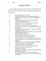
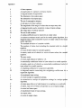
Appendix A Acronyms
46
Appendix B Symbols
47
Table Of Contents
1 iv
Appendix C Adjoint Derivations of the Recipe Update Equations
.50
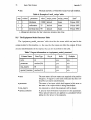
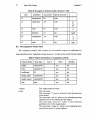
Appendix D Ingres Table Formats
52
Appendix E Alphabetical Library Function Listing
i50
Appendix F Description of the Source Files
'70
Appendix G Principal Library Functions Listed by Hierarchy
G. 1 The Beginning of the Program
G.2 Main BCAM Menu Actions
G.3 Activation of a Machine
G.4 Equipment Model Analyses
G.5 Workcell Operation
'7 5
'75
'7 5
'7 6
'77
'77
Appendix H Source Code Listings
Appendix I Known Bugs
Appendix J A G2 Formulation of Measurement Queuing Effects
J. 1 Introduction
5.2 Methodology
J.3 Results
5.4 Conclusions
5.5 Future Work
References
V
Acknowledgments
Acknowledgments
I
1
I cannot begin to express the magnitude of my appreciation and grat tude to my
research advisor, Professor Costas J. Spanos. His constant support and
invaluable to the success of my studies. I also thank Professor Seth
1
my dissertation committee. In addition, I thank Dean David A. Hodges for is profound
advice to me during both my undergraduate and graduate studies, and also fo his support
and leadership of CIM research at Berkeley. I am also most grateful to Profe sor Eugene
Wong, Professor Martin Graham, Dr. Sheila Humphreys, Winsor Letton, Dr. Shahab
Shiekholeslam, and David Wagner for their sage counsel through my years at berkeley.
For their generous assistance in the proofreading of this thesis, I thankiDr. Shahab
Shiekholeslam, Donald Zwakenberg, Sherry Lee, Eric Boslun, Sovarong Lea@, and John
Thomson.
I am also most appreciative of the efforts of Professor Gary May for his development
of equipment model structures and his work on the BCAM LPCVD diagndstic system,
Hao-Cheng Liu for his development of an equipment recipe editor, the BCAM diagnostic
system and the database tables used by the BCAM Environment, Edward h e n for his
work on statistical process control and response surface plotting, Sovarong Qeang for his
experimentation and development of photolithography equipment models and alarm
generation algorithms, Sherry Lee for her work on the BCAM diagnostic gystem, Eric
Braun for development of the BCAM response surface plotting application, q i - M i n Ling
for his development of microprocessing equipment models, and Lauren Masda-Lochridge
for her plentiful assistance with the Ingres database software.
During my years at Berkeley, my participation on the 155 crew team ha4 a profound
effect upon my studies. The training assisted my development in all aspects
01 my life. At
the heart of my rowing experience was my coach Jeff Wilk. His inspiration 8nd spiritual
Acknowledgments
vi
guidance gave me strength which allowed my studies to flourish. I must also acknowle !F
my teammates whose camaraderie and efforts contributed to my rowing experiences.
Also essential to the success of my research here at Berkeley have been the o er
members of the C I W C A M groups at Berkeley: Professor Lawrence Rowe, Raym id
Chen, Haifang Guo, Annika Rogers, Steven Smoot, Kwan Kim, Zeina Daoud, Mc di
Hosseini, and Soheila Bana.
I give my special thanks to Carol Block, Christopher Hylands, Ken Nishimura, Kat in
Voros, Bob Hamilton, Genevieve Thiebaut, Heather Brown, Cheryl Craigwell, and le
staff of the Berkeley Electronics Laboratory for their continual assistance in a multitud of
matters during my stay at Berkeley.
For their unfailing support and knowledgable advice throughout my life, I am etern
grateful to my parents John and Barbara Bombay, my sister Helen Bombay, ‘Y
grandparents Hunter and Annie Flores, and my cousins Michael Minatrea, Jeannie id
Joseph Miller, John Minatrea, Richard Buford and Janine Minatrea, and the rest of
lY
family. It is the great devotion and generosity of my family whom I must credit for a1 of
my successes.
I thank the National Science Foundation for their support of my graduate studie at
Berkeley. I thank also the Regents of the University of California, the Alumni Associa in
of the University of California, Warren Dere, and Edward F. Kraft, and Cornel1 C. M er
for their support of my undergraduate studies.
This research has been jointly sponsored by the Semiconductor Research Corporat In,
the National Science Foundation, Texas Instruments, National Semiconductor, and le
California MICRO program.
1
Chapter 1
Introduction
Chapter 1 Introduction
X
Until recently, IC fabrication facilities have relied mostly upon human e perience to
develop equipment recipes through trial and error. But as today’s designs push the borders
a
of existing technology, even the slightest maladjustment in equipment can drastically
undercut production. The industry has therefore experienced extremely long st rt-up times
when bringing a new product into regular production and costly cuts in production when
maintaining or replacing manufacturing equipment. This problem is further cbmpounded
by frequent unanticipated changes in equipment performance. Today these dhanges are
identified through Statistical Process Control (SPC), and sometimes a human operator
9’
attempts to re-adjust the process. Integrated circuit manufacturing tech ology can
therefore reap great benefit from the application of a more advanced control system.
A control system which can meet the stringent demands of IC fabricatibn must be
rather sophisticated. Simple feedback control applied to individual machines i6 unreliable
due to the low inherent capabilities (the ratio of specification limit ranges to noise
, standard
error) of the individual steps. A fabrication line control system must therefore have a solid
base in statistical analysis of equipment performance. A control system must @sobe able
to predict the equipment performance and adjust equipment settings whenever the
predicted performance deviates from specifications. In order to establish this capability, a
control system must use some sort of equipment models. Furthermore, in order to
compensate for equipment changes, the models must allow themselves to be updated
according to current manufacturing conditions. Statistically based models a e desirable
because analysis of equipment performance through regression techniques w 11 allow the
models to be updated efficiently.
Chapter 1
Introduction
2
The implementation of the control sclleme includes regular checks of equipml It
models and recalculation of appropriate machine settings whenever those models
e
updated. This is the feedback portion of the controller. Whenever a process consists If
several interdependent steps, e.g. the photolithography workcell, feed-forward cont ,1
may be implemented to compensate early deviations in equipment performance Y
adjusting the settings of subsequent processing steps.
So that this control scheme may be integrated into the factory environment, it inter2
Ls
with a database facility to store measurements and maintain a record of control recipes i d
equipment models. In addition, the control environment includes interfaces to ala n
generation, diagnosis, and statistical process control applications.
The implementation of this control environment and the underlying analysis functii 1s
have been realized using C++ and X windows. This realization is named the Berke Y
Computer Aided Manufacturing (BCAM) Control and Monitoring Environment an( is
described in this thesis.
After this introduction, the thesis devotes a chapter to the mathematical theory beh d
the controller’s model update and recipe update algorithms. This is followed by a chaI :r
describing the implementation of the BCAM environment. The BCAM user’s manual : d
the BCAM programming manual constitute the next two chapters. Finally, the conclusi
of this thesis are presented, and the possibilities for future development are discussed.
IS
3
Theory of Discrete Process Control
Chapter 2
I
Chapter 2 Theory of Discrete Process Contro
2.1
An Introduction to Discrete Process Control
The characterization of IC processes through equipment modeling
necessity in semiconductor manufacturing. Equipment models may be
or a combination thereof. Further, equipment-specific models are
the changing status of the equipment [7]. The Berkeley Computer-Aided Mabufacturing
(BCAM) group has developed several statistically based polynomial models that describe
the behavior of some important IC manufacturing equipment: the Tylan lob-pressure
I
chemical vapor deposition (LPCVD) furnace, the Lam plasma e t c h + - , and the
photolithography workcell [8][9][ 101.
The equipment models described in this work consist of mathematical expfpssions that
can predict the outcome of a manufacturing step (e.g. the thickness of the photoresist)
given the settings of that step (e.g. spin speed, spin time, etc.). Such models qre based on
the statistical analysis of the results of designed experiments; manufacturing ehuipment is
subjected to a well structured sequence of experimental recipes, and the resulting data is
analyzed through stepwise linear regression. This leads to models which accumtely reflect
the operation of the equipment. The development of these models is asisisted by a
theoretical understanding of the physical behavior of the equipment [3].
The basic equipment model has been designed as a polynomial expression with a
flexible representation so that it may operate efficiently within a comprehen$ive control
system. Several input and output transformations (exponential, logarithm, roqts, etc.) are
also supported.
I
Since equipment characteristics change with time, a complete model str cture must
allow for updates of the model. This is accomplished by means of creating n adaptive
Theory of Discrete Process Control
Chapter 2
4
model which has two parts: an original model which represents the original state of the
equipment, and a correction model which describes the deviation from that original stat?.
These models are used for performance prediction, the generation of descriptive
response surfaces, and other control needs. Given its prediction capability, the model may
also be used by optimization algorithms to deduce the required machine settings to m :et
target performance specifications. T h e optimization presented herein uses a
multidimensional Newton-Raphson algorithm subject to inequality constraints on the
machine controls.
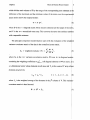
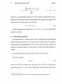
2.2 The Form of the Equipment Model
Initially, an equipment model is derived using a designed experiment.
model represents the general structure of the equipment behavior, i.e.
1
polynomial terms used in the model equation; these terms represent the ways in which he
machine’s settings influence its outputs. For example, such a model has been develo
for the photoresist spin-coat and bake equipment of the Berkeley
Laboratory [3]. The four settings of the machine are spin speed xl,
temperature x g , and bake timex,. The output is photoresist thickness
a representative model is
z =
Co
+ CIXz + C2X4 +
1
1
1
where the symbols c,, ...c j represent the coefficients of the terms of the model. Altho
the models are highly nonlinear with respect to the settings, they are linear with
the coefficients. This property allows us to use linear regression techniques to
the coefficients which best fit the machine in question. All equipment
general format, although the number of terms (and the form of those
machine to machine. Several transformations (such as the logarithm
5
Theory of Discrete Process Control
Chapter 2
1
are also supported on the inputs and outputs. As described next, the ada tive model
always retains the basic structure defined by the terms of its original model, lthough the
~
coefficients may be updated according to need.
2.3 The Model Update Algorithm
~
i
When, over time, a model fails to accurately represent a machine, correct ons may be
applied to the coefficients of the model. These corrections make up the
and are calculated by means of an update algorithm. The correction
with the original model make up the complete adaptive model. The m
algorithm is initiated by means of a statistical process control alarm which
whenever the machine outputs differ significantly from those predicted by
The model update algorithm is designed to modify the equipment model 4s necessary
during routine equipment operation. Using historical records from a machine$ operation,
,
the update algorithm performs statistical regressions to determine the optimuh correction
model. This algorithm performs well in either a single product or a mdlti-product
environment.
Because the adaptive model maintains a correction model while leaving /the original
model unchanged, it will never lose the information gained in the original designed
experiment. For example, a correction model may evolve to compensate dor a failing
machine part; when that defective part is replaced, the adaptive model can quickly
abandon the obsolete correction model and return to the original model.
Finally, each processing step has several outputs which can be controlled; hence,
several models must be used to describe each step. The spin-coat operation,
is characterized by the thickness and the reflectance of the applied
each output is represented by a separate model equation, the
each of these outputs separately.
Chapter 2
Theory of Discrete Process Control
6
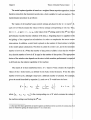
The model update algorithm is based on a weighted linear stepwise regression; it m Jst
therefore transform the historical records into a form suitable for such an analysis. Tiis
transformation procedure is as follows:
The values of the machine's past control settings are placed in the
K
x n matrix1 X,
each row of which contains the values of those settings corresponding to one run. This,
for k = 1.. .K and i = 1.. .n, xg is the value of the i* setting used for the k* run. Sir ce
performance records become obsolete with time, a forgetting factor is applied in the
weighting of the regression calculations in order to emphasize the most recdnt
t
observations. In addition, a strict limit is placed on the number of observations to incl de
in the model update calculations. This limit is called the window size, and is the maxim m
number of rows in X. (When the number of data points available is less than the wind w
size, then the number of rows in X is equal to the number of data points.) The appropri
choice of the window size depends on the rate at which machine performance is expec
to drift and also the inherent capability of the machine.
The matrix X is then transformed into a
Kx
t matrix
T that contains the
values of the t model terms, as defined by the basic model structure. T
number of rows as X,although it may have a different number of columns. For example,
given the model described by equation (l),each row of T would have the form:
tF
where [xk,
=
lk.2
xk, xk,
xk,4
1
&
1
Xk,3&
13
,
k = I...&
:2)
xk,l
43
xk, is the corresponding row of X which contains the values of
t
1. In this report bold-faced capital letters are used for matrices and bold faced lower case letters for column arrays. ow
arrays are obtained by applying the transpose operator CT) to a column array.
7
Theory of Discrete Process Control
Chapter 2
The update algorithm applies the current model (original model plus corr
to the machine setting corresponding to each run and predicts the respective
It then takes the machine’s corresponding historical output record z and
the vector containing the predicted output values, thus yielding the
vector A z . The elements of A z are defined by:
nt
where co is the current model’s constant term coefficient, and’c is the colu n vector of
1
the current model’s remaining term coefficients. This discrepancy vector wil be used in
order to determine the coefficients of the correction model.
The machine’s performance records have been transformed into the term matrix T and
the discrepancy vector A z . These data, however, are not the result of 8 designed
experiment, but rather the result of routine equipment operation; this fact Mill limit the
number of correction coefficients which can be evaluated. If, for example, the machine has
run with the same temperature setting throughout its relevant history, the data will not
contain any information to determine if the effect of the temperature setting hks changed.
Similarly, if all the machine’s settings have been held constant, then the correction model
should only include a correction to the constant term coefficient.
In general, the data may support a correction to some, but not all, of the coqfficients. In
order to determine which coefficients can be corrected and how to correct them, a
principal component transformation [6] is applied to the matrix T. This transfonnation has
the added benefit that the transformed data is also orthogonally distributed-a
property
which greatly facilitates the subsequent stepwise regression.
However, before executing the principal component transformation, the terms matrix
T must be properly numerically conditioned. This is accomplished by a tradsformation
Chapter 2
Theory of Discrete Process Control
8
which divides each column of T by the range of the corresponding term (defined as he
difference of the maximum and the minimum values of the terms over the experime :a1
space used to derive the original model):
4)
where D is the t x t diagonal matrix whose nonzero elements are the ranges of the ter
and V is the
K
IS,
x t normalized term array. This converts the terms into unitless numl rs
with comparable variances.
The principal component transformation starts with the evaluation of the weigl :d
variance-covariance matrix of the data in the normalized terms matrix:
Sv = weightedcovariance ( V ) =
v:. w -v,
U T -w - u
’
where S , is the t X t variance-covariance matrix, W is an K x K diagonal mat
containing the weighting coefficients
K
Wkklk =
(off diagonal elements of W are zero),
5)
X
is
a t-dimensional vector whose elements are all ones, and V , is the centered V array wk se
elements are given by:
5)
where V.j is the weighted average of the elements in thej* column of V . This variar
E-
covariance matrix is then factored:
7)
Theory of Discrete Process Control
9
Chapter 2
6.
where A is the t x c diagonal matrix containing the t eigenvalues of S y , and
is the t x t
orthonormal matrix' whose columns are the corresponding eigenvectors2 f S,. The
matrix BT is then used to transform V to its principal component space as foll
Vpc = V . B ,
i
where V,, has the same dimensions, n x t , as V and T,and it contains the nput terms
B
data transformed into the principal component space. The output discrepanci s may now
be represented by rewriting (3) as:
I
or equivalently:
k =
where
l.'..K,
(10)
vp,- are the rows of V p c ,and y = B T .D . c represents the vector Of the term
coefficients of the original model, transformed into the principal component sdace.
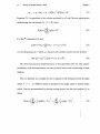
Next, a weighted stepwise regression is performed, considering each principal
component separately in order to obtain a model correction coefficient Ay[ ( I
= 1 .. .t ) for
that component. Only principal component directions showing significant variance should
be considered; therefore, the algorithm examines only the principal components whose
corresponding eigenvalues h, of S, satisfy the inequality
1 = l...t,
t?
(11)
where r is the magnitude of the range of possible values that the output may t e, and a is
a unitless empirical quantity taken to be
for the BCAM application. (T e factors in
1. An orthonormal matrix has orthogonal columns (and rows),each of which has a magnitude of one.
orthonormal matrix is simply its transpose.
e inverse of an
2. Because S, is symmetric positive definite, this factorization is equivalent to the singular value deco@position of S,.
Chapter 2
Theory of Discrete Process Control
(1 1) are necessary to ensure that both sides of the inequality have compatible units.)
each considered correction coefficient Ay,, a p-value' is calculated. If this p-value is
enough, the calculated value for that correction coefficient is accepted, Otherwise
correction coefficient is set to zero. The regression analysis takes the form of the syste
where A y is the column vector of model correction coefficients in the
component space. The significance of each correction coefficient is established
at the variance of each estimator. This variance is related to the standard
the machine output:
var(Ay) = [ VFc. W . V,,]
The standard deviation
CT
-2
[Vi,.
I$. V,,] . u
CT*.
is estimated from the residuals of the regression
the creation of the original machine model. Additional estimates of
CT
during replicated runs.
In order to ensure the stability of the algorithm, an additional test is applied to
extreme corrections to the model. During an update procedure, no model coefficient
change by more than 60% of its previous value.
Once all significant principal components have been examined, the terms array V ,
multiplied by the new correction coefficients Ayl, and the resulting vector is
from the output discrepancy vector Az. The weighted average of the
resulting vector, if significant, is the constant term correction coefficient
1. The pvalue is the probability of obtaining an estimate of the correction coefficient whose magnitude is greater
the considered estimate, assuming that the true value of the correction coefficient is zero. Typically, if the pvalue is
than 0.05, then the correction coefficient is accepted as significant.
1 10
11
Theory of Discrete Process Control
Chapter 2
.K,
(14)
Wkk
k= 1
w.The correction coefficients
:e then put
through the inverse transforms which bring them back into the original terms
lace, where
where the
Wkk
are the diagonal elements of
they become the correction model's term coefficients
AC = D - ' - B -Ay.
(15)
Finally the updated model coefficients are c + A c and co + A co, and the c )del update
procedure is complete.
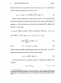
2.4
Recipe Update Algorithm'
The implementation of a feedback control system to integrated circuit manufacturing
requires that the controller be able to update machine settings whenever equipment
models change. The implementation of feed-forward control similarly rkquires the
calculation of machine settings. For these purposes, a settings recipe update hlgorithm is
required.
The unconstrained recipe calculation problem reduces to the following:
Solve for x such that
f ( x ) =2
where x
E
1
X c % n , the n-dimensional input space, 2 E Z c tKm, the rn-dimensional
output space, and f : X
+ 2.An iterative algorithm is presented which starts with an
1. Note that some symbols in this section do not correspond directly with those of the previous section
Chapter 2
Theory of Discrete Process Control
12
initial xo and generates a sequence x,,, xl, x2, ... converging to the best cornprom se
solution 2.Convergence properties of this method are discussed in [ 181.
Denote the j* component of f: as f ’ : X
+ 31. Then at each iteration k, f
can )e
linearized’ about x, to get
7)
where
This leads to the modified problem: find a compromise solution x,+ such that
9)
If n 2 rn and A A f is invertible, then a solution2 to this modified problem is
0)
Using a Euclidean norm, this solution is as close as possible to the previous solution xk If
n < rn and AIAk is invertible, then the least square error solution to the modified probl :m
is
1. The models used in the BCAM recipe generation algorithm are such that the solution to the modified problem (1 ) is
at each iteration close enough to the best compromise solution 2 , so that the sequence of solutions x,,, x,, x2, ... m-
verges to 2 . In general, the convergenceproperties of this method require hounds on the minimum and maximum si gu-
Jf
lar values of the derivative matrix ax
( 0 )
over X.
2. See Appendix C for a derivation of these equations.
Chapter 2
Theory of Discrete Process Control
13
(21)
Equation (21) is equivalent to the solution produced by a Local Newton c timization
method using the cost function G, : X
+ 3,where
m
G,(x)
=
[&x)
-21 ',
j = l
2' is the j* component of 2, and
(i.e. the linearization off
about x k ) .Equation (20) similarly results from the roblem
(24)
Of course any practical implementation of this algorithm must not c ly require
invertibility of the relevant matrices, but also put finite limits on the conditior ig of those
matrices.
The cost function G, is simply the sum of squares of the deviations fro& the target
values
f ,j
= 1...rn. Different scales of measure for the target values 2' and the recipe
values x'can be accommodated by placing scaling factors into the cost fun
obtain
Theory of Discrete Process Control
Chapter 2
where the d ( j = 1...rn) scale the target values' and R is a diagonal n x n mi
containing the scaling factors for the recipe values2 so that y
and
E R-'x.
Thus &)
=g
h)= m y ) .
Let
-Ak-R,
2k'S-l
where S is the rn x rn diagonal matrix containing s', j = 1...rn. This leads to
following modified equations3
where
6Zk
=
fot,> - 2 .
Thus the new problem at iteration k is
min
{Gk(y) I ~y
E
XI.
-
If n = rn and A k is invertible, then the solution to (29) is
-
-T
If n > rn and AkAk is invertible, then a solution to (29) is
-1
Xk+ 1
=
Xk
+ Axk = X k -RA:[AkAy s-' I f ( X k ) -21
,
1. For the calculation of machine settings, s' = 2 . min(USL' - target', target' - LSL')
2. For the calculation of machine settings, is the range of valid scttings for control i, Le. the maximum valid 1
value minus the minimum valid setting value.
3. The notation (., ) represents the scalar product.
Theory of Discrete Process Control
15
and this solution as close as possible to the prcvious solution
xk.
i
Chapter 2
-T-
If n < rn nd A k A kis
invertible, then the least square error solution to (29) is
si
Because the above algorithm uses approximations to f ( * ) , a more robu t algorithm
uses the above equations to calculate a search direction hk (in equations (30) through (32)
e
substitute xk+ by hk),and then uses an Armijo step size algorithm [20] to d termine the
,
actual A x k = h,h,, where
zx{7
...
1
L
1Cfj(Ry)-z/] } ,
(34)
;= 1
so that
(35)
Whenever there are problems with performing the matrix inversion in (30), (3 l), or (32), a
steepest descent method can be used to find thc search direction':
For most systems, the set of valid input rccipes X is constrained. Consiider a set of
constraints
i = l...n
report.
(37)
Chapter 2
where x
Thcory of Discrete Process Control
~is the
~ minimum
,
~ valid value for setting i, and x
16
~is the
~ maximum
,
~ vi id
value for setting i. Whenever a recipe is calculated, the algorithm must be able to rem in
within the constraints given by (37). To handle these constraints, a feasible modificatil 11
to the above algorithms freezes any constraint violating input value (at the minimun or
maximum according to the nature of the violation), and reduces the dimension of the in ut
space by one. Thus the optimization can continue with the remaining inputs. For a m re
robust system, a more general constrained optimization algorithm could be applied [20
1. The reliability of this modification -;pen& on the assumption that all of lhc modeled output values are monotoni JlY
either increasing or decreasing with respect to each individual setting value, an assumption which is satisfied by ost
semiconductor processing equipment.
17
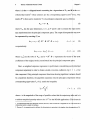
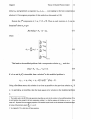
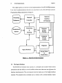
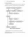
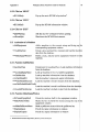
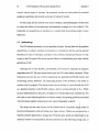
2.5
Theory of Discrete Process Control
Chapter 2
Application of the Model Update and Recipe Update Algorithms
The presented methods for checking and updating equipment
calculating a new equipment setting recipe are built into the BCAM
The model update algorithm is used as part of the feedback system
models for processing equipment. The recipe update algorithm
purposes; it is used for initial setting calculations, for recipe
equipment models change, and for feed-forward cdculation of workcell contr 1s.
(i
Recipe
Update
Wafers
I
1
I
Model
Update
I
BCAM Implementation
Chapter 3
18
Chapter 3 BCAM Implementation
3.1
Introduction
Because the accurate control of manufacturing processes is critical to the producl in
of integrated circuits, a control scheme is needed so that deviations from prod ct
specifications may be compensated by automatic adjustments to the process. This con 31
must exploit the interdependence of the various steps involved in production. Software
IS
been developed to utilize equipment models for supervisory control. The software uses le
models for process simulation and recipe generation. This recipe generation is use(
:0
accommodate product specifications and to implcmcnt ked-forward control; in orde
:0
compensate for deviations in the middle of a process run, fced-forward control adjusts
le
settings of subsequent process steps.
Feedback control is initiated by a model-based control and monitoring schei e.
Alarms using statistical analyses [5] are employed to detect consistent departure: .n
equipment performance from the performance predictcd by the equipment models. 0 :e
this departure has been established, the model is modified through a model upd te
algorithm [7] and the equipment control settings arc correspondingly adjusted. 1 .e
workcell controller has several process analysis functions which examine equipm n t
interconnection information to determine the order of processing steps, to prec st
performance of an entire workcell, and to perform sensitivity analyses on the workc 1.
Feed-forward control is initiated whenever the projected properties of a wafer lot
11
outside of specifications. It is implemented by adjusting the recipes (control settings If
subsequent processing steps. If projections predict that fecd forward control cannot bi 'g
the lot back within the acceptance limits [13], the lot will be discarded or re-processed
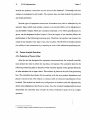
19
Chapter 3
BCAM Implementation
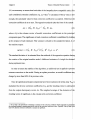
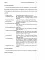
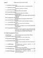
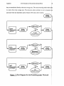
This chapter gives an overview of the implcmcntation of the BCAM E
L o w level implementations details are described in the B C A M
Programming Manual presented in Chapter 5.
,t 4Fp
Statistical
Diagnosis
I
Ingres Database
Recipe Editor
&
Model Editor
e 2 TheBCAMEnviro-
3.2
The Ingres Database
The BCAM environment must operate in a multiple user system with security
1
precautions and the ability to avoid conllicts when more than one user ccesses the
database simultaneously. The environment therefore makes use of the Ing es database
program. This program allows multiple users to interact with a central database. Ingres
Chapter 3
BCAM Implementation
20
also allows different levels of permissions, such as those of an operator or an engineer.
Ownership and time stamps are maintained for all tables stored in the database, there by
preserving security and preventing access conflicts. Thc BCAM Environment uses Ingres
library functions to store and retrieve equipment recipes and models in the database. In
order to enhance the portability of the BCAM Environment, the code has been developed
to allow easy modification for use with other databasc programs.
3.3 The Role of X Windows in the BCAM Environment
The X window system provides a means to implcmcnt an aesthetically pleasing, user
friendly interface to the BCAM environment. X windows were chosen because they ixe
available throughout the industry and are standardized to work on most workstations, A
commercially available graphical interface packagc was also investigated, but it was
determined to be inappropriate for the BCAM Environmcnt. This study is described in
Appendix J.
3.4 Operations on Indihdual Machines
The most basic function of the BCAM environmcnt is the selective activation of
individual machines. Once activated, the BCAM system can interact with each machine: in
a variety of ways.
By accessing the system database, a recipe editor' allows machine settings to be
retrieved, edited, and saved as desired. Ownership and time stamps are maintained on all
recipes. Recipes may also be calculated to meet specified targets.
Analytical models f o r the machine are also loaded from the database. T h e
implementation allows full interaction with these models, including editing, automz.tic
model updates, response surface viewing, and storage of all models in the database. As
1. The recipe editor has been developed by Hao-Cheng Liu of the Bcrkclcy Computer-Aided Manufacturing group.
21
BCAM Implementation
Chapter 3
N
models are updated, corrections are also stored in the database’. Owners ip and time
a
stamps are maintained on all models. The operator may use these models f r prediction
and recipe generation.
l
1
Several types of equipment connection information may also be addr ssed by the
operator. Inputs which must remain constant or are uncontrollable can be d signated as
uncontrollable. Outputs which are considercd important, or for which speci cations are
given, can be designated asBnal outputs. Often the output of one machine affects the
I
performance of the following processing step. Therefore, the operator can /connect the
t”
of the addressed inpu4output pair.
output of any machine to the input of any othcr machine. The BCAM environ ent checks
for validity of such connections by comparing thc units
3.5 Process Analysis Functions
3.5.1 Deduction of Process Order
After the user has designated the equipment intcrconnections, the workcall controller
must deduce the order in which the machines will operate. The controller does this by
following connection paths to determine which machine depends on the greatqst hierarchy
of other machines for its input values. This machinc is placed at the end of th$ processing
line. The controller then checks for the machinc with the next greatest depqndence and
places it second to last. The method is continued until all connected machin
1
have been
included. This method can handle any conligurcltion of machines and will a tomatically
detect misconfigurations which lead to loops. Once the workcell configurati n has been
determined, the controller may consider thc wholc workcell (or parts of iti as a single
operation.
1. Automatic storage of model corrections has not yet hwn implcmented.
Chapter 3
BCAM Implementation
22
3.5.2 Workcell Performance Prediction
For several applications, the workcell controller must be able to predict the fi
outputs of a workcell based on the individual controls applied to all machines in
workcell. This is accomplished by first predicting the outputs of the first machine, feed
these outputs to the inputs of the following machinc, and continuing until the predicti
for the last machine have been calculated, thus yielding the desired result.
3.5.3 Workcell Sensitivity Analyses
In order to determine the sensitivity of any workcell final output to any workcell in]
the controller uses a recursive algorithm. This algorithm uses the workce
interconnection information to implement a multidi mcnsional evaluation of differential
of composed functions. The level of hierarchy for thc composition (and thus the leve
recursion) depends on the number of machines bctwccn the machine receiving the in
and the machine whose output is considered.
3.6 The Workcell Operations
In addition to providing control over a processing line, the controller must be ablc to
conduct simulations of the process. This will allow opcrators to perform preliminary ti StS
of new process configurations or control schemes without expensive and time consum ng
wafer processing.
The run-by-run control system under development by the BCAM group uses moc 9s
for the individual machines in a process to build a model o C the entire process. A proc :ss
specifications menu enables the user to set the product's desired characteristics, and t en
the controller will automatically calculate the optimum equipment settings to meet 1 iat
product's specifications. These settings make up thc process recipe. Once this has b en
accomplished, the controller may begin processing wafers.
23
BCAM Implementation
Chapter 3
6
As wafers are processed, the BCAM Environment makes a record of eac machine's
performance. This record is used by the alarm generation module, the m del update
algorithm, and the graph generation module.
3.7 The Interface to Other BCAM Applications
i
0
The Berkeley Computer-Aided Manufac luring research group has devel ped several
applications for manufacturing. These applications can be invoked for use w i k a piece of
equipment through the BCAM environment.
I
Formal alarm generation algorithms have bccn developed by Sovarong p a n g [22].
I
They will be integrated into the monitoring systcms of the BCAM environmedt.
i
Real time statistical process control (SPC) algorithms have been imp1 mented by
Eddie Wen [22][23]. This implementation includes graphical displays. The SPC
application functions for measurements taken from the Berkeley Micrdfabrication
Laboratory's Lam Autoetch 490.
An application which performs diagnoses on equipment malfunctio& has been
1
developed by Dr. Gary May, Hao-Cheng Liu, and Sherry Lee [16][17]. Th s diagnosis
I
module is available for the Berkeley MicroPabrication Laboratory's Lam iAutoetcher
through the BCAM environment.
An application to create two and three dimensional response surface plots of
equipment models has been developed by Eddie Wen and Eric Braun for use with the
BCAM environment' ~221.
,
~
1. This model plotting algorithm is currently in the proccss of inkgration into the BCAM environment.,
BCAM 13nvironment User’s Manual
Chapter 4
24
Chapter 4 BCAM Environment User’s Manual
4.1
Introduction: Starting the BCAM System’
To enter into the BCAM environment, first change directories to “-bcamdev/t
7”
then enter the command “source -bcam/src/main/.bcam” and then enter the comm, id
‘‘./BCAM”
An introductory widow will appear. Click on “Ok” to continue. At this point the n: in
menu will appear. To activate some equipment, click on the “EQUIP” selection and a ml
IU
of available equipment will appear. Clicking on an equipment name activates 1 at
equipment, and a window for the equipment will appear. Several machines may
3e
activated at any given time.
The individual equipment windows allow a multitude of operations. Equipment set1 ’g
recipes may be edited, stored, and retrieved from the BCAM database. Simila Y,
equipment performance models may be edited, stored, and retrieved. The equipm nt
window also facilitates the definition of equipmcn t interconnections for use with ie
BCAM workcell controller application. In addition to the workcell controller, the BCA M
environment supports Diagnosis and Statistical Process Control (SPC) applications; tk se
applications are also activated from the equipment window.
1. These instructions are for the current experimental implementation on 11. C . Berkeley’s radon Sun4 computer.
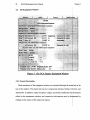
25
4.2
Chapter 4
BCAM Environment User’s Manual
The Equipment Window
e 3 The GCA SteaQer Eqybment Windoq
4.2.1 General Description
Most operations of the equipment window are accessed through the medu bar at the
top of the window. This menu bar has four components: Recipe, Model, Connect, and
Application. In addition, values for inputs, outputs, and model coefficients may be directly
edited in the equipment window, and connection information may be de$ignated by
clicking on the names of the inputs and outputs.
I
Chapter 4
BCAM Environment User’s Manual
26
4.2.2 The Equipment Recipe Menu
The Recipe Menu is used to access all functions associated with the currently sto ed
recipe of control and input values for a machine. The machine is also deactivated throi gh
this window.
0
0
0
0
0
Load Recipe...-Select and load a recipe from the BCAM database.
Load Default Recipe-Load the user’s default recipe from the BCAM database; if he
user has no default recipe, the BCAM system default is loaded.
Save Recipe-Save the current recipe into the BCAM database under the current n a le.
Save Recipe As...-Specify
a name for the current recipe and save it into the BCt ,M
database.
Restore Recipe-Restore the recipe to the values it had at the last operation.
Delete Recipe-Delete a recipe from the database.
Output Targets-Set target values and tolerances for all final outputs of this machint
Output Specifications-Set target values and specification limits for all final outpuu of
this machine.
Calculate Recipe-Generate a recipe to produce the final output values specified by
targets.
Download Recipe-Download a recipe of controls to the physical equipment.
Deactivate this Machine-Eliminate this equipmcnt window and deactivate he
corresponding machine.
4.2.3 The Equipment Model Menu
The Model Menu is used to access all functions which deal with equipment models
Load Model...-Select and load a model from the BCAM database.
Load Default Model-Load the user’s default model from the BCAM database; if .he
user has no default model, the BCAM system default is used.
Save Model-Save the current model into the BCAM database under the current n a le.
Save Model As...-Select a name for the current model and save it into the BCt LM
database.
Display Original Model-Display the model as it existed before any feedbi ck
corrections.
Display Current Model-Display the current adaptive equipment model (origi la1
model plus correction model).
Confirm Current Model-Confirm the currently edited and displayed model and tak :it
as the current adaptive model.
Predict-Predict the outputs generated by the current input recipe.
27
BCAM Environment User’s Manual
Chapter 4
I
Check Model-Using equipment performance data, execute statistical re ressions to
check (and if needed, correct) the current adaptive model.
Response Surface Plots-Activate the response surface plotting facility fo equipment
models.
Load Simulator Model...-Select
and load a simulator model from he BCAM
database.
i
Load Default Simulator Model-Load the simulator with the user’s
the BCAM database; if the user has no default model, the
used.
Display Simulator Model-Display the model currently
equipment simulator.
Confirm Simulator Model-Confirm the currently edited
it as the current simulator model.
Note that there are two distinct models used in the
P
the current (controller) model. This model is used for all prediction and contr 1 purposes,
including the feedback and feed-forward control algorithms. The original vedsion of this
controller model is also maintained and may be viewed with the Display Ori$inal Model
command. The Check Model command is used to manually initiate a check arid update of
this model. The other model is the simulator model; this model is usedl purely for
demonstration purposes. Unless the simulator is explicitly specified, all ref&rencesto a
model are to the controller model.
4.2.4 The Equipment Window-Dejning Equipment Connections
To connect the input (setting, control, or incoming measurement) of onelmachine to
the output (usually a post-processing measurement) of another machine, click
I
successively upon the appropriate input name and output name. The display will then
change to describe this connection. To remove the connection, click upon the name of the
input side of the connection (i.e. where that paramekr shows up as an input).
For control purposes, not all outputs are critical to the final product of
To designate an output value to be of final importance, double click upon
output. The window will then show that output to be a “final output.”
Chapter 4
B C M Environment User's Manual
28
automatically prompted for specifications whenever a linal output is designated. Anol ier
two clicks upon the output name return the output to normal status. Multiple final out1
Uts
may be designated.
In many cases, input parameters which affect machine performance may no1 be
controllable. Furthermore, it may sometimes be desirable to hold specific machine con rol
inputs constant. In such cases, the relevant inputs may be designated as uncontrollable To
declare an input uncontrollable, double click upon the name of the input. The display d l
then reflect this designation. Another single click revcrscs the designation.
Because the workcell configuration depends on cquipment interconnectic
IS,
connection information may not be changed while the BCAM Workcell Controlle is
active.
4.2.5 Example: The Interconnection of a Photolithography Workcell
The following figure shows a photolithography workcell using three piece: of
equipment. Two measurements are taken on the wafcrs exiting the photoresist spini er:
photoresist thickness (T) and reflectance (R). Thc photoresist reflectance is ag iin
measured after exposure (the thickness is not affcctcd'by the exposure). Finally, he
critical dimension (CD) is measured after the devcloprnent. Since the thickness nd
reflectance measurements are considered inputs to thc following processing steps (t eY
appear in model equations used by the BCAM controller), they are connected as depic ;ed
Chapter 4
f
3
Eaton
Photoresist
SP’
inner
R . R
f
GCA
Photoresist
Exposure
R
v
R
MTI
Photoresist CD (fin
Developer
output),
r
Once the three machines have been activated, the following sequence of
ouse clicks
will set up the connections in the BCAM environment:
Double click on the developer’s output CD to dcsignate the final output.
Click on the developer’s input thickness, and click on the spinner’s output thickness to
connect.
Click on the exposure’s input thickness, and click on the spinner’s output thickness to
connect.
Click on the developer’s input rcflcctancc, and click on the exposuke’s output
reflectance to connect.
Click on the exposure’s input reflectance, and click on the spinner’s output reflectance
to connect.
The workcell connection information is thus completed. The workcell controller may
now be invoked through the Equipment Applications Menu described in 4.2.7.
4.2.6 The Equipment Connections Menu
Connect Input-Change the status of an input or connect the input to the output of
another machine.
Connect Output-Xhange the status of an output or connect the output to ‘the input of
an0ther machine.
Chapter 4
BCAM 13nvironment User’s Manual
30
4.2.7 The Equipment Applications Menu
This menu is used to access other major BCAM applications.
Workcell Controller-Activate the BCAM Workcell Controller using curr
equipment interconnection information. (see below ‘The Workcell Window’)
Statistical Process Control-Activate the BCAM Real-Time Statistical Process Con
monitoring system [22][23]. This application is not available for all machines.
Diagnosis-Activate the BCAM Diagnosis module [ 161[ 171. This application is
available for all machines.
Response Surface Plots-Activate the response: surface plotting facility for equipm
models [22].
nt
01
ot
nt
4.2.8 The Equipment Window-Editing Values
The values shown for input values, output values, and model coefficient values re
editable. To edit these values, click the mouse pointer upon the value to be edited.
le
value may then be changed using the usual editing keys. All commands from le
equipment window check these editing fields for ncw values before executing.
le
workcell controller, however, does not automatically check model coefficient values, id
it is therefore desirable to manually confirm these values (from the Model pulldown me u)
after editing. This is necessary, for example, whenever the simulator model is changed
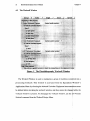
31
4.3
BCAM Environment User’s Manual
Chapter 4
The Workcell Window
re 5 ThePhotoli t h o w h v Workcell Window
The Workcell Window is used to manipulate a group of machines connkcted into a
processing workcell. This window is activated from the Equipmenti Window’s
Applications Menu by choosing the Workcell Controller. Equipment interconn
be defined before invoking the workcell window, and they cannot be chang
workcell window is present. To disengage the workcell window, use the
Workcell command from the Workcell Recipe Menu.
BCAM Environment User’s Manual
Chapter 4
4.3.1 The Workcell Recipe Menu
32
.
This menu accesses functions for manipulating workcell recipes. The Workc ?11
Window is also disengaged through this menu. In addition, this menu can be used to
specify target values for the final outputs of the workcell. Upon receipt of he
specifications, the controller automatically attempts to calculate a recipe of controls wh ch
will yield the desired results.
Edit-Edit
the current workcell controls.
Load...-Load
a new recipe for the workcell controls from the database.’
Load Default-Load default controls for the workcell
Save-Save current controls into the database.
Save As...-Save current controls under a specified name.
Final Output Targets-Specify final output targets and tolerances.
Final Output Specifications-Specify final output targets and both upper and 107 rer
specification limits.
Calculate Recipe-Calculate a recipe to meet output specifications.
Exit Processing Workcell-Exit the workcell mode and Workcell Window.
4.3.2 The Workcell Wafer Menu
This menu is used to initiate actions upon or about wafers, including actual operat on
of the workcell.
Run Wafer Through Workcell-Send a wafer to the workcell for processing.
Simulate a Wafer Run-Simulate the workcell’s operation on a single wafer (used For
demonstration).
Simulate N Wafer Runs...-Simulate a series of wafers through the workcell (used for
demonstration).
Predict Final Outputs-Predict the final outputs of the workcell using the curr :n t
recipe.
Sensitivities-Display the sensitivities of the final outputs to the workcell’s controls 2
Evaluate Cpk Capability-Evaluate the Cpk capability of the ~ o r k c e l l . ~
1. Database operations for the workcell have not yet been implemented. These operations are, however, available rom
the individual equipment windows.
2. Sensitivity displays have not yet been implemented.
3. Cpkevaluation has not yet been implemented.
BCAM Environment User’s Manual
33
4.3.3 The Workcell Graph Menu
Chapter 4
1
This menu accesses the graphical utilities associated with workcell operatihn.
1
Outputs-Graph the recorded output measurements of all workcell machin s.
Final Outputs-Graph the final output measurements of the workcell.
Prediction Errors-create regression control chart on prediction errors.
Autocorrelation-Graph the autocorrelations of prediction errors.
CUSUM-Show a CUSUM graph of final output measurements.
Inputs-Graph the controls used versus wafer numbers.
Normalized Inputs-Graph all inputs normalized to fit on a single graph.
I
Adaptive Models-Graph the coefficients of the adaptive models.
4.3.4 The Workcell Alurm Menu
This menu is used to access BCAM alarm utilities. Manual alarms can be $sued using
this menu 1.
Invalidate History-Specify that all previously recorded measurement$ should be
ignored by the model update algorithms.
Discard History-Purge all recorded measurements from memory.
I
4.3.5 The Workcell Options Menu
The workcell controller allows the user to specify several optional parameters for
dealing with the workcell. These parameters are accessed through the Workaell Options
Menu.
Turn Ordoff Feed-Forward Control
Turn OrdOff Feedback Control
Turn Ordoff EVO$
1. This menu will be expanded in the future [22].
2. Evolutionary operation has not yet been implemented.
Chapter 5
BCAM Environment ProgrammingManual
Chapter 5 BCAM Environment Programming Manual
5.1
Introduction: The Basic Program Structure
To aid in the ongoing quest to improve integrated circuit manufacturing techniqu s,
the BCAM group has developed an object-oriented software library describing 1 Le
fabrication equipment. The library provides a set of functions for interacting w ;h
equipment and databases and for manipulating various models of machine performan1 e.
Once the BCAM software has loaded equipment information into memory, it can perfo n
predictions, sensitivity studies, simulations, recipe generation and statistical proct
;S
control. Also included in the software arc procedurcs for updating machine performar :e
models, alarm generation, and diagnostic analyses. The BCAM software is organized a a
library which can be accessed by all modules in the BCAM architecture (e.g. workc 11
controller, recipe editor, malfunction diagnosis, and statistical process control). The ent :e
library is written in C++, an object-oriented superset of the C programming language. C
.+
extends the normal capabilities of C by adding features such as data abstraction, messal :passing, polymorphism, inheritance, and class hierarchy [ 111.
The BCAM environment is built around a C++ class called machineCZass. This d; ta
structure includes all the information necessary to interact with the physical machii
Y.
I
Member functions of this class or its member classes are used for BCAM actions relal :d
to the individual machine. For every equipment activated, a separate instance o a
machineCZass structure is created. When the BCAM Environment is active, ea h
machineCZass structure manifests itself on the screen in an Equipment Window.
Although the greatest care has been taken to keep this information current, herein m
be discrepancies with the current code. For the most recent information, please refer to 1
source code.
BCAM Environment Programming Manual
35
5.2
Chapter 5
The Creation of the Main Windows
The program first creates an entrance window which introduces the operator to the
system. When the operator is ready to begin, a mouse click will bring up the main menu
f o r the environment. T h i s main menu i s created using t h e f u n c t i o n Widget
MakeMainMenu(). Callbacks are set up from this menu to access the highest level
operations, most importantly the activation of equipment. The functions w iich handle
these actions are located primarily in the files ‘controllerEntrance.cc’, ‘equ..pSetup.cc’,
and ‘mainMenu.cc’.
4
Whenever a machine is activated, an instance of machineClass is reated and
information from the database is loaded into this structure. Then a calh to Widget
machineClass::MakeEquipWindow() creates the actual equipment window. Initegral in the
creation of the equipment window is the creation of the bar of pulldown menus from
which most operations are accessed. This is accomplished through use of the functions
Widget MakePulldownBar() and Widget MukePulldownMenu(). The functions which
handle these actions are located primarily in the files ‘equipWindbw.cc’ and
‘mainMenu.cc’ .
The workcell controller window is created in a similar fashion to tha equipment
window. The functions which handle these actions are located primarily1 in the files
‘process.cc’ and ‘mainMenu.cc’.
5.3 Naming Conventions
Except in cases of imported code, the following naming conventions have been
adhered to:
Macro names are all capital letters (e.g. MACRO).
Function names are lower case with all individual words beginning with c
for ease of reading (e.g. FunctionName).
BCAM Environment Programming Manual
Chapter 5
8
8
8
36
Variable names (except for those of Widget type) are lower case with imbedded wc -ds
beginning with capital letters for ease of reading (e.g. variableName).
Variable names of type Widget are lower case with imbedded words separated by he
underscore character (e.g. widget-variable-name).
Type and class names follow the same conventions as variable names.
5.4 Source Code File Hierarchy
The source code file hierarchy (from top down) is approximately organ zed in he
following order:
BCAM.cc controllerEntrance.cc
mainMenu.cc
equipSetup.cc
machineRW.cc
modelRW.cc
modelIngres.scc recipeIngres.scc
equipWindow.cc functions.cc messageWidget.cc makeWarning.cc
connections2.cc connections.cc modelChoice.cc
process.cc interfaces.cc .
generateRecipe.cc
modelUpdate.cc
graphsBCAM.cc graphRM.cc
diagnosis.cc
modelEval.cc
steps-cc
modelSpecFn.cc
mymath-cc
'
37
Chapter 5
BCAM Environment Programming Manual
5.5 Structure Declarations
Descriptions of most data classes and thcir mcmber functions are conti ined in the
declarations file ‘machineTypes.h’.The principal classes have the following hi :rarchyl :
historyClass
historyClass
inputclass
inputclass
1
inputStepValueClass
inputStepValueClass
connectionClass
t
outputclass
outputclass
Figure 6 BCAM C++ Data Structures
The principal members of some of the important structures are as follows:
d
1. Arrows indicate pointers (horizontal arrows form linked lists); vertical bars indicate membership: an horizontal bars
indicate consecutive members of an array.
Chapter 5
BCAM Environment Programming Manual
I8
5.5.1 class machineclass
The core of the BCAM environment is the class machineclass. It has many mem :r
data structures and functions, only the most important of which are described here. Sa le
of these members are themselves classes, and these classes are also described in
1
is
document.
The equipment window displayed on the screen.
The current models for machine performance. Incluc
a r e the models both for control purposes and
simulation.
A linked list of historical equipment performance data.
historyClass* history
The identification number of the wafer currently be
int waferNum
processed by this machine.
int GetInputIndex(char* inputName)
Return the array index (into modeZ.inputs) of the in
named inputName.
int GetOutputIndex(char* outputName)
Return the array index (into modeZ.outputs) of the out
named outputName.
double predict(int outputNum)
Evaluate and return the value predicted for output num
outputNum using the controller machine performai
model and the current rccipc for inputs.
Simulate all outputs of this machine including Gauss
void simulate()
noise. Simulated o u t p u t v a l u e s a r e s t o r e d in
model.outputs array.
Look at the historical pcrformance data of this mach
int ModelUpdate()
and determine if an update to the machine's contro
model is statistically justified. If a correction is justifiec
is made, and the function returns a positive val
Otherwise the function returns zero. A negative ret
value indicates an error.
machineclass* next
A pointer to the next machine in the linked list
machines.
Widget window
modelClass* model
d
)r
It
It
:r
m
e
n
e
le
:r
it
d .
s
'n
)f
5.5.2 class modelClass
This class contains most of the information ncccssary for modeling or simulatin a
machine's performance.
Chapter 5
BCAM Environment Programming Manual
39
char* equipName
char* formalName
The abbreviated name of the machine.
The formal name of the machine
~
~
The login name of the current BCAM user.
A matrix containing the exponents for the inp ts in all the
terms used in the equipment model. Each row orresponds
to one term. Column indices correspond to inp t numbers.
This member is private.
A matrix containing special function codes fo the inputs
int** s p e c 3
in all the terms used in the equipment mode . Each row
corresponds to one term. Column indices co espond to
input numbers. The code zero indicates tha no special
function is to be used. Special functions ard applied to
inputs before cxponcnts. This member is privak.
inputclass inputs[MAX-INPUTS]
The array of input descriptors of the machine. khe current
recipe is located within.
I
The number of inputs for the machine.
9 int input-cnt
outputClass outputs[MAX-OUTPUTS]
Thc array OK output descriptors of the machine,
The number of outputs for the machine.
int output-cnt
double simulate(int outputNum)
Simulate and return the value f o r o u t p u t number
outputNum using the simulator performancei model and
the current recipe for inputs.
double predict(int outputNum)
Predict and return the value of output numberloutputNum
using the controller’s current adaptive model and the
current recipe for inputs.
9
char* user
double** exp-mat
1
9
5.5.3 class processNode
Another important class is the class processNode. This class is used tol describe a
workcell containing several machines. This class is used extensively by ithe BCAM
Workcell Controller. W h e n the workccll controller is invoked, th/= machine
interconnections are analyzed and a linked list oKprocessNodes are created to bescribe the
order in which the machines operate, i.e. describe the process. Each process dode has the
following members:
BCAM Environment Programming Manual
Chapter 5
40
muchineClass * machine
A pointer to the machineC1a.m structure corresponding to
the machine at this node in the process workcell.
processNode * preceding
A pointer to the preceding process node in the workcell
processNode *following
processNode * start
processNode * end
void CalcControls()
A pointer to the following process node in the workcell
A pointer to the first process node in the workcell.
A pointer to the last process node in the workcell.
Calculate the values for the controllable inputs for t is
machine and all following machines in order to rea :h
target output values. Calculated values are automatica lY
stored in the inputs member.
5.5.4 class inputclass
The class inputclass contains all the information about an input for a machine a id
functions for manipulating that input. Descriptions of some members follow:
char* name
The name of the input.
An abbreviation of thc name of the input.
char* abbr
char* units
The unit of measure associated with values of this inpui
double min
The minimum recommcndcd value for this input.
The maximum recommcndcd value for this input.
double mux
inputStepValueClass* valueList
A list of values that this input takes at each step in 1
operation of this machine. This is a private member.
double Value(int step)
Return the value of this input at step step.
double SetValue(int step, double newVulue)
Assign a new value for this input at step step. Also reti n
this new value.
boolean Connected()
Return TRUE if t h i s input is connected to anotk :r
machine. Otherwisc return FALSE.
5.5.5 class inputstep Valueclass
This class is used to form a list which stores the current rccipe values of an input at 111
relevant steps in the equipment operation. Connection inl'ormation is also stored here.
double value
int step
T h e value of an input a t this step. This is a privi te
member.
The step number for this step.
BCAM Environment Programming Manual
41
Chapter 5
True if this is a critical step for a machine' operation.
False otherwise. Only one step should be cri ical for any
input. This information is used by the mode evaluation
routines.
connectionClass connection
Connection information for this input.
inputStepValueClass* next
The next step in this linked list.
boolean critical
5.5.6 class outputClass
The class OutputClass contains all the information about an output for a I iachine and
functions for manipulating the outputs. Descriptions of some members follow
The name of this output.
An abbrevialion of the name of this output.
The unit of mcasurc for the values of this out€ ut.
The current value of this output. This is a priv ite member.
The minimum feasible value for this output.
The maximum feasible value for this output.
The upper specification limit for this output inla particular
manufacturing application.
double 1owerSpecLimit The lower spccilication limit for this output in a particular
manufacturing application.
The original controller model coefficients for this output.
coeffsType coeffs
This is a private member.
The controller modcl correction coefficients for this
coeffsType corr-coeffs
output. This is a private member.
coeffsType simul-coeffs The simulator modcl coefficients for this output. This is a
private mem her.
Return the current value of this output.
double Value()
double SetValue(doub1e newvalue)
Assign a new value to this output. Also return this new
value.
boolean Connected()
Return TRUE i f this output is connected to another
machine. Otherwisc return FALSE.
char* name
char* abbr
char* units
double value
double min
double max
double upperSpecLimit
.
9
BCAM Environment Programming Manual
Chapter 5
42
5.5.7 class historyclass
An instance of this class stores information about the processing of a particular wi er
on a machine. Each machineclass structure includes a linked list of these histc ‘Y
structures.
int waferNum
double* recipe
double** modelCoeffs
*
double* outputValues
double* upperSpecLimits
The wafer identification number
The controls used to proccss this wafer on this machint
The coefficients that the adaptive model used when 1 lis
wafer was processed
The output values mcasurcd for this wafer
The upper specification limits on the output measureme
of this wafer
double* desiredOutputValues
The targeted values for thc output measurements of 1
wafer
double* 1owerSpecLirnits
The lower specification limits on the output measureme
of this wafer
double* predictedOutputValues
The output values which were predicted by the adapt
model at the time this w d c r was processed
double* trueOutputValues
In the case where a simulator was used, the true state
the simulator is rcllcctcd here by recording noise1
output values of the simulator.
historyclass* next
A pointer to the next oldcst wafer record
Its
lis
Its
ve
of
ss
43
Conclusions& Future Work
Chapter 6
Chapter 6 Conclusions & Future Work
6.1 Conclusions
An implementation of an integrated circuit manufacturing control and nonitoring
environment has been realized using C++ and X windows. This environment j named the
Berkeley Computer Aided Manufacturing Environment. The environme t provides
interfaces to a variety of manufacturing applications, including statistical proc :ss control,
malfunction diagnosis, and response surface visualization of equipment r 3dels. The
environment also provides a complete control system for processing wordtcells. The
environment interfaces with an Ingres d313hUc for maintenance of machide operation
recipes and equipment model records. In ordcr to provide automated equipdent control,
the controller uses an optimization algorithm for recipe updates and a statistically based
algorithm for model updates.
6.2 Database Storage of Wafer Measurements
Currently, the BCAM environment maintains wafer measurement recqrds only in
memory while running. These measurement records, along with the machine cmtrols used
to process the wafers, must also be stored in the database so that they may be accessed
whenever the BCAM environment is re-started after a shutdown.
6.3 Alternate Storage Formats
Development will be performed to allow thc RCAM Environment to store ]information
in text files or other databases than Ingres.
Chapter 6
Conclusions & Future Work
44
6.4 Installation in Integrated Circuit Fabrication Facilities
The connections to the physical equipment m u s t hc implemented. The Berke
EY
Process-Flow Language[ 141 (BPFL) and the SECS I1 protocol will be instrumental in lis
development.
The BCAM Environment will be installed at the DEC manufacturing facilit: in
Boston, Massachusetts.
6.5 Process Capability (Cpk) Evaluation and Process Simulation
When the process prediction capability of thc controller is combined with an anal sis
of the measured standard errors of the equipment (as stored in the equipment models), he
controller will be able to determine the total process cxpccted standard error (incluc ng
any errors which propagate along the process and for which feed-forward control car lot
compensate), and thus the controller will be able to dctermine the expected yield of he
process. Hence, whenever a new product is proposed, automated yield prediction for he
proposed product may determine whether it is technologically or financially feasible.
6.5.1 Comparison of Control methods
Cpk prediction and process simulation can also he used to evaluate the control sys :m
itself. By simulating various process problems such as equipment drift or maintena ce
disturbances, the response of the control system can he examined, and this informa on
can be used to adjust various settings of the controller or even to change the configura on
of the process line itself. For example, an engineer may wish to use process simulatio to
compare the controller responses with feed-t'orward control to the responses without ft rdforward control, and thereby evaluate the henelit oC thc added control. This simula on
may also be used to set forgetting factors for the modcl update algorithms.
45
Conclusions & Future Work
Chapter 6
6.5.2 Alarm Generation through cpkPrediction
Cpk prediction, when used during production, may also provide a metl- d of alarm
generation. When a predicted Cpk becomes too low, it can be a signal that :w recipes
should be created for the equipment, or that some cquipment needs servicing.
Appendix A
Acronyms
Appendix A Acronyms
A.l Acronyms
BCAM
BPFL
CIM
CL
CUSUM
DEC
EECS
EVOP
ERL
ISMSS
LCL
LPCVD
LSL
SECS
SPC
SRC
UCB
UCL
USL
WIP
Berkeley Computer Aided Manufacturing
Berkeley Process Flow Language
Computer Integrated Manufacturing
Center Line
Cumulative SUMmation
Digital Equipment Corporation
Electrical Engineering & Computer Sciences
EVolutionary Operation
(Berkeley) Electronics Research Laboratory
International Semiconductor Manul'lictul-ingScience Symposium
Lower Control Limit
Low Pressure Chemical Vapor Deposition
Lower Specification Limit
SEMI Equipment Communications Standard
Statistical Process Control
Semiconductor Research Corporation
University of California at Berkeley
Upper Control Limit
Upper Specification Limit
Work In Progress
Appendix B
Symbols
47
Appendix B Symbols
In this report bold-faced capital letters arc uscd for matrices and bold face
letters for column arrays. Row arrays are obtained by applying the transpose
to a column array.
0
The set containing only the zero vector.
A unitless empirical quantity uscd in the model update a l g F h m .
A derivative matrix of a function f evaluated at a specific1point in an
input space.
An empirical constant used in an Armijo step size calculatibn.
A matrix of normalized eigenvectors.
An empirical constant used in an Armijo step size calculati
A term coefficient value in a modcl equation.
A correction to a tcrm coefiicicnt value in a model equatiod.
A vector of term cocflicicnt values in a model equation (not including
the constant term).
A correction to a vector of tcrm coefficient values in a moqel equation
(not including thc constant term).
A diagonal matrix used to numerically condition vectors oflterm values
used in a model update algorithm.
A function mapping an input space into 3.
A function mapping an input space into an output space.
A cost function used in an recipe update algorithm.
A linear approximation to a function mapping an input spaae into 3.
A linear approximation to a function mapping an input space into an
output space.
An approximation to a cost function used in a recipe updat&algorithm.
A search direction used in a recipe update algorithm.
A vector of transformed term coefficient values.
A correction to a vector of transformed term coefficient values.
An index of an equipment inpu t sctting as in x, .
An index for an output value.
An index into a sct of data uscd for regression, OR an iteration index
for an optimization algorithrn.
The number of data points in a data set used for regression.
An index for a tcrm coeflicicnt value, OR an index for an
size calculation.
~
U
A
a
B
P
C
Ac
C
Ac
D
f
f
F
-3
g
G
h
Y
AY
1
j
k
K
1
Appendix B
L
h
A
m
n
N
N
r
R
x
31
S
S
(3
t
t
T
e
U
V
V
W
W
X
X
Ax
X
X
5
Y
Z
Z
Symbols
A linear operator.
An eigenvalue of a variance-covariance matrix.
A diagonal matrix of eigenvalues.
The dimension of an output space.
The dimension of an input space.
The set of nonnegative integers.
A null space of a linear operator.
The magnitude of the range of valucs that an output may take.
A diagonal matrix used to transform recipes of input settings.
The range space of a linear operator.
The set of real numbers.
A scaling coefficient used to transform an output value.
A variance-covariance matrix used in the model update algorithm, c
diagonal matrix used to transform vcctors of output values in the rec
update algorithm.
The standard deviation of a random variable.
The number of terms (not including the constant term) in a mo
equation.
A vector of term values for a model equation.
A matrix, each row of which is a vector of term values for a mo
equation.
The zero vector.
A vector, each element of which is I .O.
A numerically Conditioned vector of term values for a model equatic
A matrix, each row of which is a numerically conditioned vectoi
term values for a model equation.
A weighting coefficient for a regression algorithm.
A diagonal matrix containing thc weighting coefficients f o
regression algorithm.
An equipment input setting.
A vector (recipe) of equipment settings.
A correction to a recipe of equipment settings in a recipe upd
algorithm.
An input space (the set of valid recipes for a machine or a workcell)
A matrix, each row of which corresponds to a set of input settings.
A vector in a linear space.
A transformed recipe of input settings.
An output value.
A vector of output valucs.
48
*a
Pe
el
el
1.
of
a
.te
Symbols
49
6Z
Az
Az
z
~
AppendixB
1
A difference of a predicted sct of output values and a se of desired
output values.
A discrepancy between a mcasurcd output value and a pred' ted output
value.
A vector of output discrepancy values.
An output space (the set of possible output value vectors).
Adjoint Derivations of the Rccipc Updatc Equations
Appendix C
0
Appendix C
Adjoint Derivations of the Recipc Update Equations
Consider the linear operator L : X + 2, whcrc L(x)= A x , A
E
'3m x n . Then
c.
1 "
adjoint operator L* : Z+ X is given by L*(z) =ATz, AT E 31" x m . These operators sati Y
(z, L(x)) = (L*(Z),x), vx E x,vz E 2.
Denote the null spaces and range spaces of L and L* by
%=
q
=
( 2 12
%*
q*=
{x
I L(x) = 0) c%"
= L(X),XE %"I C W t
= {z IL*(Z) = 0 ) c9Im
{ x Ix = L*(Z),Z E ."'}
c9<"
From the properties of the adjoint [ 151,
5f@RL*'9&@%{~ =%",
%* I%,%* e%=%",
and both L : $*
-+ q and L* : % -+ q*are one-to-one onto mappings. Thus a
vector x E 91n can be expressed as
x = x'+x",
where x ' E
%* and X "
E
(,
%, and any vector z E 3"'can hc expressed as
z
= z'+z'',
(
51
Adjoint Derivations of the Recipe Updatc I;xlualioiis
where z' E $ and z"
E
Appendix C
I
!A$,* .
~
S
Now examining an optimization problem, givcn is a 2 E 31'" and it is de ired to find
the 2 E
5Rn such that IIL (2)-211 2 is minimized.
Consider the case when rn > n . Then the system is overdetermined. It is dsumed that
% = 0 ,which implies that
[ATA] is invcrtihlc. From (45), the optimum~solutionf
If rn < n, the system is underdetcrmined. It is assumed that
%* = 0,which implies
that [AAT] is invertible and that there is a set of' solutions of dimension n - h. Suppose
2
that a solution P is required which minimizes 1 1 i 1 1 . From (44),
so that using (42), the optimum solulion 2 satislies it'
= 8 (the zero vector), i.e. 4 E RC .
Therefore it must be of the form P = ATC, I'or some
AAT{ = 2 so that
5
T
6 E 31".
Plugging into (48),
-'
= (AA ) 2, which yields
Now by translating and scaling the coordinate systems, the equations (47) and (49)
lead to equations (32) and (31), respectively.
52
Ingrcs l’ablc 1:onn;iLs
Appendix D
Appendix D Ingres Table Formats
D.l Tables describing the Ingres tables used by the SCAM environment.
This appendix describes the structure and contents of the tables used by the BCL M
environment. The table structures are first described by listing their column names and he
types of data stored in those columns. These table structure descriptions are identical to
those provided by the Ingres database manager. The meanings of those columns are tl =n
briefly described, and an example table is provided.
The data type abbreviations used in the tahlc slruc lure descriptions translate as
follows:
i4
f8
varchar(n)
date
Four byte integer.
Eight byte floating point number.
A variable length charackr string of maximum length I
A date and time.
D.2 The Equipment Index Table
The ‘equipment-index’ table basically lists the equipment which is available to he
operator. This table is used to create the BCAM environment Equipment Activat 7n
Window.
Table 1: Ingres table information for ‘ccpipment-index’
Column Name
Data Type
Key ##
Nulls
Defaults
name
varchar(20)
yes
n/a
formal-name
varchar(50)
ycs
n/a
process-description
varchar( 100)
yes
n/a
The column ‘name’ contains abbreviated namcs ol’ all available equipment. E; ch
abbreviated name is also used as an affix to thc tahlc namcs of the other Ingres tat es
which apply to that particular piece of equipment (c.6. thc MTI Photoresist Developc r’s
Ingres Table Formats
53
Appendix D
si
abbreviated name is ‘mtil,’ and the namc of the table describing it’ recipes is
‘mtil-recipe.’ The column ‘formal-name’ contains the full names of the equipment, and
the column ‘process-description’ contains clcscriptions of the functionhlity of the
equipment.
~
Table 2: Contents of ‘equipment-index’ database table
formal-name
name
~~
I Tylan16 Wafer Furnacc
I Lam Autoetch
I Eaton Photorcsist Spinncr
I MTI Photoresist Developer
I GCA Photorcsist Exposurc
~
tylanl6
lam1
eaton
mtil
gca
I
process-description
LPCVD of undoped polysi(licon
Plasma etching of polysilidon
Photoresist spinning
Photoresist exposure
D.3 The Eqyipment Input/Output Table
The ‘equipment-io’ table describcs the inputs (settings, controls, or incoming
measurements) and outputs (post-proccssing mcasurcments) of a machine.
Table 3: Ingres table information for ‘equipment-io’
minimum
maximum
parameter
abbreviation
units
io
f8
Yes
n/a
The name ol’ an input or output.
Thc abbreviation ol’the name of an input or odtput.
The unit of measure for an input or output.
Thc string ‘input’ or ‘output’ to distinguish th&two.
Appendix D
54
Ingres Table Fonnals
The minimum valid value for an input or the minin .m
expected value for an output.
The maximum valid value for an input or the maxin .m
expected value for an output.
minimum
maximum
Table 4: Example of ‘mtil-io’ table
parameter
abbreviation
units
io
maximum
minimum
thickness
T
Angstroms
input
1 IOOO
15000
reflectance
R
%
input
60
90
seconds
input
50
develop time DEVTI
CD1
I CD1
I microns
*
I output I 0.65
225
I 1.05
D 3 The Equipment Recipe Table
A ‘equipment-recipe’ table contains recipes for the operation of a particular mach:
Y.
Table 5: Ingres information on ‘equipment-recipe’
step
critical
parameter
value
recipe-name
recipe-owner
The operation step (for multistep operation).
A boolean value; onc s y m b o l i z e s true, and z ro
symbolizes false. True if this input at this step is Critic; to
values of the machine’s outputs. Each input can onl! be
critical at a single stcp.
The name oC this input.
The value of this input at this step.
The name of this recipe.
The owner of this recipe.
Ingres Table Formats
55
Appendix D
The date and time at which this recipe was last modified.
date
D.5 The Equipment Model Structure Table
The ‘equipment_model_structurc’ table dcscrihcs the terms which are /used in the
4
output models for this machine, i.c. thc ways that the inputs can affect the out uts. If there
are any transformations on the outputs, they arc also described in this table.
Table 7: Ingres information on ‘equipment-model-structure’
Column Name
Data Type
term
i4
parameter
varchar( 20)
Kcy ##
Nulls
yes
DefaL Its
n/a
exp-matrix
special-func tion
term
parameter
exp-matrix
special-func tion
varchar( 10)
yes
The tcrm name (all tcrm names are required ta be positive
integers). A ncgativc term name indicates tuat this row
describes an oulput transformation.
The name of an input which shall appear in his term or
the name or an output which is being transfo ed.
An cxponcnt to which this parameter will be raised.
A spccial transformation function for this lparameter.
Thcsc special functions are applied to a paradeter before
taking it to thc powcr of its exponent.
4
Appendix D
Ingrcs Table Fonnrits
i6
Terms which include more than one input paramctcr arc: dcscribed by multiple line, .n
the table.
Table 8: Example of ‘tylanl6-model-structure’ table
exp-matrix
spccial-func tion
thickness
1.o
cxp
temperature
1.o
time
1.o
silane flow
-1.0
temperature
1.o
silane flow
-1.0
pressure
1.o
silane flow
-1.0
pressure
1.o
temperature
1.o
silane flow
-1:o
7
silane flow
-1.0
7
time
1.o
8
pressure
1.o
8
silane flow
-1.0
8
time
1.o
9
silane flow
-2.0
10
temperature
1.o
10
silane flow
-2.0
parameter
~~
none
Th = ex
II
I
Appendix D
Ingres Table Formats
57
Table 8: Example of ‘tylanl6-model-structure’ table
term
I
parameter
exp-matrix
11
I temperature
2.0
11
silane flow
-2.0
time
2.0
pressure
1.o
temperature
-1.0
12
15
I
I time
iqq
~
special-function
none
none
I I tz
none
I I
h
1.o
D.6 The Equipment Models Table
I
The ‘equipment-models’ tablc contains for cach machine output the codfficients for
terms described in the ‘equipment-model-structure’ to make up the model for‘ that output.
Table 9: Ingres information on ‘equipment-models’
.
output
term
I
I
The output paramctcr name.
The term name.
The tcrm namc ‘0’ (zcro) is reserved for the c nstant term
of the modcl.
The term namc ‘std err’ refers to the estima ed gaussian
standard error 01’ the machine for this output.
T h e term name ‘prcd e r r ’ refers t o thelestimated
prediction error of the output model.
The tcrm namc ‘Forget fct’ refers to the forgetting factor
u x d by this modcl I’or modcl updates.
Appendix D
58
coefficient
model-name
model-owner
date
The term name ‘window siz’ refers to the maxim im
window size used by this model for the model updates
The coefficient value Tor this term.
The name of this model.
The owner of this model.
The most recent modification date of this coefficient.
Table 10: Example of ‘tylanl6-models’ table
stress
4
44.8
dcfaul t
hcam
07-apr- 1992
stress
5
105.27
default
hcam
07-apr-1992
stress
6
-0.112
default
hcam
07-apr-1992
stress
7
15.644
default
hcam
07-apr-1992
stress
8
-0.039
dcfaul t
beam
07-apr-1992
Ingres Table Formats
59
Appendix D
Table 10: Example of ‘tylunl6-models’ table
ir- 1992
a Although not shown here, this column also conlains the time of day.
The equations represented by the abovc tablcs ‘tylan16-model-stri cture’ and
‘tylan 16-models’ are:
47.97
15189.2
+ logt)
Th = exp (20.65 - -+ 0.291ogP T
Q
+ 44.87’ + 105.27P ...
Q
e
Q
42108
S = 126.71 -0.172T+0.532t-
-
... - 0.1 12PT + 15.644t - 0.039Pt + 2725650 - 6070.ST + 3.3812 -0.003
Q
~
Q
Q
Q2
Q2
Q2
Appendix E
Alphabctical Library Funclion 1.isling
Appendix E Alphabetical Library Function Listing
The following is an alphabetical list O C thc C++ functions used in the BC
environment. After each function is listed its source filc namc. All source files are loc
in the directory "-bcamdev/BCAM/bombay-code", cxccpt the files "diagnosis.cc"
"recipelngresscc" which are located in the dircctory "bcamdev/BCAM/hcliu-code".
choiceList choiceClass::AddChoice(char* textPtr)
"modelChoic
choiceList choiceClass::AddChoiceAlpha(char* textPtr)
"modelChoic
choiceList choiceclass:: AddChoiceToEnd(char* textPtr)
void AddEquipment(Widget w, equipNameClass*equipNamel'tr, caddr-t call-data)
"modelChoic
"equipSeti
Widget Addowidgetwidget io-box, int ioNum, char* text, machiiichndIntPtrsType*ioTargetPtr)
"connectioi
machineList machineClass::AddMachine(char* cquipNme)
"machineK
void inputClass::AddStep(intstep, double value. booiean critical)
"Ste]
Widget AddTextWidget(Widget parent, Widget last-widget, char* interrogative, char* information, char* u
"connectioi
void machineclass: :AddToHistory()
"machineR'
boolean machineclass: :AreThereConnections()
"machineR'
wdouble ArmijoStepSize(doub1e alpha, double beta. int peggedInputPb;double initialcost, double
initialDirectional 1)erivativc. douhlc* scmhDirection, double* inputs,
connectionClass*processhputs. int illputcount, connectionClass*
processOutpub, irit output('ouiil. IwoccssNode* processPtr, double*
desired0utput.s. douhlc* s p c H iiiigc~)
"generateReci1
void AskForFinalSpecs(Widget parent, processlist process, catldr-t ciill-data)
"proce
void AskForFinalTargets(Widgetparent, processlist process, cuddr-t cull-data)
"proce
"in terfacc
void AskForOutputs(processNode* processl'tr, Widgct parent)
"proce
void AskForRecipewidget parent, processList process, caddr-t call-diltu)
void AskForSimulationRepCnt(Widget parent, processList process, cuddr-t call-data)
void processNode::AssignControls(int waferNum, char* intcrfucel~pc)
"proce
"interfacl
double Average(doub1e data[], int dataCnt)
"myma
void BCAMentrance(intargc, char** argv)
"controllerEntranc
void BCAMhelp(Widget w, caddr-t client-data, caddr-t call-datu)
"controllerEntranc
void BCAMinfoWidget w,caddr-t client-data, caddr-t call-tliita)
"controllerEntranc
void BcarnQuit(W1dget w, caddr-t client-data, caddr-t call-data)
"controllerEntranc
void BCAMXtInitialize(intargc, char** argv)
"controllerEntranc
void bsubs(doub1e matrix[][MAXDIM], double column[], int dim, short* good)
void processNode::CalcControls()
"myma
"generateReci1
void CallConnect(Widgetw, connectionInfoTypc* ci~nnectic~nln~ol'tr,
cwltlr-t call-data)
"connectioi
void CallDisconnect(Widget w, connectionInfol'ypc*connectionlnfoPtr,cuddr-t call-data)
"connectioi
void CallGetOutputs(Widgetw,processNode* processPtr, caddr-t cull-data)
void CallOldConnect(Widgetw,machineclass* machinePtr, cadclr .t call-data)
void CallF'ropagateWidget w,processNode* prowssl%r,cuddr-t cull-datu)
"interfaci
"equipWindo
"interfXl
void CallRemoveAsGoal(Widget w,connectionlnfo'rype*conii~~tioii1~i~c)i'tr.
caddr-t call-data) "connectioi
61
Alphabetical Library Function I,isting
Appendix E
void CallSetAsCoal(W1dget w, connection1nfoI)pe* contiwtionInfoPtr,, caddr-t call-data)
"/connections.cc"
char* capitalize(char*string)
"
nachineRW.cc"
void Center(doub1e data[][MAXDIM],in1 dim, in1 dataCnt, douhle center[][MAXDIM])
"mymath.cc"
double cerfjrm(doub1e y)
"mymath.cc"
double chebyshev(doub1e a, double b, int
11, int
"mymath.cc"
i)
void CheckModel(Widget w. machineclass* machincl'tr, cuddr-t call-data)
"ecuipWindow.cc"
int choiceclass: :ChoiceListLength()
"IT odelChoice.cc"
void machineclass: :ClearHistory()
".nachineRW.cc"
void processNode::ClearHistory()
"process.cc"
void ClearProcessHistory(Widget pruent. processl.ist pniccss, cuddr-t call-data)
"process.cc"
void ClearProcessHistoryW~ing(Widge1
parent. process1,is1 process, caddr-t call-data)
"process.cc"
double outputClass::Coeff(int coeffNum)
boolean CompatibleUnits(char*unitsl, char* unilsl)
"modelEval.cc"
"
nachineRW.cc"
wvoid Con6rmModelCoeffs(Widget w. muchincClusn* iiiuchiiicl'lr. cad&-t call-data)
"ecuipWmdow.cc"
void ConfirmRecipe(W1dget w, machinc('lass* mucliiticl'b. cittlclr-t call-data)
"equipWmdow.cc"
void ConfirmSimulCoeffs(Widgctw. tnacltincClass* tnachiticl'lr. caddr-t call-data)
"ecuipWindow.cc"
boolean inputclass::Connected()
I'
nachineRW.cc"
boolean outputclass: :Connected()
void ConnectIngres(char*datahascName)
'kat
void ConnectMachines(machineClws* inputMachinch, int itiputNum, machineclass* outputM chinePtr, int
outputNum)
hineRW.cc"
void ConnectMachines(machineClass* inputMachincl'lr. int inputNum, int step, machineClass*
"
achineRW.cc"
outputMachinePtr. int outpulNum)
f*
void machineClass::ConnectMachinesByName(char*inputMuchineName, int inputNum, int ste
outputMachineNune, int outputNum)
achineRW.cc"
void machineClass::CopyOutputsToInputs()
achineRW.cc"
void processNode::CopyOutputsToInputs()
double* CopyVector(double* target, double* sourcc, int dimension)
void CopyWidgetLabel(W1dgetw, Widget target, catltlr-1 call-data)
double outputClass::ConCoeff(int coefNum)
double cosine(doub1e x)
int inputClass::CountSteps()
int modelclass: :CountTotalInputs()
achineRW.cc"
'
"mymath.cc"
"r&delChoice.cc"
"'modelEval.cc"
I
"mymath.cc"
"steps.cc"
I
"steps.cc"
I
void CovMatrix(doub1e data[][MAXDIMI, in1 dim. itit ilata('iit. douhlc result[][MAXDIM],douyle weights[])
' "mymath.cc"
wdouble inputClass::CriticalValuc()
void CreateMainBCAMmenu()
inputstepValueClass*inputclass::CriticalStcp()
"steps.cc"
"controllerEntrance.cc"
"steps.cc"
'
int inputClass::CriticalStepNum()
"steps.cc"
processList DeduceProcessFromConn~li~)ns(machiii~l~ist
mwhines)
"process.cc"
void choiceClass::DeleteChoiceList()
"&delChoice.cc"
void choiceClass::DeleteChoiceListAndTcxt()
"dodelChoice.cc"
void modelNameClass::DeleteModelNamcList()
I'
modelRW.cc"
machineList machineclass: :DeleteMachine(machine('luss* dcwmedMachinePtr)
processNode* processNode: :DeletcProccss()
"process.cc"
void recipeNameClass: :DeleteRecipeNameList()
void inpuClass::DeleteValueList()
"steps.cc"
Appendix E
Alphabetical Library Funcdon I M n g
void DeleteWidgetList(widgetListwidgets)
"connections.cc"
"process.cc"
int DependenceLength(machineClass*machinch, int rccursionlsvcl)
void Desensitize(Widget w, Widget numb, caddr-t call-data)
"
functions.cc"
void DestroyParentOfParentQVidget w, caddr-t client-data. caddr-1 cull-dah)
"
functionssc"
void DestroyParentOfPofPofPoff(Widgetw, caddr-t client-datu, cad&-( call-data)
"
functions.cc"
void DestroyWidgeYWidget w, Widget doomed, cluldr-t call-datu)
"
functions.cc"
double determinant(doub1e Mfl[MAXDIM], int dim)
void Diagnosis(W1dget w, machineclass* machinePtr, caddr-t call-datu)
void DiagQuit(Widget w, mahcneClass* machinePtr, caddr-t call-data)
"mymath.cc"
"diagnosis.cc"
"diagnosis.cc"
Widget DialogBelowRight(Widget parent, Widget above, Widget l e f t char* title,char* information, int v e r a st)
" functions.cc"
void DictateControls@rocesNode* pmcessptr, Widget parent)
void DisconnectIngres()
void machinec1ass::DisconnectInpuyint inputNum, int step)
,*interfaceS.cc"
"modelIngres.scc"
"machineRW.cc"
void DisconnectMachines(machineClass* inputMachincPtr. int inpulNuiri, machineclass* outputMachinePtr,int
outputNum)
"machineRW.cc"
void DisconnectMachines(machineClass* inpulMachinel'tr. in1 inputNum, i nt step, machineclass*
outputMachinePtr, int outputNuin)
"machineRW.cc"
void machineClass::DisconnectOutput(int outputNurn)
"machineRW.cc"
Widget DisplayInputs(machineClass* machine, Widget c q u i ~ ~ ~ l i iWitlgct
r n ~ . last-widget)
"equipWmdow.cc"
Widget DisplayOutputs(machineClass* machine. Widget equip-forin, Widget last-widget)
"equipWindow.cc"
Widget DisplayTerm(machineClass*machine, Widget quip-form, Widget last-widget, Widget left,
int termNum, int vertnist)
"equipWindow.cc"
Widget DisplayModel(machineClass* machine, Widget quip-form, Widget last-widget)
"equipWmdow.cc"
void DisplayOrigCoeffs(Widget w, machincClass* InachincPtr, caddr-t cull-data)
"equipWindow.cc"
void DoCalcControls(Widget w, processList process, cad&-( cull-dah)
wdouble DotProduct(double*vectorl, double* vector2, int dimension)
void dumpInputs(modelClass*m o d e l k )
"process.cc"
"mymath.cc"
"generateRecipe.cc"
void eigen(doub1e matrix[][MAXDIM], double eigenvalues(1, doul~lceigcnvcctors[][MAXDIM], int dim)
"mymathd'
void EquipPredict(Widget w, machineclass* machincl'tr, caddr-t ciill-datu)
double erfgrm(doub1e x)
"equipWindow.cc"
"mymath cc"
double modelClass::eval(int outputNum, boolean useSimulCoclTs)
void ExitProcess(Widgetparent, processlist* proccsslistl'tr, cilddr-t cull-data)
"modelEva1.cc"
"process.cc"
double exp-div- 10000(double_input)
"modelSpecFn.cc"
double exp-div- 1oooO-inv( double input)
"modelSpecFn.cc"
double exp-div_lOOOO-deriv(double input)
"modelSpecFn.cc"
double exp-div-l0000-deriv2(double
"modelSpecFncc"
input)
int factoflint k)
"mymath cc"
void fsubs(doub1e mahix[][MAXDIM], double column[ 1, in1 dirii)
"mymath cc"
double Gauss()
"modelEvalcc"
double GetDiscrepancies(double* discrepancies,conncctionClasx* prtxessOutputs, int outputCount,
processNodc* prixessl'tr, douhlc tlesirdOutputs, double* specRanges)
"generateRecipecc"
int GetFialOutputs(connectionC1ass $naiOutputs[], machincLis1 miichines)
"process CC"
int machineClass::GetInputIndex(char* name)
"modelEval cc"
int machineclass: :GetModelIO()
"modelIngres.! cc"
int machineclass: :GetModelStructure()
"modelIngres.qcc"
63
Alphabetical Library Function Listing
Appendix E
int machineClass::GetModelCoeffs(char* modelSelector)
void GetNewModelName(W1dget w, machineclass* muchinel'tr. caddr-t call-data)
void GetNewRecipeName(W1dgct w, machineCluss* mactiiiicl'tr, caddr-t calld-data)
int machineclass: :GetOutputIndex(char* nume)
'modelEval.cc"
void processNode::GetOutputs()
"interfaces.cc"
int processNode::GetRemainingConbols(conneclion<'luaN*pirwssInputs)
"process.cc"
int processNode::GetRemainingFinalOutputs(connection<'I
"process.cc"
IINH*
processoutputs)
int GetSpecialFunctionIndex(char* namc)
int modelClass::GetTermIndex(char* nwnc)
'modelEval.cc"
int modelClass::GetTermlndex(char* namc)
'modelEval.cc"
double* modelClass::Gradient(double* gradient. in1 outpulNuin)
double* processNode::Gradient(double* gradient, connectionCluss* processInputs, int
processoutpu t)
void machineClass::Graph(char*graph'bpe)
"gr:%phsBCAM.cc"
void machineClass::Graph(char* graphrypc, int index)
void processNode::Graph(char* graphQpe)
"gr,aphsBCAM.cc"
void GraphAutocomelation(machineClass* machincl'lr. li1Lli* tcmpFile, int outputNum)
"graphsBCAM.cc"
void GraphCUSUM(machineClass*machincl'k, FIl .I i* kin pl'i IC. int outputNum)
"gr,3phsBCAM.cct'
"process.cc"
"process.cc"
void GraphFinalOutputs(W1dget parent, process1.ist prtmas. cutltlr-t call-data)
void GraphInput(machineClass* machincl'lr, l~II,li*templ~ilc,int inputNum)
void GraphMachineNormalizedInpuLF(muchineCluss*machincl'tr, FILE* tempFile)
void machineClass::GraphN(char* graphlype. in1 indcx('oun1)
void GraphOutput(machineClass* machinePtr, FILE* temp17ile. int outputNum)
void GraphOutputs(W1dget parent, pmcessl-ist process, caddr-t call-data)
void GraphNormalizedInputs(Widgctparent. prowsnl .IN[ lir(wcss, caddr-t call-data)
void GraphPredictionError(machinKliws* inacliiiid'tr, 1'1 1 .I;* leinpl'ile, int outputNum)
void GraphUnconnectedInputs(W1dget parent, pn,cessl h t p ) c c s s , caddr-t call-data)
void HandleConnectAsFinalOutput(Widgct w, muchinc('lriss* InachiiiePtr, caddr-t call-data)
"cbnnections2.cc"
void HandleConnectAsUncontrollahlc(Widgct w, riiuchincC71iiss*machineptr, caddr-t call-data)
"cbnnections2.cc"
void HandleInputClick(Widget w, rnachinKlass* machiiiel'tr. cuddr-t call-data)
"c~nnections2.cc"
void HandleIOClick(machineClass*clickcdMuchinel'lr. int clickcdIoNum, int clickedstep, booleb
&nnections2.cc'*
clickcdlsInput, hcxilcun oiicSidcdConnectStoredI0)
void HandleOutputClick(Widget w. rnachineClass* rnachincl'h; caddr-t call-data)
boolean HasAFinalOutput(machin~Class*machincl'lr)
'*+nnections2.cc"
"process.cc"
1
void HighlightOConn(Widget w, Widget io-menu. cudtlr-1 cull-data)
"bonnections.cc"
void HighlightWidget(Widget w, Widget command, cudtlr-t cull-data)
, "functions.cc"
"bachineRW.cc"
historyClass::historyClass()
historyC1ass::-historyclass()
"tnachineRW.cc"
int machineClass::HistoryLength()
"bachineRW.cc"
void Inline(Widget w, Widget diagnosis, caddr-t call-data)
1 "diagnosis.cc"
Widget IOBelowRight(W1dget parent, Widget ahove, Widget Iclt, char* title, char* message, boo ean isInpuf int
vcrtllist, machincClass* InachinePtr)
"e uipWindow.cc"
inputClass::inputClass()
'modelEval.cc"
inputClass::inputClass(inputClasss& input)
"modelEval.cc"
inputclass: :-inputclass()
double machineClass::inputRangc(intinputlrluni)
I
"modelEva1.w"
"modelEval.cc"
Appendix E
0
Alphabetical Library 1;unclion I .isling
double machineClass::inputRange(ioName5pe inputName)
"modelEva1cc"
inputstepvalueclass::inputStepValueClass()
int modelClass::InsertInputs(double* inputvector)
"steps cc"
"modelEvalcc"
"process cc"
void InvalidateHistory(Widgetparent, processList prtxcss, cud&-1 call-data)
boolean IsAMember(char** unitlist, char* unit)
"machineRWcc"
Widget LabelBelowRight(Widget parent, Widget ahove, Widget left, char* title, char* message, int vertDist)
"functions cc"
boolean LegalInputs(connectionClass* processlnpuls. int inputCouot)
"generateRecipecc"
short linear(doub1e mahix[][MAXDIM], douhle column[], short done, short pivt, int dim)
void linermr(short* good)
"mymath cc"
"mymath cc"
int machineClass::LodAllNewRecipe(char*newRecipeNamc, char* ncwKecipeOwner)
"recipe1ngres.scc"
void LoadCntrlModelWmdow(Widgetw, rnachineClu.s* niwhincITr, cutldr-t call-data)
"modelRWcc"
void LoadDefaultModelCoeffs(machineClass* rnachinel'k, char* inotlclSclcctor)
"modelRWcc"
void LoadDefaultModelToCntrl(Widget w. rnachineClass* machiiiel'tr, cuddr-t call-data)
void LoadDefaultModelToSiul(Widget w.
in achincClass
* niacliinc Ptr, ciiddr-t
call-data)
void LoadModelWindow(Widget w, char* modclSclector, inuchindlluss* InuchinePtr)
"equipwindow cc"
"equipWmdow cc"
"modelRWcc"
int machineClass::LoadNewRecipeValues(char* new KccipcNtrinc, chiu* newRecipeOwner) "recipeIngres.scc"
void LoadRecipeWindow(Widget w, machineclass* machinel%r. cudtlr-t calld-data)
void LoadSimulModelWmdow(Widgetw, machinc('lass* iiitichiiicl'tr, ciltldr-t call-data)
"recipeIngres.zcc"
"modelRWcc"
double log_deriv(doubleinput)
"modelSpecFn cc"
double logderiv2(double input)
"modelSpecFncc"
equipNameList equipNameClass::LookupEiquipNamc(equipName'~pe equipName)
"modelRW cc"
int choiceClass::LookupChoiceIndex(char* selection )
"modelChoicecc"
choiceclass* choiceclass: :LookupChoicePtr(int sclcctNum)
"modelChoicecc"
char* choiceClass::LookupChoiceText(int selectNum)
"modelchoice cc"
machineclass* machineClass::LookupMachine(char*cquipNarnc)
processNode* processNode::LookupMachinc(machineCluss* inucIiinc)
"machineRWcc"
"process cc"
modelNameListmodelNameClass::LookupModelNlunc(nicdelNaine'1)pc modelName, userNameType
modelowner)
"modelRWcc"
modelNameListmodelNameClass::LookupModclNamc( cquipNmnc'lYpc equipName, modelNameType
modelNamc, uscrName'lYpc nit iclc I< )wner)
"modelRW cc"
void ludec(douh1e matrix[][MAXDIM], douhle coluinn[ 1, in1 diiii, nliort* p o d , short pivt)
machineClass::rnachineClass(char* equipNamc)
"mymath cc"
"machineRWcc"
int MachineCount(machineListmachinePb)
"process cc"
boolean processNode::MachineInProcess(machiiie('lass* inacliincl'tr)
"process cc"
main(int argc, char* argv[])
void Maint(Widget w,Widget diagnosis, caddr-t call-data)
void MaintRankwidget w, Widget diagnosis, caddr-t call-data)
Widget MakeAddEquipMenu(Widget parent, cquipName1,ist choices)
"BCAM cc"
"diagnosis cc'l
"diagnosis cc"
"equipSetup cc"
Widget machineclass ::MakeEquipWindow(Widge t parent )
"equipWmdow cc"
Widget MakeIOMenuWidget(Widget connections-menu, A r g * argl ist, int urgNum, char* io-menu-title, boolean
inNotOut Widget io-title-cql'tr, niiicliiiicAndIntPtrsType*ioTargetPtr)
"connectionscc"
choiceList modelClass::MakeIOChoices(boolcan inNotOu1)
"modelChoicecc"
choiceList machineClass::MakeMachineChoices()
"modelChoicecc"
Widget MakeMainMenu(Widget parent, char* mcnu'litlc, iiicnu('oinmiind'llpe* menuCommands, int
commandCnt )
"mainMenu cc"
Alphabetical Library Funclioii I .isling
65
, Appendix E
void MakeOldConnectionsMcnu(Widgct purcnl, muchin~Clunw*
"process.cc"
Widget MakeProcessPulldownBar(Widge1parent, proaswl .is1 pmcess)
Widget MakePulldownBar(W1dget parent. char* inenu'litle,
commundCnt, int hdornmandWidth)
"mainMenu.cc"
Widget MakePulldownMenu(Widgc1parent, char*
commandCnt )
Widget MakefDCommandButton(Widgct parcnl.
"
functions.cc"
"
functions.cc"
void MakeWarning(Widget parent, char*
void MapWidget(W1dget w, Widget shell, caddr-t call-dutu)
"mymath.cc "
void matinvert(doub1e maMx[][MAXDIM], in1 dim)
void matmultip(doub1e lefq][MAXDIM], double right(l(MAXIlIM], double result[][MAXDIM]iint m, int n,
' "mymath.cc"
int I)
double maximum(doub1e numl, douhlc 11urn2)
int maximum(int numl, int num2)
void MessageWidget(char* messagcSlring )
double minimum(doub1e numl, douhlc ttitin2)
' "mymath.w"
"mymath.cc"
1
"me$sageWidget.cc"
1
"mymath.cc"
"mymath.w"
int minimum(int numl, int num2)
modelClass::modelClass()
i"modelEva1.w"
char* modelClass::ModelName()
hodelEval.cc"
char* modelClass::ModelOwnr()
PmodelEval.cc"
int machineclass: :Modelupdate()
v*II.jodelUpdate.cc''
int machineclass: :Modelupdate(int outputNum)
*ln/odelUpdate.cc"
boolean modelclass: :NoiseState()
hnodelEva1.cc"
int modelClass::NonzeroTermCoeffsCnL(inl outputNuin)
pmodelEval.cc"
"mymath.cc"
double* NormalizeVector(double* vector. in1 duncnsioti)
void OfferTcGenerateRecipe(Widgct puretit, processlht pn)ccss)
I
void Online(W1dget w, Widget diagnosis, caddr-t call-diitii)
I "diagnosis.cc"
void OpenCntrlModel(W1dgetw, modelNurneClass* mcxlclNiirncP&,caddr-t call-data)
I
void OpenRecipe(W1dget w, recipeNameClass* rccipeNiimcI)lr.caddr-t calld-data)
"process.cc"
"modelRW.cc"
l*r&peIngres.scc"
"modelRW.cc"
void OpenSimulModel(Widget w, rnodclNarncClass* modelNlmlel'tr, cad&-t call-data)
void processNode::operate(char* intcrfacc'rype)
I
void processNode::operateNtimes(chur* interfaccTypc, in1 wiild'nt)
1
"process.cc"
"process.cc"
"process.cc"
void OperateProcess(W1dgetparent, pmccssl .is1 pmcess. cadilr-t call-data)
void inputclass: :operator=(inputClassLinput)
vmodelEval.cc"
double outputClass::OrigCoeff(int cocffNutn)
pmodelEval.cc"
"modelEval.cc"
.
outputClass::outputClass()
outputclass::-outputclass()
boolean machineClass::OutputIs<:onnwted( iiil ou tputNuin)
double machineClass::outputRangc(int outputNuin)
double machineclass:: outputRangc( ioNainc'lype ou tpu tNaiiie )
void pivot(int i, double matrix[][MAXDIM/,double collunnll, in1 dim, short* good)
pmode1Eval.w"
"@achineRW.cc"
kmodelEval.cc"
i"modelEval.cc"
"mymath.cc"
"diagnosis.cc"
void PloqWidget w, int num, caddr-t call-data)
"diagnosis.cc"
void PlotBelief(W1dget w, Widget diagnosis. caddr-t call-dah)
void PopdownParentOfParent(Widgct w. caddr-t client-data. cuddr-t call-data)
1
"ti.mctions.cc"
Appendix E
0
Alphabetical Library Funclion ,isting
void Popdownshell(Widget w, Widget downshell. caddr-t call-datu)
"function
void PopupLocationShell(Widget shell, Position x. Position y)
void PopupLocationShell(dget w, Widget shell, Position x. Position y. caddr-t call-data)
"function
void PopupMessageShell(char*messageText, Widget pucnt)
"function
"function
void PopupShell(Widget parent, Widget child. caddr-1 call-dutir )
"function
void Popupshell (Widget parent, Widget child, caddr-t call-datu. XtGriilrKiiid grab-kind)
"function
void PopupShellGrabNone(Widgetparent, Widget child, cud&-1 cull-drrlu)
double power(doub1e x, int n)
"function
"mymatl
double modelclass: :predict(int outputNum)
"modelEva
double machineClass::predict(int outputNum)
"modelEva
void processNode::predict()
"proces
double processNode: :predict(connectionClass output)
"modelEva
void F'redictProcess(Widget parent, processlist process. caddr-t call-dutu)
"proces
void PrepareToAddEquip(W1dget parent, void* garbage, cud&-t cull-data)
"equipSetul
Widget PrintBoldInformation(Widget parent, Widget last-widgcl. char" incssage)
void choiceClass::PrintChoices()
"function
"modelChoicc
void PrintEquipNames(equipNameListequipNames)
"modelFW
Widget PrintInformation(W1dget parent, Widget last-widget, ch;ir* mcssiigc)
"function
Widget PrintInformation(W1dget parent, Widget last-widget. char* nicssiigc,chu* title)
"function:
void PrintMatrix(FILE*outputfiile, double matrix1 11 MAXIXMJ. iiit riiw(M, int colCnt)
"mymatl
Widget PrintPermaInformation(Widget parent, Widget last-widget. char* incssage)
void PrintVector(FILE* outputFile, double vectod], int dun)
''function:
"mymatl
void ProcessAlaxms(Widget parent, processlist process. cud&-1 cull-diitu)
"proces
void ProcessAutocorrelation(Widget parent. proccssl .is( ~ I X ) C C N Nciiiltlr
.
t call-data)
"proces
void ProcessCUSUM(Widget parent, processl.ist process. cutltlr-t c~ill-dcrta)
"proces
void ProcessNoiseHistory(dget
"proces
parent, processl.ist process, cudtlr-t ccill-tlat:i)
processOptionsClass::processOptionsClass()
"proces
void ProcessSetup(Widget parent, void* garbage, ciiddr-t cull-dutch)
"proces
void processNode::propagate()
"interface
double PvalueFromTstatistic(doub1et, int df)
void Quityidget w, caddr-t client-data, cad&-t call-data)
void QuitWaming(Widget w, cad&-t client-duta, cad&-t call-data)
equipNameList ReadEquipNamesO
void ReadMatrix(char*fileName, double matrix1J[ MAXIIIM]. in1 row('rrt, int colCnt)
modelNameList ReadModelNames(char*equipNanme)
"mymatl
"function
"controllerEntranci
"modelIngres
"mymatl
"modelIngres
recipeNameList ReadRecipeNames(char*equipNiunc)
"recipehgres
void ReadTextIntoDouble(dget
void ReadTextIntoInputValue(Widget w, inputStcpValucClass* target. caddr-t c-d)
"modelChoici
"modelChoici
void ReadTextIntoOutputValue(Widget w, outputCluss* target. caddr-t ciill-data)
"modelChoici
void ReadTolerance(W1dget w, outputclass* twgct. caddr-t call-data)
"modelChoici
w, double* target, caddr-t call-tlrrlil)
void ReadVector(char* fileName, double* vector, iiit dim)
"mymatl
void Regress(double*x, double* y, double* weighls. in1 dun, double* slopcl'tr, double* pValueSlopeF'tr, dou
interceptl'tr. doulrlc* pKilucliitl'tr. tlouhlc* sigmaSqHatPtr)
"mymatl
void Realkeyidget w, Widget shell, caddr-t call-data)
void RernemberRepCnt(Widget w, int* repCnlPtr, cuddr-1 call-tlu111)
char* modelClass::RecipeName()
"function
"pr0CeS
"modelEva
67
Alphabetical Library Function 1,isting
Appendix E
'modelEvakc"
char* modelClass::RecipeOwner()
void machineclass: :RefreshOutputConnectionMenu(in t outputNum)
achineRW.cc"
void RefreshWidget(W1dget w, Widget shell, caddr-t cull-datu)
"functions.cc"
void machineClass: :RemoveAsGoal(int outputNum)
void machineClass::RemoveAsUncontrollable(int inputNum. in1 slep)
equipSetup.cc"
void RemoveMachine(Widget w, machineclass* doomcdMachine. caddr-t call-data)
void Resensitize(Widget w, Widget numb, caddr-t cull-duta)
"
functions.cc"
void RestoreRecipeWidget w, machineClws* machincl'tr. cecldr-t call-data)
"mymath.cc"
double root(doub1e x, int n)
int modelclass:: SaveCoeffs()
int modelclass:: SaveModel()
void SaveModel(Widget w, machineClass*machincl'tr, caddr-1 cull-data)
void SaveModelAs(Widget w, machincClass* muchinePtr. cudtlr-1 call-data)
"modelRW.cc"
"e uipWmdow.cc"
~
' "modelRW.cc"
(I
void SaveModelWarning(Widget w. machiiieClass* machincl'lr, caddr-t call-data)
"e uipWmdow.cc"
void SaveRecipe(Widget w, machineClass* machinel'tr, catldr-1 cdld-data)
"rqcipeIngres.scc"
void SaveRecipeAs(Widget w, machinc<'lass* machincl'tr, ciitlclr-t calld-data)
"rqcipeIngres.scc"
double modelClass::sens(int outputNum. int inpulNum)
:modelEval.cc"
double processNode::sens(connectionClnss output, conncctionCluss input)
"modelEval.cc"
void machineclass: :SetAsGoal(int outpu tNum)
"@achineRW.cc"
void machineClass::SetAsUncontrollable(int inpulNum, int step)
"@achineRW.cc"
void SetChoice(Widgetw, returnChoicc'I)pc* rcturnChoicei'tr. caddr-t call-data)
"modelChoice.cc"
double outputC1ass::SetCoefint coeffNum, douhlc newvuluc)
hodelEval.cc"
double outputClass::SetCorrCoeff(int coeffNum. douhle newVulue)
r'modelEval.cc"
"steps.cc"
double inputclass::SetCriticalValuc (dou hIc new Val uc )
void SetEquip2(Widget w, connectionInfolypc* connect ionhifol'tr, caddr-t call-data)
"connections.cc"
void machineClass: :SetHistoryTolnvalitl()
"plachineRW.cc"
void processNode::SetHistoryTo1n va I id()
void SetIoNum(Widget w, machine Andlntl'trslLpcC ltirgcl, ciitltlr-L call-data)
"process.cc"
"connections.cc"
void SetIoNumToZero(Widget w, in(* ioNuml'tr, cuddr-1 call-tlutu)
"connections.cc"
char* modelClass::SetModelNamc(char*ncwNurnc)
"modelEval.cc"
char* modelClass::SetModelOwner(char* ricwNunie)
/'modelEval.cc"
char* modelClass::SetRecipeName(char* newName)
I'modelEval.cc"
char* modelClass::SetRecipeOwncr(chur* ncwNamc)
hnodelEval.cc"
double outputClass::SetSimulCoeff(intcoeffNum, douhlc ncwVdue)
VmodelEval.cc"
char* modelClass::SetSimulModclNamc(chu* ncwNamc)
char* modelClass::SetSimulModelOwncr(char* newNunie)
f'modelEval.cc"
void SetTextWidgetString(Widgetw, char* string)
'modelEval.cc"
"
functions.cc"
void SetToFalse(Widget w, int* targeUntPtr, cad&-t cull-datil)
void SetToTrue(Widget w,int* targeUntl'tr, cuddr-t cull-data)
double inputClass::SetValue(int step, doulde newVulue)
double inputStepValueClass::SetValue(douhlcnewvalue)
double outpuClass::SetValue(douhle newvalue)
"steps.cc"
"steps.cc"
/'modelEval.cc"
68
Appendix E
void SetWidgetLabel(Widget w, char* lahel)
"
functions.cc"
void ShowConnections(Widget parent, u ~ n n e c l i o n l n f o ' l ~connectioiilnfol'tr.
p~
caddr-t call-data)
"connections.cc"
"process.cc"
void processNode: :ShowProcessOrder(Widget parent, Widget command-hu)
"process.cc"
void processNode::ShowPredictedFinalOutputs(Widgetparent )
double machineClass::simulate()
"modelEval.cc"
double modelClass::simulate(int outputNum)
"modelEval.cc"
void SimulateProcessNtimes(Widgetparent, process1,ist process, cuddr-l call-data)
"pr0cess.cc"
"process.cc"
void SimulateProcessNtimes(Widget parent, processList process. caddr-t call-data)
"process.cc"
void SimulateProcess(Widget parent, processList pn~cess,cddr-t call-dula)
double outputClass::SimulCoeff(int coeffNum)
"modelEval.cc"
char* modelClass::SimulModelName()
"modelEval.cc"
"modelEval.cc "
char* modelClass:: SimulModelOwnefO
Widget SiDialogBelowRight(W1dget parent, Widget ahwe, Widget left. char* title,char* information,int size,
" functions.cc"
int vertDist)
Widget SizedLabelBelowRight(Widget parent, Widget ahove, Widget left, char* title,char* message, int size, int
" functions.cc"
vertDis t)
SpecialFunctionType spec-fns[SPEC-FN-CNll
"mode1SpecFn.a"
"control1erEntrance.cc"
void StartBCAM(W1dget w, Widget bcam, cuddr-t call-dalu)
"steps.cc"
inputStepValueClass* inputclass:: Step(in t step)
boolean inputclass::StepExists(int step)
"steps.cc"
char* stridchar* sh-ing)
"modelIngres..+x"
double Sum(doub1e data& int dataCnt)
"mymath.cc"
double SumOfSquares(doub1e data[], int dataCnt)
"mymath.cc"
void svd(doub1e matrix[][MAXDIM],douhle left[ 11 MAXIIIMI, douhle sittgularValues[], double
right[][MAXDIMI, int rowCtit, irit colCnt)
"mymath.cc"
double modelClass::term(inttermNum)
"modelEval.cc "
double modelClass::termDeriv(int termNum, int inputNum)
"modelEval.cc"
double modelClass::termMax(int termNum)
"modelEval.cc"
double modelClass::termMin(inttermNum)
"modelEval.cc"
void modelClass::termMinMax(intterrnNum, in1 position, double* niinl'b, double* maxPtr)
"modelEval.cc"
double modelClass::termRange(int termNum)
"modelEval.cc"
void Tuneseed()
"modelEva1,cc"
douhle Tmtegral(doub1e t, int df)
"mymath cc"
double Tmtegral(doub1e t, double ai, douhle n)
"mymath,cc"
void ToggleFeedback(W1dget w, processLis1 ~
K I ~ ~ caddr-t
S S ,
call-duln)
void ToggleFeedForward(Widget w, processlist pnicess. ciiddr. 1 ciill
tlri~ii)
double Transform(doub1e plain, transformTypc xforin)
void TransformInputs(double*inputvector, douhle* inputKungcs. itil diincnsion)
void Transpose(doub1e matrix[][MAXDIMI, in1 rows. int coluninrs. douhle
int trunc(doub1e x)
void machineclass: :TurnOffFeedback()
void processNode::TumOffFeedback()
void modelClass::TumOffNoise()
void processNode::TumOffNoise()
void machineclass: :TurnOnFeedback()
void processNode::TumOnFeedback()
"process.cc"
"process.cc"
"modelEval.cc"
69
Appendix E
Alphabetical Library Function Iisling
void modelClass::TumOnNoise()
void processNode::TumOnNoise()
void UnhighlightWidget(get
w, Widgct command, critldr-.t cull-duta)
void UnmapWidget(Widget w,Widget shell, cadclr-1 cnll..diihi)
void Unrealize(Widget w, Widget shcll. cuddr-t cull-dulii)
double Untransform(doub1e fancy, trwsforin'l~pcxform)
void UntransformInputs(double* inputvector, douhle inpulKungcs, in1 dimension)
l"modelEval.cc"
,
1 "functions.cc"
it
boolean ValidConnection(machineClasr* inputMuchincPb. int inputNum, machineclass*
outpulNum)
"
functi0ns.w"
'modelEval.cc"
"steps.cc"
"steps.cc"
"modelEval.cc"
inputStepValueClass* inputClass::ValueI.ist()
double VectorLength(double* vector, in1 diincnsioii)
double WeightedAverage(doub1e datal 1. douhle wcightsl 1. in1 tlutuCnt)
functi0ns.w"
achineRW.cc"
'
double inputStepValueClass::Value()
double ouQutClass::Value()
"
achineRW.cc"
int machineclass: :ValidHistoryLength()
double inputClass::Value(int step)
"process.cc"
"steps.cc"
1
"mymath.cc"
"mymath.cc"
void modelClass::ZeroCwffs()
"modelEval.cc"
void modelClass::ZeroCoeffs(intoutputNuin)
"mode1Eval.w"
void ZemMatrix(matrixType matrix, int row<'iit. int col<'iit)
"mymath.cc"
void ZemVector(vectorType vector, in1 dim)
"mymath.cc"
Appendix F
Description of h e Source Files
70
Appendix F Description of the Source Files
All source files are located in the directory "-bcamdev/BCAM/bombay-cod
?If,
except the files "diagnosis.cc" and "recipelngres.scc" which are located in the direct ry
I'
bcamdev/BCAM/hcliu-code". The source files are accessed through the UNIX revis 3n
control system rcs. To check out a file, an authorized user must issue the command
co -I filename
which will give that user write permission to the lilc. Oncc changes have been made to he
file, the user must check the file back in using the command
ci -u filename
To put a new source file under rcs control, the owner must issue the command
ci newfilename
To add authorization to access a source Glc for a particular user, the following comm; nd
must be issued
rcs -ausername
Note that the user name immediately follows the -a switch. For further details on
I :S,
reference the UNIX manual pages.
F.l BCAM.cc
The is the location of the main function. All the m .in
function does is call the BCAMentrancc function. The purpose of this separate m .in
function is to allow that BCAMentrancc can in the future be called from higher le le1
software.
main(int argc, char* argv[])
{
Description of the Sourcc Files
71
Appendix F
extern void BCAMentrance(int,cha**);
BCMentrance(argc,argv);
1
F.2 connections.cc
This file contains the code for the old style
window which is accessed through the Equiprncnt Window’s
code in this file is somewhat outdated; newer code for
written in the future.
F.3 connections2.c~
This lile contains the code for interpreting
input and output names in the Equiprncnt Window. ‘l’hcse clicks are used to in
interconnection information.
E4 control1erEntrance.cc
This lilc contains the functions used to dtart up the
BCAM environment, including the initialization of the X Windows, and the crdation of the
entrance window and the main BCAM mcnu. This file also contains the declar tions of the
?
global variables of the BCAM environment.
F.5 diagnosis.cc
This file contains the functions for accessinglthe BCAM
diagnosis application [16][ 171. This source code is written and maintained by Hao-Cheng
Liu.
F.6 equipSetup.cc
This lile contains the higher level functiqns used to
activate and deactivate equipment. With activation (deactivation), an iinstance of
machineclass is created (deleted).
F.7 equipWindow.cc
This Lile contains all the code for creating anlEquipment
Window, and most of the code for the Equipment Window’s callback functions.
Appendix F
F.8 functions.cc
Description 01 Ihe Source Files
I 72
General lunctions (mostly callback) to deal with X
windows.
F.9 generateRecipe.cc
This lilc contains the code for calculating equipm
setting recipes. Most of this code is mathematical in nature.
F.10 graphsBCAM.cc
This file contains code to present graphs for the BC
environment. These graphs concern themselves with thc analysis of
The functions in this file make use of the unix command
contain the source code for response surface plotting of equipment models.
F.ll interfacescc
This lilc contains code lor using different
run or simulate wafer processing. This is where code should be inserted for automatic
communication to processing equipment and mcasurcmcnl equipment.
F.12 machineRW.cc
This lilc contains a variety of functions dealing w:.th
machineclass instances.
F.13 mainMenu.cc
This file contains the [unctions used to
BCAM menu and the bars of pulldown menus at ~lictops of the equipment
the workcell window.
F.14 makeWarning.cc
This lile contains thc [unction which creates a BC
warning window.
F. 15 messageWidget.cc
message window.
This lilc contains the I'unction to create a BC
73
Appendix F
Description of the Source Files
F.16 modelChoice.cc
This lilc contains functions for creating
in a widget format. The functions in this file are referenced primarily
'connections.cc' file. This code is providcd primarily for use
connections window.
F.17 modelEval.cc
This lilc contains low level functions fo
models, accessing private members of the nzotfelCloss, and other basic
operations on machines and modcls. This lilc also contains constructor and destructor
,
functions for several classes.
F.18 modelIngres.scc
'equipment-index' as well as the Ingres tables for cquipment inputloutput inf
equipment models. This code requires an lngrcs pre-processor (esqlc).
F.19 modelRW.cc
c
This file contains Ihc code for accessing the Ingres table
ation and
This file contains functions dealing with the lreading and
writing of models (i.e. loading them and saving them), as well as functions dealing with
the reading of the available cquipmcnt list. These functions are one level up from the
functions which actually handle the database opcriilions.
F.20 modelSpecFn.cc
This lilc contains the code for implementing several
special functions. The needed functions arc dcfincd hcrc, as well as an array of pointers to
those functions. Another function is used to find indices into this array.
I
E21 modelUpdate.cc
t
This lilc contains the code used for updatin equipment
models. The model update algorithm uses scveral mathematical function$ defined in
"mymath.cc" .
Dcscripriou ol‘ihc Sourcc I’iles
Appendix F
F.22 mymath.cc
This file contains mathematical functions. Most of .he
functions in this file were written by Professor Costas Spanos. The statistical analysis
functions were added by the author.
F.23 process.cc
This Glc contains most ol‘ the functions which handl: a
processing workcell, including the functions which define the Workcell Window.
F.24 recipeIngres.scc
This file contains code for the BCAM Recipe Editor’s
interface to the Ingres database. This codc was written by Hao-Cheng Liu and Bart
Bombay and is now maintained by Hao-Chcng Liu. This codc rcquires an Ingres preprocessor (esqlc).
F.25 steps.cc
This tile contains functions for accessing the recipe
values at individual steps in the operation of a machine.
F.26 xgraphRM.cc
This lilc contains a function which creates an xgri Ph,
and then when the xgraph exits, automatically removes the lile which was used for iat
xgraph. This file is self contained (except for the lihraries <stdio.h> and <stdlib.h>) nd
compiles to its own executable.
main(int argc, char* argv[])
{
if(argcc2) {
fprintf(stderr,”xgraphRM error: no file name spec i lied !\n”);
exit(0) ;
1
char system String [2501 ;
sprintf(systemString,”xgraph -bg white -hw 1 0 -tk -bb %s”,argv
system(systemS tring);
sprintf(systemString,”rm %s”,argv[ 11);
system(systemString);
1
75
Principal Library Functions Listcd by Ilicrarchy
4ppendix G
Appendix G Principal Library Functions Listed by Hi rarchy
This appendix describes the basic program Llow of several important sec 3ns of the
BCAM program. Function nesting is indicated by the number of bullets
=ceding a
function name; each bullet represents a lcvcl of nesting. Only the most import (tfunction
calls are listed in this description; minor functions calls can be referenced ii .he source
code.
G.l The Beginning of the Program
BCAMentrance
Create BCAM cntrancc window with ‘Contini ’, ‘Quit’.
Initialize X windows for BCAM.
BCAMXtInitialize
XtMainLoop
Loop for cvcnts (mouse clicks, keyboard strikes).
G.l.1Click on Entrance Window: ‘Continue’
StartBCam
ConnectIngres
XtUnrealizeWidget
CreateMainBCAMMenu
MakeMainMenu
Bring up the main 13CAM menu.
Connect to the Ingrcs database.
Bring down the BCAM entrance window.
Define and creatc he main BCAM menu ~ i n d o wand
realize it to the screen.
Create the main menu command buttons an4 set up the
callbacks for these huttons.
G.1.2 Click on Entrance Wndow: ‘Quit’
BcamQuit
Shut down the BCAM Environment.
G.2 Main BCAM Menu Actions
G.2.1Click on ‘EQUIP’
PrepareToAddEquip
ReadEquipNames
Bring up window with equipment activation qenu.
Read the list o f availahle equipment from the atabase and
store in mcinory (glohal linked list avaiZabZeE uipment).
MakeAddEquipmentMcnu
I
Define and create thc window for equipment activation.
Xtpopup
Pop up the equipment activation window to thi: screen.
1
Appendix G
Principal Library I:unclioas 1,istCcl by I Iierarchy
76
G.2.2 Click on ‘HELP’
BCAMhelp
Pop up the main RCAM hclp window.’
G.2.3 Click on ‘INFO’
BCAMinfo
Pop up the BCAM information window.
G.2.4 Click on ‘EXIT’
Quitwarning
BcamQuit
Ask the user for verilication before quitting.
Shut down the BCAM Environment.
G.3 Activation of a Machine
Add a machine to the current setup and bring up le
AddEquipment
corresponding equipment window.
AddMachine
Creatc a new itic*hinrClcrssinstance and load the mad le
data from the database.
MakeEquipWindow
Define, create, and pop up the equipment window for ,is
m ach i nc.
G.3.1 Function AddMachine
Constructor for machineCkms. Load machine informa In
from the database.
Look up machine in list of available equipment.
LookupEquipName
Load up machine informatioii from the database.
GetMachine
GetModelIO
Get the machine’s input and output information.
GetModelStructure
Load the machine’s model structurc from the database
GetDefaultModelCoeffs
Load the machine’s model coefficients from the datab:
LoadAllNewRecipe
Load the machine’s default recipe from the database.
machineClass
4.
3
G.3.2 Function MakeEquip Window
XtCreatePopupShell
MakePulldownBar
MakePulldownMenu
DisplayInputs
Displayoutputs
Create the window shell for the equipment window.
Make the bar of pulldown menus along the top of le
equipment window.
Make a pulldown mcnu within the pulldown bar.
Put all the input information in window.
Put all the output information in window.
1. The BCAM environment help facility has not yet hccii dcvclopctl
77
Principal Library Functions I ,istcCl by I Iicnuchy
DisplayModel
PopupshellGrabNone
DisplayModelCoeffs
, AppendixG
Put all the model information in window.
Pop up the equipment window.
Set the cquipmcnt window to show the controller’s
current adaptive model.
6.4 Equipment Model Analyses
1
G.4.1 Controller’s Current Adaptive Model Evaluation
I
processN0de::predict
machineC1ass::predict
modelC1ass::predict
modelC1ass::eval
modelC1ass::term
Predict the outputs of all machines in the wo
with this machine, and use current input value
Predict an output of this machine.
Evaluate the controllcr’s current model for an
Evaluate the cquipmcnt model.
Evaluate a tctm in the equipment model.
G.4.2 Simulator Model Evaluation
machineC1ass::simulate
modelC1ass::simulate
modelC1ass::eval
modelC1ass::term
Simulate all machine outputs using the Simulator model.
Evaluate the equipment simulator model for an output.
Evaluate the equipment model.
Evaluatc a tcrm in thc equipment model.
G.4.3 Controller’s Current Adaptive Model Sensitivity Calculation
processNode::sens
modelC1ass::sens
Calculate the sensitivity of one machine’b output to
another machine’s input.
Calculate thc sensitivity of an output to an input.
(Evaluatc the derivative of the equipment model.)
modelC1ass::termDeriv
modelC1ass::eval
modelC1ass::term
Evaluate the derivative ol’a tcrm in the equipdent model.
Evaluate the equipment model.
Evaluate a tcrm in tlic equipment model.
G.5 Workcell Operation
G.5.1 Simulating the Operation of the Workcell ($or demonstration and deb gging
purposes)
t
SimulateProcess
Workccll window menu command button call
processNode: :operate(“simu la tor”)
Opcratc workccll in simulator mode.
Principal Library 1;unclions Listed by Ilierarchy
Appendix G
processNode::propagate
Deal with the results of the simulation.
machineC1ass::CopyOutputsToInputs
Send the rcsuks on to othcr machine inputs as specified 5y
connections.
machineC1ass::AddToHistory
Store the results in the machine’s historical record.
machineC1ass::ModelUpdatc
Check thc machine’s model and update if necessary.
processNode::AssignControls
If not done, start simulation ol‘ the next processing
in the workcell.
processNode::CalcControls
If done with the last machine in the workcell
models have bccn updatcd and feedback
then calculate a ncw workccll recipe if necessary.
G.5.2 Wafer Processing in the Workcell
Workcell window menu command button callback.
processNode::operate(“screen in tcrl‘acc”)
Operate workccll in screen intcrface mode.
processNode::AssignControls
Assign the current controls to a machine.
OperateProcess
I
I
processNode::DictateControls
Pop up a window dictating the current controls fo * a
machine.
*****CallGetOutputs D i c t a t c C o n t r o l s callhack f u n c t i o n t o c ~ l l
processNodc: :GctC)utputs.
processNode::GetOutpuLs
Fetch the rcsults o f the simulation.
AskForOutputs Pop up a window asking t h e operator for the results
(measurements) after the machine is finished.
Callpropagate A s kFo r 0u t p u t s c a1 1h a c k f u n c t i o n t o c i.11
processNodc: :propagate.
79
Principal Library Functions 1,isled by Ilicrarchy
Appendix G
machineC1ass::CopyOutputsToInputs
Scnd the results on to other machine inputs as specified by
connections.
machineC1ass::AddToF-listory
Scow thc results in lhc inachinc’s historical record.
machineC1ass::ModclUpdatc
Chcck the machine’s model and update if necessary.
processNode::CalcControls
Handle k e d forward control calculations.
processNode::AssignControls
If not done, start operation of the next proceqsing station
Appendix H
Source Ctxlc Listings
80
Appendix H Source Code Listings
Source code for the BCAM Environment is available upon request by electronic IT ail
to bcamQradon.berkeley.edu.
81
Appendix I
Known Bugs
Appendix I Known Bugs
Unit compatibility is checked whcn connections are made (e.g. micr
compatible with Angstroms). The BCAM Workccll Controller, howev
support unit conversions along conncctions. 5/92
~
Appendix J
A G2 Formulation of Mcasurcment Qiiciiing Effects
82
Appendix J
A G2 Formulation of Measurement Queuing Effects
J.l Introduction
Recent developments in integrated circuit design call I'or the improvement of le
performance of photolithography workcells. In order to accomplish this improveme It,
computer aided manufacturing techniques are being applied to the process, and thc se
techniques require regular measurcmcnts of cquipmcnt performance. With thc se
measurements, however, are the associated costs of additional hardware, time, and lat 1r.
Hence the industry is faced with the prohlcm of implementing these measurements i a
manner which will minimize the cost per u n i t product produced yet improve prod Ct
quality. The most obvious goals arc to incrcasc product yield (decrease the fract in
nonconforming) and improve product performance. Because measurements will sl
W
down the manufacturing process, the desired implcmcnlation will attcmpt to minimize ne
impact of taking these measurements upon the product throughput, and thus attempi to
maintain a satisfactory production levcl.
There are several issues which must he addressed in any formulation of this scher e.
Specifications must be determined on how many wafers to measure, which wafers to
measure, and how often to measure thcm. The types of measurements must be decic :d
upon. The effects on work in progress inventory must he cxamined. And finally ie
production costs must be studied to determine the magnitude of any improvement in
marginal cost versus marginal revenue.
The Berkeley Computer Aided Manufacturing (BCAM) group was recently presen :d
with the opportunity to study a new software product from Gensym Corporation. 'I le
product, G2, is a flexible tool which uscs an oh.jcct oricnicd environment to simulate i
id
83
A G2 Formulation of Mcasurerncnt Queuing EffccLs
~
AppendixJ
control various types of systems. Of particular interest are this product's extended
graphical capabilities which assist an operator in using the system.
For this study, the G2 software was uscd to simulate a photolithography
to study the effects of introducing a measurement strategy into the
feasibility of using G 2 as an interface to a control and monitoring
addressed.
5.2
Methodology
The G 2 software possesscs scvcral appealing I'catures. Among these are Its graphics
capabilities, its object oriented environment, its simulation ability, and lits general
I
flexibility. In order to introducc customers to the soltware, Gensym providek a two day
course on the G2 system. This coursc proved effective in familiarizing new u+rs with the
general use of G2.
Although G 2 is very flexible, considerable c1'1'ot-t must be expended
10
program
algorithms into G2. The one second clock cycle for G2 is also rather restriqtive. These
limitations prevent the use 01' G 2 to implement thc generalized BCAM 4ontrol and
monitoring system. However, one intcrcsting feature of the software is itis ability to
interface with C programs. This fcaturc leads to tlic possibility of a more limit6d use of G2
as a graphical interface to the BCAM soltwarc, which is written primarily in C++. While
such an implementation is attractive, the high cost ol' G2 precludes such a limited use. For
this study a more limited application is chosen, namely the queuing problemf associated
with introducing regular measurements in to a photolithography workcell.
i
1
The design for this study focuses on the construction of a relatively sim e model of
the photolithography workcell timing (see ligurc bclow). Wafers are pro essed by a
machine and then placed into a storagc arm. From this area, wafers are eithed taken to an
analytical station for measurement and then transferred to the following storage area, or
A G2 Formulalion ol'McasuremeniQuelling Effects
Appendix J
84
they are transferred directly to the next storage area. Thc ncxt processing station then ta :es
its wafers from that storage area. Thc dccisions about whcther or not to measure ; nY
particular wafer are dependent upon production flow and control criteria.
Storage
f
ic
f
*
f
-W
3
1
'
Eaton
Photoresist
SP'inner
Wafer
Storage
\
GCA
Photoresist
Exposure
Wafer
Storage
Wafer 7
Storage
\
MTI
Photoresist
Developer
Wafer 7
Storage
Figure 7 Flow Diagram for the Photolithography Workcell
85
A G2 Formulation of Mcasuretncnl Qucuing EffccLs
Appendix J
Initial work to design a knowledge base with G2 includes the definitio I of several
object types and icons, and preliminary connections among instances of 'hese icons.
Gensym also provides a customer support visit which is effective in assisting users new to
the G 2 system. With such assistance, a basic design can be implemented. This basic
design may then be further refined with the introduction of an enhanced set of rules, more
informative readouts, and morc precise timing specifications.
5.3 Results
T h i s study compares two distinct algorithms for the scheduling of wafer
measurements. These two methods arc hcnccforth referenced as algorithm A and
algorithm B and are described hclow.
5.3.1 Wafer Scheduling Algorithm A
The first method, algorithm A, uses inventory based rules to decide the number of
wafers from which measurcmcnts would he takcn. Each storage area immediately
preceding a processing station has a spccilic low Icvel. If the wafer count i n the storage
area falls below this low level, thc dclicit is immediately taken from the preceding storage
area, and the wafers so taken do not get mcasurcd. As long as the count of'the storage
areas remains above or at the low levcl, each wafer will be subjected to measdrement as it
passes between storage areas.
Algorithm A proves to be succcsslul in maintaining production levels sinc? it foregoes
measurements whenever the relcvan t in tcrmediate wafer inventories fall beloy designated
low levels. Because wafers require queuing before measurement, this formulation does,
however, increase the work in progress inventory. Another drawback to this method is the
variability of the frequency of measurement; during some time periods, man
measured, while during other time pci-iods I'ew or n o wafers are measured.
Appendix J
A G2 Formulation of Measurement Queuing Effects
16
J.3.2 Wafer Scheduling Algorithm B
The second algorithm for wafer measurement, algorithm B, sets specific goals for le
number of wafers to be measured at each step in the process. One out of every four wa
:S
is subjected to measurement as it passes between storage areas. This algorithn .s
indifferent to the supply levels in the storage areas.
j
a
somewhat reduced production level. This method also results in a lower work in prog
is
inventory than the first method, although still higher than a process with
It
Algorithm B is successful at providing a stcudy stream of data, but results
measurements.
J.3.3 Results of the Simulations
It should be noted that the simulations fail to give a good quality of information. 1 is
deficiency is attributed to two factors. The first limitation ol' thc system is that it discret :S
time into one second intervals. Thus i C the time were scaled to simulate five minute ,f
production every second, then the resolution of the process simulation would be limite
.O
five minutes. The time scale chosen for the simulation is one minute per second. This t le
scale yields sufficient resolution for the simulation, while providing results aft1 a
reasonable period of time. (At this scale, thc simulation oC LI 24 hour workday require: ,4
minutes.) The second limitation of thc system results Crom the unmanageability of the 12
rule system. Creating complex rule patterns with G2, although undoubtedly possibh is
time consuming, particularly with respect to making structural changes in the f
W
decision rules. Hence time requirements lor the im plcmentation of the desired simulati
1s
exceed the resources allotted to the project. The project is therefore somewhat SCI :d
back.
Several topics of interest are ignored in these simulations. An analysis of
le
profitability of the different algorithms is not pcrlormed. Thc simulation of the workce is