1
Linear Algebra
Jim Hefferon
¡ 1¢
3
¡2¢
1
¯
¯1
¯
¯3
¯
2¯¯
1¯
x1 ·
¡ 1¢
3
¡2¢
1
¯
¯x · 1
¯
¯x · 3
¯
2¯¯
1¯
¡6¢
8
¡2¢
1
¯
¯6
¯
¯8
¯
2¯¯
1¯
Notation
R
N
¯ C
{. . . ¯ . . .}
h. . .i
V, W, U
~v , w
~
~0, ~0V
B, D
En = h~e1 , . . . , ~en i
~ ~δ
β,
RepB (~v )
Pn
Mn×m
[S]
M ⊕N
V ∼
=W
h, g
H, G
t, s
T, S
RepB,D (h)
hi,j
|T |
R(h), N (h)
R∞ (h), N∞ (h)
real numbers
natural numbers: {0, 1, 2, . . .}
complex numbers
set of . . . such that . . .
sequence; like a set but order matters
vector spaces
vectors
zero vector, zero vector of V
bases
standard basis for Rn
basis vectors
matrix representing the vector
set of n-th degree polynomials
set of n×m matrices
span of the set S
direct sum of subspaces
isomorphic spaces
homomorphisms, linear maps
matrices
transformations; maps from a space to itself
square matrices
matrix representing the map h
matrix entry from row i, column j
determinant of the matrix T
rangespace and nullspace of the map h
generalized rangespace and nullspace
Lower case Greek alphabet
name
alpha
beta
gamma
delta
epsilon
zeta
eta
theta
character
α
β
γ
δ
²
ζ
η
θ
name
iota
kappa
lambda
mu
nu
xi
omicron
pi
character
ι
κ
λ
µ
ν
ξ
o
π
name
rho
sigma
tau
upsilon
phi
chi
psi
omega
character
ρ
σ
τ
υ
φ
χ
ψ
ω
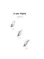
Cover. This is Cramer’s Rule for the system x + 2y = 6, 3x + y = 8. The size of the
first box is the determinant shown (the absolute value of the size is the area). The
size of the second box is x times that, and equals the size of the final box. Hence, x
is the final determinant divided by the first determinant.
Contents
Chapter One:
Linear Systems
I Solving Linear Systems . . . . . . . . . .
1 Gauss’ Method . . . . . . . . . . . . .
2 Describing the Solution Set . . . . . .
3 General = Particular + Homogeneous
II Linear Geometry of n-Space . . . . . . .
1 Vectors in Space . . . . . . . . . . . .
2 Length and Angle Measures∗ . . . . .
III Reduced Echelon Form . . . . . . . . . .
1 Gauss-Jordan Reduction . . . . . . . .
2 Row Equivalence . . . . . . . . . . . .
Topic: Computer Algebra Systems . . . . .
Topic: Input-Output Analysis . . . . . . . .
Topic: Accuracy of Computations . . . . . .
Topic: Analyzing Networks . . . . . . . . . .
Chapter Two:
Vector Spaces
I Definition of Vector Space . . . . . .
1 Definition and Examples . . . . . .
2 Subspaces and Spanning Sets . . .
II Linear Independence . . . . . . . . .
1 Definition and Examples . . . . . .
III Basis and Dimension . . . . . . . . .
1 Basis . . . . . . . . . . . . . . . . .
2 Dimension . . . . . . . . . . . . . .
3 Vector Spaces and Linear Systems
4 Combining Subspaces∗ . . . . . . .
Topic: Fields . . . . . . . . . . . . . . . .
Topic: Crystals . . . . . . . . . . . . . .
Topic: Voting Paradoxes . . . . . . . . .
Topic: Dimensional Analysis . . . . . . .
vii
.
.
.
.
.
.
.
.
.
.
.
.
.
.
.
.
.
.
.
.
.
.
.
.
.
.
.
.
.
.
.
.
.
.
.
.
.
.
.
.
.
.
.
.
.
.
.
.
.
.
.
.
.
.
.
.
.
.
.
.
.
.
.
.
.
.
.
.
.
.
.
.
.
.
.
.
.
.
.
.
.
.
.
.
.
.
.
.
.
.
.
.
.
.
.
.
.
.
.
.
.
.
.
.
.
.
.
.
.
.
.
.
.
.
.
.
.
.
.
.
.
.
.
.
.
.
.
.
.
.
.
.
.
.
.
.
.
.
.
.
.
.
.
.
.
.
.
.
.
.
.
.
.
.
.
.
.
.
.
.
.
.
.
.
.
.
.
.
.
.
.
.
.
.
.
.
.
.
.
.
.
.
.
.
.
.
.
.
.
.
.
.
.
.
.
.
.
.
.
.
.
.
.
.
.
.
.
.
.
.
.
.
.
.
.
.
.
.
.
.
.
.
.
.
.
.
.
.
.
.
.
.
.
.
.
.
.
.
.
.
.
.
.
.
.
.
.
.
.
.
.
.
.
.
.
.
.
.
.
.
.
.
.
.
.
.
.
.
.
.
.
.
.
.
.
.
.
.
.
.
.
.
.
.
.
.
.
.
.
.
.
.
.
.
.
.
.
.
.
.
.
.
.
.
.
.
.
.
.
.
.
.
.
.
.
.
.
.
.
.
.
.
.
.
.
.
.
.
.
.
.
.
.
.
.
.
.
.
.
.
.
.
.
.
.
.
.
.
.
.
.
.
.
.
.
.
.
.
.
.
.
.
.
.
.
.
.
.
.
.
.
.
.
.
.
.
.
.
.
.
.
.
.
.
.
.
.
.
.
.
.
.
.
.
.
.
.
.
.
.
.
.
.
.
.
.
1
1
2
11
20
32
32
38
46
46
52
62
64
68
72
.
.
.
.
.
.
.
.
.
.
.
.
.
.
79
80
80
91
102
102
113
113
119
124
131
141
143
147
152
Chapter Three: Maps Between Spaces
I Isomorphisms . . . . . . . . . . . . . . . .
1 Definition and Examples . . . . . . . . .
2 Dimension Characterizes Isomorphism .
II Homomorphisms . . . . . . . . . . . . . .
1 Definition . . . . . . . . . . . . . . . . .
2 Rangespace and Nullspace . . . . . . . .
III Computing Linear Maps . . . . . . . . . .
1 Representing Linear Maps with Matrices
2 Any Matrix Represents a Linear Map∗ .
IV Matrix Operations . . . . . . . . . . . . .
1 Sums and Scalar Products . . . . . . . .
2 Matrix Multiplication . . . . . . . . . .
3 Mechanics of Matrix Multiplication . . .
4 Inverses . . . . . . . . . . . . . . . . . .
V Change of Basis . . . . . . . . . . . . . . .
1 Changing Representations of Vectors . .
2 Changing Map Representations . . . . .
VI Projection . . . . . . . . . . . . . . . . . .
1 Orthogonal Projection Into a Line∗ . . .
2 Gram-Schmidt Orthogonalization∗ . . .
3 Projection Into a Subspace∗ . . . . . . .
Topic: Line of Best Fit . . . . . . . . . . . . .
Topic: Geometry of Linear Maps . . . . . . .
Topic: Markov Chains . . . . . . . . . . . . .
Topic: Orthonormal Matrices . . . . . . . . .
.
.
.
.
.
.
.
.
.
.
.
.
.
.
.
.
.
.
.
.
.
.
.
.
.
.
.
.
.
.
.
.
.
.
.
.
.
.
.
.
.
.
.
.
.
.
.
.
.
.
.
.
.
.
.
.
.
.
.
.
.
.
.
.
.
.
.
.
.
.
.
.
.
.
.
.
.
.
.
.
.
.
.
.
.
.
.
.
.
.
.
.
.
.
.
.
.
.
.
.
.
.
.
.
.
.
.
.
.
.
.
.
.
.
.
.
.
.
.
.
.
.
.
.
.
.
.
.
.
.
.
.
.
.
.
.
.
.
.
.
.
.
.
.
.
.
.
.
.
.
.
.
.
.
.
.
.
.
.
.
.
.
.
.
.
.
.
.
.
.
.
.
.
.
.
.
.
.
.
.
.
.
.
.
.
.
.
.
.
.
.
.
.
.
.
.
.
.
.
.
.
.
.
.
.
.
.
.
.
.
.
.
.
.
.
.
.
.
.
.
.
.
.
.
.
.
.
.
.
.
.
.
.
.
.
.
.
.
.
.
.
.
.
.
.
.
.
.
.
.
.
.
.
.
.
.
.
.
.
.
.
.
.
.
.
.
.
.
.
.
.
.
.
.
.
.
.
.
.
.
.
.
.
.
.
.
.
.
.
.
.
.
.
.
.
.
.
.
.
.
.
.
.
.
.
.
.
.
.
.
.
.
.
.
.
.
.
.
.
.
.
.
.
.
.
159
159
159
168
176
176
183
195
195
205
212
212
214
222
231
238
238
242
250
250
254
260
269
274
281
287
Chapter Four: Determinants
I Definition . . . . . . . . . . . . . . . .
1 Exploration∗ . . . . . . . . . . . . .
2 Properties of Determinants . . . . .
3 The Permutation Expansion . . . . .
4 Determinants Exist∗ . . . . . . . . .
II Geometry of Determinants . . . . . . .
1 Determinants as Size Functions . . .
III Other Formulas . . . . . . . . . . . . .
1 Laplace’s Expansion∗ . . . . . . . . .
Topic: Cramer’s Rule . . . . . . . . . . . .
Topic: Speed of Calculating Determinants
Topic: Projective Geometry . . . . . . . .
.
.
.
.
.
.
.
.
.
.
.
.
.
.
.
.
.
.
.
.
.
.
.
.
.
.
.
.
.
.
.
.
.
.
.
.
.
.
.
.
.
.
.
.
.
.
.
.
.
.
.
.
.
.
.
.
.
.
.
.
.
.
.
.
.
.
.
.
.
.
.
.
.
.
.
.
.
.
.
.
.
.
.
.
.
.
.
.
.
.
.
.
.
.
.
.
.
.
.
.
.
.
.
.
.
.
.
.
.
.
.
.
.
.
.
.
.
.
.
.
.
.
.
.
.
.
.
.
.
.
.
.
.
.
.
.
.
.
.
.
.
.
.
.
.
.
.
.
.
.
.
.
.
.
.
.
293
294
294
299
303
312
319
319
326
326
331
334
337
. . . . . . .
A Review∗
. . . . . . .
. . . . . . .
.
.
.
.
.
.
.
.
.
.
.
.
.
.
.
.
.
.
.
.
.
.
.
.
.
.
.
.
.
.
.
.
.
.
.
.
.
.
.
.
349
349
350
351
353
Chapter Five:
Similarity
I Complex Vector Spaces . . . . . . .
1 Factoring and Complex Numbers;
2 Complex Representations . . . .
II Similarity . . . . . . . . . . . . . .
viii
.
.
.
.
.
.
.
.
.
.
.
.
.
.
.
.
.
.
.
.
.
.
.
.
1 Definition and Examples . . . . . .
2 Diagonalizability . . . . . . . . . .
3 Eigenvalues and Eigenvectors . . .
III Nilpotence . . . . . . . . . . . . . . .
1 Self-Composition∗ . . . . . . . . .
2 Strings∗ . . . . . . . . . . . . . . .
IV Jordan Form . . . . . . . . . . . . . .
1 Polynomials of Maps and Matrices∗
2 Jordan Canonical Form∗ . . . . . .
Topic: Method of Powers . . . . . . . . .
Topic: Stable Populations . . . . . . . .
Topic: Linear Recurrences . . . . . . . .
Appendix
Propositions . . . . . . . . . .
Quantifiers . . . . . . . . . .
Techniques of Proof . . . . .
Sets, Functions, and Relations
∗
.
.
.
.
.
.
.
.
Note: starred subsections are optional.
ix
.
.
.
.
.
.
.
.
.
.
.
.
.
.
.
.
.
.
.
.
.
.
.
.
.
.
.
.
.
.
.
.
.
.
.
.
.
.
.
.
.
.
.
.
.
.
.
.
.
.
.
.
.
.
.
.
.
.
.
.
.
.
.
.
.
.
.
.
.
.
.
.
.
.
.
.
.
.
.
.
.
.
.
.
.
.
.
.
.
.
.
.
.
.
.
.
.
.
.
.
.
.
.
.
.
.
.
.
.
.
.
.
.
.
.
.
.
.
.
.
.
.
.
.
.
.
.
.
.
.
.
.
.
.
.
.
.
.
.
.
.
.
.
.
.
.
.
.
.
.
.
.
.
.
.
.
.
.
.
.
.
.
.
.
.
.
.
.
.
.
.
.
.
.
.
.
.
.
.
.
.
.
.
.
.
.
.
.
.
.
.
.
.
.
.
.
.
.
.
.
.
.
.
.
353
355
359
367
367
370
381
381
388
401
405
407
.
.
.
.
.
.
.
.
.
.
.
.
.
.
.
.
.
.
.
.
.
.
.
.
.
.
.
.
.
.
.
.
.
.
.
.
.
.
.
.
.
.
.
.
.
.
.
.
.
.
.
.
.
.
.
.
.
.
.
.
.
.
.
.
A-1
A-1
A-3
A-5
A-7
Chapter One
Linear Systems
I
Solving Linear Systems
Systems of linear equations are common in science and mathematics. These two
examples from high school science [Onan] give a sense of how they arise.
The first example is from Physics. Suppose that we are given three objects,
one with a mass known to be 2 kg, and are asked to find the unknown masses.
Suppose further that experimentation with a meter stick produces these two
balances.
40
h
50
c
25
50
c
2
15
2
h
25
Since the sum of moments on the left of each balance equals the sum of moments
on the right (the moment of an object is its mass times its distance from the
balance point), the two balances give this system of two equations.
40h + 15c = 100
25c = 50 + 50h
The second example of a linear system is from Chemistry. We can mix,
under controlled conditions, toluene C7 H8 and nitric acid HNO3 to produce
trinitrotoluene C7 H5 O6 N3 along with the byproduct water (conditions have to
be controlled very well, indeed — trinitrotoluene is better known as TNT). In
what proportion should those components be mixed? The number of atoms of
each element present before the reaction
x C7 H8 + y HNO3
−→
z C7 H5 O6 N3 + w H2 O
must equal the number present afterward. Applying that principle to the ele1
2
Chapter One. Linear Systems
ments C, H, N, and O in turn gives this system.
7x = 7z
8x + 1y = 5z + 2w
1y = 3z
3y = 6z + 1w
To finish each of these examples requires solving a system of equations. In
each, the equations involve only the first power of the variables. This chapter
shows how to solve any such system.
I.1 Gauss’ Method
1.1 Definition A linear equation in variables x1 , x2 , . . . , xn has the form
a1 x1 + a2 x2 + a3 x3 + · · · + an xn = d
where the numbers a1 , . . . , an ∈ R are the equation’s coefficients and d ∈ R
is the constant. An n-tuple (s1 , s2 , . . . , sn ) ∈ Rn is a solution of, or satisfies,
that equation if substituting the numbers s1 , . . . , sn for the variables gives a
true statement: a1 s1 + a2 s2 + . . . + an sn = d.
A system of linear equations
a1,1 x1 + a1,2 x2 + · · · + a1,n xn = d1
a2,1 x1 + a2,2 x2 + · · · + a2,n xn = d2
..
.
am,1 x1 + am,2 x2 + · · · + am,n xn = dm
has the solution (s1 , s2 , . . . , sn ) if that n-tuple is a solution of all of the equations in the system.
1.2 Example The ordered pair (−1, 5) is a solution of this system.
3x1 + 2x2 = 7
−x1 + x2 = 6
In contrast, (5, −1) is not a solution.
Finding the set of all solutions is solving the system. No guesswork or good
fortune is needed to solve a linear system. There is an algorithm that always
works. The next example introduces that algorithm, called Gauss’ method. It
transforms the system, step by step, into one with a form that is easily solved.
Section I. Solving Linear Systems
3
1.3 Example To solve this system
3x3 = 9
x1 + 5x2 − 2x3 = 2
1
=3
3 x1 + 2x2
we repeatedly transform it until it is in a form that is easy to solve.
swap row 1 with row 3
−→
multiply row 1 by 3
−→
add −1 times row 1 to row 2
−→
1
3 x1
x1
+ 2x2
=3
+ 5x2 − 2x3 = 2
3x3 = 9
x1 + 6x2
=9
x1 + 5x2 − 2x3 = 2
3x3 = 9
x1 + 6x2
= 9
−x2 − 2x3 = −7
3x3 = 9
The third step is the only nontrivial one. We’ve mentally multiplied both sides
of the first row by −1, mentally added that to the old second row, and written
the result in as the new second row.
Now we can find the value of each variable. The bottom equation shows
that x3 = 3. Substituting 3 for x3 in the middle equation shows that x2 = 1.
Substituting those two into the top equation gives that x1 = 3 and so the system
has a unique solution: the solution set is { (3, 1, 3) }.
Most of this subsection and the next one consists of examples of solving
linear systems by Gauss’ method. We will use it throughout this book. It is
fast and easy. But, before we get to those examples, we will first show that
this method is also safe in that it never loses solutions or picks up extraneous
solutions.
1.4 Theorem (Gauss’ method) If a linear system is changed to another
by one of these operations
(1) an equation is swapped with another
(2) an equation has both sides multiplied by a nonzero constant
(3) an equation is replaced by the sum of itself and a multiple of another
then the two systems have the same set of solutions.
Each of those three operations has a restriction. Multiplying a row by 0 is
not allowed because obviously that can change the solution set of the system.
Similarly, adding a multiple of a row to itself is not allowed because adding −1
times the row to itself has the effect of multiplying the row by 0. Finally, swapping a row with itself is disallowed to make some results in the fourth chapter
easier to state and remember (and besides, self-swapping doesn’t accomplish
anything).
4
Chapter One. Linear Systems
Proof. We will cover the equation swap operation here and save the other two
cases for Exercise 29.
Consider this swap of row i with row j.
a1,1 x1 + a1,2 x2 + · · · a1,n xn = d1
a1,1 x1 + a1,2 x2 + · · ·
..
.
aj,1 x1 + aj,2 x2 + · · ·
ai,1 x1 + ai,2 x2 + · · · ai,n xn = di
..
−→
.
ai,1 x1 + ai,2 x2 + · · ·
aj,1 x1 + aj,2 x2 + · · · aj,n xn = dj
..
.
am,1 x1 + am,2 x2 + · · · am,n xn = dm
am,1 x1 + am,2 x2 + · · ·
a1,n xn = d1
..
.
aj,n xn = dj
..
.
ai,n xn = di
..
.
am,n xn = dm
The n-tuple (s1 , . . . , sn ) satisfies the system before the swap if and only if
substituting the values, the s’s, for the variables, the x’s, gives true statements:
a1,1 s1 +a1,2 s2 +· · ·+a1,n sn = d1 and . . . ai,1 s1 +ai,2 s2 +· · ·+ai,n sn = di and . . .
aj,1 s1 + aj,2 s2 + · · · + aj,n sn = dj and . . . am,1 s1 + am,2 s2 + · · · + am,n sn = dm .
In a requirement consisting of statements and-ed together we can rearrange
the order of the statements, so that this requirement is met if and only if a1,1 s1 +
a1,2 s2 + · · · + a1,n sn = d1 and . . . aj,1 s1 + aj,2 s2 + · · · + aj,n sn = dj and . . .
ai,1 s1 + ai,2 s2 + · · · + ai,n sn = di and . . . am,1 s1 + am,2 s2 + · · · + am,n sn = dm .
This is exactly the requirement that (s1 , . . . , sn ) solves the system after the row
swap.
QED
1.5 Definition The three operations from Theorem 1.4 are the elementary
reduction operations, or row operations, or Gaussian operations. They are
swapping, multiplying by a scalar or rescaling, and pivoting.
When writing out the calculations, we will abbreviate ‘row i’ by ‘ρi ’. For
instance, we will denote a pivot operation by kρi + ρj , with the row that is
changed written second. We will also, to save writing, often list pivot steps
together when they use the same ρi .
1.6 Example A typical use of Gauss’ method is to solve this system.
x+ y
=0
2x − y + 3z = 3
x − 2y − z = 3
The first transformation of the system involves using the first row to eliminate
the x in the second row and the x in the third. To get rid of the second row’s
2x, we multiply the entire first row by −2, add that to the second row, and
write the result in as the new second row. To get rid of the third row’s x, we
multiply the first row by −1, add that to the third row, and write the result in
as the new third row.
−2ρ1 +ρ2
−→
−ρ1 +ρ3
x+
y
=0
−3y + 3z = 3
−3y − z = 3
Section I. Solving Linear Systems
5
(Note that the two ρ1 steps −2ρ1 + ρ2 and −ρ1 + ρ3 are written as one operation.) In this second system, the last two equations involve only two unknowns.
To finish we transform the second system into a third system, where the last
equation involves only one unknown. This transformation uses the second row
to eliminate y from the third row.
−ρ2 +ρ3
x+
−→
y
−3y +
=0
3z = 3
−4z = 0
Now we are set up for the solution. The third row shows that z = 0. Substitute
that back into the second row to get y = −1, and then substitute back into the
first row to get x = 1.
1.7 Example For the Physics problem from the start of this chapter, Gauss’
method gives this.
40h + 15c = 100
−50h + 25c = 50
40h +
5/4ρ1 +ρ2
−→
15c = 100
(175/4)c = 175
So c = 4, and back-substitution gives that h = 1. (The Chemistry problem is
solved later.)
1.8 Example The reduction
x+ y+ z=9
2x + 4y − 3z = 1
3x + 6y − 5z = 0
−2ρ1 +ρ2
−→
−3ρ1 +ρ3
−(3/2)ρ2 +ρ3
−→
x+ y+ z= 9
2y − 5z = −17
3y − 8z = −27
x+ y+
2y −
z=
9
5z =
−17
−(1/2)z = −(3/2)
shows that z = 3, y = −1, and x = 7.
As these examples illustrate, Gauss’ method uses the elementary reduction
operations to set up back-substitution.
1.9 Definition In each row, the first variable with a nonzero coefficient is the
row’s leading variable. A system is in echelon form if each leading variable is
to the right of the leading variable in the row above it (except for the leading
variable in the first row).
1.10 Example The only operation needed in the examples above is pivoting.
Here is a linear system that requires the operation of swapping equations. After
the first pivot
x− y
=0
2x − 2y + z + 2w = 4
y
+ w=0
2z + w = 5
x−y
−2ρ1 +ρ2
−→
=0
z + 2w = 4
y
+ w=0
2z + w = 5
6
Chapter One. Linear Systems
the second equation has no leading y. To get one, we look lower down in the
system for a row that has a leading y and swap it in.
ρ2 ↔ρ3
−→
x−y
y
=0
+ w=0
z + 2w = 4
2z + w = 5
(Had there been more than one row below the second with a leading y then we
could have swapped in any one.) The rest of Gauss’ method goes as before.
−2ρ3 +ρ4
−→
x−y
y
+
z+
= 0
w= 0
2w = 4
−3w = −3
Back-substitution gives w = 1, z = 2 , y = −1, and x = −1.
Strictly speaking, the operation of rescaling rows is not needed to solve linear
systems. We have included it because we will use it later in this chapter as part
of a variation on Gauss’ method, the Gauss-Jordan method.
All of the systems seen so far have the same number of equations as unknowns. All of them have a solution, and for all of them there is only one
solution. We finish this subsection by seeing for contrast some other things that
can happen.
1.11 Example Linear systems need not have the same number of equations
as unknowns. This system
x + 3y = 1
2x + y = −3
2x + 2y = −2
has more equations than variables. Gauss’ method helps us understand this
system also, since this
−2ρ1 +ρ2
−→
−2ρ1 +ρ3
x + 3y = 1
−5y = −5
−4y = −4
shows that one of the equations is redundant. Echelon form
−(4/5)ρ2 +ρ3
−→
x + 3y = 1
−5y = −5
0= 0
gives y = 1 and x = −2. The ‘0 = 0’ is derived from the redundancy.
That example’s system has more equations than variables. Gauss’ method
is also useful on systems with more variables than equations. Many examples
are in the next subsection.
Section I. Solving Linear Systems
7
Another way that linear systems can differ from the examples shown earlier
is that some linear systems do not have a unique solution. This can happen in
two ways.
The first is that it can fail to have any solution at all.
1.12 Example Contrast the system in the last example with this one.
x + 3y = 1
2x + y = −3
2x + 2y = 0
−2ρ1 +ρ2
x+
−→
−2ρ1 +ρ3
3y = 1
−5y = −5
−4y = −2
Here the system is inconsistent: no pair of numbers satisfies all of the equations
simultaneously. Echelon form makes this inconsistency obvious.
−(4/5)ρ2 +ρ3
−→
x + 3y = 1
−5y = −5
0= 2
The solution set is empty.
1.13 Example The prior system has more equations than unknowns, but that
is not what causes the inconsistency — Example 1.11 has more equations than
unknowns and yet is consistent. Nor is having more equations than unknowns
necessary for inconsistency, as is illustrated by this inconsistent system with the
same number of equations as unknowns.
x + 2y = 8
2x + 4y = 8
−2ρ1 +ρ2
−→
x + 2y = 8
0 = −8
The other way that a linear system can fail to have a unique solution is to
have many solutions.
1.14 Example In this system
x+ y=4
2x + 2y = 8
any pair of numbers satisfying the
¯ first equation automatically satisfies the second. The solution set {(x, y) ¯ x + y = 4} is infinite; some of its members
are (0, 4), (−1, 5), and (2.5, 1.5). The result of applying Gauss’ method here
contrasts with the prior example because we do not get a contradictory equation.
−2ρ1 +ρ2
−→
x+y=4
0=0
Don’t be fooled by the ‘0 = 0’ equation in that example. It is not the signal
that a system has many solutions.
8
Chapter One. Linear Systems
1.15 Example The absence of a ‘0 = 0’ does not keep a system from having
many different solutions. This system is in echelon form
x+y+z=0
y+z=0
has no ‘0 = 0’, and yet has infinitely many solutions. (For instance, each of
these is a solution: (0, 1, −1), (0, 1/2, −1/2), (0, 0, 0), and (0, −π, π). There are
infinitely many solutions because any triple whose first component is 0 and
whose second component is the negative of the third is a solution.)
Nor does the presence of a ‘0 = 0’ mean that the system must have many
solutions. Example 1.11 shows that. So does this system, which does not have
many solutions — in fact it has none — despite that when it is brought to echelon
form it has a ‘0 = 0’ row.
2x
− 2z = 6
y+ z=1
2x + y − z = 7
3y + 3z = 0
2x
− 2z = 6
y+ z=1
y+ z=1
3y + 3z = 0
2x
− 2z = 6
y+ z= 1
0= 0
0 = −3
−ρ1 +ρ3
−→
−ρ2 +ρ3
−→
−3ρ2 +ρ4
We will finish this subsection with a summary of what we’ve seen so far
about Gauss’ method.
Gauss’ method uses the three row operations to set a system up for back
substitution. If any step shows a contradictory equation then we can stop
with the conclusion that the system has no solutions. If we reach echelon form
without a contradictory equation, and each variable is a leading variable in its
row, then the system has a unique solution and we find it by back substitution.
Finally, if we reach echelon form without a contradictory equation, and there is
not a unique solution (at least one variable is not a leading variable) then the
system has many solutions.
The next subsection deals with the third case — we will see how to describe
the solution set of a system with many solutions.
Exercises
X 1.16 Use Gauss’ method to find the unique solution for each system.
x
−z=0
2x + 3y = 13
=1
(a)
(b) 3x + y
x − y = −1
−x + y + z = 4
X 1.17 Use Gauss’ method to solve each system or conclude ‘many solutions’ or ‘no
solutions’.
Section I. Solving Linear Systems
9
(a) 2x + 2y = 5
(b) −x + y = 1
(c) x − 3y + z = 1
x − 4y = 0
x+y=2
x + y + 2z = 14
(d) −x − y = 1
(e)
4y + z = 20
(f ) 2x
+ z+w= 5
−3x − 3y = 2
2x − 2y + z = 0
y
− w = −1
x
+z= 5
3x
− z−w= 0
x + y − z = 10
4x + y + 2z + w = 9
X 1.18 There are methods for solving linear systems other than Gauss’ method. One
often taught in high school is to solve one of the equations for a variable, then
substitute the resulting expression into other equations. That step is repeated
until there is an equation with only one variable. From that, the first number in
the solution is derived, and then back-substitution can be done. This method both
takes longer than Gauss’ method, since it involves more arithmetic operations and
is more likely to lead to errors. To illustrate how it can lead to wrong conclusions,
we will use the system
x + 3y = 1
2x + y = −3
2x + 2y = 0
from Example 1.12.
(a) Solve the first equation for x and substitute that expression into the second
equation. Find the resulting y.
(b) Again solve the first equation for x, but this time substitute that expression
into the third equation. Find this y.
What extra step must a user of this method take to avoid erroneously concluding
a system has a solution?
X 1.19 For which values of k are there no solutions, many solutions, or a unique
solution to this system?
x− y=1
3x − 3y = k
X 1.20 This system is not linear, in some sense,
2 sin α − cos β + 3 tan γ = 3
4 sin α + 2 cos β − 2 tan γ = 10
6 sin α − 3 cos β + tan γ = 9
and yet we can nonetheless apply Gauss’ method. Do so. Does the system have a
solution?
X 1.21 What conditions must the constants, the b’s, satisfy so that each of these
systems has a solution? Hint. Apply Gauss’ method and see what happens to the
right side. [Anton]
(a) x − 3y = b1
(b) x1 + 2x2 + 3x3 = b1
3x + y = b2
2x1 + 5x2 + 3x3 = b2
x + 7y = b3
x1
+ 8x3 = b3
2x + 4y = b4
1.22 True or false: a system with more unknowns than equations has at least one
solution. (As always, to say ‘true’ you must prove it, while to say ‘false’ you must
produce a counterexample.)
1.23 Must any Chemistry problem like the one that starts this subsection — a balance the reaction problem — have infinitely many solutions?
X 1.24 Find the coefficients a, b, and c so that the graph of f (x) = ax2 + bx + c passes
through the points (1, 2), (−1, 6), and (2, 3).
10
Chapter One. Linear Systems
1.25 Gauss’ method works by combining the equations in a system to make new
equations.
(a) Can the equation 3x−2y = 5 be derived, by a sequence of Gaussian reduction
steps, from the equations in this system?
x+y=1
4x − y = 6
(b) Can the equation 5x−3y = 2 be derived, by a sequence of Gaussian reduction
steps, from the equations in this system?
2x + 2y = 5
3x + y = 4
(c) Can the equation 6x − 9y + 5z = −2 be derived, by a sequence of Gaussian
reduction steps, from the equations in the system?
2x + y − z = 4
6x − 3y + z = 5
1.26 Prove that, where a, b, . . . , e are real numbers and a 6= 0, if
ax + by = c
has the same solution set as
ax + dy = e
then they are the same equation. What if a = 0?
X 1.27 Show that if ad − bc 6= 0 then
ax + by = j
cx + dy = k
has a unique solution.
X 1.28 In the system
ax + by = c
dx + ey = f
each of the equations describes a line in the xy-plane. By geometrical reasoning,
show that there are three possibilities: there is a unique solution, there is no
solution, and there are infinitely many solutions.
1.29 Finish the proof of Theorem 1.4.
1.30 Is there a two-unknowns linear system whose solution set is all of R2 ?
X 1.31 Are any of the operations used in Gauss’ method redundant? That is, can
any of the operations be synthesized from the others?
1.32 Prove that each operation of Gauss’ method is reversible. That is, show that if
two systems are related by a row operation S1 → S2 then there is a row operation
to go back S2 → S1 .
? 1.33 A box holding pennies, nickels and dimes contains thirteen coins with a total
value of 83 cents. How many coins of each type are in the box? [Anton]
? 1.34 Four positive integers are given. Select any three of the integers, find their
arithmetic average, and add this result to the fourth integer. Thus the numbers
29, 23, 21, and 17 are obtained. One of the original integers is:
Section I. Solving Linear Systems
11
(a) 19
(b) 21
(c) 23
(d) 29
(e) 17
[Con. Prob. 1955]
? X 1.35 Laugh at this: AHAHA + TEHE = TEHAW. It resulted from substituting
a code letter for each digit of a simple example in addition, and it is required to
identify the letters and prove the solution unique. [Am. Math. Mon., Jan. 1935]
? 1.36 The Wohascum County Board of Commissioners, which has 20 members, recently had to elect a President. There were three candidates (A, B, and C); on
each ballot the three candidates were to be listed in order of preference, with no
abstentions. It was found that 11 members, a majority, preferred A over B (thus
the other 9 preferred B over A). Similarly, it was found that 12 members preferred
C over A. Given these results, it was suggested that B should withdraw, to enable
a runoff election between A and C. However, B protested, and it was then found
that 14 members preferred B over C! The Board has not yet recovered from the resulting confusion. Given that every possible order of A, B, C appeared on at least
one ballot, how many members voted for B as their first choice? [Wohascum no. 2]
? 1.37 “This system of n linear equations with n unknowns,” said the Great Mathematician, “has a curious property.”
“Good heavens!” said the Poor Nut, “What is it?”
“Note,” said the Great Mathematician, “that the constants are in arithmetic
progression.”
“It’s all so clear when you explain it!” said the Poor Nut. “Do you mean like
6x + 9y = 12 and 15x + 18y = 21?”
“Quite so,” said the Great Mathematician, pulling out his bassoon. “Indeed,
the system has a unique solution. Can you find it?”
“Good heavens!” cried the Poor Nut, “I am baffled.”
Are you? [Am. Math. Mon., Jan. 1963]
I.2 Describing the Solution Set
A linear system with a unique solution has a solution set with one element. A
linear system with no solution has a solution set that is empty. In these cases
the solution set is easy to describe. Solution sets are a challenge to describe
only when they contain many elements.
2.1 Example This system has many solutions because in echelon form
2x
+z=3
x−y−z=1
3x − y
=4
−(1/2)ρ1 +ρ2
2x
+
z=
3
−y − (3/2)z = −1/2
−y − (3/2)z = −1/2
2x
+
z=
3
−y − (3/2)z = −1/2
0=
0
−→
−(3/2)ρ1 +ρ3
−ρ2 +ρ3
−→
not all of the variables are leading variables. The Gauss’ method theorem
showed that a triple satisfies the¯ first system if and only if it satisfies the third.
Thus, the solution set {(x, y, z) ¯ 2x + z = 3 and x − y − z = 1 and 3x − y = 4}
12
Chapter One. Linear Systems
¯
can also be described as {(x, y, z) ¯ 2x + z = 3 and −y − 3z/2 = −1/2}. However, this second description is not much of an improvement. It has two equations instead of three, but it still involves some hard-to-understand interaction
among the variables.
To get a description that is free of any such interaction, we take the variable that does not lead any equation, z, and use it to describe the variables
that do lead, x and y. The second equation gives y = (1/2) − (3/2)z and
the first equation gives x = (3/2) − (1/2)z. Thus, the solution
set can be de¯
scribed as {(x, y, z) = ((3/2) − (1/2)z, (1/2) − (3/2)z, z) ¯ z ∈ R}. For instance,
(1/2, −5/2, 2) is a solution because taking z = 2 gives a first component of 1/2
and a second component of −5/2.
The advantage of this description over the ones above is that the only variable
appearing, z, is unrestricted — it can be any real number.
2.2 Definition The non-leading variables in an echelon-form linear system
are free variables.
In the echelon form system derived in the above example, x and y are leading
variables and z is free.
2.3 Example A linear system can end with more than one variable free. This
row reduction
x+ y+ z− w= 1
y − z + w = −1
3x
+ 6z − 6w = 6
−y + z − w = 1
x+
−3ρ1 +ρ3
−→
3ρ2 +ρ3
−→
ρ2 +ρ4
y+ z− w= 1
y − z + w = −1
−3y + 3z − 3w = 3
−y + z − w = 1
x+y+z−w= 1
y − z + w = −1
0= 0
0= 0
ends with x and y leading, and with both z and w free. To get the description
that we prefer we will start at the bottom. We first express y in terms of
the free variables z and w with y = −1 + z − w. Next, moving up to the
top equation, substituting for y in the first equation x + (−1 + z − w) + z −
w = 1 and solving for x yields¯ x = 2 − 2z + 2w. Thus, the solution set is
{2 − 2z + 2w, −1 + z − w, z, w) ¯ z, w ∈ R}.
We prefer this description because the only variables that appear, z and w,
are unrestricted. This makes the job of deciding which four-tuples are system
solutions into an easy one. For instance, taking z = 1 and w = 2 gives the
solution (4, −2, 1, 2). In contrast, (3, −2, 1, 2) is not a solution, since the first
component of any solution must be 2 minus twice the third component plus
twice the fourth.
Section I. Solving Linear Systems
13
2.4 Example After this reduction
2x − 2y
=0
z + 3w = 2
3x − 3y
=0
x − y + 2z + 6w = 4
2x − 2y
=0
z + 3w = 2
0=0
2z + 6w = 4
2x − 2y
=0
z + 3w = 2
0=0
0=0
−(3/2)ρ1 +ρ3
−→
−(1/2)ρ1 +ρ4
−2ρ2 +ρ4
−→
¯
x and z lead, y and w are free. The solution set is {(y, y, 2 − 3w, w) ¯ y, w ∈ R}.
For instance, (1, 1, 2, 0) satisfies the system — take y = 1 and w = 0. The fourtuple (1, 0, 5, 4) is not a solution since its first coordinate does not equal its
second.
We refer to a variable used to describe a family of solutions as a parameter
and we say that the set above is paramatrized with y and w. (The terms
‘parameter’ and ‘free variable’ do not mean the same thing. Above, y and w
are free because in the echelon form system they do not lead any row. They
are parameters because they are used in the solution set description. We could
have instead paramatrized with y and z by rewriting the second equation as
w = 2/3 − (1/3)z. In that case, the free variables are still y and w, but the
parameters are y and z. Notice that we could not have paramatrized with x and
y, so there is sometimes a restriction on the choice of parameters. The terms
‘parameter’ and ‘free’ are related because, as we shall show later in this chapter,
the solution set of a system can always be paramatrized with the free variables.
Consequenlty, we shall paramatrize all of our descriptions in this way.)
2.5 Example This is another system with infinitely many solutions.
x + 2y
=1
2x
+z
=2
3x + 2y + z − w = 4
−2ρ1 +ρ2
x+
2y
=1
−4y + z
=0
−4y + z − w = 1
x+
2y
−4y + z
−→
−3ρ1 +ρ3
−ρ2 +ρ3
−→
=1
=0
−w = 1
The leading variables are x, y, and w. The variable z is free. (Notice here that,
although there are infinitely many solutions, the value of one of the variables is
fixed — w = −1.) Write w in terms of z with w = −1 + 0z. Then y = (1/4)z.
To express x in terms of z, substitute for y into the first ¯equation to get x =
1 − (1/2)z. The solution set is {(1 − (1/2)z, (1/4)z, z, −1) ¯ z ∈ R}.
We finish this subsection by developing the notation for linear systems and
their solution sets that we shall use in the rest of this book.
2.6 Definition An m × n matrix is a rectangular array of numbers with
m rows and n columns. Each number in the matrix is an entry,
14
Chapter One. Linear Systems
Matrices are usually named by upper case roman letters, e.g. A. Each entry is
denoted by the corresponding lower-case letter, e.g. ai,j is the number in row i
and column j of the array. For instance,
µ
1 2.2 5
A=
3 4 −7
has two rows and three columns, and so is a 2 × 3 matrix. (Read that “twoby-three”; the number of rows is always stated first.) The entry in the second
row and first column is a2,1 = 3. Note that the order of the subscripts matters:
a1,2 6= a2,1 since a1,2 = 2.2. (The parentheses around the array are a typographic device so that when two matrices are side by side we can tell where one
ends and the other starts.)
2.7 Example We can abbreviate this linear system
x1 + 2x2
=4
x2 − x3 = 0
x1
+ 2x3 = 4
with this matrix.
1 2
0 1
1 0
0
−1
2
4
0
4
The vertical bar just reminds a reader of the difference between the coefficients
on the systems’s left hand side and the constants on the right. When a bar
is used to divide a matrix into parts, we call it an augmented matrix. In this
notation, Gauss’ method goes this way.
1 2 0 4
1 2
0 4
1 2 0 4
1 +ρ3
2 +ρ3
0 1 −1 0 −ρ−→
0 1 −1 0 2ρ−→
0 1 −1 0
1 0 2 4
0 −2 2 0
0 0 0 0
The second row stands for y − z¯= 0 and the first row stands for x + 2y = 4 so
the solution set is {(4 − 2z, z, z) ¯ z ∈ R}. One advantage of the new notation is
that the clerical load of Gauss’ method — the copying of variables, the writing
of +’s and =’s, etc. — is lighter.
We will also use the array notation to clarify the descriptions
of solution
¯
sets. A description like {(2 − 2z + 2w, −1 + z − w, z, w) ¯ z, w ∈ R} from Example 2.3 is hard to read. We will rewrite it to group all the constants together,
all the coefficients of z together, and all the coefficients of w together. We will
write them vertically, in one-column wide matrices.
2
−2
2
−1 1
−1
¯
¯
{
0 + 1 · z + 0 · w z, w ∈ R}
0
0
1
Section I. Solving Linear Systems
15
For instance, the top line says that x = 2 − 2z + 2w. The next section gives a
geometric interpretation that will help us picture the solution sets when they
are written in this way.
2.8 Definition A vector (or column vector ) is a matrix with a single column.
A matrix with a single row is a row vector . The entries of a vector are its
components.
Vectors are an exception to the convention of representing matrices with
capital roman letters. We use lower-case roman or greek letters overlined with
~ . . . (boldface is also common: a or α). For instance,
an arrow: ~a, ~b, . . . or α
~ , β,
this is a column vector with a third component of 7.
1
~v = 3
7
2.9 Definition The linear equation a1 x1 + a2 x2 + · · · + an xn = d with
unknowns x1 , . . . , xn is satisfied by
s1
..
~s = .
sn
if a1 s1 + a2 s2 + · · · + an sn = d. A vector satisfies a linear system if it satisfies
each equation in the system.
The style of description of solution sets that we use involves adding the
vectors, and also multiplying them by real numbers, such as the z and w. We
need to define these operations.
2.10 Definition The vector sum of ~u and ~v is this.
u1
v1
u1 + v1
..
~u + ~v = ... + ... =
.
un
vn
u n + vn
In general, two matrices with the same number of rows and the same number
of columns add in this way, entry-by-entry.
2.11 Definition The scalar multiplication of the real number r and the vector
~v is this.
v1
rv1
r · ~v = r · ... = ...
vn
rvn
In general, any matrix is multiplied by a real number in this entry-by-entry
way.
16
Chapter One. Linear Systems
Scalar multiplication can be written in either order: r · ~v or ~v · r, or without
the ‘·’ symbol: r~v . (Do not refer to scalar multiplication as ‘scalar product’
because that name is used for a different operation.)
2.12 Example
2
3
2+3
5
3 + −1 = 3 − 1 = 2
1
4
1+4
5
1
7
4 28
7·
−1 = −7
−3
−21
Notice that the definitions of vector addition and scalar multiplication agree
where they overlap, for instance, ~v + ~v = 2~v .
With the notation defined, we can now solve systems in the way that we will
use throughout this book.
2.13 Example This system
2x + y
− w
=4
y
+ w+u=4
x
− z + 2w
=0
reduces in
2 1
0 1
1 0
this way.
0
0
−1
−1 0
1 1
2 0
4
4
0
−(1/2)ρ1 +ρ3
−→
(1/2)ρ2 +ρ3
−→
2
1
0
1
0 −1/2
2 1 0
0 1 0
0 0 −1
0 −1 0
0
1
1
−1 5/2 0
−1 0
1
1
3 1/2
4
4
−2
4
4
0
¯
The solution set is {(w + (1/2)u, 4 − w − u, 3w + (1/2)u, w, u) ¯ w, u ∈ R}. We
write that in vector form.
x
0
1
1/2
y 4 −1
−1
¯
¯
{ z = 0 + 3 w +
1/2 u w, u ∈ R}
w 0 1
0
u
0
0
1
Note again how well vector notation sets off the coefficients of each parameter.
For instance, the third row of the vector form shows plainly that if u is held
fixed then z increases three times as fast as w.
That format also shows plainly that there are infinitely many solutions. For
example, we can fix u as 0, let w range over the real numbers, and consider the
first component x. We get infinitely many first components and hence infinitely
many solutions.
Section I. Solving Linear Systems
17
Another thing shown plainly is that setting both w and u to zero gives that
this
x
0
y 4
z = 0
w 0
u
0
is a particular solution of the linear system.
2.14 Example In the same way, this system
x− y+ z=1
3x
+ z=3
5x − 2y + 3z = 5
reduces
1 −1 1
3 0 1
5 −2 3
1
1 −1
−3ρ1 +ρ2
3 −→ 0 3
−5ρ1 +ρ3
5
0 3
1
−2
−2
1 −1
1
−ρ2 +ρ3
0 −→ 0 3
0
0 0
1
−2
0
1
0
0
to a one-parameter solution set.
1
−1/3
¯
{0 + 2/3 z ¯ z ∈ R}
0
1
Before the exercises, we pause to point out some things that we have yet to
do.
The first two subsections have been on the mechanics of Gauss’ method.
Except for one result, Theorem 1.4 — without which developing the method
doesn’t make sense since it says that the method gives the right answers — we
have not stopped to consider any of the interesting questions that arise.
For example, can we always describe solution sets as above, with a particular
solution vector added to an unrestricted linear combination of some other vectors? The solution sets we described with unrestricted parameters were easily
seen to have infinitely many solutions so an answer to this question could tell
us something about the size of solution sets. An answer to that question could
also help us picture the solution sets, in R2 , or in R3 , etc.
Many questions arise from the observation that Gauss’ method can be done
in more than one way (for instance, when swapping rows, we may have a choice
of which row to swap with). Theorem 1.4 says that we must get the same
solution set no matter how we proceed, but if we do Gauss’ method in two
different ways must we get the same number of free variables both times, so
that any two solution set descriptions have the same number of parameters?
Must those be the same variables (e.g., is it impossible to solve a problem one
way and get y and w free or solve it another way and get y and z free)?
18
Chapter One. Linear Systems
In the rest of this chapter we answer these questions. The answer to each
is ‘yes’. The first question is answered in the last subsection of this section. In
the second section we give a geometric description of solution sets. In the final
section of this chapter we tackle the last set of questions. Consequently, by the
end of the first chapter we will not only have a solid grounding in the practice
of Gauss’ method, we will also have a solid grounding in the theory. We will be
sure of what can and cannot happen in a reduction.
Exercises
X 2.15 Find the indicated entry of the matrix, if it is defined.
µ
A=
1
2
3
−1
1
4
(a) a2,1
(b) a1,2
(c) a2,2
(d) a3,1
X 2.16 Give the size of each matrix.
Ã
!
µ
µ
1
1
1 0 4
5 10
1
(a)
(b) −1
(c)
2 1 5
10 5
3
−1
X 2.17 Do the indicated vector operation, if it is defined.
à ! à !
à ! à !
µ 
µ 
µ 
3
3
2
1
3
4
2
+9
(a) 1 + 0
(b) 5
(c) 5 − 1
(d) 7
5
−1
1
4
1
1
1
!
!
!
Ã
Ã
!
Ã
Ã
µ 
1
1
2
3
1
+ 2
(e)
(f ) 6 1 − 4 0 + 2 1
2
5
3
3
1
X 2.18 Solve each system using matrix notation. Express the solution using vectors.
(a) 3x + 6y = 18
(b) x + y = 1
(c) x1
+ x3 = 4
x + 2y = 6
x − y = −1
x1 − x2 + 2x3 = 5
4x1 − x2 + 5x3 = 17
(d) 2a + b − c = 2
(e) x + 2y − z
=3
(f ) x
+z+w=4
2a
+c=3
2x + y
+w=4
2x + y
−w=2
a−b
=0
x− y+z+w=1
3x + y + z
=7
X 2.19 Solve each system using matrix notation. Give each solution set in vector
notation.
(a) 2x + y − z = 1
(b) x
− z
=1
(c) x − y + z
=0
4x − y
=3
y + 2z − w = 3
y
+w=0
x + 2y + 3z − w = 7
3x − 2y + 3z + w = 0
−y
−w=0
(d) a + 2b + 3c + d − e = 1
3a − b + c + d + e = 3
X 2.20 The vector is in the set. What value of the parameters produces that vector? µ ¶ µ 
¯
5
1
(a)
,{
k ¯ k ∈ R}
−5
−1
à ! à !
à !
−1
−2
3
¯
2 , { 1 i + 0 j ¯ i, j ∈ R}
(b)
1
0
1
Section I. Solving Linear Systems
Ã
!
à !
19
à !
0
1
2
¯
(c) −4 , { 1 m + 0 n ¯ m, n ∈ R}
2
0
1
2.21 Decide
is in the set.
µ ¶if the
µ vector
¯
3
−6
(a)
,{
k ¯ k ∈ R}
−1
2
µ 
X
X
X
X
?
µ
¯
5
5
(b)
,{
j ¯ j ∈ R}
4
−4
à ! à ! à !
2
0
1
¯
1 ,{ 3
(c)
+ −1 r ¯ r ∈ R}
−1
−7
3
à ! à !
à !
1
2
−3
¯
(d) 0 , { 0 j + −1 k ¯ j, k ∈ R}
1
1
1
2.22 Paramatrize the solution set of this one-equation system.
x1 + x2 + · · · + xn = 0
2.23 (a) Apply Gauss’ method to the left-hand side to solve
x + 2y
− w=a
2x
+z
=b
x+ y
+ 2w = c
for x, y, z, and w, in terms of the constants a, b, and c.
(b) Use your answer from the prior part to solve this.
x + 2y
− w= 3
2x
+z
= 1
x+ y
+ 2w = −2
2.24 Why is the comma needed in the notation ‘ai,j ’ for matrix entries?
2.25 Give the 4×4 matrix whose i, j-th entry is
(a) i + j;
(b) −1 to the i + j power.
2.26 For any matrix A, the transpose of A, written Atrans , is the matrix whose
columns are the rows of A. Find the transpose of each of these.
à !
µ
µ
µ
1
1 2 3
2 −3
5 10
(a)
(b)
(c)
(d) 1
4 5 6
1
1
10 5
0
2
2.27 (a) Describe all functions f (x) = ax + bx + c such that f (1) = 2 and
f (−1) = 6.
(b) Describe all functions f (x) = ax2 + bx + c such that f (1) = 2.
2.28 Show that any set of five points from the plane R2 lie on a common conic
section, that is, they all satisfy some equation of the form ax2 + by 2 + cxy + dx +
ey + f = 0 where some of a, . . . , f are nonzero.
2.29 Make up a four equations/four unknowns system having
(a) a one-parameter solution set;
(b) a two-parameter solution set;
(c) a three-parameter solution set.
2.30 (a) Solve the system of equations.
ax + y = a2
x + ay = 1
For what values of a does the system fail to have solutions, and for what values
of a are there infinitely many solutions?
20
Chapter One. Linear Systems
(b) Answer the above question for the system.
ax + y = a3
x + ay = 1
[USSR Olympiad no. 174]
? 2.31 In air a gold-surfaced sphere weighs 7588 grams. It is known that it may
contain one or more of the metals aluminum, copper, silver, or lead. When weighed
successively under standard conditions in water, benzene, alcohol, and glycerine
its respective weights are 6588, 6688, 6778, and 6328 grams. How much, if any,
of the forenamed metals does it contain if the specific gravities of the designated
substances are taken to be as follows?
Aluminum
2.7
Alcohol
0.81
Copper
8.9
Benzene
0.90
Gold
19.3
Glycerine 1.26
Lead
11.3
Water
1.00
Silver
10.8
[Math. Mag., Sept. 1952]
I.3 General = Particular + Homogeneous
The prior subsection has many descriptions of solution sets. They all fit a
pattern. They have a vector that is a particular solution of the system added
to an unrestricted combination of some other vectors. The solution set from
Example 2.13 illustrates.
0
1
1/2
4
−1
−1
¯
¯
{ 0 + w 3 + u
1/2 w, u ∈ R}
0
1
0
0
0
1
| {z }
|
{z
}
particular
solution
unrestricted
combination
The combination is unrestricted in that w and u can be any real numbers —
there is no condition like “such that 2w − u = 0” that would restrict which pairs
w, u can be used to form combinations.
That example shows an infinite solution set conforming to the pattern. We
can think of the other two kinds of solution sets as also fitting the same pattern. A one-element solution set fits in that it has a particular solution, and
the unrestricted combination part is a trivial sum (that is, instead of being a
combination of two vectors, as above, or a combination of one vector, it is a
combination of no vectors). A zero-element solution set fits the pattern since
there is no particular solution, and so the set of sums of that form is empty.
We will show that the examples from the prior subsection are representative,
in that the description pattern discussed above holds for every solution set.
Section I. Solving Linear Systems
21
~1 , . . . , β
~k such that
3.1 Theorem For any linear system there are vectors β
the solution set can be described as
¯
~k ¯ c1 , . . . , ck ∈ R}
~1 + · · · + ck β
{~
p + c1 β
where p~ is any particular solution, and where the system has k free variables.
This description has two parts, the particular solution p~ and also the un~
restricted linear combination of the β’s.
We shall prove the theorem in two
corresponding parts, with two lemmas.
We will focus first on the unrestricted combination part. To do that, we
consider systems that have the vector of zeroes as one of the particular solutions,
~1 + · · · + ck β
~k can be shortened to c1 β
~1 + · · · + ck β~k .
so that p~ + c1 β
3.2 Definition A linear equation is homogeneous if it has a constant of zero,
that is, if it can be put in the form a1 x1 + a2 x2 + · · · + an xn = 0.
(These are ‘homogeneous’ because all of the terms involve the same power of
their variable — the first power — including a ‘0x0 ’ that we can imagine is on
the right side.)
3.3 Example With any linear system like
3x + 4y = 3
2x − y = 1
we associate a system of homogeneous equations by setting the right side to
zeros.
3x + 4y = 0
2x − y = 0
Our interest in the homogeneous system associated with a linear system can be
understood by comparing the reduction of the system
3x + 4y = 3
2x − y = 1
−(2/3)ρ1 +ρ2
−→
3x +
4y = 3
−(11/3)y = −1
with the reduction of the associated homogeneous system.
3x + 4y = 0
2x − y = 0
−(2/3)ρ1 +ρ2
−→
3x +
4y = 0
−(11/3)y = 0
Obviously the two reductions go in the same way. We can study how linear systems are reduced by instead studying how the associated homogeneous systems
are reduced.
Studying the associated homogeneous system has a great advantage over
studying the original system. Nonhomogeneous systems can be inconsistent.
But a homogeneous system must be consistent since there is always at least one
solution, the vector of zeros.
22
Chapter One. Linear Systems
3.4 Definition A column or row vector of all zeros is a zero vector , denoted
~0.
There are many different zero vectors, e.g., the one-tall zero vector, the two-tall
zero vector, etc. Nonetheless, people often refer to “the” zero vector, expecting
that the size of the one being discussed will be clear from the context.
3.5 Example Some homogeneous systems have the zero vector as their only
solution.
3x + 2y + z = 0
6x + 4y
=0
y+z=0
−2ρ1 +ρ2
3x + 2y +
z=0
3x + 2y +
z=0
ρ2 ↔ρ3
−2z = 0 −→
y+
z=0
y+ z=0
−2z = 0
−→
3.6 Example Some homogeneous systems have many solutions. One example
is the Chemistry problem from the first page of this book.
7x
− 7z
=0
8x + y − 5z − 2k = 0
y − 3z
=0
3y − 6z − k = 0
7x
− 7z
=0
y + 3z − 2w = 0
y − 3z
=0
3y − 6z − w = 0
7x
−
y+
7x
− 7z
=0
y + 3z − 2w = 0
−6z + 2w = 0
0=0
−(8/7)ρ1 +ρ2
−→
−ρ2 +ρ3
−→
−3ρ2 +ρ4
−(5/2)ρ3 +ρ4
−→
The solution set:
7z
=0
3z − 2w = 0
−6z + 2w = 0
−15z + 5w = 0
1/3
1 ¯
¯
{
1/3 w w ∈ R}
1
has many vectors besides the zero vector (if we interpret w as a number of
molecules then solutions make sense only when w is a nonnegative multiple of
3).
We now have the terminology to prove the two parts of Theorem 3.1. The
first lemma deals with unrestricted combinations.
~1 , . . . ,
3.7 Lemma For any homogeneous linear system there exist vectors β
~
βk such that the solution set of the system is
¯
{c1 β~1 + · · · + ck β~k ¯ c1 , . . . , ck ∈ R}
where k is the number of free variables in an echelon form version of the system.
Section I. Solving Linear Systems
23
Before the proof, we will recall the back substitution calculations that were
done in the prior subsection. Imagine that we have brought a system to this
echelon form.
x + 2y − z + 2w = 0
−3y + z
=0
−w = 0
We next perform back-substitution to express each variable in terms of the
free variable z. Working from the bottom up, we get first that w is 0 · z,
next that y is (1/3) · z, and then substituting those two into the top equation
x + 2((1/3)z) − z + 2(0) = 0 gives x = (1/3) · z. So, back substitution gives
a paramatrization of the solution set by starting at the bottom equation and
using the free variables as the parameters to work row-by-row to the top. The
proof below follows this pattern.
Comment: That is, this proof just does a verification of the bookkeeping in
back substitution to show that we haven’t overlooked any obscure cases where
this procedure fails, say, by leading to a division by zero. So this argument,
while quite detailed, doesn’t give us any new insights. Nevertheless, we have
written it out for two reasons. The first reason is that we need the result — the
computational procedure that we employ must be verified to work as promised.
The second reason is that the row-by-row nature of back substitution leads to a
proof that uses the technique of mathematical induction.∗ This is an important,
and non-obvious, proof technique that we shall use a number of times in this
book. Doing an induction argument here gives us a chance to see one in a setting
where the proof material is easy to follow, and so the technique can be studied.
Readers who are unfamiliar with induction arguments should be sure to master
this one and the ones later in this chapter before going on to the second chapter.
Proof. First use Gauss’ method to reduce the homogeneous system to echelon
form. We will show that each leading variable can be expressed in terms of free
variables. That will finish the argument because then we can use those free
~ are the vectors of coefficients of
variables as the parameters. That is, the β’s
the free variables (as in Example 3.6, where the solution is x = (1/3)w, y = w,
z = (1/3)w, and w = w).
We will proceed by mathematical induction, which has two steps. The base
step of the argument will be to focus on the bottom-most non-‘0 = 0’ equation
and write its leading variable in terms of the free variables. The inductive step
of the argument will be to argue that if we can express the leading variables from
the bottom t rows in terms of free variables, then we can express the leading
variable of the next row up — the t + 1-th row up from the bottom — in terms
of free variables. With those two steps, the theorem will be proved because by
the base step it is true for the bottom equation, and by the inductive step the
fact that it is true for the bottom equation shows that it is true for the next
one up, and then another application of the inductive step implies it is true for
third equation up, etc.
∗
More information on mathematical induction is in the appendix.
24
Chapter One. Linear Systems
For the base step, consider the bottom-most non-‘0 = 0’ equation (the case
where all the equations are ‘0 = 0’ is trivial). We call that the m-th row:
am,`m x`m + am,`m +1 x`m +1 + · · · + am,n xn = 0
where am,`m 6= 0. (The notation here has ‘`’ stand for ‘leading’, so am,`m means
“the coefficient, from the row m of the variable leading row m”.) Either there
are variables in this equation other than the leading one x`m or else there are
not. If there are other variables x`m +1 , etc., then they must be free variables
because this is the bottom non-‘0 = 0’ row. Move them to the right and divide
by am,`m
x`m = (−am,`m +1 /am,`m )x`m +1 + · · · + (−am,n /am,`m )xn
to expresses this leading variable in terms of free variables. If there are no free
variables in this equation then x`m = 0 (see the “tricky point” noted following
this proof).
For the inductive step, we assume that for the m-th equation, and for the
(m − 1)-th equation, . . . , and for the (m − t)-th equation, we can express the
leading variable in terms of free variables (where 0 ≤ t < m). To prove that the
same is true for the next equation up, the (m − (t + 1))-th equation, we take
each variable that leads in a lower-down equation x`m , . . . , x`m−t and substitute
its expression in terms of free variables. The result has the form
am−(t+1),`m−(t+1) x`m−(t+1) + sums of multiples of free variables = 0
where am−(t+1),`m−(t+1) 6= 0. We move the free variables to the right-hand side
and divide by am−(t+1),`m−(t+1) , to end with x`m−(t+1) expressed in terms of free
variables.
Because we have shown both the base step and the inductive step, by the
principle of mathematical induction the proposition is true.
QED
¯
~1 + · · · + ck β
~k ¯ c1 , . . . , ck ∈ R} is generated by or
We say that the set {c1 β
~
~
spanned by the set of vectors {β1 , . . . , βk }. There is a tricky point to this
definition. If a homogeneous system has a unique solution, the zero vector,
then we say the solution set is generated by the empty set of vectors. This fits
with the pattern of the other solution sets: in the proof above the solution set is
derived by taking the c’s to be the free variables and if there is a unique solution
then there are no free variables.
This proof incidentally shows, as discussed after Example 2.4, that solution
sets can always be paramatrized using the free variables.
The next lemma finishes the proof of Theorem 3.1 by considering the particular solution part of the solution set’s description.
3.8 Lemma For a linear system, where p~ is any particular solution, the solution
set equals this set.
¯
{~
p + ~h ¯ ~h satisfies the associated homogeneous system}
Section I. Solving Linear Systems
25
Proof. We will show mutual set inclusion, that any solution to the system is
in the above set and that anything in the set is a solution to the system.∗
For set inclusion the first way, that if a vector solves the system then it is in
the set described above, assume that ~s solves the system. Then ~s − p~ solves the
associated homogeneous system since for each equation index i between 1 and
n,
ai,1 (s1 − p1 ) + · · · + ai,n (sn − pn ) = (ai,1 s1 + · · · + ai,n sn )
− (ai,1 p1 + · · · + ai,n pn )
= di − di
=0
where pj and sj are the j-th components of p~ and ~s. We can write ~s − p~ as ~h,
where ~h solves the associated homogeneous system, to express ~s in the required
p~ + ~h form.
For set inclusion the other way, take a vector of the form p~ + ~h, where p~
solves the system and ~h solves the associated homogeneous system, and note
that it solves the given system: for any equation index i,
ai,1 (p1 + h1 ) + · · · + ai,n (pn + hn ) = (ai,1 p1 + · · · + ai,n pn )
+ (ai,1 h1 + · · · + ai,n hn )
= di + 0
= di
where hj is the j-th component of ~h.
QED
The two lemmas above together establish Theorem 3.1. We remember that
theorem with the slogan “General = Particular + Homogeneous”.
3.9 Example This system illustrates Theorem 3.1.
x + 2y − z = 1
2x + 4y
=2
y − 3z = 0
Gauss’ method
−2ρ1 +ρ2
−→
x + 2y − z = 1
x + 2y − z = 1
ρ2 ↔ρ3
y − 3z = 0
2z = 0 −→
y − 3z = 0
2z = 0
shows that the general solution is a singleton set.
1
{0}
0
∗
More information on equality of sets is in the appendix.
26
Chapter One. Linear Systems
That single vector is, of course, a particular solution. The associated homogeneous system reduces via the same row operations
x + 2y − z = 0
2x + 4y
=0
y − 3z = 0
−2ρ1 +ρ2 ρ2 ↔ρ3
−→
to also give a singleton set.
−→
x + 2y − z = 0
y − 3z = 0
2z = 0
0
{0}
0
As the theorem states, and as discussed at the start of this subsection, in this
single-solution case the general solution results from taking the particular solution and adding to it the unique solution of the associated homogeneous system.
3.10 Example Also discussed there is that the case where the general solution
set is empty fits the ‘General = Particular+Homogeneous’ pattern. This system
illustrates. Gauss’ method
x
+ z + w = −1
2x − y
+ w= 3
x + y + 3z + 2w = 1
−2ρ1 +ρ2
x
−→
−ρ1 +ρ3
+ z + w = −1
−y − 2z − w = 5
y + 2z + w = 2
shows that it has no solutions. The associated homogeneous system, of course,
has a solution.
x
+ z+ w=0
2x − y
+ w=0
x + y + 3z + 2w = 0
−2ρ1 +ρ2 ρ2 +ρ3
−→
−ρ1 +ρ3
−→
x
+ z+w=0
−y − 2z − w = 0
0=0
In fact, the solution set of the homogeneous system is infinite.
−1
−1
−2
−1 ¯
{ z +
w ¯ z, w ∈ R}
1
0
0
1
However, because no particular solution of the original system exists, the general
solution set is empty — there are no vectors of the form p~ + ~h because there are
no p~ ’s.
3.11 Corollary Solution sets of linear systems are either empty, have one
element, or have infinitely many elements.
Proof. We’ve seen examples of all three happening so we need only prove that
those are the only possibilities.
First, notice a homogeneous system with at least one non-~0 solution ~v has
infinitely many solutions because the set of multiples s~v is infinite — if s 6= 1
then s~v − ~v = (s − 1)~v is easily seen to be non-~0, and so s~v 6= ~v .
Section I. Solving Linear Systems
27
Now, apply Lemma 3.8 to conclude that a solution set
¯
{~
p + ~h ¯ ~h solves the associated homogeneous system}
is either empty (if there is no particular solution p~), or has one element (if there
is a p~ and the homogeneous system has the unique solution ~0), or is infinite (if
there is a p~ and the homogeneous system has a non-~0 solution, and thus by the
prior paragraph has infinitely many solutions).
QED
This table summarizes the factors affecting the size of a general solution.
number of solutions of the
associated homogeneous system
particular
solution
exists?
yes
no
one
unique
solution
no
solutions
infinitely many
infinitely many
solutions
no
solutions
The factor on the top of the table is the simpler one. When we perform
Gauss’ method on a linear system, ignoring the constants on the right side and
so paying attention only to the coefficients on the left-hand side, we either end
with every variable leading some row or else we find that some variable does not
lead a row, that is, that some variable is free. (Of course, “ignoring the constants
on the right” is formalized by considering the associated homogeneous system.
We are simply putting aside for the moment the possibility of a contradictory
equation.)
A nice insight into the factor on the top of this table at work comes from considering the case of a system having the same number of equations as variables.
This system will have a solution, and the solution will be unique, if and only if it
reduces to an echelon form system where every variable leads its row, which will
happen if and only if the associated homogeneous system has a unique solution.
Thus, the question of uniqueness of solution is especially interesting when the
system has the same number of equations as variables.
3.12 Definition A square matrix is nonsingular if it is the matrix of coefficients of a homogeneous system with a unique solution. It is singular otherwise,
that is, if it is the matrix of coefficients of a homogeneous system with infinitely
many solutions.
3.13 Example The systems from Example 3.3, Example 3.5, and Example 3.9
each have an associated homogeneous system with a unique solution. Thus these
matrices are nonsingular.
µ
3 2 1
1 2 −1
3 4
6 −4 0
2 4 0
2 −1
0 1 1
0 1 −3
28
Chapter One. Linear Systems
The Chemistry problem from Example 3.6 is a homogeneous system with more
than one solution so its matrix is singular.
7 0 −7 0
8 1 −5 −2
0 1 −3 0
0 3 −6 −1
3.14 Example The first of these matrices is nonsingular while the second is
singular
µ
µ
1 2
1 2
3 4
3 6
because the first of these homogeneous systems has a unique solution while the
second has infinitely many solutions.
x + 2y = 0
3x + 4y = 0
x + 2y = 0
3x + 6y = 0
We have made the distinction in the definition because a system (with the same
number of equations as variables) behaves in one of two ways, depending on
whether its matrix of coefficients is nonsingular or singular. A system where
the matrix of coefficients is nonsingular has a unique solution for any constants
on the right side: for instance, Gauss’ method shows that this system
x + 2y = a
3x + 4y = b
has the unique solution x = b − 2a and y = (3a − b)/2. On the other hand, a
system where the matrix of coefficients is singular never has a unique solutions —
it has either no solutions or else has infinitely many, as with these.
x + 2y = 1
3x + 6y = 2
x + 2y = 1
3x + 6y = 3
Thus, ‘singular’ can be thought of as connoting “troublesome”, or at least “not
ideal”.
The above table has two factors. We have already considered the factor
along the top: we can tell which column a given linear system goes in solely by
considering the system’s left-hand side — the constants on the right-hand side
play no role in this factor. The table’s other factor, determining whether a
particular solution exists, is tougher. Consider these two
3x + 2y = 5
3x + 2y = 5
3x + 2y = 5
3x + 2y = 4
with the same left sides but different right sides. Obviously, the first has a
solution while the second does not, so here the constants on the right side
Section I. Solving Linear Systems
29
decide if the system has a solution. We could conjecture that the left side of a
linear system determines the number of solutions while the right side determines
if solutions exist, but that guess is not correct. Compare these two systems
3x + 2y = 5
4x + 2y = 4
3x + 2y = 5
3x + 2y = 4
with the same right sides but different left sides. The first has a solution but
the second does not. Thus the constants on the right side of a system don’t
decide alone whether a solution exists; rather, it depends on some interaction
between the left and right sides.
For some intuition about that interaction, consider this system with one of
the coefficients left as the parameter c.
x + 2y + 3z = 1
x+ y+ z=1
cx + 3y + 4z = 0
If c = 2 this system has no solution because the left-hand side has the third row
as a sum of the first two, while the right-hand does not. If c 6= 2 this system has
a unique solution (try it with c = 1). For a system to have a solution, if one row
of the matrix of coefficients on the left is a linear combination of other rows,
then on the right the constant from that row must be the same combination of
constants from the same rows.
More intuition about the interaction comes from studying linear combinations. That will be our focus in the second chapter, after we finish the study of
Gauss’ method itself in the rest of this chapter.
Exercises
X 3.15 Solve each system. Express the solution set using vectors. Identify the particular solution and the solution set of the homogeneous system.
(a) 3x + 6y = 18
(b) x + y = 1
(c) x1
+ x3 = 4
x + 2y = 6
x − y = −1
x1 − x2 + 2x3 = 5
4x1 − x2 + 5x3 = 17
(d) 2a + b − c = 2
(e) x + 2y − z
=3
(f ) x
+z+w=4
2a
+c=3
2x + y
+w=4
2x + y
−w=2
a−b
=0
x− y+z+w=1
3x + y + z
=7
3.16 Solve each system, giving the solution set in vector notation. Identify the
particular solution and the solution of the homogeneous system.
(a) 2x + y − z = 1
(b) x
− z
=1
(c) x − y + z
=0
4x − y
=3
y + 2z − w = 3
y
+w=0
x + 2y + 3z − w = 7
3x − 2y + 3z + w = 0
−y
−w=0
(d) a + 2b + 3c + d − e = 1
3a − b + c + d + e = 3
X 3.17 For the system
2x − y
− w= 3
y + z + 2w = 2
x − 2y − z
= −1
30
Chapter One. Linear Systems
which of these can be used as the particular solution part of some general solution?
0
2
−1
−3
1
−4
(a)
(b)
(c)
5
1
8
0
0
−1
X 3.18 Lemma 3.8 says that any particular solution may be used for p
~. Find, if
possible, a general solution to this system
x− y
+w=4
2x + 3y − z
=0
y+z+w=4
that uses
the
given vector
as its particular
solution.
0
−5
2
0
1
−1
(a)
(b)
(c)
0
−7
1
4
10
1
3.19 One of these is nonsingular while the other is singular. Which is which?
µ
µ
1
3
1 3
(b)
4 −12
4 12
X 3.20 Singular
or
nonsingular?
µ
µ
µ
1 2
1
2
1 2 1
(a)
(b)
(c)
(Careful!)
1 3
−3 −6
1 3 1
!
!
Ã
Ã
1 2 1
2
2 1
1
0 5
(d) 1 1 3
(e)
3 4 7
−1 1 4
X 3.21 Isµthe
¶ given
µ ¶vector
µ ¶in the set generated by the given set?
2
1
1
(a)
,{
,
}
3
4
5
à ! à ! à !
1
2
−1
0 ,{ 1 , 0 }
(b)
1
0
1
à ! à ! à ! à ! à !
4
3
2
1
1
(c) 3 , { 0 , 1 , 3 , 2 }
1
4
5
0
0
1
2
3
0 1 0
(d) , { , }
1
0
0
1
1
2
3.22 Prove that any linear system with a nonsingular matrix of coefficients has a
solution, and that the solution is unique.
3.23 To tell the whole truth, there is another tricky point to the proof of Lemma 3.7.
What happens if there are no non-‘0 = 0’ equations? (There aren’t any more tricky
points after this one.)
X 3.24 Prove that if ~s and ~t satisfy a homogeneous system then so do these vectors.
(a) ~s + ~t
(b) 3~s
(c) k~s + m~t for k, m ∈ R
What’s wrong with: “These three show that if a homogeneous system has one
solution then it has many solutions — any multiple of a solution is another solution,
(a)
Section I. Solving Linear Systems
31
and any sum of solutions is a solution also — so there are no homogeneous systems
with exactly one solution.”?
3.25 Prove that if a system with only rational coefficients and constants has a
solution then it has at least one all-rational solution. Must it have infinitely many?
32
II
Chapter One. Linear Systems
Linear Geometry of n-Space
For readers who have seen the elements of vectors before, in calculus or physics,
this section is an optional review. However, later work will refer to this material
so it is not optional if it is not a review.
In the first section, we had to do a bit of work to show that there are only
three types of solution sets — singleton, empty, and infinite. But in the special
case of systems with two equations and two unknowns this is easy to see. Draw
each two-unknowns equation as a line in the plane and then the two lines could
have a unique intersection, be parallel, or be the same line.
Unique solution
No solutions
3x + 2y = 7
x − y = −1
Infinitely many
solutions
3x + 2y = 7
3x + 2y = 4
3x + 2y = 7
6x + 4y = 14
These pictures don’t prove the results from the prior section, which apply to
any number of linear equations and any number of unknowns, but nonetheless
they do help us to understand those results. This section develops the ideas
that we need to express our results from the prior section, and from some future
sections, geometrically. In particular, while the two-dimensional case is familiar,
to extend to systems with more than two unknowns we shall need some higherdimensional geometry.
II.1 Vectors in Space
“Higher-dimensional geometry” sounds exotic. It is exotic — interesting and
eye-opening. But it isn’t distant or unreachable.
We begin by defining one-dimensional space to be the set R1 . To see that
definition is reasonable, draw a one-dimensional space
and make the usual correspondence with R: pick a point to label 0 and another
to label 1.
0
1
Now, with a scale and a direction, finding the point corresponding to, say +2.17,
is easy — start at 0 and head in the direction of 1 (i.e., the positive direction),
but don’t stop there, go 2.17 times as far.
Section II. Linear Geometry of n-Space
33
The basic idea here, combining magnitude with direction, is the key to extending to higher dimensions.
An object comprised of a magnitude and a direction is a vector (we will use
the same word as in the previous section because we shall show below how to
describe such an object with a column vector). We can draw a vector as having
some length, and pointing somewhere.
There is a subtlety here — these vectors
are equal, even though they start in different places, because they have equal
lengths and equal directions. Again: those vectors are not just alike, they are
equal.
How can things that are in different places be equal? Think of a vector as
representing a displacement (‘vector’ is Latin for “carrier” or “traveler”). These
squares undergo the same displacement, despite that those displacements start
in different places.
Sometimes, to emphasize this property vectors have of not being anchored, they
are referred to as free vectors. Thus, these free vectors are equal as each is a
displacement of one over and two up.
More generally, vectors in the plane are the same if and only if they have the
same change in first components and the same change in second components: the
vector extending from (a1 , a2 ) to (b1 , b2 ) equals the vector from (c1 , c2 ) to (d1 , d2 )
if and only if b1 − a1 = d1 − c1 and b2 − a2 = d2 − c2 .
An expression like ‘the vector that, were it to start at (a1 , a2 ), would extend
to (b1 , b2 )’ is awkward. We instead describe such a vector as
µ
b1 − a1
b2 − a2
so that, for instance, the ‘one over and two up’ arrows shown above picture this
vector.
µ 
1
2
34
Chapter One. Linear Systems
We often draw the arrow as starting at the origin, and we then say it is in the
canonical position (or natural position). When the vector
µ
b1 − a1
b2 − a2
is in its canonical position then it extends to the endpoint (b1 − a1 , b2 − a2 ).
We typically just refer to “the point
µ 
1
”
2
rather than “the endpoint of the canonical position of” that vector. Thus, we
will call both of these sets Rn .
µ 
¯
x ¯
{(x1 , x2 ) ¯ x1 , x2 ∈ R}
{ 1 ¯ x1 , x2 ∈ R}
x2
In the prior section we defined vectors and vector operations with an algebraic motivation;
µ ¶ µ 
µ ¶ µ ¶ µ
v
rv1
v1
w1
v + w1
r· 1 =
+
= 1
v2
rv2
v2
w2
v2 + w2
we can now interpret those operations geometrically. For instance, if ~v represents a displacement then 3~v represents a displacement in the same direction
but three times as far, and −1~v represents a displacement of the same distance
as ~v but in the opposite direction.
~v
3~v
−~v
And, where ~v and w
~ represent displacements, ~v + w
~ represents those displacements combined.
~
v+w
~
w
~
~
v
The long arrow is the combined displacement in this sense: if, in one minute, a
ship’s motion gives it the displacement relative to the earth of ~v and a passenger’s motion gives a displacement relative to the ship’s deck of w,
~ then ~v + w
~ is
the displacement of the passenger relative to the earth.
Another way to understand the vector sum is with the parallelogram rule.
Draw the parallelogram formed by the vectors ~v1 , ~v2 and then the sum ~v1 + ~v2
extends along the diagonal to the far corner.
Section II. Linear Geometry of n-Space
35
~
v+w
~
w
~
~
v
The above drawings show how vectors and vector operations behave in R2 .
We can extend to R3 , or to even higher-dimensional spaces where we have no
pictures, with the obvious generalization: the free vector that, if it starts at
(a1 , . . . , an ), ends at (b1 , . . . , bn ), is represented by this column
b1 − a1
..
.
bn − an
(vectors are equal if they have the same representation), we aren’t too careful
to distinguish between a point and the vector whose canonical representation
ends at that point,
v1
.. ¯¯
n
R = { . v1 , . . . , vn ∈ R}
vn
and addition and scalar multiplication are component-wise.
Having considered points, we now turn to the lines. In R2 , the line through
(1, 2) and (3, 1) is comprised of (the endpoints of) the vectors in this set
µ 
µ 
2 ¯¯
1
t ∈ R}
+t·
{
−1
2
That description expresses this picture.
³ ´
2
−1
³´ ³´
=
3
1
−
1
2
The vector associated with the parameter t has its whole body in the line — it
is a direction vector for the line. Note that points on the line to the left of x = 1
are described using negative values of t.
In R3 , the line through (1, 2, 1) and (2, 3, 2) is the set of (endpoints of)
vectors of this form
µ
µ
1
1 ¯
{ 2 + t · 1 ¯ t ∈ R}
1
1
36
Chapter One. Linear Systems
and lines in even higher-dimensional spaces work in the same way.
If a line uses one parameter, so that there is freedom to move back and
forth in one dimension, then a plane must involve two. For example, the plane
through the points (1, 0, 5), (2, 1, −3), and (−2, 4, 0.5) consists of (endpoints of)
the vectors in
1
1
−3
¯
{0 + t · 1 + s · 4 ¯ t, s ∈ R}
5
−8
−4.5
(the column vectors associated with the parameters
−2
1
−3
1
2
1
4 = 4 − 0
1 = 1 − 0
−4.5
0.5
5
5
−8
−3
are two vectors whose whole bodies lie in the plane). As with the line, note that
some points in this plane are described with negative t’s or negative s’s or both.
A description of planes that is often encountered in algebra and calculus
uses a single equation as the condition that describes the relationship among
the first, second, and third coordinates of points in a plane.
µ 
P ={
x
y
z
¯
¯ 2x + y + z = 4}
The translation from such a description to the vector description that we favor
in this book is to think of the condition as a one-equation linear system and
paramatrize x = (1/2)(4 − y − z).
µ¶ µ
P ={
2
0
0
+
−0.5
1
0
µ
y+
−0.5
0
1
z
¯
¯ y, z ∈ R}
Generalizing from lines and planes, we define a k-dimensional
linear sur¯
face (or k-flat) in Rn to be {~
p + t1~v1 + t2~v2 + · · · + tk~vk ¯ t1 , . . . , tk ∈ R} where
~v1 , . . . , ~vk ∈ Rn . For example, in R4 ,
2
1
π
0 ¯
¯
{
3 + t 0 t ∈ R}
−0.5
0
Section II. Linear Geometry of n-Space
is a line,
37
0
1
2
0
1
0 ¯
¯
{
0 + t 0 + s 1 t, s ∈ R}
0
−1
0
is a plane, and
3
0
1
2
1
0
0
0 ¯
¯
{
−2 + r 0 + s 1 + t 1 r, s, t ∈ R}
0.5
−1
0
0
is a three-dimensional linear surface. Again, the intuition is that a line permits motion in one direction, a plane permits motion in combinations of two
directions, etc.
A linear surface description can be misleading about the dimension — this
1
1
2
0
1
2 ¯
¯
L = {
−1 + t 0 + s 0 t, s ∈ R}
−2
−1
−2
is a degenerate plane because it is actually a line.
1
1
0
1 ¯
¯
L = {
−1 + r 0 r ∈ R}
−2
−1
We shall see in the Linear Independence section of Chapter Two what relationships among vectors causes the linear surface they generate to be degenerate.
We finish this subsection by restating our conclusions from the first section
in geometric terms. First, the solution set of a linear system with n unknowns
is a linear surface in Rn . Specifically, it is a k-dimensional linear surface, where
k is the number of free variables in an echelon form version of the system.
Second, the solution set of a homogeneous linear system is a linear surface
passing through the origin. Finally, we can view the general solution set of any
linear system as being the solution set of its associated homogeneous system
offset from the origin by a vector, namely by any particular solution.
Exercises
X 1.1 Find the canonical name for each vector.
(a) the vector from (2, 1) to (4, 2) in R2
(b) the vector from (3, 3) to (2, 5) in R2
(c) the vector from (1, 0, 6) to (5, 0, 3) in R3
(d) the vector from (6, 8, 8) to (6, 8, 8) in R3
X 1.2 Decide if the two vectors are equal.
(a) the vector from (5, 3) to (6, 2) and the vector from (1, −2) to (1, 1)
38
Chapter One. Linear Systems
(b) the vector from (2, 1, 1) to (3, 0, 4) and the vector from (5, 1, 4) to (6, 0, 7)
X 1.3 Does (1, 0, 2, 1) lie on the line through (−2, 1, 1, 0) and (5, 10, −1, 4)?
X 1.4 (a) Describe the plane through (1, 1, 5, −1), (2, 2, 2, 0), and (3, 1, 0, 4).
(b) Is the origin in that plane?
1.5 Describe the plane that contains this point and line.
à !
Ã
2
0
3
−1
{ 0
−4
X 1.6 Intersect these planes.
à !
1
{ 1
1
à !
t+
0
1
3
!
à !
+
1
1
2
à !
1
{ 1
0
¯
s ¯ t, s ∈ R}
¯
t ¯ t ∈ R}
à !
+
0
3
0
à !
k+
2
0
4
¯
m ¯ k, m ∈ R}
X 1.7 Intersect each pair, if possible.
à !
à !
à !
à !
1
0 ¯
1
0 ¯
¯
(a) { 1 + t 1
t ∈ R}, { 3
+ s 1 ¯ s ∈ R}
2
1
−2
2
à !
à !
à !
à !
0 ¯
1
0
2
¯
¯ t ∈ R}, {s 1 + w 4 ¯ s, w ∈ R}
(b) { 0 + t 1
1
−1
2
1
1.8 When a plane does not pass through the origin, performing operations on vectors whose bodies lie in it is more complicated than when the plane passes through
the origin. Consider the picture in this subsection of the plane
à !
2
{ 0
0
Ã
+
!
−0.5
1
0
Ã
y+
−0.5
0
1
!
¯
z ¯ y, z ∈ R}
and the three vectors it shows, with endpoints (2, 0, 0), (1.5, 1, 0), and (1.5, 0, 1).
(a) Redraw the picture, including the vector in the plane that is twice as long
as the one with endpoint (1.5, 1, 0). The endpoint of your vector is not (3, 2, 0);
what is it?
(b) Redraw the picture, including the parallelogram in the plane that shows the
sum of the vectors ending at (1.5, 0, 1) and (1.5, 1, 0). The endpoint of the sum,
on the diagonal, is not (3, 1, 1); what is it?
1.9 Show that the line segments (a1 , a2 )(b1 , b2 ) and (c1 , c2 )(d1 , d2 ) have the same
lengths and slopes if b1 − a1 = d1 − c1 and b2 − a2 = d2 − c2 . Is that only if?
1.10 How should R0 be defined?
? X 1.11 A person traveling eastward at a rate of 3 miles per hour finds that the wind
appears to blow directly from the north. On doubling his speed it appears to come
from the north east. What was the wind’s velocity? [Math. Mag., Jan. 1957]
1.12 Euclid describes a plane as “a surface which lies evenly with the straight lines
on itself”. Commentators (e.g., Heron) have interpreted this to mean “(A plane
surface is) such that, if a straight line pass through two points on it, the line
coincides wholly with it at every spot, all ways”. (Translations from [Heath], pp.
171-172.) Do planes, as described in this section, have that property? Does this
description adequately define planes?
Section II. Linear Geometry of n-Space
39
II.2 Length and Angle Measures
We’ve translated the first section’s results about solution sets into geometric
terms for insight into how those sets look. But we must watch out not
¯ to be
k
¯ t ∈ R}
mislead by our own
terms;
labeling
subsets
of
R
of
the
forms
{~
p
+
t~
v
¯
¯
and {~
p + t~v + sw
~ t, s ∈ R} as “lines” and “planes” doesn’t make them act like
the lines and planes of our prior experience. Rather, we must ensure that the
names suit the sets. While we can’t prove that the sets satisfy our intuition —
we can’t prove anything about intuition — in this subsection we’ll observe that
a result familiar from R2 and R3 , when generalized to arbitrary Rk , supports
the idea that a line is straight and a plane is flat. Specifically, we’ll see how to
do Euclidean geometry in a “plane” by giving a definition of the angle between
two Rn vectors in the plane that they generate.
2.1 Definition The length of a vector ~v ∈ Rn is this.
q
k~v k = v12 + · · · + vn2
2.2 Remark This is a natural generalization of the Pythagorean Theorem. A
classic discussion is in [Polya].
We can use that definition to derive a formula for the angle between two
vectors. For a model of what to do, consider two vectors in R3 .
~
v
u
~
Put them in canonical position and, in the plane that they determine, consider
the triangle formed by ~u, ~v , and ~u − ~v .
Apply the Law of Cosines, k~u − ~v k2 = k~u k2 + k~v k2 − 2 k~u k k~v k cos θ, where θ
is the angle between the vectors. Expand both sides
(u1 − v1 )2 + (u2 − v2 )2 + (u3 − v3 )2
= (u21 + u22 + u23 ) + (v12 + v22 + v32 ) − 2 k~u k k~v k cos θ
and simplify.
θ = arccos(
u1 v1 + u2 v2 + u3 v3
)
k~u k k~v k
40
Chapter One. Linear Systems
In higher dimensions no picture suffices but we can make the same argument
analytically. First, the form of the numerator is clear — it comes from the middle
terms of the squares (u1 − v1 )2 , (u2 − v2 )2 , etc.
2.3 Definition The dot product (or inner product, or scalar product) of two
n-component real vectors is the linear combination of their components.
~u ~v = u1 v1 + u2 v2 + · · · + un vn
Note that the dot product of two vectors is a real number, not a vector, and that
the dot product of a vector from Rn with a vector from Rm is defined only when
n equals m. Note also this relationship between dot product and length: dotting
a vector with itself gives its length squared ~u ~u = u1 u1 + · · · + un un = k~u k2 .
2.4 Remark The wording in that definition allows one or both of the two to
be a row vector instead of a column vector. Some books require that the first
vector be a row vector and that the second vector be a column vector. We shall
not be that strict.
Still reasoning with letters, but guided by the pictures, we use the next
theorem to argue that the triangle formed by ~u, ~v , and ~u − ~v in Rn lies in the
planar subset of Rn generated by ~u and ~v .
2.5 Theorem (Triangle Inequality) For any ~u, ~v ∈ Rn ,
k~u + ~v k ≤ k~u k + k~v k
with equality if and only if one of the vectors is a nonnegative scalar multiple
of the other one.
This inequality is the source of the familiar saying, “The shortest distance
between two points is in a straight line.”
finish
~
u+~
v
start
~
v
u
~
Proof. (We’ll use some algebraic properties of dot product that we have not
yet checked, for instance that ~u (~a + ~b) = ~u ~a + ~u ~b and that ~u ~v = ~v ~u. See
Exercise 17.) The desired inequality holds if and only if its square holds.
k~u + ~v k2 ≤ ( k~u k + k~v k )2
( ~u + ~v ) ( ~u + ~v ) ≤ k~u k2 + 2 k~u k k~v k + k~v k2
~u ~u + ~u ~v + ~v ~u + ~v ~v ≤ ~u ~u + 2 k~u k k~v k + ~v ~v
2 ~u ~v ≤ 2 k~u k k~v k
Section II. Linear Geometry of n-Space
41
That, in turn, holds if and only if the relationship obtained by multiplying both
sides by the nonnegative numbers k~u k and k~v k
2 ( k~v k ~u ) ( k~u k ~v ) ≤ 2 k~u k2 k~v k2
and rewriting
0 ≤ k~u k2 k~v k2 − 2 ( k~v k ~u ) ( k~u k ~v ) + k~u k2 k~v k2
is true. But factoring
0 ≤ ( k~u k ~v − k~v k ~u ) ( k~u k ~v − k~v k ~u )
shows that this certainly is true since it only says that the square of the length
of the vector k~u k ~v − k~v k ~u is not negative.
As for equality, it holds when, and only when, k~u k ~v − k~v k ~u is ~0. The check
that k~u k ~v = k~v k ~u if and only if one vector is a nonnegative real scalar multiple
of the other is easy.
QED
This result supports the intuition that even in higher-dimensional spaces,
lines are straight and planes are flat. For any two points in a linear surface, the
line segment connecting them is contained in that surface (this is easily checked
from the definition). But if the surface has a bend then that would allow for a
shortcut (shown here grayed, while the segment from P to Q that is contained
in the surface is solid).
P
Q
Because the Triangle Inequality says that in any Rn , the shortest cut between
two endpoints is simply the line segment connecting them, linear surfaces have
no such bends.
Back to the definition of angle measure. The heart of the Triangle Inequality’s proof is the ‘~u ~v ≤ k~u k k~v k’ line. At first glance, a reader might wonder
if some pairs of vectors satisfy the inequality in this way: while ~u ~v is a large
number, with absolute value bigger than the right-hand side, it is a negative
large number. The next result says that no such pair of vectors exists.
2.6 Corollary (Cauchy-Schwartz Inequality) For any ~u, ~v ∈ Rn ,
| ~u ~v | ≤ k ~u k k~v k
with equality if and only if one vector is a scalar multiple of the other.
Proof. The Triangle Inequality’s proof shows that ~
u ~v ≤ k~u k k~v k so if ~u ~v is
positive or zero then we are done. If ~u ~v is negative then this holds.
| ~u ~v | = −( ~u ~v ) = (−~u ) ~v ≤ k − ~u k k~v k = k~u k k~v k
The equality condition is Exercise 18.
QED
42
Chapter One. Linear Systems
The Cauchy-Schwartz inequality assures us that the next definition makes
sense because the fraction has absolute value less than or equal to one.
2.7 Definition The angle between two nonzero vectors ~u, ~v ∈ Rn is
θ = arccos(
~u ~v
)
k~u k k~v k
(the angle between the zero vector and any other vector is defined to be a right
angle).
Thus vectors from Rn are orthogonal if and only if their dot product is zero.
2.8 Example These vectors are orthogonal.
µ
1
−1
¶ µ 
1
=0
1
The arrows are shown away from canonical position but nevertheless the vectors
are orthogonal.
2.9 Example The R3 angle formula given at the start of this subsection is a
special case of the definition. Between these two
µ
0
3
2
µ
1
1
0
the angle is
arccos( √
(1)(0) + (1)(3) + (0)(2)
3
√
) = arccos( √ √ )
2
2
2
2
2
2
2 13
1 +1 +0 0 +3 +2
approximately 0.94 radians. Notice that these vectors are not orthogonal. Although the yz-plane may appear to be perpendicular to the xy-plane, in fact
the two planes are that way only in the weak sense that there are vectors in each
orthogonal to all vectors in the other. Not every vector in each is orthogonal to
all vectors in the other.
Exercises
X 2.10 Find the length of each vector.
Section II. Linear Geometry of n-Space
µ 
(a)
3
1
µ
(b)
à !
−1
2
43
(c)
4
1
1
à !
(d)
0
0
0
1
−1
(e)
1
0
X 2.11 Find the angle between each two, if it is defined.
à ! à !
µ ¶ µ 
µ ¶ Ã1!
1
0
1
1
1
,
, 4
(a)
(b) 2 , 4
(c)
2
4
2
0
1
−1
X 2.12 During maneuvers preceding the Battle of Jutland, the British battle cruiser
Lion moved as follows (in nautical miles): 1.2 miles north, 6.1 miles 38 degrees
east of south, 4.0 miles at 89 degrees east of north, and 6.5 miles at 31 degrees
east of north. Find the distance between starting and ending positions. [Ohanian]
2.13 Find k so that these two vectors are perpendicular.
µ 
k
1
µ 
4
3
2.14 Describe the set of vectors in R3 orthogonal to this one.
à !
1
3
−1
X 2.15 (a) Find the angle between the diagonal of the unit square in R2 and one of
the axes.
(b) Find the angle between the diagonal of the unit cube in R3 and one of the
axes.
(c) Find the angle between the diagonal of the unit cube in Rn and one of the
axes.
(d) What is the limit, as n goes to ∞, of the angle between the diagonal of the
unit cube in Rn and one of the axes?
2.16 Is any vector perpendicular to itself?
X 2.17 Describe the algebraic properties of dot product.
(a) Is it right-distributive over addition: (~
u + ~v ) w
~ =~
u w
~ + ~v w?
~
(b) Is is left-distributive (over addition)?
(c) Does it commute?
(d) Associate?
(e) How does it interact with scalar multiplication?
As always, any assertion must be backed by either a proof or an example.
2.18 Verify the equality condition in Corollary 2.6, the Cauchy-Schwartz Inequality.
(a) Show that if ~
u is a negative scalar multiple of ~v then ~
u ~v and ~v ~
u are less
than or equal to zero.
(b) Show that |~
u ~v | = k~
u k k~v k if and only if one vector is a scalar multiple of
the other.
2.19 Suppose that ~
u ~v = ~
u w
~ and ~
u 6= ~0. Must ~v = w?
~
X 2.20 Does any vector have length zero except a zero vector? (If “yes”, produce an
example. If “no”, prove it.)
X 2.21 Find the midpoint of the line segment connecting (x1 , y1 ) with (x2 , y2 ) in R2 .
Generalize to Rn .
2.22 Show that if ~v 6= ~0 then ~v /k~v k has length one. What if ~v = ~0?
2.23 Show that if r ≥ 0 then r~v is r times as long as ~v . What if r < 0?
44
Chapter One. Linear Systems
X 2.24 A vector ~v ∈ Rn of length one is a unit vector. Show that the dot product
of two unit vectors has absolute value less than or equal to one. Can ‘less than’
happen? Can ‘equal to’ ?
2.25 Prove that k~
u + ~v k2 + k~
u − ~v k2 = 2k~
u k2 + 2k~v k2 .
2.26 Show that if ~x ~
y = 0 for every ~
y then ~
x = ~0.
2.27 Is k~
u1 + · · · + ~
un k ≤ k~
u1 k + · · · + k~
un k? If it is true then it would generalize
the Triangle Inequality.
2.28 What is the ratio between the sides in the Cauchy-Schwartz inequality?
2.29 Why is the zero vector defined to be perpendicular to every vector?
2.30 Describe the angle between two vectors in R1 .
2.31 Give a simple necessary and sufficient condition to determine whether the
angle between two vectors is acute, right, or obtuse.
X 2.32 Generalize to Rn the converse of the Pythagorean Theorem, that if ~
u and ~v
are perpendicular then k~
u + ~v k2 = k~
u k2 + k~v k2 .
2.33 Show that k~
u k = k~v k if and only if ~
u + ~v and ~
u − ~v are perpendicular. Give
an example in R2 .
2.34 Show that if a vector is perpendicular to each of two others then it is perpendicular to each vector in the plane they generate. (Remark. They could generate
a degenerate plane — a line or a point — but the statement remains true.)
2.35 Prove that, where ~
u, ~v ∈ Rn are nonzero vectors, the vector
~
u
~v
+
k~
uk
k~v k
bisects the angle between them. Illustrate in R2 .
2.36 Verify that the definition of angle is dimensionally correct: (1) if k > 0 then
the cosine of the angle between k~
u and ~v equals the cosine of the angle between
~
u and ~v , and (2) if k < 0 then the cosine of the angle between k~
u and ~v is the
negative of the cosine of the angle between ~
u and ~v .
X 2.37 Show that the inner product operation is linear : for ~
u, ~v , w
~ ∈ Rn and k, m ∈ R,
~
u (k~v + mw)
~ = k(~
u ~v ) + m(~
u w).
~
√
X 2.38 The geometric mean of two positive reals x, y is xy. It is analogous to the
arithmetic mean (x + y)/2. Use the Cauchy-Schwartz inequality to show that the
geometric mean of any x, y ∈ R is less than or equal to the arithmetic mean.
? 2.39 A ship is sailing with speed and direction ~v1 ; the wind blows apparently
(judging by the vane on the mast) in the direction of a vector ~a; on changing the
direction and speed of the ship from ~v1 to ~v2 the apparent wind is in the direction
of a vector ~b.
Find the vector velocity of the wind. [Am. Math. Mon., Feb. 1933]
2.40 Verify the Cauchy-Schwartz inequality by first proving Lagrange’s identity:
Ã
X
!2
aj b j
Ã
X
=
1≤j≤n
1≤j≤n
!Ã
a2j
X
1≤j≤n
!
b2j
−
X
(ak bj − aj bk )2
1≤k<j≤n
and then noting that the final term is positive. (Recall the meaning
X
aj b j = a1 b 1 + a2 b 2 + · · · + an b n
1≤j≤n
and
X
1≤j≤n
aj 2 = a1 2 + a2 2 + · · · + an 2
Section II. Linear Geometry of n-Space
45
of the Σ notation.) This result is an improvement over Cauchy-Schwartz because
it gives a formula for the difference between the two sides. Interpret that difference
in R2 .
46
III
Chapter One. Linear Systems
Reduced Echelon Form
After developing the mechanics of Gauss’ method, we observed that it can be
done in more than one way. One example is that we sometimes have to swap
rows and there can be more than one row to choose from. Another example is
that from this matrix
µ
2 2
4 3
Gauss’ method could derive any of these echelon form matrices.
µ
µ
µ
2 2
1 1
2 0
0 −1
0 −1
0 −1
The first results from −2ρ1 + ρ2 . The second comes from following (1/2)ρ1 with
−4ρ1 + ρ2 . The third comes from −2ρ1 + ρ2 followed by 2ρ2 + ρ1 (after the first
pivot the matrix is already in echelon form so the second one is extra work but
it is nonetheless a legal row operation).
The fact that the echelon form outcome of Gauss’ method is not unique
leaves us with some questions. Will any two echelon form versions of a system
have the same number of free variables? Will they in fact have exactly the same
variables free? In this section we will answer both questions “yes”. We will
do more than answer the questions. We will give a way to decide if one linear
system can be derived from another by row operations. The answers to the two
questions will follow from this larger result.
III.1 Gauss-Jordan Reduction
Gaussian elimination coupled with back-substitution solves linear systems, but
it’s not the only method possible. Here is an extension of Gauss’ method that
has some advantages.
1.1 Example To solve
x + y − 2z = −2
y + 3z = 7
x
− z = −1
we can start by going to
1
−ρ1 +ρ3
−→ 0
0
echelon form as usual.
1 −2 −2
1 1
ρ2 +ρ3
7 −→ 0 1
1
3
−1 1
0 0
1
We can keep going to a second stage
1
(1/4)ρ3
−→ 0
0
−2
3
4
−2
7
8
by making the leading entries into ones
1 −2 −2
1 3
7
2
0 1
Section III. Reduced Echelon Form
and then to a third stage that uses the leading entries to
other entries in each column by pivoting upwards.
1 1 0 2
1 0 0
−3ρ3 +ρ2
−ρ2 +ρ1
−→ 0 1 0 1 −→ 0 1 0
2ρ3 +ρ1
0 0 1 2
0 0 1
47
eliminate all of the
1
1
2
The answer is x = 1, y = 1, and z = 2.
Note that the pivot operations in the first stage proceed from column one to
column three while the pivot operations in the third stage proceed from column
three to column one.
1.2 Example We often combine the operations of the middle stage into a
single step, even though they are operations on different rows.
µ
µ
−2ρ1 +ρ2
2 1 7
2 1
7
−→
4 −2 6
0 −4 −8
µ
(1/2)ρ1
1 1/2 7/2
−→
0 1
2
(−1/4)ρ2
µ
−(1/2)ρ2 +ρ1
1 0 5/2
−→
0 1
2
The answer is x = 5/2 and y = 2.
This extension of Gauss’ method is Gauss-Jordan reduction. It goes past
echelon form to a more refined, more specialized, matrix form.
1.3 Definition A matrix is in reduced echelon form if, in addition to being
in echelon form, each leading entry is a one and is the only nonzero entry in
its column.
The disadvantage of using Gauss-Jordan reduction to solve a system is that the
additional row operations mean additional arithmetic. The advantage is that
the solution set can just be read off.
In any echelon form, plain or reduced, we can read off when a system has
an empty solution set because there is a contradictory equation, we can read off
when a system has a one-element solution set because there is no contradiction
and every variable is the leading variable in some row, and we can read off when
a system has an infinite solution set because there is no contradiction and at
least one variable is free.
In reduced echelon form we can read off not just what kind of solution set
the system has, but also its description. Whether or not the echelon form
is reduced, we have no trouble describing the solution set when it is empty,
of course. The two examples above show that when the system has a single
solution then the solution can be read off from the right-hand column. In the
case when the solution set is infinite, its parametrization can also be read off
48
Chapter One. Linear Systems
of the reduced echelon form. Consider, for example, this system
brought to echelon form and then to reduced echelon form.
2 6 1 2 5
2 6 1 2 5
−ρ2 +ρ3
0 3 1 4 1 −→ 0 3 1 4 1
0 3 1 2 5
0 0 0 −2 4
1 0 −1/2
(1/2)ρ1 (4/3)ρ3 +ρ2 −3ρ2 +ρ1
−→
−→ 0 1 1/3
−→
−ρ3 +ρ1
(1/3)ρ2
0 0
0
−(1/2)ρ3
that is shown
0
0
1
−9/2
3
−2
Starting with the middle matrix, the echelon form version, back substitution
produces −2x4 = 4 so that x4 = −2, then another back substitution gives
3x2 + x3 + 4(−2) = 1 implying that x2 = 3 − (1/3)x3 , and then the final
back substitution gives 2x1 + 6(3 − (1/3)x3 ) + x3 + 2(−2) = 5 implying that
x1 = −(9/2) + (1/2)x3 . Thus the solution set is this.
x1
−9/2
1/2
x2 3 −1/3 ¯
¯
S = {
x3 = 0 + 1 x3 x3 ∈ R}
x4
−2
0
Now, considering the final matrix, the reduced echelon form version, note that
adjusting the parametrization by moving the x3 terms to the other side does
indeed give the description of this infinite solution set.
Part of the reason that this works is straightforward. While a set can have
many parametrizations that describe it, e.g., both of these also describe the
above set S (take t to be x3 /6 and s to be x3 − 1)
−9/2
3
−4
1/2
3 −2 ¯
8/3 −1/3 ¯
¯
¯
{
{
0 + 6 t t ∈ R}
1 + 1 s s ∈ R}
−2
0
−2
0
nonetheless we have in this book stuck to a convention of parametrizing using
the unmodified free variables (that is, x3 = x3 instead of x3 = 6t). We can
easily see that a reduced echelon form version of a system is equivalent to a
parametrization in terms of unmodified free variables. For instance,
4
1
0
2
x1 = 4 − 2x3
⇐⇒ 0 1 1 3
x2 = 3 − x3
0 0 0 0
(to move from left to right we also need to know how many equations are in the
system). So, the convention of parametrizing with the free variables by solving
each equation for its leading variable and then eliminating that leading variable
from every other equation is exactly equivalent to the reduced echelon form
conditions that each leading entry must be a one and must be the only nonzero
entry in its column.
Section III. Reduced Echelon Form
49
Not as straightforward is the other part of the reason that the reduced
echelon form version allows us to read off the parametrization that we would
have gotten had we stopped at echelon form and then done back substitution.
The prior paragraph shows that reduced echelon form corresponds to some
parametrization, but why the same parametrization? A solution set can be
parametrized in many ways, and Gauss’ method or the Gauss-Jordan method
can be done in many ways, so a first guess might be that we could derive many
different reduced echelon form versions of the same starting system and many
different parametrizations. But we never do. Experience shows that starting
with the same system and proceeding with row operations in many different
ways always yields the same reduced echelon form and the same parametrization
(using the unmodified free variables).
In the rest of this section we will show that the reduced echelon form version
of a matrix is unique. It follows that the parametrization of a linear system in
terms of its unmodified free variables is unique because two different ones would
give two different reduced echelon forms.
We shall use this result, and the ones that lead up to it, in the rest of the
book but perhaps a restatement in a way that makes it seem more immediately
useful may be encouraging. Imagine that we solve a linear system, parametrize,
and check in the back of the book for the answer. But the parametrization there
appears different. Have we made a mistake, or could these be different-looking
descriptions of the same set, as with the three descriptions above of S? The prior
paragraph notes that we will show here that different-looking parametrizations
(using the unmodified free variables) describe genuinely different sets.
Here is an informal argument that the reduced echelon form version of a
matrix is unique. Consider again the example that started this section of a
matrix that reduces to three different echelon form matrices. The first matrix
of the three is the natural echelon form version. The second matrix is the same
as the first except that a row has been halved. The third matrix, too, is just a
cosmetic variant of the first. The definition of reduced echelon form outlaws this
kind of fooling around. In reduced echelon form, halving a row is not possible
because that would change the row’s leading entry away from one, and neither
is combining rows possible, because then a leading entry would no longer be
alone in its column.
This informal justification is not a proof; we have argued that no two different
reduced echelon form matrices are related by a single row operation step, but
we have not ruled out the possibility that multiple steps might do. Before we go
to that proof, we finish this subsection by rephrasing our work in a terminology
that will be enlightening.
Many different matrices yield the same reduced echelon form matrix. The
three echelon form matrices from the start of this section, and the matrix they
were derived from, all give this reduced echelon form matrix.
µ
1 0
0 1
We think of these matrices as related to each other. The next result speaks to
50
Chapter One. Linear Systems
this relationship.
1.4 Lemma Elementary row operations are reversible.
Proof. For any matrix A, the effect of swapping rows is reversed by swapping
them back, multiplying a row by a nonzero k is undone by multiplying by 1/k,
and adding a multiple of row i to row j (with i 6= j) is undone by subtracting
the same multiple of row i from row j.
ρi ↔ρj ρj ↔ρi
kρi +ρj −kρi +ρj
kρi (1/k)ρi
A −→ −→ A
A −→ −→ A
A −→
−→
A
(The i 6= j conditions is needed. See Exercise 13.)
QED
This lemma suggests that ‘reduces to’ is misleading — where A −→ B, we
shouldn’t think of B as “after” A or “simpler than” A. Instead we should think
of them as interreducible or interrelated. Below is a picture of the idea. The
matrices from the start of this section and their reduced echelon form version
are shown in a cluster. They are all interreducible; these relationships are shown
also.
³
´
2
0
³
´
0 −1
1
0
³
2
4
2
3
1
−1
´
³
³
1
0
0
1
´
2
0
2
−1
´
We say that matrices that reduce to each other are ‘equivalent with respect
to the relationship of row reducibility’. The next result verifies this statement
using the definition of an equivalence.∗
1.5 Lemma Between matrices, ‘reduces to’ is an equivalence relation.
Proof. We must check the conditions (i) reflexivity, that any matrix reduces to
itself, (ii) symmetry, that if A reduces to B then B reduces to A, and (iii) transitivity, that if A reduces to B and B reduces to C then A reduces to C.
Reflexivity is easy; any matrix reduces to itself in zero row operations.
That the relationship is symmetric is Lemma 1.4 — if A reduces to B by
some row operations then also B reduces to A by reversing those operations.
For transitivity, suppose that A reduces to B and that B reduces to C.
Linking the reduction steps from A → · · · → B with those from B → · · · → C
gives a reduction from A to C.
QED
1.6 Definition Two matrices that are interreducible by the elementary row
operations are row equivalent.
∗
More information on equivalence relations is in the appendix.
Section III. Reduced Echelon Form
51
The diagram below shows the collection of all matrices as a box. Inside that
box, each matrix lies in some class. Matrices are in the same class if and only if
they are interreducible. The classes are disjoint — no matrix is in two distinct
classes. The collection of matrices has been partitioned into row equivalence
classes.∗
A
B
...
One of the classes in this partition is the cluster of matrices shown above,
expanded to include all of the nonsingular 2×2 matrices.
The next subsection proves that the reduced echelon form of a matrix is
unique; that every matrix reduces to one and only one reduced echelon form
matrix. Rephrased in terms of the row-equivalence relationship, we shall prove
that every matrix is row equivalent to one and only one reduced echelon form
matrix. In terms of the partition what we shall prove is: every equivalence
class contains one and only one reduced echelon form matrix. So each reduced
echelon form matrix serves as a representative of its class.
After that proof we shall, as mentioned in the introduction to this section,
have a way to decide if one matrix can be derived from another by row reduction.
We just apply the Gauss-Jordan procedure to both and see whether or not they
come to the same reduced echelon form.
Exercises
X 1.7 Use Gauss-Jordan reduction to solve each system.
(a) x + y = 2
(b) x
−z=4
(c) 3x − 2y = 1
x−y=0
2x + 2y
=1
6x + y = 1/2
(d) 2x − y
= −1
x + 3y − z = 5
y + 2z = 5
X 1.8 Find the reduced echelon
form of each
! matrix.Ã
!
Ã
µ
1
3
1
1 0 3 1 2
2 1
2
0
4
(a)
(b)
(c) 1 4 2 1 5
1 3
−1 −3 −3
3 4 8 1 2
Ã
!
0 1 3 2
(d) 0 0 5 6
1 5 1 5
X 1.9 Find each solution set by using Gauss-Jordan reduction, then reading off the
parametrization.
(a) 2x + y − z = 1
(b) x
− z
=1
(c) x − y + z
=0
4x − y
=3
y + 2z − w = 3
y
+w=0
x + 2y + 3z − w = 7
3x − 2y + 3z + w = 0
−y
−w=0
(d) a + 2b + 3c + d − e = 1
3a − b + c + d + e = 3
∗
More information on partitions and class representatives is in the appendix.
52
Chapter One. Linear Systems
1.10 Give two distinct echelon form versions
Ã
2 1 1
6 4 1
1 5 1
of this matrix.
!
3
2
5
X 1.11 List the reduced echelon forms possible for each size.
(a) 2×2
(b) 2×3
(c) 3×2
(d) 3×3
X 1.12 What results from applying Gauss-Jordan reduction to a nonsingular matrix?
1.13 The proof of Lemma 1.4 contains a reference to the i 6= j condition on the
row pivoting operation.
(a) The definition of row operations has an i 6= j condition on the swap operation
ρi ↔ρj ρi ↔ρj
ρi ↔ ρj . Show that in A −→
−→ A this condition is not needed.
(b) Write down a 2×2 matrix with nonzero entries, and show that the −1·ρ1 +ρ1
operation is not reversed by 1 · ρ1 + ρ1 .
(c) Expand the proof of that lemma to make explicit exactly where the i 6= j
condition on pivoting is used.
III.2 Row Equivalence
We will close this section and this chapter by proving that every matrix is row
equivalent to one and only one reduced echelon form matrix. The ideas that
appear here will reappear, and be further developed, in the next chapter.
The underlying theme here is that one way to understand a mathematical
situation is by being able to classify the cases that can happen. We have met this
theme several times already. We have classified solution sets of linear systems
into the no-elements, one-element, and infinitely-many elements cases. We have
also classified linear systems with the same number of equations as unknowns
into the nonsingular and singular cases. We adopted these classifications because
they give us a way to understand the situations that we were investigating. Here,
where we are investigating row equivalence, we know that the set of all matrices
breaks into the row equivalence classes. When we finish the proof here, we will
have a way to understand each of those classes — its matrices can be thought of
as derived by row operations from the unique reduced echelon form matrix in
that class.
To understand how row operations act to transform one matrix into another,
we consider the effect that they have on the parts of a matrix. The crucial
observation is that row operations combine the rows linearly.
2.1 Definition A linear combination of x1 , . . . , xm is an expression of the
form c1 x1 + c2 x2 + · · · + cm xm where the c’s are scalars.
(We have already used the phrase ‘linear combination’ in this book. The meaning is unchanged, but the next result’s statement makes a more formal definition
in order.)
Section III. Reduced Echelon Form
53
2.2 Lemma (Linear Combination Lemma) A linear combination of linear
combinations is a linear combination.
Proof. Given the linear combinations c1,1 x1 + · · · + c1,n xn through cm,1 x1 +
· · · + cm,n xn , consider a combination of those
d1 (c1,1 x1 + · · · + c1,n xn ) + · · · + dm (cm,1 x1 + · · · + cm,n xn )
where the d’s are scalars along with the c’s. Distributing those d’s and regrouping gives
= d1 c1,1 x1 + · · · + d1 c1,n xn + d2 c2,1 x1 + · · · + dm c1,1 x1 + · · · + dm c1,n xn
= (d1 c1,1 + · · · + dm cm,1 )x1 + · · · + (d1 c1,n + · · · + dm cm,n )xn
which is indeed a linear combination of the x’s.
QED
In this subsection we will use the convention that, where a matrix is named
with an upper case roman letter, the matching lower-case greek letter names
the rows.
· · · α1 · · ·
· · · β1 · · ·
··· α ···
··· β ···
2
2
A=
B
=
..
..
.
.
· · · αm · · ·
· · · βm · · ·
2.3 Corollary Where one matrix row reduces to another, each row of the
second is a linear combination of the rows of the first.
The proof below uses induction on the number of row operations used to
reduce one matrix to the other. Before we proceed, here is an outline of the argument (readers unfamiliar with induction may want to compare this argument
with the one used in the ‘General = Particular + Homogeneous’ proof).∗ First,
for the base step of the argument, we will verify that the proposition is true
when reduction can be done in zero row operations. Second, for the inductive
step, we will argue that if being able to reduce the first matrix to the second
in some number t ≥ 0 of operations implies that each row of the second is a
linear combination of the rows of the first, then being able to reduce the first to
the second in t + 1 operations implies the same thing. Together, this base step
and induction step prove this result because by the base step the proposition
is true in the zero operations case, and by the inductive step the fact that it is
true in the zero operations case implies that it is true in the one operation case,
and the inductive step applied again gives that it is therefore true in the two
operations case, etc.
Proof. We proceed by induction on the minimum number of row operations
that take a first matrix A to a second one B.
∗
More information on mathematical induction is in the appendix.
54
Chapter One. Linear Systems
In the base step, that zero reduction operations suffice, the two matrices
~i =
are equal and each row of B is obviously a combination of A’s rows: β
0·α
~1 + · · · + 1 · α
~i + · · · + 0 · α
~ m.
For the inductive step, assume the inductive hypothesis: with t ≥ 0, if a
matrix can be derived from A in t or fewer operations then its rows are linear
combinations of the A’s rows. Consider a B that takes t+1 operations. Because
there are more than zero operations, there must be a next-to-last matrix G so
that A −→ · · · −→ G −→ B. This G is only t operations away from A and so the
inductive hypothesis applies to it, that is, each row of G is a linear combination
of the rows of A.
If the last operation, the one from G to B, is a row swap then the rows
of B are just the rows of G reordered and thus each row of B is also a linear
combination of the rows of A. The other two possibilities for this last operation,
that it multiplies a row by a scalar and that it adds a multiple of one row to
another, both result in the rows of B being linear combinations of the rows of
G. But therefore, by the Linear Combination Lemma, each row of B is a linear
combination of the rows of A.
With that, we have both the base step and the inductive step, and so the
proposition follows.
QED
2.4 Example In the reduction
µ
µ
µ
0 2 ρ1 ↔ρ2 1 1 (1/2)ρ2 1
−→
−→
0
0 2
1 1
1
1
−ρ2 +ρ1
−→
µ
1 0
0 1
call the matrices A, D, G, and B. The methods of the proof show that there
are three sets of linear relationships.
δ1 = 0 · α1 + 1 · α2
δ2 = 1 · α1 + 0 · α2
γ1 = 0 · α1 + 1 · α2
γ2 = (1/2)α1 + 0 · α2
β1 = (−1/2)α1 + 1 · α2
β2 = (1/2)α1 + 0 · α2
The prior result gives us the insight that Gauss’ method works by taking
linear combinations of the rows. But to what end; why do we go to echelon
form as a particularly simple, or basic, version of a linear system? The answer,
of course, is that echelon form is suitable for back substitution, because we have
isolated the variables. For instance, in this matrix
2 3 7 8 0 0
0 0 1 5 1 1
R=
0 0 0 3 3 0
0 0 0 0 2 1
x1 has been removed from x5 ’s equation. That is, Gauss’ method has made x5 ’s
row independent of x1 ’s row.
Independence of a collection of row vectors, or of any kind of vectors, will
be precisely defined and explored in the next chapter. But a first take on it is
that we can show that, say, the third row above is not comprised of the other
Section III. Reduced Echelon Form
55
rows, that ρ3 6= c1 ρ1 + c2 ρ2 + c4 ρ4 . For, suppose that there are scalars c1 , c2 ,
and c4 such that this relationship holds.
¡
¢
¡
¢
0 0 0 3 3 0 = c1 2 3 7 8 0 0
¡
¢
+ c2 0 0 1 5 1 1
¡
¢
+ c4 0 0 0 0 2 1
The first row’s leading entry is in the first column and narrowing our consideration of the above relationship to consideration only of the entries from the first
column 0 = 2c1 +0c2 +0c4 gives that c1 = 0. The second row’s leading entry is in
the third column and the equation of entries in that column 0 = 7c1 + 1c2 + 0c4 ,
along with the knowledge that c1 = 0, gives that c2 = 0. Now, to finish, the
third row’s leading entry is in the fourth column and the equation of entries
in that column 3 = 8c1 + 5c2 + 0c4 , along with c1 = 0 and c2 = 0, gives an
impossibility.
The following result shows that this effect always holds. It shows that what
Gauss’ linear elimination method eliminates is linear relationships among the
rows.
2.5 Lemma In an echelon form matrix, no nonzero row is a linear combination
of the other rows.
Proof. Let R be in echelon form. Suppose, to obtain a contradiction, that
some nonzero row is a linear combination of the others.
ρi = c1 ρ1 + . . . + ci−1 ρi−1 + ci+1 ρi+1 + . . . + cm ρm
We will first use induction to show that the coefficients c1 , . . . , ci−1 associated
with rows above ρi are all zero. The contradiction will come from consideration
of ρi and the rows below it.
The base step of the induction argument is to show that the first coefficient
c1 is zero. Let the first row’s leading entry be in column number `1 be the
column number of the leading entry of the first row and consider the equation
of entries in that column.
ρi,`1 = c1 ρ1,`1 + . . . + ci−1 ρi−1,`1 + ci+1 ρi+1,`1 + . . . + cm ρm,`1
The matrix is in echelon form so the entries ρ2,`1 , . . . , ρm,`1 , including ρi,`1 , are
all zero.
0 = c1 ρ1,`1 + · · · + ci−1 · 0 + ci+1 · 0 + · · · + cm · 0
Because the entry ρ1,`1 is nonzero as it leads its row, the coefficient c1 must be
zero.
The inductive step is to show that for each row index k between 1 and i − 2,
if the coefficient c1 and the coefficients c2 , . . . , ck are all zero then ck+1 is also
zero. That argument, and the contradiction that finishes this proof, is saved for
QED
Exercise 21.
56
Chapter One. Linear Systems
We can now prove that each matrix is row equivalent to one and only one
reduced echelon form matrix. We will find it convenient to break the first half
of the argument off as a preliminary lemma. For one thing, it holds for any
echelon form whatever, not just reduced echelon form.
2.6 Lemma If two echelon form matrices are row equivalent then the leading
entries in their first rows lie in the same column. The same is true of all the
nonzero rows — the leading entries in their second rows lie in the same column,
etc.
For the proof we rephrase the result in more technical terms. Define the
form of an m × n matrix to be the sequence h`1 , `2 , . . . , `m i where `i is the
column number of the leading entry in row i and `i = ∞ if there is no leading
entry in that column. The lemma says that if two echelon form matrices are
row equivalent then their forms are equal sequences.
Proof. Let B and D be echelon form matrices that are row equivalent. Because
they are row equivalent they must be the same size, say n×m. Let the column
number of the leading entry in row i of B be `i and let the column number of
the leading entry in row j of D be kj . We will show that `1 = k1 , that `2 = k2 ,
etc., by induction.
This induction argument relies on the fact that the matrices are row equivalent, because the Linear Combination Lemma and its corollary therefore give
that each row of B is a linear combination of the rows of D and vice versa:
βi = si,1 δ1 + si,2 δ2 + · · · + si,m δm
and
δj = tj,1 β1 + tj,2 β2 + · · · + tj,m βm
where the s’s and t’s are scalars.
The base step of the induction is to verify the lemma for the first rows of
the matrices, that is, to verify that `1 = k1 . If either row is a zero row then
the entire matrix is a zero matrix since it is in echelon form, and hterefore both
matrices are zero matrices (by Corollary 2.3), and so both `1 and k1 are ∞. For
the case where neither β1 nor δ1 is a zero row, consider the i = 1 instance of
the linear relationship above.
¡
0
···
b1,`1
β1 = s1,1 δ1 + s1,2 δ2 + · · · + s1,m δm
¢
¡
¢
···
= s1,1 0 · · · d1,k1 · · ·
¡
¢
+ s1,2 0 · · · 0 · · ·
..
.
¢
¡
+ s1,m 0 · · · 0 · · ·
First, note that `1 < k1 is impossible: in the columns of D to the left of column
k1 the entries are are all zeroes (as d1,k1 leads the first row) and so if `1 < k1
then the equation of entries from column `1 would be b1,`1 = s1,1 ·0+· · ·+s1,m ·0,
but b1,`1 isn’t zero since it leads its row and so this is an impossibility. Next,
a symmetric argument shows that k1 < `1 also is impossible. Thus the `1 = k1
base case holds.
Section III. Reduced Echelon Form
57
The inductive step is to show that if `1 = k1 , and `2 = k2 , . . . , and `r = kr ,
then also `r+1 = kr+1 (for r in the interval 1 .. m − 1). This argument is saved
for Exercise 22.
QED
That lemma answers two of the questions that we have posed (i) any two
echelon form versions of a matrix have the same free variables, and consequently
(ii) any two echelon form versions have the same number of free variables. There
is no linear system and no combination of row operations such that, say, we could
solve the system one way and get y and z free but solve it another way and get
y and w free, or solve it one way and get two free variables while solving it
another way yields three.
We finish now by specializing to the case of reduced echelon form matrices.
2.7 Theorem
form matrix.
Each matrix is row equivalent to a unique reduced echelon
Proof. Clearly any matrix is row equivalent to at least one reduced echelon
form matrix, via Gauss-Jordan reduction. For the other half, that any matrix
is equivalent to at most one reduced echelon form matrix, we will show that if
a matrix Gauss-Jordan reduces to each of two others then those two are equal.
Suppose that a matrix is row equivalent the two reduced echelon form matrices B and D, which are therefore row equivalent to each other. The Linear
Combination Lemma and its corollary allow us to write the rows of one, say
B, as a linear combination of the rows of the other βi = ci,1 δ1 + · · · + ci,m δm .
The preliminary result, Lemma 2.6, says that in the two matrices, the same
collection of rows are nonzero. Thus, if β1 through βr are the nonzero rows of
B then the nonzero rows of D are δ1 through δr . Zero rows don’t contribute to
the sum so we can rewrite the relationship to include just the nonzero rows.
βi = ci,1 δ1 + · · · + ci,r δr
(∗)
The preliminary result also says that for each row j between 1 and r, the
leading entries of the j-th row of B and D appear in the same column, denoted
`j . Rewriting the above relationship to focus on the entries in the `j -th column
¡
¢
¡
¢
· · · bi,`j · · ·
· · · d1,`j · · ·
= ci,1
¡
¢
· · · d2,`j · · ·
+ ci,2
..
.
¡
¢
· · · dr,`j · · ·
+ ci,r
gives this set of equations for i = 1 up to i = r.
b1,`j = c1,1 d1,`j + · · · + c1,j dj,`j + · · · + c1,r dr,`j
..
.
bj,`j = cj,1 d1,`j + · · · + cj,j dj,`j + · · · + cj,r dr,`j
..
.
br,`j = cr,1 d1,`j + · · · + cr,j dj,`j + · · · + cr,r dr,`j
58
Chapter One. Linear Systems
Since D is in reduced echelon form, all of the d’s in column `j are zero except for
dj,`j , which is 1. Thus each equation above simplifies to bi,`j = ci,j dj,`j = ci,j · 1.
But B is also in reduced echelon form and so all of the b’s in column `j are zero
except for bj,`j , which is 1. Therefore, each ci,j is zero, except that c1,1 = 1,
and c2,2 = 1, . . . , and cr,r = 1.
We have shown that the only nonzero coefficient in the linear combination
labelled (∗) is cj,j , which is 1. Therefore βj = δj . Because this holds for all
nonzero rows, B = D.
QED
We end with a recap. In Gauss’ method we start with a matrix and then
derive a sequence of other matrices. We defined two matrices to be related if one
can be derived from the other. That relation is an equivalence relation, called
row equivalence, and so partitions the set of all matrices into row equivalence
classes.
¡1 3¢
27
¡
13
01
¢
...
(There are infinitely many matrices in the pictured class, but we’ve only got
room to show two.) We have proved there is one and only one reduced echelon
form matrix in each row equivalence class. So the reduced echelon form is a
canonical form∗ for row equivalence: the reduced echelon form matrices are
representatives of the classes.
?
?
¡ 1?0 ¢
01
...
?
We can answer questions about the classes by translating them into questions
about the representatives.
2.8 Example We can decide if matrices are interreducible by seeing if GaussJordan reduction produces the same reduced echelon form result. Thus, these
are not row equivalent
µ
µ
1 −3
1 −3
−2 6
−2 5
∗
More information on canonical representatives is in the appendix.
Section III. Reduced Echelon Form
59
because their reduced echelon forms are not equal.
µ
1
0
−3
0
µ
1
0
0
1
2.9 Example Any nonsingular 3×3 matrix Gauss-Jordan reduces to this.
1 0
0 1
0 0
0
0
1
2.10 Example We can describe the classes by listing all possible reduced
echelon form matrices. Any 2×2 matrix lies in one of these: the class of matrices
row equivalent to this,
µ
0 0
0 0
the infinitely many classes of matrices row equivalent to one of this type
µ
1
0
a
0
where a ∈ R (including a = 0), the class of matrices row equivalent to this,
µ
0 1
0 0
and the class of matrices row equivalent to this
µ
1 0
0 1
(this the class of nonsingular 2×2 matrices).
Exercises
X 2.11 Decide if the matrices are row equivalent.
! Ã
Ã
¶ µ
µ
1
1
0
2
0 1
1 2
,
(a)
(b) 3 −1 1 , 0
1 2
4 8
5 −1 5
2
Ã
! µ
µ
2 1 −1
1 0 2
1
1
0 ,
(c) 1 1
(d)
0 2 10
−1 2
µ 4 3 −1
¶ µ
1 1 1
0
1
2
(e)
,
0 0 3
1 −1 1
0
2
0
2
10
4
!
¶ µ
1
0
,
2
2
3
2
−1
5
2.12 Describe the matrices in each of the classes represented in Example 2.10.
2.13 Describe all matrices in the row equivalence class of these.
60
Chapter One. Linear Systems
µ
µ
µ
1 0
1 2
1 1
(b)
(c)
0 0
2 4
1 3
2.14 How many row equivalence classes are there?
2.15 Can row equivalence classes contain different-sized matrices?
2.16 How big are the row equivalence classes?
(a) Show that the class of any zero matrix is finite.
(b) Do any other classes contain only finitely many members?
2.17 Give two reduced echelon form matrices that have their leading entries in the
same columns, but that are not row equivalent.
2.18 Show that any two n × n nonsingular matrices are row equivalent. Are any
two singular matrices row equivalent?
2.19 Describe all of the row equivalence classes containing these.
(a) 2 × 2 matrices
(b) 2 × 3 matrices
(c) 3 × 2 matrices
(d) 3×3 matrices
~0 is a linear combination of members of the set
2.20 (a) Show that a vector β
~
~
~0 + · · · + cn β
~n
{β1 , . . . , βn } if and only there is a linear relationship ~0 = c0 β
~
~
where c0 is not zero. (Watch out for the β0 = 0 case.)
(b) Derive Lemma 2.5.
2.21 Finish the proof of Lemma 2.5.
(a) First illustrate the inductive step by showing that `2 = k2 .
(b) Do the full inductive step: assume that ck is zero for 1 ≤ k < i − 1, and
deduce that ck+1 is also zero.
(c) Find the contradiction.
2.22 Finish the induction argument in Lemma 2.6.
(a) State the inductive hypothesis, Also state what must be shown to follow from
that hypothesis.
(b) Check that the inductive hypothesis implies that in the relationship βr+1 =
sr+1,1 δ1 + sr+2,2 δ2 + · · · + sr+1,m δm the coefficients sr+1,1 , . . . , sr+1,r are each
zero.
(c) Finish the inductive step by arguing, as in the base case, that `r+1 < kr+1
and kr+1 < `r+1 are impossible.
2.23 Why, in the proof of Theorem 2.7, do we bother to restrict to the nonzero rows?
Why not just stick to the relationship that we began with, βi = ci,1 δ1 +· · ·+ci,m δm ,
with m instead of r, and argue using it that the only nonzero coefficient is ci,i ,
which is 1?
2.24 Three truck drivers went into a roadside cafe. One truck driver purchased
four sandwiches, a cup of coffee, and ten doughnuts for $8.45. Another driver
purchased three sandwiches, a cup of coffee, and seven doughnuts for $6.30. What
did the third truck driver pay for a sandwich, a cup of coffee, and a doughnut?
[Trono]
2.25 The fact that Gaussian reduction disallows multiplication of a row by zero is
needed for the proof of uniqueness of reduced echelon form, or else every matrix
would be row equivalent to a matrix of all zeros. Where is it used?
2.26 The Linear Combination Lemma says which equations can be gotten from
Gaussian reduction from a given linear system.
(a)
X
X
X
X
X
X
(1) Produce an equation not implied by this system.
3x + 4y = 8
2x + y = 3
Section III. Reduced Echelon Form
61
(2) Can any equation be derived from an inconsistent system?
2.27 Extend the definition of row equivalence to linear systems. Under your definition, do equivalent systems have the same solution set? [Hoffman & Kunze]
X 2.28 In this matrix
Ã
!
1 2 3
3 0 3
1 4 5
the first and second columns add to the third.
(a) Show that remains true under any row operation.
(b) Make a conjecture.
(c) Prove that it holds.
62
Chapter One. Linear Systems
Topic: Computer Algebra Systems
The linear systems in this chapter are small enough that their solution by hand
is easy. But large systems are easiest, and safest, to do on a computer. There
are special purpose programs such as LINPACK for this job. Another popular
tool is a general purpose computer algebra system, including both commercial
packages such as Maple, Mathematica, or MATLAB, or free packages such as
SciLab,, MuPAD, or Octave.
For example, in the Topic on Networks, we need to solve this.
i0 − i1 − i2
i1
−
i2
= 0
− i5
= 0
− i4 + i5
= 0
i3 + i4
− i6 = 0
5i1
+ 10i3
= 10
2i2
+ 4i4
= 10
5i1 − 2i2
+ 50i5
= 0
i3
It can be done by hand, but it would take a while and be error-prone. Using a
computer is better.
We illustrate by solving that system under Maple (for another system, a
user’s manual would obviously detail the exact syntax needed). The array of
coefficients can be entered in this way
> A:=array( [[1,-1,-1,0,0,0,0],
[0,1,0,-1,0,-1,0],
[0,0,1,0,-1,1,0],
[0,0,0,1,1,0,-1],
[0,5,0,10,0,0,0],
[0,0,2,0,4,0,0],
[0,5,-1,0,0,10,0]] );
(putting the rows on separate lines is not necessary, but is done for clarity).
The vector of constants is entered similarly.
> u:=array( [0,0,0,0,10,10,0] );
Then the system is solved, like magic.
> linsolve(A,u);
7 2 5 2 5
7
[ -, -, -, -, -, 0, - ]
3 3 3 3 3
3
Systems with infinitely many solutions are solved in the same way — the computer simply returns a parametrization.
Exercises
Answers for this Topic use Maple as the computer algebra system. In particular,
all of these were tested on Maple V running under MS-DOS NT version 4.0. (On
all of them, the preliminary command to load the linear algebra package along with
Maple’s responses to the Enter key, have been omitted.) Other systems have similar
commands.
Topic: Computer Algebra Systems
63
1 Use the computer to solve the two problems that opened this chapter.
(a) This is the Statics problem.
40h + 15c = 100
25c = 50 + 50h
(b) This is the Chemistry problem.
7h = 7j
8h + 1i = 5j + 2k
1i = 3j
3i = 6j + 1k
2 Use the computer to solve these systems from the first subsection, or conclude
‘many solutions’ or ‘no solutions’.
(a) 2x + 2y = 5
(b) −x + y = 1
(c) x − 3y + z = 1
x − 4y = 0
x+y=2
x + y + 2z = 14
(d) −x − y = 1
(e)
4y + z = 20
(f ) 2x
+ z+w= 5
−3x − 3y = 2
2x − 2y + z = 0
y
− w = −1
x
+z= 5
3x
− z−w= 0
x + y − z = 10
4x + y + 2z + w = 9
3 Use the computer to solve these systems from the second subsection.
(a) 3x + 6y = 18
(b) x + y = 1
(c) x1
+ x3 = 4
x + 2y = 6
x − y = −1
x1 − x2 + 2x3 = 5
4x1 − x2 + 5x3 = 17
(d) 2a + b − c = 2
(e) x + 2y − z
=3
(f ) x
+z+w=4
2a
+c=3
2x + y
+w=4
2x + y
−w=2
a−b
=0
x− y+z+w=1
3x + y + z
=7
4 What does the computer give for the solution of the general 2×2 system?
ax + cy = p
bx + dy = q
64
Chapter One. Linear Systems
Topic: Input-Output Analysis
An economy is an immensely complicated network of interdependences. Changes
in one part can ripple out to affect other parts. Economists have struggled to
be able to describe, and to make predictions about, such a complicated object.
Mathematical models using systems of linear equations have emerged as a key
tool. One is Input-Output Analysis, pioneered by W. Leontief, who won the
1973 Nobel Prize in Economics.
Consider an economy with many parts, two of which are the steel industry
and the auto industry. As they work to meet the demand for their product from
other parts of the economy, that is, from users external to the steel and auto
sectors, these two interact tightly. For instance, should the external demand
for autos go up, that would lead to an increase in the auto industry’s usage of
steel. Or, should the external demand for steel fall, then it would lead to a fall
in steel’s purchase of autos. The type of Input-Output model we will consider
takes in the external demands and then predicts how the two interact to meet
those demands.
We start with a listing of production and consumption statistics. (These
numbers, giving dollar values in millions, are excerpted from [Leontief 1965],
describing the 1958 U.S. economy. Today’s statistics would be quite different,
both because of inflation and because of technical changes in the industries.)
value of
steel
value of
auto
used by
steel
used by
auto
used by
others
5 395
2 664
25 448
48
9 030
30 346
total
For instance, the dollar value of steel used by the auto industry in this year is
2, 664 million. Note that industries may consume some of their own output.
We can fill in the blanks for the external demand. This year’s value of the
steel used by others this year is 17, 389 and this year’s value of the auto used
by others is 21, 268. With that, we have a complete description of the external
demands and of how auto and steel interact, this year, to meet them.
Now, imagine that the external demand for steel has recently been going up
by 200 per year and so we estimate that next year it will be 17, 589. Imagine
also that for similar reasons we estimate that next year’s external demand for
autos will be down 25 to 21, 243. We wish to predict next year’s total outputs.
That prediction isn’t as simple as adding 200 to this year’s steel total and
subtracting 25 from this year’s auto total. For one thing, a rise in steel will
cause that industry to have an increased demand for autos, which will mitigate,
to some extent, the loss in external demand for autos. On the other hand, the
drop in external demand for autos will cause the auto industry to use less steel,
and so lessen somewhat the upswing in steel’s business. In short, these two
industries form a system, and we need to predict the totals at which the system
as a whole will settle.
Topic: Input-Output Analysis
65
For that prediction, let s be next years total production of steel and let a be
next year’s total output of autos. We form these equations.
next year’s production of steel = next year’s use of steel by steel
+ next year’s use of steel by auto
+ next year’s use of steel by others
next year’s production of autos = next year’s use of autos by steel
+ next year’s use of autos by auto
+ next year’s use of autos by others
On the left side of those equations go the unknowns s and a. At the ends of the
right sides go our external demand estimates for next year 17, 589 and 21, 243.
For the remaining four terms, we look to the table of this year’s information
about how the industries interact.
For instance, for next year’s use of steel by steel, we note that this year the
steel industry used 5395 units of steel input to produce 25, 448 units of steel
output. So next year, when the steel industry will produce s units out, we
expect that doing so will take s · (5395)/(25 448) units of steel input — this is
simply the assumption that input is proportional to output. (We are assuming
that the ratio of input to output remains constant over time; in practice, models
may try to take account of trends of change in the ratios.)
Next year’s use of steel by the auto industry is similar. This year, the auto
industry uses 2664 units of steel input to produce 30346 units of auto output. So
next year, when the auto industry’s total output is a, we expect it to consume
a · (2664)/(30346) units of steel.
Filling in the other equation in the same way, we get this system of linear
equation.
5 395
2 664
·s+
· a + 17 589 = s
25 448
30 346
48
9 030
·s+
· a + 21 243 = a
25 448
30 346
Rounding to four decimal places and putting it into the form for Gauss’ method
gives this.
0.7880s − 0.0879a = 17 589
−0.0019s + 0.7024a = 21 268
The solution is s = 25 708 and a = 30 350.
Looking back, recall that above we described why the prediction of next
year’s totals isn’t as simple as adding 200 to last year’s steel total and subtracting 25 from last year’s auto total. In fact, comparing these totals for next year
to the ones given at the start for the current year shows that, despite the drop
in external demand, the total production of the auto industry is predicted to
rise. The increase in internal demand for autos caused by steel’s sharp rise in
business more than makes up for the loss in external demand for autos.
One of the advantages of having a mathematical model is that we can ask
“What if . . . ?” questions. For instance, we can ask “What if the estimates for
66
Chapter One. Linear Systems
next year’s external demands are somewhat off?” To try to understand how
much the model’s predictions change in reaction to changes in our estimates, we
can try revising our estimate of next year’s external steel demand from 17, 589
down to 17, 489, while keeping the assumption of next year’s external demand
for autos fixed at 21, 243. The resulting system
0.7880s − 0.0879a = 17 489
−0.0019s + 0.7024a = 21 243
when solved gives s = 25 577 and a = 30 314. This kind of exploration of the
model is sensitivity analysis. We are seeing how sensitive the predictions of our
model are to the accuracy of the assumptions.
Obviously, we can consider larger models that detail the interactions among
more sectors of an economy. These models are typically solved on a computer,
using the techniques of matrix algebra that we will develop in Chapter Three.
Some examples are given in the exercises. Obviously also, a single model does
not suit every case; expert judgment is needed to see if the assumptions underlying the model can are reasonable ones to apply to a particular case. With
those caveats, however, this model has proven in practice to be a useful and accurate tool for economic analysis. For further reading, try [Leontief 1951] and
[Leontief 1965].
Exercises
Hint: these systems are easiest to solve on a computer.
1 With the steel-auto system given above, estimate next year’s total productions
in these cases.
(a) Next year’s external demands are: up 200 from this year for steel, and unchanged for autos.
(b) Next year’s external demands are: up 100 for steel, and up 200 for autos.
(c) Next year’s external demands are: up 200 for steel, and up 200 for autos.
2 Imagine that a new process for making autos is pioneered. The ratio for use of
steel by the auto industry falls to .0500 (that is, the new process is more efficient
in its use of steel).
(a) How will the predictions for next year’s total productions change compared
to the first example discussed above (i.e., taking next year’s external demands
to be 17, 589 for steel and 21, 243 for autos)?
(b) Predict next year’s totals if, in addition, the external demand for autos rises
to be 21, 500 because the new cars are cheaper.
3 This table gives the numbers for the auto-steel system from a different year, 1947
(see [Leontief 1951]). The units here are billions of 1947 dollars.
used by used by used by
steel
auto
others
total
value of
6.90
1.28
18.69
steel
value of
0
4.40
14.27
autos
(a) Fill in the missing external demands, and compute the ratios.
(b) Solve for total output if next year’s external demands are: steel’s demand
up 10% and auto’s demand up 15%.
Topic: Input-Output Analysis
67
(c) How do the ratios compare to those given above in the discussion for the
1958 economy?
(d) Solve these equations with the 1958 external demands (note the difference
in units; a 1947 dollar buys about what $1.30 in 1958 dollars buys). How far off
are the predictions for total output?
4 Predict next year’s total productions of each of the three sectors of the hypothetical economy shown below
used by used by
used by
used by
farm
rail
shipping
others
total
value of
25
50
100
800
farm
value of
25
50
50
300
rail
value of
15
10
0
500
shipping
if next year’s external demands are as stated.
(a) 625 for farm, 200 for rail, 475 for shipping
(b) 650 for farm, 150 for rail, 450 for shipping
5 This table gives the interrelationships among three segments of an economy (see
[Clark & Coupe]).
used by
used by
used by used by
total
food
wholesale
retail
others
value of
food
0
2 318
4 679
11 869
value of
wholesale
393
1 089
22 459
122 242
value of
retail
3
53
75
116 041
We will do an Input-Output analysis on this system.
(a) Fill in the numbers for this year’s external demands.
(b) Set up the linear system, leaving next year’s external demands blank.
(c) Solve the system where next year’s external demands are calculated by taking this year’s external demands and inflating them 10%. Do all three sectors
increase their total business by 10%? Do they all even increase at the same rate?
(d) Solve the system where next year’s external demands are calculated by taking
this year’s external demands and reducing them 7%. (The study from which
these numbers are taken concluded that because of the closing of a local military
facility, overall personal income in the area would fall 7%, so this might be a
first guess at what would actually happen.)
68
Chapter One. Linear Systems
Topic: Accuracy of Computations
Gauss’ method lends itself nicely to computerization. The code below illustrates.
It operates on an n×n matrix a, pivoting with the first row, then with the second
row, etc.
for(pivot_row=1;pivot_row<=n-1;pivot_row++){
for(row_below=pivot_row+1;row_below<=n;row_below++){
multiplier=a[row_below,pivot_row]/a[pivot_row,pivot_row];
for(col=pivot_row;col<=n;col++){
a[row_below,col]-=multiplier*a[pivot_row,col];
}
}
}
(This code is in the C language. Here is a brief translation. The loop construct for(pivot row=1;pivot row<=n-1;pivot row++){· · · } sets pivot row
to 1 and then iterates while pivot row is less than or equal to n − 1, each time
through incrementing pivot row by one with the ‘++’ operation. The other
non-obvious construct is that the ‘-=’ in the innermost loop amounts to the
a[row below,col] = −multiplier ∗ a[pivot row,col] + a[row below,col]
operation.)
While this code provides a quick take on how Gauss’ method can be mechanized, it is not ready to use. It is naive in many ways. The most glaring way is that it assumes that a nonzero number is always found in the
pivot row, pivot row position for use as the pivot entry. To make it practical, one way in which this code needs to be reworked is to cover the case where
finding a zero in that location leads to a row swap, or to the conclusion that
the matrix is singular.
Adding some if · · · statements to cover those cases is not hard, but we
will instead consider some more subtle ways in which the code is naive. There
are pitfalls arising from the computer’s reliance on finite-precision floating point
arithmetic.
For example, we have seen above that we must handle as a separate case a
system that is singular. But systems that are nearly singular also require care.
Consider this one.
x + 2y = 3
1.000 000 01x + 2y = 3.000 000 01
By eye we get the solution x = 1 and y = 1. But a computer has more trouble. A
computer that represents real numbers to eight significant places (as is common,
usually called single precision) will represent the second equation internally as
1.000 000 0x + 2y = 3.000 000 0, losing the digits in the ninth place. Instead of
reporting the correct solution, this computer will report something that is not
even close — this computer thinks that the system is singular because the two
equations are represented internally as equal.
For some intuition about how the computer could think something that is
so far off, we can graph the system.
Topic: Accuracy of Computations
69
(1, 1)
At the scale of this graph, the two lines cannot be resolved apart. This system
is nearly singular in the sense that the two lines are nearly the same line. Nearsingularity gives this system the property that a small change in the system
can cause a large change in its solution; for instance, changing the 3.000 000 01
to 3.000 000 03 changes the intersection point from (1, 1) to (3, 0). This system
changes radically depending on a ninth digit, which explains why the eightplace computer has trouble. A problem that is very sensitive to inaccuracy or
uncertainties in the input values is ill-conditioned.
The above example gives one way in which a system can be difficult to solve
on a computer. It has the advantage that the picture of nearly-equal lines
gives a memorable insight into one way that numerical difficulties can arise.
Unfortunately this insight isn’t very useful when we wish to solve some large
system. We cannot, typically, hope to understand the geometry of an arbitrary
large system. In addition, there are ways that a computer’s results may be
unreliable other than that the angle between some of the linear surfaces is quite
small.
For an example, consider the system below, from [Hamming].
0.001x + y = 1
x−y=0
(∗)
The second equation gives x = y, so x = y = 1/1.001 and thus both variables
have values that are just less than 1. A computer using two digits represents
the system internally in this way (we will do this example in two-digit floating
point arithmetic, but a similar one with eight digits is easy to invent).
(1.0 × 10⁻² )x + (1.0 × 100 )y = 1.0 × 100
(1.0 × 100 )x − (1.0 × 100 )y = 0.0 × 100
The computer’s row reduction step −1000ρ1 + ρ2 produces a second equation
−1001y = −999, which the computer rounds to two places as (−1.0 × 10³ )y =
−1.0 × 10³ . Then the computer decides from the second equation that y = 1
and from the first equation that x = 0. This y value is fairly good, but the x
is quite bad. Thus, another cause of unreliable output is a mixture of floating
point arithmetic and a reliance on pivots that are small.
An experienced programmer may respond that we should go to double precision where sixteen significant digits are retained. This will indeed solve many
problems. However, there are some difficulties with it as a general approach.
For one thing, double precision takes longer than single precision (on a ’486
70
Chapter One. Linear Systems
chip, multiplication takes eleven ticks in single precision but fourteen in double precision [Programmer’s Ref.]) and has twice the memory requirements. So
attempting to do all calculations in double precision is just not practical. And
besides, the above systems can obviously be tweaked to give the same trouble in
the seventeenth digit, so double precision won’t fix all problems. What we need
is a strategy to minimize the numerical trouble arising from solving systems
on a computer, and some guidance as to how far the reported solutions can be
trusted.
Mathematicians have made a careful study of how to get the most reliable
results. A basic improvement on the naive code above is to not simply take
the entry in the pivot row , pivot row position for the pivot, but rather to look
at all of the entries in the pivot row column below the pivot row row, and take
the one that is most likely to give reliable results (e.g., take one that is not too
small). This strategy is partial pivoting. For example, to solve the troublesome
system (∗) above, we start by looking at both equations for a best first pivot,
and taking the 1 in the second equation as more likely to give good results.
Then, the pivot step of −.001ρ2 + ρ1 gives a first equation of 1.001y = 1, which
the computer will represent as (1.0×100 )y = 1.0×100 , leading to the conclusion
that y = 1 and, after back-substitution, x = 1, both of which are close to right.
The code from above can be adapted to this purpose.
for(pivot_row=1;pivot_row<=n-1;pivot_row++){
/* find the largest pivot in this column (in row max) */
max=pivot_row;
for(row_below=pivot_row+1;pivot_row<=n;row_below++){
if (abs(a[row_below,pivot_row]) > abs(a[max,row_below]))
max=row_below;
}
/* swap rows to move that pivot entry up */
for(col=pivot_row;col<=n;col++){
temp=a[pivot_row,col];
a[pivot_row,col]=a[max,col];
a[max,col]=temp;
}
/* proceed as before */
for(row_below=pivot_row+1;row_below<=n;row_below++){
multiplier=a[row_below,pivot_row]/a[pivot_row,pivot_row];
for(col=pivot_row;col<=n;col++){
a[row_below,col]-=multiplier*a[pivot_row,col];
}
}
}
A full analysis of the best way to implement Gauss’ method is outside the
scope of the book (see [Wilkinson 1965]), but the method recommended by most
experts is a variation on the code above that first finds the best pivot among
the candidates, and then scales it to a number that is less likely to give trouble.
This is scaled partial pivoting.
Topic: Accuracy of Computations
71
In addition to returning a result that is likely to be reliable, most well-done
code will return a number, called the conditioning number that describes the
factor by which uncertainties in the input numbers could be magnified to become
inaccuracies in the results returned (see [Rice]).
The lesson of this discussion is that just because Gauss’ method always works
in theory, and just because computer code correctly implements that method,
and just because the answer appears on green-bar paper, doesn’t mean that the
answer is reliable. In practice, always use a package where experts have worked
hard to counter what can go wrong.
Exercises
1 Using two decimal places, add 253 and 2/3.
2 This intersect-the-lines problem contrasts with the example discussed above.
(1, 1)
x + 2y = 3
3x − 2y = 1
Illustrate that in this system some small change in the numbers will produce only
a small change in the solution by changing the constant in the bottom equation to
1.008 and solving. Compare it to the solution of the unchanged system.
3 Solve this system by hand ([Rice]).
0.000 3x + 1.556y = 1.569
0.345 4x − 2.346y = 1.018
(a) Solve it accurately, by hand.
(b) Solve it by rounding at each step to
four significant digits.
4 Rounding inside the computer often has an effect on the result. Assume that
your machine has eight significant digits.
(a) Show that the machine will compute (2/3) + ((2/3) − (1/3)) as unequal to
((2/3) + (2/3)) − (1/3). Thus, computer arithmetic is not associative.
(b) Compare the computer’s version of (1/3)x + y = 0 and (2/3)x + 2y = 0. Is
twice the first equation the same as the second?
5 Ill-conditioning is not only dependent on the matrix of coefficients. This example
[Hamming] shows that it can arise from an interaction between the left and right
sides of the system. Let ε be a small real.
3x + 2y + z =
6
2x + 2εy + 2εz = 2 + 4ε
x + 2εy − εz = 1 + ε
(a) Solve the system by hand. Notice that the ε’s divide out only because there
is an exact cancelation of the integer parts on the right side as well as on the
left.
(b) Solve the system by hand, rounding to two decimal places, and with ε =
0.001.
72
Chapter One. Linear Systems
Topic: Analyzing Networks
The diagram below shows some of a car’s electrical network. The battery is on
the left, drawn as stacked line segments. The wires are drawn as lines, shown
straight and with sharp right angles for neatness. Each light is a circle enclosing
a loop.
Light
Switch
Brake
Actuated
Switch
Off
12V
L
Dimmer
Hi
Lo
R
Brake
Lights
L
R
Parking
Lights
Dome
Light
L
R
Rear
Lights
L
R
L
Door
Actuated
Switch
R
Headlights
The designer of such a network needs to answer questions like: How much
electricity flows when both the hi-beam headlights and the brake lights are
on? Below, we will use linear systems to analyze simpler versions of electrical
networks.
For the analysis we need two facts about electricity and two facts about
electrical networks.
The first fact about electricity is that a battery is like a pump: it provides
a force impelling the electricity to flow through the circuits connecting the battery’s ends, if there are any such circuits. We say that the battery provides a
potential to flow. Of course, this network accomplishes its function when, as
the electricity flows through a circuit, it goes through a light. For instance,
when the driver steps on the brake then the switch makes contact and a circuit is formed on the left side of the diagram, and the electrical current flowing
through that circuit will make the brake lights go on, warning drivers behind.
The second electrical fact is that in some kinds of network components the
amount of flow is proportional to the force provided by the battery. That is, for
each such component there is a number, it’s resistance, such that the potential is
equal to the flow times the resistance. The units of measurement are: potential
is described in volts, the rate of flow is in amperes, and resistance to the flow is
in ohms. These units are defined so that volts = amperes · ohms.
Components with this property, that the voltage-amperage response curve
is a line through the origin, are called resistors. (Light bulbs such as the ones
shown above are not this kind of component, because their ohmage changes as
they heat up.) For example, if a resistor measures 2 ohms then wiring it to a
12 volt battery results in a flow of 6 amperes. Conversely, if we have flow of
electrical current of 2 amperes through it then there must be a 4 volt potential
Topic: Analyzing Networks
73
difference between it’s ends. This is the voltage drop across the resistor. One
way to think of a electrical circuits like the one above is that the battery provides
a voltage rise while the other components are voltage drops.
The two facts that we need about networks are Kirchhoff’s Laws.
Current Law. For any point in a network, the flow in equals the flow out.
Voltage Law. Around any circuit the total drop equals the total rise.
In the above network there is only one voltage rise, at the battery, but some
networks have more than one.
For a start we can consider the network below. It has a battery that provides
the potential to flow and three resistors (resistors are drawn as zig-zags). When
components are wired one after another, as here, they are said to be in series.
20 volt
potential
2 ohm
resistance
3 ohm
resistance
5 ohm
resistance
By Kirchhoff’s Voltage Law, because the voltage rise is 20 volts, the total voltage
drop must also be 20 volts. Since the resistance from start to finish is 10 ohms
(the resistance of the wires is negligible), we get that the current is (20/10) =
2 amperes. Now, by Kirchhoff’s Current Law, there are 2 amperes through each
resistor. (And therefore the voltage drops are: 4 volts across the 2 oh m resistor,
10 volts across the 5 ohm resistor, and 6 volts across the 3 ohm resistor.)
The prior network is so simple that we didn’t use a linear system, but the
next network is more complicated. In this one, the resistors are in parallel. This
network is more like the car lighting diagram shown earlier.
20 volt
12 ohm
8 ohm
We begin by labeling the branches, shown below. Let the current through the
left branch of the parallel portion be i1 and that through the right branch be i2 ,
and also let the current through the battery be i0 . (We are following Kirchoff’s
Current Law; for instance, all points in the right branch have the same current,
which we call i2 . Note that we don’t need to know the actual direction of flow —
if current flows in the direction opposite to our arrow then we will simply get a
negative number in the solution.)
74
Chapter One. Linear Systems
↑ i0
i1 ↓
↓ i2
The Current Law, applied to the point in the upper right where the flow i0
meets i1 and i2 , gives that i0 = i1 + i2 . Applied to the lower right it gives
i1 + i2 = i0 . In the circuit that loops out of the top of the battery, down the
left branch of the parallel portion, and back into the bottom of the battery,
the voltage rise is 20 while the voltage drop is i1 · 12, so the Voltage Law gives
that 12i1 = 20. Similarly, the circuit from the battery to the right branch and
back to the battery gives that 8i2 = 20. And, in the circuit that simply loops
around in the left and right branches of the parallel portion (arbitrarily taken
clockwise), there is a voltage rise of 0 and a voltage drop of 8i2 − 12i1 so the
Voltage Law gives that 8i2 − 12i1 = 0.
i0 −
−i0 +
i1 − i2 = 0
i1 + i2 = 0
12i1
= 20
8i2 = 20
−12i1 + 8i2 = 0
The solution is i0 = 25/6, i1 = 5/3, and i2 = 5/2, all in amperes. (Incidentally,
this illustrates that redundant equations do indeed arise in practice.)
Kirchhoff’s laws can be used to establish the electrical properties of networks
of great complexity. The next diagram shows five resistors, wired in a seriesparallel way.
5 ohm
2 ohm
50 ohm
10 volt
10 ohm
4 ohm
This network is a Wheatstone bridge (see Exercise 4). To analyze it, we can
place the arrows in this way.
i1 .
& i2
i5 →
↑ i0
i3 &
. i4
Topic: Analyzing Networks
75
Kirchoff’s Current Law, applied to the top node, the left node, the right node,
and the bottom node gives these.
i0
i1
i2 + i5
i3 + i4
= i1 + i2
= i3 + i5
= i4
= i0
Kirchhoff’s Voltage Law, applied to the inside loop (the i0 to i1 to i3 to i0 loop),
the outside loop, and the upper loop not involving the battery, gives these.
5i1 + 10i3 = 10
2i2 + 4i4 = 10
5i1 + 50i5 − 2i2 = 0
Those suffice to determine the solution i0 = 7/3, i1 = 2/3, i2 = 5/3, i3 = 2/3,
i4 = 5/3, and i5 = 0.
Networks of other kinds, not just electrical ones, can also be analyzed in this
way. For instance, networks of streets are given in the exercises.
Exercises
Many of the systems for these problems are mostly easily solved on a computer.
1 Calculate the amperages in each part of each network.
(a) This is a simple network.
3 ohm
9 volt
2 ohm
2 ohm
(b) Compare this one with the parallel case discussed above.
3 ohm
9 volt
2 ohm
2 ohm
2 ohm
(c) This is a reasonably complicated network.
3 ohm
9 volt
3 ohm
3 ohm
2 ohm
2 ohm
4 ohm
2 ohm
76
Chapter One. Linear Systems
2 In the first network that we analyzed, with the three resistors in series, we just
added to get that they acted together like a single resistor of 10 ohms. We can do
a similar thing for parallel circuits. In the second circuit analyzed,
20 volt
12 ohm
8 ohm
the electric current through the battery is 25/6 amperes. Thus, the parallel portion
is equivalent to a single resistor of 20/(25/6) = 4.8 ohms.
(a) What is the equivalent resistance if we change the 12 ohm resistor to 5 ohms?
(b) What is the equivalent resistance if the two are each 8 ohms?
(c) Find the formula for the equivalent resistance if the two resistors in parallel
are r1 ohms and r2 ohms.
3 For the car dashboard example that opens this Topic, solve for these amperages
(assume that all resistances are 2 ohms).
(a) If the driver is stepping on the brakes, so the brake lights are on, and no
other circuit is closed.
(b) If the hi-beam headlights and the brake lights are on.
4 Show that, in this Wheatstone Bridge,
r1
r3
rg
r2
r4
r2 /r1 equals r4 /r3 if and only if the current flowing through rg is zero. (The
way that this device is used in practice is that an unknown resistance at r4 is
compared to the other three r1 , r2 , and r3 . At rg is placed a meter that shows the
current. The three resistances r1 , r2 , and r3 are varied — typically they each have
a calibrated knob — until the current in the middle reads 0, and then the above
equation gives the value of r4 .)
There are networks other than electrical ones, and we can ask how well Kirchoff ’s
laws apply to them. The remaining questions consider an extension to networks of
streets.
5 Consider this traffic circle.
North Avenue
Main Street
Pier Boulevard
Topic: Analyzing Networks
77
This is the traffic volume, in units of cars per five minutes.
North Pier Main
into 100
150
25
out of
75
150
50
We can set up equations to model how the traffic flows.
(a) Adapt Kirchoff’s Current Law to this circumstance. Is it a reasonable modelling assumption?
(b) Label the three between-road arcs in the circle with a variable. Using the
(adapted) Current Law, for each of the three in-out intersections state an equation describing the traffic flow at that node.
(c) Solve that system.
(d) Interpret your solution.
(e) Restate the Voltage Law for this circumstance. How reasonable is it?
6 This is a network of streets.
Shelburne St
Willow
Jay Ln
west
Winooski Ave
east
The hourly flow of cars into this network’s entrances, and out of its exits can be
observed.
east Winooski west Winooski Willow Jay Shelburne
into
80
50
65
–
40
out of
30
5
70
55
75
(Note that to reach Jay a car must enter the network via some other road first,
which is why there is no ‘into Jay’ entry in the table. Note also that over a long
period of time, the total in must approximately equal the total out, which is why
both rows add to 235 cars.) Once inside the network, the traffic may flow in different ways, perhaps filling Willow and leaving Jay mostly empty, or perhaps flowing
in some other way. Kirchhoff’s Laws give the limits on that freedom.
(a) Determine the restrictions on the flow inside this network of streets by setting
up a variable for each block, establishing the equations, and solving them. Notice
that some streets are one-way only. (Hint: this will not yield a unique solution,
since traffic can flow through this network in various ways; you should get at
least one free variable.)
(b) Suppose that some construction is proposed for Winooski Avenue East between Willow and Jay, so traffic on that block will be reduced. What is the least
amount of traffic flow that can be allowed on that block without disrupting the
hourly flow into and out of the network?


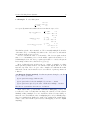
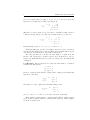
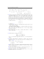

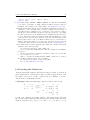

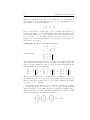

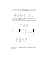
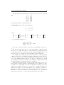

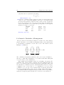


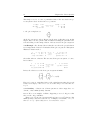


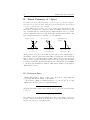
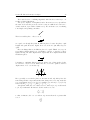

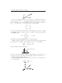
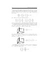

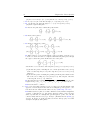
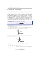

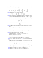
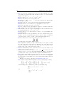


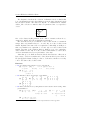

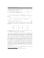
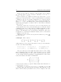

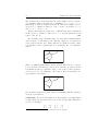


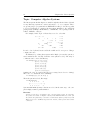


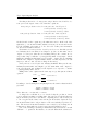


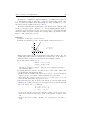
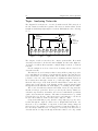

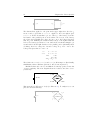
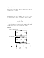

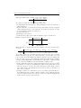
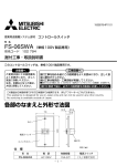

![事業報告書 [PDF/980KB/16ページ]](http://vs1.manualzilla.com/store/data/006607801_2-446596869aca3b1b9980642ca825e879-150x150.png)